TOPICAL REVIEW A review of statistical modelling and ...

IOP PUBLISHING MEASUREMENT SCIENCE AND TECHNOLOGY

Meas. Sci. Technol. 20 (2009) 052002 (22pp) doi:10.1088/0957-0233/20/5/052002

TOPICAL REVIEW

A review of statistical modelling andinference for electrical capacitancetomographyD Watzenig1 and C Fox2

1 Institute of Electrical Measurement and Measurement Signal Processing, Graz University ofTechnology, Kopernikusgasse 24, A-8010 Graz, Austria2 Department of Physics, University of Otago, PO Box 56, Dunedin, New Zealand

E-mail: [email protected] and [email protected]

Received 20 November 2007, in final form 18 December 2008Published 3 April 2009Online at stacks.iop.org/MST/20/052002

AbstractBayesian inference applied to electrical capacitance tomography, or other inverse problems,provides a framework for quantified model fitting. Estimation of unknown quantities ofinterest is based on the posterior distribution over the unknown permittivity and unobserveddata, conditioned on measured data. Key components in this framework are a prior modelrequiring a parametrization of the permittivity and a normalizable prior density, the likelihoodfunction that follows from a decomposition of measurements into deterministic and randomparts, and numerical simulation of noise-free measurements. Uncertainty in recoveredpermittivities arises from measurement noise, measurement sensitivities, model inaccuracy,discretization error and a priori uncertainty; each of these sources may be accounted for and insome cases taken advantage of. Estimates or properties of the permittivity can be calculated assummary statistics over the posterior distribution using Markov chain Monte Carlo sampling.Several modified Metropolis–Hastings algorithms are available to speed up thiscomputationally expensive step. The bias in estimates that is induced by the representation ofunknowns may be avoided by design of a prior density. The differing purpose of applicationsmeans that there is no single ‘Bayesian’ analysis. Further, differing solutions will use differentmodelling choices, perhaps influenced by the need for computational efficiency. We solve areference problem of recovering the unknown shape of a constant permittivity inclusion in anotherwise uniform background. Statistics calculated in the reference problem give accurateestimates of inclusion area, and other properties, when using measured data. The alternativesavailable for structuring inferential solutions in other applications are clarified by contrastingthem against the choice we made in our reference solution.

Keywords: statistical inversion, Bayesian inference, Markov chain Monte Carlo, electricalcapacitance tomography

1. Introduction

Electrical capacitance tomography (ECT) is an imagingmodality in which one attempts to recover the spatially varyingpermittivity of an insulating medium from measurementof capacitance outside the boundary of the medium[1, 2]. ECT is primarily used for non-invasive imaging

within inaccessible domains in applications where differingmaterials show up as contrasting permittivities. Electrodesare set in an insulating material at the outside of an insulatingtube. By applying a predefined voltage pattern to electrodesthe capacitance between pairs of electrodes can be directlyrelated to measured electric potentials, electric currents and

0957-0233/09/052002+22$30.00 1 © 2009 IOP Publishing Ltd Printed in the UK

http://dx.doi.org/10.1088/0957-0233/20/5/052002

mailto:[email protected]

mailto:[email protected]

http://stacks.iop.org/MST/20/052002

Meas. Sci. Technol. 20 (2009) 052002 Topical Review

electric charges. Measurements consist of all the capacitancesbetween pairs of electrodes, making up the matrix of trans-capacitances. The interior of the tube contains the materialwith unknown permittivity distribution that is being imaged.It is advantageous to surround the apparatus by an electricallyconducting ground shield so that measured trans-capacitancesdo not depend on the environment outside the apparatus.Measured capacitances depend on the unknown permittivity.The imaging problem is to ‘invert’ this relationship todetermine the unknown permittivity.

ECT has been proposed for a variety of target applicationssuch as imaging dilute as well as bulky multi-phase flows in oilrefinement, in the food industry and to observe pharmaceuticaland chemical processes [3–7]. Other fields of application canbe found in the characterizing of different phases in fluidizedbeds, mixing processes and combustion chambers [8–10].ECT systems can be implemented with low cost, and dueto their robustness and small failure probability are suitablefor operation under harsh environmental conditions includingthe presence of strong external electromagnetic fields [11].

The functional relationship ε(x, y) �→ C from thepermittivity distribution to the trans-capacitance matrix Cdefines the forward map. The forward map can be modelledusing the physics of the problem and is written as an ellipticpartial differential equation (PDE) of the form ∇ · (ε∇u) = q

subject to boundary conditions. The permittivity being soughtis denoted by ε and appears as the spatially varying coefficientin the PDE. The measurements made are of the boundaryvalues of the electrical potential u and flux ε ∂u

∂n.

If the electrical field u can be well approximated asa small change about a known field then the linear Bornapproximation may be used to simulate the measurementprocess (forward map). This would be the case when thepermittivity is essentially known up to a small uncertainty. Inmost applications, however, the measurement process must besimulated by solving the PDE subject to appropriate boundaryconditions. In that case the forward map is nonlinear [12, 13].

When the measurement system, consisting of the regionof interest and electrodes and the permittivity, is long in onedirection, it follows that the electric fields do not vary in thatdirection and the forward and inverse problems reduce to atwo-dimensional problem for a slice through the system. Thisis an approximation to the three-dimensional inverse problemthat is usually made to reduce computational complexity.

As a general imaging technique, ECT is necessarilylow resolution. This follows from each measurementbeing dependent on all of the permittivity, resulting inmeasurements primarily being sensitive to average, or slowlyvarying, properties. Fine-scale structure in the permittivityhas little effect on measurements. Consequently, practicalmeasurements that include noise do not unambiguously definea detailed image of the spatially varying permittivity. For thisreason it is necessary to include further information in theimaging step, such as physical constraints. In deterministicregularization methods this takes the form of a regularizingfunctional, typically a semi-norm over representations chosenon mathematical grounds. In contrast, the wider range ofrepresentations allowed by the statistical approach allows for

the inclusion of constraints or information that more closelyrepresent actual knowledge about the unknown permittivitythereby allowing genuine modelling of the unknowns to informthe imaging step. Representations and image modelling arediscussed in section 5.

The majority of ECT reconstructions reported in theliterature apply deterministic approaches such as regularizedleast squares to solve the inverse problem [14–17].Deterministic inversion consists of applying a regularapproximation to the inverse of the forward map to give asingle estimate of the unknown parameters, and includes errorsonly in terms of a single number, the ‘magnitude’ of noise.Finer details of the statistical distribution of errors are notconsidered.

The inclusion of the error process is critical for practicalsolution of inverse problems such as ECT where the forwardmap has a large range of sensitivities to features in the unknownpermittivities. Explicitly modelling the error process, andensuring that the error conforms to the model, is also aninvaluable tool in developing accurate instrumentation andan accurate forward map. All too often measurementscontain artefacts that are not part of the intended measurementmodality, or are not modelled in the forward map. Interpretingmeasurement or discretization artefacts in terms an idealizedforward map typically leads to substantial artefacts in thereconstructed permittivities [18]. We cannot over stress thevalue of the standard technique (in statistics) of examiningresiduals to validate the forward map and measurement errordistributions (see section 4).

A probabilistic model for measurement error andother uncertainties results in a probabilistic model for themeasurement process, and inversion is then a problem ofstatistical inference in which the unknown permittivity is to beestimated. The parametrization of the unknown permittivityis an important consideration as it determines the ease, ordifficulty, of stating constraints over allowable permittivities.A consequent requirement is the specification of a priordistribution over parameters since this is the primary meansof ensuring that estimates of quantities of interest are notbiased by the estimation procedure. We address the issue ofrepresentation and prior distribution in section 5. Accuratelymodelling the measurement process, including the statistics ofthe measurement error, and modelling unknowns via the priordistribution are key steps in an accurate application of Bayesianinference to inverse problems [19–21]. This approach providesa convenient setting for defining, incorporating, controllingand interpreting prior information and has a wide rangingapplicability in many inverse problems.

Statistical solutions to inverse problems have a longhistory, with notable developments in the work of Laplace andJeffreys [22] though the ingredients of a modern computationalapproach where introduced in seminal papers by Geman andGeman in 1984 [23] and Grenander and Miller in 1994[24], each for a problem in image restoration. The firstsubstantive statistical methods applied in electrical impedancetomography (EIT) were presented by Nicholls and Fox [25]and Kaipio et al [26] about 10 years ago.

By taking into account uncertainties, one can quantify therange of parameters that are consistent with measured data

2


via the posterior probability distribution. Then solutions toan ill-posed inverse problem are well-determined problems instatistical inference over that distribution. Bayesian methodsencompass much more than simply reporting a posterior modeand can be regarded as more general than regularization.

The Bayesian paradigm has many advantages overdeterministic approaches, such as robust predictive densities,posterior error estimates, direct support for optimal decisionsand the ability to treat arbitrary forward maps and errordistributions. One non-obvious advantage is the ability touse a wide range of representations of the unknown systemincluding parameter spaces that are discrete, discontinuous orof even variable dimension. Since inferential methods makeoptimal use of data, the ability to reduce data to a minimalset gives cost savings in applications where collecting data isexpensive.

The price of these advantages is presently the relativelyhigh computational cost of sampling algorithms for computingestimates. Typically, the dimension of the parameter spaceis between 50 and 105 depending on the problem to besolved. Integrations required to compute estimates such asposterior means or credible intervals are intractable throughstandard analytical or numerical quadrature techniques. Bestcurrent solutions employ Markov chain Monte Carlo (MCMC)sampling that is computationally costly. These samplingalgorithms draw samples from the posterior distribution bysimulating a Markov chain with an appropriate transitionkernel, with popular examples being the Gibbs sampler [23]and the Metropolis–Hastings (MH) algorithm [27]. Bothdiscrete and continuous problems can be treated requiring onlythe ratio of probability densities of two states to be calculated.In scenarios where material distributions change with time andreal-time performance is required, Bayesian recursive filterssuch as Kalman filters (KFs) [28, 29] and particle filters (PFs)[30] can be applied.

To overcome the computational expense of MCMCalgorithms, much current research focuses on fast alternativealgorithms in order to extend the field of applications,including non-stationary problems. We discuss these recentadvances in more detail in section 6.3.

In this article we review the current state-of-the-artin performing ECT from measured data using inferentialmethods. We have tried to also incorporate the nature of atutorial by surveying the many methods available in terms ofthe sequence of choices that need to be made to implementone solution as opposed to another.

Throughout the review we will highlight a referenceproblem in ECT, of recovering the unknown shape of asingle inclusion with unknown constant permittivity in anotherwise uniform background material, from uncertaincapacitance measurements at electrodes outside the material[31]. A schematic of this reference problem is shown infigure 1. We expect that contrasting the various choiceswe made in solving this reference application, against thealternatives available, will clarify both our solution and otherstructured inferential solutions.

The reference problem arose in an application with thegoal of quantifying void fraction (water/air) in oil pipe

electrodes

inclusion

u0

shielding

Figure 1. A schematic of the reference problem in ECT, in which asingle inclusion in permittivity is sought.

lines. Hence the area of the (two-dimensional) inclusionwas of primary interest. We therefore chose an explicitrepresentation of the boundary of the inclusion so that area issimple to calculate. That choice of representation necessarilyintroduces a bias in estimates of area (as it would withregularized inversion) and so we adjust the prior densityover inclusions to compensate (see section 5). Numericalimplementation of the forward map uses a boundary elementmethod (BEM) representation of the unknown permittivity,taking advantage of the piecewise-constant representation,coupled to a finite element method (FEM) discretization ofthe region of unchanging permittivity around the electrodes[17]. We present the posterior distribution of inclusion areaas a check on accuracy of the method. All these aspectscorrespond to choices made for this problem, some of whichwe would change given a different application or measurementmodality.

The review is organized as follows. In section 2 weintroduce the sensor technology, the requirements foran imaging system in electrical tomography, typicalmeasurements, instrumentation error, measurementuncertainties and a calibration concept. Section 3addresses data simulation for ECT. Sensor model, modellingerror as well as numerical implementation via finite andboundary elements are discussed. In section 4 we formulateECT in the Bayesian inferential framework by introducinga probabilistic model of the measurement process alongwith basic definitions for statistical inverse problems.Representation of unknowns as low-, mid- and high-leveland the issues in prior modelling are investigated insection 5. In section 6 we discuss the MCMC samplingprocedure, acceleration schemes and recent advances insampling as well as the topic of summarizing the posteriordistribution and calculation of statistics. Inversion resultsfor ECT are presented in section 7 for different permittivitydistributions using synthetic and measured data. Section 8contains a brief review on the solution of non-stationaryinverse problems. Concluding remarks are given in section 9.

3


2. Instrumentation for ECT

ECT is a non-invasive technique to examine the permittivitydistribution of closed objects by means of measurementsof coupling capacitances in a multi-electrode assembly. Ageneral setup for ECT consists of the imaging domain � ∈ R

2

or R3 containing the unknown permittivity distribution and the

domain boundary ∂� where a number of electrodes are placed.Typical configurations use 8–16 electrodes. A measurementcircuit is connected to each of the electrodes to sense theinter-electrode capacitances providing information about thepermittivity within �.

2.1. ECT sensors

Two measuring principles are typically applied to determinethe matrix of trans-capacitances, or coupling capacitances:

• Charge-based or displacement current-based method (acvoltage, low-impedance measurement) [16, 32].

• Electrode potential-based method (dc voltage, high-impedance measurement) [17].

For both methods each electrode is designated as a‘transmitting’ or as a ‘receiving’ electrode with a prescribedvoltage being applied to transmitting electrodes. In the charge-based method the receiving electrodes are held at virtual earthwith the displacement charge being measured, while in thevoltage-based approach the receiving electrodes are floatingwith the potential being measured. A comparison of the twodifferent measurement principles is given in [33].

For the charge-based method, frequencies of the typicallysinusoidal excitation signal are about 1 MHz in orderto provide sufficient sensitivity. The different hardwaredesigns of the sensing electronics, their advantages anddisadvantages have been presented by Yang [34]. Morerecently, Wegleiter et al compared the charge-based method(sinusoidal excitation signal, 40 MHz) and the potential-based method for the ECT sensor front-end in terms ofcircuit modelling, robustness to stray capacitances, hardwaredesign issues and measurement repeatability [35]. From theECT hardware design perspective, sensors need to meet thefollowing requirements and limitations:

• A selectable operation mode of each electrode(transmit/receive).

• Accurate measurement of very small inter-electrodecapacitances in the range of 1 fF to 5 pF in the presenceof stray capacitances of the order of 150 pF [34, 36].

• High dynamic range of the amplifying circuitry to covera wide range of magnitudes for electrodes adjacent andopposite to the transmitting one and to be able to considerboth low- and high-contrast problems in permittivity.

• High measurement resolution since capacitance changescaused by permittivity variations are very small.

• Shielding for all sensor circuits to reduce cross-talkbetween transmitting and receiving electrodes.

• Parallel measurement of receiving channels.• The possibility of sensor calibration (circuitry

adjustment).• A monotonic transfer function for the range of interest.

• An outer screen of the sensor head is compulsory becausethis will shield the sensor system from the ambientsystems and prevent charge disturbances on the electrodesdue to external charged objects [37].

In the charge-based method, the induced displacementcurrent is measured and converted to a voltage signal which isproportional to the inter-electrode capacitance. In comparisonto the electrode potential-based strategy, this method canbe considered a low-impedance measurement. Due tothe narrow frequency characteristics, the method is lessaffected by electromagnetic disturbances. The narrow noisebandwidth implies improved signal-to-noise ratio (SNR) andconsequently a higher resolution in measured quantities. Byincluding a tunable low-pass filter, varying stray capacitancescan be compensated in a very simple and natural way[38]. Unfortunately this approach does not work for theelectrode potential-based method [35]. A filter betweenthe electrode and the operational amplifier significantlyreduces the impedance of the input stage. Within thehigh-impedance method, the stray capacitance and the inter-electrode capacitance form a capacitive voltage divider thatreduces the amplitude of the received signal. Low-impedancemeasurements exhibit better noise characteristics and are lesssensitive to varying stray capacitances.

Due to these advantages we use a charge-based sensorbuilt at Graz University of Technology for the differentinvestigations and experiments presented in this work [35].The complete sensor font-end of the charge-based ECTsensor consists of an input resonant circuit, a low-noisecurrent-to-voltage converter, a bandpass filter, a logarithmicdemodulator and a 24 bit analog-to-digital converter controlledby a microprocessor. Figure 2 illustrates the measurementconfiguration of the ECT sensor used for permittivity imaging.The sensor has a carrier frequency of 40 MHz and comprisestwo tuneable filters adjusted by means of variable capacitancesfor stray capacitance compensation. The data acquisition hasa maximum sampling rate of 7.5 k samples/s. The receivingchannel offers linear characteristics from 10 dBμA to65 dBμA. A single measurement frame consists of 16projections, according to the 16 available transmittingelectrodes. A measurement frame consequently consists of16 × 15 = 240 entries. The first 105 displacement currentvalues of a measured frame are shown in figure 3. In mostcharge-based ECT applications the following restrictions areassumed to simplify sensor modelling:

• The permittivity is independent of the electric fieldstrength.

• The carrier frequency is constant and the wavelengthis large compared to the sensor geometry leading to anelectrostatic model.

• Stray capacitances in the longitudinal direction are notconsidered (due to length of electrodes).

The configuration used in the present study is aimedat multi-phase flow monitoring, hence a ring of electrodescovering the cross-section of a process pipe is used. The 16electrodes are evenly distributed around its boundary. Thisyields a set of 16 × 15/2 = 120 independent inter-electrodecapacitances from which the internal permittivity distributionhas to be reconstructed.

4


I/U

Logic HF

inclusion

I/U

Logic

grounded shielding

PVC tube

electrode

grounded front-end (1 of n)

grounded front-end (n of n)

μCimage reconstruction

algorithm

HF

Figure 2. Measurement configuration of the used ECT sensor. The measurement electrodes are placed around the pipe containing theimaging plane. Every electrode features dedicated transmitting and receiving hardware.

Figure 3. The first 105 values of the acquired measurement vectorfor a typical material distribution of PVC in air. The crown-shapedprofile results from the wide range of coupling capacitancesbetween the transmitting and receiving electrodes.

2.2. Sensor calibration

When using measured data special focus has to be puton the calibration of the computer model in order tosuccessfully reconstruct parameters from the data. Calibrationis performed by fitting the model to measured data for knowninternal permittivities, by adjusting stray capacitances. Straycapacitances are represented by two parameters—the radialdistance between the tube and the outer screen and thepermittivity within this space. In cases where other aspectsof the geometry are also uncertain, we include parameters todescribe the possible variation. Figure 4(a) shows the relativeerror between model and data for an empty pipe. Accordingto the normalized quantile plot in figure 4(b), the differenceis Gaussian distributed yielding a multivariate Gaussian errormodel. The remaining offset error (model to data mismatch)is corrected for the empty pipe (figure 5(a)). A second

point of calibration can be obtained by comparing simulatedand measured data for a well-defined target—a centred PVCrod in our example. The gain error between model anddata is then corrected for each electrode, figure 5(b). Notethat the prescribed calibration distribution should somehowcorrespond to an expectable permittivity distribution in termsof permittivity values and shape. It is very helpful to calibratethe model for a reference distribution that will lead to improvedSNR, which can be achieved by placing the known referenceobject in the centre of the pipe where there is low sensorsensitivity. Due to temperature fluctuations and deteriorationeffects it is recommendable to repeat the calibration in termsof offset and gain correction during operation of the sensor.

2.3. Measurement uncertainty

The sensor front-end and the subsequent instrumentationintroduce noise sources to the measurement process. Appliedvoltage also has error, but this error is not significant andwe do not consider that here (see [39] for an analysis thatdoes). To investigate the robustness and repeatability of dataacquisition, the distribution of measured displacement currentswas examined over multiple measurements with a given fixedpermittivity distribution [31]. Figure 6 shows the normalizedquantile plot and the histogram for 2000 measurements atone electrode. The measured electrode displacement currentsexhibit noise properties that can be well modelled as additivezero mean Gaussian with standard deviation σ ≈ 0.07μA.The matrix of sample correlation coefficients for all electrodesis shown in figure 7. As can be seen, off-diagonal elements areplausibly zero, so the measurement error covariance matrixis modelled as � = σ 2I where I is the identity matrix.Accordingly, the density for measuring d given permittivitydefined by θ is the multivariate Gaussian,

π(d|θ) ∝ exp

{−1

2(qm − d)T �−1(qm − d)

}, (1)

where qm denotes the vector of simulated displacementcharges.

5


0 30 60 90 120 150 180 210 240

0

1

2

3

entries in charge vector

rela

tive

err

or

betw

een m

easure

ments

and m

odel [%

]

(a)

0 1 2 3

0

1

1

1

2

2

2

3

33

1

2

3

standard normal quantiles

quantile

s o

f in

put sam

ple

QQ plot of sample data vs. standard normal

(b)

Figure 4. (a) Relative error between simulated and measured data for an empty pipe, i.e. for an air-filled pipe (εr = 1.0). (b) Normalizedquantile plot of the error between measured and simulated displacement currents. The distribution of displacement currents meets theGaussian assumption.

0 30 60 90 120 150 180 210 240

0

2

2

4

4

6

8

10

12x 10


offset err

or

[A]

(a)

0 30 60 90 120 150 180 210 2400

5

10

15


ga

in e

rro

r

(b)

Figure 5. (a) Difference between measured and simulated data for an empty pipe. This difference is referred to as offset error. (b) Gainerror between measured and simulated data corresponding to a centred PVC rod after offset correction.

3. Data simulation for ECT

3.1. Mathematical model

As discussed in section 2, measurements for ECT consist ofthe displacement charges at electrodes that result from voltagesapplied at electrodes. The forward map is the deterministicfunctional relationship from permittivity distribution to thenoise-free displacement charges. In practice it is necessaryto solve for the electric fields throughout the measurementapparatus, from which the displacement charge at electrodesmay be evaluated.

The particular set of displacement charges measured,and hence the forward map, actually depends on the set ofelectrode voltages applied during the measurement procedure.Here we describe the procedure employed in the ECT

instrumentation in Graz, where each electrode in sequence ismade ‘active’ with an asserted potential of v0 and the remainingelectrodes j �= i act as ‘receivers’ and are held at potentialvj = 0. The arrangement is surrounded by a grounded outerscreen.

We denote the measurement region by �, being theregion bounded by the electrodes and outer shield. Leti, i = 1, 2, . . . , Ne denote the boundary of electrode i whenthere are Ne electrodes, and let s be the inner boundary of theouter shield. Then the boundary to � is ∂� = ∪Ne

i=1i ∪s. Inthe absence of internal charges, the electric potential u satisfiesthe generalized Laplace equation in which the permittivityε appears as a coefficient, along with Dirichlet boundaryvalue conditions corresponding to the voltage asserted atelectrodes.

6


Figure 6. Distribution of 2000 measured displacement currents onone electrode. The distribution can be well modelled as Gaussiandistribution according to the normalized quantile plot (top) and thehistogram of the displacement currents (bottom).

1

5

9

13

16

1

5

9

1316

0

0.2

0.4

0.6

0.8

1

corr

ela

tion c

oeffic

ient

ρ xy

Figure 7. Matrix of correlation coefficients. Off-diagonal elementsare almost zero.

For the case when electrode i is held at potential v0 whileall others are held at virtual earth, then the potential ui satisfiesthe Dirichlet boundary value problem (BVP),

∇ · (ε∇ui) = 0, in �,

ui |i= v0,

ui |j= 0, j �= i,

ui |s = 0.

(2)

For brevity we have not written ε(r) and ui(r) showing thefunctional dependence on position r ∈ �, but take that spatialvariation to be implicit. The charge at the sensing electrode j

can be determined by integration of the electric displacementover the electrode boundary,

qi,j = −∮

j

ε∂ui

∂ndr, (3)

where n is the inward normal vector.It can be seen from equations (2) and (3) that the measured

displacement charges qi,j are a linear function of the voltages

asserted at electrodes ui |j. (The linear relationship is

operation by the matrix of trans-capacitances C.) Note that themeasurement set we describe, above, corresponds to assertingthe standard basis of electrode voltages to fully characterizethe linear mapping. Consequently, measurements made usingany other set of electrode voltages are a function of the set wedescribe here.

In the presence of noise, however, measurements madeusing some voltage patterns contribute more information aboutthe unknown permittivity than others. Then, for a givennumber of measurements, optimal resolution may be achievedusing an incomplete set of voltage vectors [40].

3.2. Nature of the forward map

The forward map, defined by solving the BVP (2) and thenevaluating equation (3) defines a map from Dirichlet data toNeumann data (or flux) on the boundary of the region, hencegives a representation of the ‘Dirichlet to Neumann’ (DtN)map. The measured trans-capacitance matrix C is a discreteversion of this map, between electrodes. We note, in passing,that the BVP being self-adjoint implies that C is symmetric,while the definiteness of the generalized Laplacian implies thatC is positive definite [41].

At typical SNR of 1000:1, a study of the linearizedforward map shows that ECT data contains information aboutat most 103 independent features of the permittivity [42].This number increases linearly with geometric improvementof SNR, and hence is effectively an upper bound for practicalinstrumentation. It seems plausible that a similar bound holdsfor the nonlinear problem. Hence the use of 16 electrodesin ECT, giving 120 independent electrical measurements, issufficient. Further measurements effectively only increase theSNR, which is achieved most efficiently by longer acquisitiontimes rather than more electrodes and instrumentation.

3.3. Model error

Model error occurs when (theoretical) data defined by theforward map differs from the noise-free data produced by thephysical measurement system. For many complex inverseproblems model error is the most fundamental source ofuncertainty since it is not avoidable. However, it is not usuallya significant issue in ECT where precise instrumentation isrepresented well by the electric field equations. The mostlikely source of model error is when the actual and modelledgeometries differ [43]. An interesting investigation of modelerror is given in [44], though it is important to note that inthat work the correct (simulated) model lies within the rangeof assumed models. Much more problematic is model erroroutside any known range, though frameworks for that problemhave been developed recently [45].

3.4. Computer model

While there are a few idealized problems in ECT for whichanalytic solution of the forward map is possible [46], in allpractical cases accurate simulation of data requires computerevaluation of a discretized version of equations (2) and (3).

7


Ω2, ε

2

Ω1, ε

1

Ω

∂Ω

∂Ω2

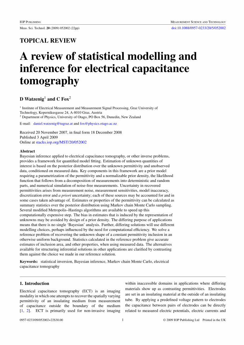
Figure 8. Cross-sectional view of an inclusion with permittivity ε2

in a background material with permittivity ε1.

Two discretization schemes are most commonly used: thefinite element method (FEM) and the boundary elementmethod (BEM). Both approaches have been applied to ECT.For the reference problem we have used a coupled FEM/BEMscheme [17, 31], with the region being imaged using a BEMformulation coupled to a FEM discretization of the insulatingpipe and region outside the electrodes.

3.4.1. Boundary element method. The BEM uses a discreteform of the boundary integral equations [47] that express fieldswithin regions of constant permittivity in terms of values atthe boundary of the region. Hence BEM is applicable toproblems where the permittivity is piecewise constant, as inour reference problem, and has been used extensively in ECT[30, 48, 49].

Figure 8 illustrates a BEM discretization of an ellipticinclusion (ε2) in an otherwise constant background materialwith permittivity ε1. For simplicity, linear boundary elementsare used in the reference problem, and the electric potentialand its normal derivative are assumed to be constant on eachof the Nb elements, though higher order schemes are possible[50]. The resulting system to be solved has the form(

K + 12I

)u = Hq, (4)

where u is a known vector of Dirichlet values, q is the vectorof Neumann values being solved for, and the matrices K andH are dense, not symmetric, and of size Nb × Nb when thereare Nb boundary elements in total.

BEM suffers from many potential numerical difficultiesthat make it problematic for use in solving inverse problemsby iterative methods, whether statistical or deterministic. Onesuch problem is that the matrix system to be solved becomeshighly ill-conditioned when regions are thin or significantlynon-convex. While these geometry-based problems have well-known solutions, they do add to the complexity of computercodes; otherwise they pose a genuine difficulty for samplingalgorithms since the state is required to explore all possiblestates including those for which BEM fails. A ‘fix’ that wehave implemented for the reference problem is to modifythe prior over boundaries to exclude states that present anumerical difficulty, such as polygonal boundaries with thin‘spikes’. This pragmatic solution is unlikely to affect results

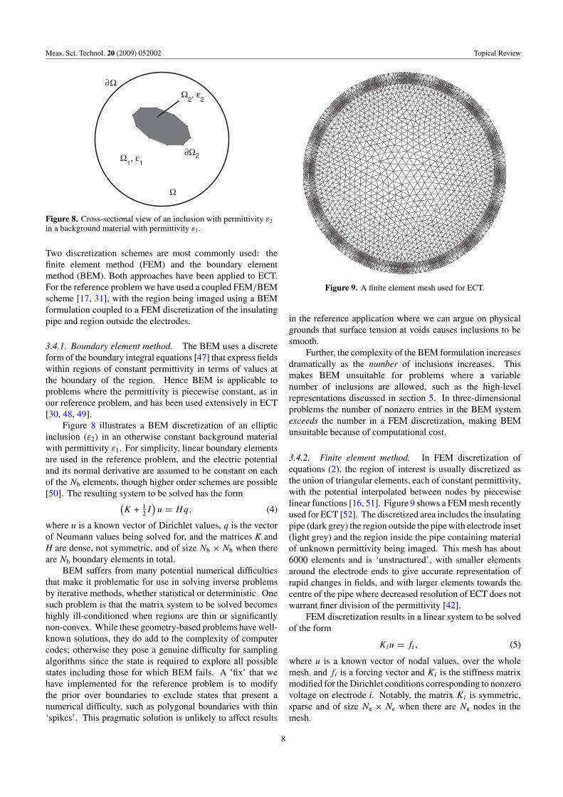
Figure 9. A finite element mesh used for ECT.

in the reference application where we can argue on physicalgrounds that surface tension at voids causes inclusions to besmooth.

Further, the complexity of the BEM formulation increasesdramatically as the number of inclusions increases. Thismakes BEM unsuitable for problems where a variablenumber of inclusions are allowed, such as the high-levelrepresentations discussed in section 5. In three-dimensionalproblems the number of nonzero entries in the BEM systemexceeds the number in a FEM discretization, making BEMunsuitable because of computational cost.

3.4.2. Finite element method. In FEM discretization ofequations (2), the region of interest is usually discretized asthe union of triangular elements, each of constant permittivity,with the potential interpolated between nodes by piecewiselinear functions [16, 51]. Figure 9 shows a FEM mesh recentlyused for ECT [52]. The discretized area includes the insulatingpipe (dark grey) the region outside the pipe with electrode inset(light grey) and the region inside the pipe containing materialof unknown permittivity being imaged. This mesh has about6000 elements and is ‘unstructured’, with smaller elementsaround the electrode ends to give accurate representation ofrapid changes in fields, and with larger elements towards thecentre of the pipe where decreased resolution of ECT does notwarrant finer division of the permittivity [42].

FEM discretization results in a linear system to be solvedof the form

Kiu = fi, (5)

where u is a known vector of nodal values, over the wholemesh, and fi is a forcing vector and Ki is the stiffness matrixmodified for the Dirichlet conditions corresponding to nonzerovoltage on electrode i. Notably, the matrix Ki is symmetric,sparse and of size Ne × Ne when there are Ne nodes in themesh.

8


Data is simulated by solving the FEM equation (5) formultiple fi , one for each asserted voltage pattern. For two-dimensional problems, efficient solution is achieved by firstoperating by a bandwidth reducing permutation followedby Cholesky factoring of Ki [52]. For three-dimensionalproblems with fine meshes, multigrid solvers are significantlyfaster, and also provide access to cheap solutions at coarsescales that may be utilized within the MCMC to decreaseoverall compute time [53].

For the efficient numerical implementation of (3) theelectrode charge is directly calculated from the node potentialsui for sending electrode i and the global finite element stiffnessmatrix free of boundary conditions K without having to resortto gradient calculations,

qi,j =∑nj

kTnj

ui . (6)

The sum contains the scalar products of the rows of the stiffnessmatrix corresponding to the nodes nj of the sensing electrodesand the solution vector.

In our recent work in ECT, and EIT, we have used theFEM discretization only, for reasons of speed, generality andfor the generic structure of the FEM system of equations thatallows very efficient calculation Jacobians and local updates[39, 54]. The permittivity ε(r) defined by parameters θ is firstmapped to FEM elements, and the solution is then calculated.

3.4.3. Discretization error. In BEM or FEM formulations,the number of elements used is a compromise betweennumerical accuracy and computational effort. However,good imaging results require that the discretization be madesufficiently fine so that errors introduced through discretizationare smaller than measurements errors. The mesh depictedin figure 9 was designed as the coarsest mesh meeting thisrequirement. Failing to achieve that, and not includingdiscretization errors correctly, leads to substantially increasederrors in the recovered permittivity. This important resultis demonstrated explicitly in [18, 55]. Coarse numericaldiscretization has been used, either in conjunction withaccurate solvers or by including discretization error, to speedup sample-based inference in ECT. Schemes for achieving thisare covered in section 6.3.2.

3.4.4. Factorizations and derivatives. When efficientsolution of systems (4) and (5) is performed by first factorizingmatrices, it is feasible to directly maintain the QR factorizationin BEM, and the Cholesky factorization in FEM [56],for potential gain in computational efficiency. Both theseschemes have been applied to EIT, as has direct updating ofsolutions using the Woodbury formula [39] though the latteris numerically unstable in the long term. Both FEM and BEMformulations also allow efficient calculation of derivatives.In a FEM formulation, operation by the Jacobian from finiteelement coefficients to solutions may be performed using onlysolutions at the current state [13], with gradients with respectto the parameter vector calculated using the chain rule. InBEM formulations, expressions for the Frechet derivative ofthe forward map allow evaluation of the gradient with respect

to the boundary by solving a non-homogeneous equation withthe current BEM matrices [57].

4. Formulation of ECT as Bayesian inference

Application of Bayesian inference to ECT provides aframework for quantified model fitting, by explicitly formingthe conditional distribution of parameters defining thepermittivity and unobserved data, given observed data. Thedistribution over parameters quantifies the degree to whichmeasurements combined with other knowledge determinethe unknown permittivity, or properties of the permittivity.The uncertainty over permittivities arises from several mainsources: measurement noise, measurement sensitivitiesthat are small compared to the noise, model inaccuracy,discretization error and a priori uncertainty in the trueparameters.

Defining a distribution over allowable permittivitiesincludes the formulation used in deterministic approachesof seeking a single solution, when the distribution is highlypeaked around a single parameter value. It also allows for moregeneral circumstances of multi-modal densities correspondingto multiple solutions being consistent with the data. However,the real power for high-dimensional inverse problems is thatrobust estimates may be calculated over the density, whereasmodes of the density corresponding to deterministic solutionscan give results that are highly sensitive to the particularrealization of noise in the measured data [12, 58].

4.1. Likelihood function

The unavoidable presence of measurement noise means thatthe measurement process is probabilistic, as we saw insection 2.3. The inverse problem is then naturally a problem ofstatistical inference. In the following we outline the inferentialformulation in a general setting and relate it to the referenceproblem in ECT.

For the sake of definiteness, consider the case of additivenoise n with probability density function πn(n). In most casesthe measurement noise has a multivariate Gaussian or a Gibbsdistribution [55], though it is important to note that any noiseprocess may be treated. Then the measurement process can bewritten as

d = A(θ) + n, (7)

where A(θ) denotes the forward map describing the mappingfrom permittivity defined by θ to noise-free measurements,and n is a realization from the noise process.

Equation (7) represents a decomposition of measurementsinto deterministic (A(θ)) and random parts (n). For theinstrumentation described in section 2 the decomposition wasrelatively clear, largely because of careful construction ofinstrumentation and repeated improvement to remove strayeffects. In general, however, the decomposition is somewhatarbitrary since it is possible to describe any effect as random.The random part has a minimal component consisting ofthermal and shot noise in the electronics, and digitizationerrors, and often includes external interference, though the

9


latter can be modelled as deterministic through the use of‘nuisance variables’. Our experience is that quality of imaging,and inference, is always improved by putting as much aspossible into the deterministic part, though complexity ofphysical modelling and computation often set a practical limit.

The conditional probability density for measuring d giventhat θ is the true parameter then follows from equation (7), andis

π(d|θ) = πn (d − A(θ)) (8)

since the change of variables has determinant 1. Making aset of measurements corresponds to drawing a sample d fromπ(d|θ) which is a probability distribution parametrized by theunknowns θ via the forward map A.

As a function of θ, π(d|θ) is not a probability densityfunction and is usually written l(θ |d) and referred to as thelikelihood function. The likelihood principle is the formalstatement that all information that data d contains about theunknown parameters θ is encoded in the likelihood function,for fixed d.

The form of the likelihood function we use in thereference problem is given in equation (1), accounting forerrors in measured displacement charges. In practice thevoltages asserted at electrodes are also imprecisely knownand the nominal values should be considered as part of themeasurement set. A framework for that more completeanalysis is given in [39], which augments rather than changesour development here.

4.2. Bayesian inference

Statistical inference aims at recovering parameters θ andassessing the uncertainty about these parameters based onall available knowledge of the measurement process and themeasurement noise as well as information about the unknownsprior to the measurement. In the Bayesian formulation,inference about θ is based on the posterior density π(θ |d)

π(θ |d) = l(θ |d)π(θ)

π(d), (9)

where π(θ) denotes the prior density, expressing theinformation of θ prior to the measurement of d. The topicof prior distributions is covered in section 5. The posteriordensity π(θ |d) denotes the probability density over θ giventhe prior information and the measurements. The denominatorπ(d) = ∫

θl(θ |d)π(θ)dθ is a finite normalizing constant since

the sum of the posterior probability density function over allpossible causes must be equal to one. In case of a fixedforward map such as in ECT this probability density does notneed to be calculated explicitly and we can work with the non-normalized posterior distribution determined by the likelihoodfunction and the prior density function.

In this inferential framework, solution to the inverseproblem corresponds to providing statistics that summarizethe posterior distribution. How to summarize the posteriordepends greatly on the application under consideration. Forexample a posterior distribution peaked around a single valueis well summarized by giving just that value, and a measureof width, corresponding to a well-defined inverse image with

uncertainty bounds. Bimodal distributions need at least twovalues reported, and so on. Summary statistics of somefunction f (θ) may be calculated as expectations over theposterior

E[f (·)] =∫

f (θ)π(θ |d) dθ (10)

with common statistics being the mean E[θ ] and thevariance E[(θ − E[θ ])2] of θ . Since parameter space is usually of high dimension, the integrals requiredcannot be performed analytically, or using deterministicnumerical methods such as Gaussian quadrature. Fortunately,Monte Carlo approximations can be evaluated with tractablecomputation, as discussed in section 6.

4.3. Sensor calibration

Our inferential formulation for the reference problem isactually a little more complicated than the general proceduregiven above, because of the sensor calibration step. Thepermittivity ε is decomposed (in this section only) intounknown and fixed parts, with separate domains. We writeεext = ε|�ext , εint = ε|�int where �int is the interior of thepipe, that in the application contains material of unknownpermittivity, and �ext is the pipe and exterior region in whichthe electrodes are fixed.

Calibration consists of estimating the exterior permittivityεext parametrized by θext containing a few permittivity valuesas well as a few parameters describing possible deviationsfrom ideal geometry. Repeated measurements are made withsimple known interior permittivities parametrized by (known)parameter θint, allowing the simple best-fit estimate

θext = arg maxθext

π(d|θext, θint). (11)

We then fix, i.e. condition on, this estimate to give thelikelihood function for inference about unknown θint.

4.4. A short reading list in Bayesian inference

Our treatment here of the Bayesian formulation is necessarilycursory, and light on technical details. For more details ofBayesian formulations of inferential problems in general (notnecessarily for inverse problems or ECT) we recommend[59]. Computing expectations over complex densities inparameter space necessarily use sampling algorithms. Apractical introduction is given in the first few chapters of[60]. More technical results regarding convergence of MCMCmethods can be found in [61]. A kit-bag of useful ideas forspeeding up MCMC can be found in [62].

5. Representation of unknowns and the priordistribution

Since the primary unknown, i.e. the permittivity, is a spatiallyvarying function, recent developments in spatial statistics [63]and pattern theory [64] are directly applicable. They providemeans of stating loose, generic and specific information aboutthe unknown permittivity, as befits the application. A goodoverview of image analysis from the statisticians viewpoint

10


is [19]. The central components of all image models are therepresentation of the unknown image, i.e. the parameters orcoordinates used to define an image, and a normalizable priordensity over the space of representations.

Representation and knowledge are inextricably linked,and so the reason for choosing a particular representationshould be largely determined by the type of knowledge onewants to express or calculate. For example, in the referenceECT problem we know that the permittivity is two valued(background and inclusion) and our primary interest is thearea of the inclusion. A polygonal representation of theinclusion, with background and inclusion permittivity values,is a suitable representation since it automatically states thephysical knowledge and allows straightforward calculation ofthe area. In contrast, a grey-scale pixel image would requirefurther constraints to state the prior knowledge, while thecalculation of inclusion area is a non-trivial task requiringidentification of the inclusion boundary amongst other steps.In many applications, the use of representations that providequick access to properties of interest can provide substantialefficiencies, since then image restoration and image analysisare not separate tasks.

It is useful to classify representations, and priors, as low-level, mid-level and high-level. Low-level representationsare local and generic, and usually very high-dimensional,such as grey-scale pixel images, or the vector of elementcoefficients in a FEM discretization. These representationscan be used for any image, but are inconvenient for stating orcalculating anything other than local structural information.Mid-level models are also generic, but provide convenientways of expressing quantities of interest such as geometricfeatures of objects, or between objects. An example is thepolygonal representation used in the reference problem. High-level models capture important, possibly complex, features ofthe images and are useful for answering global questions aboutthe image, such as counting the number of objects of a giventype.

The formulation of a statistically sensible priordistribution over the space of representations is a majorpractical difference between regularization and Bayesianinferential methods. Consistency of the statistical formulationand guaranteed convergence of sampling algorithms bothrequire that the prior density be normalizable. We find thatthe requirement of specifying a parameter space with finitevolume has the added benefit of forcing us to be explicit whenmodelling the image. In the Bayesian framework it is typical totest modelling assumptions by drawing several samples fromthe prior distribution and ensuring that they look reasonable.In contrast, typical regularization functionals would fail theserequirements.

The role of the prior distribution is typically different forlow- mid- and high-level representations, as we will see in thefollowing review of representations and priors for ECT.

5.1. Low-level models

Low-level representations use grey-scale values over a pixel(voxel) lattice, or a fixed FEM discretization, and can be used

for arbitrary permittivity distributions. Grey values may berestricted to two values (black/white) [13, 53, 65] or a finite setof allowable values [25] or more typically to any positive value[26, 44]. Low-level prior distributions usually have the rolefamiliar in regularization of preferring smoothness, sometimesmodified to implicitly allow non-smooth behaviour such asedge processes. Good overviews of low-level prior modellingin EIT are given by Kaipio et al [26, 55] and Siltanen et al[66], and for single-photon emission computed tomographyby Aykroyd et al [67].

The following gives a brief discussion of low-level priormodels used for ECT:

• Gaussian priors. The Gaussian white noise prior, inequation (12), is the most widely used prior model,since the diagonal covariance matrix generalizes standardTikhonov regularization

π(θ) ∝ exp

{− 1

2σ 2‖θ − θ‖2

}. (12)

The variance σ 2 describes the variability of the unknownparameters θ around the assumed mean value θ .

• Markov random field (MRF) priors. Smoothness priorsare special cases of MRFs in which the conditionaldensity over pixels (elements) depends on the remainingparameters only through its neighbours. A typical MRFprior is the total variation prior [55] given by

T V (θ) =M∑i=1

∑j∈Ni

lij |θi − θj |, (13)

where Ni ⊂ {1, 2, . . . , M} is a set of possible neighboursof θi with i /∈ Ni and i, j are neighbours with a commonedge of length lij . Common neighbourhood structuresare induced by the pixel lattice or FEM mesh. The priorprobability density is then π(θ) ∝ exp{−βT V (θ)}, whereβ is a smoothing parameter. We note that π(θ) is a Gibbsdistribution [23]. An application of a non-standard MRFprior can be found in the recovering of resistor values in anelectrical network from electrical measurements collectedat the boundary [13].

• Impulse noise priors. Such priors are typically applied tolow contrast problems where small regions in an otherwiseuniform background have to be recovered (e.g. bright starsin black sky). Representative priors are the maximumentropy prior [68] and the L1 prior [69].

• Sample-based priors. In some applications it is possible todefine a representative ensemble of images that may occur,through a set of sample images that define an empiricalprior density. This prior has been used in the context ofpixel image models [55].

5.2. Mid-level models

Mid-level representations allow access to generic structuralinformation about the unknown permittivity, without imposingcomplex structure. Examples of mid-level priors used for

11


ECT, or EIT, include the ‘type field’ or segmented MRFprior [25, 70, 71], coloured continuum triangulations [72] andexplicit boundaries between piecewise-constant permittivitiessuch as the polygonal boundary used in the referenceapplication (though some classify the latter as high level [19]).

Representing unknowns as piecewise constant viaboundaries has been widespread in ECT, with generalcontour models based on Fourier descriptors [66, 73], splines[74], radial basis functions [54], front points [75], Beziercurves [76] and simple polygons [48, 49, 54]. Few-parameter representations of smooth contours [77, 78] andsmooth transitions [42] between regions of different physicalproperties have also been used.

Our solution to the reference problem uses a polygonalrepresentation of the boundary, so the permittivity is definedby the parameter θ = ((x1, y1), (x2, y2), . . . , (xn, yn)) givingthe vertexes of an n-gon for some fixed n typically in therange 8–32. We also include the two permittivity values,but we will omit that consideration here for clarity. A basicprior density over this representation is to sample each vertex(xk, yk) uniformly in area from the allowable domain � andrestrict to simple polygons, i.e. not self crossing. This priordensity has the form

π(θ) ∝ I (θ), (14)

where I is the indicator function for θ representing a feasiblepolygon. That is, the prior density is constant over allowablepolygons. The change of variables relation for probabilitydistributions shows that a uniform density in vertex positiongives a density over area that scales as (area)−1/2. Hencefor large polygons, and inclusions, where most polygons aresimple, this prior puts greater weight on small areas resultingin estimated areas that will always be smaller than the truearea. The constraint that the polygon be simple complicatesthis picture for small area inclusions, since a greater proportionof small polygons are self-crossing. An empirical distributionover prior area, given by sampling from the prior, is shownin figure 10 for n = 8. The overall effect is that the area oflarge inclusions will be underestimated while the area of smallinclusions will be overestimated, with the division between‘small’ and ‘large’ depending on the number of vertexes n.This effect necessarily occurs in regularized or least-squaresfitting of contour-based models, since effectively the constantprior model is used.

Since we are primarily interested in area of inclusions, weremove this bias by explicitly specifying a prior in terms ofarea, given in equation (15) [79], though scaling based on theempirical distribution to give a prior that is non-informativewith respect to area is also possible [52]. The circumferenceof the inclusion c(θ) with respect to the circumference of acircle with an area equal to the area of the polygon (θ) iscalculated. The variance σ 2

pr is chosen to be small to penalizesmall and large areas

π(θ) ∝ exp

{− 1

2σ 2pr

(c(θ)

2√

(θ)π− 1

)}I (θ) . (15)

Redundancy in the polygonal representation can also leadto numerical inefficiency without contributing to quality of

0 0.5 1 1.5 2 2.5 3 3.5 40

1

2

3

4

5

6

7

8

9

10x 10

4

area (arbitrary units)

num

ber

of s

ampl

es

Figure 10. Empirical distribution over area for indicator functionprior density.

reconstructions. These difficulties can be circumvented byfurther modifying the prior distribution.

We briefly mention some other mid-level priors that havebeen used in ECT.

• Smoothness prior over star-shaped polygons. Aykroydet al represented polygons in a star-shaped manner,parametrizing the centre of the star and radii r =(r1, r2, . . . , rn) at m equi-spaced angles [48]. Theyspecified a prior intended to give smoothness of theboundary, using

π(r) ∝ exp

⎧⎨⎩− 1

2ν2

∑i∼j

(ri − rj )2

⎫⎬⎭ , (16)

where i ∼ j indicates neighbouring radii. In the contextof the reference problem, it is interesting to note that thisprior will exhibit the bias in (large) area outlined above,as is evident from computed results.

• Structural priors. Especially in medical imaging,geometry and position of structures are often knowna priori. Hence, it is reasonable to include this knowledgein the form of a prior model [80, 81], or equivalently byfusing different sensing modalities. An example is theuse of ultrasound tomography to recover boundaries foruse in ECT [82].

Parameter spaces for mid-level models are not-usuallylinear spaces. Consequently, non-uniqueness or ill-posednessresults for forward maps based on the theory of linear spacesdo not apply. We have experience of industrial applicationswhere an inverse problem that was under-determined for alow-level linear-space model became over-determined for amid-level model and required reduction of the measurementset to avoid excessive computation.

5.3. High-level models

High-level models incorporate structural information bymodelling objects in the image. Representations are typically

12


variable dimension allowing for differing numbers of objects.Hence, perhaps contrary to expectation, high-level modelsare usually higher (infinite) dimensional models than low-or mid-level models. High-level prior densities are definedover individual objects and, importantly, also over the numberof objects to provide a trade off between model complexityand data fit, as in an ‘information criterion’. A high-levelrepresentation was used in [70] allowing conditioning on, andcounting of ‘blobs’ in an EIT application. It seems inevitablethat high-level deformable template models [64] developed formedical imaging, and other applications, will find applicationin ECT.

6. Summarizing the posterior distribution

In the following we write the abbreviated π(θ) for the posteriordensity π(θ |d). Exploration of the posterior distributionis performed using Markov chain Monte Carlo (MCMC)sampling that generates a Markov chain with equilibriumdistribution π by simulating an appropriate transition kernel[83, 84].

The long-term output of MCMC samplers are states θi

distributed according to π , and we write θi ∼ π . The empiricaldistribution defined this way can be used to summarize π , or inexploratory analyses the samples may simply be displayed togain understanding about the nature of permittivities consistentwith the data. In many applications a single sample fromπ provides a better reconstruction than regularized inversion[58]. A few independent samples, say 2–4, can establish ascale and nature of ambiguity in the allowable permittivities(see e.g. [20]), while extensive sampling allows quantitativeestimates of posterior variability in applications where thatis needed. Computed results for the reference problem,presented in section 7, are designed to present the range ofstates in the posterior by summarizing posterior area andboundary processes.

6.1. Metropolis–Hastings algorithm

The Metropolis–Hastings (MH) algorithm generates a Markovchain with equilibrium distribution π by simulating a suitabletransition kernel [27].

It uses a proposal density q(θ, θ ′) to suggest a new stateθ ′ when at state θ , i.e. a possible move θ → θ ′. The proposalis accepted or rejected according to a rule that ensures thedesired ergodic behaviour. Choice of the proposal densityis largely arbitrary, with convergence guaranteed when theresulting MCMC is irreducible and aperiodic. However, thechoice of proposal distribution critically affects efficiency ofthe resulting sampler, with design of a good proposal beingsomething of an art.

The standard MH formalism has been extended to dealwith transitions in state space with differing dimension [83],allowing insertion and deletion of parameters [72, 85, 86].Even though we do not use variable-dimension states inthe reference example we prefer this ‘reversible jump’, orMetropolis–Hastings–Green (MHG), formalism as it greatlysimplifies calculation of acceptance probabilities for thesubspace moves that we employ.

The reversible jump formalism considers the compositeparameter (θ, γ ) where θ is the usual state vector, and γ is thevector of random numbers used to compute the proposal θ ′.Similarly, (θ ′, γ ′) is the composite parameter for the reverseproposal. Then the MCMC sampling algorithm with MHdynamics can be written as

Let the chain be in state θn = θ , then θn+1 is determined in thefollowing way:

• Propose a new candidate state θ ′ from θ with someproposal density q(θ, θ ′).

• Calculate the MH acceptance ratio

α(θ, θ ′) = min

(1,

π(θ ′|d)q(γ ′)π(θ |d)q(γ )

∣∣∣∣∂(θ ′, γ ′)∂(θ, γ )

∣∣∣∣) . (17)

• Set θn+1 = θ ′ with probability α(θ, θ ′) , i.e. accept theproposed state, otherwise set θn+1 = θ , i.e. reject.

• Repeat

The last factor in equation (17) denotes the Jacobiandeterminant of the transformation from (θ, γ ) to (θ ′, γ ′).

6.2. Monte Carlo integration

Quantitative estimates from the posterior distribution requirecomputing the expectations in equation (10). Given samples{θi}i=1,2,...,N from π , the required integral may be computedusing the Monte Carlo approximation∫

f (θ)π(θ) dθ ≈ 1

N

N∑i=1

f (θi). (18)

According to the law of large numbers, equation (18) holdsto any desired accuracy for sufficiently large N. In addition, itfollows from the central limit theorem that the approximationerror is independent of dimensionality of the state spaceand hence MCMC methods are suitable for high-dimensionalproblems. The variance of the approximation error is givenby

Var

(1

N

N∑i=1

f (θi) −∫

f (θ)π(θ) dθ

)

≈ Var(f )

N

⎛⎝1 + 2N∑

j=1

(1 − j

N

)ρj

⎞⎠︸︷︷︸

τf

(19)

with Var(f ) = E[f (θ)2 −μ2

f

]. The factor ρj = Cj /C0 is the

normalized autocovariance function (ACF) and Cj is the ACFat lag j , i.e. Cj is the covariance between the values taken by f

for two random states of the chain θi and θi+j . Consequently,the less correlated are consecutive states of the chain the moreaccurate are estimates. When {θi}Ni=1 are independent, i.e.uncorrelated, samples and the estimator for the mean of f isfN = 1

N

∑Ni=1 f (θi) and the variance of the estimator is

Var(f N) = Var(f )

N. (20)

However, almost always {θi}Ni=1 produced by MCMC is asequence of correlated samples. The rate τf /N at which the

13


variance Var(f N ) reduces in equation (19) is called statisticalefficiency, and we write the variance reduction for independentsamples as

Var(f N ) = τf

Var(f )

N. (21)

The quantity τf is called the integrated autocorrelation time(IACT) and can be interpreted as the number of correlatedsamples with the same variance-reducing power as oneindependent sample. For a given posterior distribution theMarkov chain should be designed in a way that τf is as small aspossible so that small variance σfN

= Var(f N ) of the estimatef N is achieved with minimal sample size N.

6.3. Acceleration schemes for Metropolis–Hastings MCMC

A major drawback of MCMC sampling is its computationalexpense since the forward problem has to be solved hundredsof thousands times to explore the posterior distribution. Hencemuch research effort has gone into finding ways of acceleratingthe basic MH algorithm. We review several such schemes,dwelling on those that have found application in impedancetomography.

6.3.1. Simulated tempering. Consider the case where theMH algorithm is used to sample from posterior distributionπ(·) using proposal distribution q(θ, θ ′) and it is found thatthe resulting chain is evolving slowly, or worse still is gettingstuck. This can happen because of multi-modality of π(·), orbecause of strong correlations as is typical in inverse problemswhere the support of π(·) can be effectively a low-dimensionalsubspace of . Simulated tempering (with the name andidea adapted from simulated annealing for optimization) is ageneral method that can overcome some of these difficulties,while using the existing proposal distribution.

The methods augments the state space to ×{0, 1, . . . , N} and defines a set of distributions {πk(·)}Nk=0where π0 = π and π1(·), π2(·), . . . , πN(·) are a sequence ofdistributions that are increasingly easy to sample from. Thedistribution over the augmented space is taken as

π(x, k) = λkπk(x), (22)

where λ0, λ1, . . . , λN are pseudo prior constants with∑Nk=1 λk = 1. Transitions for a fixed k are derived from

the proposal q(θ, θ ′) and are interspersed with proposalsthat change k (perhaps by a random walk in k) withboth accepted/rejected by a standard Metropolis–Hastingsalgorithm. The random walk then occurs in (θ, k) space.Samples that have k = 0, i.e. from the conditional densityπ(θ, k|k = 0), are samples from the desired distribution.

A simple example of such a sequence is the schemedue to Marinari and Parisi [87] who introduced simulatedtempering. Define the positive numbers (inverse temperatures)1 = β0 < β1 < · · · < βN . The sequence of distributionsis then given by πk(θ) = λkπ

βk (θ) which are increasinglyunimodal. The opposite regime, of increasing temperature, hasfound greater success in impedance tomography applicationswhere high-accuracy data leads to posterior distributions thatare too narrow to easily sample [70].

Parallel tempering is similar to simulated temperingexcept that the N chains (one for each value of k) are maintainedsimultaneously. An example is the Metropolis coupledMCMC in [84] that simultaneously runs chains with the spatialparameters increasingly coarsened, defining a sequence ofdistributions as above.

6.3.2. Using approximations to the forward map. As a meansof model reduction (and counteracting inverse crimes) Kaipioand Somersalo [55] introduced the ‘enhanced error model’ tocorrect for discretization errors introduced by coarse numericalapproximations. For the case of Gaussian prior and noisedistributions, they considered the accurate model d = Aθ + n

and the coarse approximation d = Aθ + n where θ = Pθ isa coarse approximation to the unknowns x resulting from aprojection by P, and A is the (cheap) approximation to A oncoarse variables. Then

n = (A − AP )θ + n (23)

defines the enhanced error model by assuming that the twoterms on the right-hand side are uncorrelated. Use of thecoarse approximation necessarily increases the uncertaintyof recovered values, since discretization error has beenintroduced. However, Kaipio and Somersalo [55] giveexamples in which a tolerably small increase in posterioruncertainty is traded for a huge reduction in compute timewithout introducing bias in estimates, and demonstrate thataccurate real-time inversion is possible.

A second use of approximations was introduced byChristen and Fox [13] who considered the state-dependentapproximation π∗

θ (·) to the posterior distribution calculatedusing a cheap approximation to the forward map, to give amodified Metropolis–Hastings MCMC. Once a proposal isgenerated from the proposal distribution q(θ, θ ′), to avoidcalculating π(θ ′) for proposals that are rejected, they firstevaluate the proposal using the approximation π∗

θ (θ ′) to createa second proposal distribution q∗(θ, θ ′) that is then used in astandard Metropolis–Hastings algorithm.

Christen and Fox [13] present an example using a locallinearization, and demonstrate an order of magnitude speedupfor a problem in electrical impedance imaging. Lee useda coarse BEM approximation to speed up inverse obstaclescattering [57], while coarsened solutions available in a multi-level (multigrid) solver were used for a problem equivalent toECT in [53].

6.4. Summary statistics

The posterior distribution is typically defined over a high-dimensional parameter space so direct visualization is notpossible. However, in the Bayesian framework we areable to calculate summary statistics that quantify andexamine the feasible solutions to the inverse problem.Histograms for properties, posterior variability of parameters,and expectations can be easily derived from the posteriordistribution. Scatter plots allow for an illustrative andmeaningful depiction of the range of feasible solutions (seesection 7).

14


More generic summary statistics of a posterior distributionare the point estimates (or modes) and interval estimates,computed via numerical optimization. The most commonpoint estimate is the maximum a posteriori (MAP) estimatorgiven by

θMAP = arg maxθ

π(θ |d) (24)

since this mode of the posterior distribution generalizesregularized inversion. For example, when the noise isadditive zero mean Gaussian with variance σ 2, and weuse a simple Gaussian prior π(θ), then the MAP estimatebecomes the classical deterministic setting known as Tikhonovregularization [12]. In case of multi-modal posteriordistributions, or if the mode of the posterior distributionlies far away from the bulk of the posterior distribution, theMAP estimate provides an unsatisfactory summary of feasibleparameter values, and can be very unrepresentative of thesupport of the posterior distribution.

The estimate given by the mode of the likelihood function,often erroneously described as the estimate that correspondsto the set of parameters which are most likely to generatethe measured data, is called the maximum likelihood (ML)estimate and is defined by

θML = arg maxθ

l(θ |d). (25)

This estimator is equivalent to solving the inverse problemwithout taking regularization into account [55]. Hence, inill-posed inverse problems such as ECT the ML estimate isseldom useful.

A more robust point estimate is the conditional mean (CM)of the parameters conditioned on the measured data d,

θCM = E[θ |d] =∫

θπ(θ |d) dθ. (26)

A common interval estimate is the conditional covariance (CC)estimate given by

Cov(θ |d) =∫

(θ − θCM)(θ − θCM)Tπ(θ |d) dθ ∈ Rn×n.

(27)

The price of robustness in the CM and CC estimates isan integration over the high-dimensional parameter space,requiring extensive MCMC sampling.

7. Numerical examples

The previous sections give a complete formulation of ECTin the Bayesian inferential framework. The uncertainties inmeasured data, i.e. in measured inter-electrode capacitances,and the range of feasible images are taken into account bystatistically modelling the measurement process according tosection 4.

Our representation of the true parameters is the setof points {(xi, yi)}, giving vertexes defining a polygonalboundary of a material inclusion [31, 48, 88, 89]. Thisset denoted θ ∈ defines a ‘state’ in our reconstructionalgorithm. The forward map in section 3 relates the state θ tonoise-free measurements. The omnipresence of measurement

noise implies that in practice a range of data may be measuredfor a given state θ . Let π(d|θ) denote the probability densityfunction over allowable measurements d for a given true stateθ . Making a set of measurements corresponds to drawing asample d from π(d|θ).

Our objective now is to work out what we can sayabout the parameter θ given measurements d. Inferenceabout θ is based on the posterior density π(θ |d) applyingBayes’ theorem (9). The posterior density π(θ |d) givesthe probability density over allowable states θ conditionedon measurements and prior information. Summarizing theposterior distribution corresponds to solving the inverseproblem since that gives knowledge of the allowable valuesof parameters with uncertainties, etc.

In section 2.3 we have derived the likelihood functionl(θ |d) as a function of θ for the given ECT system. Note thatl(θ |d) is generally not a probability function.

Since in our ECT application the estimation of the processparameter material or void fraction is of primary interest, wehave to specify an appropriate prior π(θ) that allows for anunbiased reconstruction of inclusion area. To avoid this biaswe specify a prior density in terms of area directly, givenin equation (15) in section 5 [79]. The circumference of theinclusion c(θ) with respect to the circumference of a circle withan area equal to the area of the polygon (θ) is calculated. Thevariance σ 2

pr is chosen to be small to penalize small and largeareas.

Based on the accurately modelled forward map, thespecified prior distribution π(θ) for the shape and permittivityof the material inclusion, and the measurement noise model,we are able to give a posterior distribution π(θ |d) for inclusionconditioned on measured data

π(θ |d) ∝ π(θ)l(θ |d) = exp

{− 1

2σ 2pr

(c(θ)

2√

π(θ)− 1

)

−1

2(qm − d)T �−1(qm − d)

}. (28)

It is this distribution we explore to learn about the unknownpermittivity, by applying MCMC sampling with Metropolis–Hastings dynamics.

We use several types of update to propose a new stateθ ′, usually referred to as ‘moves’ [79]. The choice andthe combination of such moves is a crucial issue in MCMCsampling in order to ensure ergodic behaviour of the chainwithin useful time scales and to force convergence. Multiplemoves can be built into the MCMC sampler simply by definingseparate reversible transition probabilities for each move[25, 83]. Let M be the number of moves, and let {Pr(i)(Xn+1 =θn+1|Xn = θn)}Mi=1 represent a set of M transition probabilitieswhich are reversible with respect to the posterior distributionand let νi, i = 1, . . . ,M be the probability of choosing movei, then the overall transition probability is given by

Pr(Xn+1 = θn+1|Xn = θn)

=M∑i=1

νiP r(i)(Xn+1 = θn+1|Xn = θn). (29)

15


(a) (b)

(c) (d)

Figure 11. Different moves to propose a new candidate θ ′. (a)Translation T , (b) vertex move V , (c) scaling S, (d) rotation R.

At least one of the M moves has to be irreducible on the statespace to ensure that the equilibrium distribution of the Markovchain is independent of the initial choice θ(0) of the parametervector [65].

We find a combination of M = 4 moves gives a suitablyefficient MCMC in this example [31]. These are translation,rotation, and scaling of the polygon, and moving the positionof one vertex of the polygon.

Translation T : translate the polygon described by theparameter vector θ by a random step λT ∼ U(−ρT , ρT ).

Scaling S: scale the entire polygon by a random multiplierλS ∼ U

(1ρS , ρS) with ρS = 2.

Rotation R: rotate the polygon by a random angle λR ∼U(−ρR, ρR) with respect to the centre c of the polygon.

θ ′ = c +

(cos(λR) sin(λR)

−sin(λR) cos(λR)

)θ (30)

Vertex move V: shift one vertex of the polygon by a randomstep λV ∼ U(−ρV , ρV).

The Jacobian term in the MHG algorithm for the movestranslation, rotation and vertex move is 1. For the scalingmove the Jacobian term is λ−2n+1 [31].

The vertex move ensures irreducibility but, by itself,would lead to a very slow algorithm. The remaining movesare designed to give an efficient algorithm. A new candidateθ ′ is proposed from θ by randomly choosing one of thesefour moves and using a random step size λi tuned for eachmove.

In the following different shaped material inclusions arerecovered from simulated and measured data using MCMCsampling. For all experiments inclusions with different shapes

(a) (b)

Figure 12. Scatter plots. (a) Entire domain � with circularinclusion. (b) Detail plot. The dashed grey contour corresponds tothe true shape.

and a permittivity of εr = 3.5 in an air-filled pipe (εr = 1.0)

are considered. For the experiments using synthetic data 2000000 samples were drawn from the posterior distribution, usinga simulated data set corrupted by noise. The data was createdusing 10 000 boundary elements in the forward map. For theexperiment using measured data 1000 000 samples were drawnfrom a posterior distribution. Noise standard deviation in bothcases was σ = 6.7 × 10−4.

A burn-in period of 50 000 samples was found suitableafter testing the algorithm with different initial states anddifferent ratios of moves. During the burn-in-period, whichstrongly depends on the initial state of the Markov chain, thesampling distribution is not the equilibrium distribution. Oncethe chain is in equilibrium only every 100th sample is stored.The length the burn-in was found by testing the algorithm fordifferent initial states and different ratios of moves T ,V,S,Rto propose a new candidate state. For the results presented,the four proposal moves were chosen with equal probability,giving an acceptance rate of about 2%. In the absence of acomprehensive test for Markov chain convergence, we analyseselected output statistics in terms of stationarity. Once thechain achieves stationarity, samples are assumed to comefrom the equilibrium distribution and are used for posteriorinference.

7.1. Example 1—circular inclusion

Figure 12 illustrates the resultant posterior variability ininclusion shape as a scatter plot. This plot shows pointstaken randomly from each state, uniformly in boundary length,and gives a graphical display of the probability density that aboundary passes through any element of area. The pointsare clustered around the true state, shown by the dashed greycontour, indicating that the posterior has a well-defined modeclose to the true value. Hence, for this case, point estimatorscalculated from the posterior such the MAP state and the CMstate will give similar results. Histograms of reconstructedinclusion area and circumference are depicted in figure 13.Sampled area as well as sampled circumference are scatteredaround their true values true = 3.14× 10−4 m2 and ctrue =6.28× 10−2 m. The estimated parameters and their posteriorvariability are summarized in table 1. The MCMC outputtrace of inclusion area and inclusion circumference are shown

16


Table 1. Posterior variability of circular inclusion.

Quantities True values Mean Standard deviation IACT

x-coordinate of centre (m) 0.00 −2.09 × 10−4 2.46 × 10−4 5.75 × 103

y-coordinate of centre (m) 2.50 × 10−2 2.52 × 10−2 6.76 × 10−5 2.24 × 103

Area (m2) 3.14 × 10−4 3.17 × 10−4 5.03 × 10−6 1.98 × 102

Circumference c (m) 6.28 × 10−2 6.24 × 10−2 6.95 × 10−5 3.09 × 102

Log likelihood – −38.76 0.26 6.48 × 102

3 3.1 3.2 3.3 3.4 3.5

x 10

0

500

1000

1500

2000

2500

3000

3500

4000

inclusion area [m2]

(a)

0.06 0.061 0.062 0.063 0.064 0.065 0.0660

500

1000

1500

2000

2500

3000

3500

inclusion circumference [m]

(b)

Figure 13. Summary statistics. (a) Histogram of reconstructed sample areas. (b) Histogram of reconstructed sample circumferences.

0 2000 4000 6000 8000

0

0.5

0.5

1

au

toco

rre

latio

n

0 5000 10000 150003

3.2

3.4

3.6x 10 output trace

0 2000 4000 6000 8000

0

0.5

0.5

1

1.5

au

toco

rre

latio

n

lag

0 5000 10000 150000.06

0.062

0.064

0.066

MCMC updates

log

lik

elih

oo

dlo

g

like

liho

od

Figure 14. MCMC output trace (left column) and autocorrelation(right column) of inclusion area (top) and inclusion circumference(bottom) in updates.

in the right column of figure 14. The left column correspondsto the autocorrelation in updates. The ACF discussed insection 6.2 provides a useful tool for investigating serialdependence in stationary time series data, as the presence ofserial correlation is revealed by a slowly decaying ACF. Thefaster the autocorrelation function for a stationary time seriesdecays to 0 with increasing lag, the less the correlation betweenconsecutive states of the chain with consequent reduction ofvariance in estimates. In general, the autocorrelation functionshould be—after falling off smoothly to zero—distributed with

increased marginof deviation

(a)

deviation

(b)

Figure 15. Scatter plots. (a) Entire domain � with elliptic-shapedinclusion. (b) fancy-shaped contour.

some variation about the horizontal axis. The IACT is givenin the right-most column of table 1, while the bottom rowgives the mean of the log likelihood. The posterior variabilityrepresented by the standard deviation of the parameters is smallimplying high reliability in estimated parameters. Note thatestimated intervals contain the true values within one standarddeviation.

7.2. Example 2—elliptic and fancy-shaped contour

Figures 15(a) and (b) illustrate the resultant posteriorvariability in inclusion shape for more fancy shapes. Points inthe scatter plot are clustered around the true contour plottedin dashed grey. Due to the decreased sensitivity in the centreof the pipe, the margin of deviation of scattered points forthe elliptic contour is greater towards the centre than in theregion close to the electrodes. For the fancy contour in

17


Table 2. Posterior variability of circular inclusion from measured data.

Quantities True values Mean Standard deviation IACT

x-coordinate of centre (m) – 3.71 × 10−2 2.32 × 10−5 5.89 × 102

y-coordinate of centre (m) – −1.14 × 10−2 3.02 × 10−5 4.65 × 102

Area (m2) 3.14 × 10−4 3.13 × 10−4 6.88 × 10−6 1.10 × 103

Circumference c (m) 6.28 × 10−2 6.24 × 10−2 1.57 × 10−4 1.88 × 103

Log likelihood – −46.10 1.72 × 10−1 3.99 × 102

(a)

Pipe

MAP

CM

(b)

Figure 16. Reconstruction results. (a) Scatter plot. Randomlychosen points of the posterior distribution are plotted. (b) Detail plotof point estimates. MAP estimate (grey) and the CM estimate(dashed black) calculated from the posterior distribution.

figure 15(b) deviations from the true contour in regions oflow sensor sensitivity are clearly visible. Furthermore, thereare significant outliers in the right part of the estimation resultdespite this part of the contour being close to the boundary.The reason is that the distinct corner in the true boundary is notwell modelled by our prior, which rejects candidate states withsharp angles between two boundary elements. Appropriatelychanging the prior would allow these features of the contourto be recovered. Note, however, that this mis-modelling inthe prior is evident from the scatter plot in the region near thesharp corner, and indicates the significant benefit of posteriorerror estimates available in a Bayesian analysis.

7.3. Example 3—circular contour (measured data)

Figure 16(a) shows the posterior variability in inclusion shapeand position for measured data. Samples from the posteriordistribution are consistent with the circular shape of the PVCrod. Due to the lack of a reference measurement system, thetrue shape is not depicted. However, knowing the geometryof the rod allows validation of the reconstruction results bycomparing estimates to the true area and circumference. Thecentred grey circle-shaped contour represents the initial stateof the Markov chain. MAP state and CM state estimatesare presented in figure 16(b). In accordance with the firstexample (same shape and properties but synthetic data)MAP and CM estimates almost coincide indicating that theposterior distribution has a well-defined single mode. Table 2summarizes the inference. Mean, standard deviation and theIACT are evaluated for inclusion area , circumference c andcentre coordinates (x, y) of the circular inclusion.

8. Non-stationary ECT

In several industrial applications the physical quantities ofinterest are time dependent and consequently, the measureddata depends on these quantities at different time steps. Onthe other hand, it is often impossible to wait for all thedata to be collected before giving a parameter estimate.Typical dynamic imaging examples are transient combustionprocesses, sedimentation in hydrocyclones, mixing or flowprocesses. These challenging classes of problems are referredto as non-stationary inverse problems [55].

Bayesian recursive approaches exhibit a powerfulframework to provide continually updated parameter estimatesas the data arrives. The most popular representative toextract a signal or parameters from a series of incomplete andnoisy measurements, is the Kalman filter (KF). KFs convert aGaussian prior probability to a Gaussian posterior probabilitywhen the likelihood function is also Gaussian. The presentstate of knowledge of unknown parameters at time instant k iscompletely characterized by the use of a small set of sufficientstatistics based on prior information and the measurementhistory. KFs provide unbiased estimates with minimumvariance when both state transition and measurement processare linear functions, process and measurement noise areuncorrelated and Gaussian distributed with zero mean. TheKF-based state estimation can be extended to nonlinear statetransitions and measurement models leading to the extendedKalman filter (EKF), which linearizes about the most recentstate estimate.

Taking into account any evolution of the contour over timethe state-space representation of a contour can be defined by

θk+1 = fk(θk, vk) (31)

dk = hk(θk, nk), (32)

where fk(·) represents the state transition of the state θ fromtime k − 1 to time k subjected to process noise which ismodelled by v. A measurement based on the current stateθk subjected to measurement noise n is modelled by hk(·).The simplest dynamic model which is widely in use for ECTand EIT is a constant shape with a random walk in position.

Since the (E)KF relies on first-order derivatives, alinearization of the nonlinear measurement equation isrequired. By linearizing (32) about the latest predicted stateθk|k−1, we obtain

dk ≈ hk(θk|k−1) + Jk(θk|k−1)θk + nk. (33)

The Jacobian Jk(θk|k−1) is composed of the derivativesof measured charges with respect to state variables, e.g.

18


coefficients of a contour model. The Jacobian is usuallycalculated from the solution of the forward map using theadjoint variable approach [17, 91]. Higher order terms areconsidered as additional noise [90]. The stochastic part nk

is composed of measurement and linearization error and istypically also assumed to be zero-mean Gaussian.

When considering inverse problems we have to facethe problems of multiple maxima and the possibility offinding unrepresentative peaks in the posterior probability. Byimposing constraints on the state vector and by specifyingappropriate priors, the KF has been successfully appliedto non-stationary electrical tomography. Vauhkonen et alwho introduced the KF to EIT, augments the state vectorby artificial measurements (spatial regularization) in orderto obtain robust estimates [80]. Based on this work, manyapproaches for two- and three-dimensional dynamic imagingand parameter tracking have been presented over the lastdecade including extended, constrained and unscented Kalmanfiltering techniques (see, e.g. [29, 90, 91]) as well as fixed-lagand fixed-interval smoothing approaches [92]. More recently,focus was put on the estimation of phase boundary parametersusing different contour models (see, e.g. [28, 93]).

A less restrictive formulation of the Bayes principlebased on sequential Monte Carlo simulations and a numericalapproximation of non-Gaussian state densities is given by theparticle filter (PF) [55, 94, 95]. In the literature, the PF is alsoknown as bootstrap filter, condensation tracking or samplingimportance resampling.

Whereas for the KF the state is modelled using amulti-variate Gaussian distribution, the PF numericallyapproximates any potentially multi-modal and non-Gaussiandistribution over the state vector. Calculation of the Jacobianis not necessary. The distribution is represented by a setof ‘particles’, or states. A set of N particles θ(m) randomlychosen from the state space and their corresponding weightsξ (m) define the empirical distribution

fθ (θ) ≈ {θ(m), ξ (m)}m=1,...,N . (34)

Assuming that the underlying process is Markov, the statetransition in equation (31) can be reformulated as conditionaldensity π(θk|θk−1). The PF keeps track of the current stateestimate represented by π(θk|Dk), where Dk = {d1, . . . , dk}denotes the history of measurements acquired up to time stepk. In case of reconstructing material interfaces in ECT, thestate of the model is a set of parameters that fully describe thecontour at any instance (mid-level models).

Figure 17 shows a representative example of PF-basedobject tracking from measured electrical capacitance data.A phantom is moved from left to right with constant speed.Measurements are acquired at eight different positions spacedalong the x-axis. In each position 10 measurement frames arecollected and provided to the reconstruction algorithm. Thefilter uses 20 particles for sequential sampling.

In an example discussed in [30] time-varying contoursare used to describe interfaces between different materialproperties. A comparison of particle filtering to Kalmanfiltering with application to ECT is presented in [74]. Anapplication of a PF for detecting an inclusion in ultrasoundreflection tomography is presented in [82].

0 0.05

0

0.05

0.050.05

Figure 17. PF tracking result of a circular phantom with a diameterof 50 mm moved from left to right. The bold dashed black contoursdenote the sample mean at three different time instants while thegrey-shaded contours represent the posterior variability of involvedparticles associated with their respective weights.

A good overview of non-stationary inverse problems inthe framework of Bayesian recursive filters, including manyillustrative examples, is presented in [55].

9. Discussion and conclusion

A key difference between regularized least squares andBayesian methods is that whereas regularization gives pointestimates, typically using a data-misfit criterion, Bayesianmethods can provide averages over all solutions consistentwith the data. This leads to a improvement in robustnessin estimates or properties of the unknown permittivity. Theimprovement is not surprising once it is realized that the single‘most likely’ solution, found by a regularized minimization ofmisfit to the measured data, is typically unrepresentative ofthe bulk of feasible solutions in high-dimensional nonlinearproblems.

Inferential solutions to inverse problems provide othersubstantial advantages over deterministic methods, suchas the ability to treat arbitrary forward maps and errordistributions, and to use a wide range of representations of theunknown system including parameter spaces that are discrete,discontinuous or even variable dimension.

Markov chain Monte Carlo sampling (MCMC) hasrevolutionized computational Bayesian inference and iscurrently the best available technology for a comprehensiveanalysis of inverse problems, allowing quantitative estimatesand exploration of high-dimensional posterior distributionswithout special mathematical structure. One complaintmight be that inference appears ‘too easy’, since ability tosimulate measurements means that the posterior distributioncan be sampled, effectively solving the inverse problem bygiving access to summary statistics that characterize posteriorvariability. However, as we hope we have demonstratedthroughout this paper, formulating the inverse problem in a

19


Bayesian inferential framework requires accurate simulationof the measurement process by careful discretization of aforward map that is a validated model for measurements,a validated stochastic model for measurement noise, and adata-independent prior distribution that is (non)informativewith respect to the primary quantity of interest. Thesemodelling requirements ensure that achieving quality resultsusing Bayesian inference will never constitute a ‘free lunch’.A further impediment to the application of Bayesian analysesto practical inverse problems lies in the computational costof MCMC sampling. In recent years several promisingalgorithms and advances have been suggested that givesubstantial speedup for computationally intensive problemsincluding capacitance tomography. There is some hope thateventually the computational cost of sampling will not besubstantially greater than that of optimization.

We contrasted the modelling choices available against areference problem to clarify the role of alternatives available instructuring inferential solutions for other applications. Thereis now a wide range of well-developed tools for stochasticmodelling and Bayesian inference for inverse problems.Notwithstanding the modelling difficulties alluded to above,applying those tools is now a well-developed procedure, andwe anticipate that Bayesian inference for inverse problemswill move from being the quality standard in solutions to thequality solution of standard choice.

References

[1] Scott D M and McCann H 2005 Process Imaging andAutomatic Control (Boca Raton, FL: CRC Press)

[2] Beck M S, Dyakowski T and Williams R A 1998 Processtomography—the state of the art Trans. Instrum. Meas.Control 20 163–77

[3] Holder D S 2005 Electrical Impedance Tomography:Methods, History and Applications (Series in MedicalPhysics and Biomedical Engineering) (Bristol: Institute ofPhysics Publishing)

[4] York T 2001 Status of electrical tomography in industrialapplications J. Electron. Imaging 10 608–19

[5] Mohamed-Saleh J and Hoyle B S 2002 Determination ofmulti-component flow process parameters based onelectrical capacitance tomography data using artificialneural networks Meas. Sci. Technol. 13 1815–21

[6] Tapp H S, Peyton A J, Kemsley E K and Wilson R H 2003Chemical engineering applications of electrical processtomography Sensors Actuators B 92 17–24

[7] Gamio J C, Castro J, Rivera L, Alamillia J, Garcia-Nocetti Fand Aguilar L 2005 Visualisation of gas-oil twophase flowin pressurised pipes using electrical capacitancetomography Flow Meas. Instrum. 16 129–34

[8] Makkawi Y T and Wright P C 2004 Electrical capacitancetomography for conventional fluidized bedmeasurements—remarks on the measuring technique J.Powder Technol. 148 142–57

[9] Sanderson J and Rhodes M 2003 Hydrodynamic similarity ofsolids motion and mixing in bubbling fluidized beds J. Am.Inst. Chem. Eng. 49 2317–27

[10] Waterfall R C 2000 Imaging combustion using capacitancetomography Advanced Sensors and InstrumentationSystems for Combustion Processes: IEE Seminared J Gardener (IEE Professional Group J1) pp 12/1–12/4

[11] Dyakowski T 2005 Application of electrical capacitancetomography for imaging industrial processes J. ZhejiangUniv. Sci. 12 1374–8

[12] Fox C and Nicholls G 2002 Statistical estimation of theparameters of a PDE Can. Appl. Math. Q. 10 277–306

[13] Christen J A and Fox C 2005 MCMC using an approximationJ. Comp. Graphical Stat. 14 795–810

[14] Yang W Q and Peng L 2003 Image reconstruction algorithmsfor electrical capacitance tomography Meas. Sci. Technol.14 R1–13

[15] Brandstatter B, Holler G and Watzenig D 2003 Reconstructionof inhomogeneities in fluids by means of capacitancetomography J. Comp. Math. Electr. Electron. Eng.22 508–19

[16] Soleimani M and Lionheart W R B 2005 Nonlinear imagereconstruction for electrical capacitance tomography usingexperimental data Meas. Sci. Technol. 16 1987–96

[17] Kortschak B and Brandstatter B 2004 A FEM-BEM approachusing level-sets in tomography J. Comp. Math. Electr.Electron. Eng. 24 591–605

[18] Kaipio J and Somersalo E 2007 Statistical inverse problems:discretization, model reduction and inverse crimes J.Comput. Appl. Math. 198 493–504

[19] Hurn M A, Husby O and Rue H 2003 Advances in Bayesianimage analysis Highly Structured Stochastic Systemsed P J Green, N Hjort and S Richardson (Oxford: OxfordUniversity Press) pp 302–22

[20] McKeague I W, Nicholls G, Speer K and Herbei R 2005Statistical inversion of south atlantic circulation in anabyssal neutral density layer J. Marine Res.63 683–704

[21] Higdon D and Yamamoto S 2001 Estimation of the headsensitivity function in scanning magnetoresistancemicroscopy J. Am. Stat. Assoc. 96 785–93

[22] Jeffreys H 1931 Scientific Inference (Cambridge: CambridgeUniversity Press)

[23] Geman S and Geman D 1984 Stochastic relaxation: Gibbsdistributions, and the Bayesian restoration of images IEEETrans. Pattern Anal. Mach. Intell. 6 721–41

[24] Grenander U and Miller M 1994 Representations of knowledgein complex systems J. R. Stat. Soc. Ser. B 56 549–603

[25] Nicholls G K and Fox C 1998 Prior modelling and posteriorsampling in impedance imaging Proc. SPIE 3459 116–27

[26] Kaipio J P, Kolehmainen V, Somersalo E and Vauhkonen M2000 Statistical inversion and Monte Carlo samplingmethods in electrical impedance tomography InverseProblems 16 1487–522

[27] Hastings W K 1970 Monte Carlo sampling methods usingMarkov chains and their applications Biometrika 57 97–109

[28] Tossavainen O P, Vauhkonen M and Kolehmainen V 2007 Athree-dimensional shape estimation approach for tracking ofphase interfaces in sedimentation processes using electricalimpedance tomgraphy Meas. Sci. Technol. 18 1413–24

[29] Soleimani M, Vauhkonen M, Yang W Q, Peyton A J, Kim B Sand Ma X 2007 Dynamic imaging in electrical capacitancetomography and electromagnetic induction tomographyusing a Kalman filter Meas. Sci. Technol. 18 3287–94

[30] Watzenig D 2006 Recovery of inclusion shape by statisticalinversion of non-stationary tomographic measurement dataInt. J. Inform. Syst. Sci. 2 469–83

[31] Watzenig D 2006 Bayesian inference for process tomographyfrom measured electrical capacitance data PhD ThesisInstitute of Electrical Measurement and MeasurementSignal Processing, Graz University of Technology

[32] Huang A M, Plaskowski A B, Xie C G and Beck M S 1988Capacitance-based tomographic flow imaging system IEEElectron. Lett. 24 418–9

[33] Kortschak B, Wegleiter H and Brandstatter B 2007Formulation of cost functionals for different measurement

20

http://dx.doi.org/10.1177/014233129802000402

http://dx.doi.org/10.1117/1.1377308

http://dx.doi.org/10.1088/0957-0233/13/12/303

http://dx.doi.org/10.1016/S0925-4005(03)00126-6

http://dx.doi.org/10.1016/j.flowmeasinst.2005.02.011

http://dx.doi.org/10.1016/j.powtec.2004.09.006

http://dx.doi.org/10.1198/106186005X76983

http://dx.doi.org/10.1088/0957-0233/14/1/201

http://dx.doi.org/10.1108/03321640310474903

http://dx.doi.org/10.1088/0957-0233/16/10/014

http://dx.doi.org/10.1108/03321640510586204

http://dx.doi.org/10.1016/j.cam.2005.09.027

http://dx.doi.org/10.1357/0022240054663240

http://dx.doi.org/10.1198/016214501753208492

http://dx.doi.org/10.1109/TPAMI.1984.4767596

http://dx.doi.org/10.1088/0266-5611/16/5/321

http://dx.doi.org/10.1093/biomet/57.1.97

http://dx.doi.org/10.1088/0957-0233/18/5/029

http://dx.doi.org/10.1088/0957-0233/18/11/004

http://dx.doi.org/10.1049/el:19880283


principles in nonlinear capacitance tomography Meas. Sci.Technol. 18 71–8

[34] Yang W Q 1996 Hardware design of electrical capacitancetomography systems Meas. Sci. Technol. 7 225–32

[35] Wegleiter H, Fuchs A, Holler G and Kortschak B 2008Development of a displacement current based sensor forelectrical capacitance tomography applications Flow Meas.Instrum. 19 241–50

[36] Yang W Q, Scott A L and Gamio J C 2003 Analysis of theeffect of stray capacitance on an ac-based capacitancetomography sensor J. Instrum. Meas. 52 1674–81

[37] Alme K J and Mylvaganam S 2006 Electrical capacitancetomography—sensor models, design, simulations, andexperimental verification IEEE Sensors J. 6 1256–66

[38] Wegleiter H, Fuchs A, Holler G and Kortschak B 2005Analysis of hardware concepts for electrical capacitancetomography applications Proc. 4th IEEE Conf. on Sensors(Oct. 31–Nov. 3, Irvine, CA, USA) pp 688–91

[39] Fox C, Nicholls G and Palm M 2000 Efficient solution ofboundary-value problems for image reconstruction viasampling J. Electron. Imaging 9 251–9

[40] Kaipio J P, Seppanen A, Somersalo E and Haario H 2004Posterior covariance related optimal current patterns inelectrical impedance tomography Inverse Problems20 919–36

[41] Fang W and Cumberbatch E 2005 Matrix properties of datafrom electrical capacitance tomography J. Eng. Math.51 127–46

[42] Fox C 1988 Conductance imaging PhD Thesis University ofCambridge

[43] Kolehmainen V, Lassas M and Ola P 2005 Inverseconductivity problem with an imperfectly known boundarySIAM J. Appl. Math. 66 365–83

[44] Nissinen A, Heikkinen L M and Kaipio J P 2008 The Bayesianapproximation error approach for electrical impedancetomography—experimental results Meas. Sci. Technol.19 015501

[45] Bayarri M J, Berger J O, Cafeo J, Garcia-Donato G, Liu F,Palomo J, Parthasarathy R J, Paulo R, Sacks J and Walsh D2007 Computer model validation with functional outputAnn. Stats. 35 1874–906

[46] Seagar A D 1983 Probing with low frequency electric currentsPhD Thesis Electrical Engineering, University ofCanterbury

[47] Kress R 1999 Linear Integral Equations 2nd edn (New York:Applied Mathematical Sciences, Springer)

[48] Aykroyd R G and Cattle B A 2006 A flexible statistical andefficient computational approach to object location appliedto electrical tomography Stat. Comp. 16 363–75

[49] Roy D, Nicholls G and Fox C 2008 Imaging convexquadrilateral inclusions in uniform conductors fromelectrical boundary measurements Stat. Comput. 19 17–26

[50] Wrobel L C 2002 The Boundary Element Method (Chichester:Wiley)

[51] Watzenig D, Steiner G, Fuchs A, Zangl H and Brandstatter B2007 Influence of the discretiztion error on thereconstruction accuracy in electrical capacitancetomography Int. J. Comp. Math. Electr. Electron. Eng.26 661–76

[52] Schwarzl C 2007 Robust parameter estimation in ECT usingMCMC sampling Master Thesis Graz University ofTechnology

[53] Moulton J D, Fox C and Svyatskiy D 2008 Multilevelapproximations in sample-based inversion from theDirichlet-to-Neumann map J. Phys.: Conf. Ser. 124 012035

[54] Schwarzl C, Watzenig D and Fox C 2008 Estimation ofcontour parameter uncertainties in permittivity imagingusing MCMC sampling 5th IEEE Sensor Array andMultichannel Signal Processing Workshop (21–23 July)pp 446–50

[55] Kaipio J P and Somersalo E 2004 Statistical andComputational Inverse Problems (New York: AppliedMathematical Sciences, Springer)

[56] Golub G H and Van Loan C F 1993 Matrix Computations 2ndedn (Baltimore: The Johns Hopkins University Press)

[57] Lee J E 2005 Sample based inference for inverse obstaclescattering Master Thesis Department of Mathematics, TheUniversity of Auckland

[58] Fox C 2008 Recent advances in inferential solutions to inverseproblems J. Inverse Problems Sci. Eng. 16 797–810

[59] Robert C 2001 The Bayesian Choice (New York: Springer)[60] Gilks W R, Richardson S and Spiegelhalter D (ed) 1996

Markov Chain Monte Carlo in Practice (London: Chapmanand Hall)

[61] Robert C P and Casella G 2000 Monte Carlo StatisticalMethods. Springer Texts in Statistics 2nd edn (New York:Springer)

[62] Liu J S 2001 Monte Carlo Strategies in Scientific Computing(New York: Springer)

[63] Banerjee S, Carlin B P and Gelfand A E 2004 HierarchicalModeling and Analysis for Spatial Data (Boca Raton, FL:CRC Press)

[64] Grenander U and Miller M 2007 Pattern Theory: FromRepresentation to Inference (Oxford: Oxford UniversityPress)

[65] Fox C and Nicholls G K 1997 Sampling conductivity imagesvia MCMC The Art and Science of Bayesian ImageAnalysis—Leeds Annual Statistics Research Workshop vol14 pp 91–100

[66] Siltanen S, Voutilainen A, Kolehmainen V, Jarvenpaa S,Kaipio J P, Koistinen P, Lassas M, Pirttila J and SomersaloE 2003 Statistical inversion for medical X-ray tomographywith few radiographs: I. General theory Phys. Med. Biol.48 1437–63

[67] Aykroyd R G and Zimeras S 1999 Inhomogeneous priormodels for image reconstruction J. Am. Stat. Assoc.94 934–46

[68] Noumeir R, Mailloux G E and Lemieux R 1995 Anexpectation maximization reconstruction algorithm foremission tomography with non-uniform entropy prior Int. J.Biomed. Comp. 39 299–310

[69] Kolehmainen V 2001 Novel approaches to imagereconstruction in diffusion tomography PhD Thesis KuopioUniversity Publications C. Natural and EnvironmentalSciences 125

[70] Palm M 1999 Monte Carlo methods in electrical conductanceimaging Master Thesis Department of Mathematics, TheUniversity of Auckland

[71] Cui T 2005 Bayesian inference for geothermal modelcalibration Master Thesis Department of Mathematics, TheUniversity of Auckland

[72] Andersen K E, Brooks S P and Hansen M B 2003 Bayesianinversion of geoelectrical resistivity data J. R. Stat. Soc.:Ser. B 65 619–42

[73] Kolehmainen V, Voutilainen A and Kaipio J P 2001Estimation of non-stationary region boundaries in EIT-stateestimation approach Inverse Problems 17 1937–56

[74] Watzenig D, Brandner M and Steiner G 2007 A particle filterapproach for tomographic imaging based on differentstate-space representations Meas. Sci. Technol.18 30–40

[75] Kim M C, Kim K Y, Kim S, Seo K H, Jeon H J, Kim J Hand Choi B Y 2005 Estimation of phase boundary by frontpoints method in electrical impedance tomography Proc.

21

http://dx.doi.org/10.1088/0957-0233/18/1/009

http://dx.doi.org/10.1088/0957-0233/7/3/003

http://dx.doi.org/10.1016/j.flowmeasinst.2007.11.006

http://dx.doi.org/10.1109/TIM.2003.817925

http://dx.doi.org/10.1109/JSEN.2006.881409

http://dx.doi.org/10.1117/1.482753

http://dx.doi.org/10.1088/0266-5611/20/3/016

http://dx.doi.org/10.1007/s10665-004-1589-4

http://dx.doi.org/10.1137/040612737

http://dx.doi.org/10.1088/0957-0233/19/1/015501

http://dx.doi.org/10.1214/009053607000000163

http://dx.doi.org/10.1007/s11222-006-9619-x

http://dx.doi.org/10.1108/03321640710751136

http://dx.doi.org/10.1080/17415970802166840

http://dx.doi.org/10.1088/0031-9155/48/10/314

http://dx.doi.org/10.2307/2670008

http://dx.doi.org/10.1016/0020-7101(95)01111-Q

http://dx.doi.org/10.1111/1467-9868.00406

http://dx.doi.org/10.1088/0266-5611/17/6/324

http://dx.doi.org/10.1088/0957-0233/18/1/004


Int. Conf. on Inverse Problems, Design and Optimization(IPDO 2004) pp 101–7

[76] Tossavainen O P, Vauhkonen M, Heikkinen L Mand Savolainen T 2004 Estimating shapes and free surfaceswith electrical impedance tomography Meas. Sci. Technol.15 1402–11

[77] Grudzien K, Romanowski A and Williams R A 2005Application of a Bayesian approach to the tomographicanalysis of hopper flow J. Part. Part. Syst. Charact.22 246–53

[78] West R M, Aykroyd R G, Meng S and Williams R A 2004MCMC techniques and spatial-temporal modelling formedical EIT Meas. Sci. Technol. 25 181–94

[79] Watzenig D and Fox C 2008 Posterior variability of inclusionshape based on tomographic measurement data J. Phys.:Conf. Ser. 135 012102

[80] Vauhkonen M, Karjalainen P A and Kaipio J P 1998 AKalman filter approach to track fast impedance changes inelectrical impedance tomography IEEE Trans. Biomed.Eng. 45 486–93

[81] Kaipio J P, Kolehmainen V, Vauhkonen M and Somersalo E1999 Inverse problems with structural prior informationInverse Problems 15 713–29

[82] Steiner G, Soleimani M and Watzenig D 2008 Abio-electromechanical imaging technique with combinedelectrical impedance and ultrasound tomography Physiol.Meas. 29 63–75

[83] Green P J 1995 Reversible jump Markov chain Monte Carlocomputation and Bayesian model determination Biometrika82 711–32

[84] Higdon D, Lee H and Holloman C 2003 Markov chain MonteCarlo-based approaches for inference in computationallyintensive inverse problems Bayesian Statistics 7 (Oxford:Oxford University Press)

[85] Brooks S P, Giudici P and Roberts G O 2003 Efficientconstruction of reversible jump MCMC proposaldistributions J. R. Stat. Soc.: Ser. B 65 3–56

[86] Higdon D, Lee H and Bi Z A 2002 Bayesian approach tocharacterizing uncertainty in inverse problems using coarseand fine scale information IEEE Trans. Signal Process.50 389–99

[87] Marinari E and Parisi G 1992 Simulated tempering: a newMonte Carlo scheme Europhys. Lett. 19 451–8

[88] Watzenig D 2007 Statistical solutions to inverse problems -statistical inversion J. Austrian Soc. Electr. Eng. (OVE) 7/8240–7

[89] Aykroyd R G and Cattle B A 2007 A boundary-elementapproach for the complete electrode model of EITillustrated using simulated and real data Inverse ProblemsSci. Eng. 15 441–61

[90] Kim K Y, Kang S I, Kim M C, Kim S, Lee Y J and VauhkonenM 2003 Dynamic image reconstruction in electricalimpedance tomography with known internal structuresIEEE Trans. Magn. 38 1301–4

[91] Watzenig D, Steiner G and Proll C 2005 Statistical estimationof phase boundaries and material parameters in industrialprocess tomography Proc. of the IEEE Int. Conf. on Ind.Technol. (ICIT’05) (Hong Kong, China, December 14–17)pp 720–5

[92] Seppanen A, Vauhkonen M, Vauhkonen P J, Somersalo Eand Kaipio J P 2001 State estimation with fluid dynamicalevolution models in process tomography—an applicationwith impedance tomography Inverse Problems 17 467–84

[93] Kim B S, Ijaz U Z, Kim J H, Kim M C, Kim S andKim K Y 2007 Nonstationary phase boundaryestimation in electrical impedance tomography based on theinteracting multiple model scheme Meas. Sci. Technol.18 62–70

[94] Doucet A, de Freitas N and Gordon N J 2001 SequentialMonte Carlo Methods in Practice (New York: Springer)

[95] Arulampalam M S, Maskell S, Gordon N J and Clapp T 2002A tutorial on particle filters for onlinenonlinear/non-Gaussian Bayesian tracking IEEE Trans.Signal Process. 50 174–88

22

http://dx.doi.org/10.1088/0957-0233/15/7/024

http://dx.doi.org/10.1002/ppsc.200500951

http://dx.doi.org/10.1109/10.664204

http://dx.doi.org/10.1088/0266-5611/15/3/306

http://dx.doi.org/10.1088/0967-3334/29/6/S06

http://dx.doi.org/10.1093/biomet/82.4.711

http://dx.doi.org/10.1111/1467-9868.03711

http://dx.doi.org/10.1109/78.978393

http://dx.doi.org/10.1209/0295-5075/19/6/002

http://dx.doi.org/10.1080/17415970600795337

http://dx.doi.org/10.1109/20.996332

http://dx.doi.org/10.1088/0266-5611/17/3/307

http://dx.doi.org/10.1088/0957-0233/18/1/008

http://dx.doi.org/10.1109/78.978374

TOPICAL REVIEW A review of statistical modelling and ...

Documents

Transcript of TOPICAL REVIEW A review of statistical modelling and ...