Topic Training Finite Element Method

Topic Training

Finite Element Method

Topic Training – Finite Element Method

2

All information in this document is subject to modification without prior notice. No part of this manual may be reproduced, stored in a database or retrieval system or published, in any form or in any way, electronically, mechanically, by print, photo print, microfilm or any other means without prior written permission from the publisher. SCIA is not responsible for any direct or indirect damage because of imperfections in the documentation and/or the software.

© Copyright 2015 SCIA nv. All rights reserved.

Table of contents

3

Table of contents

Introduction ...................................... ................................................................................................. 5

Mesh generation ................................... ................................................................................................... 6

Mesh settings ..................................... ............................................................................................... 6 General mesh settings ................................................................................................................... 7 1D elements ................................................................................................................................... 8 2D elements ................................................................................................................................... 9

Mesh size 2D elements ............................. ...................................................................................... 10 Model ............................................................................................................................................ 10 Results ......................................................................................................................................... 10 Solution ........................................................................................................................................ 12

Elastic mesh ...................................... .............................................................................................. 13 Model ............................................................................................................................................ 13 Results ......................................................................................................................................... 14

Automatic mesh refinement ......................... .................................................................................. 15 Model ............................................................................................................................................ 15 Results ......................................................................................................................................... 15 Solution ........................................................................................................................................ 16

Singularities and peak values ..................... ......................................................................................... 18

Nodal support - Averaging strips .................. ................................................................................ 18 Model ............................................................................................................................................ 18 Results ......................................................................................................................................... 18 Solution ........................................................................................................................................ 19

Nodal support – Subregions ........................ .................................................................................. 22 Model ............................................................................................................................................ 22 Results ......................................................................................................................................... 22 Conclusion .................................................................................................................................... 23

Rigid line supports ............................... ........................................................................................... 24 Model ............................................................................................................................................ 24 Results ......................................................................................................................................... 24 Solution ........................................................................................................................................ 25

Connecting 1D and 2D members ...................... ............................................................................. 26 Example 1: Beams between walls ............................................................................................... 26 Example 2: Plate on a single column ........................................................................................... 28

Eccentric elements ................................ ................................................................................................ 31

Eccentric column .................................. .......................................................................................... 31 Model ............................................................................................................................................ 31 Results ......................................................................................................................................... 32 Interpretation ................................................................................................................................ 33

Eccentric beam .................................... ............................................................................................ 35 Model ............................................................................................................................................ 35 Results ......................................................................................................................................... 35 Interpretation ................................................................................................................................ 36

Ribs .............................................. ........................................................................................................... 38

Introduction ...................................... ............................................................................................... 38

Forces in rib ..................................... ................................................................................................ 39 Model ............................................................................................................................................ 40 Results ......................................................................................................................................... 40 Solution ........................................................................................................................................ 41

Mindlin versus Kirchhoff .......................... ............................................................................................ 43

Shear force deformation ........................... ...................................................................................... 43 Model ............................................................................................................................................ 44 Results ......................................................................................................................................... 44


4

Kirchhoff versus Mindlin on the edge of an element .................................................................. 45 Model ............................................................................................................................................ 46 Results ......................................................................................................................................... 46 Interpretation ................................................................................................................................ 47 Conclusion .................................................................................................................................... 49

Orthotropic properties in plates .................. ........................................................................................ 50

Isotropic plate versus ‘1-direction’ plate ........ .............................................................................. 50 Model ............................................................................................................................................ 50 Results ......................................................................................................................................... 52 Interpretation ................................................................................................................................ 52

Pressure only ..................................... .................................................................................................... 54

Masonry wall with window .......................... ................................................................................... 54 Model ............................................................................................................................................ 54 Results ......................................................................................................................................... 56 Interpretation ................................................................................................................................ 56

Cantilever with ribs as reinforcement ............. .............................................................................. 57 Model ............................................................................................................................................ 57 Calculation .................................................................................................................................... 57

Annex 1: Calculation of Rx in eccentric beams ..... ............................................................................ 59

Input ............................................. ..................................................................................................... 59

Calculation ....................................... ................................................................................................ 59 Formula of elongation .................................................................................................................. 59 Moment line .................................................................................................................................. 59 Calculation of the total elongation ................................................................................................ 60

Annex 2: “Location”, the post-processing of results ........................................................................ 61

A. In nodes, no average ......................................................................................................... 61 B. In centres ........................................................................................................................... 61 C. In nodes, average .............................................................................................................. 61 D. In nodes, average on macro .............................................................................................. 62 Accuracy of the results ................................................................................................................. 62

Annex 3: Theoretical background of orthotropic prop erties ............................................ ................ 63

Theory............................................. .................................................................................................. 63 Strains and stresses ..................................................................................................................... 63 Internal forces............................................................................................................................... 63 Relation between strains and internal forces ............................................................................... 64

Library of orthotropic properties ................. .................................................................................. 67 Standard ....................................................................................................................................... 67 Two heights .................................................................................................................................. 67 One direction slab ........................................................................................................................ 69 Slab with ribs – rib inputted by the user ....................................................................................... 70 Slab with ribs – rib selected from the cross-section library .......................................................... 71 Grid work – ribs inputted by the user ........................................................................................... 72 Grid work – ribs selected from the cross-section library .............................................................. 73

References ........................................ ..................................................................................................... 74

Introduction

5

Introduction

All discussed topics are available in the Concept Edition of SCIA Engineer, unless it is explicitely mentionned for a certain specific topic. As an introduction, some basic rules for good use of fem software are given:

• Do not start too complex. It is better to draw up a coarse model first and to refine it afterwards. From the coarse model a number of primary conclusions can be already drawn to simplify the rest of the course of the modelling.

• In many cases the Finite Element mesh is too coarse in a specific detail area to obtain exact results. Instead of trying to refine the mesh in such an area, it is mostly advisable to draw up a submodel of the detail.

• Drawing up a submodel is based on the St. Venant principle that indicates that if the real force distribution is replaced by a static equivalent system, the stress distribution is only influenced in the direct environment of the point of application of the forces. Specifically this means that if the edges of the submodel are removed far enough of the stress concentrations that you want to examine, the submodel gives reliable results.

• Restrict the structure type to the necessary. It is not always necessary to model a 3D structure. A 2D environment can provide just as good results in a quicker and simpler way. Especially the restriction of the number of degrees of freedom can lead to fewer problems with the calculation.

• If possible, use symmetry to restrict the calculation model in size.

• Always apply/test new functionalities, special techniques to a small project and apply it only afterwards on the real complex project.

• Always calculate the structure after modelling, loaded with the self weight. The other loads can only be imported when no problems were encountered.

• Always consider the compliances of the construction as a whole with an instability/singularity. If the degrees of freedom are obstructed for the entire structure according to the construction type, only then take a look at the members.

• After calculation:

o Checking the reaction forces

o Checking if the moment diagram progresses as expected

o Checking if the structure is deformed as expected

• If possible, always perform a coarse/short manual calculation to verify the order of magnitude of the results.


6

Mesh generation

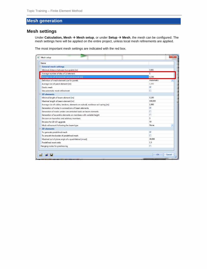
Mesh settings Under Calculation, Mesh � Mesh setup , or under Setup � Mesh , the mesh can be configured. The mesh settings here will be applied on the entire project, unless local mesh refinements are applied. The most important mesh settings are indicated with the red box.

Mesh generation

7

General mesh settings

Minimal distance between two points [m]

If the distance between two mesh nodes is lower than the value specified here, the two points are automatically merged into one single point. This option applies for both 1D and 2D elements.

Average number of tiles 1D element

If necessary, more than one finite element may be generated on a single beam. The value here specifies how many finite elements should be created on the beam.

This value is only taken into account if the original beam is longer than the adjusted Minimal length of beam element and shorter than the adjusted

Average size of 2D element/curved element [m]

The average size of the edge for 2D elements. The size, defined here, may be changed through refining the mesh in specified points.

This option also defines the magnitude of finite elements generated on curved beams.

Definition of mesh element size for panels

This applies only to load panels.

If the load transfer method for load panels is set to Accurate (FEM) , then a FEM analysis is performed to define the load transfer. By this setting the mesh size of such load panels can be defined.

Average size of panel element [m]

This applies only to load panels.

This option is only used when to option above is set to Manual .

Defines the average size of mesh elements for load panels.

Elastic mesh If this option is activated, then the mesh generator will assume that the segments of the mesh are elastic . This allows further maintenance of numerical stability in case of strong mesh refinements.

Use automatic mesh refinement

Only available if Elastic mesh is activated .

The mesh will automatically be refined based on a certain load case. The refinement happens on mesh generation after calculation (so only after generating the mesh after the linear calculation has already been done) until the target error is achieved.

Target error for mesh refinement [%]

Only available if Use automatic mesh refinement is activated .

When an already calculated project is meshed again, the mesh will be refined on certain positions until the target error is achieved.

Load case for mesh refinement

Only available if Use automatic mesh refinement is activated .

Automatic mesh refinements are done based on this load case. On the positions where peak results appear, the mesh will be refined.

Hanging nodes This applies only to post-tensioned cables .

Post-tensioned tendons will be calculated by placing at the real position of the tendons. The nodes are ‘hanging’ at a distance from the model.


8

1D elements

Minimal length of beam element [m]

When a beam of the structure is shorter than the value here specified, then the beam is no longer divided into multiple finite elements even though the parameter above (Average number of tiles of 1D element) says so.

Maximal length of beam element [m]

If a beam of the structure is longer than the value specified here, then the beam will be divided into multiple finite elements so the condition of maximal length is satisfied.

Average size of cables, tendons, elements on subsoil, nonlinear soil spring [m]

To obtain correct results, it is necessary to generate a much finer mesh on cables, tendons (prestressed concrete) and beams on subsoil.

Generation of nodes in connections of beam elements

If this option is ON, a check for "touching" beams is performed. If an end node of one beam "touches" another beam in a point where there is no node, then the two beams are connected by a FE node.

If the option is OFF, such a situation remains unsolved and the beams are not connected to each other.

The function has the same effect as performing the function Check of data .

Generation of nodes under concentrated loads on beam elements

If this option is ON, finite elements nodes are generated in points where the concentrated load is acting. This option is normally not required.

Generation of eccentric elements on members with variable height

This specifies the number of finite elements generated on a haunch. This option prescribes the precision of the modelling. The larger the number, the better the model approaches the reality .

Division on haunches and arbitrary members.

Finite elements will always receive a constant height, rigidity and cross-section. So haunches and arbitrary members must be divided into different finite elements according to this number.

Division for 2D-1D upgrade When performing the 2D-1D upgrade , this mesh setting will be used.

Mesh refinement following the beam type This specifies if the nodal refinements should also be applied on beam

members. The nodal refinement is represented by a volumetric element, namely a sphere. As a consequent, the mesh of all the structure elements situated in this sphere will be refined taking the following possibilities into account:

None The refinement is applied to 2D members only.

Beams and columns The refinement is applied to elements which have the type beam or columns, or a type of beam or column, but not to ribs for example.

All 1D members The mesh refinement is applied to all 1D members.

Mesh generation

9

2D elements

To generate predefined mesh

If this option is ON, the mesh generator first tries to generate a regular quadrilateral finite element mesh i n every slab complying with the adjusted element-size parameters. Only if required, additional needed nodes are added to the mesh.

If this option is OFF, the finite element mesh nodes are first generated along the edges and further, the mesh is generated to the middle of the plate.

Generally, the first option is faster, gives less 2D mesh elements and has a regular mesh in the middle of the plate. At the transition to an inclined edge the elements can be less optimal. The parameter ratio predefined mesh determines the distance (in relation to the element size) between the predefined mesh and the edges.

To smooth the border of predefined mesh

If this option is ON, the border elements of the predefined mesh are included into the process of smoothening, i.e. the mesh area consisting of regular quadrilaterals can be increased.

Maximal out of plane angle of a quadrilateral element [mrad]

This value determines whether a spatial quadrilateral element whose nodes are not in one plane will be replaced by triangular elements. This parameter is only meaningful for out-of-plane surfaces – shells. The assessed angle is measured between the plane made of three nodes of the quadrilateral and the remaining node of this quadrilateral.

Predefined mesh ratio Defines the relative distance between the predefined mesh formed by regular quadrilateral elements and the nearest edge. The edge may consist of an internal edge, external edge or border of refined area. The final distance is calculated as a multiple of the defined ratio and adjusted average element size

for 2D elements.


10

Mesh size 2D elements The correct mesh size is a vague concept. A finer mesh gives better results in general, but in case of singularities or peak values, a finer mesh makes these peaks much worse. In SCIA Engineer, the results on plates are by default already post-processed. This means that you see results that are a bit brushed up.

Model

The mesh size will be evaluated for the project Mesh_Size_2D.esa .

The project start with a mesh size of 1m for the 2D elements.

The loads in the project consist of only the self weight.

Results

The linear calculation is performed. When looking at the internal forces on the 2D element, the following results can be shown (under Results � 2D members � internal forces � mx)

Mesh generation

11

As mentioned before, these results are post-processed results. The post-processing configuration can be seen in the property ‘location’ . There are 4 choices for ‘location’ : More details can be found in annex 2.

1. In centres

This option will show the results averaged per finite element. The result will look like a mosaic.

2. In nodes, no avg.

This option gives the unchanged results, which originate directly from the solver. These can be called the ‘pure’ results.

3. In nodes, avg. This option will taken a parabolic average of results in each mesh node. This will make give a more fluid representation when showing the results.

4. In nodes, avg. on macro This option does the same as the option above, as long as the finite elements come from the same plate, wall or shell. Unlike the previous option, this one will not average results from a plate and wall for example.

It is clear that the results of the option ‘In nodes, no avg .’ must be investigated. We use a fixed palette so to have a better comparison of results.

The results are not alike, which means that the post-processing has quite a big impact on the representation of results. This indicates that the mesh is not fine enough.


12

Solution

A rule of thumb for concrete plates is to take a mesh size equal to 1 or 2 times the thickness of the plate. In this project that would be 1 or 2 times 0,2m for the wall, and 0,3 for the plate. Let’s take a mesh size of 0,25m. The unprocessed results now look like this:

While the processed results look like this:

The results with or without post-processing have a very similar presentation of results. This indicates that the mesh is fine enough. If necessary, it is also possible to use local mesh refinements. These can be found in the main menu under “Calculation, mesh � local mesh refinement ”.

Mesh generation

13

Elastic mesh In the project “Mesh_Elastic.esa” we are going to show the effect of using an elastic mesh.

Model

The model has the dimensions shown in the image below.


14

Results

First the mesh is generated without the elastic mesh. This can be set in the mesh settings:

The global mesh setting is 0,2m. The mesh can be generated by using Calculation, Mesh � Mesh generation , or in ‘Project’ toolbar

with the icon: The mesh can be displayed by the view parameters. These can in the graphical display bar under Set

view parameters for all > Structure > Mesh > Draw mesh. The elastic mesh in the mesh setup provides a fluent transition between mesh sizes.

Elastic mesh on (default setting):

Elastic mesh off :

Mesh generation

15

Automatic mesh refinement SCIA Engineer 14 offers a new feature - Automatic mesh refinement. A fine mesh of finite elements produces more accurate results than a coarse mesh. But to find the correct fine mesh is sometimes a very hard task for a user. Therefore, we are releasing this new method for automatic mesh refinement. This method has been developed in collaboration with our partners – FEM consulting s.r.o and Czech Technical University in Prague. Our solution reflects state of the art error estimation methods. The benefit of the method is also that now information is given about the quality of results due to the used mesh density of two-dimensional mesh elements.

Model

The model Mesh_Automatic.esa is composed of a ground and top, separated by multiple columns.

Results

As indicated in the example about mesh refinements, the mesh can be judged by going to a 2D result, and setting the ‘Location’ to ‘In nodes, no avg.’. In the image below, the moment mx has been asked for the self weight.

The mesh is certainly not good enough. You can see that there are incoherent results and peak values near the columns.


16

Solution Now we will perform an automatic mesh refinement based on the results for the self weight. To perform the automatic mesh refinement, the next steps are required.

1. Activate the automatic mesh refinement.

a. Go to the mesh settings.

b. Activate both elastic mesh and automatic mesh refinement.

c. Choose the load case and the target error for the mesh refinement.

2. Perform the linear calculation. You will also receive information about the error estimation for the load case configured in the previous step.

3. If desired, you can check the numerical error by going to the results menu and by checking “Num. Error, Mesh refinement” for the 2D elements.

4. To perform the automatic mesh refinement, you must manually click on the mesh generation. This option can be found under Calculation, mesh .

5. Now perform the linear calculation again. The estimated error will have reduced, since the mesh has been refined.

Mesh generation

17

6. To go even further in the mesh refinement, run through steps 4 and 5 until the desired result is achieved.

After just 1 mesh refinement, the mesh is now locally refined.

The unprocessed result for mx also shows less jumps.

To improve the results, we advise to also add averaging strips. This is treated in the chapter about singularities.


18

Singularities and peak values

1D elements are modeled as frames. The elements are represented by lines which are linked together in nodes. 2D elements are modeled as surfaces. The elements are represented by planes which are linked together over the edges. If a 1D member is connected to a 2D member in a single node, this can introduce problems. The 2D element will not be able to transfer all forces from the 1D element in just the node. This is what we call a singularity.

- Peak results will appear in the 2D element.

- The connecting node will seem to be partly hinged.

Nodal support - Averaging strips In most cases, a column or pole is introduced as a nodal support. The real dimensions of the support are neglected. In the Finite Element Method this is a singular node and the bending moment above this support is theoretically infinite. The moment will also converge to this infinite value with increasing mesh refinement. Refining of the mesh does not lead to the desired results in this case since the moment does not converge to the real value. A possible solution is to use averaging strips.

Model

A square slab is inputted with dimensions 2m x 2m in the model Singularities_AveragingStrips.esa. The mesh size is set to 0,25m and a surface load of 5kN/m² is inserted.

Results

After the calculation, the following results for mx in nodes not averaged are obtained: It is clear that peak values occur due to the reaction force of the nodal support. This peak value is correct and converges to the theoretical value infinity by increasing the mesh refinement.


19

Solution

An averaging strip will be added to take care of the peaks due to the reduced connection size of the analytical model. An averaging strip was inputted in the Y-direction with “Direction” set to “Perpendicular” and a width of “1m”:

Now the result of mx (in nodes, not averaged) with the averaging strip become:

By looking at the numerical results, a manual verification can be made. First we look at the averaged results.


20

For the same X-coordinate, in each element the same value will be obtained. Looking at the results in numbers without the averaging strip, the same value can be calculated taking the average of one line with the same X-coordinate within the averaging strip.

The -1,60 from the previous page can be found as: �0,41 � 1,33 � 1,84 � 2,78 � 2,78 � 1,87 � 1,36 � 0,458 � �12,828 � �1,6025


21

This averaging strip was defined as “Perpendicular” and inputted in the Y-direction. Looking at mx (perpendicular to the Y-direction) an average will be made. When we look at my (parallel with the Y-direction) no average will be made:

When changing this average strip from perpendicular to longitudinal, an average will be made for my but not anymore for mx.

Note : The averaging algorithm uses only the finite elements that are located inside the averaging strip.

This may cause certain inaccuracies especially in combination with larger finite elements. Therefore, it is recommended to define internal edges along the averaging strips . This ensures that finite element nodes are generated along the edge of the averaging strip, which may significantly improve the accuracy.

The recommended procedure is thus:

- Define the model of the structure

- Perform the calculation

- Review the results

- Define averaging strips

- Review the averaged results

- Decide the final location and number of averaging strips

- Define internal edges along the averaging strips

- Repeat the calculation to obtain the improved results


22

Nodal support – Subregions Instead of using averaging strips for plates supported by nodal supports or by columns, it is also a possibility to calculate this moment correctly by introducing the column not as a nodal support but as a flexible supported subregion. The dimensions of the subregion are the dimensions of the column. The flexible support can be calculated out of the stiffness of the column. The results of such an approach are compared to the results of a nodal support in the example below. With an element mesh of half the dimension of the column, the model with a subregion gives a good value of the occurring moment. The value is a little bit higher than the real occurring moment. An even finer mesh gives unreal values. An element size equal to the dimension of the column is too coarse and gives an underestimation of the real occurring moment.

Model

In this example (model Singularities_Subregions.esa ) a floor structure is analyzed. It is supported by columns with a distance of 6 m. The plate has a thickness of 0,2 m and is made of concrete C25/30 according to the EC. The whole is charged with a surface load of 100 kN/m². For the calculation one field of 6mx6m is considered. In the middle of this field a nodal support is inserted to represent the column. At the edges the rotation of the plate is prevented in both directions since the plate is stuck ‘on itself’. In the first case the column is introduced by means of a nodal support. Secondly, the column is made as a sub region supported by a flexible foundation. And in the last case, an averaging strip is used with the dimensions of the column. For the calculation of the stiffness a concrete column has been taken with a E-modulus of 32.000 MPa, height 4m and cross-section 0,5m x 0,5m.

33

2

800084000

32000

mMN

mmN

mmmm

N

h

Ek ====

Results

The results show the greatest peak value when the nodal support is used without an averaging strip. The moment is strongly reduced when a subregion has been used.


23

The structure is calculated with Mindlin elements. The results are claimed in nodes, averaging. The table below shows the maximal value of mx above the nodal support or the subregion.

Element size [m]

Nodal support

[kNm/m]

Elastic foundation

[kNm/m]

Averaging strip

[kNm/m]

1 -840,21 -459,56 -767,07

0,5 -1077,77 -491,40 -932,79

0,25 -1316,08 -693,83 -1030,88

0,125 -1556,74 -722,04 -1065,97

0,0625 -1796,93 -723,16 -1076,01

This table can also be plotted to show the convergence.

Conclusion

The buffering effect of the subsoil on the result is clearly noticeable. From this, you can conclude that the subsoil will approach the reality most accurately.

-2000

-1800

-1600

-1400

-1200

-1000

-800

-600

-400

-200

0

00,20,40,60,811,2

Mo

me

nt

mx

(k

Nm

/m)

Element size (m)

Nodal support [kNm/m]

Elastic foundation [kNm/m]

Averaging strip [kNm/m]


24

Rigid line supports A frequently occurring misunderstanding is the fact that the user thinks that a simple plate supported on 2 edges behaves as a beam. This is only the case without transverse contraction (if ν = 0). With normal values of the Poisson coefficient (ν = 0,2 or ν = 0,3) very high peaks of the reactions appear near the angles. Mesh refinement does not offer a good solution in this case and even increases the peak value. This peak value is correct and converges to the theoretical value infinity by increasing the mesh refinement. This can be explained as follows: Consider the plate as different beams which lie next to each other. With ν = 0,2, the bottom of the beam becomes smaller, the top on the other hand becomes broader. The plate is going to bend in a direction parallel to the supported edges, with the round side upwards (saddle forming: the plate deforms in the bearing direction with the round side upwards). This bending is prevented by the line supports. In a continuous plate this will cause bending moments my in the transverse direction, approximately with a size of 0,2 mx. If this moment my occurred along the entire width of the plate, the reaction would be constant. However, the moment has to be zero on the free edges. So, it seems that an opposite moment 0,2 mx exists on this edge, that which leads to great reactions in the corners. In other words: at the end of the plate the saddle forming is not prevented anymore by the moments in the plate. The plate wants to deform downwards at the end, which is prevented by the rigid supports. Because of this, very large reactions appear.

Model

In the example Singularities_PlateBeam.esa , a plate of 3mx10m is calculated according to EC. The material is made of concrete C25/30. The thickness of the plate amounts to 200 mm. The plate is supported on the long edges and is loaded by a uniform load of 100 kN/m2. Without the plate action a uniform line load of 150 kN/m is expected along each border.

Results

The plate is calculated with an increasingly finer mesh. The maximal reaction in the corner increases more and more. The image below shows the result for a mesh size of 0,1m.


25

Solution

The peak in the reaction can be attributed to the infinite stiffness of the support. A realistic stiffness reduces the peak value considerably. Assume that the rigid supports should represent a concrete wall with E-modulus 32.000 MPa, a thickness of 0,1m and a height of 4m. This wall would have a certain rigidity.

22

2

8008004000

100.32000.m

MNmm

Nmm

mmmm

N

h

tEk ====

By assigning this rigidity to the line supports, the peak value disappears and no longer poses a problem when refining the mesh.

Element size [m]

max. reaction rigid

support [kN/m]

max. Reaction flexible

support [kN/m]

Reduction peak

value %

0,8 179,62 175,28 2,42 %

0,4 232,84 204,93 11,99 %

0,2 326,44 225,16 31,03 %

0,1 438,90 231,95 47,15 %

0,05 549,06 233,67 57,44 %

This last table can also be represented in a graphical representation.

0

100

200

300

400

500

600

0,8 0,4 0,2 0,1 0,05

Max

imal

reac

tion

[kN

/m]

Element size [m]

Plate beam - effect flexible support

Rigid support

Flexible support


26

Connecting 1D and 2D members If a 1D member is connected to a 2D member in a single node, this can introduce problems. The 2D element will not be able to transfer all forces from the 1D element in just the node.

- Peak results will appear in the 2D element.

- The connecting node will seem to be partly hinged.

Example 1: Beams between walls

Model

When two walls are connected with a beam, this phenomenon can appear.

In the following example (“Singularities_1D_2D_Moment_Walls.esa ”), two walls with a dimension of 4x4 m are connected with each other by means of a beam with a length of 4m. This member is loaded in the middle through a point force of 10kN.

Even though the beam is fixed on both walls, it seems that it has a moment of zero at the connections. In other words, it looks like there are hinged connections. The beam seems to be hinged due to the fact that plates do not have a moment mz,, since torsion in the plane of a plate is always taken up by the normal forces nx and ny.


27

Solution

The solution exists in having 1D members connected to both the node and the edge of the 2D elements. These 1D members that do not really exist in reality are called ‘dummy members’. In this example, the result would look like this:

But since you are adding elements, and thus rigidity to the model, you must be able to explain why these elements are used. In the finite element model, the beam is only connected in the node. But in reality, the entire cross-section is cast and connected to the plate. So in reality, the beam is also connected to the wall over a certain region (and not in a single node). But as you can see in the image above, the dummy elements are much longer than the height of the cross-section, so what is the effect of the length of the dummy element? The table below shows the moments in the beam, as well as the rotation in the end nodes in function of the length of the dummy element.

Length dummy-beam (m)

Field moment Mz (kNm)

Moment at the ends Mz (kNm)

Fiz (mrad)

0,0 10,00. -0,00 0,278 0,2 6,41 -3,59 0,078 0,4 6,20 -3,80 0,067 1,0 6,18 -3,82 0,065

As you can see, a length of 0,4m is sufficient. The beam in our example has a cross-section height of 0,5m, which more than justifies the use of a dummy element with a length of 0,4m to 0,5m. The moment line in the beam is now very different:


28

Example 2: Plate on a single column

When a structure exists of a plate with a column on top of it, the user has to pay extra attention to this when there is a question of torsion. If the plate is subject to forces or moments, which cause torsion, very large deformations may occur. The thought behind it is the lack of a degree of freedom in SCIA Engineer, namely the rotation around the z-axis. In other words, the moment mz cannot be claimed when asking for the internal forces of a 2D element. The solution for this is the application of ‘dummy-members’ at the location of the connection between column and plate. This is clarified with the following example (“Singularities_1D_2D_Column_Plate.esa ”).

Model

Columns with a dimension of 500x500mm and a length of 4m are attached to a plate of 4x4m with a thickness of 500 mm. As load case, two point forces of respectively –1 kN and 1 kN are applied on the edge nodes of the plate. These forces are lying according to the global X-axis. In this way, the plate will be subjected to a rotation in his own surface without any transformation of the geometry.

Results

When the global deformation in the plate is examined, very large deformations seem to appear. This is especially the case at the location of the edges. The displacement at the center is zero. This indicates very clearly that the plate rotates around the connection with the column.


29

This phenomenon can be ascribed to the fact that the plate has no rotational stiffness around the Z-axis. ‘Energyless’ deformation occurs, which means that the plate does not know any resistance against the deformation��.

Solution

Dummy elements

The top of the column must be connected to the plate with more than just a node. By applying small horizontal beams over the top of the column, it is possible to connect the edges of the finite plate elements to the top node of the column.

After applying these dummy elements over the top of the column, it is remarkable that this deformation will be much smaller and nearly equal to the deformations of the plates on which the dummy-members are fixed. This means that an infinite rigidity is ascribed to the connection plate-column. You can verify this by comparing the deformation of this node in the plate with the deformation fix of the column:

Applying two crossing dummy-members at the connections is a way to get a correct approach of the reality. These are attached to the plate by means of internal edges. This way, the small beams will take the rotation of the plate on themselves, so the plate has a stiffness around the Z-axis. In this case, the large deformations at the edges will be gone.


30

In the example, a variation of the length of the beams is applied to verify the influence on the deformations. With this you receive the following results with a constant mesh of 0.25 m:

Length of dummy [m]

qxy max [kN/m]

Fiz max [mrad]

Ux max [mm]

0,00 57,54 -0,330 24587,5030,05 145,83 -0,145 0,412 0,10 38,08 -0,152 0,332 0,15 23,52 -0,151 0,313 0,20 13,21 -0,154 0,306 0,25 10,63 -0,154 0,303 0,35 6,12 -0,155 0,299 0,50 3,55 -0,156 0,297 0,75 1,80 -0,157 0,297 1,00 1,78 -0,157 0,297

Several conclusions can be drawn:

• When applying members of a very short length , this will affect the rotation and deformation sufficiently .

• Increasing the length of such a dummy-member will only have a small influence on the deformation and rotation.

• The shear stress qxy on the other hand, has a larger influence when increasing the length: the larger the beams, the smaller the shear stress in the plate.

• The shear stress varies little when a length of approximately half the section of the column is taken

• When using a length of the same dimensions as the section of the column , plausible results can be expected.

• The section of the beams has a significant influence on the shear stress: a greater section gives rise to a smaller shear stress and reverse.

� Preparatory to an analysis, a width equal to the dimension of the column and a height equal to the thickness of the plate can be considered.

Mesh size Subsequently the size of the mesh is varied when using a constant length of the dummy-beams, namely 0,25 m. The following results can be summarized in a table:

Mesh Size [m]

qxy max [kN/m]

Fiz max [mrad]

Ux max [mm]

1 3,79 -0,147 0,301 0,5 7,66 -0,149 0,301 0,25 10,63 -0,154 0,303 0,125 15,06 -0,164 0,304 0,1 14,44 -0,173 0,304 0,05 25.74 -0,193 0,305 0,025 39.60 -0,242 0,305

Also here following conclusions can be drawn:

• The deformation and rotation are only influenced with the size of the mesh to a limited extent.

• The shear stress has a larger influence: it increases as the size of the mesh decreases. � Preparatory to an analysis, a mesh equal to the length of the beam or the double of the length can be taken, depending on the thickness of the plate.

Eccentricity

31

Eccentric elements

Eccentric column

Model

In this chapter the effect of eccentricities is discussed. As an example, we have constructed a simple frame in a frame XZ environment (“Eccentricity_column.esa ”).

• The columns are 3m high.

• The beam is 4m long.

• All elements have a cross-section 300mm x 300mm (made of C25/30).

• A line load of 5kN/m is applied on the beam.

An eccentricity can be introduced on 2 ways

• By changing the “Member system line at” option.

• By introducing a value for ey and/or ez. It is not surprising that several possibilities have the same effect. For example this example, we set “Member system-line at” “bottom”, which would be the same as inputting ez = 150mm (height cross-section divided by 2). So for this example:

=


32

Results

When looking at the moment diagram, we can notice some odd results

• The results are non-symmetrical.

• The moment at the bottom of the left column is not zero, although the support is hinged.

• The moment at the top of the left column is not equal to the moment on the left of the beam.

When looking at the normal forces, there is nothing strange at all. Both columns take 10 kN compression force of the line load of 5 kN/m over the 4m long beam.

The increased moment on the left column is due to the eccentricity which has been applied. The additional moment can be calculated as: ∆�� ∗ �� 10�� ∗ 0,15� � �1,5�� This explains the moment of –5,56 kNm: �� ,�� ∗ � � �4,06�� !�10��" ∗ 0,15� ��4,06�� 1,5�� 5,56��

Eccentricity

33

Interpretation

Why do we add the extra moment?

• In SCIA Engineer, the results are always shown for the neutral axis of the element.

• The connections between elements, supports, etc are made in nodes, as required in a finite element model. The nodes are always at the ends of the system lines.

• So if an eccentricity is applied, the neutral axis will no longer be the same as the system line. The recalculation of internal forces from the system line towards the neutral axis is what causes the jump in the moment line (from -4,06 kNm to -5,56 kNm). This is also represented in the image below.

• The first column on the left is the same as you can see it in SCIA Engineer (the light blue line is added, representing the neutral line).

• But in fact, you should represent an eccentric element as if the eccentricity is applied by small horizontal elements. This is represented in the middle image.

• When you look at the internal forces of an element, these internal forces are always applied to the neutral line of the specific element. In this case, it implies that the forces in the nodes (coming from the beam and support) should be recalculated to the blue line. The recalculation is added to the third image (on the right).


34

The same principle can also be shown by creating small stiff beams. To do this, we have used a cross-section 3000x3000 (=’very high stiffness’), which we have converted to a numerical cross-section.

Eccentricity

35

Eccentric beam

Model

In this example the effect on normal forces due to eccentricities is discussed. As an example, we have constructed a simple beam in a frame XZ environment (“Eccentricity_beam.esa ”).

• The beam is 6m long.

• All elements have a cross-section 500mm x 300mm (made of C25/30).

• A line load of 10kN/m is applied on the beam.

• The eccentricity is inputted with “member system-line at”: “bottom” (or � � 150��)

As you can see, the line load is inputted on the beam and follows the eccentricity of the beam. The supports are in the nodes, which are positioned eccentrically from the neutral line of the beam.

Results In the results, you might notice some results which you intuitively would not expect:

• There is a normal force (although only a line load perpendicular to the beam was applied).

• The begin and end moments are not zero, although the supports are hinged .


36

Interpretation

First let’s run over the effect of bending without the eccentricity involved.

No eccentricity

The results in SCIA Engineer for this same case (without eccentricity) would be:

• The top fibres are in compression

• Due to a line load of 10kN/m over a length of 6m, the maximal moment would be:

��,�#$ � % You can see this corresponds perfectly with the result shown above. The difference in sign is merely a difference in convention used by

• Due to this moment, the bottom fibre is compressed and will become shorter.

• The bending stress is zero in the middle of the beam (= the neutral axis).

• The bottom fibres are in

Finite Element Method

n over the effect of bending without the eccentricity involved.

Engineer for this same case (without eccentricity) would be:

compression due to the bending stress. So they also become shorter.&'��(��) � �� ∗ *+ � , ∗ - Due to a line load of 10kN/m over a length of 6m, the maximal moment would be:

∗ ./8 � �10�� ∗ !6�"/8 � �360��8 � �45��

You can see this corresponds perfectly with the result shown above. The difference in sign is merely a difference in convention used by SCIA Engineer.

Due to this moment, the bottom fibre is compressed and will become shorter.

The bending stress is zero in the middle of the beam (= the neutral axis).

s are in tension due to the bending stress. They would become longer.

due to the bending stress. So they also become shorter.

Due to a line load of 10kN/m over a length of 6m, the maximal moment would be:

Due to this moment, the bottom fibre is compressed and will become shorter.

due to the bending stress. They would become longer.

Eccentricity

37

With eccentricity

Due to the eccentricity, the supports are at the position of the bottom fibres (in the circles in the next image). These bottom fibres would normally become longer due to bending, but the supports do not allow these displacements.

As a result, the supports force the elongation at the bottom fibre to be zero by means of a reaction force. This can also be seen in the results.

• The reaction force 0$ from the supports introduces a normal force in the beam. This is a constant normal force of -90 kN over the beam.

• Due to this reaction force, there will be no elongation at the bottom fibre.

• And due to this reaction force at an eccentricity ��, the moment line is shifted. Δ� � � ∗ �� 90�� ∗ 0,25� � �22,5��

This causes the moments at the begin points to be -22,5 kNm and the maximal moment to be shifted up from 45kNm to 22,5kNm.


38

Ribs

Introduction By means of the menu Structure > 2D element components> Rib a plate can be stiffened with members. A rib is calculated as a beam with eccentricity with regard to the axis of the plate. The member elements are connected to the plate at the height of the mesh nodes. In a 3D General project, the rib can be placed below, in the middle or above the plate. A rib that lies below or above the plate causes membrane forces in the plate. In SCIA Engineer a rib below a plate is always shear resistant connected to the plate. The total rigidity is according to the rule of Steiner:

Rigidity beam + Rigidity plate + Surface beam x (axis-distance-beam-plate)². So it is important to realize that also in reality the beam and the plate have to be connected shear resistant to each other. If it is about a prefab construction at which the plate is on the beam, then the beam has to be placed in the middle of the plate in the calculation model. The effective width of the rib is calculated implicitly by the behaviour of the finite elements under membrane forces during the Finite Elements Calculation. In the following view of the membrane forces nx in the longitudinal direction of the beam, the effective width is clearly noticeable.

The section of the rib can be shown graphically, in that way you can see if the effective widths overlap each other or not. This can be done by means of view parameters, by using ‘Set view parameters for all > Structure > Draw cr oss-section’.

Ribs

39

Forces in rib What is explained in the previous paragraph also counts for a member that is connected to a plate and is aligned eccentrically by an Internal edge . The difference with a plate rib is that for a rib an Effective Width can be inserted too. The Effective Width was specifically implemented to follow the code concerning the calculation of the theoretical reinforcement. Because when the option Rib is marked with the results, a replacement T-section is used to calculate the results. The height of the T-section is determined by the height of the beam + the height of the plate . The flange width of the T-section equals the entered Effective Width. The internal forces for the replacement T-beam are calculated as follows:

The coordinates of the hearts are used as lever arms in the Y and Z direction:

Lever arm Z1 = T1z – Tz Lever arm Y1 = T1y – Ty Lever arm Z2 = T2z – Tz Lever arm Y2 = T2y – Ty Lever arm Z3 = T3z – Tz Lever arm Y3 = T3y – Ty Lever arm Z = Tz – 0z Lever arm Y = Ty – 0y

- N = N beam + N plate, left + N plate, right

- Vy = Vy beam + Vy plate, left + Vy plate, right

- Vz = Vz beam + Vz plate, left + Vz plate, right

- Mx = Mx beam + Mx plate, left + Mx plate, right

- My = My beam + My plate, left + My plate, right + N plate, left * (Lever arm Z1) + N plate, right * (Lever arm Z2) + N beam * (Lever arm Z3)

- Mz = Mz beam + Mz plate, left + Mz plate, right + N plate, left * (Lever arm Y1) + N plate, right * (Lever arm Y2) + N beam * (Lever arm Y3)

If the option Rib is activated when claiming the plate forces, the internal forces in the cooperating width of the rib are equated with zero. This counts for the internal forces in the longitudinal direction of the rib. The forces perpendicular to the rib remain unchanged. These internal forces can be equated with zero for the reinforcement calculation because they are taken into the reinforcement calculation of the rib. And so the whole plate-beam is replaced by a T-beam. However, note that when using several ribs below a plate element, the cooperating widths of this cannot overlap each other. If this does happen, the values of the internal forces are charged double on the spot of the overlapping parts.

T the heart of the entire replacement T-section T1 the heart of the left part of the effective width T2 the heart of the right part of the effective width T3 the heart of the original rib


40

Model

In the project Rib_vs_T.esa a beam is calculated with a length of 10m and concrete quality C25/30 according to EC. The beam is supported at the extremities, loaded with a distributed load of 200kN/m and has following section:

The beam is modelled in 3 different ways:

- As member element

- As plate with a thickness of 200mm and with a rib of 200mm x 400mm below the plate

- Entirely with Finite Elements

Results

In the results you can see that the same bending moment is achieved by using a rib and a plate when comparing to a beam with a T-section. However, this result is achieved when the option ‘rib’ is ticked on.

If the option ‘Rib’ is ticked off, then the rib will show a very different result.

H 6

00

B 1000

th 2

00

sh 200

z

y

Ribs

41

Solution

When the option ‘Rib’ is ticked on, it means that the internal forces of the rib and its effective width must be combined. If the option ‘Rib’ is ticked off, only the stresses in the rib are combined to the internal forces.

It is also possible to check how the internal forces of the rib and the plate are combined. If the option Rib is off, then you will have the next internal forces in the rib. These forces apply to the center of the rib, T3.

The internal forces in the plate can be found by a section on the middle of the plate, over the width. Then the averaged results over this section can be found.

These results apply to the centre of T1 and T2 together.


42

To find the internal forces in the rib with effective width, these two tables must be combined. �3 � �4�5��6�#�� !6216,26��" � !�6215,99��" � 0,27�� 7�,3 � 7�,4�5 � 7�,6�#�� !0,00��" � !0,00��" � 0,00�� ,3 � ��,4�5 ��,6�#�� 4�5 ∗ 8*3 � *39:;< � �6�#�� ∗ !*3 � *3=>?@A" As you can see, in the calculation of the combined moment, we take into account the centre of gravity of the entire T section to take into account the normal forces in the plate and the beam. The recalculated forces are thus to be applied on a different centre of gravity then the centre of gravity of the rib or the plate.

*3 � *39:; ∗ B4�5 � *3=>?@A ∗ B6�#��B4�5 � B6�#�� C0,4� 2D E ∗ 0,4� ∗ 0,2� � C0,4� � 0,2� 2D E 0,2� ∗ 1,00�0,4� ∗ 0,2� � 0,2� ∗ 1,00�� 0,016�³ � 0,100�³0,08�² � 0,20�² � 0,116�³0,28�² � 0,414286�

Now that the height of the centre of gravity of the combined section is known, the combined moment can be calculated. ��,3 � ��,4�5 ��,6�#�� 4�5 ∗ 8*3 � *39:;< � �6�#�� ∗ C*3 � *3=>?@AE� 388,89�� 246,10�� !6216,26��" ∗ !0,414� � 0,200�" � !�6215,99��"∗ !0,414� � 0,500�"� 388,89�� 246,10�� !6216,26��" ∗ !0,214�" � !�6215,99��" ∗ !�0,086�"� 634,99�� 1332,056�� 532,899�� 2499,845��

When we ask for the internal forces in the rib, with the option rib activated, the same results are shown.

Mindlin vs Kirchhoff

43

Mindlin versus Kirchhoff

Shear force deformation For the bending behavior of plates, there are 2 types of bending theories implemented:

- The Mindlin element including shear force deformation

- The Kirchhoff element without shear force deformation

With the Kirchhoff theory , a plane section of the plate remains perpendicular to the deformed axis of the plate in the deformed state. This traditional bending theory is applied for thin plates and is supported by following assumptions (ref .[1]):

- The middle plane is free of strains and stresses

- The stress component perpendicular to the surface (σz) is negligible (σz ≅ 0)

- Normal stresses on the middle plane also remain perpendicular to the reference surface after the deformation (hypothesis of Bernoulli)

For this theory the following conditions have to be satisfied:

- The thickness t of the plate is small with regard to the span L (t/L < 1/5 )

- The deflections w remain small in comparison to the thickness of the plate t (w/t < 1/5 )

On the other hand, the Mindlin theory doesn’t have all of the above-mentioned assumptions. The normal stresses on the middle plane remain straight but not necessarily perpendicular to the middle plane after deformation. As a consequence, additional strains γxz and γyz arise in case of a Mindlin element. This is shown on the picture below.

a) Represents the used symbols.

b) Shows the Kirchhoff element.

c) Demonstrates a Navier balk, which corresponds to the Kirchhoff element.

d) The Mindlin element.


44

The choice between these two elements can be made using the menu function Calculation, mesh > Solver setup . Default the Mindlin theory is used and because of this, special attention has to be paid to the use of thin plates.

This option is only in relation with 2D elements. Specifically for beams, the shear force deformation can be taken into account or not by means of the option Neglect shear force deformation (Ay, Az >> A) . The influence of the shear force deformation is especially important with thick plates with a small span.

Model

In the example MindlinKirchhoff_ShearDeformation.esa , a plate of 2m by 5m is supported at the shortest edges and made of concrete C25/30 according to EC. The thicknesses are 300mm, 600mm and 1200mm (from left to right). Surface loads of -150 kN/m2, -1200 kN/m2 and -9600 kN/m2 are applied. The mesh setting for finite element plates is set to 0,5m.

Results

The deflection in the middle of the plate:

Kirchhoff element Mindlin element % difference

Plate 300 mm -17.49 mm -17.01 mm 0.5 %

Plate 600 mm idem -18.47 mm 3.2 %

Plate 1200 mm idem -19.24 mm 13.7 %


45

Kirchhoff versus Mindlin on the edge of an element In the theory of Mindlin three degrees of freedom are available on the edge of a plate element:

o H = deformation in the local z-direction of the plate

o �I = rotation around ny (rotation parallel with the edge)

o �II = rotation around nx (rotation perpendicular on the edge) In Kirchhoff’s theory only two variables are needed, the variable does not exist, because shear deformation is not taking into account in Kirchhoff’s theory. On the edge, the following forces will be taking into account for Kirchhoff and Mindlin:

Kirchhoff Mindlin


46

Kirchhoff assumes a constant torsional moment on the end of the plate. At Mindlin’s theory, the torsional moment mxy will become zero on the edge, but this results in high values for vx. In Mindlin’s theory the torsional moment will go from its maximum to zero over a distance of t/2 (t = the plate thickness). For thin plates, this is a very small area, so when using Mindlin’s theory for thin plates a lot of finite elements will be necessary on the edges. This is shown in the following example.

Model

This next example (MindlinKirchhoff_edges.esa ) shows two plates with different thicknesses (200mm and 2250mm). The mesh of this plate is 0,5m, but on the edges a denser mesh has been inserted:

Results

The results on the thin and tick plates for both the Kirchhoff and Mindlin theory for different mesh sizes, are displayed in the table below (for the forces, the averaged results in nodes are taken).

Thin (200mm) Thick (2250mm)

Element size

edge [m]

Uz

[mm]

max |mxy|

edge

[kNm/m]

max. |vx|

edge

[kN/m]

Uz

[mm]

max |mxy|

edge

[kNm/m]

max. |vx|

edge

[kN/m]

Kirc

hhof

f

0,5 -6,191 15,00 15,53 -0,004 15,00 15,53

0,2 -6,184 15,03 16,35 -0,004 15,03 16,35

0,1 -6,190 15,04 15,19 -0,004 15,00 15,19

0,05 -6,190 15,04 16,69 -0,004 15,04 16,69

0,03 -6,190 15,03 17,53 -0,004 15,03 17,53

0,015 -6,190 15,04 21,37 -0,004 15,04 21,37

Min

dlin

0,5 -6,314 14,75 212,62 -0,007 9,37 18,86

0,2 -6,319 14,82 217,38 -0,007 9,75 18,96

0,1 -6,328 14,82 218,54 -0,007 9,79 18,90

0,05 -6,335 14,86 226,93 -0,007 9,80 18,92

0,03 -6,339 14,84 228,42 -0,007 9,80 19,12

0,015 -6,340 14,85 218,68 -0,007 9,80 19,15


47

Interpretation

Uz

The deformation Uz for Mindlin and Kirchhoff in the middle of the plate will be the same and will not depend on the border mesh size.

Mxy

Normally, the Mindlin theory would result in zero mxy using small elements. The comparison between Mindlin and Kirchhoff is made in the diagram below for the thin plate . It clearly shows us that for thin plates, there is no real difference in the result for mxy by using the Mindlin or Kirchhoff theory.

The comparison for the tick plate shows that when the calculation is done with Mindlin, mxy reaches lower values, even with a rougher mesh size (a mesh of 0,5m).

0,00

2,00

4,00

6,00

8,00

10,00

12,00

14,00

16,00

0,5 0,2 0,1 0,05 0,03 0,015

mx

y [

kN

m/m

]

mesh size [m]

Mindlin

Kirchhoff

0,00

2,00

4,00

6,00

8,00

10,00

12,00

14,00

16,00

0,5 0,2 0,1 0,05 0,03 0,015

mx

y [

kN

m/m

]

mesh size [m]

Mindlin

Kirchhoff


48

Vx

When looking at vx for the thin plate, the small values for vx at Kirchhoff’s calculation can clearly be seen, even with a small number of elements. But the Mindlin theory only gives high values for vx.

In this case, calculating with Kirchhoff is a better option, because Mindlin does not give good results, unless you would use an unrealistic small mesh along the border. When investigating the thick plate, it is clear that vx remains very small for Kirchhoff, and also Mindlin gives good results for vx. So for thick plates, calculating with Mindlin will give the best results, because shear force deformation.

0,00

50,00

100,00

150,00

200,00

250,00

0,5 0,2 0,1 0,05 0,03 0,015

vx

[k

N/m

]

mesh size [m]

Mindlin

Kirchhoff

0,00

5,00

10,00

15,00

20,00

25,00

0,5 0,2 0,1 0,05 0,03 0,015

vx

[k

N/m

]

mesh size [m]

Mindlin

Kirchhoff


49

Conclusion

Thin plates

• Calculating with Kirchhoff gives the best results for thin plates

• Using Mindlin a lot of elements will be necessary to obtain good results.

• Using Kirchhoff, the size of the elements do not have to be smaller than the plate thickness.

Thick plates

• Calculating an isotropic, homogeneous plate, Mindlin will be necessary

• On the edge a denser mesh will be necessary (more than 5 elements over the half of the plate thickness)

• Mindlin will also give good results for thin orthotropic plates with a small shear stiffness


50

Orthotropic properties in plates

The topic ‘orthotropic properties’ is available in the Concept Edition of SCIA Engineer.

Isotropic plate versus ‘1-direction’ plate

Model

The model Orthotropy_1direction.esa is used to show the difference between an isotropic and orthotropic plate. The orthotropic plate will be modeled to transfer loads through bending in only one certain direction.

The behavior of the plate will be investigated by checking how the load is transferred to the supports. In most use cases, the structure will transfer loads from the plate to the beams, and then from the beams to the supports. This behavior will be checked in the following steps. There is only 1 load case taken into account. In this line load, the separated beam will receive the same amount of load as what would be expected in the models with the plates.

As the plates are 6m x 6m, and the surface loads are 1kN/m², the load transferred to the beams should be around 3kN/m.

Orthotropic properties

51

Now the orthotropic properties will be applied. This can be done by selecting the 2D element, and changing the FEM model property to orthotropic. A new property will appear: “Orthotropy”.

In OT1 (orthotropic properties), the option 2 heights will be chosen. This allows both the flexural and membrane strengths to be configured with height parameters. The ‘1’ direction corresponds to the x-axis of the Local Coordinate System of the plate, the ‘2’ direction corresponds to the y-axis (which can also be derived from the explanatory image below).


52

Results

The linear calculation is performed. We look at the moments in the beams to see how loads have been transferred. In this result, you can see that the moment in the beam is practically the same for the single beam and the beams with the orthotropic plate.

Interpretation

The difference between the isotropic and the orthotropic element is (obviously) caused by the orthotropic properties. The isotropic plate also has capacity to deviate the load towards the support.

Thus the transverse bending stiffness of the isotropic load reduces the amount of load which would be sent to the beams.

Orthotropic properties

53

This effect can also be visualised in the following manner. Isotropic plates have equal strength in all directions. So in relation to the stiffness of the plate, it will send loads directly to the support instead of to the beam, when close enough to the supports.

This effect would even become more dominant if the stifnesses are higher. To show this, the thickness is doubled in both the orthotropic and isotropic plate. To do this, the OT1 setting is changed, and the properties of the isotropic plate are changed. This is also saved in the project Orthotropy_1direction_thicker.esa .

Now the beams along the isotropic edge have to take even less load, since the isotropic plate has higher bending stiffness in the y-direction. This allows the isotropic plate to transfer a bigger part of the load directly to the supports.


54

Pressure only

The topic ‘pressure only’ is not available in the Concept Edition of SCIA Engineer. The license code is esas.44 and it is only part of the Professional or Expert Edition .

When using pressure 2D elements, the functionality Nonlinearity and Pres only 2D members must be activated. The 2nd order – geometric nonlinearity functionality is also important as it allows us to use the Newton-Rhapson solver.

With this option, tension in 2D elements can be automatically eliminated. This is mostly used for masonry elements. When using this functionality, it is advised to adjust some parameters to smoothen the calculation. This will be treated in the next examples.

Masonry wall with window

Model

The model PressureOnly1.esa is used to show the difference between an isotropic and linear calculated wall (on the left) and a pressure only calculation (on the right).

Pressure only

55

Since a pressure only wall cannot take any tension, there are beams added over the opening to take the tension in that position.

To indicate which walls are calculated as pressure only, it is possible to assign the ‘Press only’ property to the FEM nonlinear model setting.

To calculate this non-linear setting, the non-linear calculation must be done. This requires non-linear combinations. Since a non-linear combination is non-associative, loads must be combined before the calculation, as opposed to the linear calculation. And thus non-linear combinations are required.

Now before starting the calculation, we will first run over the solver and mesh settings. This is very important in a pressure only calculation.

In the solver settings: - The maximum iterations is set to 100. - The Geometrical nonlinearity solver is set to Newton-Raphson . - We allow the solver to us 4 iterations . - The solver precision ratio is reduced to 0,25.

When the calculation is performed, the elements which take tension will have their rigidity reduced in the direction of the tension stress. The rigidity is reduced uniformly in that direction for the entire finite element. For this reason, the mesh must be sufficiently fine (in this example 0,150m is used).


56

Results

The non-linear calculation is performed. This calculation will modify stiffnesses in the press only wall until tension is sufficiently reduced or until the maximum number of iterations is achieved. The difference between the isotropic and the pressure only elements can be clearly view looking at the normal force n1 for these members. This result can be found under 2D member – Internal forces by setting the Type of forces to Principal magnitudes . After this, n1 can be chosen as value.

Interpretation

By asking the results as prinicipal magnitudes, the user can ask the biggest normal force (not in the x-direction, but in the direction with the biggest value). The biggest normal force means the most tension. As n1 is zero for the plate on the right, it is confirmed that all tension is removed from the wall. In the results of only the wall on the right, it is also clear to see that n1 (the normal force in the direction which has the biggest normal stresses and no shear stresses) is practically zero or negative. This also confirms that the used precision criterion in the solver settings is sufficient.

Pressure only

57

Cantilever with ribs as reinforcement When looking at the pressure diagonals in a reinforced 2D concrete element, ribs can be imported as reinforcement.

Model

In this example PressureOnly2.esa , a plate with a bearing support is inserted with three ribs acting as the reinforcement of the plate.

Calculation

In the non-linear calculation, the solver can indicate that the structure is instable if the reinforcement ribs are too weak for example, or if the wall cannot take the loads without inducing tension. To investigate the problem, you can choose to continue with the calculation. This allows you to see the results with which the non-linear solver has stopped. If the calculation has been performed, the status window shown on the right will become visible. It is clear that the non-linear calculation has found much bigger displacements than the linear calculation.


58

Looking at the results of this 2D element, the pressure diagonals inside this element are clearly visible (after changing the panel settings):

Ribs

59

Annex 1: Calculation of Rx in eccentric beams

Input Cross section = 300mm x 500mm Material = C25/30, with E = 31500MPa Line load = -10kN/m Length of the beam = 6m

Calculation

Formula of elongation

The total elongation is the sum of all the elongations at all the different positions on the beam. Such a sum can be calculated by integration.

• We want to integrate the elongation over the length of the beam.

• The elongation can be calculated from the stress.

• The stress can be calculated from the moment.

J -!K"LKMN � J &!K", LKM

N � ��!K" ∗ *, ∗ + LK

Moment line

So to calculate the elongation, we need to know the moment line in function of the position on the beam. This bending moment is a parabola in function of x (the position on the beam). If there is no eccentricity, then the result would look like this:


60

Now to compose the parabolic function: �� O ∗ K² � P ∗ K � Q We know about 3 points of this parabola:

R+SK � 0� Tℎ�V�� 0��+SK � 3� Tℎ�V�� 45��+SK � 6� Tℎ�V�� 0��W We can compose the following set of equations:

• X 0 � O ∗ 0/ � P ∗ 0 � Q�45 � O ∗ 3/ � P ∗ 3 � Q � 9O � 3P0 � O ∗ 6/ � P ∗ 6 � Q � 36O � 6P W •

We can derive from these equations that:

X O � 5P � �30Q � 0 W Resulting in: �� 5K² � 30K

Calculation of the total elongation

As mentioned before, the total elongation of the bottom fibre due to the bending moment can be calculated by


N � J ��!K" ∗ *, ∗ + LKMN

This elongation must is countered by a reaction force in the support. But in exchange, this reaction force causes an additional moment and an additional normal stress. So we can rewrite the equation above as:


N � J 8��!K" � RZ ∗ e\< ∗ *, ∗ + � 0$B ∗ , LKMN � 0

J 8��!K" � RZ ∗ e\< ∗ *, ∗ + � RZB ∗ , LKMN � J !5K² � 30K � RZ ∗ ��" ∗ !�ℎ/2", ∗ + � RZB ∗ , LKM

N� � ℎ2 ∗ , ∗ + J !5K² � 30K � RZ ∗ ��"LK � J RZB ∗ , LK^N

^N

� � ℎ2 ∗ , ∗ + ∗ _5K³3 � 15K² � e\RZ ∗ xaN^ � bRZ ∗ xcN̂B ∗ ,

� �0,5�2 ∗ 31500�dO ∗ 0,3� ∗ !0,5�"³12 ∗ ef5 ∗ !6"g3 � 15 ∗ !6"/ � 6 ∗ 0,25 ∗ RZh � 0i��²

� 6m ∗ RZ0,5m ∗ 0,3m ∗ 31500MPa� �0,5�2 ∗ 31500�dO ∗ 0,003125�n ∗ !360 � 540 � 1,5 ∗ RZ"��² � 6m ∗ RZ0,15m² ∗ 31500MPa� �0,5�196,875��² ∗ !�180��² � 1,5 ∗ RZ ∗ Nm²" � 6m ∗ RZ4725MN� 90�� 0,75�0$196,875�� 6m ∗ RZ4725MN � 24 ∗ 90�� 24 ∗ 0,75� ∗ 0$ � 6� ∗ 0$4725�� 0

Or, it can be simply concluded that: 24 ∗ 90�� 24 ∗ 0,75� ∗ 0$ � 6� ∗ 0$ � 0 24 ∗ 90�� 18 ∗ 0$ � 6 ∗ 0$ � 0 0$ � �90��

Annex

Annex 2: “Location”, the post

During a calculation in SCIA Engineer, the node deformations and the reactions are calculated exactly (by means of the displacement method). The stresses and internal forces are derived from these magnitudes by means of the assumed basic functions, and arealways less accurate. The Finite Elements Mesh in SCIAelement 3 or 4 results are calculated, one in each node. When asking the results on 2D memberoption ‘Location’ in the Properties window gives the possibility to display these results in 4 ways.

A. In nodes, no average

All of the values of the results are taken into account, there is no averaging. In each node are therefore the 4 values of the adjacent mesh elementsan indication that the chosen mesh size is too large.This display of results therefore gives a good idea of the discretisation error in the calculation model.

B. In centres

Per finite element, the mean value of the results in the nodes of that element is calculated. Since there is only 1 result per element, the display of isobands becomes a mosaiccurve with a constant step per mesh e

C. In nodes, average

The values of the results of adjacent finite elements are averaged in the common node. Because of this, the graphical display is a smooth course of isobands. In certain cases, it is not permissible to average the values - At the transition between 2D members

“Location”, the post -processing of results

Engineer, the node deformations and the reactions are calculated exactly (by means of the displacement method). The stresses and internal forces are derived from these magnitudes by means of the assumed basic functions, and are therefore in the Finite Elements Method

SCIA Engineer exists of linear 3- and/or 4-angular elements. Per mesh element 3 or 4 results are calculated, one in each node. When asking the results on 2D memberoption ‘Location’ in the Properties window gives the possibility to display these results in 4 ways.

All of the values of the results are taken into account, there is no averaging. In each node are therefore adjacent mesh elements shown. If these 4 results differ a lot from each other, it is

an indication that the chosen mesh size is too large. This display of results therefore gives a good idea of the discretisation error in the calculation model.

ment, the mean value of the results in the nodes of that element is calculated. Since there is only 1 result per element, the display of isobands becomes a mosaic. The course over a section is a curve with a constant step per mesh element.

The values of the results of adjacent finite elements are averaged in the common node. Because of this, the graphical display is a smooth course of isobands.

In certain cases, it is not permissible to average the values of the results in the common node:At the transition between 2D members (plates, walls, shells) with different local axes.

61

Engineer, the node deformations and the reactions are calculated exactly (by means of the displacement method). The stresses and internal forces are derived from these

therefore in the Finite Elements Method

angular elements. Per mesh element 3 or 4 results are calculated, one in each node. When asking the results on 2D members, the option ‘Location’ in the Properties window gives the possibility to display these results in 4 ways.

All of the values of the results are taken into account, there is no averaging. In each node are therefore shown. If these 4 results differ a lot from each other, it is

This display of results therefore gives a good idea of the discretisation error in the calculation model.

ment, the mean value of the results in the nodes of that element is calculated. Since there . The course over a section is a

The values of the results of adjacent finite elements are averaged in the common node. Because of

of the results in the common node: with different local axes.

Annex 2: Post-processor “Location”

62

- If a result is really discontinuous, like the shear force at the place of a line support in a plate. The peaks will disappear completely by the averaging of positive and negative shear forces.

D. In nodes, average on macro

The values of the results are averaged per node only over mesh elements which belong to the same 2D member ánd which have the same directions of their local axes. This resolves the problems mentioned at the option ‘In nodes, average’.

Accuracy of the results

If the results according to the 4 locations differ a lot, then the results are inaccurate and the mesh has to be refined. A basic rule for a good size of the mesh elements, is to take 1 to 2 times the thickness of the plate.

Annex

63

Annex 3: Theoretical background of orthotropic prop erties

Theory

Strains and stresses

In a 3D model, the following components of deformations appear in each point (respectively the deformations according to the x-, y- and z-axes): p!K, q, *"r!K, q, *"H!K, q, *"

From these deformations the following strains can be calculated:

s �tuuuuvε$ε�ε�ε$�ε$�ε��xyyyyz �

tuuuuuuv Lp LKDLr LqDLH L*D0.5 ∗ |$�0.5 ∗ |$�0.5 ∗ |��xy

yyyyyz�

tuuuuuuuuv Lp LKDLr LqDLH L*D0.5 ∗ CLr LKD � Lp LqD E0.5 ∗ CLp L*D � LH LKD E0.5 ∗ CLH LqD � Lr L*D Exy

yyyyyyyz

The stresses in each point are:

& �tuuuuv&$&�&�&$�&$�&��xyyyyz

The stresses and strains are connected to each other, in the simplest case this connection is linear (Hooke’s law):

σ = D ε

D is a 6x6 matrix. The connection between stresses and strains is not based on assumptions, but describes the real physical behavior of the material. For that reason, this matrix is called the “constitutive” matrix.

Internal forces

In the analysis of a 2D plate, the stresses are replaced by internal forces, which we will indicate with the symbol ‘s’. These internal forces are known as the results of SCIA Engineer:

s = [smT, sb

T]

sm = [nx, ny, qxy]T for membrane forces

sb = [mx, my, mxy, qx, qy]T for bending

The components of the deformations that are used with a 2D plate are the deformation of the axis of the plate (w), the rotation on the x-axis (φx) and the rotation on the y-axis (φy).

w(x, y) = w(x, y, 0)

φx(x, y)

φy(x, y) With the Kirchhoff element the normal remains on the plate axis perpendicular to the plate axis. So there is a double connection between w and φ:


64

φy = -dw/dx

φx = dw/dy With the Mindlin element the shear force deformations γxz and γyz also occur:

φy = -dw/dx + γxz

φx = dw/dy + γyz

Relation between strains and internal forces

From these 3 components of the deformation the strain can be calculated in each point of the plate (with the usual assumption that an even cross-section remains plane). From this strain the stress can be calculated in each point of the plate by means of the constitutive matrix. Through integration of these stresses over the thickness of the plate, the internal forces that belong to the deformation can be calculated (for the full calculation is referred to ref. [2]). This gives the following connection for the membrane forces and deformations in the plane:

∗

=

xy

y

x

xy

y

x

ddd

ddd

ddd

q

n

n

γεε

332313

232212

131211

For bending components and deformations from the plane:

−

−

∗

=

•

•

yz

xz

xy

x

y

y

x

xy

y

x

DD

DD

DDD

DDD

DDD

q

q

m

m

m

γγ

ϕϕϕ

ϕ

)(

00

00

00

00

00

'

'

5545

4544

332313

232212

131211

‘means the derivative to x, •, means the derivative to y. ϕ'y en -ϕ•

x are curves.

Annex

65

In most textbooks the shear force deformation is neglected. Then:

ϕ'y = -d2w/dx2 = curve κxx

-ϕ•x = -d2w/dy2 = curve κyy

ϕ•

y - ϕ'x = -d2w/dxdy -d2w/dxdy = -2 d2w/dxdy = curve 2 κxy

The matrix for the bending effects is subsequently written as:

∗

=

xy

yy

xx

xy

y

x

DDD

DDD

DDD

m

m

m

κκκ

2332313

232212

131211

By dividing the membrane force components and the bending components, it is implicitly assumed that these components do not mutually influence each other. These stiffness matrixes do not only describe the physical behaviour of the material, but also the stiffness of a plate element. This is specified by the material, possibly different materials over the thickness (reinforced concrete, laminated plates) and by the geometry (ribs, …). In SCIA Engineer the following components are entered in this matrix:

d11, d22, d33 and d 12 D11, D22, D33, D44, D55, D12

D44 and D55 are added because Mindlin elements with shear force deformations are used. In many cases there are no simple formulas to calculate these stiffnesses. The orthotropic parameters can be calculated by means of following formulas:


66

for plate elements :

G13 and G23 are used for the calculation of the stiffnesses D44 and D55. These are the stiffnesses for shear force deformation. In some cases they cannot be calculated exactly. In that case it is advised to enter D44 and D55 much larger (1000 times larger) than the other stiffnesses. In this way you will neglect the shear force deformation. The influence of the shear force deformation is restricted with normal plate thicknesses/stresses. The best method to have a better approach for G13 and G23 is to calculate with following formulas:

for “wall” elements:

Shell elements have both characteristics of a plate element as from a “wall” element. That way all physical constants, as described above, need to be applied.

A real example is the use of floor plates that wear out in only one direction. With this, you can use orthotropic parameters. In the two directions several stiffnesses need to be applied, to which you can attribute a quasi neglected stiffness to the shear direction. Another method to model this real example can be done as follows: you reduce the measurements of the plate a bit so they just fail to hit the non-supporting beams. What’s more, you attribute a Poisson coefficient of 0 to the plate material.

A plate that is respectively torn and not torn in the X and the Y direction can also be modeled as a plate with orthotropic parameters. This way a different E-module can be applied in both directions.

31

1112 21

32

2212 21

12 21 21 11 12 22

312

33

44 13

55 23

E hD

(12(1- ))

E hD

(12(1- ))

D D D D

G hD

12D G h

D G h

ν ν

ν νν ν

⋅=⋅

⋅=⋅

= = ⋅ = ⋅

⋅=

= ⋅= ⋅

113

12

223

21

2 (1 )

2 (1 )

EG

EG

ν

ν

=⋅ +

=⋅ +

111

12 21

222

12 21

33 12

12 21 21 11 12 22

(1 )

(1 )

E hd

E hd

d G h

d d d d

ν ν

ν ν

ν ν

⋅=− ⋅

⋅=− ⋅

= ⋅= = ⋅ = ⋅

Annex

67

Library of orthotropic properties In SCIA Engineer there are different standard cases of orthotropic types implemented.

Standard

This is the standard case of an orthotropic type where you have access to all available orthotropic parameters. The user must input all parameters himself: D11, D22, D12, D33, D44, D55, d11, d22, d12 and d33.

Two heights

This orthotropic type simulates a slab with a different thickness in local x and local y direction.


68

The user must input the effective heights and reduction coefficients:

Then the orthotropic stiffness parameters are calculated:

D~~ � E. d~g12. !1 � ν/" D// � E. d/g12. !1 � ν/" D~/ � ν.�D~~. D// Dgg � γ�~. !1 � ν". �D~~. D//2

Dnn � G. d~β

D�� G. d/β

With: γ�~ � torsionreductioncoeff. β � shearreductioncoeff.

d~~ � E. h~!1 � ν/"d// � E. h/!1 � ν/"d~/ � ν.�d~~. d//dgg � γ�/. !1 � ν". �d~~. d//2 With: γ�/ � shearreductioncoeff.

Annex

69

One direction slab

Simulation of a slab which carries it’s load mainly in one direction:

The rigidity in the main direction is calculated based upon the properties of a user defined cross-section. The user should define the cross-section (CSS) of these unidirectional prefab elements and then use this CSS to define the orthotropy. Along with the CSS, the user must input the height of the topping h and the distance (L) between the elements:

All orthotropic parameters are calculated:

D~~ � E~. I~L D// � E/. hg12 D~/ � 0Dgg � CG~. It~L E � �G/. hg3 �

8 Dnn � G~. Az~L D�� G/. h1.2

d~~ � E/. h~!1 � ν/"d// � E/. h/!1 � ν/"d~/ � ν.�d~~. d//dgg � !1 � ν".�d~~. d//2


70

Slab with ribs – rib inputted by the user

Simulation of a slab with ribs in one direction:

The user must input the rib dimensions, rib spacing and slab height. With these parameters, the orthotropic stiffnesses are calculated:

D~~ � E. Ia1 D// � E. a1. hg

12. _a1 � t � fChHEg . tha

D~/ � 0Dgg � E. hg12. !1 � ν" � G. It2. a1Dnn � G. h1.2 D�� G. Aza1

d~~ � E~. d~d// � E/. d/d~/ � �d~~. d//dgg � �d~~. d//2

Annex

71

Slab with ribs – rib selected from the cross-sectio n library

Simulation of a slab with ribs in one direction:

The user must select the rib from the library and input the rib spacing and slab height.. All orthotropic parameters are calculated:

D~~ � E~. I~L D// � E/. hg12 D~/ � 0Dgg � !G~. It~" � �G/. hg3 �

8 Dnn � G/. h1.2 D�� G~. Az~L

d~~ � E/. d~!1 � ν/"d// � E/. d/!1 � ν/"d~/ � ν.�d~~. d//dgg � !1 � ν". �d~~. d//2

With: • index 1 – Cross-section properties • index 2 - Slab properties • Properties are taken from CSS and material:

o E modulus ,� o Moment of inertia +~ o Torsional moment of inertia +�~ o Effective surface for shear B�~

• G modulus ��


72

Grid work – ribs inputted by the user

This orthotropic type simulates a slab with ribs in local x and local y direction.

The user must input the rib dimensions, rib spacing and slab height. From this input, all orthotropic parameters are calculated.

D~~ � E~. I~b1 D// � E/. I/a1 D~/ � 0Dgg � CG~. It~b1 E � CG/. It/a1 E4 Dnn � G. Az1b1 D�� G. Az2a1

d~~ � E~. h~d// � E/. h/d~/ � �d~~. d//dgg � �d~~. d//2

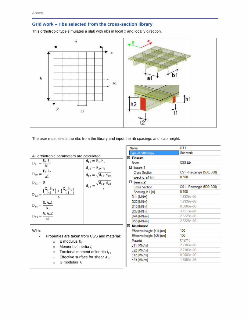
Annex

73

Grid work – ribs selected from the cross-section li brary

This orthotropic type simulates a slab with ribs in local x and local y direction.

The user must select the ribs from the library and input the rib spacings and slab height. All orthotropic parameters are calculated:

D~~ � E~. I~b1 D// � E/. I/a1 D~/ � 0Dgg � CG~. It~b1 E � CG/. It/a1 E4 Dnn � G. Az1b1 D�� G. Az2a1

d~~ � E~. h~d// � E/. h/d~/ � �d~~. d//dgg � �d~~. d//2

With: • Properties are taken from CSS and material:

o E modulus ,� o Moment of inertia +� o Torsional moment of inertia +�� o Effective surface for shear B�� o G modulus G�


74

References

[1] De Roeck, G.: De eindige-elementenmethode, Leuven, 1991. [2] Kolar, vl. et al.: FEM Principles and practice of the Finite Element Method (Czech language), Computer press, 1997.

Topic Training Finite Element Method

Documents

Transcript of Topic Training Finite Element Method