TOPIC T1: MASS, MOMENTUM AND ENERGY AUTUMN 2013 … · Hydrostatics is the study of fluids at rest....

Hydraulics 2 T1-1 David Apsley

TOPIC T1: MASS, MOMENTUM AND ENERGY AUTUMN 2013

Objectives

(1) Extend continuity and momentum principles to non-uniform velocity.

(2) Apply continuity and Bernoulli’s equation to flow measurement and tank-emptying.

(3) Learn methods for dealing with non-ideal flow.

Contents

0. Basics

0.1 Notation

0.2 Dimensionless groups

0.3 Definitions

0.4 Principles of fluid mechanics

0.5 Physical constants

0.6 Properties of common fluids

1. Continuity (conservation of mass)

1.1 Mass and volume fluxes

1.2 Conservation of mass

1.3 Flows with non-uniform velocity

2. Forces and momentum

2.1 Control-volume formulation of the momentum principle

2.2 Fluid forces

2.3 Boundary layers and flow separation

2.4 Drag and lift coefficients

2.5 Calculation of momentum flux

2.6 The wake-traverse method for measurement of drag

3. Energy

3.1 Bernoulli’s equation

3.2 Fluid head

3.3 Static and stagnation pressure

3.4 Flow measurement

3.5 Tank filling and emptying

3.6 Summary of methods for incorporating non-ideal flow

References Hamill (2011) – Chapters 1, 2, 4, 5, 7

Chadwick and Morfett (2013) – Chapters 1, 2, 3

Massey (2011) – Chapters 1, 2, 3, 4

White (2011) – Chapters 1, 2, 3


0. BASICS 0.1 Notation

x (x, y, z) position; (z is usually vertical)

t time

u (u, v, w) velocity; (V is often used for the average speed in a pipe or channel)

p pressure

p – patm is the gauge pressure;

p* = p + ρgz is the piezometric pressure

T temperature

Fluid properties:

ρ density (mass per unit volume)

γ ρg specific weight (weight per unit volume)

s.g. ρ/ρref specific gravity (or relative density);

“ref” = water (for liquids) or air (for gases)

μ dynamic viscosity (stress per unit velocity gradient)

ν μ/ρ kinematic viscosity

σ surface tension (force per unit length)

K bulk modulus (pressure change divided by fractional change in volume)

k conductivity of heat (heat flux per unit area per unit temperature gradient)

c speed of sound

0.2 Dimensionless Groups

νμ

ρRe

ULUL Reynolds

1 number (viscous flow)

gL

UFr Froude

2 number (open-channel hydraulics)

c

UMa Mach

3 number (compressible flow)

σ

ρWe

2 LU Weber

4 number (surface tension)

U and L are representative length and velocity scales. You should always state which ones

you are using for a particular flow (e.g. average velocity and diameter for pipe flow).

Topic T3 (Dimensional Analysis) will introduce other important dimensionless groups.

1 Osborne Reynolds (1842-1912); appointed first Professor of Engineering at Owens College (later to become

the University of Manchester); his apparatus is on display in the basement of the George Begg building. 2 William Froude (1810-1879), British naval architect; developed scaling laws for the model testing of ships.

3 Ernst Mach (1838-1916), Austrian physicist and philosopher.

4 Moritz Weber (1871-1951), developed modern dimensional analysis; actually named the Re and Fr numbers.


0.3 Definitions

A fluid is a substance that flows; i.e. continues to deform under a shear stress.

A solid will deform initially but then reach static equilibrium under such a stress.

Fluids may be liquids (definite volume; free surface) or gases (expand to fill any container).

Hydrostatics is the study of fluids at rest.

Hydrodynamics is the study of fluids in motion.

Hydraulics is the study of the flow of liquids (usually water).

Aerodynamics is the study of the flow of gases (usually air).

All fluids are compressible to some degree, but their flow can be approximated as

incompressible (i.e. pressure changes due to motion don’t cause significant density changes)

for velocities much less than the speed of sound ( 1480 m s–1

in water, 340 m s–1

in air).

An ideal fluid is one with no viscosity. It doesn’t exist, but it can be a good approximation.

A Newtonian fluid is one for which viscous stress is proportional to velocity gradient:

y

u

d

dμτ

μ is the viscosity. Most fluids of interest (including air and water) are Newtonian, but there

are some important non-Newtonian ones (e.g. mud, blood, paint, polymer solutions).

Real flows may be laminar (adjacent layers slide smoothly over each other) or turbulent

(subject to random fluctuations about a mean flow). If the viscosity is too small to maintain a

smooth, orderly flow, then a laminar flow undergoes transition and becomes turbulent.

Although transition to turbulence is dependent on a number of factors, including surface

roughness, the primary determinant is the Reynolds number

νμ

ρRe

ULUL (1)

U and L are typical velocity and length scales of the flow. In general:

“high” Re ↔ turbulent

“low” Re ↔ laminar

Typical critical Reynolds numbers for transition between laminar and turbulent flow are:

pipe flow: ReD 2300 (based on diameter and average velocity)

circular cylinder: ReD 3105 (based on diameter and approach velocity)

flat plate: Rex 5105 – 310

6 (based on distance and free-stream velocity)

Important: The Reynolds number and its critical value depend on the particular flow and on

which velocity and length scale are chosen to define it: see the different values above. The

particular choices should, therefore, be stated. (For example, you could choose to use either

radius or diameter as the length scale for flow in a pipe, and they would give a factor-of-2

difference in Reynolds number even though the flow is the same.) Why are the values quoted

for circular cylinder and flat plate above so much larger than that for pipe flow?

The majority of civil-engineering flows are fully turbulent.


0.4 Principles of Fluid Mechanics

Hydrostatics

In stationary fluid, pressure forces balance weight. Hence, pressure increases with depth.

Hydrostatic Equation

zgp ΔρΔ or gz

pρ

d

d (2)

Pressure also varies in the same way with depth in a moving fluid if there is no vertical

component of acceleration or, as a good approximation, if the vertical acceleration << g.

For a constant-density fluid these can also be written

0)ρ(Δ gzp or constantgzp ρ

p + ρgz is called the piezometric pressure.

Thermodynamics

For compressible fluids thermodynamics and heat input are important and one requires, in

addition, an equation of state connecting pressure, density (or volume) and temperature; e.g.

Ideal Gas Law

p = ρRT (3)

p is the absolute pressure, whilst T is the absolute temperature in Kelvin:

15.273)C()K( TT (4)

The gas constant R is a constant for any particular gas and is given by R = R0 / m, where R0 is

the universal gas constant and m is the mass of one mole. For dry air, R = 287 J kg–1

K–1

. The

equation is a rearrangement of the form used in chemistry: TnRpV 0 , where V is volume

and n is the number of moles of gas.

Fluid Dynamics

Continuity (Mass Conservation) Mass is conserved.

For steady flow: (mass flux)in = (mass flux)out

Momentum Principle Force = rate of change of momentum.

For steady flow: force = (momentum flux)out – (momentum flux)in

Energy

Change in energy = heat supplied + work done

For incompressible flow: change of kinetic energy = work done


The Energy Equation

(i) Incompressible Flow

For incompressible flow the energy equation is a purely mechanical equation and can be

derived from the momentum principle.

Bernoulli’s Equation

Steady incompressible flow without losses:

eamlinelong a strconstant aUgzp 2

21 ρρ

More generally, in steady incompressible flow,

forcesveconservatinonbymassunitperdoneworkUgzp

)()ρ

(Δ 2

21 (5)

Δ( ) means “change in” and the RHS of (5) represents energy input to the flow by pumps or

removed from the flow by turbines or friction.

(ii) Compressible Flow

For compressible flow the energy equation involves thermodynamics. The energy per unit

mass is supplemented by the internal energy e and energy can also be transferred to the fluid

as heat. (5) is replaced by:

uiddone on flworkfluidtosuppliedheatUgzp

e )ρ

(Δ 2

21 (6)

The quantity ρ/pe is called enthalpy.

0.5 Physical Constants

Gravitational acceleration: g = 9.81 m s–2

(at British latitudes)

Universal gas constant: R0 = 8.314 J mol–1

K–1

Standard atmospheric pressure: 1 atmosphere = 1.01325105 Pa = 1.01325 bar

Standard temperature and pressure (s.t.p):

IUPAC (International Union of Pure and Applied Chemistry): 0° C (273.15 K) and 105 Pa.

ISO (International Standards Organisation): 0° C (273.15 K) and 1 atm (1.01325105 Pa).


0.6 Properties of Common Fluids Properties are given at 1 atmosphere and 20 ºC unless otherwise specified.

Air

Density: ρ = 1.20 kg m–3

(ρ = 1.29 kg m–3

at 0 ºC)

Specific weight: γ = 11.8 N m–3

Dynamic viscosity: μ = 1.8010–5

kg m–1

s–1

(or Pa s)

Kinematic viscosity: ν = 1.5010–5

m2 s

–1

Specific heat capacity at constant volume: cv = 718 J kg–1

K–1

Specific heat capacity at constant pressure: cp = 1005 J kg–1

K–1

Gas constant: R = 287 J kg–1

K–1

Speed of sound: c = 343 m s–1

Water

Density: ρ = 998 kg m–3

(ρ = 1000 kg m–3

at 0 ºC)

Specific weight: γ = 9790 N m–3

Dynamic viscosity: μ = 1.00310–3

kg m–1

s–1

(or Pa s)

Kinematic viscosity: ν = 1.00510–6

m2 s

–1

Surface tension: σ = 0.0728 N m–1

Speed of sound: c = 1482 m s–1

Mercury


Ethanol


Fluid properties – especially viscosity – change significantly with temperature.

Water Air

T (°C) ρ (kg m–3

) μ (Pa s) ν (m2 s

–1) ρ (kg m

–3) μ (Pa s) ν (m

2 s

–1)

0 1000 1.78810–3

1.78810–6 1.29 1.7110

–5 1.3310

–5

20 998 1.00310–3

1.00510–6

1.20 1.8010–5

1.5010–5

50 988 0.54810–3

0.55510–6

1.09 1.9510–5

1.7910–5

100 958 0.28310–3

0.29510–6

0.946 2.1710–5

2.3010–5

As temperature increases:

viscosities of liquids decrease;

viscosities of gases increase.

(Explain why.)

The viscosity of gases may be approximated by Sutherland’s law:

ST

ST

T

T 0

2/3

00μ

μ (7)

The constants differ between gases. For air: T0 = 273 K, μ0 = 1.7110–5

Pa s, S = 110.4 K.


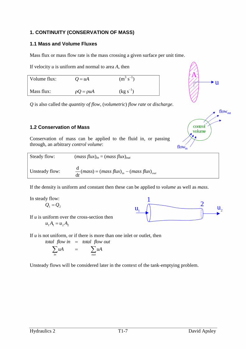
1. CONTINUITY (CONSERVATION OF MASS)

1.1 Mass and Volume Fluxes

Mass flux or mass flow rate is the mass crossing a given surface per unit time.

If velocity u is uniform and normal to area A, then

Volume flux: uAQ (m3 s

–1)

Mass flux: uAQ ρρ (kg s–1

)

Q is also called the quantity of flow, (volumetric) flow rate or discharge.

1.2 Conservation of Mass

Conservation of mass can be applied to the fluid in, or passing

through, an arbitrary control volume:

Steady flow: (mass flux)in = (mass flux)out

Unsteady flow: outin mass fluxmass fluxmasst

)()()(d

d

If the density is uniform and constant then these can be applied to volume as well as mass.

In steady flow:

21 QQ

If u is uniform over the cross-section then

2211 AuAu

If u is not uniform, or if there is more than one inlet or outlet, then

outin

uAuA

outflowtotalinflowtotal

Unsteady flows will be considered later in the context of the tank-emptying problem.

uA

controlvolume

flowin

flowout

u1

u2

12


Example. The figure shows a converging two-dimensional duct in which flow enters in two layers. A

fluid of specific gravity 0.8 flows as the top layer at a velocity of 2 m s–1

and water flows

along the bottom layer at a velocity of 4 m s–1

. The two layers are each of thickness 0.5 m.

The two flows mix thoroughly in the duct and the mixture exits to atmosphere with the

velocity uniform across the section of depth 0.5 m.

0.5 m

2 m/s

4 m/s

0.5 m

0.5 m

p =15 kN/m1

2

(a) Determine the velocity of flow of the mixture at the exit.

(b) Determine the density of the mixture at the exit.

(c) If the pressure p1 at the upstream section is 15 kPa, what is the force per unit width

exerted on the duct? (Do part (c) after Section 2 on the Momentum Principle).

Answer: (a) 6 m s–1

; (b) 933 kg m–3

; (c) 7.8 kN

1.3 Flows With Non-Uniform Velocity

The continuity principle may be extended to cases where u varies over a cross-section (e.g.

flow in pipes or flow in a boundary layer) by breaking the section down into infinitesimal

areas dA, across each of which the velocity is constant:

AuQ dd

The total quantity of flow is found by summation or, in the limit of small areas, integration:

Volume flow rate:

AuQ d (8)

The average velocity (or bulk velocity) is that constant velocity which would give the same

total flow rate; i.e. AuQ av or

Average velocity: area

rateflow

A

Quav (9)

To find the average velocity for a non-uniform velocity profile first find the flow rate Q.


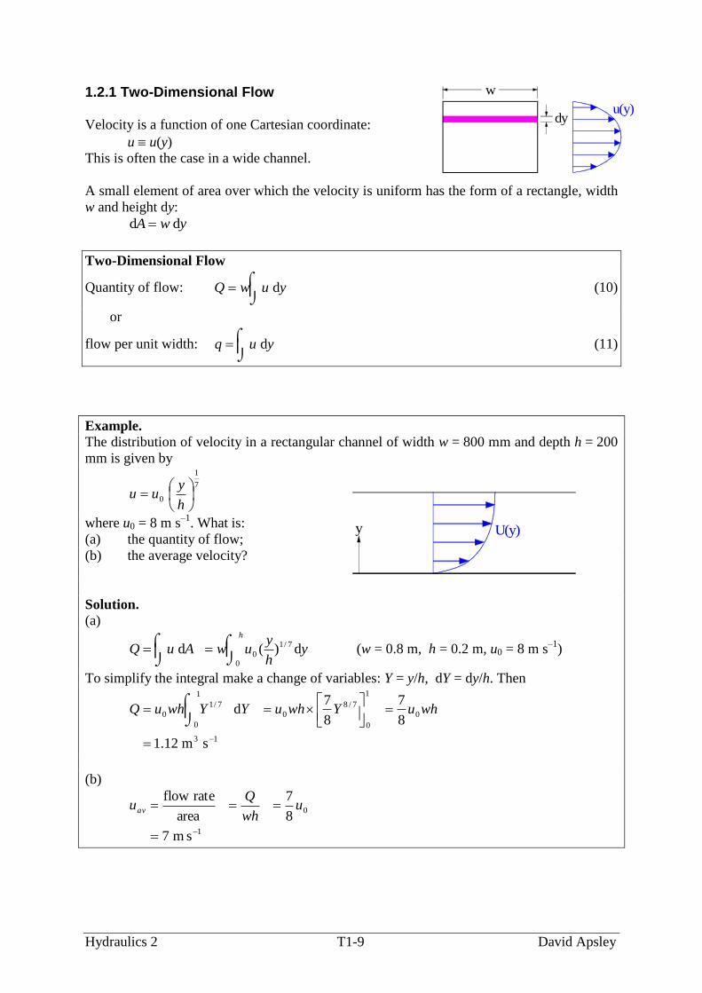
1.2.1 Two-Dimensional Flow

Velocity is a function of one Cartesian coordinate:

u u(y)

This is often the case in a wide channel.

A small element of area over which the velocity is uniform has the form of a rectangle, width

w and height dy:

ywA dd

Two-Dimensional Flow

Quantity of flow:

yuwQ d (10)

or

flow per unit width:

yuq d (11)

Example. The distribution of velocity in a rectangular channel of width w = 800 mm and depth h = 200

mm is given by

7

1

0

h

yuu

where u0 = 8 m s–1

. What is:

(a) the quantity of flow;

(b) the average velocity?

Solution. (a)

h

yh

yuwAuQ

0

7/1

0 d)(d (w = 0.8 m, h = 0.2 m, u0 = 8 m s–1

)

To simplify the integral make a change of variables: Y = y/h, dY = dy/h. Then

13

0

1

0

7/8

0

1

0

7/1

0

sm12.1

8

7

8

7d

whuYwhuYYwhuQ

(b)

1

0

s m7

8

7

area

rateflow

uwh

Quav

w

dyu(y)

y U(y)


1.2.2 Axisymmetric Flow

Velocity is a function of the radial coordinate r:

)(ruu

Examples include pipes and jets.

A small element of area over which the velocity is uniform is an infinitesimal hoop of radius

r and thickness dr:

rrA dπ2d (12)

Axisymmetric Flow

Quantity of flow:

rruQ dπ2 (13)

Example.

Fully-developed laminar flow in a pipe of radius R has velocity profile:

)/1( 22

0 Rruu

Find the average velocity in terms of u0.

Solution.

The average velocity can be found by dividing the flow rate by the area. For the flow rate:

RR

rrRrurruQ0

22

0

0

d)/1(π2dπ2

For convenience, make a change of variables: s = r/R, ds = dr/R . Then

0

2

1

0

42

0

2

1

0

3

0

2

1

0

2

0

2

π2

1

42π2d)(π2d)1(π2

uR

ssuRsssuRsssuRQ

Hence,

0

2

2

1

π

u

R

Quav

Note: For velocity profiles measured in an experiment (where the integral would be

evaluated graphically as the area under a curve), it is unnatural and inaccurate to have the

integrand (u 2πr) vanishing at the centre, r = 0, since this is where velocity is highest; in this

case (13) can be rewritten, making the change of variables s = r2, ds = 2r dr, as

suQ dπ or

2dπ ruQ (14)

i.e.

quantity of flow = π (area under a u vs r2 graph)

drr

u(r)


F

uout

uin

2. FORCES AND MOMENTUM

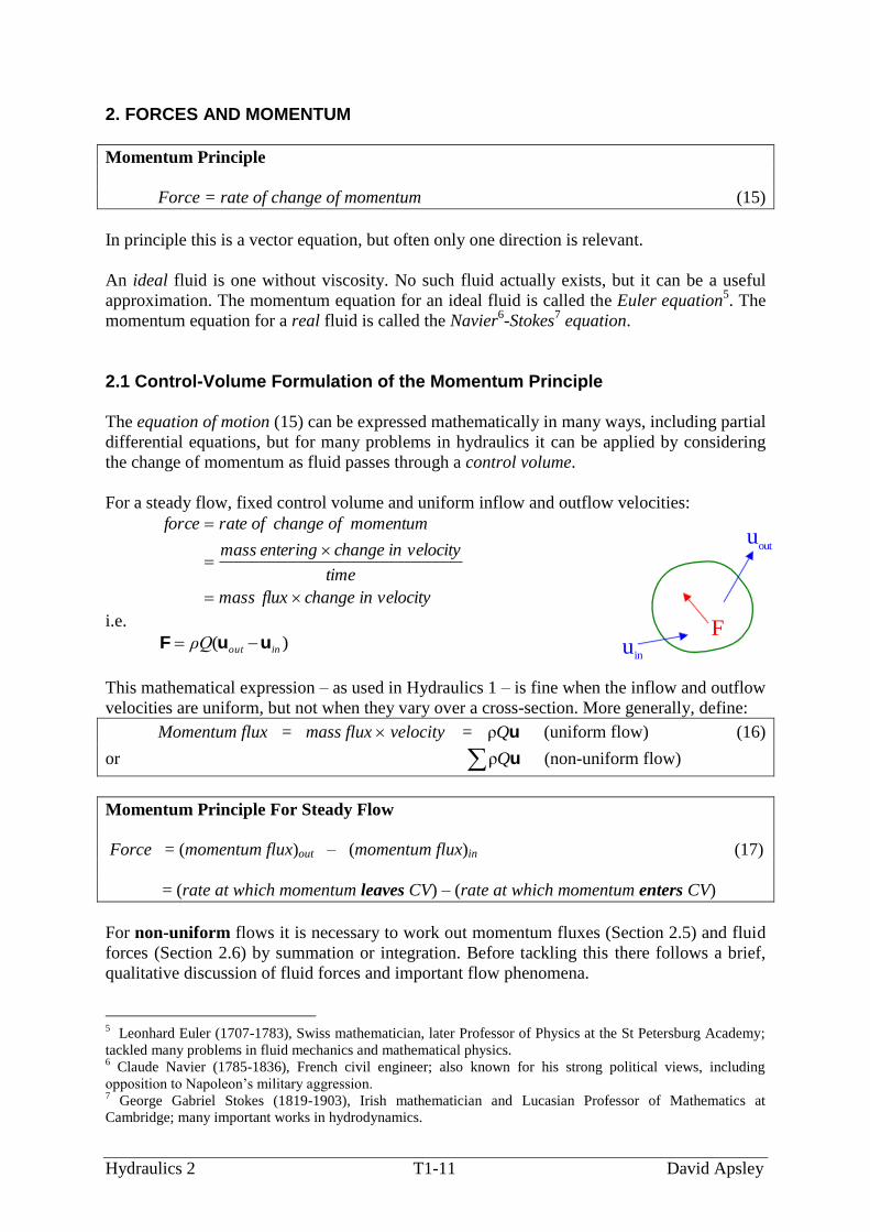
Momentum Principle

Force = rate of change of momentum (15)

In principle this is a vector equation, but often only one direction is relevant.

An ideal fluid is one without viscosity. No such fluid actually exists, but it can be a useful

approximation. The momentum equation for an ideal fluid is called the Euler equation5. The

momentum equation for a real fluid is called the Navier6-Stokes

7 equation.

2.1 Control-Volume Formulation of the Momentum Principle

The equation of motion (15) can be expressed mathematically in many ways, including partial

differential equations, but for many problems in hydraulics it can be applied by considering

the change of momentum as fluid passes through a control volume.

For a steady flow, fixed control volume and uniform inflow and outflow velocities:

velocityinchangefluxmass

time

velocitychange in enteringmass

momentumofchangeofrateforce

i.e.

)( inoutρQ uuF

This mathematical expression – as used in Hydraulics 1 – is fine when the inflow and outflow

velocities are uniform, but not when they vary over a cross-section. More generally, define:

Momentum flux = mass flux velocity = uQρ (uniform flow) (16)

or uQρ (non-uniform flow)

Momentum Principle For Steady Flow

Force = (momentum flux)out – (momentum flux)in (17)

= (rate at which momentum leaves CV) – (rate at which momentum enters CV)

For non-uniform flows it is necessary to work out momentum fluxes (Section 2.5) and fluid

forces (Section 2.6) by summation or integration. Before tackling this there follows a brief,

qualitative discussion of fluid forces and important flow phenomena.

5 Leonhard Euler (1707-1783), Swiss mathematician, later Professor of Physics at the St Petersburg Academy;

tackled many problems in fluid mechanics and mathematical physics. 6 Claude Navier (1785-1836), French civil engineer; also known for his strong political views, including

opposition to Napoleon’s military aggression. 7 George Gabriel Stokes (1819-1903), Irish mathematician and Lucasian Professor of Mathematics at

Cambridge; many important works in hydrodynamics.


2.2 Fluid Forces

The total force on the fluid in a control volume is a combination of:

body forces (proportional to volume); e.g.

– weight;

– centrifugal and Coriolis forces8 (apparent forces in rotating frames);

surface forces (exerted by adjacent fluid and proportional to area); e.g.

– pressure forces;

– viscous forces;

reactions from solid boundaries.

Weight acts whether the fluid is moving or not and would be balanced by a hydrostatic

pressure distribution. It can be excluded from the analysis if we consider only departures

from the hydrostatic state and work with the piezometric pressure.

Since surface forces are proportional to area they are usually expressed in terms of stresses:

area

forcestress or areastressforce (18)

Pressure (p) is a normal stress directed inward to a surface. For

the control volume shown the net pressure force in the x

direction from pressures on the left (L) and right (R) faces is

App RL )(

Since the net force only involves the difference in pressures it does not matter whether

absolute, gauge or other relative pressure is used, as long as one is consistent.

Shear stresses (τ) act tangentially to surfaces. For the control

volume shown the net force in the x direction from shear stresses on

the top (T) and bottom (B) faces is

AA BT ττ

(What is denoted τ here is strictly τxy; in complex flows other components such as τxx, τyz, …

may be important. By convention, τxy is the force per unit area in the x direction that the fluid

on the upper (greater y) side of the interface exerts on the fluid on the lower (smaller y) side.)

Laminar and Turbulent Flow

Shear stresses arise from two sources: viscous forces and, in turbulent flow,

the net transfer of momentum across an interface by turbulent fluctuations

which, as far as the mean flow is concerned, has the same effect as a force.

For Newtonian fluids, viscous stress is proportional to velocity gradient. If

velocity u is a function of y only then, in laminar flow:

y

u

d

dμτ (19)

8Very important in environmental flows: winds and ocean currents; also arise in rotating machinery, e.g. pumps.

Ap A

Rp A

L

A T

B

A

A

yu(y)


This defines the dynamic viscosity, μ. (In complex flow a more general stress-strain

relationship is required, but this is beyond the scope of this course.)

In turbulent flow one is usually interested in the time-averaged mean velocity u . Since

momentum transfer between fast- and slow-moving fluid is dominated by turbulent mixing

rather than viscous stresses the mean shear stress is substantially greater than yu/ddμ .

2.3 Boundary Layers and Flow Separation

The ideal-fluid (zero-viscosity) approximation is inapplicable if

viscous effects have a major effect on the flow. The most important

example of the latter is boundary-layer separation.

In real fluids velocity vanishes at solid boundaries (the no-slip

condition). There is a boundary layer where velocity changes rapidly

from its value in the free stream to zero at the boundary. At high

Reynolds numbers boundary layers are usually very thin.

In an adverse pressure gradient (where pressure increases and velocity decreases in the

direction of flow; for example, in an expanding channel) the net force in the opposite

direction to flow may cause the more-slowly-moving fluid near the boundary to reverse

direction. This backflow leads to flow separation.

adverse pressure

gradient

backflow

flowseparation

speeds up ... ... slows down

For bodies with sharp corners flow separation occurs at all but the smallest Reynolds

numbers and causes a large increase in pressure (or form) drag

because the pressures upstream and downstream are very

different. (Upstream pressure is high because flow is brought

to rest; downstream pressure is low because velocities in the

recirculating flow are small, so that the pressure is almost

constant and equal to that at the separation point.)

For more gently curved bodies separation may or may not occur.

Turbulence prevents or delays flow separation because it facilitates the transport of fast-

moving fluid from the free stream into the near-wall region, maintaining forward motion.

Thus, counter-intuitively, provoking a boundary layer on a curved surface into turbulence

(e.g. by roughening the surface) may actually reduce drag because it delays or prevents

separation. This is why golf balls have dimples.

Free stream

Boundary layer

H L

Highpressure

Lowpressure


2.4 Drag and Lift Coefficients

The force on a body in a flow can be resolved into components.

U0

lift F

drag

Drag = component of force parallel to the approach flow.

Lift = component of force perpendicular to the approach flow.

The relative importance of drag or lift forces is quantified by non-dimensionalising them by

dynamic pressure ( 2

021 ρU ) area:

Drag and Lift Coefficients

AU

dragcD 2

021 ρ

, AU

liftcL 2

021 ρ

(20)

U0 is a representative velocity scale and is usually taken as the approach-flow velocity. A is a

representative area which depends on the body geometry and the nature of the flow (see

below). Just like the Reynolds number, both should be specified when defining cD or cL.

Drag on Bluff or Streamlined Bodies

Bluff bodies (i.e. flow separation)

force is predominantly pressure drag

A is the projected area (normal to the flow)

cD is of order 1

Streamlined bodies (i.e. no flow separation)

force is predominantly viscous drag

A is the plan area (parallel to the flow)

cD << 1

AU0

AU0


2.5 Calculation of Momentum Flux

The momentum principle for steady flow may be written for a general control volume:

inout luxmomentum fluxmomentum f Force )()(

For uniform velocity:

u

u

)ρ(

)ρ(

uA

Q

velocityfluxmassfluxmomentum

(21)

For 1-d flow in the x direction,

Auluxmomentum f 2ρ (22)

If the velocity is not uniform then subdivide into small areas over which the velocity is

uniform and then sum or integrate:

Auluxmomentum f dρ 2 (23)

Special Cases

Velocity profile Momentum flux

(i) Uniform

Area A

AU 2ρ

(ii) 2-dimensional

dA = w dy

w

dyu(y)

yuw dρ 2

(iii) Axisymmetric

dA = 2πr dr

drr

u(r)

drru π2ρ 2


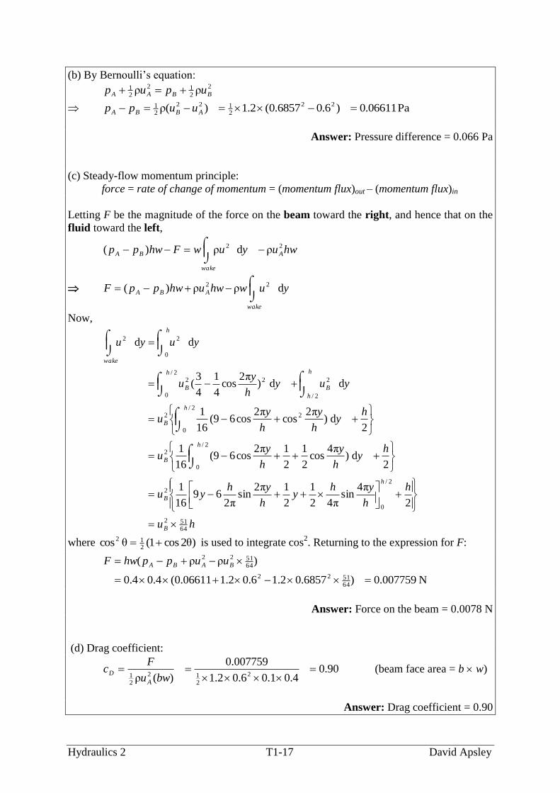
Example. A two-dimensional beam of height b = 100 mm spans a square air-conditioning duct of height

h = 400 mm (see the figure below). The approach flow is uniform (uA = 0.6 m s–1

), whilst the

downstream velocity profile is 2-dimensional and given by:

2/if,

2/if,)π2

cos4

1

4

3(

hyu

hyh

yu

u

B

B

The pressure is uniform over the height of the duct at both sections. Neglecting drag on the

walls of the duct find:

(a) the value of uB;

(b) the difference between pressures at upstream and downstream sections, assuming that

Bernoulli’s equation holds outside the wake region;

(c) the force on the beam.

Also,

(d) define a suitable drag coefficient for the beam and calculate its value.

Take the density of air as 1.2 kg m–3

.

0.6 m/s400 mm

100 mm

Solution.

(a) Let w be the width of the tunnel. (In this particular case, w = h because the duct is square.)

By continuity (i.e., the same volumetric flow rate at both sections):

h

h

B

h

B

wake

A

yuyh

yuw

ywuhwu

2/

2/

0

dd)π2

cos4

1

4

3(

d

Hence, dividing by width w (equivalent to working per unit width):

hu

hhu

hh

yhyuhu

B

B

h

BA

87

21

83

21

2/

0

)(

π2sin

π24

1

4

3

Thus,

1s m 6857.06.07

8

7

8 AB uu

Answer: u2 = 0.69 m s–1


(b) By Bernoulli’s equation:

2

212

21 ρρ BBAA upup

Pa 06611.0)6.06857.0(2.1)(ρ 22

2122

21 ABBA uupp

Answer: Pressure difference = 0.066 Pa

(c) Steady-flow momentum principle:

force = rate of change of momentum = (momentum flux)out – (momentum flux)in

Letting F be the magnitude of the force on the beam toward the right, and hence that on the

fluid toward the left,

hwuyuwFhwpp A

wake

BA

22 ρdρ)(

wake

ABA yuwhwuhwppF dρρ)( 22

Now,

hu

h

h

yhy

h

yhyu

hy

h

y

h

yu

hy

h

y

h

yu

yuyh

yu

yuyu

B

h

B

h

B

h

B

h

h

B

h

B

h

wake

64512

2/

0

2

2/

0

2

2/

0

22

2/

22/

0

22

0

22

2

π4sin

π42

1

2

1π2sin

π269

16

1

2d)

π4cos

2

1

2

1π2cos69(

16

1

2d)

π2cos

π2cos69(

16

1

dd)π2

cos4

1

4

3(

dd

where )θ2cos1(θcos212 is used to integrate cos

2. Returning to the expression for F:

N 007759.0)6857.02.16.02.106611.0(4.04.0

)ρρ(

645122

645122

BABA uupphwF

Answer: Force on the beam = 0.0078 N

(d) Drag coefficient:

90.04.01.06.02.1

007759.0

)(ρ 2

212

21

bwu

Fc

A

D (beam face area = b w)

Answer: Drag coefficient = 0.90


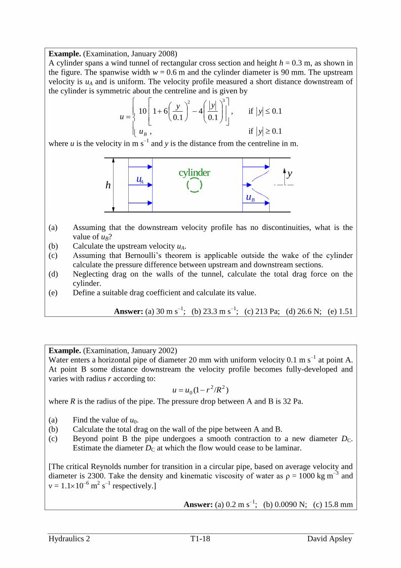
Example. (Examination, January 2008)

A cylinder spans a wind tunnel of rectangular cross section and height h = 0.3 m, as shown in

the figure. The spanwise width w = 0.6 m and the cylinder diameter is 90 mm. The upstream

velocity is uA and is uniform. The velocity profile measured a short distance downstream of

the cylinder is symmetric about the centreline and is given by

1.0if,

1.0if,1.0

41.0

6110

32

yu

yyy

u

B

where u is the velocity in m s–1

and y is the distance from the centreline in m.

y

h

cylinderuA

uB

(a) Assuming that the downstream velocity profile has no discontinuities, what is the

value of uB?

(b) Calculate the upstream velocity uA.

(c) Assuming that Bernoulli’s theorem is applicable outside the wake of the cylinder

calculate the pressure difference between upstream and downstream sections.

(d) Neglecting drag on the walls of the tunnel, calculate the total drag force on the

cylinder.

(e) Define a suitable drag coefficient and calculate its value.

Answer: (a) 30 m s–1

; (b) 23.3 m s–1

; (c) 213 Pa; (d) 26.6 N; (e) 1.51

Example. (Examination, January 2002)

Water enters a horizontal pipe of diameter 20 mm with uniform velocity 0.1 m s–1

at point A.

At point B some distance downstream the velocity profile becomes fully-developed and

varies with radius r according to:

)/1( 220 Rruu

where R is the radius of the pipe. The pressure drop between A and B is 32 Pa.

(a) Find the value of u0.

(b) Calculate the total drag on the wall of the pipe between A and B.

(c) Beyond point B the pipe undergoes a smooth contraction to a new diameter DC.

Estimate the diameter DC at which the flow would cease to be laminar.

[The critical Reynolds number for transition in a circular pipe, based on average velocity and

diameter is 2300. Take the density and kinematic viscosity of water as ρ = 1000 kg m–3

and

ν = 1.110–6

m2 s

–1 respectively.]

Answer: (a) 0.2 m s–1

; (b) 0.0090 N; (c) 15.8 mm


2.6 The Wake-Traverse Method for Measurement of Drag Objects in a flow experience a force. If

the fluid exerts a force F on the body then

the body exerts a reaction force of the

same magnitude but opposite direction on

the fluid. By measuring the change in

momentum and pressure one can use the

momentum principle to deduce the force on the body.

Suitable control volumes for constrained (e.g. wind tunnel) and unconstrained flow are shown

below. In both cases upper and lower boundaries are streamlines, across which there is no

flow. Fluid passing close to the body forms a wake of low velocity downstream.

If the flow is constrained by boundaries (e.g.

in a wind tunnel) then the velocity outside the

wake must increase slightly (in order to pass

the same volume flow rate through the same

area), with a compensating fall in pressure.

This is called a blockage effect.

In the unconstrained case, upper and lower

boundaries should be sufficiently far away

that pressure is equal to that in the free

stream. (Otherwise the pressure force on the

curved boundaries will have a net component

in the x direction.)

The steady-state momentum principle gives:

force on fluid = (momentum flux)out – (momentum flux)in

inoutoutin

AuAuApApF dρdρdd 22 (24)

The two integrals on the RHS tend to be individually much larger than F, but almost cancel

each other out. For experimentally-determined velocity profiles this cancellation means that a

small error in either will lead to a huge error in F. To avoid this, it is common to rewrite the

RHS as a single integral over the wake. Provided that the inflow velocity is uniform (uin):

out

in

out

in

fluxmass

in

inin

in

AuuAuuAuuAu dρdρdρdρ 2

Substituting in (24) and rearranging gives

out

inin AppuuuF d)]()(ρ[ (25)

(Sometimes this is used as the starting point for the momentum principle, since ρu dA(uin – u)

is the rate of change of momentum in an individual stream tube carrying mass flux ρu dA.

However, this is only useful if the inflow velocity is uniform.)

FForce on BODY

F

Force on FLUID

inflow wake

body

inflow wake

streamline

body


For unconstrained flows, pressures upstream and downstream are equal (pin – p = 0), as are

the free-stream velocities (uin = u∞,out). In the constrained case, it can be shown that, provided

the wake is narrow compared with the duct height (so that the difference in free-stream

velocities is small), any pressure difference approximately compensates for the change in the

free-stream velocity9. Thus, in the case of either unconstrained flow or low blockage ratio,

(25) can be satisfactorily approximated by

out

AuuuF d)(ρ (26)

where u∞ denotes the free-stream velocity at outflow. Thus, hydrodynamic forces may be

deduced indirectly by measuring the velocity profile in the wake, rather than directly using a

force balance. This is called the wake traverse method and you will have an opportunity to

use it in the wind-tunnel laboratory experiment.

9 By Bernoulli, )(ρ 22

,21

inoutoutin uupp ; the error in (26) can then, after a lot of algebra, be shown to

be

Auu outin d)(ρ 2

,21 , which is second order in the (small) free-stream velocity difference.


3. ENERGY

3.1 Bernoulli’s Equation10

Mechanical-energy principle:

change in kinetic energy = work done

In rate form, with work done by conservative forces (here, gravity) rewritten in terms of

potential energy:

forcesveconservatinonofworkingrate of

energypotentialkineticofchangeofrate

)(

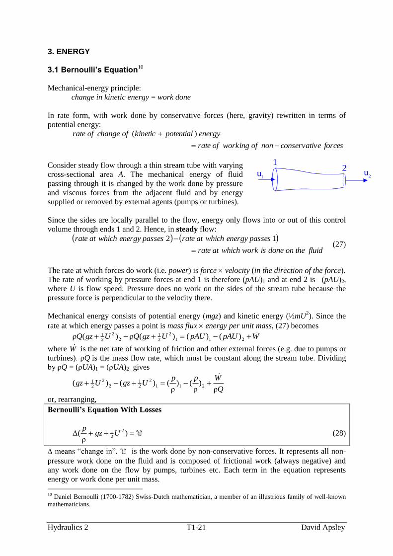
Consider steady flow through a thin stream tube with varying

cross-sectional area A. The mechanical energy of fluid

passing through it is changed by the work done by pressure

and viscous forces from the adjacent fluid and by energy

supplied or removed by external agents (pumps or turbines).

Since the sides are locally parallel to the flow, energy only flows into or out of this control

volume through ends 1 and 2. Hence, in steady flow:

fluid theondoneiswhich workrate at

ses energy paswhichrate atses energy paswhichrate at

12 (27)

The rate at which forces do work (i.e. power) is force velocity (in the direction of the force).

The rate of working by pressure forces at end 1 is therefore (pAU)1 and at end 2 is –(pAU)2,

where U is flow speed. Pressure does no work on the sides of the stream tube because the

pressure force is perpendicular to the velocity there.

Mechanical energy consists of potential energy (mgz) and kinetic energy (½mU2). Since the

rate at which energy passes a point is mass flux energy per unit mass, (27) becomes

WpAUpAUUgzQUgzQ 211

2

21

2

2

21 )()()(ρ)(ρ

where W is the net rate of working of friction and other external forces (e.g. due to pumps or

turbines). ρQ is the mass flow rate, which must be constant along the stream tube. Dividing

by ρQ = (ρUA)1 = (ρUA)2 gives

Q

WppUgzUgz

ρ)

ρ()

ρ()()( 211

2

21

2

2

21

or, rearranging,

Bernoulli’s Equation With Losses

W )ρ

(Δ 2

21 Ugz

p (28)

means “change in”. W is the work done by non-conservative forces. It represents all non-

pressure work done on the fluid and is composed of frictional work (always negative) and

any work done on the flow by pumps, turbines etc. Each term in the equation represents

energy or work done per unit mass.

10

Daniel Bernoulli (1700-1782) Swiss-Dutch mathematician, a member of an illustrious family of well-known

mathematicians.

u1

u2

12


Thermal or Compressible Flow

(28) can be extended to thermal flows (boilers, condensers, refrigerators, ...) or compressible

flow by using the total energy equation:

change in (internal + kinetic) energy = work done + heat input

(28) then becomes

heatsupplyingofrateworkdoingofrateUgzp

e )ρ

(Δ 2

21 (29)

The RHS is energy input per unit mass. The quantity ρ

pe is called the specific enthalpy.

Incompressible Flow

If there are no losses and no work done by pumps or turbines then (28) reduces to

2

21

ρUgz

pconstant (along a streamline) (30)

For incompressible flow, density ρ is also constant along a streamline. Then we have:

Bernoulli’s equation (without losses):

2

21 ρρ Ugzp constant (along a streamline) (31)

where

p = static pressure

p + ρgz = piezometric pressure

2

21 ρU = dynamic pressure

Note the assumptions:

along a streamline (different streamlines may have a different “constant”)

steady

incompressible

inviscid (no losses)


3.2 Fluid Head

In hydraulics both energy and pressure are often expressed in length units; e.g. “metres of

water” or “millimetres of mercury”. In equation (31) each term has dimensions of pressure, or

of energy per unit volume. Dividing by weight per unit volume (i.e. specific weight) ρg, these

become energies per unit weight. This has dimensions of length and is called fluid head.

headtotal

g

Uz

g

p

pressuretotalUgzp

or ,weightunitperenergy2ρ

or ,volumeunitperenergyρρ2

2

21

(32)

g

p

ρ = pressure head

zg

p

ρ = piezometric head

g

U

2

2

= dynamic head

Energy losses due to friction and the change in pressure imparted by pumps are often

specified in terms of head. For pumps the rate of working (i.e. power) is given by

gQHpower ρ (33)

where Q is the quantity of flow and H is the change in head. This will be revisited in Topic 4.

3.3 Static and Stagnation Pressure

A stagnation point is a point on a streamline

where the velocity is reduced to zero. In

general, any non-rotating solid obstacle in a

stream produces a stagnation point next to its

upstream surface, where the flow streamlines

must split to pass around the obstacle.

The stagnation pressure (or Pitot pressure)

p0 is that pressure which would arise if the

flow were brought instantaneously to rest. By

Bernoulli’s equation it is given (for

incompressible fluids) by 2

21 ρUp . Define:

stagnation pressure 2

21 ρUp

static pressure p

dynamic pressure 2

21 ρU

The dynamic pressure (and hence the flow velocity) is found by measuring the difference

between stagnation and static pressures.

stagnation point(highest pressure)U = 0, P = P0

2

21

0 Uρpp


3.4 Flow Measurement

3.4.1 Measurement of Pressure – Manometry Principles

Basic rules of hydrostatics for a connected body of fluid:

(1) Same fluid, same height same pressure

(2) Same fluid, different height zgp ΔρΔ

(3) Different fluids: pressure is continuous at an interface

U-Tube Manometer

By (1) the pressure at level C is the same in both arms of the

manometer. By (2) and (3) it can be found from pA and pB

respectively by summing the changes in pressure over the heights

of columns of fluid:

armright

mBC

armleft

A ghgyppyhgp ρρ)(ρ

where ρ and ρm are the densities of the working fluid and the

manometer fluid respectively. Cancelling ρgy and subtracting ρgh

gives the pressure difference BA ppp Δ :

Manometer Equation

ghp m )ρρ(Δ (34)

If the working fluid is a gas then ρ « ρm and (34) can be approximated by

ghp mρΔ (35)

Inclined Manometer

Differences in head may be small and difficult to

measure accurately. The movement of the

manometer fluid may be amplified by inclining

the manometer. It is the vertical difference in

height which is proportional to pressure

differences: this is given in terms of the much

larger length L by

θsinLh (36)

A B

h

C

y

m

L (large)

h (small)


3.4.2 Measurement of Velocity

Method: bring the fluid to rest at one point and measure the difference between static and

stagnation (Pitot) pressures:

pressuredynamic

pressurestatic

pressurePitot

Upp 2

21

0 ρ

Examples.

(1) Open-channel flow.

The free-surface streamline and the streamline

approaching the Pitot tube both have the same

total head, but where the flow is brought to rest at

the front of the Pitot tube the dynamic head U2/2g

is converted into pressure head and subsequently

elevation.

(2) Pipe flow – Pitot tube and piezometer

Same principle as above, but the pressure in the

pipe is usually higher than atmospheric, so that

water rises in the piezometer also.

(3) Pitot-static tube – measures both

stagnation and static pressures in the

same instrument.

free surfaceU /2g

2

stagnation point

U

piezometer Pitot tube

Ug2

2

static holes

stagnation point

static pressure tube

total pressure tube


3.4.3 Measurement of Quantity of Flow

General Method

Provide a locally reduced area to change speed, and measure the resulting change in pressure.

The combination of continuity and Bernouilli’s equation yields bulk velocity and flow rate.

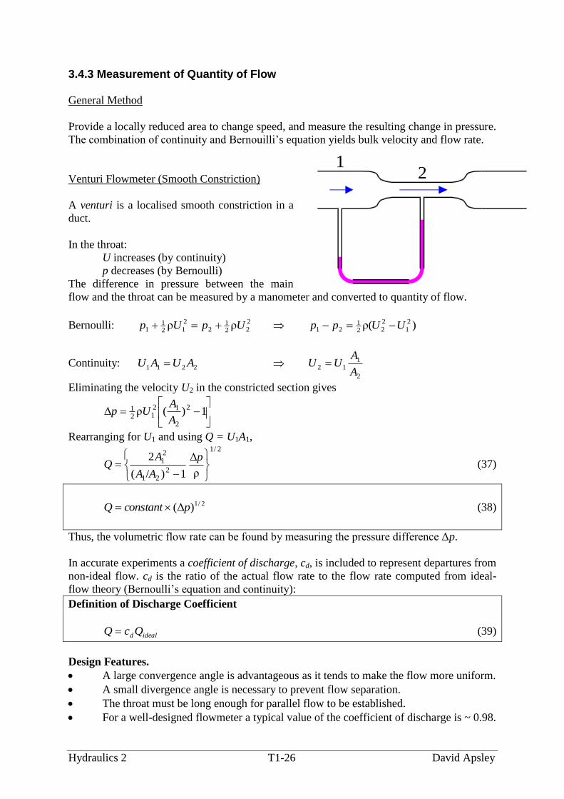
Venturi Flowmeter (Smooth Constriction)

A venturi is a localised smooth constriction in a

duct.

In the throat:

U increases (by continuity)

p decreases (by Bernoulli)

The difference in pressure between the main

flow and the throat can be measured by a manometer and converted to quantity of flow.

Bernoulli: 2

221

2

2

121

1 ρρ UpUp )(ρ 2

1

2

221

21 UUpp

Continuity: 2211 AUAU 2

112

A

AUU

Eliminating the velocity U2 in the constricted section gives

1)(ρΔ 2

2

1212

1

A

AUp

Rearranging for U1 and using Q = U1A1,

2/1

221

21

ρ

Δ

1)/(

2

p

AA

AQ (37)

2/1)Δ( pconstantQ (38)

Thus, the volumetric flow rate can be found by measuring the pressure difference Δp.

In accurate experiments a coefficient of discharge, cd, is included to represent departures from

non-ideal flow. cd is the ratio of the actual flow rate to the flow rate computed from ideal-

flow theory (Bernoulli’s equation and continuity):

Definition of Discharge Coefficient

idealdQcQ (39)

Design Features.

A large convergence angle is advantageous as it tends to make the flow more uniform.

A small divergence angle is necessary to prevent flow separation.

The throat must be long enough for parallel flow to be established.

For a well-designed flowmeter a typical value of the coefficient of discharge is ~ 0.98.

12


Orifice Flowmeter (Abrupt Constriction)

An orifice is an aperture of small streamwise thickness through which

fluid passes.

The streamwise thickness determines frictional losses.

The fluid cannot turn immediately, so the emerging stream tube

continues to narrow as far as the vena contracta – the section of

minimum cross-sectional area.

An orifice meter is a means of measuring the

flow rate in a duct by measuring the differential

pressure across an orifice.

It is basically an extreme variant of the venturi

meter with the divergent region omitted. The

basic premise is that the pressure throughout the

recirculating eddy is essentially equal to that at

the vena contracta.

Advantages: cheap and small.

Disadvantage: considerable loss of energy.

By the same process as that for the venturi meter one obtains:

2/1

21

21

ρ

Δ

1)/(

2

p

AA

AQ

v

where Av is the area of the vena contracta (not the aperture). Av is not obvious from the

geometry. If Av is replaced by the area of the orifice then this may be compensated for by a

coefficient of discharge, but, in practice, theory is simply used to deduce the form of the

relationship between the flow rate Q and the pressure drop Δp:

2/1)Δ( pconstantQ (40)

with the constant determined by calibration.

vena contracta


3.5 Tank Filling and Emptying

3.5.1 Free Discharge Under Gravity

For a tank, discharging as a free jet, with free surface at a

distance h above the discharging fluid, apply Bernoulli’s

equation between the free surface and the jet:

2

2

221

21

2

121

1 ρρρρ gzUpgzUp

Here, hzzUppp atm 21121 ,0, , so that:

ghzzgU ρ)(ρρ 21

2

221

This amounts to an exchange of gravitational potential energy

for kinetic energy and gives

Torricelli’s Formula11

ghU exit 2 (41)

Ideally the discharge would be

)orifice of area(2 ghQideal (42)

This is not true in practice because of

frictional effects (small for a sharp-edged orifice)

contraction (area of vena contracta < area of orifice).

If these are significant then a coefficient of discharge cd may be introduced to compensate for

both of these effects:

idealdQcQ

cd must be measured experimentally. For a sharp-edged orifice, cd 0.6 – 0.65. Contraction

effects can be reduced by using a bellmouth (i.e. curved) exit to minimise rapid changes in

direction. However, frictional losses are then greater.

Strictly, Bernoulli’s formula is invalid in the reservoir/orifice problem if the free-surface

level changes rapidly (since it is then time-dependent). If, however, the tank cross section is

much larger than that of the orifice, then a quasi-steady approximation is OK. Also, if the

aperture is large (compared with the height to the free surface), then the value of Uexit will be

different for each streamline passing through the orifice (because each will have a different

value of h). The total discharge would then have to be found by integration.

11

Evangelista Torricelli (1608-1647); Italian mathematician of barometer fame; served as secretary to Galileo.

h

1

2


3.5.2 Continuity Equation

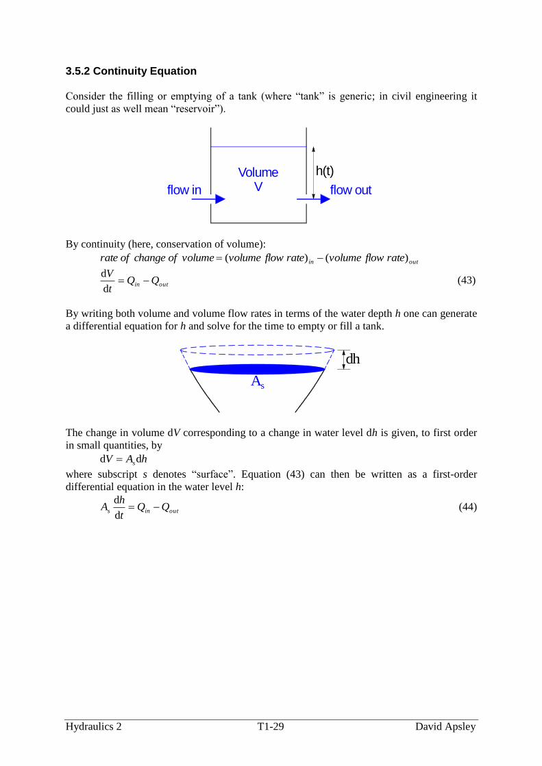
Consider the filling or emptying of a tank (where “tank” is generic; in civil engineering it

could just as well mean “reservoir”).

VolumeV

h(t)

flow in flow out

By continuity (here, conservation of volume):

outin rateflowvolumerateflowvolumevolumeofchangeofrate )()(

outin QQt

V

d

d (43)

By writing both volume and volume flow rates in terms of the water depth h one can generate

a differential equation for h and solve for the time to empty or fill a tank.

As

dh

The change in volume dV corresponding to a change in water level dh is given, to first order

in small quantities, by

hAV sdd

where subscript s denotes “surface”. Equation (43) can then be written as a first-order

differential equation in the water level h:

outins QQt

hA

d

d (44)


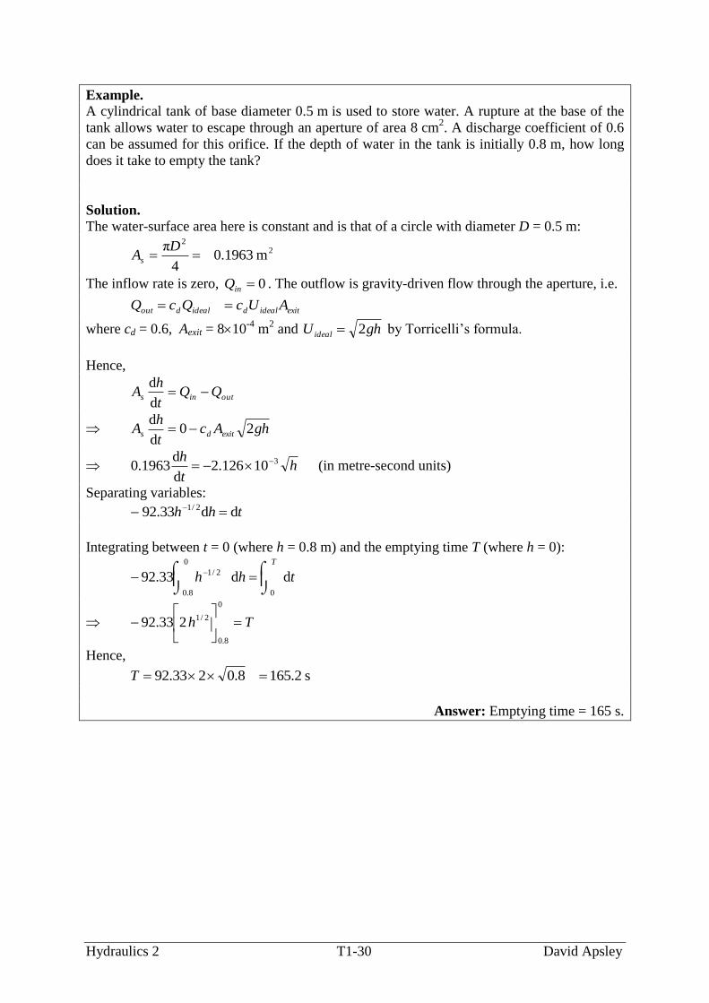
Example.

A cylindrical tank of base diameter 0.5 m is used to store water. A rupture at the base of the

tank allows water to escape through an aperture of area 8 cm2. A discharge coefficient of 0.6

can be assumed for this orifice. If the depth of water in the tank is initially 0.8 m, how long

does it take to empty the tank?

Solution.

The water-surface area here is constant and is that of a circle with diameter D = 0.5 m:

22

m1963.04

π

DAs

The inflow rate is zero, 0inQ . The outflow is gravity-driven flow through the aperture, i.e.

exitidealdidealdout AUcQcQ

where cd = 0.6, Aexit = 810-4

m2 and ghU ideal 2 by Torricelli’s formula.

Hence,

outins QQt

hA

d

d

ghAct

hA exitds 20

d

d

ht

h 310126.2d

d1963.0 (in metre-second units)

Separating variables:

thh dd33.92 2/1

Integrating between t = 0 (where h = 0.8 m) and the emptying time T (where h = 0):

T

thh0

0

8.0

2/1 dd33.92

Th

0

8.0

2/1233.92

Hence,

s2.1658.0233.92 T

Answer: Emptying time = 165 s.


In general the water-surface area As is also a function of water depth h.

Example.

A conical hopper of semi-vertex angle 30º contains water to a depth of 0.8 m. If a small hole

of diameter 20 mm is suddenly opened at its point, estimate (assuming a discharge coefficient

cd = 0.8):

(a) the initial discharge (quantity of flow);

(b) the time taken to reduce the depth of water to 0.4 m.

0.8 m30

o

Answer: (a) 0.996 L s–1

; 177 s.


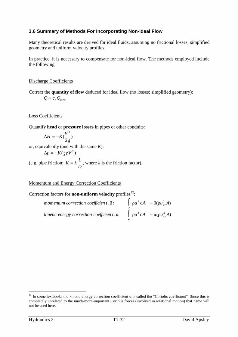
3.6 Summary of Methods For Incorporating Non-Ideal Flow

Many theoretical results are derived for ideal fluids, assuming no frictional losses, simplified

geometry and uniform velocity profiles.

In practice, it is necessary to compensate for non-ideal flow. The methods employed include

the following.

Discharge Coefficients

Correct the quantity of flow deduced for ideal flow (no losses; simplified geometry):

ideald QcQ

Loss Coefficients

Quantify head or pressure losses in pipes or other conduits:

)2

(Δ2

g

VKH

or, equivalently (and with the same K):

)ρ(Δ 2

21 VKp

(e.g. pipe friction: D

LK λ , where λ is the friction factor).

Momentum and Energy Correction Coefficients

Correction factors for non-uniform velocity profiles12

:

)ρ(αdρ:α,

)ρ(βdρ:β,

33

22

AuAutcoefficiencorrectionenergykinetic

AuAutcoefficiencorrectionmomentum

av

av

12 In some textbooks the kinetic-energy correction coefficient α is called the “Coriolis coefficient”. Since this is

completely unrelated to the much-more-important Coriolis forces (involved in rotational motion) that name will

not be used here.

TOPIC T1: MASS, MOMENTUM AND ENERGY AUTUMN 2013 … · Hydrostatics is the study of fluids at rest....

Documents

Transcript of TOPIC T1: MASS, MOMENTUM AND ENERGY AUTUMN 2013 … · Hydrostatics is the study of fluids at rest....