Topic modeling for OLAP on multidimensional text databases: topic cube and its applications

Topic Modeling for OLAP on Multidimensional Text Databases: Topic Cubeand its Applications

Duo Zhang1∗, ChengXiang Zhai1, Jiawei Han1, Ashok Srivastava2 and Nikunj Oza2

1 Department of Computer Science, University of Illinois at Urbana-Champaign,Urbana, Illinois, USA

2 Intelligent Systems Division, NASA Ames Research Center, Moffett Field, California, USA

Received 5 May 2009; revised 7 September 2009; accepted 18 September 2009DOI:10.1002/sam.10059

Published online 20 November 2009 in Wiley InterScience (www.interscience.wiley.com).

Abstract: As the amount of textual information grows explosively in various kinds of business systems, it becomes more andmore desirable to analyze both structured data records and unstructured text data simultaneously. Although online analyticalprocessing (OLAP) techniques have been proven very useful for analyzing and mining structured data, they face challengesin handling text data. On the other hand, probabilistic topic models are among the most effective approaches to latent topicanalysis and mining on text data. In this paper, we study a new data model called topic cube to combine OLAP with probabilistictopic modeling and enable OLAP on the dimension of text data in a multidimensional text database. Topic cube extends thetraditional data cube to cope with a topic hierarchy and stores probabilistic content measures of text documents learned througha probabilistic topic model. To materialize topic cubes efficiently, we propose two heuristic aggregations to speed up the iterativeExpectation-Maximization (EM) algorithm for estimating topic models by leveraging the models learned on component datacells to choose a good starting point for iteration. Experimental results show that these heuristic aggregations are much fasterthan the baseline method of computing each topic cube from scratch. We also discuss some potential uses of topic cube andshow sample experimental results. 2009 Wiley Periodicals, Inc. Statistical Analysis and Data Mining 2: 378–395, 2009

Keywords: topic cube; text OLAP; multidimensional text database

1. INTRODUCTION

Data warehouses are widely used in today’s businessmarket for organizing and analyzing large amounts of data.An important technology to exploit data warehouses isthe online analytical processing (OLAP) technology [1–3],which enables flexible interactive analysis of multidimen-sional data in different granularities. It has been widelyapplied to many different domains [4–6]. OLAP on datawarehouses is mainly supported through data cubes [7,8].

As unstructured text data grows quickly, it is more andmore important to go beyond the traditional OLAP on struc-tured data to also tap into the huge amounts of text dataavailable to us for data analysis and knowledge discovery.These kinds of text data often exist either in the characterfields of data records or in a separate place with links tothe data records through joinable common attributes. Thus,conceptually we have both structured data and unstruc-tured text data in a database. For convenience, we willrefer to such a database as a multidimensional text database

Correspondence to: Duo Zhang ([email protected])

(MTD), to distinguish it from both the traditional relationaldatabases and the text databases which consist primarily oftext documents.

As argued convincingly in Ref. [9], simultaneous analysisof both structured data and unstructured text data is requiredin order to fully take advantage of all the knowledge in allthe data, and will mutually enhance each other in terms ofknowledge discovery, thus bringing more values to busi-ness. Unfortunately, traditional data cubes, though capableof dealing with structured data, would face challenges foranalyzing unstructured text data.

As a specific example, consider Aviation Safety Report-ing System (ASRS) [10], which is the world’s largest repos-itory of safety information provided by aviation’s frontlinepersonnel. The database has both structured data (e.g., time,airport, and light condition) and text data such as narrativesabout anomalous events written by pilots or flight attendantsas illustrated in Table 1. A text narrative usually containshundreds of words.

This repository contains valuable information about avi-ation safety and is a main resource for analyzing causes of

2009 Wiley Periodicals, Inc.

Zhang et al.: Topic Modeling for Text OLAP 379

Table 1. An example of multidimensional text database inASRS.

ACN Time Airport · · · Light Narrative

101285 1999 01 MSP · · · Daylight Document 1101286 1999 01 CKB · · · Night Document 2101291 1999 02 LAX · · · Dawn Document 3

recurring anomalous aviation events. Since causal factorsdo not explicitly exist in the structured data part of therepository, but are buried in many narrative text fields, it iscrucial to support an analyst to mine such data flexibly withboth OLAP and text content analysis in an integrative man-ner. Unfortunately, the current data cube and OLAP tech-niques can only provide limited support for such integrativeanalysis. In particular, although they can easily supportdrill-down and roll-up on structured attributes dimensionssuch as ‘time’ and ‘location’, they cannot support an analystto drill-down and roll-up on the text dimension accordingto some meaningful topic hierarchy defined for the anal-ysis task (i.e., anomalous event analysis), such as the oneillustrated in Fig. 1.

In the tree shown in Fig. 1, the root represents the aggre-gation of all the topics (each representing an anomalousevent). The second level contains some general anomalytypes defined in Ref. [11], such as ‘anomaly altitude devi-ation’ and ‘anomaly maintenance problem’. A child topicnode represents a specialized event type of the event typeof its parent node. For example, ‘undershoot’ and ‘over-shoot’ are two special anomalous events of ‘anomaly alti-tude deviation’.

Being able to drill-down and roll-up along such a hierar-chy would be extremely useful for causal factor analysis ofanomalous events. Unfortunately, with today’s OLAP tech-niques, the analyst cannot easily do this. Imagine that ananalyst is interested in analyzing altitude deviation prob-lems of flights in Los Angeles in 1999. With the tradi-tional data cube, the analyst can only pose a query suchas (Time=‘1999’, Location=‘LA’) and obtain a large setof text narratives, which would have to be further analyzedwith separate text mining tools.

Even if the data warehouse can support keyword querieson the text field, it still would not help the analyst that

much. Specifically, the analyst can now pose a more con-strained query (Time=‘1999’, Location=‘LA’, Keyword=‘altitude deviation’), which would give the analyst asmaller set of more relevant text narratives (i.e., thosematching the keywords ‘altitude deviation’) to work with.However, the analyst would still need to use a separate textmining tool to further analyze the text information to under-stand causes of this anomaly. Moreover, exact keywordmatching would also likely miss many relevant text narra-tives that are about deviation problems but do not contain ormatch the keywords ‘altitude’ and ‘deviation’ exactly; forexample, a more specific word such as ‘overshooting’ mayhave been used in a narrative about an altitude deviationproblem.

A more powerful OLAP system should ideally inte-grate text mining more tightly with the traditional cubeand OLAP, and allow the analyst to drill-down and roll-up on the text dimension along a specified topic hierarchyin exactly the same way as he/she could on the locationdimension. For example, it would be very helpful if the ana-lyst can use a similar query (Time=‘1999’, Location=‘LA’,Topic=‘altitude deviation’) to obtain all the relevant nar-ratives to this topic (including those that do not neces-sarily match exactly the words ‘altitude’ and ‘deviation’),and then drill-down into the lower-level categories such as‘overshooting’ and ‘undershooting’ according to the hier-archy (and roll-up again) to change the view of the contentof the text narrative data. Note that although the query hasa similar form to that with the keyword query mentionedabove, its intended semantics is different: ‘altitude devia-tion’ is a topic taken from the hierarchy specified by theanalyst, which is meant to match all the narratives coveringthis topic including those that may not match the keywords‘altitude’ and ‘deviation’.

Furthermore, the analyst would also need to digest thecontent of all the narratives in the cube cell correspond-ing to each topic category and compare the content acrossdifferent cells that correspond to interesting context vari-ations. For example, at the level of ‘altitude deviation’, itwould be desirable to provide a summary of the content ofall the narratives matching this topic, and when we drill-down to ‘overshooting’, it would also be desirable to allow

ALL

Anomaly Altitude Deviation …… Anomaly Maintenance Problem …… Anomaly Inflight Encounter

Undershoot Overshoot ImproperDocumentation

ImproperMaintenance

Birds Turbulence…… …………

Fig. 1 A hierarchical topic tree for anomalous events.

Statistical Analysis and Data Mining DOI:10.1002/sam

380 Statistical Analysis and Data Mining, Vol. 2 (2009)

the analyst to easily obtain a summary of the narrativescorresponding to the specific subcategory of ‘overshootingdeviation’. With such summaries, the analyst would be ableto, for example, compare the content of narratives about thedeviation problem across different locations in 1999. Sucha summary can be regarded as a content measure of the textin a cell.

This example illustrates that in order to integrate textanalysis seamlessly into OLAP, we need to support thefollowing functions:Topic dimension hierarchy: We need to map text docu-ments semantically to an arbitrary topic hierarchy specifiedby an analyst so that the analyst can drill-down and roll-up on the text dimension (i.e., adding text dimension toOLAP). Note that we do not always have training data (i.e.,documents with known topic labels) for learning. Thus, wemust be able to perform this mapping without training data.Text content measure: We need to summarize the contentof text documents in a data cell (i.e., computing contentmeasure on text). Since different applications may pre-fer different forms of summaries, we need to be able torepresent the content in a general way that can accommo-date many different ways to further customize a summaryaccording to the application needs.Efficient materialization: We need to materialize cubeswith text content measures efficiently.

Although there has been some previous work on textdatabase analysis [12,13] and integrating text analysis withOLAP [14,15], to the best of our knowledge, no previouswork has proposed a specific solution to extend OLAP tosupport all these functions mentioned above. The closestprevious work is the IBM work [9], where the authors pro-posed some high-level ideas for leveraging existing textmining algorithms to integrate text mining with OLAP.However, in their work, the cubes are still traditional datacubes, thus the integration is loose and text mining is innature external to OLAP. Moreover, the issue of material-izing cubes to efficiently handle text dimension has not beaddressed. We will review the related work in more detailin Section 2.

In this paper, we study a new data cube model calledtopic cube to support the two key functions of OLAP ontext dimension (i.e., topic dimension hierarchy and textcontent measure) with a unified probabilistic framework.Our basic idea is to leverage probabilistic topic modeling[16,17], which is a principled method for text mining, andcombine it with OLAP. Indeed, probabilistic latent seman-tic analysis (PLSA) and similar topic models have recentlybeen very successfully applied to a large range of text min-ing problems including hierarchical topic modeling [18,19],author-topic analysis [20], spatiotemporal text mining [21],sentiment analysis [22], and multistream bursty pattern find-ing [23]. They are among the most effective text mining

techniques. We proposed topic cube to combine them withOLAP to enable effective mining of both structured dataand unstructured text within a unified framework.

Specifically, we extend the traditional cube to incorpo-rate the PLSA model [16] so that a data cube would carryparameters of a probabilistic model that can indicate thetext content of cells. Our basic assumption is that we canuse a probability distribution over words to model a topicin text. For example, a distribution may assign high proba-bilities to words such as ‘encounter’, ‘turbulence’, ‘height’,‘air’, and it would intuitively capture the theme ‘encounter-ing turbulence’ in the aviation report domain. We assumeall the documents in a cell to be word samples drawn froma mixture of many such topic distributions, and can thusestimate these hidden topic models by fitting the mixturemodel to the documents. These word distributions of topicscan thus serve as content measures of text documents. Inorder to respect the topic hierarchy specified by the analystand enable drill-down and roll-up on the text dimension, wefurther structure such distribution-based content measuresbased on the topic hierarchy specified by an analyst byusing the concept hierarchy to impose a prior (preference)on the word distributions characterizing each topic, so thateach word distribution would correspond to precisely onetopic in the hierarchy. By this way, we will learn word dis-tributions characterizing each topic in the hierarchy. Oncewe have a distributional representation of each topic, wecan easily map any set of documents to the topic hierarchy.

Note that topic cube supports the first two functions in aquite general way. First, when mapping documents into atopic hierarchy, the model could work with just some key-word description of each topic but no training data. Ourexperimental results show that this is feasible. If we dohave training data available, the model can also easily useit to enrich our prior; indeed, if we have many training dataand impose an infinitely strong prior, we essentially performsupervised text categorization with a generative model. Sec-ond, a multinomial word distribution serves well as a con-tent measure. Such a model (often called unigram languagemodel) has been shown to outperform the traditional vectorspace models in information retrieval [24,25], and can befurther exploited to generate more informative summariesif required. For example, in Ref. [26], such a unigramlanguage model has been successfully used to generate asentence-based impact summary of scientific literature. Ingeneral, we may further use these word distributions to gen-erate informative phrases [27] or comparative summariesfor comparing content across different contexts [22]. Thus,topic cube has potentially many interesting applications.

Computing and materializing such a topic cube in abrute force way is time-consuming. So to better sup-port the third function, we propose a heuristic algorithmto leverage estimated models for ‘component cells’ to



speed up the estimation of the model for a combinedcell. Estimation of parameters is done with an iterativeExpectation-Maximization (EM) algorithm. Its efficiencyhighly depends on where to start in the parameter space.Our idea for speeding it up can be described as follows:we would start with the smallest cells to be materialized,and use PLSA to mine all the topics in the hierarchicaltopic tree level by level from these cells. We then workon larger cells by leveraging the estimated parameters forthe small cells as a more efficient starting point. We callthis step as aggregation along the standard dimensions. Inaddition, when we mine the topics in the hierarchial treefrom cells, we can also leverage the estimated parametersfor topics in the lower levels to estimate the parametersfor topics in the higher levels. We call this step as aggre-gation along the topic dimension. Our experimental resultsshow that the proposed strategy, including both these twokinds of aggregations, can indeed speed up the estimationalgorithm significantly.

2. RELATED WORK

To the best of our knowledge, no previous work has uni-fied topic modeling with OLAP. However, some previousstudies have attempted to analyze text data in a relationaldatabase and support OLAP for text analysis. These stud-ies can be grouped into four categories, depending on howthey treat the text data.Text as fact: In this kind of approaches, the text data isregarded as a fact of the data records. When a user queriesthe database, the fact of the text data, e.g., term frequency,will be returned. BlogScope [28], which is an analysis andvisualization tool for blogosphere, belongs to this category.One feature of BlogScope is to depict the trend of a key-word. This is done by counting relevant blog posts in eachtime slot according to the input keyword and then draw-ing a curve of counts along the time axis. However, thisapproach cannot support OLAP operations such as drill-down and roll-up on the text dimension, which the proposedtopic cube would support.Text as character field: A major representative work in thisgroup is Ref. [29], where the text data is treated as a char-acter field. Given a keyword query, the records which havethe most relevant text in the field will be returned as results.For example, the following query (Location=‘Columbus’,keyword=‘LCD’) will fetch those records with locationequal to ‘Columbus’ and text field containing ‘LCD’. Thisessentially extends the query capability of a relationaldatabase to support search over a text field. However,this approach cannot support OLAP on the text dimensioneither.Text as categorical data: In this category, two similarworks to ours are BIW [9] and Polyanalyst [30]. Both of

them use classification methods to classify documents intocategories and attach documents with class labels. Suchcategory labels would allow a user to drill-down or roll-up along the category dimension, thus achieving OLAP ontext. However, in Ref. [9], only some high-level functiondescriptions are given with no algorithms given to effi-ciently support such OLAP operations on text dimension.Moreover, in both works, the notion of cube is still the tra-ditional data cube. Our topic cube differs from these twosystems in that we integrate text mining (specifically topicmodeling) more tightly with OLAP by extending the tra-ditional data cube to cover topic dimension and supporttext content measures, which leads to a new cube model(i.e., topic cube). Besides, we also propose heuristic meth-ods for materializing the new topic cube efficiently. Thetopic model provides a principled way to map arbitrarytext documents into topics specified in any topic hierarchydetermined by an application without requiring any trainingdata. Previous work would mostly either need documentswith known labels (for learning) which do not always exist,or cluster text documents in an unsupervised way, whichdoes not necessarily produce meaningful clusters to ananalyst, reducing the usefulness for performing OLAP onMTDs.Text as component of OLAP Using OLAP technologyto explore unstructured text data in a MTD has become apopular topic these years. In Ref. [31], the authors proposeda combination of keyword search and OLAP technique inorder to efficiently explore the content of a MTD. The basicidea is to use OLAP technology to explore the search resultsfrom a keyword query, where some dynamic dimensionsare constructed by extracting frequent and relevant phrasesfrom the text data. In Ref. [32], a model called text cube isproposed, in which IR measures of terms are used to sum-marize the text data in a cell. In Ref. [33], we proposeda new model called topic cube. The difference between atopic cube and previous work is in that a topic cube has atopic dimension which allows users to effectively explorethe unstructured text data from different semantic topics.Compared with frequent phrases or terms, such semantictopics are more meaningful to users. Furthermore, roll-upor drill-down along the topic dimension will also showusers different granularities of topics. In this paper, weextend [33] by discussing and analyzing some new mate-rialization strategies as well as new applications of topiccube.

Topic models have been extensively studied in recentyears [16–23,27,34], all showing that they are very usefulfor analyzing latent topics in text and discovering topicalpatterns. However, all the work in this line only dealswith pure text data. Our work can be regarded as a novelapplication of such models to support OLAP on MTDs.



3. TOPIC CUBE AS AN EXTENSIONOF DATA CUBE

The basic idea of topic cube is to extend the standard datacube by adding a topic hierarchy and probabilistic contentmeasures of text so that we can perform OLAP on thetext dimension in the same way as we perform OLAP onstructured data. In order to understand this idea, it is nec-essary to understand some basic concepts about data cubeand OLAP. So before we introduce topic cube in detail, wegive a brief introduction to these concepts.

3.1. Standard Data Cube and OLAP

A data cube is a multidimensional data model. It has threecomponents as input: a base table, dimensional hierarchies,and measures. A base table is a relational table in adatabase. A dimensional hierarchy gives a tree structureof values in a column field of the base table so that wecan define aggregation in a meaningful way. A measure isa fact of the data.

Roll-up and drill-down are two typical operations inOLAP. Roll-up would ‘climb up’ on a dimensional hier-archy to merge cells, whereas drill-down does the oppositeand split cells. Other OLAP operations include slice, dice,pivot, etc.

Two kinds of OLAP queries are supported in a data cube:point query and subcube query. A point query seeks a cellby specifying the values of some dimensions, whereas asubcube query would return a set of cells satisfying thequery.

3.2. Overview of Topic Cube

A topic cube is constructed based on a MTD, which wedefine as a multidimensional database with text fields. Anexample of such a database is shown in Table 1. We maydistinguish a text dimension from a standard (i.e., non-text)dimension in a MTD.

Another component used to construct a topic cube is ahierarchical topic tree. A hierarchical topic tree defines aset of hierarchically organized topics that users are mostlyinterested in, which are presumably also what we want tomine from the text. A sample hierarchical topic tree isshown in Fig. 1. In a hierarchical topic tree, each noderepresents a topic, and its child nodes represent the sub-topics under this super topic. Formally, the topics are placedin several levels L1, L2, . . . , Lm. Each level contains ki

topics, i.e., Li = (T1, . . . , Tki).

Given a MTD and a hierarchical topic tree, the mainidea of a topic cube is to use the hierarchical topic tree asthe hierarchy for the text dimension so that a user can drill-down and roll-up along this hierarchy to explore the content

of the text documents in the database. In order to achievethis, we would need to (i) map all the text documents totopics specified in the tree and (ii) compute a measure ofthe content of the text documents falling into each cell.

As will be explained in detail later, we can solve bothproblems simultaneously with a probabilistic topic modelcalled PLSA [16]. Specifically, given any set of text doc-uments, we can fit the PLSA model to these documents toobtain a set of latent topics in text, each represented by aword distribution (also called a unigram language model).These word distributions can serve as the basis of the ‘con-tent measure’ of text.

Since a basic assumption we make is that the analystwould be most interested in viewing the text data fromthe perspective of the specified hierarchical topic tree, wewould also like these word distributions corresponding wellto the topics defined in the tree. Note that an analyst willbe potentially interested in multiple levels of granularity oftopics, thus we also would like our content measure to have‘multiple resolutions’, corresponding to the multiple levelsof topics in the tree. Formally, for each level Li , if the treehas defined ki topics, we would like the PLSA to computeprecisely ki word distributions, each characterizing one ofthese ki topics. We will denote these word distributions asθj , for j = 1, . . . , ki , and p(w|θj ) is the probability ofword w according to distribution θj . Intuitively, the distri-bution θj reflects the content of the text documents when‘viewed’ from the perspective of the j th topic at level Li .

We achieve this goal of aligning a topic to a worddistribution in PLSA by using keyword descriptions of thetopics in the tree to define a prior on the word distributionparameters in PLSA so that all these parameters will bebiased toward capturing the topics in the tree. We estimatePLSA for each level of topics separately so as to obtain amultiresolution view of the content.

This established correspondence between a topic and aword distribution in PLSA has another immediate benefit,which is to help us map the text documents into topics in thetree because the word distribution for each topic can serveas a model for the documents that cover the topic. Actually,after estimating parameters in PLSA we also obtain anotherset of parameters that indicate to what extent each documentcovers each topic. It is denoted as p(θj |d), which means theprobability that document d covers topic θj . Thus, we caneasily predict which topic is the dominant topic in the setof documents by aggregating the coverage of a topic overall the documents in the set. That is, with p(θj |d), we canalso compute the topic distribution in a cell of documentsC as p(θj |C) = 1/|C|∑d∈C p(θj |d) (we assume p(d) areequal for all d ∈ C). Although θj is the primary contentmeasure which we will store in each cell, we will also storep(θj |d) as an auxiliary measure to support other ways ofaggregating and summarizing text content.



Time_key

Location_key

Environment_key

Topic_key{wi:p(wi|topic)}

{dj:p(topic|dj)}

Time_keyDayMonthYear

Location_keyCityStateCountry

Time

Location

Environment_keyLight

Environment

Measures

Topic_keyLower level topicHigher level topic

Topic

Fact table

Fig. 2 Star schema of a topic cube.

Thus essentially, our idea is to define a topic cube as anextension of a standard data cube by adding (i) a hierarchi-cal topic tree as a topic dimension for the text field and (ii)a set of probabilistic distributions as the content measureof text documents in the hierarchical topic dimension. Wenow give a systematic definition of the topic cube.

3.3. Definition of Topic Cube

DEFINITION 1: A topic cube is constructed based ona MTD D and a hierarchical topic tree H . It not only hasdimensions directly defined in the standard dimensions inthe database D but it also has a topic dimension which iscorresponding to the hierarchical topic tree. Drill-down androll-up along this topic dimension will allow users to viewthe data from different granularities of topics. The primarymeasure stored in a cell of a topic cube consists of a worddistribution characterizing the content of text documentsconstrained by values on both the topic dimension and thestandard dimensions (contexts).

The star schema of a topic cube for the ASRS example isgiven in Fig. 2. The dimension table for the topic dimensionis built based on the hierarchical topic tree. Two kindsof measures are stored in a topic cube cell, namely word

distribution of a topic p(wi |topic) and topic coverage bydocuments p(topic|dj ).

Figure 3 shows an example of a topic cube which is builtbased on ASRS data. The ‘Time’ and ‘Location’ dimensionsare defined in the standard dimensions in the ASRS textdatabase, and the topic dimension is added from the hierar-chical tree shown in Fig. 1. For example, the left cuboid inFig. 3 shows us word distributions of some finer topics like‘overshoot’ at ‘LAX’ in ‘Jan. 99’, whereas the right cuboidshows us word distributions of some coarse topics like‘Deviation’ at ‘LA’ in ‘1999’. Figure 4 shows two examplecells of a topic cube (with only word distribution measure)constructed from ASRS. The meaning of the first record isthat the top words of aircraft equipment problem occurredin flights during January 1999 are engine 0.104, pressure0.029, oil 0.023, checklist 0.022, hydraulic 0.020, . . . . Sowhen an expert gets the result from the topic cube, she willsoon know what are the main problems of equipments dur-ing January 1999, which shows the power of a topic cube.

3.3.1. Query

A topic cube supports the following query: (a1, a2, . . . ,

am, t). Here, ai represents the value of the ith dimensionand t represents the value of the topic dimension. Both ai

and t could be a specific value, a character ‘?’, or a charac-ter ‘*’. For example, in Fig. 3, a query (Location = ‘LAX’,Time = ‘Jan. 99’, t = ‘turbulence’) will return the worddistribution of topic ‘turbulence’ at ‘LAX’ in ‘Jan. 99’,whereas a query (Location = ‘LAX’, Time = ‘Jan. 99’,t = ‘?’) will return the word distribution of all the topics at

Time Anomaly Event Word Distribution

1999.01 equipmentengine 0.104, pressure 0.029, oil 0.023,

checklist 0.022, hydraulic 0.020, ...

1999.01ground

encounterstug 0.059, park 0.031, pushback 0.031, ramp0.029, brake 0.027, taxi 0.026, tow 0.023, ...

Fig. 4 Example cells in a topic cube.

TopicTopic TopicTopic

turbulenceturbulence

birdsbirds

undershootundershoot

overshootovershoot

LAX SJC MIA AUSJan.99

Jan.98Feb.99

1998

1999TXFLCA

Feb.98

Tim

e

Tim

e

Location Locationdrill-down roll-up

Encounter

Deviation

Fig. 3 An example of a topic cube.



‘LAX’ in ‘Jan. 99’. If t is specified as a ‘*’, e.g. (Location=‘LAX’, Time = ‘Jan. 99’, t = ‘*’), a topic cube will onlyreturn all the documents belong to cell (Location = ‘LAX’)and (Time = ‘Jan. 99’).

3.3.2. Operations

A topic cube not only allows users to carry out traditionalOLAP operations on the standard dimensions, but alsoallows users to do the same kinds of operations on the topicdimension. The roll-up and drill-down operations alongthe topic dimension will allow users to view the data indifferent levels (granularities) of topics in the hierarchicaltopic tree. Roll-up corresponds to change the view from alower level to a higher level in the tree, and drill-down isthe opposite. For example, in Fig. 3, an operation:

Roll-up on Anomaly Event (from Level 2 to Level 1)

will change the view of topic cube from finer topicslike ‘turbulence’ and ‘overshoot’ to coarser topics like‘Encounter’ and ‘Deviation’. The operation:

Drill-down on Anomaly Event (from Level 1 to Level 2)

just does the opposite change.

4. CONSTRUCTION OF TOPIC CUBE

To construct a topic cube, we first construct a generaldata cube (we call it GDC from now on) based on the stan-dard dimensions in the MTD D. In each cell of this cube,it stores a set of documents aggregated from the text field.Then, from the set of documents in each cell, we mine worddistributions of topics defined in the hierarchical topic treelevel by level. Next, we split each cell into K = ∑m

i=1 ki

cells. Here, ki is the number of topics in level i. Each ofthese new cells corresponds to one topic and stores its worddistribution (primary measure) and the topic coverage prob-abilities (auxiliary measure). At last, a topic dimension isadded to the data cube which allows users to view the databy selecting topics.

For example, to obtain a topic cube shown in Fig. 3,we first construct a data cube which has only two dimen-sions ‘Time’ and ‘Location’. Each cell in this data cubestores a set of documents. For example, in cell (‘LAX’,‘Jan. 99’), it stores the documents belonging to all therecords in the database where the ‘Location’ field is ‘LAX’and the ‘Time’ field is ‘Jan. 99’. Then, for the second levelof the hierarchical topic tree in Fig. 1, we mine topics, suchas ‘turbulence’, ‘bird’, ‘overshoot’, and ‘undershoot’, fromthe document set. For the first level of the hierarchical topictree, we mine topics such as ‘Encounter’ and ‘Deviation’from the document set. Next, we split the original cell, say

(‘LAX’, ‘Jan. 99’), into K cells, e.g. (‘LAX’, ‘Jan. 99’,‘turbulence’), (‘LAX’, ‘Jan. 99’, ‘Deviation’), etc. Here, K

is the total number of topics defined in the hierarchical topictree. At last, we add a topic dimension to the original datacube, and a topic cube is constructed.

Since a major component in our algorithm for construct-ing topic cube is the estimation of the PLSA model, we firstgive a brief introduction to this model before discussing theexact algorithm for constructing topic cube in detail.

4.1. Probabilistic Latent Semantic Analysis

Probabilistic topic models are generative models of textwith latent variables representing topics (more preciselysub-topics) buried in text. When using a topic model fortext mining, we generally would fit a model to the textdata to be analyzed and estimate all the parameters. Theseparameters would usually include a set of word distributionscorresponding to latent topics, thus allowing us to discoverand characterize hidden topics in text.

Most topic models proposed so far are based on tworepresentative basic models: PLSA [16] and latent Dirichletallocation (LDA) [17]. Although in principle both PLSAand LDA can be incorporated into OLAP with our ideas,we have chosen PLSA because its estimation can be donemuch more efficiently than for LDA. Below we give a briefintroduction to PLSA.

4.1.1. Basic PLSA

The basic PLSA [16] is a finite mixture model withk multinomial component models. Each word in a docu-ment is assumed to be a sample from this mixture model.Formally, suppose we use θi to denote a multinomial distri-bution capturing the ith topic, and p(w|θi) is the probabilityof word w given by θi . Let � = {θ1, θ2, . . . , θk} be theset of all k topics. The log likelihood of a collection oftext C is:

L(C|�) ∝∑

d∈C

∑

w∈V

c(w, d) logk∑

j=1

p(θj |d)p(w|θj ) (1)

where V is the vocabulary set of all words, c(w, d) thecount of word w in document d, and � the parameter setcomposed of {p(θj |d), p(w|θj )}d,w,j .

Given a collection, we may estimate PLSA using themaximum likelihood (ML) estimator by choosing the param-eters to maximize the likelihood function above. The MLestimator can be computed using the EM algorithm [35].The EM algorithm is a hill-climbing algorithm, and guar-anteed to find a local maximum of the likelihood function.It finds this solution through iteratively improving an initial



guess of parameter values using the following updating for-mulas (alternating between the E-step and M-step):

E-step:

p(zd,w = j) = p(n)(θj |d)p(n)(w|θj )∑kj ′=1 p(n)(θj ′ |d)p(n)(w|θj ′)

(2)

M-step:

p(n+1)(θj |d) =∑

w c(w, d)p(zd,w = j)∑j ′

∑w c(w, d)p(zd,w = j ′)

(3)

p(n+1)(w|θj ) =∑

d c(w, d)p(zd,w = j)∑w′

∑d c(w′, d)p(zd,w′ = j)

(4)

In the E-step, we compute the probability of a hiddenvariable zd,w, indicating which topic has been used togenerate the word w in d, which is calculated based onthe current generation of parameter values. In the M-step,we would use the information obtained from the E-step tore-estimate (i.e., update) our parameters. It can be shownthat the M-step always increases the value of the likelihoodfunction, meaning that the next generation of parametervalues would be better than the current one [35].

This updating process continues until the likelihood func-tion converges to a local maximum point which gives us theML estimate of the model parameters. Since the EM algo-rithm can only find a local maximum, its result is clearlyaffected by the choice of the initial values of parametersthat it starts with. If the starting point of parameter val-ues is already close to the maximum point, the algorithmwould converge quickly. As we will discuss in detail later,we will leverage this property to speed up the process ofmaterializing topic cube. Naturally, when a model has mul-tiple local maxima (as in the case of PLSA), we generallyneed to run the algorithm multiple times, each time witha different starting point, and finally use the one with thehighest likelihood.

4.1.2. PLSA aligned to a specified topic hierarchy

Directly applying PLSA model on a data set, we canextract k word distributions {p(w|θi)}i=1,. . .,k , characteriz-ing k topics. Intuitively, these distributions capture wordco-occurrences in the data, but the co-occurrence patternscaptured do not necessarily correspond to the topics in ourhierarchical topic tree. A key idea in our application ofPLSA to construct topic cube is to align the discoveredtopics with the topics specified in the tree through defininga prior with the topic tree and using Bayesian estimationinstead of the ML estimator which solely ‘listens’ to thedata.

Specifically, we could define a conjugate Dirichlet priorand use the maximum a posteriori (MAP) estimator to esti-mate the parameters [36]. We would first define a prior worddistribution p′(w|θj ) based on the keyword description ofthe corresponding topic in the tree; for example, we maydefine it based on the relative frequency of each keywordin the description. We assume that it is quite easy for ananalyst to give at least a few keywords to describe eachtopic. We then define a Dirichlet prior based on this distri-bution to essentially ‘force’ θj to assign a reasonably highprobability to words that have high probability according toour prior, i.e., the keywords used by the analyst to specifythis topic would all tend to have high probabilities accord-ing to θj , which further ‘steers’ the distribution to attractother words co-occurring with them, achieving the goal ofextracting the content about this topic from text.

4.2. Materialization

As discussed earlier, we use the PLSA model as ourtopic modeling method. To fully materialize a topic cube,we need to estimate PLSA and mine topics for eachcell in the original data cube. Suppose there are d stan-dard dimensions in the text database D, each dimen-sion has Li levels (i = 1, . . . , d), and each level hasn

(l)i values (i = 1, . . . , d; l = 1, . . . , Li). Then, we have

totally(∑L1

l=1 n(l)1

) × · · · × ( ∑Ld

l=1 n(l)d

)cells to mine if we

want to fully materialize a topic cube. One baseline strategyof materialization is an exhaustive method which computesthe topics cell by cell. However, this method is not efficientfor the following reasons:

(1) For each cell in GDC, the PLSA model uses EMalgorithm to calculate the parameters of topic models.This is an iterative method, and it may need hundredsof iterations before converge.

(2) For each cell in GDC, the PLSA model has the localmaximum problem. To avoid this problem and findthe global maximum, it needs to start from a numberof different random points to select the best one.

(3) The number of cells in GDC could be huge.

In general, measures in a data cube can be classifiedinto three categories based on the difficulty in aggregation:distributive, algebraic, and holistic [8]. The measure in atopic cube is the word distributions of topics obtained fromPLSA, which is a holistic measure. Therefore, there is nosimple solution for us to aggregate measures from sub cellsto compute the measures for super cells in a topic cube.

To solve this challenge, we propose to use a heuristicmethod to materialize a topic cube more efficiently in abottom-up manner. The key idea is to leverage the topics



discovered for sub cells to obtain a good starting pointfor discovering topics in a super cell with PLSA. Sinceestimation of PLSA is based on an iterative algorithm, animproved starting point leads to quicker convergence, thusspeeding up the materialization of topic cube.

The same idea can also be used in a top-down man-ner, but it is generally less effective because it is muchmore difficult to infer specialized topics from general topicsthan to do the opposite since an interpolation of special-ized topics would give us a reasonable approximation ofa general topic. However, the top-down strategy may haveother advantages over the bottom-up strategy, which wewill further discuss in the next section after presenting thebottom-up strategy in detail.

5. ALGORITHMS FOR MATERIALIZATIONOF TOPIC CUBE

The bottom-up strategy constructs a topic cube by firstcomputing topics in small sub cells and then aggregat-ing them to compute topics in larger super cells. Such aheuristic materialization algorithm can be implemented withtwo complementary ways to aggregate topics: aggregationalong the standard dimensions and aggregation along thetopic dimension. Either of these two aggregations can beused independently to materialize a topic cube, but they canalso be applied together to further optimize the efficiencyof materialization.

In both cases of aggregation, the basic idea is to itera-tively materialize each cell starting with the bottom-levelsub cells. When we mine topics from the documents ofany cell in GDC, instead of running the EM algorithm ran-domly with multiple starting points and trying to find thebest estimate, we would first aggregate the word distribu-tions of topics in its sub cells to generate a good startingpoint, and then let the EM algorithm start from this startingpoint. Assuming that the estimates of topics in the sub cellsare close to the global maxima, we can expect this startingpoint to be close to the global maximum for the currentcell. Thus, the EM algorithm can be expected to convergevery quickly, and we do not need to restart the EM algo-rithm from multiple different random starting points. Thetwo ways of aggregation mainly differ in the order to enu-merate all the cells and will be further discussed in detailin the following subsections.

5.1. Aggregation in Standard Dimensions

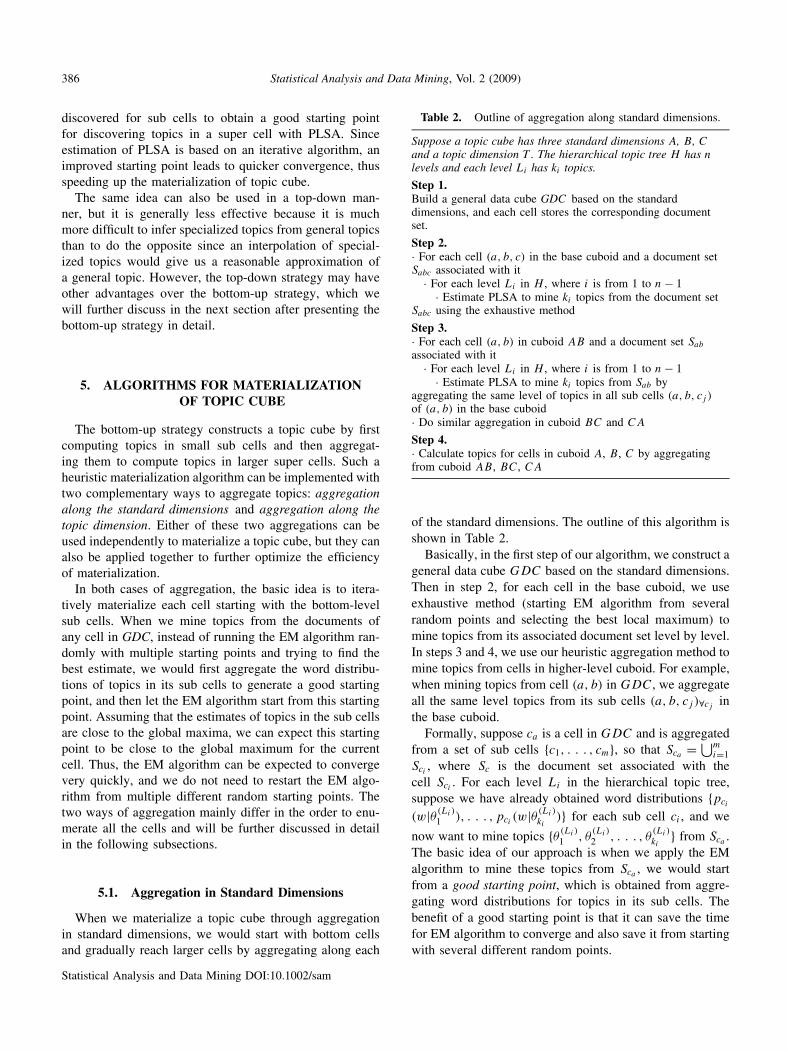
When we materialize a topic cube through aggregationin standard dimensions, we would start with bottom cellsand gradually reach larger cells by aggregating along each

Table 2. Outline of aggregation along standard dimensions.

Suppose a topic cube has three standard dimensions A, B, Cand a topic dimension T . The hierarchical topic tree H has n

levels and each level Li has ki topics.

Step 1.Build a general data cube GDC based on the standarddimensions, and each cell stores the corresponding documentset.

Step 2.· For each cell (a, b, c) in the base cuboid and a document setSabc associated with it

· For each level Li in H , where i is from 1 to n − 1· Estimate PLSA to mine ki topics from the document set

Sabc using the exhaustive method

Step 3.· For each cell (a, b) in cuboid AB and a document set Sab

associated with it· For each level Li in H , where i is from 1 to n − 1

· Estimate PLSA to mine ki topics from Sab byaggregating the same level of topics in all sub cells (a, b, cj )of (a, b) in the base cuboid· Do similar aggregation in cuboid BC and CA

Step 4.· Calculate topics for cells in cuboid A, B, C by aggregatingfrom cuboid AB, BC, CA

of the standard dimensions. The outline of this algorithm isshown in Table 2.

Basically, in the first step of our algorithm, we construct ageneral data cube GDC based on the standard dimensions.Then in step 2, for each cell in the base cuboid, we useexhaustive method (starting EM algorithm from severalrandom points and selecting the best local maximum) tomine topics from its associated document set level by level.In steps 3 and 4, we use our heuristic aggregation method tomine topics from cells in higher-level cuboid. For example,when mining topics from cell (a, b) in GDC, we aggregateall the same level topics from its sub cells (a, b, cj )∀cj

inthe base cuboid.

Formally, suppose ca is a cell in GDC and is aggregatedfrom a set of sub cells {c1, . . . , cm}, so that Sca = ⋃m

i=1Sci

, where Sc is the document set associated with thecell Sci

. For each level Li in the hierarchical topic tree,suppose we have already obtained word distributions {pci

(w|θ(Li)

1 ), . . . , pci(w|θ(Li)

ki)} for each sub cell ci , and we

now want to mine topics {θ(Li)

1 , θ(Li)

2 , . . . , θ(Li )

ki} from Sca .

The basic idea of our approach is when we apply the EMalgorithm to mine these topics from Sca , we would startfrom a good starting point, which is obtained from aggre-gating word distributions for topics in its sub cells. Thebenefit of a good starting point is that it can save the timefor EM algorithm to converge and also save it from startingwith several different random points.



The aggregation formulas are as follows:

p(0)ca

(w|θ(Li)

j ) =∑

ci

∑d∈Sci

c(w, d)p(zd,w = j)∑

w′∑

ci

∑d∈Sci

c(w′, d)p(zd,w′ = j)

p(0)ca

(θ(Li )

j |d) = pci(θ

(Li)

j |d), if d ∈ Sci(5)

Intuitively, we simply pool together the expected countsof a word from each sub cell to get an overall count of theword for a topic distribution. An initial distribution esti-mated in this way can be expected to be closer to the opti-mal distribution than a randomly picked initial distribution.

5.2. Aggregation in Topic Dimension

Similarly, the basic idea of aggregation along the topicdimension is: for each cell in GDC, when we mine topicslevel by level in the hierarchical topic tree in a bottom-upmanner, we would compute the topics in the higher levelof the hierarchical topic tree by first aggregating the worddistributions of the topics in the lower level. The purpose isagain to find a good starting point to run the EM algorithmso that it can converge more quickly to an optimal estimate.The outline of this algorithm is shown in Table 3.

Basically, after constructing a general data cube GDCbased on the standard dimensions, we can use the heuristicaggregation along the topic dimension to mine a hierarchyof topics for each cell. For the topics in the lowest level,we just use PLSA to mine them from scratch. Then, we canmine topics in a higher level in the hierarchical topic treeby aggregating from the lower-level topics.

Formally, suppose cell c has a set of documents S

associated with it, and we have obtained word distributionsfor topics {θ(L+1)

1 , θ(L+1)2 , . . . , θ

(L+1)kL+1

} in level L + 1. Nowwe want to calculate the word distributions for topics

Table 3. Outline of aggregation along the topic dimension.

Suppose a topic cube has several standard dimensions and atopic dimension T . The hierarchical topic tree H has n levelsand each level Li has ki topics.

Step 1.Build a general data cube GDC based on the standarddimensions, and each cell stores the corresponding documentset.

Step 2.· For each cell in GDC and a document set S associated with it

· Estimate PLSA to mine kn−1 topics in the lowest level Ln−1of H from the document set S using exhaustive method

Step 3.· For each cell in GDC and a document set S associated with it

· For each level Li in H , where i is from n − 2 to 1· Estimate PLSA to mine ki topics from the document set

S by heuristically aggregating the topics mined in level Li+1

{θ(L)1 , θ

(L)2 , . . . , θ

(L)kL

} in level L. Here, each topic in levelL has some sub-topics (children nodes) in level L + 1,given by:

Children(θ(L)i ) ={θ(L+1)

si, θ

(L+1)si+1 , . . . , θ (L+1)

ei}, ∀1 ≤ i ≤ kL,

where⋃kL

i=1{θ(L+1)si , . . . , θ

(L+1)ei

} = {θ(L+1)1 , . . . , θ

(L+1)kL+1

}We can use the following formulas to compute a good

starting point to run the EM algorithm for estimating param-eters:

p(0)c (w|θ(L)

i )

=∑

j ′∈{θ(L+1)si

,. . .,θ(L+1)ei

}∑

d∈S c(w, d)p(zd,w = j ′)∑

w′∑

j ′∈{θ(L+1)si

,. . .,θ(L+1)ei

}∑

d∈S c(w′, d)p(zd,w′ = j ′)

p(0)c (θ

(L)i |d) =

∑

θj ′ ∈{θ(L+1)si

,. . .,θ(L+1)ei

}p(θj ′ |d), ∀d ∈ S

(6)

The intuition is similar: we pool together the expectedcounts of a word from all the sub-topics of a super topicto get an overall count of the word for estimating the worddistribution of the super topic. After the initial distributionis calculated, we can run the EM algorithm, which wouldconverge much more quickly than starting from a randominitialization since the initialization point obtained throughaggregation is presumably already very close to the optimalestimate.

5.3. Combination of Two Aggregation Strategies

The two aggregation strategies described above can beused independently to speed up the materialization ofa topic cube. Interestingly, they can also be combinedtogether to further improve the efficiency of materializing atopic cube. Depending on the order of the two aggregationsin their combination, the combination strategy can have twoforms:

(1) First aggregating along the topic dimension and thenaggregating along the standard dimensions: For each cellin the base cuboid of a general data cube GDC, we wouldfirst exhaustively mine the topics in the lowest level ofthe hierarchical topic tree using PLSA. Then, we aggregatealong the topic dimension and get all the topics for cellsin the base cuboid. After that, we can materialize all theother cells through aggregation along the standard dimen-sions to construct a topic cube. This combination strategywould lead to an algorithm very similar to the one shownin Table 2 except that we would change Step 2 to ‘usingthe aggregation along the topic dimension to mine topicsfor each cell in the base cuboid’.



(2) First aggregating along the standard dimensions andthen aggregating along the topic dimension: For each cellin the base cuboid of a general data cube GDC, we wouldfirst exhaustively mine the topics in the lowest level ofthe hierarchical topic tree using PLSA. Then, we aggregatealong the standard dimensions and get the lowest leveltopics for all the cells. After that, for each cell we canuse the aggregation along the topic dimension to mineall the topics of other levels in the hierarchial topic tree.The algorithm for this combination can be illustrated bymodifying Table 3 in which we would change Step 2 to‘using the aggregation along the standard dimensions tomine the lowest level topics for each cell in GDC ’.

The common part of these two different combinations isthat they both need to use PLSA to exhaustively mine thetopics in the lowest level of the hierarchical topic tree for allthe cells in the base cuboid of GDC. After that, they will goalong different directions. One interesting advantage of thesecond combination is that it can be used for materializinga topic cube in a parallel way. Specifically, after we get thelowest level topics for each cell in GDC, we can carry outthe aggregation along the topic dimension for each cell inGDC independently. Therefore, Step 3 in Table 3 can bedone in parallel.

5.4. Saving Storage Cost

One critical issue about topic cube is its storage. As dis-cussed in Section 4.2, for a topic cube with d standarddimensions, we have totally (

∑L1l=1 n

(l)1 ) × · · · × (

∑Ld

l=1 n(l)d )

cells in GDC. If there are N topic nodes in the hierarchi-cal topic tree and the vocabulary size is V , then we need atleast store (

∑L1l=1 n

(l)1 ) × · · · × (

∑Ld

l=1 n(l)d ) × N × V values

for the word distribution measure. This is a huge storagecost because both the number of cells and the size of thevocabulary are large in most cases.

There are three possible strategies to solve the storageproblem. One is to reduce the storage by only storing the topk words for each topic. This method is reasonable, becausein a word distribution of one topic, the top words alwayshave the most information of a topic and can be used torepresent the meaning of the topic. Although the cost of thismethod is the loss of information for topics, this strategyreally saves the disk space a lot. For example, generallywe always have 10000 words in our vocabulary. If we onlystore the top 10 words of each topic in the topic cube insteadof storing all the words, then it will save thousands of timesin disk space. The computational efficiency of this methodis studied in our experiment part.

Another possible strategy is to use a general term toreplace a set of words or phrases so that the size of thevocabulary will be compressed. For example, when we talk

about an engine problem, words or phrases like ‘high tem-perature, noise, left engine, right engine’ always appear.So it motivates us to use a general term ‘engine problem’to replace all those correlated words or phrases. Such areplacement is meaningful especially when an expert onlycares about general causes of an aviation anomaly insteadof the details. But the disadvantage of this method is thatit loses much detailed information, so there is a trade offbetween the storage and the precision of the informationwe need.

The third possible strategy is that instead of storing topicsin all the levels in the hierarchical topic tree, we can selectsome levels of topics to store. For example, we can storeonly the topics in the odd levels or the topics in the evenlevels. The intuition is: suppose one topic’s parent topicnode has a word w at the top of its word distribution and atthe same time its child topic node also has the same word w

at the top of its word distribution, then it is highly probablythat this topic also has word w at the top of its worddistribution. In other words, for a specific topic, we can usethe word distribution in both its parent topic and child topicto quickly induce its own word distribution. For anotherexample, based on users’ query history, we can also selectthose top popular topics to store, which means we only storethe word distribution of mostly queried topics for each cell.For those non-frequently queried topics, they may be justasked for a few times and within some specified cells, e.g.,cells with a specified time period or a specified location.For these cases, we can just calculate the topics online andstore the word distribution for these specified cells. By thisstrategy, it can help us to save a lot of disk spaces.

5.5. Partial Materialization in Top-Down Strategy

Another possible strategy to materialize a topic cube isto compute it in a top-down manner. Specifically, with thisstrategy we would first mine all the topics in the hierarchi-cal tree from the largest cell (also called apex cell) in GDC.Then, in order to compute the topics in the sub cells of anapex cell, we would use the computed word distributionsof topics in the apex cell as starting points and mine topicsin the sub cells individually. After the sub cells of the apexcell are materialized, we can further compute the sub subcells of the apex cell, and the word distributions of topics intheir respective super cells will be used as starting points.This process will be continued iteratively until the wholetopic cube is materialized.

For example, if we want to materialize a topic cube asshown in Fig. 3 in a top-down strategy, we would first mineall the topics in the apex cell of GDC, which is (Location =‘*’, Time = ‘*’). Then, we use the word distribution of themined topics as starting points to mine topics in its sub cells,like (Location = ‘CA’, Time = ‘*’) and (Location = ‘*’,



Time = ‘1999’). After that, we can use the word distribu-tion of topics in a new computed cell, like (Location =‘CA’, Time = ‘*’), as the starting points to mine topics inits sub cells, like (Location = ‘CA’, Time = ‘1999’) and(Location = ‘CA’, Time = ‘1998’). Note that if we do notuse the word distribution of topics in a super cell as start-ing points when mining topics in sub cells, this strategybecomes an exhaustive top-down materialization method.

Since the materialization of a topic cube starts from thelargest cell rather than the smallest cells in GDC, oneadvantage of the top-down strategy over the bottom-upstrategy is that we can stop materializing a topic cube at acertain level of cuboid in GDC if we believe that the cur-rent cuboid is too specific to be mined. This is reasonablebecause of two facts. First, when a cell is very specific, thenumber of documents contained in this cell will be small,which means this cell does not need to be mined or can bemined online, thus no need to materialize. Second, in mostcases, users are interested in analyzing large and generalcells in a cube rather than very specific cells. For example,suppose we have more than 20 standard dimensions in aGDC. When a user inputs a query (a1, a2, . . . , a20, t), shemay only specify the value for a small number of ai’s andset all the other dimensions as ‘*’. Indeed, it is generallydifficult for users to specify the values of all the dimensionsin a data cube. Therefore, in a top-down strategy, not allthe cells in GDC need to be materialized. This can alsosave a lot of disk cost of a topic cube.

However, the idea of leveraging the word distributionsobtained for existing cells to obtain a good starting point forthe EM algorithm would not work as well as in the case ofbottom-up materialization, which is a main disadvantage ofthe top-down strategy. Indeed, using the word distributionsof topics in a super cell as the starting points for miningtopics in its sub cells is generally not very effective becausea super cell is generally made of a number of sub cells, andthe topics embedded in the documents of a single sub cellcan be very different from the super cell. For example, ifone sub cell A contains much smaller number of documentsthan its super cell, the topics mined in this super cell wouldlikely be dominated by the other sub cells of the super cell.As a result, the word distributions of these topics wouldnot be much different from random starting points for sub

cell A. In contrast, in the bottom-up strategy, the startingpoint (e.g., calculated by Eq. 5) during estimating the top-ics in a super cell is a weighted combination of topics inall the sub cells, which can be expected to approximate anoptimal estimate well.

6. EXPERIMENTS

In this section, we present our evaluation of the topiccube model. First, we compare the computation efficiencyof the proposed heuristic materialization methods with abaseline method which materializes a topic cube exhaus-tively cell by cell. Next, we will show several applicationsof topic cube to demonstrate its great potential of usages.

6.1. Data Set

The data set we used in our experiment is downloadedfrom the ASRS database [10]. Three fields of the databaseare used as our standard dimensions, namely, Time {1998,1999}, Location {CA, TX, FL}, and Environment {Night,Daylight}. We use A, B, C to represent them, respectively.Therefore, in the first step, the constructed general datacube GDC has 12 cells in the base cuboid ABC, 16 cellsin cuboids {AB, BC, CA}, and 7 cells in cuboids {A, B,C}. A summary of the number of documents in each basecell is shown in Table 4.

Three levels of hierarchical topic tree are used in ourexperiment: 6 topics in the first level and 16 topics inthe second level as shown in Fig. 5. In real applica-tions, the prior knowledge of each topic can be given bydomain experts. For our experiments, we first collect a largenumber of aviation safety report data (also from ASRS

Table 4. The number of documents in each base cell.

CA TX FL

1998 Daylight 456 306 2661998 Night 107 64 621999 Daylight 493 367 3211999 Night 136 87 68

Level 0 ALL

Level 1EquipmentProblem Altitude Deviation Conflict

GroundIncursion

In-FlightEncounter

MaintainProblem

Level 2Critical,Less Severe

Crossing RestrictionNot Meet,Excursion FromAssigned Altitude,Overshoot, Undershoot

Airborne,Ground,NMAC*

Landing WithoutClearance,Runway

Turbulence,VFR* in IMC*,Weather

ImproperDocumentation,ImproperMaintenance

∗: NMAC-Near Midair Collision, VFR-Visual Flight Rules, IMC-Instrument Meteorological Conditions

Fig. 5 Hierarchical topic tree used in the experiments.



0.24 0.23 0.22 0.21 0.2 0.19 0.18 0.17 0.16 0.15 0.14

10

20

30

40

50

60

70

80

90

Closeness to Global Optimum Point (%)

Sec

onds

AggAppBest RdmAvg Rdm

0.5 0.46 0.42 0.38 0.35 0.31 0.27 0.23 0.2 0.160

20

40

60

80

100

120

140

160

180

Closeness to Global Optimum Point (%)S

econ

ds


0.3 0.28 0.26 0.24 0.22 0.2 0.18 0.16 0.14 0.12

50

100

150

200

250

300

350

400

450


Sec

onds


(a) Cell = (1999, CA, *)with 629 documents

(b) Cell = (1999, *, *)with 1472 documents

(c) Cell = (*, *, *)with 2733 documents

Using aggregation along the standard dimensions

0.25 0.24 0.23 0.22 0.21 0.2 0.19 0.18 0.18 0.17

10

20

30

40

50

60

70

80


Sec

onds


0.95 0.91 0.86 0.82 0.77 0.73 0.68 0.63 0.59 0.54 0.5 0.4510

15

20

25

30

35

40

45

50


Sec

onds


0.93 0.88 0.83 0.79 0.74 0.69 0.64 0.6 0.55 0.5 0.450

10

20

30

40

50

60

70

Closeness to Global Optimum Point (%)S

econ

ds


(d) Cell = (1999, CA, *)with 629 documents

(e) Cell = (1999, *, *)with 1472 documents

(f) Cell = (*, *, *)with 2733 documents

Using aggregation along the topic dimension

Fig. 6 Efficiency comparison of different strategies for aggregation in standard dimensions (top) and topic dimension (bottom).

database), and then manually check documents related toeach anomalous event, and select top k (k < 10) most rep-resentative words of each topic as its prior.

6.2. Efficiency Comparison

In this section, we evaluate the efficiency of the twoheuristic aggregation strategies proposed in Section 5 andcompare each with the corresponding baseline method. Foreach aggregation method, we compare three strategies ofconstructing a topic cube.(1) The heuristic aggregation method we proposed (eitheraggregation along the topic dimension or aggregation alongthe standard dimensions), which will be represented as Agg.(2) An approximation method which only stores top k

words in the word distribution of each topic and will berepresented as App. The purpose of this method is to testthe storage-saving strategy proposed in Section 5.4. Forexample, in aggregation along standard dimensions, whencalculating topics from a document set in one cell, we usethe same formula as in Agg to combine the word distribu-tions of topics in its sub cells, but with only top k words,to get a good starting point. Then, we initialize the EM

algorithm with this starting point and run it until conver-gence. Similarly, in aggregation along the topic dimension,we also use only the top k words in the lower-level topics toaggregate a starting point when we estimate the topics in thehigher level. In our experiments, we set the constant k to 10.(3) The baseline method, which initializes the EM algorithmwith random points and will be represented as Rdm. Asstated before, the exhaustive method to materialize a topiccube runs EM algorithm by starting from several differentrandom points and then selecting the best local maximumpoint. Obviously, if the exhaustive method runs EM algo-rithm M times, its time cost will be M times of the Aggmethod. The reason is every run of EM algorithm in Rdmhas the same computation complexity as the Agg method.Therefore, it is not surprising that the heuristic aggrega-tion method is faster than the exhaustive method. Thus, inour experiment, we use both the average performance andbest performance from a single run of the random methodto compare the efficiency with the Agg method. The aver-age performance is calculated by running the EM algorithmfrom M random points and then averaging the performanceof these runs. The best performance is computed using the



single best run that converges to the best local optimumpoint (highest log likelihood) among these M runs.

To measure the efficiency of these strategies, we look athow long it takes for these strategies to get to the samecloseness to the global optimum point. Here, we assumethat the convergence point of the best run of the M randomruns is the global optimum point. The experimental resultsare shown in Fig. 6. The upper three graphs show theefficiency comparison among the different strategies usingaggregation along the standard dimensions, and the topicswe computed in these three graphs are the 16 topics in thelowest level of the hierarchical topic tree in Fig. 5. Eachgraph represents the result in one level of cuboid in theGDC cube, and we use one representative cell to show thecomparison. The experiments on other cells have similarperformance and can lead to the same conclusion. Similarly,the lower three graphs show the efficiency comparisonusing aggregation along the topic dimension, and the topicswe computed are the six topics in the second level of thehierarchical topic tree.

In the graph, Best Rdm represents the best run amongthose M random runs in the third strategy, and Avg Rdmrepresents the average performance of the M runs. The hor-izontal axis represents how close one point is to the globaloptimum point. For example, the value ‘0.24’ on the axismeans one point’s log likelihood is 0.24% smaller than thelog likelihood of the global optimum point. The verticalaxis is the time measured in seconds. So a point in theplane means how much time a method needs to get to acertain closeness to the global optimum point. We can con-clude that in all three cells, the proposed heuristic methodsperform more efficiently than the baseline method, and thisadvantage of the heuristic aggregation is not affected bythe scale of the document set. An interesting discovery isthat the App method performs comparably with the Aggmethod, and in some cases it is even more stable than Agg.For example, in Fig. 6(b) and (c), although the Agg methodstarts from a better point than App, after reaching a certainpoint, the Agg method seems to be ‘trapped’ and needslonger time than App to get further close to the optimumpoint.

Table 5 shows the log likelihood of the starting points ofthe three strategies. Here, the log likelihood of the objectivefunction is calculated by Eq. 1. This value indicates howlikely the documents are generated by topic models, sothe larger, the better. In all the cells, both Agg and Appstrategies (in both two kinds of aggregations) have highervalue than the average value of the Rdm strategy, whichfurther supports our hypothesis that the starting points usedin the proposed heuristic methods are closer to the optimumpoint than a random starting point, and thus our methodsneed less time to converge.

Table 5. Comparison of starting points in different strategies.

Aggregation along the standard dimensions

Strategy (1999, CA, *) (1999, *, *) (*, *, *)Agg −501 098 −1 079 750 −2 081 270App −517 922 −1 102 810 −2 117 920Avg Rdm −528 778 −1 125 987 −2 165 459Best Rdm −528 765 −1 125 970 −2 165 440

Aggregation along the topic dimension

Strategy (1999, CA, *) (1999, *, *) (*, *, *)Agg −521 376 −1 111 400 −2 135 910App −524 781 −1 116 220 −2 144 730Avg Rdm −528 796 −1 126 046 −2 165 551Best Rdm −528 785 −1 126 040 −2 165 510

Environment Anomaly Event Word Distribution

daylightlanding without

clearancetower 0.075, pattern 0.061, final 0.060,

runway 0.052, land 0.051, downwind 0.039

nightlanding without

clearancetower 0.035, runway 0.027, light 0.026, lit

0.014, ils 0.014, beacon 0.013

daylightaltitude deviation:

overshootaltitude 0.116, level 0.029, 10000 0.028, f

0.028,o 0.024, altimeter 0.023

nightaltitude deviation:

overshootaltitude 0.073, set 0.029, altimeter 0.022,

level 0.022, 11000 0.018, climb 0.015

Fig. 7 Application of topic cube in ASRS.

6.3. Topic Comparison in Different Context

One major application of a topic cube is to allow users toexplore and analyze topics in different contexts. Here, weregard all the standard dimensions as contexts for topics.Figure 7 shows four cells in the topic cube constructed onour experiment data. The column of ‘Environment’ can beviewed as the context of the topic dimension ‘AnomalyEvent’. Comparing the same topic in different contextswill discover some interesting knowledge. For example,from the figure we can see that the ‘landing without clear-ance’ anomaly has more emphasis on the words ‘light’,‘ils’(instrument landing system), and ‘beacon’ in the con-text of ‘night’ than in the context of ‘daylight’. This tellsexperts of safety issues that these factors are most impor-tant for landing and are mentioned a lot by pilots. On theother hand, the anomaly ‘altitude deviation: overshoot’ isnot affected too much by the environment light, becausethe word distribution in these two contexts is quite similar.

6.4. Topic Coverage in Different Context

Topic coverage analysis is another application of a topiccube. As described above, one family of parameters inPLSA, {p(θ |d)}, is stored as an auxiliary measure in a topiccube. These parameters indicate the topic coverage in eachdocument. With this family of parameters, we can analyzethe topic coverage in different context. For example, givena context (Location=‘LA’, Time=‘1999’), we can calculate



(a) Place Comparison (b) Environment Comparison

Improper MaintenanceImproper Documentation

WeatherVFR in IMCTurbulence

RunwayLanding without clearance

NMACGround

AirborneUndershoot

OvershootExcursion From Assigned Altitude

Crossing Restriction Not MeetLess Severe

Critical

Improper MaintenanceImproper Documentation

WeatherVFR in IMCTurbulence

RunwayLanding without clearance

NMACGround

AirborneUndershoot

OvershootExcursion From Assigned Altitude

Crossing Restriction Not MeetLess Severe

Critical

0.00% 2.00% 4.00% 6.00% 8.00% 10.00% 12.00% 0.00% 2.00% 4.00% 6.00% 8.00% 10.00% 12.00%14.00%

FL

TX

CA

Daylight

Night

Fig. 8 Topic coverage comparison among different contexts.

Table 6. Examples and keyword lists of shaping factors.

Shaping factors Example Keyword list

Preoccupation My attention was divided inappropriately distraction, attention, busy, emergency, realize,focus, declare

Communication environment We were unable to hear because traffic alert andcollision avoidance system was very loud

communication, clearance, radio, frequency,hear, unreadable, wait

Familiarity Both pilots were unfamiliar with the airport unfamiliar, new, before, line, familiar,inexperienced, time

Physical environment This occurred because of the intense glare of the sun weather, snow, cloud, wind, condition, ice,visibility

Physical factors I allowed fatigue and stress to cloud my judgment fatigue, leg, hours, night, day, tire, rest

the coverage or proportion of one topic t by the average ofp(t |di) over all the document di in the corresponding cellin GDC. From another point of view, the coverage of onetopic also reflects the severity of this anomaly.

Figure 8 shows the topic coverage analysis on our exper-iment data set. Figure 8(a) is the topic coverage over differ-ent places and Fig. 8(b) is the topic coverage over differentenvironment. With this kind of analysis, we can easily findout answers to questions such as ‘What is the most severeanomaly among all the flights in California state?’, ‘Whatkind of anomaly is more likely to happen during night ratherthan daylight?’. For example, Fig. 8 reveals some veryinteresting facts. Flights in Texas have more ‘turbulence’problems than in California and Florida, whereas Floridahas the most severe ‘Encounter: Airborne’ problem amongthese three places, and there is no evident difference of thecoverage of anomalies such as ‘Improper documentation’between night and daylight. This indicates that these kindsof anomalies are not correlated with environment factorsvery much. On the other hand, anomaly ‘Landing with-out clearance’ obviously has a strong correlation with theenvironment.

6.5. Shaping Factor Analysis

Analyzing the shaping factors of human performanceduring flights plays an important role in aviation safety

research. The reporters of anomalous events tend to describetheir physical factors, attitude, pressure, proficiency, preoc-cupation, etc., in the text reports, which can be potentialcauses of an anomalous event. Thus, it is necessary to ana-lyze all these factors in text and their correlations withanomalies. With a topic cube, we can quantitatively evalu-ate the correlations between the anomalous events and theshaping factors of human performance in different context.Table 6 shows five different shaping factors as well as someexamples and keywords describing them.

To support shaping factor analysis, we first extract key-word lists for describing shaping factors as follows. First, ahuman annotator is hired to annotate 1333 incident reportswith 14 different shapers, where each report can be labeledwith one or more shapers. Given the labeled reports, infor-mation gain [37] is used to compute a score for eachunigram and each shaper. The top-k highest scored uni-grams are selected as the keyword list for each shaper1. Toquantitatively evaluate the correlation between a shaper S

and an anomaly A in a specific context C, we first find theword distribution in the cell specified by A and C in a topiccube. Then, the correlation value is calculated as the sumover all the keywords in S based on their probabilities inthe word distribution.

1 We would like to thank Professor Vincent Ng from UT Dallasfor providing us the keyword lists of shapers.



(a) Texas (b) FloridaShaper analysis in different places

(c) Night (d) Daylight

Shaper analysis in different environment

2.50E-02

2.00E-02

1.50E-02

1.00E-02

5.00E-03

0.00E+00

2.50E-02

3.00E-02

2.00E-02

1.50E-02

1.00E-02

5.00E-03

0.00E+00

5.00E-02

6.00E-02

4.00E-02

3.00E-02

2.00E-02

1.00E-02

0.00E+00

5.00E-02

6.00E-02

7.00E-02

4.00E-02

3.00E-02

2.00E-02

1.00E-02

0.00E+00

Communication Environment

Physical Environment

Familiarity

Physical Factors

Preoccupation



Familiarity

Physical Factors

Preoccupation



Familiarity

Physical Factors

Preoccupation



Familiarity

Physical Factors

Preoccupation

Fig. 9 Shaper analysis in different context.

Figure 9 shows some examples of shaping factor analy-sis in different context based on a topic cube. The x-axis ineach graph represents different anomalous events, and they-axis represents the correlation between shaping factorsand anomalous events (since the correlation is calculatedas the sum over the probabilities of keywords of a shapergiven the anomalous events, the value is relatively smallas shown in the figure). From these graphs, we can findthat ‘physical environment’ is the main cause for anoma-lous events ‘Weather’ and ‘VFR in IMC’, no matter whatthe context is. This is consistent with our common sense.On the other hand, if we look into the difference of the cor-relations among different contexts, we can also make someinteresting observations. For example, the shaping factor‘Physical factors’ causes more anomaly during night ratherthan daylight. The shaping factor ‘communication envi-ronment’ causes the ‘Landing without clearance’ anomalymuch more in Texas than in Florida, which suggests thatairports or aircrafts in Texas may need to improve theircommunication environment.

6.6. Accuracy of Categorization

In this experiment, we test how accurate the topicmodeling method is for document categorization. Sincewe only have our prior for each topic without train-ing examples in our data set, we do not compare ourmethod with supervised classification methods. Instead, weuse the following method as our baseline. First, we usethe prior of each topic to estimate a language model φj

for each topic j . Then, we create a document languagemodel ζd for each document with Dirichlet smoothing:p(w|ζd) = (c(w, d) + µp(w|C))/(|d| + µ), where c(w, d)

is the count of word w in document d and p(w|C) =(c(w, C))/(

∑w′ c(w′, C)) is the collection background

model. Finally, we can use the negative KL-divergence[38] function to measure the similarity between a doc-ument d and a topic j : S = −D(φj‖ζd) = ∑

w p(w|φj )

log(p(w|ζd))/(p(w|φj )). If document d has a similarityscore S higher than a threshold δ with a topic j , it wouldbe classified into topic j . On the other hand, when weuse the word distribution measure in a topic cube for cat-egorization, we use the word distribution θj of topic j



0 0.1 0.2 0.3 0.4 0.5 0.6 0.7 0.8 0.9 10.2

0.3

0.4

0.5

0.6

0.7

0.8

0.9

Recall

Pre

cisi

on

BaselinePLSA

Fig. 10 Comparison of categorization accuracy .

as its language model, and then compute the negativeKL-divergence between θj and ζd to compute the similarityscore of each topic j and document d. The idea is to seewhether the estimated topic model (i.e., θj ) in a topic cubeworks better for categorizing documents than the originaltopic language model φj .

Our experiment is conducted on the whole data set,and we used the first level of topics in Fig. 5 as thetarget categories, i.e., we classify the documents into sixcategories. The gold standard is the ‘Anomaly Event’ labelsprovided in the ASRS data. We plot the recall-precisioncurves by changing the value of the threshold δ in Fig. 10.From this figure, we can see that the curve of PLSA is abovethe baseline method, meaning that the topic representationobtained in the topic cube through PLSA can indeed achievebetter categorization results than if we only use the priorknowledge about topics.

7. CONCLUSIONS

OLAP is a powerful technique for mining structured data,whereas probabilistic topic models are among the mosteffective techniques for mining topics in text and analyzingtheir patterns. In this paper, we proposed a new data model(i.e., topic cube) to combine OLAP and topic models sothat we can extend OLAP to the text dimension whichallows an analyst to flexibly explore the content in textdocuments together with other standard dimensions in aMTD. Technically, we extended the standard data cube intwo ways: (i) adopt a hierarchical topic tree to define atopic dimension for exploring text information, and (ii)store word distributions as the primary content measure(and topic coverage probabilities as auxiliary measure) oftext information. All these probabilities can be computed

simultaneously through estimating a probabilistic latentsemantic analysis model based on the text data in a cell. Toefficiently materialize topic cube, we propose two kinds ofheuristic aggregations which leverage previously estimatedmodels in component cells or lower-level topics to choosea good starting point for estimating the model for a mergedlarge cell or higher-level topics. Experimental results showthat the heuristic aggregations are effective and topic cubecan be used for many different applications.

Our work is only the first step in combining OLAP withtext mining based on topic models, and there are manyinteresting directions for further study. First, it is necessaryto further explore other possible strategies to materializea topic cube efficiently, e.g., the top-down strategy dis-cussed in Section 5. Second, it would be interesting toexplore more application tasks to take advantage of therich intermediate results of text analysis provide by a topiccube, and compare the topic cube with a baseline method,where OLAP on structured data and text mining are doneseparately, to verify its effectiveness in supporting an appli-cation task. Finally, our work only represents one way tocombine OLAP and topic models. It should be very inter-esting to explore other ways to integrate these two kinds ofeffective, yet quite different mining techniques.

Acknowledgment

The work was supported in part by NASA grantNNX08AC35A, the U.S. National Science Foundationgrants IIS-0842769, IIS-0713571, and IIS-0713581, andthe Air Force Office of Scientific Research MURI awardFA9550-08-1-0265.

REFERENCES

[1] S. Agarwal, R. Agrawal, P. Deshpande, A. Gupta,J. F. Naughton, R. Ramakrishnan, and S. Sarawagi, On thecomputation of multidimensional aggregates, in Proceedingsof the VLDB Conference, Mumbai, India, 1996, 506–521.

[2] S. Chaudhuri and U. Dayal, An overview of datawarehousing and OLAP technology, SIGMOD, Tucson,Arizona, USA, 26 (1997), 65–74.

[3] J. Gray, A. Bosworth, A. Layman, and H. Pirahesh, Datacube: A relational aggregation operator generalizing group-by, cross-tab, and sub-totals, Proceedings of the ICDE, NewOrleans, LA, USA, 1996, 152–159.

[4] F. M. fei Jiang, J. Pei, and A. W. chee Fu, Ix-cubes: icebergcubes for data warehousing and OLAP on xml data, inCIKM ‘07: Proceedings of the Sixteenth ACM conferenceon Conference on Information and Knowledge Management,Lisbon, Portugal, 2007, 905–908.

[5] E. Lo, B. Kao, W.-S. Ho, S. D. Lee, C. K. Chui, andD. W. Cheung, OLAP on sequence data, in SIGMOD ’08:Proceedings of the 2008 ACM SIGMOD InternationalConference on Management of Data, Vancouver, Canada,2008, 649–660.



[6] Y. Tian, R. A. Hankins, and J. M. Patel, Efficient aggre-gation for graph summarization, in SIGMOD ’08: Proceed-ings of the 2008 ACM SIGMOD International Conferenceon Management of Data, Vancouver, Canada, 2008,567–580.

[7] B.-C. Chen, L. Chen, Y. Lin, and R. Ramakrishnan,Prediction cubes, in VLDB ’05: Proceedings of the 31stInternational Conference on Very Large Data Bases,Trondheim, Norway, VLDB Endowment, 2005, 982–993.

[8] Y. Chen, G. Dong, J. Han, B. W. Wah, and J. Wang, Multi-dimensional regression analysis of time-series data streams,in Proceedings of the 2002 International Conference onVery Large Data Bases (VLDB’02), Hong Kong, China,August 2002, 323–334.

[9] W. F. Cody, J. T. Kreulen, V. Krishna, and W. S. Spangler,The integration of business intelligence and knowledgemanagement, IBM Syst J, 41 (2002), 697–713.

[10] Aviation safety reporting system. http://asrs.arc.nasa.gov/.[11] Anomaly event schema. http://www.asias.faa.gov/pls/portal/

stage.meta show column?v table id=% 165477.[12] V. T. Chakaravarthy, H. Gupta, P. Roy, and M. Mohania,

Efficiently linking text documents with relevant structuredinformation, in VLDB ’06: Proceedings of the 32ndInternational Conference on Very Large Data Bases, Seoul,Korea, VLDB Endowment, 2006, 667–678.

[13] P. G. Ipeirotis, A. Ntoulas, J. Cho, and L. Gravano,Modeling and managing changes in text databases, ACMTrans Database Syst, 32 (2007), 14.

[14] A. Inokuchi and K. Takeda, A method for online analyticalprocessing of text data, in CIKM ’07: Proceedings of thesixteenth ACM Conference on Information and KnowledgeManagement, Lisbon, Portugal, 2007, 455–464.

[15] J. M. Perez, R. Berlanga, M. J. Aramburu, and T. B.Pedersen, A relevance-extended multi-dimensional modelfor a data warehouse contextualized with documents, inDOLAP ’05: Proceedings of the 8th ACM InternationalWorkshop on Data Warehousing and OLAP, Bremen,Germany, 2005, 19–28.

[16] T. Hofmann, Probabilistic latent semantic indexing, inSIGIR ’99: Proceedings of the 22nd Annual InternationalACM SIGIR Conference on Research and Development inInformation Retrieval, Berkeley, California, USA, ACMPress, 1999, 50–57.

[17] D. M. Blei, A. Y. Ng, and M. I. Jordan, Latent Dirichletallocation, J Mach Learn Res 3 (2003), 993–1022.

[18] T. Hofmann, The cluster-abstraction model: Unsupervisedlearning of topic hierarchies from text data, in Proceedingsof the IJCAI, T. Dean, ed. Stockholm, Sweden, MorganKaufmann, 1999, 682–687.

[19] D. M. Blei, T. L. Griffiths, M. I. Jordan, and J. B.Tenenbaum, Hierarchical topic models and the nestedChinese restaurant process, In Proceedings of the NIPSConference, Vancouver, B.C., Canada, 2003.

[20] M. Steyvers, P. Smyth, M. Rosen-Zvi, and T. Griffiths, Prob-abilistic author-topic models for information discovery, inProceedings of KDD’04, Seattle, WA, USA, 2004, 306–315.

[21] Q. Mei, C. Liu, H. Su, and C. Zhai, A probabilisticapproach to spatiotemporal theme pattern mining onweblogs, in Proceedings of the WWW, L. Carr, D. D.Roure, A. Iyengar, C. A. Goble, and M. Dahlin, eds.Edinburgh, Scotland, ACM, 2006, 533–542.

[22] Q. Mei, X. Ling, M. Wondra, H. Su, and C. Zhai, Topic sen-timent mixture: Modeling facets and opinions in weblogs,

in Proceedings of WWW ’07, Banff, Alberta, Canada,2007.

[23] X. Wang, C. Zhai, X. Hu, and R. Sproat, Mining correlatedbursty topic patterns from coordinated text streams, inProceedings of the KDD, P. Berkhin, R. Caruana, andX. Wu, eds., San Jose, California, USA, ACM, 2007,784–793.

[24] J. Ponte and W. B. Croft, A language modeling approach toinformation retrieval, In Proceedings of the ACM SIGIR’98,Melbourne, Australia, 1998, 275–281.

[25] C. Zhai and J. Lafferty, Model-based feedback in the lan-guage modeling approach to information retrieval, in TenthInternational Conference on Information and KnowledgeManagement (CIKM 2001), Atlanta, Georgia, USA, 2001,403–410.

[26] Q. Mei and C. Zhai, Generating impact-based summariesfor scientific literature, in Proceedings of the 46th AnnualMeeting of the Association for Computational Linguistics,Columbus, Ohio, USA, 2008, 816–824.

[27] Q. Mei, X. Shen, and C. Zhai, Automatic labeling ofmultinomial topic models, in Proceedings of the 14th ACMSIGKDD International Conference on Knowledge Discoveryand Data Mining, San Jose, CA, USA, ACM 2007, 490–499.

[28] N. Bansal and N. Koudas, BlogScope: a system for onlineanalysis of high volume text streams, in VLDB ’07:Proceedings of the 33rd International Conference on VeryLarge Data Bases, Vienna, Austria, VLDB Endowment,2007, 1410–1413.

[29] P. Wu, Y. Sismanis, and B. Reinwald, Towards keyword-driven analytical processing, in SIGMOD ’07: Proceedingsof the 2007 ACM SIGMOD International Conference onManagement of Data, Beijing, China, 2007, 617–628.

[30] Megaputer’s polyanalyst. http://www.megaputer.com/.[31] A. Simitsis, A. Baid, Y. Sismanis, and B. Reinwald,

Multidimensional content exploration, Proc VLDB Endow,1 (2008), 660–671.

[32] C. X. Lin, B. Ding, J. Han, F. Zhu, and B. Zhao, Text cube:Computing IR measures for multidimensional text databaseanalysis, in ICDM ’08: Proceedings of the 2008 EighthIEEE International Conference on Data Mining, Pisa, Italy,2008, 905–910.

[33] D. Zhang, C. Zhai, and J. Han, Topic cube: Topic modelingfor OLAP on multidimensional text databases, in SDM’09:Proceedings of the Ninth SIAM International Conference onData Mining, Sparks, NV, USA, SIAM, 2009, 1124–1135.

[34] D. Blei and J. Lafferty, Correlated topic models, in NIPS ’05:Advances in Neural Information Processing Systems 18,Vancouver, B.C., Canada, 2005.

[35] A. P. Dempster, N. M. Laird, and D. B. Rubin, Maximumlikelihood from incomplete data via the EM algorithm,J Roy Stat Soc B, 39 (1977), 1–38.

[36] T. Tao and C. Zhai, Regularized estimation of mixturemodels for robust pseudo-relevance feedback, in SIGIR ’06:Proceedings of the 29th Annual International ACM SIGIRConference on Research and Development in InformationRetrieval, Seattle, WA, USA, 2006, 162–169.

[37] Y. Yang and J. O. Pedersen, A comparative study onfeature selection in text categorization, in ICML ’97:Proceedings of the Fourteenth International Conference onMachine Learning, Nashville, TN, USA, Morgan KaufmannPublishers Inc., 1997, 412–420.

[38] S. Kullback and R. A. Leibler, On information andsufficiency, Ann Math Stat, 22 (1951), 79–86.


Topic modeling for OLAP on multidimensional text databases: topic cube and its applications

Documents

Transcript of Topic modeling for OLAP on multidimensional text databases: topic cube and its applications