Topic 7 Sampling And Sampling Distributions. The term Population represents everything we want to...
69
Topic 7 Sampling And Sampling Distributions
-
date post
20-Dec-2015 -
Category
Documents
-
view
213 -
download
0
Transcript of Topic 7 Sampling And Sampling Distributions. The term Population represents everything we want to...

Topic 7
Sampling
And
Sampling Distributions

• The term Population represents everything we want to study, bearing in mind that the population is ever changing and hence a dynamic concept.
• A Census is a snapshot of the population at any single point of time.
• For example, the last UK census was taken on the 29th of April 2001.
• The Office of National Statistics (ONS) attempted to get a picture of everything that is relevant on that specific day!
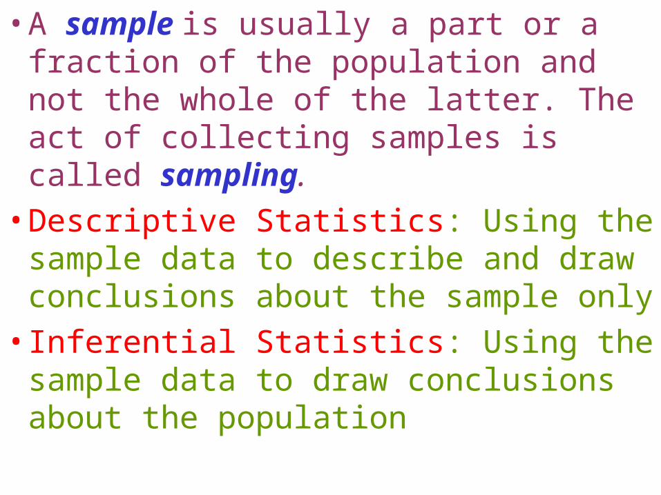
• A sample is usually a part or a fraction of the population and not the whole of the latter. The act of collecting samples is called sampling.
• Descriptive Statistics: Using the sample data to describe and draw conclusions about the sample only
• Inferential Statistics: Using the sample data to draw conclusions about the population

The statistician uses the information out of sample(s) to estimate population characteristics.
Getting access to the entire population may be prohibitively costly and a sample is therefore taken.

• Errors therefore occur naturally.
• A parameter is a defining characteristic of a population that can be quantified.
• The mean and standard deviationof the normal distribution are examples of parameters of the distribution.

•The difference between the actual population characteristic and the corresponding estimate is called a sampling error.
The process can be visualised as below:

Population


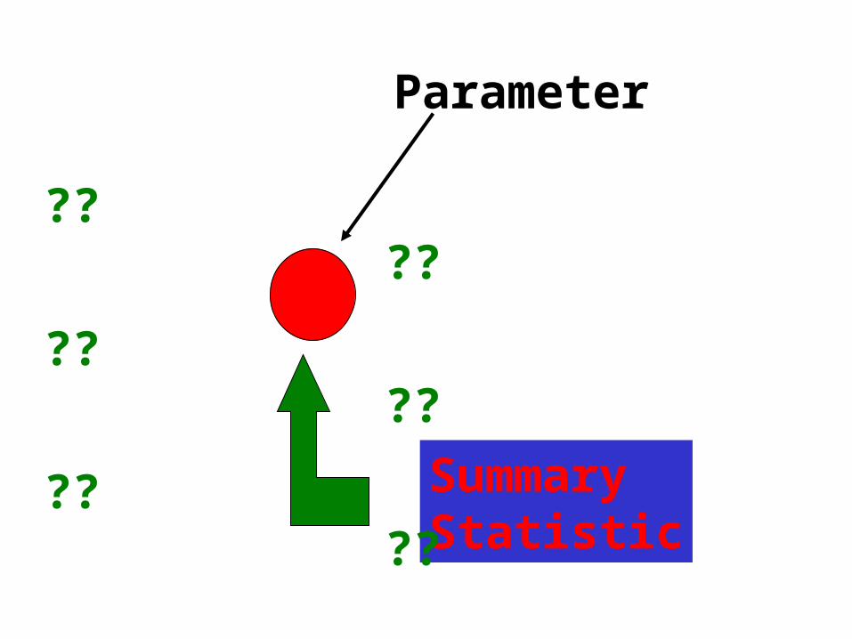
Parameter
SummaryStatistic
?? ??
?? ??
?? ??

Statistic

Learning Objectives
• Determine when to use sampling instead of a census.
• Distinguish between random and nonrandom sampling.
• Be aware of the different types of error that can occur in a study.
• Understand the impact of the Central Limit Theorem on statistical analysis.
• Use the sampling distributions of xMEAN the sample mean and p (the sample proportion).
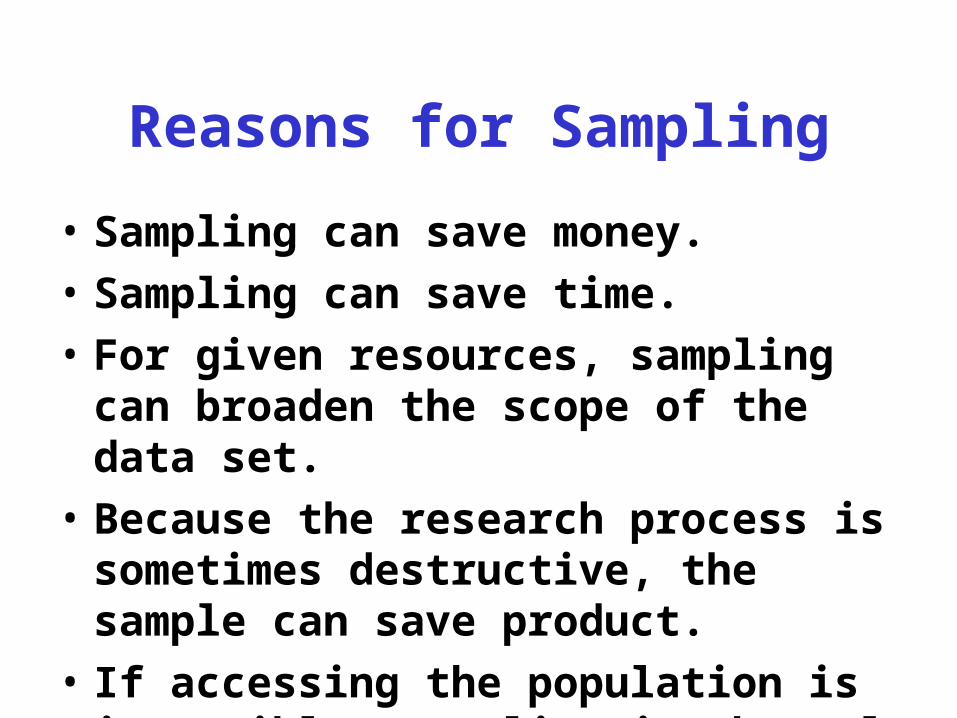
Reasons for Sampling
• Sampling can save money.
• Sampling can save time.
• For given resources, sampling can broaden the scope of the data set.
• Because the research process is sometimes destructive, the sample can save product.
• If accessing the population is impossible; sampling is the only option.

Reasons for Taking a Census
• Eliminate the possibility that a random sample is not representative of the population.
• The person authorizing the study is uncomfortable with sample information.

Random vs Nonrandom SamplingRandom vs Nonrandom Sampling
• Random sampling
• Every unit of the population has the same probability of being included in the sample.
• A chance mechanism is used in the selection process.
• Eliminates bias in the selection process
• Also known as probability sampling

Random vs Nonrandom SamplingRandom vs Nonrandom Sampling
• Nonrandom Sampling
• Every unit of the population does not have the same probability of being included in the sample.
• Open the selection bias
• Not appropriate data collection methods for most statistical methods
• Also known as nonprobability sampling

Data from nonrandom samples are not appropriate for analysis by inferential statistical methods.
Sampling Error occurs when the sample is not representative of the population
Errors

Nonsampling Errors
•Missing Data, Recording, Data Entry, and Analysis Errors
•Poorly conceived concepts , unclear definitions, and defective questionnaires
•Response errors occur when people do not know, will not say, or overstate in their answers

The Central Limit Theorem (CLT)
Whatever the population distribution, the distribution of the sample mean is normal( 2/n )as long as n is ‘large’

Proper analysis and interpretation of a sample statistic requires knowledge of its distribution.
Sampling Distribution of the Sample MeanSampling Distribution of the Sample Mean
Population
(parameter)
Sample
x
(statistic)
Calculate x
to estimate
Select a
random sample
Process ofInferential Statistics
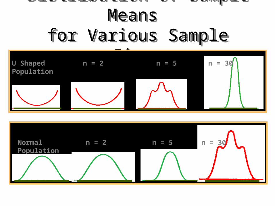
Distribution of Sample Means for Various Sample Sizes
Distribution of Sample Means for Various Sample Sizes
U ShapedPopulation
n = 2 n = 5 n = 30
NormalPopulation
n = 2 n = 5 n = 30

Topic 8
Pointand
Confidence Interval Estimation
The methodology we follow is known as Parametric Analysis
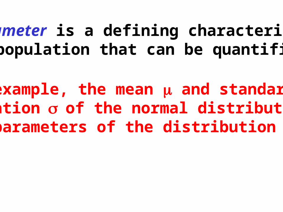
A parameter is a defining characteristicof a population that can be quantified.
For example, the mean and standarddeviationof the normal distributionare parameters of the distribution

Parameter
SummaryStatistic
?? ??
?? ??
?? ??
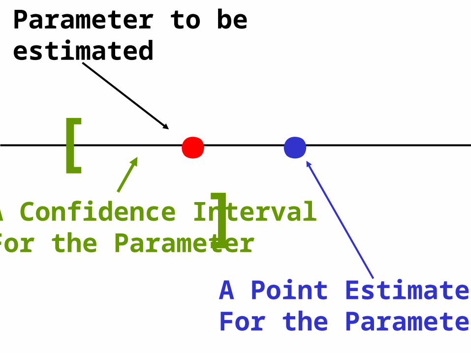
.Parameter to beestimated
.A Point EstimateFor the Parameter
[ ]A Confidence IntervalFor the Parameter
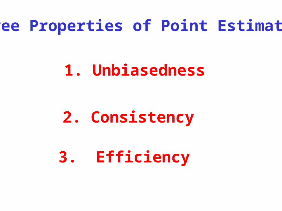
Three Properties of Point Estimators
1. Unbiasedness
2. Consistency
3. Efficiency

Parameter
.. .
...
. .
Estimator
Although each estimator is way off target, together they may well give a good estimation

. .. ... . .. .ParameterReal Line
++ + +
+- - --
(Unknown)
This method of estimation isUnbiased if and onlyif the algebraic sum of all‘errors’ is zero.
Each deviation from the parameter is called an error
And the ‘average’ of these errors isCalled standard error of estimation

.... ..Question: Given the five piece dataset,which point represents thesummary statistic ?
Answer: The sample mean is the bestof all available options

The Sampling Distribution of theSample Mean (xMEAN)
Suppose that the population mean = 20 and consider the following statistical process
Sample Number Value of xMEAN
1 18 2 24 3 21 - -
100 22
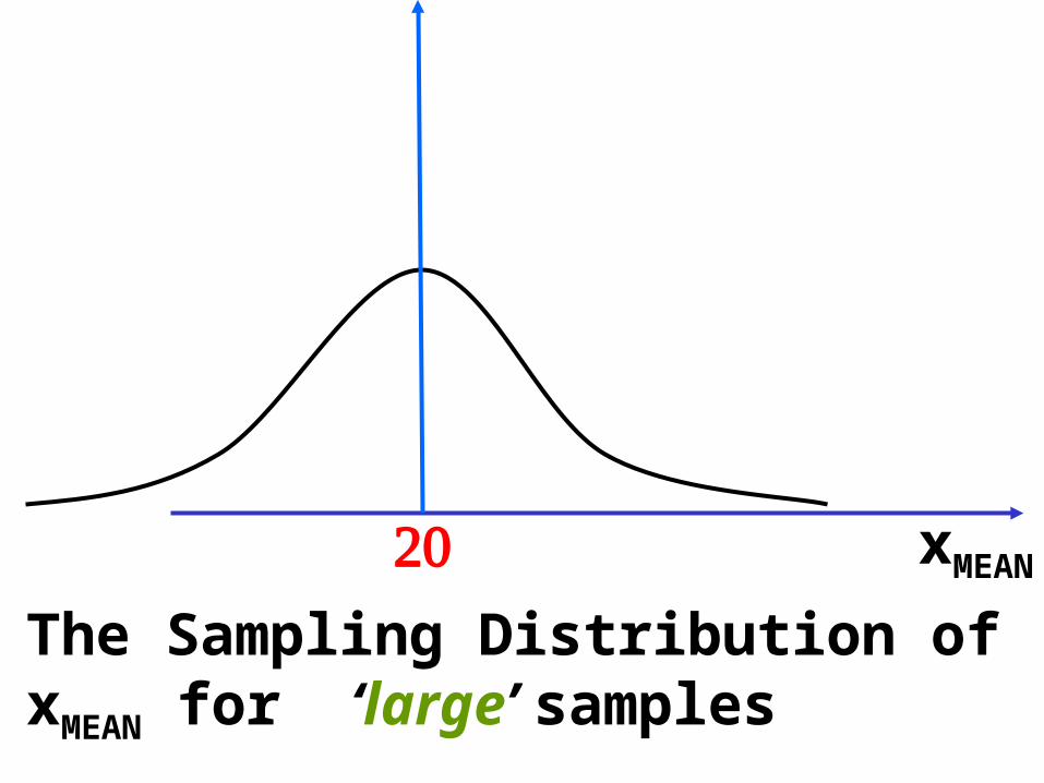
xMEANThe Sampling Distribution ofxMEAN for ‘large’ samples

.. ... ... .. .... ...
. .. .. ..
. Location of Parameter
.Negatively biased estimator
..
...
Positively biased estimatorUnbiased estimator

Estimate Number Error 1 +6 2 +8 3 -10 4 +2 5 -6
Error 0 0 0 -1 0
Although the first set of estimates (in red)have an average of zero, it is probably notas good as the second one (in green)

.. ... . .. .. . ... ...
. ... .. ..
An example of an unbiased yet inefficient estimator
.

. .. ... . .. .
..
.... ... ..
..
... ... ..
Available Resources: R1
Available Resources: R2
Available Resources: R3
This estimator is consistent if R1< R2< R3.

Formally, an estimator b of a parameter is unbiased if and only if the average of the b values is exactly That is, E(b) =
If E(b) then the estimator is biased and the difference E(b) is the biasof estimation
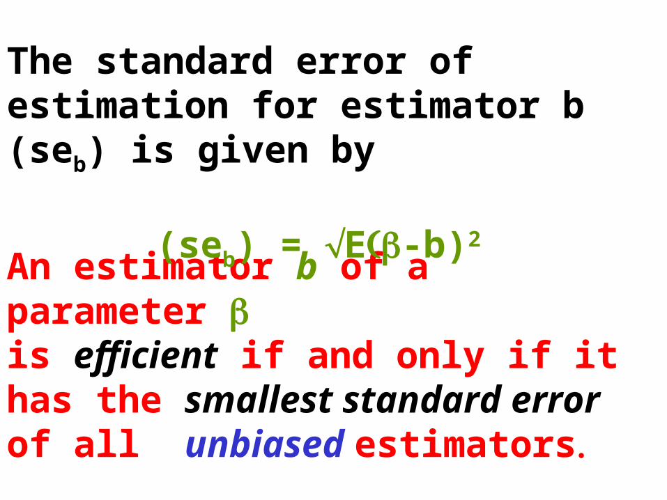
An estimator b of a parameter is efficient if and only if it has the smallest standard error of all unbiased estimators
The standard error of estimation for estimator b (seb) is given by
(seb) = E-b)2

An estimator b of a parameter is consistent if and only if its standard error gets smaller as n gets larger

Distribution of Sample Means for Various Sample Sizes
Distribution of Sample Means for Various Sample Sizes
U ShapedPopulation
n = 2 n = 5 n = 30
NormalPopulation
n = 2 n = 5 n = 30

Z Formula for Sample MeansZ Formula for Sample Means
ZX
X
n
X
X

The standard error (s.e.) of estimation for xMEAN is given by
s.e. = /n where is the population standard deviation and n is the sample size

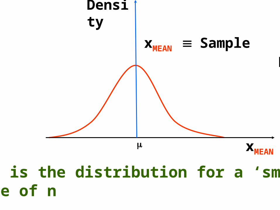
This is the distribution for a ‘small’value of n
xMEAN
xMEAN Sample Mean
Density

xMEAN
xMEAN Sample Mean
This is the distribution for a ‘small’value of n
Density
xMEAN
xMEAN Sample Mean
Density
This is the distribution for a ‘small’value of n
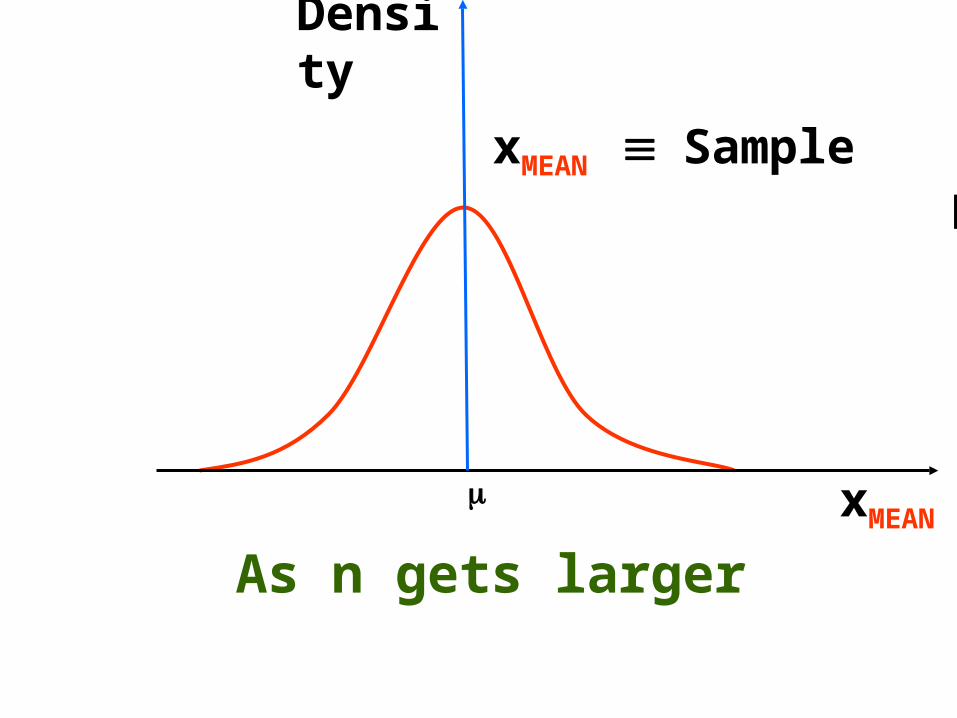
As n gets larger
xMEAN
xMEAN Sample Mean
Density

and larger….
xMEAN
xMEAN Sample Mean
Density

xMEAN
xMEAN Sample Mean
Density
and larger….

xMEAN
xMEAN Sample Mean
Density
and larger….

xMEAN
The distribution gets more compactaround the mean value (
xMEAN Sample Mean
Density
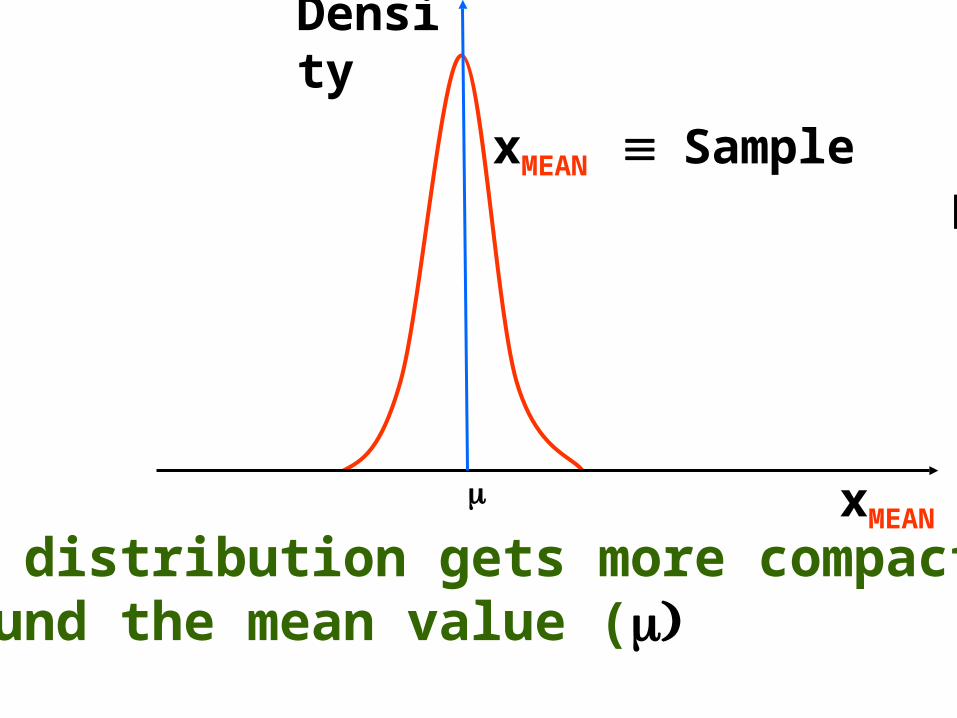
The distribution gets more compactaround the mean value (
xMEAN
xMEAN Sample Mean
Density

The distribution gets more compactaround the mean value (
xMEAN
xMEAN Sample Mean
Density

The distribution of the sample mean(xMEAN ) for three sample sizes: n1 < n2 < n3
xMEAN
Density
Sample Size: n2
Sample Size: n1
Sample Size: n3

Summary
1. XMEAN is an unbiased estimator of the population mean
E(XMEAN ) =
2. Standard error of XMEAN (s.e.) is given by s.e. = /n

3. XMEAN is an efficient estimator of the population mean . It has the smallest of all s.e values
4. XMEAN is a consistent estimator of the population mean . The s.e. value becomes smaller as the sample gets larger
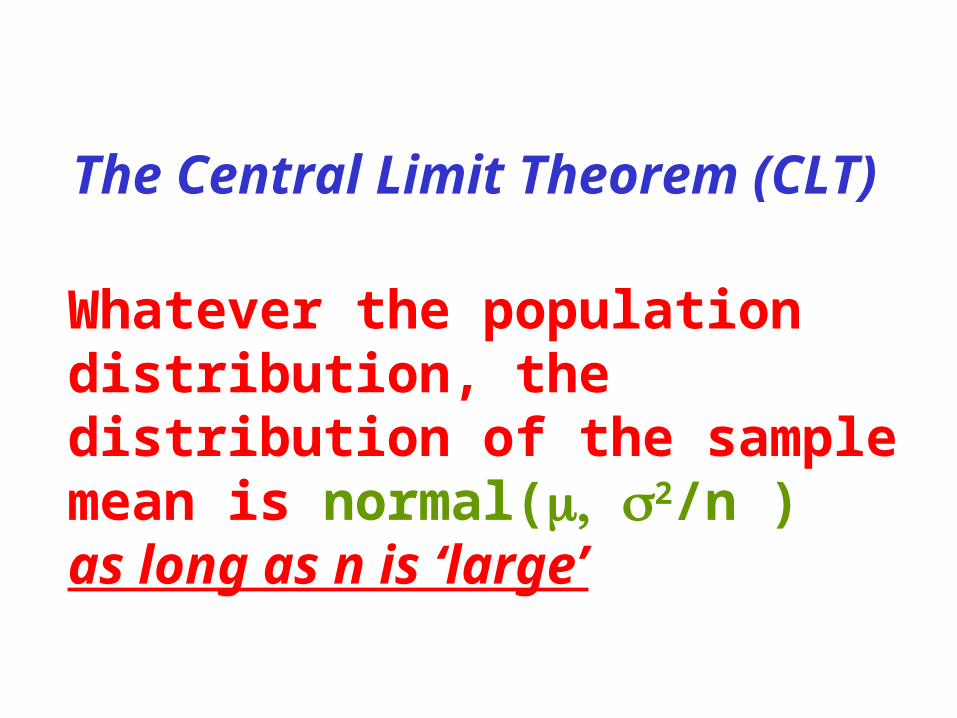
The Central Limit Theorem (CLT)
Whatever the population distribution, the distribution of the sample mean is normal( 2/n )as long as n is ‘large’

E
Frequency Density of E
.E EstimatorValue
E is an unbiased estimator

E
Frequency Density of E
.E EstimatorValue
E is a negatively biased estimator

E
Frequency Density of E
.E EstimatorValue
E is a positively biased estimator
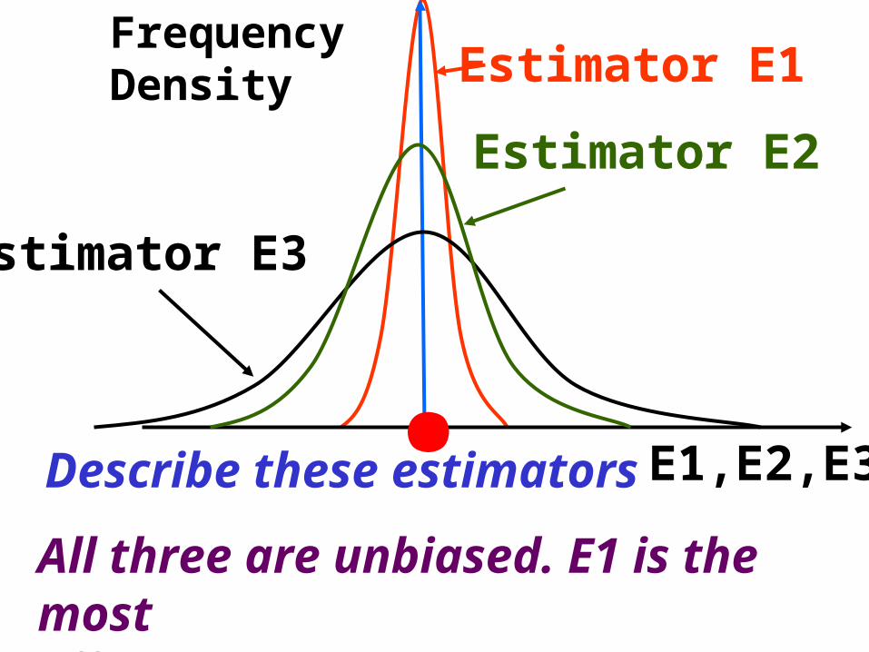
All three are unbiased. E1 is the mostEfficient, E3 is the least
FrequencyDensity
Estimator E2
Estimator E3
Estimator E1
.E1,E2,E3Describe these estimators

Both of E2 and E3 are unbiased but less efficient than E1. E1 is the most efficient, but it is positively biased.
FrequencyDensity
Estimator E2
Estimator E3
Estimator E1
.E1,E2,E3Describe these estimators

Each is a negatively biased estimator. . E1 is the most efficient of the three and E3 the least.
FrequencyDensity
Estimator E2
Estimator E3
Estimator E1
.E1,E2,E3Describe these estimators

Confidence Interval (CI)Sometimes, it is possible and
convenient to predict, with a certain amount of confidence in the prediction, that the true value of the parameter lies within a specified interval.
Such an interval is called a Confidence Interval (CI)
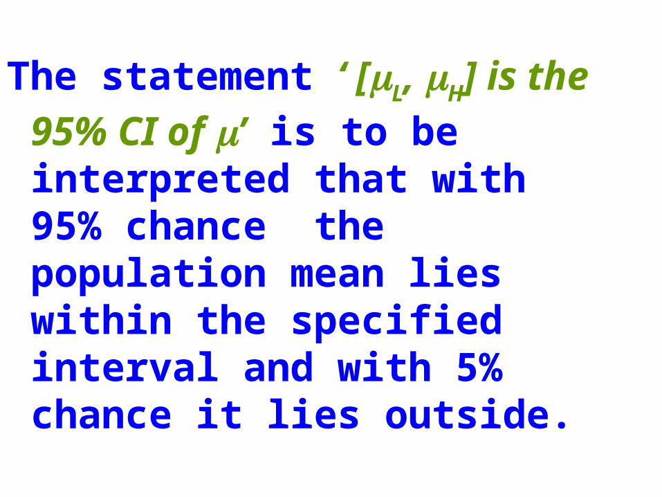
The statement ‘ [L, H] is the 95%
CI of ’ is to be interpreted that with 95% chance the population mean lies within the specified interval and with 5% chance it lies outside.
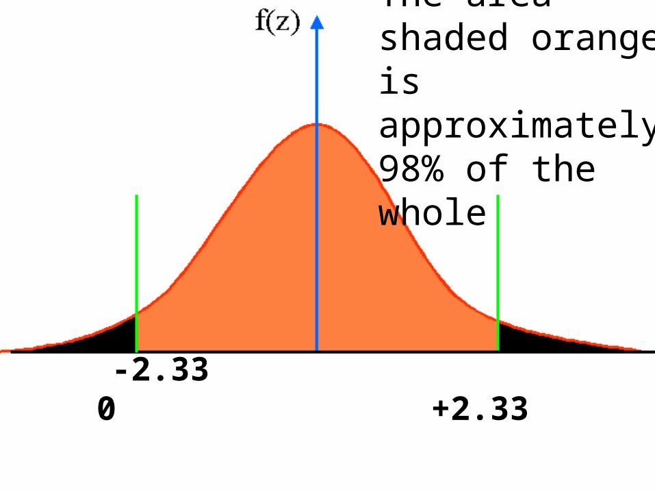
The area shaded orange is approximately98% of the whole
-2.33 0 +2.33

The area shaded orange is approximately95% of the whole
-1.96 0 +1.96

Example1 (Confidence Interval for the sample mean): Suppose that the result of sampling yields the following:
xMEAN = 25 ; n = 36. Use this information to construct a 95% CI for , given that = 16

Since n >24, we can say that xMEAN is approximately N(, 2/36).
Standardisation means that (xMEAN - )/(/6) is approximately z.
Now find the two symmetric points around 0 in the z table such that the area is 0.95. The answer is
z = 1.96.

Now solve (xMEAN - )/(6) = 1.96.
(25- )/(16/6) = 1.96 to get two values of = 19.77 and = 30.23. Thus the 95% CI for is [19.77 30.23]