Topic 1: The Regression Model - Personal WWW Pages

The Regression Model

January 12, 2012

() Applied Econometrics: Topic 1 January 12, 2012 1 / 75

Introduction

I assume you know the regression model from your 3rd year course (orother study)

I will o¤er a quick review of 3rd year material (includingheteroskedasticity and instrumental variables)

But I will also add some new material on regression including:

Maximum likelihood estimation (an estimation technique used withmost of the models to be covered in this course)

More on instrumental variables than was covered in 3rd year course

Readings: Koop (2008) chapters 2 through 5 and Gujarati chapters 1,5 and 19

You will have covered Koop (2008) chapters 2 through 5 in 3rd yearcourse (below I will highlight pages for new material)


The Regression Model

Multiple regression model with k explanatory variables:

Yi = α+ β1X1i + β2X2i + ..+ βkXki + εi

where i subscripts to denote individual observations and we havei = 1, ..,N observations.

You should know interpretation of regression coe¢ cients (asmeasuring the marginal e¤ect of an explanatory variable on adependent variable, etc.) from past study

Here I will not repeat such material, but focus on main theoreticalresults for regression model

Read Koop (2008) Chapter 2 if you want a review of how to interpretregression results


Econometric Theory of the Simple Regression Model

To keep formulae simple, use simple regression model (i.e. regressionmodel with one explanatory variable) with no intercept:

Yi = βXi + εi

where i = 1, ..,N and Xi is a scalar.

Derivations for multiple regression model are conceptually similar butformulae get complicated (use of matrix algebra usually involved)


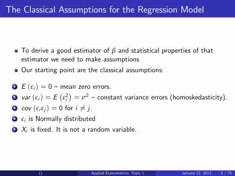
The Classical Assumptions for the Regression Model

To derive a good estimator of β and statistical properties of thatestimator we need to make assumptions

Our starting point are the classical assumptions:

1 E (εi ) = 0 �mean zero errors.2 var (εi ) = E

�ε2i�= σ2 �constant variance errors (homoskedasticity).

3 cov (εi εj ) = 0 for i 6= j .4 εi is Normally distributed5 Xi is �xed. It is not a random variable.


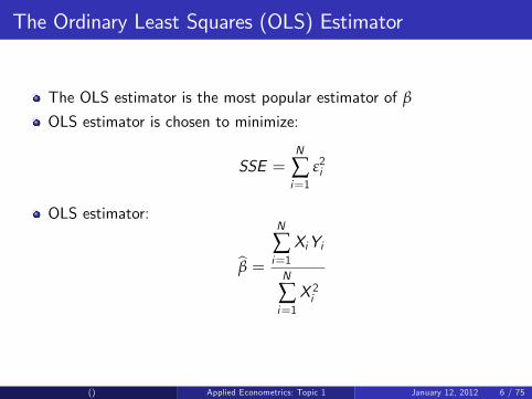
The Ordinary Least Squares (OLS) Estimator

The OLS estimator is the most popular estimator of β

OLS estimator is chosen to minimize:

SSE =N

∑i=1

ε2i

OLS estimator:

bβ =N

∑i=1XiYi

N

∑i=1X 2i


Properties of OLS Estimator under Classical Assumptions

Property 1: OLS is unbiased under the classical assumptions

E�bβ� = β

Proof of this and properties that will follow: Koop (2008), Chapter 3(or your notes for 3rd year course)


Property 2: Variance of OLS estimator under the classicalassumptions

var�bβ� = σ2

∑X 2i

Remember that variance relates to dispersion.

This property tells you how dispersed/uncertain/imprecise the OLSestimator is


Property 3: Distribution of OLS estimator under classicalassumptions bβ is N β,

σ2

∑X 2i

!Property 3 is important since we can use it to derive con�denceintervals and hypothesis tests.


Property 4: The Gauss-Markov TheoremIf the classical assumptions hold, then OLS is the best, linearunbiased estimator,

where best = minimum variance

linear = linear in y.

Short form: "OLS is BLUE"


Property 5: Under the Classical Assumptions, OLS is themaximum likelihood estimatorMaximum likelihood is another statistical principal for choosingestimators.

New material not covered in 3rd year course

Before proof, review some basic ideas in probability and introduce theidea of maximum likelihood


How do we use probability with regression model?

Assume Y is a random variable.Regression model provides description about what probable values forthe dependent variable are.Koop (2008), Chapter 2 discusses a data set and regression where Yis the price of a house and X is a size of house.What if you knew that X = 5000 square feet (a typical value in thedata set), but did not know Y ?A house with X = 5000 might sell for roughly $70, 000 or $60, 000 or$50, 000 (which are typical values in our data set), but it will not sellfor $1, 000 (far too cheap) or $1, 000, 000 (far too expensive).Econometricians use probability density functions (p.d.f.) tosummarize which are plausible and which are implausible values forthe houseNote: p.d.f.s used with continuous random variablesFor continuous random variables probabilities are area under the curvede�ned by the p.d.f.


How do we use p.d.f.s?

Figure 3.1 is example of a p.d.f.: tells you range of plausible valueswhich Y might take when X = 5, 000.Figure 3.1 a Normal distributionBell-shaped curve. The curve is highest for the most plausible valuesthat the house price might take.Remember: mean (or expected value) the "average" or "typical"value of a variableVariance is a measure of how dispersed a variable is.The exact shape of any Normal distribution depends on its mean andits variance."Y is a random variable which has a Normal p.d.f. with mean µ andvariance σ2" is written:

Y � N�µ, σ2

�() Applied Econometrics: Topic 1 January 12, 2012 13 / 75

Figure 3.1 has µ = 61.153 ! $61, 153 is the mean, or average, valuefor a house with a lot size of 5, 000 square feet.

σ2 = 683.812 (not much intuitive interpretation other than it re�ectsdispersion � range of plausible values)

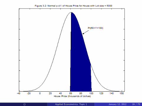
P.d.f.s measure uncertainty about a random variable since areas underthe curve de�ned by the p.d.f. are probabilities.

E.g. Figure 3.2. The area under the curve between the points 60 and100 is shaded in.

Shaded area is probability that the house is worth between $60, 000and $100, 000.This probability is 45% and can be written as:

Pr (60 � Y � 100) = 0.45

Normal probabilities can be calculated using statistical tables (oreconometrics software packages).

By de�nition, the entire area under any p.d.f. is 1.


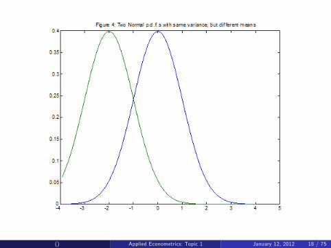
The Normal distribution is completely characterized by its mean andvariance

Di¤erent choices for µ determine the location of the Normal p.d.f.

Figure 4 plots N (0, 1) and N (�2, 1)Note p.d.f.s look same but one is shifted -2 relative to other

Di¤erent choices for σ2 determine the dispersion/spread of the p.d.f.

Figure 5 plots N (0, 1) and N (0, 4)

Note the N (0, 4) is much more dispersed/spread out than N (0, 1)


Maximum Likelihood Estimation

To derive an estimator you need to set up some criterion to optimize

For OLS you minimize the sum of squared errors (the criterion is SSE )

The maximum likelihood estimator (MLE) of β is based on a di¤erentcriterion

To motivate MLE consider return to house price example and considerFigure 3.5.

Classical assumptions imply Yi is N�

βXi , σ2�

Di¤erent values of β give di¤erent Normal distributions for Y .


Figure 3.5 plots three Normal distributions for three di¤erent choicesfor β with Xi = 5000.

β = �0.010, 0.012 and 0.040.Which one is best estimate of β?

First p.d.f. (β = �0.010): almost all of its probability to negativevalues (nonsensical, bad estimate)

Third p.d.f. (β = 0.040) allocates too much probability to very highhouse prices

Implies house price will be greater than $150, 000 (out of line withobservations in this data set)

Second p.d.f. (β = 0.012) is same as Figure 3.1

Much more sensible (house price of house with lot size of 5, 000probably around $60,000 which is type of value observed in data set).

β = 0.012 is most likely estimate �maximum likelihood estimator


Formal De�nition of Maximum Likelihood

P.d.f. of one observation: p (Yi jXi , β)If observations are independent of one another, then joint p.d.f. allthe observations can be written as:

p (Y1, ..,YN ) =N

∏i=1p (Yi jXi , β)

Plug in the observed data in p (Y1, ..,YN ) then the only thing leftunknown is β so call this joint p.d.f. (with actual data plugged in)L (β)L (β) is called the likelihood functionMaximum likelihood estimation: choose value for β which maximizesL (β).Note: the idea of maximum likelihood can be used with any model,not just the regression modelGretl uses maximum likelihood estimation for many of the modelsdiscussed later in this course


Maximum Likelihood Estimation in the Regression Model

Property 5: The maximum likelihood estimator of β is the OLSestimator (under the classical assumptions)

Proof: Using the formula for the Normal p.d.f. (see Appendix B,De�nition B.10), we obtain:

p (Yi jXi , β) =1p2πσ2

exp�� 12σ2

(Yi � βXi )2�

The likelihood function is product of this p.d.f. over everyobservation.


Using the properties of the exponential function, this can becalculated as:

L (β) =N

∏i=1

1p2πσ2

exp�� 12σ2

(Yi � βXi )2�

=1

(2πσ2)N2

exp

"� 12σ2

N

∑i=1(Yi � βXi )

2

#

=1

(2πσ2)N2

exp��SSE2σ2

�Finding MLE is a straightforward calculus problem: �nd value for βwhich maximizes L (β)


I won�t do derivation, but (if you know properties of exp function) youcan see the answer:

How to make L (β) as large as possible? Make SSE as small aspossible

Need to minimize SSE � but this is exactly what OLS does

In regression model MLE and OLS are exactly the same

In other models used in this course, we will often use MLEs

Sometimes impossible to analytically work out MLE �need numericaloptimization procedures

Gretl will do this for you


Using Information Criteria to Select a Model

While I am discussing MLE, digress to introduce the idea ofinformation criterion

Often researcher wants to choose between several models (e.g. twomodels with di¤erent explanatory variables)

Information criteria can be used to do this (for any set of modelswhich seek to explain the same dependent variable)

Information criterion can be used for regression, probit, logit, countdata, etc. etc.

To use an information criteria, you simply calculate it for every modeland select the model which yields the lowest information criterion

Very simple to use and can be used with all the models in this course(not just regression)


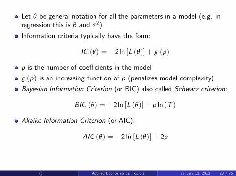
Let θ be general notation for all the parameters in a model (e.g. inregression this is β and σ2)

Information criteria typically have the form:

IC (θ) = �2 ln [L (θ)] + g (p)

p is the number of coe¢ cients in the model

g (p) is an increasing function of p (penalizes model complexity)

Bayesian Information Criterion (or BIC) also called Schwarz criterion:

BIC (θ) = �2 ln [L (θ)] + p ln (T )

Akaike Information Criterion (or AIC):

AIC (θ) = �2 ln [L (θ)] + 2p


Estimation of Sigma-squared

Remember: Residuals are:

bεi = Yi � bβXiAn unbiased estimator of σ2 is

s2 =∑bε2iN � 1

Property (not proved in this course):

E�s2�= σ2

Note: The N � 1 in denominator becomes N � k � 1 in multipleregression where k is number of explanatory variables.


Con�dence Intervals and Hypothesis Testing

Con�dence intervals provide interval estimates

Give a range in which you are highly con�dent that β must lie.

Basic idea in testing any hypothesis, H0:

�The econometrician accepts H0 if the calculated value of the teststatistic is consistent with what could plausibly happen if H0 is true.�

�Level of signi�cance� (usually 5%) formalizes �what could plausiblyhappen�

Test statistic compared to �critical value�which is a formal check ofthe �is consistent with�part of the previous sentence

The t-statistic is used to test H0:β = 0

F-statistics used to test more complicated hypotheses involving morethan one coe¢ cient in multiple regression


Note on P-values

All relevant computer packages present P-values for many hypothesistests. This means you do not need to look up critical values instatistical tables.

Useful (but not quite correct) intuition: "P-value is the probabilitythat H0 is true"

A correct interpretation: "P-value equals the smallest level ofsigni�cance at which you can reject H0"

Example: If P-value is .04 you can reject H0 at 5% level ofsigni�cance or 10% or 20% (or any number above 4%). You cannotreject H0 at 1% level of signi�cance.

Common rule of thumb:

Reject H0 if P-value less than .05.


Violations of the Classical Assumptions

Previous results all derived using classical assumptions

What if classical assumptions are violated?

Need to �nd out if this is so (need hypothesis tests) and, if so, useestimators other than OLS

Chapter 5 of Koop (2008) �covered in 3rd year course � wentthrough violations of classical assumptions

Here we do:

Quick review of heteroskedasticity with more emphasis onheteroskedasticity consistent estimation (HCE)

Note: HCE can be done in Gretl (but not Excel)

Instrumental variable (IV) estimation (more detail than in 3rd yearcourse)


Heteroskedasticity

Heteroskedasticity relates to Assumption 2.

Basic ideas:

Under classical assumptions, Gauss Markov theorem says "OLS isBLUE". But if Assumption 2 is violated OLS this no longer holds(OLS is still unbiased, but is no longer "best". i.e. no longerminimum variance).

If heteroskedasticity is present, you should use either GeneralizedLeast Squares (GLS) estimator or HCE


Heteroskedasticity occurs when the error variance di¤ers acrossobservations

Here is the story I told in 3rd year course relating to house price dataset:

Errors re�ects mis-pricing of houses

If a house sells for much more (or less) than comparable houses, thenit will have a big error

Error variance measures the dispersion of errors/degree of possiblemis-pricing houses

Suppose small houses all very similar, then unlikely to be large pricingerrors

Suppose big houses can be very di¤erent than one another, thenpossible to have large pricing errors

If this story is true, then expect errors for big houses to have largervariance than for small houses

Statistically: heteroskedasticity is present and is associated with thesize of the house


Assumption 2 replaced by var (εi ) = σ2ω2i for i = 1, ..,N.

Note: ωi varies with i so error variance di¤ers across observations

GLS proceeds by transforming model and then using OLS ontransformed model

Transformation comes down to dividing all observations by ωi

Problem with GLS: in practice, it can be hard to �gure out what ωi is

To do GLS need to �nd answer to questions like:

Is ωi proportional to an explanatory variable? If yes, then which one?

Can be hard to do.


Thus HCEs are popular

Use OLS estimates, but corrects its variance (var�bβ�) so as to get

correct con�dence intervals, hypothesis tests, etc.

They can be automatically calculated in Gretl

Advantages: HCEs are easy to calculate and you do not need to knowthe form that the heteroskedasticity takes.

Disadvantages: HCEs are not as e¢ cient as the GLS estimator (i.e.they will have larger variance).


Testing for Heteroskedasticity

If heteroskedasticity is NOT present, then OLS is �ne (it is BLUE).

But if it is present, you should use GLS or a HCE

Thus, it is important to know if heteroskedasticity is present.

There are many tests, here I will describe two of the most popularones: the White test and the Breusch Pagan test

These are done in Gretl


Breusch-Pagan Test for Heteroskedasticity

Suppose you think the error variance might depend on any or all ofthe variables Z1, ..,Zp (which may be the same as the explanatoryvariables in the regression itself).

Breusch-Pagan test involves the following steps:


Run OLS on the original regression (ignoring heteroskedasticity) andobtain the residuals, bεi , and using the residuals calculate:

bσ2 = ∑bε2iN

Run a second regression of the equation:

bε2ibσ2 = γ0 + γ1Z1i + ..+ γpZpi + vi

Calculate the Breusch-Pagan test statistic using the regression sum ofsquares (RSS) from this second regression:

BP =RSS2

This test statistic has a χ2 (p) distribution, which can be used to geta critical value from.


The White Test for Heteroskedasticity

Similar to the Breusch-Pagan test

White test involves the following steps:


Run OLS on the original regression (ignoring heteroskedasticity) andobtain the residuals, bεi .Run a second regression of the equation:

bε2i = γ0 + γ1Z1i + ..+ γpZpi + vi

and obtain the R2 from this regression.

Calculate the White test statistic:

W = NR2

This test statistic has a χ2 (p) distribution which can be used to geta critical value from.

Note: in the pure White test, Z1, ..,Zp incude the explanatoryvariables in the regression plus squares and cross-products of them


Instrumental Variable Methods

Overview: Under the classical assumptions, OLS is BLUE.

When we relax Assumptions 2 or 3 (e.g. to allow forheteroskedasticity or autocorrelated errors), then OLS is no longerBLUE but it is still unbiased (although GLS is better)

However, in the case we are about to consider, OLS will be biasedand an entirely di¤erent estimator will be called for �the instrumentalvariables (IV) estimator.

Here we relax assumption that explanatory variables are not randomvariables.

For simplicity, use simple regression model, but results generalize tothe case of multiple regression.

Some of this material was covered in 3rd year course, but there ismuch that is new


Theory Motivating the IV Estimator

Reminder of basic theoretical results

Previously derived theoretical results using multiple regression modelwith classical assumptions:

1 E (εi ) = 0 �mean zero errors.2 var (εi ) = E

�ε2i�= σ2 �constant variance errors (homoskedasticity).

3 cov (εi εj ) = 0 for i 6= j .4 εi is Normally distributed5 Explanatory variables are �xed. They are not random variables.


Case 1: Explanatory Variable is Random But isUncorrelated with Error

Now relax classical Assumption 5 and assume Xi is a random variable,

We have to make some assumptions about its distribution.

Assume Xi are independent and identically distributed (i.i.d.) randomvariables with:

E (Xi ) = µXvar (Xi ) = σ2X

In Case 1 we will assume explanatory variable and errors areuncorrelated with one another:

cov (Xi , εi ) = E (Xi εi ) = 0


Remember, under classical assumptions:

bβ is N β,σ2

∑X 2i

!

This result can still be shown to hold approximately in this case (I willnot provide details, some given in textbook)

Bottom line: If we relax the assumptions of Normality and �xedexplanatory variables we get exactly the same results as for OLSunder the classical assumptions (but here they hold approximately),provided explanatory variables are uncorrelated with the error term.


Case 2: Explanatory Variable is Correlated with the ErrorTerm

Assume Xi are i.i.d. random variables with:

E (Xi ) = µXvar (Xi ) = σ2X

In Case 2 we will assume explanatory variable and errors arecorrelated with one another:

cov (Xi , εi ) = E (Xi εi ) 6= 0

It turns out that, in this case, OLS is biased and a new estimator iscalled for: the instrumental variables (IV) estimator.

See Koop (2008) page 152 (or your notes for 3rd year course)


The Instrumental Variables Estimator

An instrumental variable (IV), Zi , is a random variable which isuncorrelated with the error but is correlated with the explanatoryvariable.Formally, an instrumental variable is assumed to satisfy the followingassumptions:

E (Zi ) = µZvar (Zi ) = σ2Zcov (Zi , εi ) = E (Zi εi ) = 0cov (Xi ,Zi ) = E (XiZi )� µZµX = σXZ 6= 0

Assuming an instrumental variable exists (something we will return tolater), IV estimator:

bβIV =N

∑i=1ZiYi

N

∑i=1XiZi


Can show (approximately):

bβIV is N

β,

�σ2Z + µ2Z

�σ2

N (σXZ + µX µZ )2

!

Note: this implies E�bβIV � = β so unbiased (approximately)

This formula can be used to calculate con�dence intervals, hypothesistests, etc. (comparable to Topic 3 slide derivations)

In practice, the unknown means and variances can be replaced bytheir sample counterparts.

Thus, µX can be replaced by X , σ2Z by the sample variance of(Zi�Z )

2

N�1 , etc.

No additional details of how this is done, but note that econometricssoftware packages do IV estimation.

Note: this is sometimes called the two stage least squares estimator(and Gretl uses this term)


Using the IV Estimator in Practice

what if you have a multiple regression model involving more than oneexplanatory variable?

Answer: you need at least one instrumental variable for eachexplanatory variable that is correlated with the error.

Note: if even only one of the explanatory variables in a multipleregression model is correlated with the errors, OLS estimates of allcoe¢ cients can be biased.

what if you have more instrumental variables than you need?

Use the generalized instrumental variables estimator (GIVE).


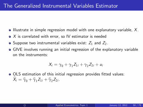
The Generalized Instrumental Variables Estimator

Illustrate in simple regression model with one explanatory variable, X .

X is correlated with error, so IV estimator is needed

Suppose two instrumental variables exist: Z1 and Z2.

GIVE involves running an initial regression of the explanatory variableon the instruments:

Xi = γ0 + γ1Z1i + γ2Z2i + ui

OLS estimation of this initial regression provides �tted values:bXi = bγ0 + bγ1Z1i + bγ2Z2i .


It can be shown that bX is uncorrelated with the errors in the originalregression and, hence, that it is a suitable instrument.

This is what GIVE uses as an instrument.

Thus, the GIVE is given by:

bβGIVE =N

∑i=1

bXiYiN

∑i=1Xi bXi


The Hausman Test

Hausman test used to see if IV estimator is necessary

If X correlated with error, then OLS is biased and you should use anIV estimator.

However, if X uncorrelated with error, then (under the classicalassumptions) OLS is BLUE and, hence, is more e¢ cient than IV.

Basic idea of Hasuman test (Gretl will calculate it for you):

Let H0 be the hypothesis that explanatory variables are uncorrelatedwith error.

If H0 is true, then both OLS and IV are both acceptable estimatorsand should give roughly the same result.

However, if H0 is false, then OLS in not acceptable, but IV is andthey can be quite di¤erent.

Hausman test based measuring the di¤erence between bβ and bβIV .() Applied Econometrics: Topic 1 January 12, 2012 52 / 75

It can be shown that Hausman test can be done using OLS methods

Example: simple regression with one instrument.

Original regression model of interest is:

Yi = α+ βXi + εi

Hausman test uses this regression but adds the instrumental variableto it:

Yi = α+ βXi + γZi + εi

Can be shown that Hausman test is equivalent to t-test of H0 : γ = 0.

If coe¢ cient on Z is signi�cant, you reject H0 and use the IVestimator.

If coe¢ cient on Z is insigni�cant, do OLS on original regression model


Example: Hausman test in multiple regression model

Suppose we have 3 explanatory variables (X1,X2 and X3), 2 of whichmight be correlated with the error (X2 and X3).

For X2 we have two possible instrumental variables (Z1 and Z2),

For X3 we have three possible instrumental variables (Z3,Z4 and Z5)

Since potentially more instruments than explanatory variables, mightwant to use GIVE

Hausman test runs initial GIVE regressions (see the discussion of theGIVE) to get �tted values, bX2 and bX3Then add these �tted values to original regression and tests if theyare signi�cant

Precise steps given on next slide


Run an OLS regression of X2 on an intercept, Z1 and Z2. Obtain the�tted values, bX2.Run an OLS regression of X3 on an intercept Z3,Z4 and Z5. Obtainthe �tted values, bX3.Run an OLS regression of Y on an intercept X1,X2,X3, bX2 and bX3.Do an F-test of the hypothesis that the coe¢ cients on bX2 and bX3 arejointly equal to zero.

If the F-test rejects, then proceed with GIVE, if not use OLS on theoriginal regression.


The Sargan Test

Hausman test tells you whether it is necessary to do instrumentalvariables estimation, if we have valid instrumental variables

But how do we know that Z truly is a valid instrument?

Remember to be a valid instrument, Z must be correlated with X butuncorrelated with regression error.

The latter is not easy to check, since the regression error is notobserved.

The issue of testing whether instruments truly are valid ones isdi¢ cult

If you have only one potential instrument for every explanatoryvariable, there is no way of testing instrument validity

Next slide illustrates why this is so


Suppose one potential instrument, Z for a simple regression model:

Yi = βXi + εi

For Z to be instrument must have cov (Zi , εi ) = 0.

εi is unobserved, but why not create a test statistic based oncov (Zi ,bεi ) using residualsBut which residuals should you use?

IV residuals (i.e. bεIVi = Yi � bβIVXi ) sound plausible, but will beunacceptable if Z is not a valid instrument

OLS residuals are inappropriate since they could very well be biased(and you cannot use a Hausman test to check this, since you are notsure that Z is a valid instrument).

In fact, there is no way of testing whether the instruments are valid insuch a case.


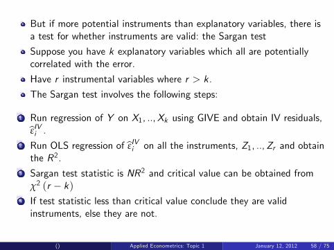
But if more potential instruments than explanatory variables, there isa test for whether instruments are valid: the Sargan test

Suppose you have k explanatory variables which all are potentiallycorrelated with the error.

Have r instrumental variables where r > k.

The Sargan test involves the following steps:

1 Run regression of Y on X1, ..,Xk using GIVE and obtain IV residuals,bεIVi .2 Run OLS regression of bεIVi on all the instruments, Z1, ..,Zr and obtainthe R2.

3 Sargan test statistic is NR2 and critical value can be obtained fromχ2 (r � k)

4 If test statistic less than critical value conclude they are validinstruments, else they are not.


Why Might the Explanatory Variable Be Correlated withError?

There are many di¤erent reasons why the explanatory variables mightbe correlated with the errors.

Errors in Variables problem (covered in 3rd year course, not repeatedhere. see Koop, 2008, page 158)

Returns to schooling example (covered in 3rd year course, brie�yrepeated here,see Koop, 2008, pages 162-163)

Simultaneous equations model (new material given here)


The Simultaneous Equations Model

Example: supply and demand model

Demand curve:QD = βDP + εD

Supply curveQS = βSP + εS

QD is quantity demanded, QS is quantity supplied, P is price

In equilibrium, QD = QS and this condition is used to solve forequilibrium price and quantity.

Price and quantity are determined by this model so they are bothendogenous variables.

These two equations are a simultaneous equations model.


Suppose econometrician collects data on price and quantity and runsa regression of quantity on price.

This will yield an estimate � β.

But would it be an estimate of βD or βS?

There is no way of knowing.

OLS will probably neither estimate the supply curve nor estimate thedemand curve.


How might we solve this problem?

Include exogenous variable (not determined by the model).

E.g. suppose QD depends also on the income, I :

QD = βDP + γI + εD

Notation: original supply and demand model is structural form.

When we solve model so that only exogenous variables on right handside, we get reduced form


Setting QD = QS and solving for equilibrium P and QSet right-hand sides of the demand and supply equations equal toeach other, and rearrange:

P =�γ

βD � βSI +

εS � εDβD � βS

= π1I + ε1

Substitute this expression for P into the supply equation:

Q = βS (π1I + ε1) + εS

= βSπ1I + βS ε1 + εS

= π2I + ε2

Note: I am using π1 =�γ

βD�βSand π2 = βSπ1 as notation for

reduced form coe¢ cientsε1 and ε2 are reduced form errors which are functions of the structuralform errorsThis example shows what reduced and structural form are, but whatare the implications for the econometrics?


Directly Estimating Structural Equations using OLS Leadsto Biased Estimates

Why not run a regression based on the demand curve?

Regression of Q on P and I?

Can show explanatory variable P is correlated with the error.

As shown in this section of lecture slides, OLS is not appropriate

To prove this, assume εS and εD are uncorrelated and homoskedastic

var (εD ) = σ2Dvar (εS ) = σ2SAssume exogenous variable I is not random


cov (P, εD ) = E (PεD )

= E [(π1I + ε1) εD ]

= E��

εS � εDβD � βS

�εD

�=

�σ2DβD � βS

6= 0,


OLS Estimation of Reduced Form Equations is Fine

It is not hard to show that reduced form errors do satisfy the classicalassumptions.

Thus, OLS estimation of reduced form equations is BLUE

So bπ1 and bπ2 are BLUE, but what are they estimates of?For instance, π1 =

�γβD�βS

which is not the slope of supply curve ordemand curve.

But here we can estimate slope of supply curve using bπ1 and bπ2We have

π2 = βSπ1

and, thus, bβS = bπ2bπ1Such a strategy is called indirect least squares.


How does all this relate to instrumental variables?

Easy to show that indirect least squares is equivalent to instrumentalvariable estimation of supply curve using I as an instrument

This example sheds insight on how to choose instruments

Note: here we are estimating the supply curve, but there is no way ofestimating the demand curve

Why is this?

Key thing is that income does not appear in supply curve.

A general rule is: if you have an exogenous variable which is excludedfrom an equation, then it can be used as an instrumental variable forthat equation.

This occurs for supply curve, but not demand curve


An example where the explanatory variable could becorrelated with the error

Suppose interested in estimating returns to schooling and have datafrom a survey of many individuals on:

The dependent variable: Y = income

The explanatory variable: X = years of schooling

And other explanatory variables like experience, age, occupation, etc..which we will ignore here to simplify exposition.

My contention is that, in such a regression it probably is the case thatX is correlated with the error and, thus, OLS will be inappropriate.


To understand why, �rst think of how errors are interpreted in thisregression.

An individual with a positive error is earning an unusually high level ofincome. That is, his/her income is more than his/her education wouldsuggest.

An individual with a negative error is earning an unusually low level ofincome. That is, his/her income is less than his/her education wouldsuggest.

What might be correlated with this error?

Perhaps each individual has some underlying quality (e.g. intelligence,ambition, drive, talent, luck �or even family encouragement).


This quality would like be associated with the error (e.g. individualswith more drive tend to achieve unusually high incomes).

But this quality would also e¤ect the schooling choice of theindividual. For instance, ambitious students would be more likely togo to university.

Summary: Ambitious, intelligent, driven individuals would both tendto have more schooling and more income (i.e. positive errors).

So both the error and the explanatory variable would be in�uenced bythis quality.

Error and explanatory variable probably would be correlated with oneanother.


How do you choose instrumental variables?

There is a lot of discussion in the literature how to do this. But this istoo extensive and complicated for this course, so we o¤er a fewpractical thoughts.

An instrumental variable should be correlated with explanatoryvariable, but not with error.

Sometimes economic theory (or common sense) suggests variableswith this property.

In our example, we want a variable which is correlated with theschooling decision, but is unrelated to error (i.e. factors which mightexplain why individuals have unusually high/low incomes)

An alternative way of saying this: we want to �nd a variable whicha¤ects schooling choice, but has no direct e¤ect on income.


Characteristics of parents or older siblings have been used asinstruments.

Justi�cation: if either of your parents had a university degree, thenyou probably come from a family where education is valued (increasethe chances you go to university). However, your employer will notcare that your parents went to university (so no direct e¤ect on yourincome).

Other researchers have used geographical location variables asinstruments.

Justi�cation: if you live in a community where a university/college isyou are more likely to go to university. However, your employer willnot care where you lived so location variable will have no direct e¤ecton your income.


Summary

This set of slides reviews regression model (and adds some newmaterial)

Under classical assumptions OLS is BLUE

Con�dence intervals are interval estimates

Hypothesis testing was reviewed

Maximum likelihood estimation introduced

Latter half of these slides relate to violations of classical assumptions


If errors either have di¤erent variances (heteroskedasticity) or arecorrelated with one another, then OLS is unbiased, but is no longerthe best estimator. The best estimator is GLS.If heteroskedasticity is present, then the GLS estimator can becalculated using OLS on a transformed model. If suitabletransformation cannot be found, then heteroskedasticity consistentestimator should be used.There are many tests for heteroskedasticity, including theBreusch-Pagan and the White test.In many applications, it is implausible to treat the explanatoryvariables and �xed. Hence, it is important to allow for them to berandom variables.If explanatory variables are random and all of them are uncorrelatedwith the regression error, then standard methods associated with OLSstill work.If explanatory variables are random and some of them are correlatedwith the regression error, then OLS is biased. The instrumentalvariables estimator is not.


In multiple regression, at least one instrument is required for everyexplanatory variable which is correlated with the error.

If you have valid instruments, then the Hausman test can be used totest if the explanatory variables are correlated with the error.

In general, cannot test whether an instrumental variable is a validone. However, if you have more instruments than the minimumrequired, the Sargan test can be used.

Explanatory variables can be correlated with error they are measuredwith error.

Explanatory variables can be correlated with the error in thesimultaneous equations model


Topic 1: The Regression Model - Personal WWW Pages

Documents

Transcript of Topic 1: The Regression Model - Personal WWW Pages