1

I~EC ii

VOL. 6 NO.4 OCTOBER 1967

lEPDAW

INDUSTRIAL & ENGINEERINGCHEMISTRY

PROCESS DESIGNAND DEVELOPMENT

Pilot-Plant Development of Foam DistributionProcess for Production of Wet-Process Phos-phoric Acid

G. G. Patterson, J. R. Gahan, and W. C. Scott

Rate of Sulfur Dissolution in Aqueous SodiumSulfide

Nils Hartler, Jan Libert, and Ants Teder . . . . .

Reaction of Sulfur Oxides with Phosphate RockL. W. Ross and H. C. Lewis . . . . . . . . . .

/Fluidized Bed Disposal of FluorineJ. T. Holmes, L. B. Koppel, and A. A. Jonke .

Polyphosphates by Selective Extraction of Super-phosphoric Acids

C. Y. Shen .

Ion Exchange Treatment of Mixed Electroplat-ing Wastes

J. A. Tallmadge . . . . . . . . . . . . . .

Concentration and Separation of Ions by DonnanMembrane Equilibrium

R. M. Wallace . . . . . . . . . . . . . . .

Role of Slurry Particle Geometry and State ofAggregation in Changing Kinetics of a React-ing Slurry System. Acetylation of AlkylChlorides with Sodium Acetate

Leon Polinski and I-Der Huang . . . . . . . .

Oxidation of Methane to Formaldehyde in aFluidized Bed Reactor

B. H. McConkey and P. R. Wilkinson . . . . .

/,Quality of Control Problem for Dead-Time Plants/' T. J. McAvoy and E. F. Johnson . . . . . . . .

.. ' Linear Temperature Control in Batch Reactors, M. C. Millman and Stanley Katz . . . . . . .

/ Time-Optimum Control of Chemical Processesfor Set-Point Changes

P. R. Latour, L. B. Koppel, and D. R. Coughanowr

/" Noninteracting Process ControlShean-lin Liu . . . . . . . . . . . . . . . .

393 Batch Heat Transfer Coefficients for~PseudoplasticFluids in Agitated Vessels

Donald Hagedorn and J. J. Salamone . . . . . .

460

398 Multiple Automated MicrounitsC. D. Ackerman, A. B. Hartman, and R. A. Wright

469

476

480

486

499

504

516

525

532

535

539

407 Design of Air Pulsers for Pulse Column Applica-tion

M. E. Weech and B. E. Knight ...

408 Cocurrent Gas-Liquid ContactingColumns

L. P. Reiss .

in Packed

414 Calculation of Effect of Vapor Mixing on TrayEfficiency

D. A. Diener . . . . . . . . . . . . . . . .

419 Correlations of Reverse Osmosis Separation Datafor the System Glycerol-Water Using PorousCellulose Acetate Membranes

S. Sourirajan and Shoji Kimura. . . . . . . . .423

Adsorption of Normal Paraffins from BinaryLiquid Solutions by SA Molecular SieveAdsorbent

P. V. Roberts and Robert York. . . . . . .

432 Froth and Foam Height Studies. Small Perfor-ated Plate Distillation Column

D. A. Redwine, E. M. Flint, and Matthew Van Winkle

436 Simulation of Heat-Transfer Phenomena in c.IRotary Kiln

Allan Sass . .440

CORRESPONDENCE447 /Optimal Adiabatic Bed Reactor with Cold Shot

CoolingJ.-P. Malenge and Jacques Villermaux .

Index.452

TIME-OPTIMUM CONTROL OF CHEMICALPROCESSES FOR SET-POINT'CHANGES

School of Chemical Engineering, Purdue University, J17estLafayette, Ind.

PIERRE R. LATOUR,! LOWELL B. KOPPEL, AND DONALD R. COUGHANOWR

A procedure to drive the process output to a new operating level in minimum time is proposed for a wide class

of single-manipulated-input, single-output processes subject to input saturation. The bang-bang control

based upon switching times can be implemented in a programmed sense either manually or with direct

digital control for set-point changes without detailed process dynamics information. A technique for fitting

the model to bang-bang response data allows possible adaptation.

INCREASING competition and technology in the process in-dustries provide economic incentive for optimization.

Supervisory digital control is a proved and widely used con-cept for commercial plants (Crowther et al., 1961; Williams,1965). Typical operation is as follows: A digital computerperforms a steady-state optimization perhaps hourly based oncurrent operating conditions. Each optimization results in anew set of set-point values for the plant loops. The computermakes the required step changes in set points of the conven-tional controllers, which must therefore be adjusted for acompromise between good set-point and load responses.The results given in the present paper provide an improved,practical technique for achieving good set-point responses,while allowing the conventional controllers to be tuned forgood regulator action so that load disturbances will be wellcompensated. This will significantly improve the performanceof such supervisory control systems.

Criterion of Optimality

For commercial processes, maximum return on investmentor profit is perhaps the most common criterion function foroptimum engineering design. Since the economic criterionfunctions are unique to each problem, and may be difficult tostate or use mathematically, we propose a minimum timecriterion as a useful general criterion of optimality for the servoproblem in process control. The reasons for this choice are:A particularly simple implementation results, the responseswhich are achieved will generally provide significant improve-ment over conventional controller set-point responses by anycriterion of optimality, and the process dynamics are onlyinfrequently known to sufficient accuracy to warrant use of amore complex criterion function.

Bang-Bang Control

Intuitively one feels that the harder a system is forced thefaster it will respond. However, there is always a physicallimit to the available energy for control. Saturation occursin an automatic valve when it is wide open or closed tight.The resulting limits on the available energy must be consideredand utilized in forcing the system as rapidly as possible,This constraint on the manipulated variable will be writtenas k :::; m(t) :::; K.. In conventional regulator design methods,error perturbations are assumed to be small, and linear theoryis applied to design linear controllers. Although errors arekept small during the design calculations to avoid saturationdeliberately and ensure that linearity is preserved, such con-

i Present address, Shell Oil Co., Houston, Tex.

452 1& E CPR 0 C E S S DES I G NAN D D EVE lOP MEN T

trollers do not take proper account of the saturation whichinevitably occurs in operation.

From Pontryagin's maximum principle (Pontryagin et al.,1962), Gibson and Johnson (1963) have shown that the time-optimum control action for linear processes, subject to satura-tion on m(t), requires the manipulated variable to be at thebounds of its limits throughout the transient-that is, m(t) willbe at either k or K, with possible switches between thesevalues, during the entire transient. Such nonlinear controlaction is called extremal or bang-bang control.

It is understood that if driving the process with m(t) at itsactual physical constraint can cause mechanical damage orundesirable conditions in the system, a less severe pseudo-constraint may be assumed, at the expense of response time,of course-that is, the values of k and K. need not representtrue physical limits, and in practice would be assigned con-servative values initially until the controller tests were com-pleted.

Also we assume m can be switched instantaneously betweenK. and k. This is not a severe restriction if valve dynamicsare lumped with the process.

Mathematical ModelRational design of a process controller requires some sort of

mathematical description of the process dynamics. Absoluteoptimum control of a physical process can seldom be achieved;only optimum control of its mathematical model is possible.Obviously, if the model is a good mirror of reality, the controldesigned to be optimum on the model will approach the trueoptimum for the physical process. A comparison betweenthe open-loop responses of the model and process is only anindirect measure of the model's validity. A direct measureis the performance of the resulting controller when it is appliedto the physical system.

Synthesis of a mathematical model for process dynamics, asin statistical regression, requires determination of both themodel form and the model parameters. Lefkowitz (1963)has stated that the model complexity and the analysis pro-cedure used are highly dependent upon the purpose intendedfor the model. For process scale-up and extrapolation,complex models based upon fundamental laws of physicsand chemistry are usually required. However, for inter-polation and for many control system designs, simpler empiricalmodels with statistically fitted parameters may suffice. Com-plex theoretical models are avoided here for the followingreasons:

Process dynamics arc neither well known nor susceptible toaccurate measurement.

Rigorous models tend to contain nonlinearities and distrib-uted parameters.

Control theory is not well developed for such models andeach design tends to be unique to its process.

Rigorous models have many parameters that are unknown ordifficult to measure. Few state variables can be measureddirectly for feedback, so higher-order models are of limitedutility even if the process dynamics are theoretically of highorder. Also, optimal control algorithms for higher-ordermodels have not been obtained from present-day theory.

Detailed process analyses and complex controllers aredifficult to justify economically for most single-manipulated-input single-output processes, because we will show that signif-icant control improvement can often be achieved based onsimpler process dynamics models.

For these reasons, an overdamped second-order model withdead time and fitted parameters is assumed to describe theprocess dynamics to sufficient accuracy that the optimumcontroller for this model performs significantly better than aconventional one, on the actual process. Note the significantdifference between this statement and the statement that thedynamic response of the process may be described to somespecified level of accuracy by that of the model. The transferfunction of this model is

C(s)M(s)

Kp(aTs + 1)exp( -dTs)(Ts+ 1)(bTs+ 1)

where

C process output to be controlled}J manipulated variableKp = process gain, units e/mT major time constantb T minor time constant, ° S b S 1dT dead time, d ;:::0aT numerator time constant

This model can be used to represent the dynamic responseof liquid-liquid and gas-liquid extractors (Biery and Boylan,1963; Gray and Prados, 1963), mixing in agitated vessels(Marr and Johnson, 1961), some heat exchangers (Hougen,1963), distillation columns (Lupfer and Parsons, 1962; Moczecket al., 1965; Sproul and Gerster, 1963), and some chemicalreactors (Lapse, 1956; Lupfer and Oglesby, 1962; Mayerand Rippel, 1963; Roquemore and Eddey, 1961). Clearly,however, there exist processes which cannot usefully bedescribed by such dynamics, and the specific results of thispaper are not directly applicable to such processes, althoughthe general methods may be applicable with more mathe-matical effort. We will nevertheless demonstrate that even anonlinear exothermic chemical reactor may sometimes beusefully treated by using Equation 1 for a model.

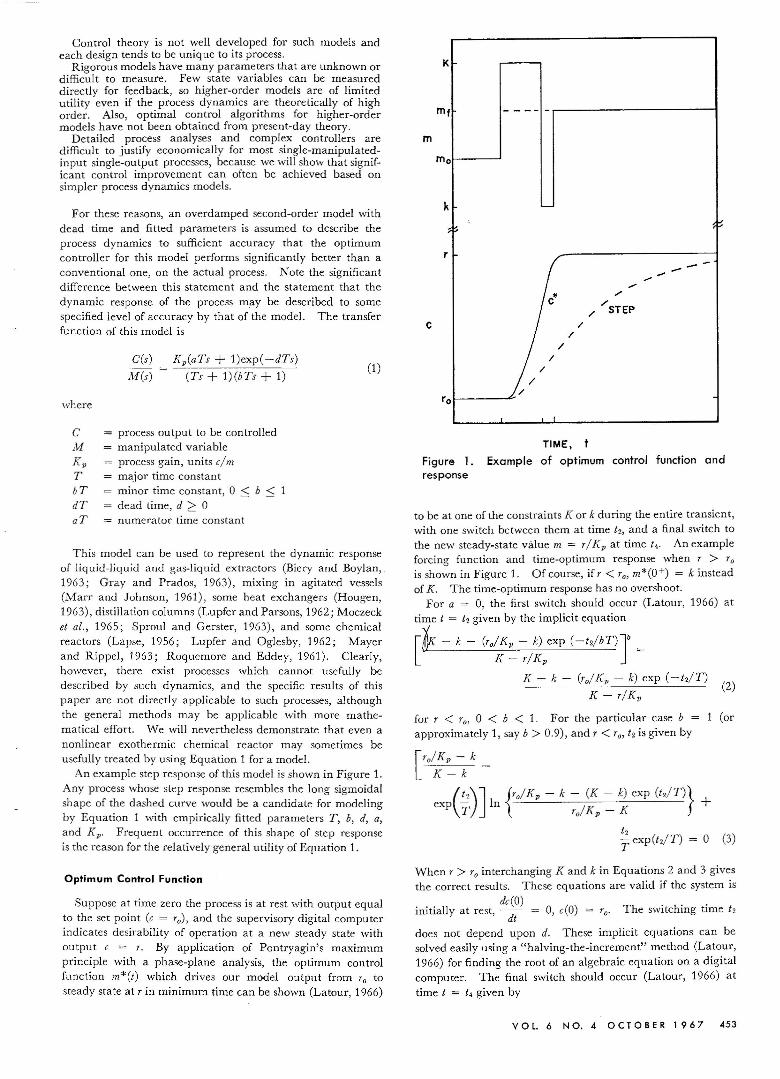
An example step response of this model is shown in Figure 1.Any process whose step response resembles the long sigmoidalshape of the dashed curve would be a candidate for modelingby Equation 1 with empirically fitted parameters T, b, d, a,and Kp. Frequent occurrence of this shape of step responseis the reason for the relatively general utility of Equation 1.

Optimum Control Function

Suppose at time zero the process is at rest with output equalto the set point (c = To), and the supervisory digital computerindicates desirability of operation at a new steady state withoutput c = T. By application of Pontryagin's maximumprinciple with a phase-plane analysis, the optimum controlfunction m*(t) which drives our model output from To tosteady state at r in minimum time can be shown (Latour, 1966)

m f - - -- -

0

-c ~~~

-- -". ----

"c·,-

;' /STEP/

//

I/

//

0

K

m

m

k

r

c

(1)

r

Figure 1.response

TIME,

Example of optimum control function and

to be at one of the constraints K or k during the entire transient,with one switch between them at time 12, and a final switch tothe new steady-state value m = T / Kp at time t«. An exampleforcing function and time-optimum response when T > Tois shown in Figure 1. Of course, if T < To,m*(O+) = k insteadof K. The time-optimum response has no overshoot.

For a = 0, the first switch should occur (Latour, 1966) attime t = t2 given by the implicit equation

[&K - k - (ro/Kp - k) exp (-tdbT)Jb =

K - r/KpK - k - (ro/ K; - k) exp (-t2/T)

(2)K - T/Kp

for r < 1'0' ° < b < 1. For the particular case b = (orapproximately 1, say b > 0.9), and T < To, t2 is given by

[To/Kp - k _

K - k

(t2)J {To/Kp - k - (K - k) exp (t2/T)}

exp T In TjKp - K +

When T > Tointerchanging K and k in Equations 2 and 3 givesthe correct results. These equations are valid if the system is

dc(O)initially at rest, -- = 0, c(O) = To' The switching time 12

dtdoes not depend upon d. These implicit equations can besolved easily using a "halving-the-increment" method (Latour,1966) for finding the root of an algebraic equation on a digitalcomputer. The final switch should occur (Latour, 1966) attime t = t4 given by

VOl. 6 NO. 4 0 C TO BER 1 9 67 453

t41T =

[ro/ Kp - k - (K - k) eXP(t2IT)]

In rlKp-K ,r<ro

['olKp - K - (k - K) exp(t'/T)]

In rlKp-k ,r>ro

where ° < b ::;; 1. t, is also independent of d. Equations2, 3, and 4 are obtained from solutions of the differentialequations defined by Equation 1 for m = K and m = k,Derivations are given by Koppel and Latour (1965).

For a first-order system (b = 0) with dead time, no switchingreversal is required, and the single switch to the final steady-state m = rIK p should occur at t = t2 = t ; given by

[rolKp - kJ r < ro (5)In I 't21T =

r Kp - k

[rolKp - KJ (6)In rlKp - K ' r > '0

Our experience suggests that Equations 5 and 6 can be used forsecond-order systems when b < 0.1.

The effect of the minor time constant on switching times isshown in Figure 2 for two set-point change magnitudes.Values of K = 1, k = 0, T = Kp = 1 were assumed to preparethe graph.

The minimum response-i.e., the minimum time to drivethe output from r, to steady state at r-is

t5 = t; + dT (7)

since an additional delay time after the return at I; to m =rlKp is required to complete the transient. After time t5

has elapsed control should be returned to conventional closed-loop regulator control. The PID controller should notintegrate the error during bang-bang control. This may beachieved easily on the newer conventional controllers equippedwith "bumpless transfer" from manual to automatic modes.During the bang-bang forcing, the computer should switch thecontroller to the manual mode. At i, the computer shouldset met) at rl Kp, set the controller set point at the new desiredvalue, and switch the controller to the automatic mode attime ts. If in addition to the supervisory action, direct digitalcontrol is used in place of the conventional instrument, asimilar implementation is easily achieved.

Knowing the constants ro, r, K, and k, and the model pa-rameters, we can determine the optimum control m*(t) bycalculating t2 and t4 from Equations 2 and 4. If an on-linedigital computer is not available .. the bang-bang control can beimplemented manually from a table or graph of t2 and t;, asfunctions of ro and r prepared off-line. Analog timing circuits(Latour, 1964) which solve these equations can be used togenerate m*(t) directly.

FiHing Model Parameters

Experimental modeling techniques to obtain Gp(s) have beengenerally based on step, pulse, or frequency response data(Hougen, 1964). However, for expedience and to simplifycomputations, we propose that the process be forced in abang-bang fashion as in Figure 1 with guessed values of t2and I;. These values of 12 and t4 will not give an optimumresponse but they can be easily estimated from Equations2 and 4 using rough estimates of T, b, and Kp perhaps obtainedfrom a step response (Harriott, 1964; Latour, 1966), or chosenduring the transient by a skilled process operator using his"feel" for the process response to guide his switching times.

454 I & E CPR 0 C ES S DES I G NAN DOE VEL 0 P MEN T

(4)r • 0.65

roO 0.51.2

0.8

t~ __ -,/

/" -,/ --,..."...---/--- »>

#' .--/f.-/ /'r

/O~----L- ~ ~ -L ~o 0.2 0.4 0.6 0.8 1.0

MINOR TIME CONSTANT, b

Figure 2. Effect of minor time constant onswitching times

K = T = Kp = 1, k = 0

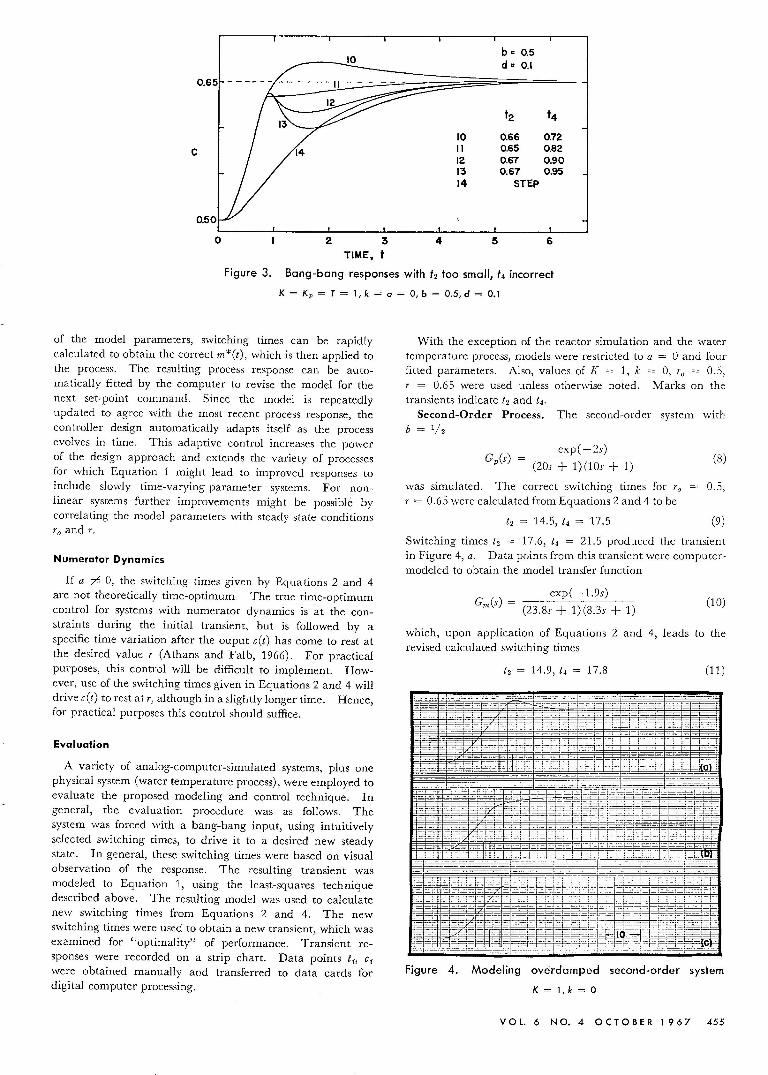
Some bang-bang responses shown in Figure 3 obtained from anormalized system (K = Kp = T = 1, k = a = 0, b = 0.5,d = 0.1) when t2 is too small and t; is in error, can be com-pared with the optimum response in Figure 1 (t2 = 0.74, t4 =0.89, 15 = 0.99). Switching times considerably in error (15%)still give responses which are not poorer than the simple stepresponse. It is not likely that the switching times intuitivelychosen by a skilled operator would cause a serious deteriorationin the test response compared to that of a conventional con-troller.

The model parameters can now be fitted in the time domainto the response data from bang-bang forcing with these in-correct (but known) switching times by nonlinear statisticalregression. The model response to the known forcing canbe written analytically in terms of the unknown parametersT, b, a, d, and Kp. To start the regression analysis, one canobtain reasonable estimates of the parameters from a stepresponse by means of graphical techniques such as the familiarone of Oldenbourg and Sartorius (1948). These estimateswere so close that convergence problems were never en-countered in this work. In our work, a digital computerprogram (Latour, 1966) based upon Marquardt's (1959)nonlinear regression was used to obtain the fitted modelparameters from data curves similar to Figure 3. The pa-rameters are chosen to minimize the sum of squares of devia-tion of the physical process response from Equation 1. Revisedswitching times can then be calculated from the model usingEquations 2 and 4.

This procedure is directly related to the control objective ofimproved set-point responses, since the model and processare made to agree on the type of input forcing which will beused for set-point control. Also, modeling can be a repetitiveprocedure if an on-line digital computer is available. Newset-point commands r are determined by the supervisorycomputer (a steady-state optimizer). With current estimates

b » 0.5d = 0.1

t2 t4

10 0.66 0.72

C II 0.65 0.8212 0.67 0.9013 0.67 0.9514 STEP

o 234 5 6TIME, t

Figure 3. Bang-bang responses with t2 too small, t4 incorrect

K = Kp = T = 1, k = a = 0, b = 0.5, d = 0.1

of the model parameters, switching times can be rapidlycalculated to obtain the correct m*(t), which is then applied tothe process. The resulting process response can be auto-matically fitted by the computer to revise the model for thenext set-point command. Since the model is repeatedlyupdated to agree with the most recent process response, thecontroller design automatically adapts itself as the processevolves in time. This adaptive control increases the powerof the design approach and extends the variety of processesfor which Equation 1 might lead to improved responses toinclude slowly time-varying-parameter systems. For non-linear systems further improvements might be possible bycorrelating the model parameters with steady-state conditionsTo and T.

Numerator Dynamics

If a r" 0, the switching times given by Equations 2 and 4are not theoretically time-optimum. The true time-optimumcontrol for systems with numerator dynamics is at the con-straints during the initial transient, but is followed by aspecific time variation after the ouput e(t) has come to rest atthe desired value T (Athans and Falb, 1966). For practicalpurposes, this control will be difficult to implement. How-ever, use of the switching times given in Equations 2 and 4 willdrive e(t) to rest at T, although in a slightly longer time. Hence,for practical purposes this control should suffice.

Evaluation

A variety of analog-computer-simulated systems, plus onephysical system (water temperature process), were employed toevaluate the proposed modeling and control technique. Ingeneral, the evaluation procedure was as follows. Thesystem was forced with a bang-bang input, using intuitivelyselected switching times, to drive it to a desired new steadystate. In general, these switching times were based on visualobservation of the response. The resulting transient wasmodeled to Equation 1, using the least-squares techniquedescribed above. The resulting model was used to calculatenew switching times from Equations 2 and 4. The newswitching times were used to obtain a new transient, which wasexamined for "optimaIity" of performance. Transient re-sponses were recorded on a strip chart. Data points ti, Ci

were obtained manually and transferred to data cards fordigital computer processing.

With the exception of the reactor simulation and the watertemperature process, models were restricted to a = 0 and fourfitted parameters. Also, values of K = 1, k = 0, To = 0.5,T = 0.65 were used unless otherwise noted. Marks on thetransients indicate t2 and ts,

Second-Order Process. The second-order system withb = 1/2

exp( -25)Gp(S) = (205 + 1)(105 + 1) (8)

was simulated. The correct switching times for To 0.5,T = 0.65 were calculated from Equations 2 and 4 to be

t2 = 14.5, t4 = 17.5 (9)

Switching times t2 = -17.6, t4 = 21.5 produced the transientin Figure 4, a. Data points from this transient were computer-modeled to obtain the model transfer function

exp( -1.95)Gm(s) =

(23.85 + 1)(8.35 + 1)(10)

which, upon application of Equations 2 and 4, leads to therevised calculated switching times

t2 = 14.9, t4 = 17.8 (11)

, 1 -,- ,•-.

0- • _.

- .. - .• to.:- -I-:., ,.'"

, !--:.-sE 1"

- •. J

~-

1f".L =f=i= :!-=t

b~' -I??',=,=:_"33·-

Figure 4. Modeling overdornpe d second-order system

K=I,k=O

VOl. 6 NO. 4 0 C TO B ER 1 967 455

If the switching times are too short, the transient Figure 4, b,can result (t2 = 13.0, t4 = 14.9). This transient was fitted bythe model transfer function

exp( -2.2s)(12)Gm(S) = (21.6s + 1)(9.7s + 1)

which leads to the revised switching times from Equations 2and 4

t2 = 14.9, t. = 18.0 (13)

In both cases, these revised switching times would produce anexcellent response similar to Figure 4, c (tz = 14.7, t. = 17.8).Curves 4a and 4b resulting from positive and negative switchingtime errors were modeled by transfer functions somewhatdifferent from the analytical simulation (b = 0.35 and 0.45,respectively). However, the revised switching times agreewith each other and the analytical values, and result in theimproved transient in Figure 4, c. Switching times couldnot be reproduced manually with a stop watch as accuratelyas they could be measured from the chart recording of met)afterward; hence, the slight differences between predictedvalues and those actually used in Figure 4, c. The procedureis therefore seen to converge to essentially the optimum re-sponse after one modeling step in both cases. An earlierpaper (Latour, 1964) showed that the response of Figure 4, cand similar time optimum responses are faster than con-ventional set-point responses by an amount on the order ofT, the major process time constant.

An underdamped second-order system with ( = 0.707 wassimulated. Its response was modeled with b = 0.95 (orI = 1.0003). The predicted switching times when theprocess necessarily differed from the model still produced abang-bang response much improved over the step response.Modeling behavior for this process is of interest becauseHougen (1964) states that mixing a nonvolatile dye on platesof a commercial distillation column shows second-orderdynamics with 0.8 damping coefficient plus dead time. Hou-gen also states that mixing in long tubes and a variety of heatexchangers show second-order, critically damped tendencies«( = 1). Details are given by Latour (1966).

Third-Order Process. The response of the system

exp( -2s)Gp(s) = (20s + 1)(10s +-1-) (-6-s-+-1-) (14)

to arbitrarily selected switching times was modeled by

exp(-6.1s)(15)Gm(s) = (19.2s + 1)(13.4s + 1)

and yielded switching times which produced a very satis-factory response that was significantly improved over the set-point response of a conventional PID controller. Model deadtime is larger than process dead time to account for the thirdtime constant. Although switching times do not depend upond, including this parameter really allows the model to achievemore realistic time constants and a better fit. ,

Similarly satisfactory results were obtained (Latour, 1966)for the third-order system

(16)(r + 1)3

Tenth-Order System. Staged processing systems (traycolumns, extractors, etc.) exhibit high-order dynamics. Totest the modeling procedure and selection of switching timeson such a system, the tenth-order system

456 I&EC PROCESS DESIGN AND DEVELOPMENT

1Gp(s) = (10s + 1)10 (17)

was considered. The step response of this system was modeledgraphically to obtain

exp( -55s)Gm(s) = (40s + 1)(7s + 1)' t2 = 20.1, t4 = 22.9 (18)

The transient resulting from these switching times was fitteddigitally to obtain the model

Gm(s) = exp(-51s)(27s + 1)(24s + 1)

t2 = 25.4, t4 = 31.2, d = 1.89, b = 0.9

(19)

The transient using these switching times was considerablyimproved over the step response and the response based on thefirst set of switching times in Equation 18. This improvementmay be described in terms of the 10% settling times as definedby Coughanowr and Koppel (1965). The settling times forthe step response and the response based on the switching timesof Equation 18 are 142 and 153, respectively; the settling timefor the response based on the switching times of Equation 19 is90. Further details on these responses are given by Latour(1966).

Nonlinear Exothermic Reactor. Further study of theutility and limitations of the design procedure was attempted bymodeling a highly nonlinear, exothermic reactor simulation.Orent (1965) simulated and controlled a modified version of theAris-Amundson (1958), Crethlein-Lapidus (1963) continuousstirred-tank reactor, for the irreversible exotheric reaction

kA -+ B with first-order kinetics. The modification involvedaddition of cooling coil dynamics. The reaction rate constantis

k koexp ( - E/ Re) (20)

where

k Arrhenius reaction rate constant, sec."?ko frequency factor, 7.86 X 1012, sec.-1

E activation energy, 28,000 cal./moleR gas constant, 1.987 cal./mole - a K.e absolute temperature of reactor, a K.

The mass balance on the reactor contents assuming uniformmixing is

dEV - = FE - FE - VkEdt 0

(21)

where

V material volume, 1000 cc.E concentration of A in exit, moles/cc.Eo concentration of A in inlet, 6.5 X 10-3 mole/cc.F volumetric flow, 10 cc./sec.

If we assume no heat transfer with the surroundings, and thephysical properties of inlet and outlet streams identical, theenergy balance is

deVPCT - = FpCT(eo - e)

dt_ !:::.HVkE _ UA(ec ~_!!co)

In(~)e - ec

(22)

where

p density, 1 g./cc.

e= heat capacity, 1 cal./g. - 0 K.

temperature of reactor and exit stream, 0 K.temperature of inlet stream, 3500 K.exothermic heat of reaction, 27,000 cal./moleover-all heat transfer coefficient times cooling coil

area, 7 cal./sec. - 0 K.inlet coolant temperature, 3000 K.exit coolant temperature, 0 K.

e,-!1H =

UA

An approximate lumped energy balance for the cooling coil is

(23)

with

Ve coil volume, 100 cc.Pe coolant density, 1 g./cc.rre coolant heat capacity, 1 cal./g. 0 K.Fe coolant flow, 0 ~ Fe ~ 20, cc./sec.

This cooling coil equation is added to impart higher orderdynamic effects. The manipulated variable is the boundedcoolant flow rate. The output temperature was delayed by asecond-order Pade circuit to introduce an additional 6-seconddead time, representative of higher-order lags. Only controlabout the stable high temperature steady-state

4600 K.4190 K.0.162 X 10-3 mole/cc.5.13 cc./sec.

is considered here.second steps in Fe.

Orent reports responses to ± 1 cc. perHe modeled these by

6.1exp(-11s) OK.

70s + 1 cc.y'sec,(24)

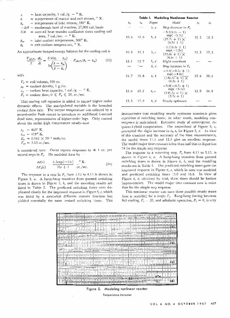
The response to a step in Fe from 5.13 to 4.13 is shown inFigure 5, a. A bang-bang transient from guessed switchingtimes is shown in Figure 5, b, and the modeling results arelisted in Table 1. The predicted switching times were du-plicated closely for the improved response in Figure 5, c, whichwas fitted by a somewhat different transfer function butyielded essentially the same revised switching times. This

Table I. Modeling Nonlinear Reactort, t , Figure Model I, 14

5, a Step decrease in F,

-5.1(0.ls + 1)10.6 12.6 5, b

exp( -5.7s) 11.1 12.3(25.7s + 1) X

(6.9s+ 1)

-5.7(0.3s + 1)10.9 12.1 5, c

exp( -7.0s) 11.3 12.3(33.0s + 1) X

(4.6s + 1)12.1 12.7 5, d Slight overshoot

6, a Step increase in Fc-4.4(-0.5s + 1)

14.7 15.8 6, bexp( -4.0s)

12.6 20.1(126.4s + 1) X(6.2s + 1)

-5.0( -0.7s + 1)

12.6 20.2 6, cexp( -5.1s)

12.0 16.8(141.2s + 1) X(3.7s + 1)

12.5 17.9 6, d Nearly optimum

demonstrates that modeling nearly optimum transients givesrepetition of switching times; in other words, modeling con-vergence is maintained. Extensive study of convergence re-quires hybrid computation. The undershoot of Figure 5, c,prompted the slight increase in t-i, t.l for Figure 5, d. In viewof this transient and the accuracy of the time measurements,the model times 11.3 and 12.3 give an excellent response.The model major time constant is less than half that in Equation24 for the simple step response.

The response to a returning step, Fe from 4.13 to 5.13, isshown in Figure 6, a. A bang-bang transient from guessedswitching times is shown in Figure 6, b, and the modelingresults are in Table 1. The predicted switching times gave theimproved response in Figure 6, c, which in turn was modeledand predicted switching times 12.0 and 16.8. In view ofFigure 6, d, obtained by trial, these times should be furtherimprovements. The model major time constant now is twicethat for the simple step response.

This nonlinear reactor can have three possible steady states(one is unstable) for a single Fe. Bang-bang forcing betweenfull cooling, Fe = 20, and adiabatic operation, Fe = 0, is very

~~.~~i-

j--"ji-~:t:::::- ~~ .. ;~3,.lc

:C-L_

; ~.--I

Figure 5. Modeling nonlinear reactor

Temperature increases

VOL. 6 N O. 4 0 C T 0 B ER 1 9 67 457

Figure 6. Modeling nonlinear reactor

Temperature decreases

severe. Increasing temperature reponses requiring Fe = 20initially are faster than the returning responses requiring Fe =20 initially.

This work illustrates a limitation of the method if design isrestricted to fixed model parameters, and the system is highlynonlinear, since the parameters depend upon direction.Nevertheless, the bang-bang response of this reactor between4600 and 4660 K. can be fitted to a second-order dead timetransfer function which predicts improved switching times.Although modeling convergence is not quite complete in onestep as for the linear systems, the response is acceptable andmuch superior to the simple step response. The adaptiveprocedure described above would require a simple modificationto allow the computer to use two different models, one for

increases in Fe and the other for decreases. The rigoroustime-optimum control of similar nonlinear reactors was studiedby Siebenthal and Aris (1964).

In general, the nonlinear effects of temperature and chemicalkinetics make reactor models complex and optimum controldifficult. However, in some cases the nonlinearities are notpronounced, and a simple linear method such as that suggestedhere might be adequate for process control purposes. Thecracking furnace studied by Lapse (1956), the commercialpolymerization reactor for synthetic rubber studied by Roque-more and Eddey (1961), the large compartmentalized poly-merization reactors tested by Mayer and Rippel (1963), andthe catalytic polymerization in a solvent reported by Lupferand Oglesby (1962) are good examples for application. Even

?r EXPERIMENT IN AUTOMATIC PROCESS CONTROL.~~. fLOW DIAGRAMTO

DRAiN'-

~N'AOT_ FL~ ,,,[

~rc- ~

0 SUPPlY r r"T~

= ...:\~.:.- c::c:J~ POWER I--- COHTROLl..ER

V -IIO~TEll -

TC2

10==POWERMETER

SUPPLY Q~~1 ~ r----== II DEADTIME .~

l1IHK IWATERLJ~ ©r= ANALOG

MANIFOLD ~ COMPUTER

220 "-

POWER'~ r- •._Jl.OlD I£XfER METER

VARIAC •.• ~.I '. ....-- I8AYCHET RESlSWOCE I

LEGEND HEATER I~~B~@r =kj"-rou-i f-=><== GATE 'oIALVE

=-= G~OBE VALVE110 ""--- INS~'" LIlIES ~

== POWER LINES POTENTIOMETER RECORDER_TC3 THERMOCOUP!.E LOAD HEATER

TANKZ ~oo~ TRANSMITTER CONTROLl..ER. VARIAC POWER toIETER

Figure 7. Experiment in automatic processcontrol flow diagram

458 I & E CPR 0 C ES S 0 E S I G NAN DOE VEL 0 PM E N T

I ; : ; : :...:..;_~~~ : : ; : .

.:':: ~;:~-i

Figure 8. Experimental responses from water temperature process

Figure 9. Optimum bang-bang responses from water temperature process

for the highly nonlinear reactor discussed above, acceptableresults are obtained from the linear techniques.

Water Temperature Process. A temperature controlsystem for a water flow process with two agitated vessels and aconnecting pipeline (Figure 7) was used to test this controltechnique. A.-c. power to a 2-kw. heater in the first tank wasmanipulated to control the temperature of water leaving thesecond tank. Water volumes and flows were maintainedapproximately constant. A theoretical model obtained fromdifferential lumped energy balances and physical properties is

(J(s) 12.09 exp( -24.7s) 0 /

- F. kw.Q(s) (151.8s + 1) (81.0s + 1)

(25)

In terms of the parameters of the general model of Equation 1,we have d = 0.162, b = 0.533, a = O. Time constants are inseconds. More details of the process are given by Latour(1966).

A response with 29% overshoot to bang-bang forcing (notshown) with 12= 125 seconds, 14= 155 seconds was fitted bythe model

G () _ 12.6( -0.2s + l)exp( -25.5s) 0 /m s - F. kw.

(159.1s + 1)(95.5s + 1)(26)

in excellent agreement with Equation 25. This model yieldsrevised switching times 12 = 99, 14 = 139 for the same tem-perature change (-3.160 F.). These switching times wouldundoubtedly reduce the overshoot. An improved responsewith 13% overshoot using 12= 111,14 = 134 is shown in Figure8, a. This was fitted by the model

13.5(1.4s + 1) exp( -25.9s) 0

Gm(s) = ( F.j kw. (27)164.6s + 1) (9S.4s + 1)

which yielded revised switching times 12 = 109, I, = 149.Because steady-state conditions are difficult to repeat exactly,the procedure followed in the simulation tests, wherein therevised switching times were used in an otherwise identicaltest, could not be used in these experimental tests. However,the revised switching times are clearly in the right direction,and would tend to reduce the slight overshoot in Figure 8, a,which is already a distinct improvement over the simple stepresponse of Figure 8, b. The final steady-state values areindicated at the left of each transient.

The excellent responses in Figure 9 were obtained from theprocess using switching based upon the theoretical modelEquation 25 and returning to closed-loop proportional-integral-derivative control after the final value was reached.

Conclusions

Improved set-point responses can be achieved, for processeswhose dynamics can be represented as overdamped second-order with dead time, by driving the manipulated variablein a bang-bang fashion using two switching times. Algebraicequations for these switching times (one is implicit) are givenin terms of the model parameters (two time constants andgain), the manipulated variable saturation constraints, andthe starting and desired values of the output. The modelparameters can be obtained from bang-bang type responsedata (using non optimum switching times) by nonlinear re-gression. The design procedure gave satisfactory results whenevaluated with a variety of processes, some differing widelyfrom the assumed model, plus one physical system. It isanticipated that the method will be particularly useful whenincorporated into a supervisory digital control system.

VOl. 6 NO. 4 0 CT0 8 ER '9 6 7 459

Acknowledgment

P. M. Aiken assembled the experimental equipment.

Literature Cited

Aris, R., Amundson, N. R., Chern. Eng. Sci. 7, 131 (1958).Athans, M., Falb, P. L., "Optimal Control," McGraw-Hili,

New York, 1966.Biery, S. C., Boylan, D. R., IND.ENG.CHEM.FUNDAMENTALS,2,

44 (1963).Coughanowr, D. R., Koppel, L. B., "Process Systems Analysis and

Control," McGraw-Hill, New York, 1965.Crowther, R. H., Pitrak, J. E., Ply, E. N., Chern. Eng. Progr. 57,

No.6, 39 (1961).Gibson, J. E., Johnson, C. D., IEEE Trans. Auto. Contr. AC-8,

No.1, 4 (1963).Gray, R.I., Prados, J. W., A.l.Ch.E.J. 9, No.2, 211 (1963).Grethlein, H. E., Lapidus, L., A.l.Ch.E.J. 9, No.2, 230 (1963).Harriott, P., "Process Control," McGraw-Hill, New York, 1964.Hougen, J. 0., Chern. Eng. Progr. Monograph SeT. 4,60 (1964).Hougen, J. 0., Chern. Eng. Progr. 59, 49 (1963).Koppel, L. B., Latour, P. R., IND. ENG. CHEM.FUNDAMENTALS,

4,463 (1965).Lapse, C. G., ISA J. 3, 134 (1956).Latour, P. R., M.S. thesis, Purdue University, West Lafayette,

Ind., June 1964.Latour, P. R., Ph.D. thesis, Purdue University, West Lafayette,

Ind., June 1966.

Lefkowitz, I., Chern. Eng. Progr. Symp . Ser, 46, 59, 178 (1963).Lupfer, D. E., Oglesby, M. W., ISA Trans. 1, No.1, 72 (1962).Lupfer, D. E., Parsons, J. R., Chern. Eng. Progr. 58 No.9 37

(1962). ', ' ,Marquardt, D. W., Chern. Eng. Progr. 55, 65 (1959).Man, G. R., Johnson, E. F., Chern. Eng. Progr, Symp, Ser. No. 36

57, 109 (1961). ' ,Mayer, F. X., Rippel, G. R., Chern. Eng. Progr. Syrnp. Ser . No. 46

59,84 (1963). ' ,Moczeck, J. S., Otto, R. E., Williams, T. J., Chern. Eng. Progr.

Symp . Ser., No. 55, 61, 136 (1965).Oldenbourg R. C., Sartorius, H., Trans. A.S.M.E., 70, 78 (1948).Orent, H. H., Ph.D. thesis, Purdue University, West Lafayette,

Ind., June 1965.Pontryagin, L. S., Boltyanskii, V. G., Gamkralidze, R. V., Misch-

chenko, E. F., "The Mathematical Theory of Optimal Proc-esses," Wiley, New York, 1962.

Roquemore, K. G., Eddey, E. E., Chern. Eng. Progr. 57, No.9,35(1961).

Siebcnthal, CD., Aris, R., Chern. Eng. Sci.19, No. 10,729 (1964).Sproul, J. S., Gerster, J. A., Chern. Eng . Progr . Symp; SeT., No. 46,

59,21 (1963).Williams, T. J., ISA J. 12, 9, 76 (1965).

RECEIVEDfor review October 31, 1966ACCEPTEDMarch 27, 1967

i\.I.Ch.E. Meeting, Atlantic City, N.J. Financial assistancereceived from Purdue University and the National Science Founda-tion.

NONINTERACTING PROCESS CONTROLSHEAN-LIN LIU

Central Research Division Laboratory, Research Department, Mobil Oil Corp., Princeton, N. J. 08540

A new technique for the design of noninteracting control systems c~n handle constraint conditions on the

control variabl~~~d can be applied to nonlinear problems. Two examples illustrate the design method.

The first concerns a nonisothermal chemical reactor. The second deals with the control of a plate-type

absorption column. It is demonstrated that one state variable can be moved from one point to another

without affecting the other state variables.

IN MULTlVARIABLEfeedback control systems, a change in onereference variable will usually affect all output variables.

In some applications (temperature control in a chemicalreactor, for example), one desires to design a noninteractingcontrol-that is, a system in which a variation of anyonereference input quantity will cause only the one correspondingcontrolled output variable (such as one state variable) tochange. The design of such systems was considered byBoksenbom and Hood (Tsien, 1954). Using matrix algebra,Kavanagh (1957), Freeman (1958), and Morozovskii (1962)discussed the transfer matrix of noninteracting control systems.Chatterjee (1960) considered noninteracting process controlusing an analog computer and standard three-mode processcontrollers. In all the above references only linear problemswere discussed, and constraints on control variables wereneglected. Petrov (1960) discussed a very special non-linear problem without constraints. .

Although noninteracting control is potentially a powerfultool for reducing the complexity of control systems, it hasseveral limitations, as discussed by Morgan (1958) and Mesa- Basic Theoryrovic (1964). The present procedure requires a complete Before discussing the design of noninteracting controldynamic model of the system and an on-line digital computer. systems, the classical approach to control of linear multi-

This paper a~nounces two new results: Certain nonlinear, variable processes (Freeman, 1958; Kavanagh, 1957) is re-unconstrained processes can (1) be made noninteracting over viewed. Since the process is linear, the control problem canthe entlre·statevanablespac·e in-a--~anner analogous to th:.::a:.:.t__ be discussed in terms of Laplace transformed variables. In a

-foriinear-sysTems, and(2)bec?n~!:.;.!!.edin-~p.iiCe~':-~~~-~9n- closed loop system, as shown in Figure 1, if P represents the

460 I & E CPR 0 C ES S DES I G NAN D D EVE ·L0 P MEN T

interacting way even when there are constraints on the process~.!lR-~_tyarI~l:iics::-----·-·---··--·-·-- ... - ..--------

Two examples illustrate the present method. The first dealswith a nonisothermal chemical reactor in which a second-orderirreversible chemical reaction, 2A -.. B, takes place. Theconcentration of component A and the temperature are to becontrolled by manipulating the flow rates of reactant andcoolant. Either state variable, temperature or concentration,can be moved from one point to another without affecting theother state variable.

In the second example, noninteracting control of a plate-typeabsorption column is considered. It is assumed that thereare seven plates in the absorption column and that one com-ponent in the gas phase is absorbed by liquid absorbent.It is demonstrated that, by manipulating the liquid flow rate,one can maintain the gas outlet concentration at a fixed valueeven if perturbations in the gas flow rate or the gas inlet con-centration occur.

I&EC

PROCESS DESIGN

AND DEVELOPMENT

VOL 6, NO.4, OCTOBER 1967

Editor: HUGH M. HULBURT

EDITORIAL HEADQUARTERSWashington, D. C. 200361155 16th St., N.W.Phone 202·737·3337

Manager, Manuscript Reviewing: Katherine I. Biggs

1Manager, Manuscript Editing: Ruth Reynard

Director of Design: Joseph Jacobs

Production Manager: Bacil Guiley

Layout: Herbert Kuttner

PRODUCTION-EASTON, PA.Associate Editor, Charlotte C. SayreEditorial Assistant, Jane M. Andrews

ADVISORY BOARD:Thomas Baron, Floyd L. Culler, Charles N. Satterfield

Associated Publications:

INDUSTRIAL AND ENGINEERING CHEMISTRY (monthly),David E. Gushee, Editor

I&EC FUNDAMENTALS (quarterly), Robert L. Pigford,Editor

I&EC PRODUCT RESEARCH AND DEVELOPMENT (quarterly)Rodney N. Hader, Acting Editor '

AMERICAN CHEMICAL SOCIETY PUBLICATIONS

Director oj Publications: Richard L. Kenyon

Director of Business Operations: Joseph H. Kuney

Publication Manager, Journals: David E. Gushee

Executive Assistant 10 the Director of Publications:Rodney N. Hader

Circulation Detulopment Manager: Herbert C. Spencer

Assistant to the Director oj Publications: William Q. Hull

SUBSCRIPTION SERVICE: All communications related tohandling of subscriptions, including notification of CHANGE OFADDRESS, should be: sent to Subscription Service Department,American Chemical Society, 1155 16th St., N.W., Washington,D. C. 20036. Changes of address notification sbould include bothold and new addresses, with ZIP code numbers, and be accompaniedby mailing label from a recent issue. Allow four weeks for changeto become effective.

SUBSCRIPTION Canada <&RATES PUAS FOrti&n

POJrag' iI~

SUBSCRIPTION RATES, I&EC PROCESS DESIGN ANDDEVELOPMENT, 1967:

Af,uric(lJ} Cb4mic(l1 Socitfy

M,mb"sNonm,mb"s

$5.00$10.00

SO.5O$050

$1.00$1.00

Single Copies: current, $3.00. Postage: Canada. $O.15i foreign,$0.20., Races for back issues or volumes are available from SpecialIssues Sales Depr., 1155 16th se, N.W., Washiogcoo, D. C. 20036.Claims for missing numbers will DOt be allowed if received morethan 60 days from date of mailing plus time normally required forpostal delivery of journal and claim. No claims allowed because offailure to notify the Subscription Service Department of ••.change ofaddress, or because copy is "missing from files."

Published quarterly by the American Chemical Society, from 20thand Northampton Srs., Easton, Pa. 18042. Second class postagepaid at Easton, Pa.

GUIDE FOR AUTHORS, publisbed 00 ioside back cover 01 eachissue, gives copy requirements for manuscripts. Submit three copiesto Manager, Manuscript Reviewing, L&EC, 1155 16th Sr., N.W.,Washington. D. C. 20036.

© Copyright 1967 by rbe American Chemical Society. Reproductionforbidden without permission.