To Sleep, Perchance to Dream: Prices for Funeral Homes in ... · To Sleep, Perchance to Dream:...

To Sleep, Perchance to Dream:

Prices for Funeral Homes in US States

by

Paolo Canofari

Dipartimento di Economia Diritto e Istituzioni, Università di Roma Tor Vergata

Giancarlo Marini

Dipartimento di Economia Diritto e Istituzioni, Università di Roma Tor Vergata

Pasquale Scaramozzino

Department of Financial and Management Studies, SOAS, University of London

and Dipartimento di Economia Diritto e Istituzioni, Università di Roma Tor Vergata

November 2012

Abstract

The need for a proper burial is widely felt. This paper makes use of an original data set to explore the relationship between the prices of cemetery plots and the prices of housing. It considers a simple model where the services from both real estate and funeral homes enter individuals’ utility function, and derives testable propositions in order to analyse the relation between housing when alive and after death. The services from funeral homes and from conventional housing are complements in the households’ utility. On the other hand, the services from funeral homes are an inferior good: a lower personal income is associated with higher grave prices.

Acknowledgements

We are grateful to Fabrizio Adriani, Barbara Annicchiarico, Leonardo Becchetti, Luisa Corrado, Ciaran Driver and Alessandro Piergallini for very useful comments. We remain responsible for any mistakes.

1

“All’ombra de’ cipressi e dentro l’urneconfortate di pianto è forse il sonno della morte men duro? […]Ma perché pria del tempo a sé il mortale invidierà l’illusïon che spentopur lo sofferma al limitar di Dite? Non vive ei forse anche sotterra, quando gli sarà muta l’armonia del giorno,se può destarla con soavi cure nella mente de’ suoi?”

“Shaded by cypresses, and kept in urns, Consoled by weeping, is the sleep of death Really not quite so rigid? [...] By why – before time does – must man begrudge Himself the illusion which, when he is dead, Yet stops him at the doorway into Dis? Buried, does he not go on living, with Day's harmony to him inaudible, If he rouse this illusion with sweet care In friendly memories?”

Ugo Foscolo, Sepulchres, translated by J. G. Nichols

1. Introduction

The need for a proper burial has ancient roots. Egyptian tombs, for example, have revealed

the extreme importance attached to life after death. Bodies had then to be preserved for the

other life through embalming and, in case of damage, could be replaced by a statue of the

deceased often present in the tomb, together with jewels, perfumes and several beautiful

accessories to accompany the deceased towards his new life. Notable examples of burial

practices in the first millennium B.C. are Etruscan Necropolises like Tarquinia, which

contains 6,000 graves cut in the rock. The beauty of the painted tombs is such that only short

visits are allowed in order to preserve such art treasuries for future generations. Burial was

necessary for the Greek to be admitted straight to the reign of Hades: otherwise the souls of

the dead would be damned to wander for eternity by the river Styx, the entrance to the

Underworld.

Roman catacombs, extending for about 40 kilometres, are still a place of incredible

suggestion for any visitor. In more recent times, in the western world, other than being a

prerequisite for saving one’s soul, a burial in cemeteries was practiced both for reasons of

Centre for Financial & Management Studies | SOAS | University of London

2

hygiene and also to limit the distressing influence of death on life: hence, the dead has to be

nicely dressed to look like a living body not to create excessive embarrassment (Ariés, 1975).

Burial practices and funeral homes, in spite of their historical importance, have been

largely neglected by academics in the mainstream literature. As argued by Exley (2004), such

scarce attention may reflect the need of self preservation of society, where the only subjects

of interest are youth, health and efficiency. Studies on the architectural and geographic

aspects of cemeteries as “total landscapes” have also been rare (Francaviglia, 1971). Even

less attention has been paid to the issue by economists, with the notable exceptions of

Harrington and Krynski (2002) and Harrington (2007), who document the lack of

competition in the market for funeral services, and Case and Menendez (2009), who examine

funeral expenses by South African households. Economics, in spite of its reputation as “the

dismal science”, does hardly deal with the issue of death and burial: the infinitively lived

representative agent model is taught in every university and even when death is allowed, the

paradigm can be restored by assuming that altruistic generations are linked by a perfect chain

of gifts and bequests. In the absence of bequests, people indeed die as in the finite horizon

continuous time overlapping generations model by Blanchard (1985), but the word death is

never mentioned. Buiter (1988) does explicitly illustrate the demographic properties of that

model and the word death appears even in the title; however, people remain perpetually

young till the passing out date.

The economics of funeral homes has been totally ignored in the literature, perhaps on

the grounds that homo economicus should not really bother. Yet this does not take into

account their overwhelming historical importance: most social and religious norms, at least in

Western countries, require that dead bodies should be properly buried after death. In

countries where prices of funeral homes are regulated there are typically controversies over

the assignment of rights to buy graves.

In an unregulated market like the US, it is not uncommon to find advertisements of

funeral home exchange due to moving to a different State. The importance of the funeral

housing market is proved by the fact that nearly 30% of the US population already own some

kind of cemetery property. Furthermore, at the current death rate of 0.8% there is an

estimated need for 1.76 million burial or entombment spaces per year. According to the Final

Arrangements Network, each year about 1.5 million people look for a cemetery property in

To Sleep, Perchance to Dream: Prices for Funeral Homes in US States

3

USA1. Grave Solutions estimates that there are over a million cemetery spaces available

nationwide.

Our key data set is based on the asking prices listed by Grave Solutions, a business

founded in 1996 which has developed a large resale programme for the sale of cemetery

property. Most funeral homes are not allowed to offer a discount from their general price list.

Hence, the prices at which cemetery plots are sold by funeral homes may not be consistent

with market clearing. However, the prices at which cemetery spaces are exchanged through a

resale programme would reflect more closely the balance between the demand for and the

supply of funeral plots.

We have collected the selling price offers for all US states provided by Grave

Solutions in December 2010. In total, we obtained data on 10,674 advertisements. These

include information on the cemetery name, the city, the state, the property type, and the price.

It is also reported whether the transaction refers to a direct sale, or whether Grave Solutions is

acting as a broker. The latter transactions have been excluded from the analysis, which

therefore only includes direct sales.

We have also collected data on house prices, in order to be able to compare their

prices with grave prices. A data set on real estate selling price have been constructed from

Trulia Real Estates, which reports prices on house prices by neighbourhood, city, county, and

state. The information on house prices has then been matched with the data on grave prices to

explore their comovement and their joint determinants.

We set forth a simple model where the services from both real estate and funeral

homes enter individuals’ utility function, and derive testable propositions in order to analyse

the relation between housing when alive and after death. In the empirical analysis we control

for a number potential determinants of the price of housing, such as demographic or religious

variables.

The structure of the paper is as follows. Section 2 outlines a simple utility model with

a demand for both conventional and funeral housing services. Section 3 describes the data

used in the analysis. Section 4 discusses the main empirical findings: the services from

funeral homes and from conventional housing are complements in the households’ utility, but

1 Private communication by Final Arrangements Network to the authors. The Network provides funeral and cremation services and lists plots for purchase and for sale across the USA.


4

the services from funeral homes are an inferior good in household’s utility. Section 5 carries

out a number of robustness tests for our results. Section 6 concludes.

2. Demand for funeral homes

We consider a very simple model where the individual lifetime utility function has as its

arguments the consumption of in-life, or conventional, housing services h1, the consumption

of after-life, or funeral housing services h2, and of a residual composite consumption

commodity, c:

(1)

The utility function is increasing in all its arguments and strictly quasi-concave.

The lifetime budget constraint takes the form:

(1)

where y is lifetime income, p1 and p2 are the prices of housing services and of funeral services

respectively, and where the price index for the residual consumption commodity has been

normalized to one.

The Marshallian demand functions for both housing services h1 and h2, which are

associated to the maximization of the utility function (1) subject to the budget constraint (2),

can be written as:

i = 1, 2 (3)

The corresponding price elasticities are defined as:

i, j = 1, 2 (3)

and the income elasticities as:

i = 1, 2 (4)


5

The relationships of complementarities and substitutability between housing services

can be expressed in terms of their cross-price elasticities , (Deaton and Muellbauer,

1980). In particular, in-life and after-life housing services are complementary if , and

substitutes if . A housing service is a necessity if the income elasticity of its

Marshallian demand function is less than one: , and a luxury if . Finally, a

housing service is an inferior good if the income elasticity of its Marshallian demand function

is negative: .

The key identifying assumption in the empirical analysis is that the price and quantity

variations across states of housing and funeral services are mainly related to changes in the

demand for these services. According to this interpretation, a positive relationship between

the prices of in-life and of after-life housing services is associated to a positive comovement

in the demand for these services, whereas a negative relationship is interpreted as being

associated to a negative comovement. The former case would correspond to conventional

housing and funeral services being complementary commodities in the households’ utility,

whist the latter case would correspond to these services being substitute commodities for

households.

3. The data

The original data set used in this paper has been constructed on the basis of 10,684

observations from Grave Solutions2. This is a network that provides information on cemetery

properties for sale offered by private parties, by cemeteries, and through brokerage services

in the US. In order to form a sufficiently large sample, we have collected all the

advertisements for sale that were published in December 2010. All the data have been

manually downloaded from the records reported in the website. The information which is

made publically available includes the cemetery name, the city and the state, the property

type, the price, the number of spaces or of crypts and whether Grave Solutions is acting as a

2 See the Data Appendix.


6

broker in the transaction. The property is classified as a mausoleum if it is above ground and

as a cemetery plot if it is below ground.

The main advantage of using Grave Solutions as our main source of data is that it has

developed a large resale programme for the sale of cemetery property. In the USA, most

funeral homes cannot offer a discount from their general price list. As a consequence, the

prices at which they sell their cemetery spaces may involve rationing on either side of the

markets, and may therefore not be fully consistent with market clearing. Since Grave

Solutions specializes on the resale of cemetery spaces, however, the prices at which these

spaces are exchanged are more likely to approximate the market clearing prices.

The variable on grave prices has been obtained by dividing the price of the cemetery

plot or of the mausoleum by the number of spaces. It is therefore a unit price per cemetery

space. The average unit grave price is US$ 2,261.941 and the median price is US$ 1,900.00,

with a standard deviation of US$ 2,021.226. All the observations for which Grave Solutions

is acting as a broker, and for which a transaction fee of 15% of the gross sale price is applied,

have been excluded from the sample. Our analysis therefore only includes those observations

which refer to a transaction between a buyer and a seller.

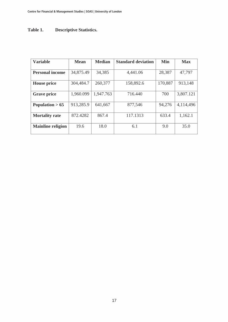
In the main econometric investigations in this paper, grave prices have been averaged

by state3. Table 1 summarizes key descriptive statistics for the main variables used in the

analysis. The average personal income in the sample of states is about $35,000. The average

house price is just over $300,000, whereas the average grave price is just short of $2,000.

Table 1 also gives details of population over 65, of the mortality rate, and of the percentage

of followers of mainline religion.

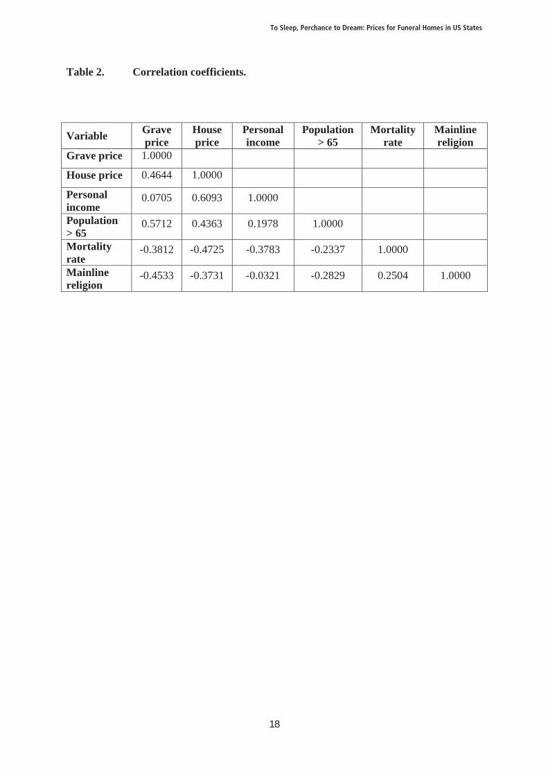
The correlation coefficients between pairs of variables are given in Table 2. The

average grave price is positively correlated with house price (the correlation coefficient is

0.4644) and with population over 65 years of age (the correlation is 0.5712). The correlation

with personal income is very weak (the correlation coefficient is only 0.0705). By contrast,

the average house price is strongly positively correlated with personal income (the correlation

is 0.6093). Both the average grave price and house price are negatively correlated with the

mortality rate and with mainline religion.

3 Please see the Data Appendix for a full description of all the variables used in the analysis and of their sources.


7

4. Empirical findings

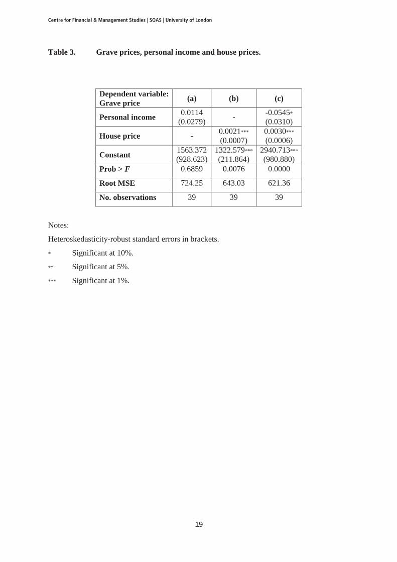
Table 3 presents the results of cross-section regressions over 39 US states of grave prices on

personal income and house prices. Column (a) shows that grave prices are positively related

to personal income: however, this relationship is not statistically significant. Column (b)

indicates that grave prices are positively related to house prices. When both regressors are

jointly included in column (c), grave prices are positively related to house prices but

negatively related to personal income, although the latter relationship is statistically not very

strong (p=0.087).

The results in Table 3 show that the prices for funeral homes tend to move in the same

direction as the prices for conventional housing, once personal income is controlled for. A

possible interpretation for this finding is that both types of housing services are regarded as

complements in the utility of households. A higher price of conventional housing services is

associated with an increased demand for housing: this also brings about an increase in the

demand for funeral housing, and therefore also higher levels of prices of grave spaces.

By contrast, the negative coefficient on personal income would suggest that higher

personal income is associated with lower, rather than higher, demand for funeral housing.

This could imply that the demand for funeral housing is an inferior good. When income is

low and households must switch their demand away from conventional housing services, they

turn to the more “affordable” services of funeral housing. Hence, a reduction in personal

income is associated with an increase in the demand for funeral services and higher grave

prices, and conversely an increase in income is associated with lower prices for funeral

homes.

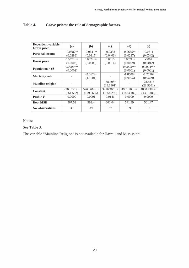
Table 4 explores the role of demographic variables on grave prices. Column (a)

considers population aged 65 or above as an additional explanatory variable. Its coefficient is

positive and highly significant, consistent with this age group being responsible for an

increased demand and thus higher prices. The total mortality rate in column (b) attracts a

negative coefficient, and is only significant at 10% (p = 0.069): lower mortality is thus

associated with higher expenditures on funeral services. Inclusion of mainline religion in

column (c) has a negative but not very significant coefficient (p = 0.056), and pushes both


8

personal income and house price into insignificance. Column (d) is our preferred

specification, with both population aged 65 and over and mortality rate included as

regressors. All variables are statistically significant and have the expected signs. In particular,

the coefficient on personal income is confirmed to be negative and the coefficient on house

price is positive. Column (e) also includes religion in the analysis, but this variable is not

statistically significant and reduces the precision of the estimates of the other coefficients in

the regression4.

5. Robustness of results

5.1. Bootstrapping

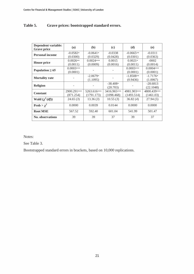
Because of the relatively small sample size in our data set, the sample test statistics may not

fully conform to the Gaussian distribution. We have therefore re-estimated all the standard

errors of the regression coefficients by bootstrapping the sample of observations. Table 5

reports the bootstrapped standard errors with 10,000 replications. All the results of Table 4

are confirmed. In particular, in column (d) the coefficients on personal income and on house

price are negative and positive respectively, and are both statistically significant. Population

over 65 and the mortality rate remain statistically significant and with the expected signs.

Religion is not significant once the demographic variables are included in column (e), and

again tends to reduce the precision of the other coefficients. Our results can therefore be

regarded as robust to departures from non-normality of the distribution of residuals which

could be related to the small sample of state observations at our disposal.

5.2. Robust regression

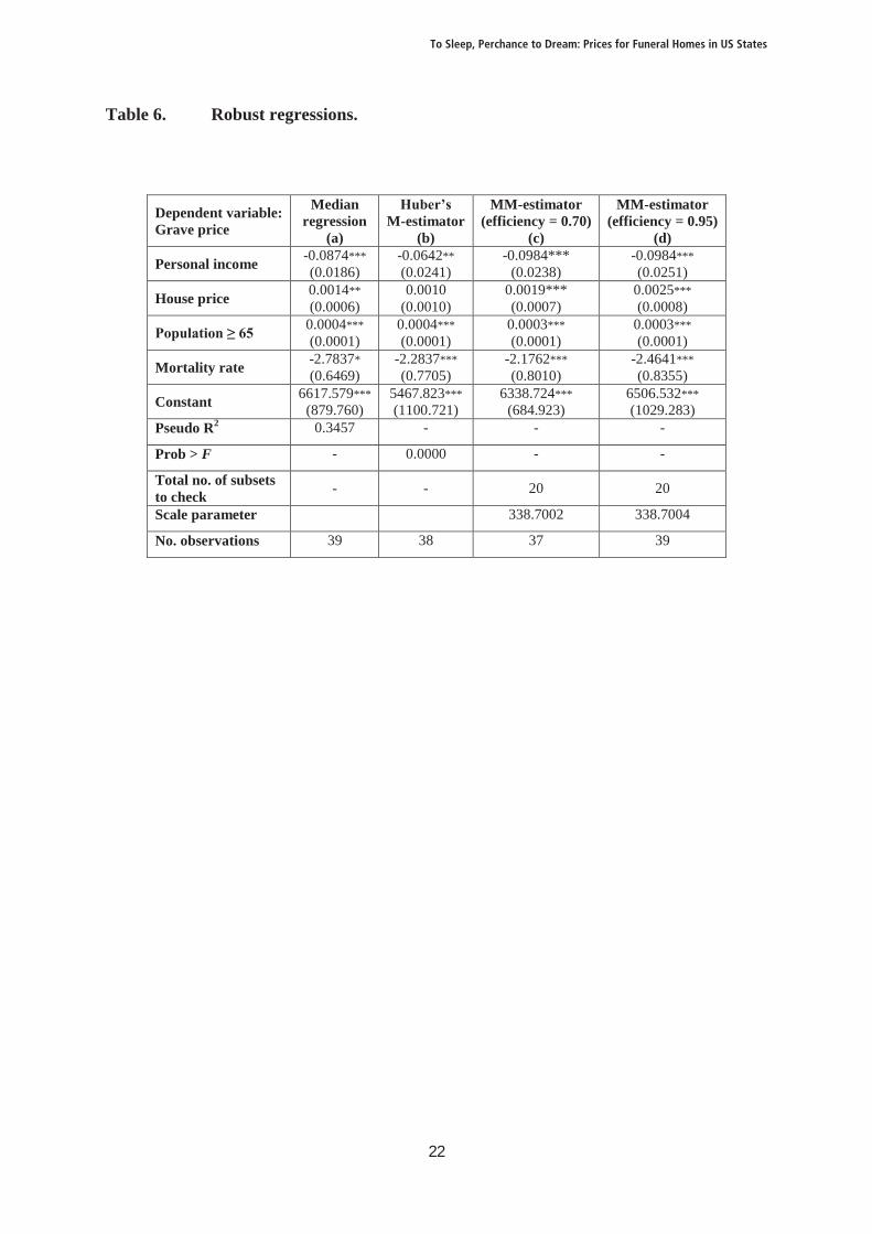
We have implemented a number of robust estimation methods in order further to validate our

key results. Column (a) of Table 6 presents the results of estimating re-estimating our

4 We introduced the cremation rate by state as an additional explanatory variable, but it was never statistically significant and did not affect the estimates of the other coefficients in the regressions. The results are available from the authors upon request.


9

preferred specification, column (d) from Table 4, using the median estimator (Koenker,

2005). This is regarded as a more robust estimator of location than LS, and is less sensitive to

potential outliers. Both the signs and the statistical significance of all the coefficients are

confirmed. Personal income and the mortality rate both attract a negative coefficient, whereas

the coefficients on personal income and on population aged 65 and above are both positive.

The results are therefore fully consistent with the discussion in Section 4.

Column (b) of Table 6 presents Huber’s (1964) monotonic M-estimator. This

minimizes a Tukey biweight loss function, in order to achieve increased efficiency whilst

maintaining robustness with respect to outliers. The coefficient on house price remains

positive but is now not significant, whereas all the other coefficients keep their signs and

remain statistically significant. The precision of the coefficient on the mortality rate is

actually improved by the M-estimator.

Columns (c) and (d) of Table 6 presents the results of the MM-estimation proposed by

Yohai (1987). These estimators are more robust to bad leverage points and are less likely to

converge to a local rather than a global minimum. They combine a high breakup point, i.e.

they are resistant to a potentially large number of outliers, with a high Gaussian efficiency5.

The guaranteed efficiency of the final estimates has been set to 70% and 95% in columns (c)

and (d) respectively. Both sets of estimates conform to the previous results. In particular, the

coefficient on personal income is negative, whilst the coefficient on house price is positive.

Both coefficients are highly significant.

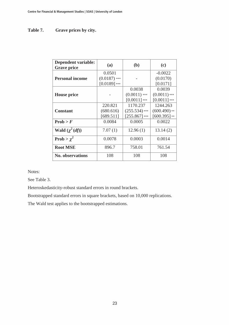
5.3. City regressions

In order to check the robustness of our results with respect to the level of aggregation, we

have re-estimated the relationships between grave prices, house prices and personal income

for a sample of 108 cities (see the Data Appendix for a full list of the cities included in the

analysis). The results are reported in Table 7. When simple regressions are estimated, both

personal income and house prices have a positive and significant effect on grave prices

(columns (a) and (b)). However, when both regressors are included the coefficient on

personal income becomes negative, albeit insignificantly so (column (c)). The standard errors

5 See also Verardi and Croux (2009) for a discussion of the properties of these estimators.


10

of the coefficients change very little when they are estimated by bootstrap methods (square

brackets in Table 7).

The findings on cities thus confirm the result that both types of housing services can

be regarded as complements in the utility of households. On the other hand, there is only

weak evidence for the notion that the demand for funeral housing is an inferior good, and that

higher personal income is associated with lower demand for funeral housing. The analysis of

the rôle of personal income on funeral homes will therefore require further investigation.

6. Conclusions

Burial makes death acceptable to society and keeps alive the memory of the dead ones. It is

commonly accepted that everyone should have a dignified burial and that dead bodies should

be buried without much delay. Once buried, corpses should not be disturbed although

disinterment can be allowed, in addition to legal needs, under motivated request of the

surviving spouse (who has the burial rights), such as when moving to a different state, in

order to be able to visit the funerary home. As stated by the Southampton City Council in the

UK, for example: “Many of us want to have a place we can visit our loved ones, and possibly

even be buried with them when the time comes”6.

The need to provide burial for close relatives is undisputable. In Sophocles’ tragedy

Antigone, the eponymous character accepts to face death by being buried alive in a cave, after

defying an order by the King of Thebes and offering the burial rites in honour of her dead

brother. It is even argued that the end of the civic community of Rome started inexorably

with the horror of unburied corpses after the battle of Philippi in 42 BCE, which saw Mark

Antony and Octavian defeat Marcus Junius Brutus and Gaius Cassius Longinus, who had

been responsible for the assassination of Julius Caesar7. The white bones left there without

any death ritual were in fact in sharp contrast with the notion that Roman citizens had the 6 http://www.southampton.gov.uk/living/southampton-ceremonies/funerals/burials/burialrights.aspx: accessed on 14 November, 2012. 7 “But all the daring sinners who, in defiance of the Gods’ will, profaned the pontiff’s head lie low in death, the death they merited. Witness Philippi and they whose scattered bones whiten the ground” (Ovid, 1931, Book 3, verses 705-708).


11

right to be buried, while the image of the mortal remains of Roman soldiers offering food to

wild animals and birds was an ignominious sign of moral decline, so much so that episode

was to become a political manifesto for emperor Nero (Barchiesi, 2002).

The societal need for funerary services also extends to relatives who died away or at

sea, as confirmed by the practice in France to write the name of the deceased sailor at sea on

a wax cross and to celebrate a funeral mass and service at home.

There is a human need to remain in touch with the deceased. Visiting funerary homes

and monumental cemeteries is a way to keep the memory and to transmit culture across

generations. For example, the American military Cemetery in Nettuno (Rome) attracts a very

large number of visitors each year, and so does the grave of Karl Marx in London.

The inscriptions on headstones are often evocative even for ordinary people, whose

alleged virtues are admittedly occasionally exaggerated. Many inscriptions indicate the will

to remain present in the memory of those left behind, such as that wanted on his grave by the

humorist writer Achille Campanile: “Torno subito” (“Back soon”).

Accommodation after death is thus a necessity for many societies, and the decision to

buy a funerary home should be a relevant issue in economics. About one third of Americans

already own a property when still alive, while most of the rest rely on their relatives to

provide it when the need arises. The market for cemetery property is an important one, with

two and a half million funeral homes per year needed to accommodate the deceased. Yet, its

economic implications have almost never been studied before.

The key result of our study is that the market for funeral homes is amenable to

standard economic analysis. Households make maximising decisions when it comes to decide

on their demand for funeral services, for themselves or for their dear ones. In particular, there

appears to be a link between the demand for funeral homes and the demand for housing. The

prices of graves and of houses are positively correlated, and their services are complements in

the households’ utility. On the other hand, there is evidence that funeral homes may be an

inferior good, with higher personal income being associated with lower prices of funeral

homes.

A large number of issues remains to be explored. For instance, it would be important

to endogenise the timing of the decision to purchase a funeral home. Why do 30% of

Americans buy their own cemetery property, and the remaining 70% do not? Do the latter


12

compensate for this by leaving larger bequests to their descendants? Answering these and

other questions is essential in order to understand the provisions that households make for the

event of their passing.

The questions posed above cannot be answered by the data set used in this paper, but

it is our belief that these are important issues which deserve to be addressed by economists.


13

References

Ariés, P. (1975), Essais sur l'Histoire de la Mort en Occident: Du Moyen Âge à Nos Jours,

Paris, Éditions du Seuil.

Barchiesi, A. (2002), “Mars Ultor in the Forum Augustum: A Verbal Monument, with a

Vengeance”, in G. Herbert-Brown (ed.), Ovid’s Fasti. Historical Readings at its

Bimillennium, Oxford, Oxford University Press, pp. 1-22.

Blanchard, O. (1985), “Debt, Deficits, and Finite Horizons”, Journal of Political Economy,

Vol. 93, No. 2, pp. 223-247.

Buiter, H. (1988), “Death, Birth, Productivity Growth and Debt Neutrality”, The Economic

Journal, Vol. 98, No. 391, pp. 279-293.

Case, A., and A. Menendez (2009), “Requiescat in Pace? The Consequences of High Priced

Funerals in South Africa”, NBER Working Paper No. 14998, May.

Deaton, A., and J. Muellbauer (1980), Economics and Consumer Behavior, Cambridge,

Cambridge University Press.

Exley, C. (2004), “Review Article: The Sociology of Dying, Death and Bereavement”,

Sociology of Health and Illness, Vol. 26, No. 1, pp. 110-122.

Francaviglia, R. V. (1971), “The Cemetery as an Evolving Cultural Landscape”, Annals of

the Association of American Geographers, Vol. 61, No. 3, September, pp. 501-509.

Foscolo, U. (1807), Dei sepolcri, Brescia, Bettoni; transl. by J. G. Nichols, Sepulchres,

Richmond, Oneworld Classics, 1995.

Harrington, D. E. (2007), “Preserving Funeral Markets with Ready-to-Embalm Laws”,

Journal of Economic Perspectives, Vol. 21, No. 4, Fall, pp. 201-216.

Harrington, D. E., and K. J. Krynski (2002), “The Effect of State Funeral Regulations on

Cremation Rates: Testing for Demand Inducement in Funeral Markets”, Journal of Law

and Economics, Vol. 45, No. 1, April, pp. 199-225.

Huber, P. (1964), “Robust Estimation of a Location Parameter”, Annals of Mathematical

Statistics, Vol. 35, No. 1, pp. 73-101.

Koenker, R. (2005), Quantile Regression, Cambridge (UK), Cambridge University Press.

Ovid (Publius Ovidius Naso) (1931), Fasti, transl. by J. G. Frazer, Loeb Classical Library,

Cambridge (MA), Harvard University Press, and London, William Heinemann Ltd.

Sophocles (1994), Antigone, transl. by Hugh Lloyd-Jones, Loeb Classical Library,

Cambridge (MA), Harvard University Press, and London, William Heinemann Ltd.


14

Verardi, V., and C. Croux (2009), “Robust Regression in Stata”, The Stata Journal,

StataCorp LP, vol. 9(3), September, pp. 439-453.

Yohai, V. J. (1987), “High Breakdown-Point and High Efficiency Robust Estimates for

Regressions”, The Annals of Statistics, Vol. 15, No. 20, pp. 642-656.


15

Data Appendix.

Variables and data sources.

Grave price: Unit price of cemetery plot (below ground) or of mausoleum (above ground), obtained by dividing the price of the plot or of the mausoleum by the number of spaces. Source: Grave Solutions. (http://www.gravesolutions.com/Default.asp)

House price: Price of homes for sale. Source: Trulia Real Estate.(http://www.trulia.com/home_prices/)

Personal income: Total disposable income in current US$ divided by mid-year population. Source: U.S. Department of Commerce, Bureau of Economic Analysis.(http://www.bea.gov/)

Population > 65: Total population aged 65 years and over. Source: U.S. Department of Commerce, United States Census Bureau. (http://www.census.gov/popest/)

Mortality rate: Number of death cases reported by 100,000 population. Source: National Center for Health Statistics. (http://wonder.cdc.gov/cmf-icd10.html)

Mainline religion: Percentages of each state’s population that affiliates with Mainline Protestant tradition. Source: The Pew Forum on Religion and Public Life, U.S. Religious Landscape Survey. (http://religions.pewforum.org/maps#)

List of states included in the analysis (39).

Alabama, Arizona, Arkansas, California, Colorado, Connecticut, Delaware, Florida, Georgia, Hawaii, Idaho, Illinois, Indiana, Iowa, Kansas, Kentucky, Louisiana, Maine, Maryland, Massachusetts, Michigan, Minnesota, Mississippi, Missouri, Nebraska, Nevada, New York, North Carolina, North Dakota, Ohio, Oklahoma, Oregon, Pennsylvania, South Carolina, Tennessee, Texas, Virginia, Washington, West Virginia.

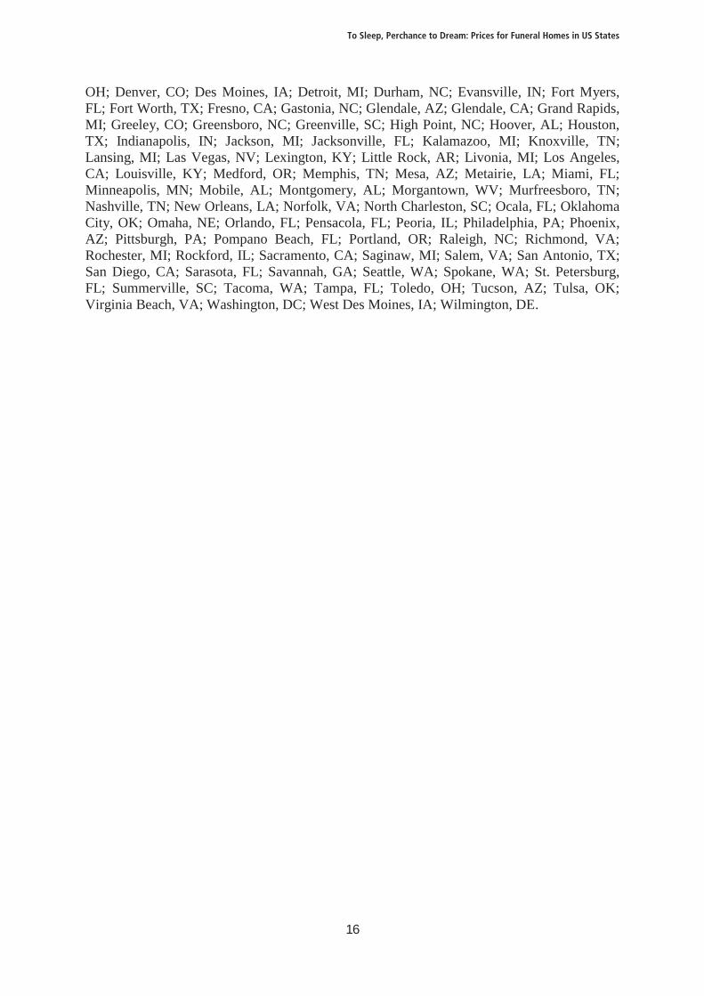
List of cities (108).

Adelphi, MD; Akron, OH; Alexandria, VA; Allentown, PA; Arlington, TX; Atlanta, GA; Augusta, GA; Aurora, CO; Austin, TX; Baltimore, MD; Battle Creek, MI; Bellevue, WA; Bethlehem, PA; Birmingham, AL; Bradenton, FL; Canton, OH; Charleston, SC; Charleston, WV; Charlotte, NC; Chattanooga, TN; Chicago, IL; Cincinnati, OH; Clearwater, FL; Cleveland, OH; Colorado Springs, CO; Columbia, SC; Columbus, OH; Dallas, TX; Dayton,


16

OH; Denver, CO; Des Moines, IA; Detroit, MI; Durham, NC; Evansville, IN; Fort Myers, FL; Fort Worth, TX; Fresno, CA; Gastonia, NC; Glendale, AZ; Glendale, CA; Grand Rapids, MI; Greeley, CO; Greensboro, NC; Greenville, SC; High Point, NC; Hoover, AL; Houston, TX; Indianapolis, IN; Jackson, MI; Jacksonville, FL; Kalamazoo, MI; Knoxville, TN; Lansing, MI; Las Vegas, NV; Lexington, KY; Little Rock, AR; Livonia, MI; Los Angeles, CA; Louisville, KY; Medford, OR; Memphis, TN; Mesa, AZ; Metairie, LA; Miami, FL;Minneapolis, MN; Mobile, AL; Montgomery, AL; Morgantown, WV; Murfreesboro, TN; Nashville, TN; New Orleans, LA; Norfolk, VA; North Charleston, SC; Ocala, FL; Oklahoma City, OK; Omaha, NE; Orlando, FL; Pensacola, FL; Peoria, IL; Philadelphia, PA; Phoenix, AZ; Pittsburgh, PA; Pompano Beach, FL; Portland, OR; Raleigh, NC; Richmond, VA; Rochester, MI; Rockford, IL; Sacramento, CA; Saginaw, MI; Salem, VA; San Antonio, TX; San Diego, CA; Sarasota, FL; Savannah, GA; Seattle, WA; Spokane, WA; St. Petersburg, FL; Summerville, SC; Tacoma, WA; Tampa, FL; Toledo, OH; Tucson, AZ; Tulsa, OK; Virginia Beach, VA; Washington, DC; West Des Moines, IA; Wilmington, DE.


17

Table 1. Descriptive Statistics.

Variable Mean Median Standard deviation Min Max

Personal income 34,875.49 34,385 4,441.06 28,387 47,797

House price 304,484.7 260,377 158,892.6 170,887 913,148

Grave price 1,960.099 1,947.763 716.440 700 3,807.121

Population > 65 913,285.9 641,667 877,546 94,276 4,114,496

Mortality rate 872.4282 867.4 117.1313 633.4 1,162.1

Mainline religion 19.6 18.0 6.1 9.0 35.0


18

Table 2. Correlation coefficients.

Variable Grave price

House price

Personal income

Population > 65

Mortality rate

Mainlinereligion

Grave price 1.0000

House price 0.4644 1.0000

Personal income

0.0705 0.6093 1.0000

Population > 65

0.5712 0.4363 0.1978 1.0000

Mortality rate

-0.3812 -0.4725 -0.3783 -0.2337 1.0000

Mainlinereligion

-0.4533 -0.3731 -0.0321 -0.2829 0.2504 1.0000


19

Table 3. Grave prices, personal income and house prices.

Dependent variable:Grave price (a) (b) (c)

Personal income 0.0114(0.0279) - -0.0545*

(0.0310)

House price - 0.0021***

(0.0007)0.0030***

(0.0006)

Constant 1563.372(928.623)

1322.579***

(211.864)2940.713***

(980.880)Prob > F 0.6859 0.0076 0.0000

Root MSE 724.25 643.03 621.36

No. observations 39 39 39

Notes:

Heteroskedasticity-robust standard errors in brackets.

* Significant at 10%.

** Significant at 5%.

*** Significant at 1%.


20

Table 4. Grave prices: the role of demographic factors.

Dependent variable:Grave price (a) (b) (c) (d) (e)

Personal income -0.0582**(0.0286)

-0.0641**(0.0315)

-0.0338(0.0403)

-0.0665**(0.0287)

-0.0311(0.0342)

House price 0.0026***(0.0008)

0.0024***(0.0006)

0.0015(0.0014)

0.0021**(0.0009)

-0002(0.0012)

Population ≥ 65 0.0003***(0.0001) - - 0.0003***

(0.0001)0.0004***(0.0001)

Mortality rate - -2.0679*(1.1004) - -1.8508*

(0.9194)-1.7176*(0.9429)

Mainline religion - - -38.408*(19.3801) - -28.6813

(21.5201)

Constant 2900.291***(861.582)

5263.616***(1795.665)

3416.965***(1064.296)

4981.903***(1483.189)

4800.439***(1391.480)

Prob > F 0.0000 0.0001 0.0141 0.0000 0.0000

Root MSE 567.52 592.4 601.04 541.99 501.47

No. observations 39 39 37 39 37

Notes:

See Table 3.

The variable “Mainline Religion” is not available for Hawaii and Mississippi.


21

Table 5. Grave prices: bootstrapped standard errors.

Dependent variable:Grave price (a) (b) (c) (d) (e)

Personal income -0.0582*(0.0300)

-0.0641*(0.0329)

-0.0338(0.0428)

-0.0665**(0.0301)

-0.0311(0.0363)

House price 0.0026**(0.0011)

0.0024***(0.0009)

0.0015(0.0016)

0.0021*(0.0011)

-0002(0.0014)

Population ≥ 65 0.0003***(0.0001) - - 0.0003***

(0.0001)0.0004***(0.0001)

Mortality rate - -2.0679*(1.1095) - -1.8508**

(0.9436)-1.7176*(1.0067)

Religion - - -38.408*(20.703) - -28.6813

(22.1048)

Constant 2900.291***(871.254)

5263.616***(1791.173)

3416.965***(1098.468)

4981.903***(1493.514)

4800.439***(1461.03)

Wald ( 2 (df)) 24.65 (3) 13.36 (3) 10.55 (3) 36.82 (4) 27.94 (5)

Prob > 2 0.0000 0.0039 0.0144 0.0000 0.0000

Root MSE 567.52 592.40 601.04 541.99 501.47

No. observations 39 39 37 39 37

Notes:

See Table 3.

Bootstrapped standard errors in brackets, based on 10,000 replications.


22

Table 6. Robust regressions.

Dependent variable:Grave price

Medianregression

(a)

Huber’sM-estimator

(b)

MM-estimator(efficiency = 0.70)

(c)

MM-estimator(efficiency = 0.95)

(d)

Personal income -0.0874***(0.0186)

-0.0642**(0.0241)

-0.0984***(0.0238)

-0.0984***(0.0251)

House price 0.0014**(0.0006)

0.0010(0.0010)

0.0019***(0.0007)

0.0025***(0.0008)

Population ≥ 65 0.0004***(0.0001)

0.0004***(0.0001)

0.0003***(0.0001)

0.0003***(0.0001)

Mortality rate -2.7837*(0.6469)

-2.2837***(0.7705)

-2.1762***(0.8010)

-2.4641***(0.8355)

Constant 6617.579***(879.760)

5467.823***(1100.721)

6338.724***(684.923)

6506.532***(1029.283)

Pseudo R2 0.3457 - - -

Prob > F - 0.0000 - -

Total no. of subsetsto check - - 20 20

Scale parameter 338.7002 338.7004

No. observations 39 38 37 39


23

Table 7. Grave prices by city.

Dependent variable:Grave price (a) (b) (c)

Personal income0.0501

(0.0187) ***

[0.0189] ***

--0.0022(0.0170)[0.0171]

House price -0.0038

(0.0011) ***

[0.0011] ***

0.0039(0.0011) ***

[0.0011] ***

Constant220.821

(680.616)[689.511]

1170.237(255.534) ***

[255.867] ***

1244.263(600.490) **

[600.395] **

Prob > F 0.0084 0.0005 0.0022

Wald ( 2 (df)) 7.07 (1) 12.96 (1) 13.14 (2)

Prob > 2 0.0078 0.0003 0.0014

Root MSE 896.7 758.01 761.54

No. observations 108 108 108

Notes:

See Table 3.

Heteroskedasticity-robust standard errors in round brackets.

Bootstrapped standard errors in square brackets, based on 10,000 replications.

The Wald test applies to the bootstrapped estimations.


To Sleep, Perchance to Dream: Prices for Funeral Homes in ... · To Sleep, Perchance to Dream:...

Documents

Transcript of To Sleep, Perchance to Dream: Prices for Funeral Homes in ... · To Sleep, Perchance to Dream:...