To my parents, Amanda Duarte and Alfonso...
236
1 MEASUREMENT, ANALYSIS, AND SIMULATION OF WIND DRIVEN RAIN By CARLOS R. LOPEZ A DISSERTATION PRESENTED TO THE GRADUATE SCHOOL OF THE UNIVERSITY OF FLORIDA IN PARTIAL FULFILLMENT OF THE REQUIREMENTS FOR THE DEGREE OF DOCTOR OF PHILOSOPHY UNIVERSITY OF FLORIDA 2011
Transcript of To my parents, Amanda Duarte and Alfonso...

1
MEASUREMENT, ANALYSIS, AND SIMULATION OF WIND DRIVEN RAIN
By
CARLOS R. LOPEZ
A DISSERTATION PRESENTED TO THE GRADUATE SCHOOL
OF THE UNIVERSITY OF FLORIDA IN PARTIAL FULFILLMENT OF THE REQUIREMENTS FOR THE DEGREE OF
DOCTOR OF PHILOSOPHY
UNIVERSITY OF FLORIDA
2011

2
© 2011 Carlos R. Lopez

3
To my parents, Amanda Duarte and Alfonso Lopez

4
ACKNOWLEDGMENTS
I would like to thank my advisor, Forrest J. Masters, Ph.D., P.E. and committee
members Kurtis R. Gurley, Ph.D., David O. Prevatt, Ph.D., P.E., Peter N. Adams, Ph.D.,
and Katja Friedrich, Ph.D. for their guidance, advice, and support throughout my
graduate career. I would also like to extend my appreciation to George Fernandez,
Jason Smith, James Austin, Juan Balderrama, Scott Bolton, Jimmy Jesteadt, Dany
Romero, Abraham Alende, and Alon Krauthammer for their assistance in my
experiments.
This research was made possible by the financial support of the Insurance
Institute for Business & Home Safety, National Science Foundation under grants ATM
0910424 (Friedrich) and AGS 0969172 (Friedrich), and the University of Florida Alumni
Fellowship Program.

5
TABLE OF CONTENTS
page
ACKNOWLEDGMENTS ...................................................................................................... 4
LIST OF TABLES ................................................................................................................ 9
LIST OF FIGURES ............................................................................................................ 10
ABSTRACT........................................................................................................................ 14
CHAPTER
1 INTRODUCTION ........................................................................................................ 15
Scope of Research ..................................................................................................... 17
Summary of Research Thrusts .................................................................................. 18 Thrust 1: Development of a Portable Weather Observing System to
Characterize Raindrop Size and Velocity in Strong Winds ............................. 18
Thrust 2: Characterization of the Raindrop Size Distribution in Atlantic Tropical Cyclones and Supercell Thunderstorms in the Midwest U.S. ........... 20
Thrust 3: Development of a Wind-Driven Rain Simulator for Implementation
In a Full-Scale Test Facility Capable of Subjecting a Low-Rise Building to Windstorm Conditions ...................................................................................... 21
Importance of the Study ............................................................................................. 22
Organization of Document .......................................................................................... 23
2 LITERATURE REVIEW .............................................................................................. 25
Precipitation ................................................................................................................ 25 Precipitation Events ............................................................................................. 25
Precipitation Types............................................................................................... 26 Raindrop Size Distribution ................................................................................... 26
Rainfall and Wind-Driven Rain ................................................................................... 30
Quantification of the Rain Deposition on the Building Façade ........................... 31 Factors Affecting Rain Deposition Rate on the Building Façade ....................... 32
Rainfall intensity ............................................................................................ 32
Influence of the wind on raindrop trajectory ................................................. 33 Terrain characteristics ................................................................................... 36 Building characteristics ................................................................................. 37
Modeling of Rain Deposition on the Building Façade ............................................... 38 Semi-Empirical Models ........................................................................................ 38 Numerical Models ................................................................................................ 40
Full Scale Experiments ........................................................................................ 41 Measurement of Wind-Driven Rain ............................................................................ 43
Instrumentation .................................................................................................... 43
Limitations of optical disdrometers ............................................................... 45

6
Instrumentation Used In This Study .................................................................... 47 OTT PARSIVEL optical disdrometer ............................................................ 47
Droplet Measurement Technologies Precipitation Imaging Probe .............. 51 Summary ..................................................................................................................... 52
3 DESIGN, PROTOTYPING, AND IMPLEMENTATION OF ARTICULATING
RAIN PARTICLE SIZE MEASUREMENT PLATFORMS .......................................... 53
Motivation for the Development of an Articulating Instrument Platform ................... 53 Raindrop Size Distribution Verification Using the Oil Medium Test ................... 54 Bearing Drop Test ................................................................................................ 56
Instrument Performance in High Wind Speeds ................................................... 60 Articulating Instrumentation Platforms ....................................................................... 64
Articulating Instrumentation Platform Components ............................................ 64
RM Young sonic anemometer ...................................................................... 65 Articulating support structure ........................................................................ 66 Data acquisition system ................................................................................ 67
Power ............................................................................................................. 68 Substructure .................................................................................................. 68
Portable Instrument Platform Operation.............................................................. 69
Quality Control Algorithm ..................................................................................... 70 Description of Weather Station T-3 ..................................................................... 71
Comparison of Collocated Stationary and Articulating Instruments in a Supercell
Thunderstorm .......................................................................................................... 73 Summary ..................................................................................................................... 75
4 CHARACTERIZATION OF WIND-DRIVEN RAIN IN STRONG WINDS .................. 76
Field Research Programs ........................................................................................... 76
Verification of the Origins of Rotation in Tornadoes Experiment 2 (VORTEX2) ....................................................................................................... 76
Overview ........................................................................................................ 76
Deployment details ........................................................................................ 77 Florida Coastal Monitoring Program (FCMP)...................................................... 79
Overview ........................................................................................................ 79
Deployment details ........................................................................................ 80 Effect of Wind Velocity and Turbulence Intensity on Raindrop Diameter ................. 82 Wind Velocity and Turbulence Intensity Dependency of the Raindrop Size
Distribution ............................................................................................................... 90 Comparison of Raindrop Size Distribution Models to Measured Raindrop
Size Distribution Data in Multiple Wind Velocities ........................................... 95
Peak to Mean Ratio of Rainfall Intensities ............................................................... 101 Comparison of Ground Measured Rainfall Intensity and Estimated Reflectivity to
Weather Surveillance WSR-88D Estimated Rainfall Intensity and Measured
Reflectivity ............................................................................................................. 105 Summary ................................................................................................................... 108

7
5 DEVELOPMENT OF A WIND-DRIVEN RAIN SIMULATION SYSTEM FOR THE WATER PENETRATION RESISTANCE EVALUATION OF LOW-RISE
BUILDINGS IN A FULL-SCALE WIND TUNNEL .................................................... 109
Design Specifications for the Rain Simulator in the IBHS Research Center .......... 110
Spray Uniformity and the Effect of Wind Velocity on the Raindrop Size Distribution ............................................................................................................. 112
Characterization of the Raindrop Size Distribution of a Spay Nozzles in
Stagnant Air: A Proxy for Full-Scale Testing ........................................................ 115 Specimen Matrix ................................................................................................ 115 Experimental Configuration ............................................................................... 116
Analysis .............................................................................................................. 116 Validation of the Wind-Driven Rain Simulation System at the IBHS Research
Facility .................................................................................................................... 122
Summary ................................................................................................................... 125
6 SUMMARY, CONCLUSIONS,AND RECOMMENDATIONS .................................. 126
Characterization of Extreme Wind-Driven Rain Events .......................................... 126 Proof of Concept ................................................................................................ 126
Conclusions from Field Data Results ................................................................ 128 Effect of wind velocity and turbulence intensity on raindrop diameter ...... 128 wind velocity and turbulence intensity dependency of the raindrop size
distribution ................................................................................................ 129 Comparison of Measured Data to Raindrop Size Distribution Models ............. 129 Comparison of Measured Data to WSR-88D Data ........................................... 130
Peak to Mean Ratio of Rainfall Intensities ........................................................ 130 Design and Implementation of a Full Scale Wind-Driven Rain System .................. 131
Nozzle Characterization ..................................................................................... 131
Full Scale Implementation ................................................................................. 131 Recommendations for Future Research .................................................................. 132
Recommendations for Instrumentation ............................................................. 132
Recommendations for Full Scale and Numerical Models ................................. 133 Recommendations for the Morphological Image Processing Algorithm .......... 134
APPENDIX: ADDITIONAL INFORMATION AND DATA ................................................ 135
Theoretical Proof of Greater Accuracy from an Articulating Instrument ................. 135
Nozzle Selection ....................................................................................................... 139 Measured Diameter – Wind Relationships .............................................................. 141
Hurricane Ike Data ............................................................................................. 141
Hurricane Irene (Beaumont) Data ..................................................................... 144 Hurricane Irene (Deal) Data............................................................................... 147
Florida Coastal Monitoring Program Hurricane Ike Data ........................................ 150
Verification of the Origins of Rotation in Tornadoes Experiment 2 Articulating Instrument Platform Data ...................................................................................... 153
Measured Nozzle Characteristics ............................................................................ 210

8
Uniformity ........................................................................................................... 210 Measured Nozzle Raindrop Size Distribution ................................................... 219
REFERENCES ................................................................................................................ 224
BIOGRAPHICAL SKETCH.............................................................................................. 235

9
LIST OF TABLES
Table page 2-1 PARSIVEL diameter classes ................................................................................. 48
2-2 PARSIVEL velocity classes ................................................................................... 49
3-1 Trajectory angles of multiple diameter drops in multiple wind speeds ................. 57
3-2 Steady wind test matrix .......................................................................................... 61
4-1 Verification of the Origins of Rotation in Tornadoes Experiment 2 deployment details...................................................................................................................... 78
4-2 Peak to mean ratios of U and R........................................................................... 102
4-3 Comparison of Z-R models .................................................................................. 106
5-1 Rainfall Intensities. ............................................................................................... 111
5-2 Spray nozzles evaluated in this study ................................................................. 115

10
LIST OF FIGURES
Figure page 1-1 Articulating precipitation measurement platform and stationary platform ............ 19
1-2 Portable FCMP weather station with the actively controlled positioning system .................................................................................................................... 20
1-3 Insurance Institute for Business & Home Safety Research Center...................... 21
2-1 Influence of the modified three-parameter gamma model parameters ................ 29
2-2 Components of the rain intensity vector ................................................................ 31
2-3 Drop size and shape .............................................................................................. 33
2-4 Trajectory of drops released at 0 m/s .................................................................... 35
2-5 Distance required for the trajectory angle to reach 95% of the terminal angle .... 36
2-6 Deposition of smaller drops left and larger drops right ......................................... 38
2-7 PARSIVEL drop diameter and velocity determination .......................................... 50
2-8 PARSIVEL measurement and output .................................................................... 50
3-1 Sample picture from morphological image processing algorithm ......................... 55
3-2 Comparison of different raindrop size distribution measurement techniques ...... 56
3-3 Angled trajectory experiment configuration ........................................................... 57
3-4 PARSIVEL measured diameters at multiple trajectory angles ............................. 58
3-5 PARSIVEL measured velocities at multiple trajectory angles .............................. 59
3-6 Steady wind instrument configuration ................................................................... 61
3-7 PARSIVEL measured raindrop size distributions for the tests in steady wind flow .......................................................................................................................... 62
3-8 PARSIVEL measured drop diameters and velocities for the tests in steady wind flow ................................................................................................................. 63
3-9 Articulating instrument platform ............................................................................. 65
3-10 Articulating instrument platform automation .......................................................... 66

11
3-11 Drag coefficient of a cylinder dependant of Reynolds number of flow ................. 67
3-12 Instrument platform control and data diagram ...................................................... 68
3-13 Quality control filter................................................................................................. 71
3-14 T-3 Precipitation Imaging Probe turret system and Gill anemometers at ............ 72
3-15 Measured raindrop size distribution by stationary instrumentations and articulating instrumentation .................................................................................... 74
3-16 Comparison of rainfall intensities measured by stationary and articulating instrument platforms ............................................................................................... 74
3-17 Comparison of estimated reflectivity by stationary and articulating instrument platforms ................................................................................................................. 75
4-1 VORTEX2 instrument deployment ........................................................................ 79
4-2 VORTEX2 data collection sites.............................................................................. 79
4-3 Effect of longitudinal wind velocity on drop diameter observed in VORTEX2 data ......................................................................................................................... 84
4-4 Effect of longitudinal turbulence intensity on drop diameter observed in VORTEX2 data ....................................................................................................... 85
4-5 Effect of lateral turbulence intensity on drop diameter observed in VORTEX2 data ......................................................................................................................... 86
4-6 Effect of longitudinal wind velocity on drop diameter observed in FCMP data .... 87
4-7 Effect of longitudinal turbulence intensity on drop diameter observed in FCMP data ............................................................................................................. 88
4-8 Effect of lateral turbulence intensity on drop diameter observed in FCMP data .. 89
4-9 VORTEX2 gamma parameters observed in multiple wind conditions and
rainfall intensities .................................................................................................... 91
4-10 FCMP Hurricane Ike and Irene gamma parameters observed in multiple wind
conditions and rainfall intensities ........................................................................... 92
4-11 FCMP and VORTEX2 gamma parameters observed in multiple wind
conditions and rainfall intensities ........................................................................... 93
4-12 Observed shape slope relation .............................................................................. 94

12
4-13 Model raindrop size distribution and measured raindrop size distribution comparisons ........................................................................................................... 96
4-14 Model raindrop size distribution and measured raindrop size distribution comparisons ........................................................................................................... 97
4-15 Model raindrop size distribution and measured raindrop size distribution comparisons ........................................................................................................... 98
4-16 Mean square error values of raindrop size distribution models stratified by U and R ...................................................................................................................... 99
4-17 Mean square error values of raindrop size distribution models stratified by TIU and R ...................................................................................................................... 99
4-18 Mean square error values of raindrop size distribution models stratified by TIV and R .................................................................................................................... 100
4-19 Peak to mean ratios of VORTEX2 data ............................................................... 103
4-20 Peak to mean ratios of FCMP data ..................................................................... 104
4-21 Comparison of disdrometer estimated and radar measured reflectivity............. 106
4-22 Comparison of disdrometer measured and radar estimated rainfall intensity.... 107
4-23 Observed Z-R relationship ................................................................................... 107
4-24 Comparison of observed and recommended Z-R relationships ......................... 108
5-1 Apparatus to measure the spray uniformity of a single nozzle ........................... 113
5-2 Comparison of raindrop size distributions measured in stagnant air and in a steady wind by the PARSIVEL and PIP .............................................................. 115
5-3 PARSIVEL test locations for nozzle characterization ......................................... 116
5-4 Count of drops radially outward from nozzle centerline ...................................... 119
5-5 Determining initial velocity using high speed footage ......................................... 120
5-6 Raindrop size distribution of BETE WL3 in stagnant air conditions ................... 121
5-7 Instrument arrangement at the Insurance Institute for Business & Home
Safety Research Center ....................................................................................... 123
5-8 Measured raindrop size distributions at multiple heights and wind velocities .... 124
5-9 Comparison of measured raindrop size distributions and Best (1950) model ... 125

13
A-1 Droplet formation process .................................................................................... 139
A-2 Types of nozzles and drop size relationship ....................................................... 140

14
Abstract of Dissertation Presented to the Graduate School of the University of Florida in Partial Fulfillment of the
Requirements for the Degree of Doctor of Philosophy
MEASUREMENT, ANALYSIS, AND SIMULATION OF WIND DRIVEN RAIN
By
Carlos R. Lopez
December 2011
Chair: Forrest J. Masters
Major: Civil Engineering
This study presents a new experimental approach to collect wind-driven rain data
and overcome known issues associated with field measurements during strong winds.
Simultaneous measurements of wind and wind-driven rain were collected using a novel
tracking system that continuously reorients a raindrop size spectrometer (or
disdrometer) to maintain correct alignment with the rain trajectory. Experiments were
conducted in multiple supercell thunderstorms during the Verification of the Origins of
Rotation in Tornadoes Experiment 2 (VORTEX2), and Hurricanes Ike (2008) and Irene
(2011) with the Florida Coastal Monitoring Program (FCMP, fcmp.ce.ufl.edu). The
results of the data analysis appear promising for the continued use of the system and
others based on the same concept. The final component of the study consisted of the
design and implementation of a wind-driven rain simulation system at a full-scale test
facility to evaluate the water penetration resistance of low-rise structures.

15
CHAPTER 1
INTRODUCTION
This study presents a new experimental approach to collect wind-driven rain data
and overcome known issues associated with field measurements during strong winds.
Simultaneous measurements of wind and wind-driven rain were collected using a novel
tracking system that continuously reorients a raindrop size spectrometer (or
disdrometer) to maintain correct alignment with the rain trajectory. Experiments were
conducted in multiple supercell thunderstorms during the Verification of the Origins of
Rotation in Tornadoes Experiment 2 (VORTEX2), and Hurricanes Ike (2008) and Irene
(2011) with the Florida Coastal Monitoring Program (FCMP, fcmp.ce.ufl.edu). The
results of the data analysis appear promising for the continued use of this system and
others based on the same concept. The final component of the study consisted of the
design and implementation of a wind-driven rain simulation system at a full-scale test
facility to evaluate the water penetration resistance of low-rise structures.
The motivation for this research is the extensive damage caused by tropical
cyclones annually. In the last two decades, Atlantic tropical cyclones have caused more
than $113 billion (2009 dollars) in insured losses (Insurance Information Institute, 2011).
Post-storm investigations (e.g., Mehta et al.,1983; NIST, 2005; FEMA, 2005; FEMA,
2006; Guillermo et al., 2010; Gurley and Masters, 2011) have found that building
envelope failures are a leading cause of damage.
A critical, recurring problem in residential construction is water ingress through the
building envelope. Wind related failures causing mismanaged or unmanaged water
infiltration can result in loss of function and costly damage to building contents
(Lstiburek, 2005; Mullens et al., 2006; IBHS, 2009). WDR deposition on the building

16
façade can cause moisture accumulation in porous wall components (Bondi and
Stefanizzi, 2001; Abuku et al., 2009; Bomberg et al., 2002; Tsongas et al., 1998; Lang
et al., 1999), deterioration of wood frame wall systems (Hulya et al., 2004; Lacasse et
al., 2003), water infiltration through the secondary water barrier of roof systems
(Bitsuamlak et al., 2009) and the water penetration resistance of residential wall
systems with integrated fenestration (Salzano et al., 2010; Lopez et al., 2011).
Wind-driven rain is an active research subject in the atmospheric science,
engineering, and building science disciplines. Engineering and building science
research has primarily focused on modeling wind-driven rain deposition on building
façades (Blocken and Carmeliet, 2010; Blocken and Carmeliet, 2004; Choi, 1994; Choi,
1994; Surry et al., 1994), hygrothermal performance and drying (Teasdale-St-Hilaire
and Derome, 2007; Abuku et al., 2009; Cornick and Dalgliesh, 2009), and to a lesser
extent, fragility modeling (Dao and Van de Lindt, 2010). In atmospheric science,
extensive research has been directed toward the improvement of a) radar- and satellite-
derived estimations of rainfall intensity (e.g., Wilson and Brandes, 1979; Rosenfeld et
al., 1993; Kedem et al., 1994) and b) microphysical models for numerical weather
prediction (Chen and Lamb, 1994; Gaudet and Cotton, 1998; Stoelinga et al., 2003).
Raindrop size distribution (RSD) is a critical variable in both fields. One view of
meteorology considers the RSD as a microphysical ‘signature’ of much larger scale
features aloft, while engineering uses the RSD as a probabilistic input for modeling
raindrop trajectories and rain deposition rates on buildings. In both applications the
relative difference between the number and concentration of small and large drops is
also critical. In atmospheric science, remote measurements of the radar reflectivity of

17
weather systems are particularly sensitive to the drop size. In engineering, the wetting
pattern and the rain deposition rate on the building façade is, in part, a function of the
RSD.
Since the 1940s, a significant amount of RSD data has been collected during
stratiform and convective precipitation events in many locations around the world.
However, in-situ wind-driven rain data are scarce. The knowledge base is largely built
from radar and aircraft observations or adapted from in-situ measurements collected in
little-to-no wind. For example, the Best (1950) RSD, which is widely used in
computational wind engineering, was not calibrated with RSD data collected in high
winds yet it is still used to model wind-driven rain deposition on the building façade. This
research directly addresses this issue through multiple thrusts, which are described in
the next section.
Scope of Research
The study addresses wind-driven rain (WDR) in an interdisciplinary context, with
emphasis on the characterization of field observations (atmospheric science) and the
simulation of a wind-driven rain field to evaluate the water penetration resistance of the
building envelope (engineering). First, a portable weather observation system was
developed to obtain reliable particle size distributions in strong winds. Second, the
system was field tested during an in-situ data collection campaign throughout the
southern and central Plains as part of the Verification of the Origins of Rotation in
Tornadoes Experiment 2 (VORTEX2). Data obtained during the VORTEX2 campaign is
also compared to measurements collected during Hurricane Ike (2008, separate study)
and Hurricane Irene (2011, led by the author). Third, a rain simulation system for a full-
scale test facility was developed; the design criteria were established from the results of

18
the first and second thrusts. The purpose of this thrust is to assist the Insurance Institute
for Business & Home Safety (IBHS) in the commissioning of its full-scale test facility to
simulate wind-driven rain effects. A spray system was designed, installed, and tested
based on the results obtained from the first and second thrusts.
Summary of Research Thrusts
Thrust 1: Development of a Portable Weather Observing System to Characterize
Raindrop Size and Velocity in Strong Winds
The first contribution of this research was to design, prototype and successfully
field evaluate a portable weather observation system to quantify hydrometeor size and
velocity in strong winds (Figure 1-1 left). The system operates by continuously
readjusting the orientation of an OTT PARticleSIze and fall VELocity disdrometer
(PARSIVEL) to maintain optimal alignment with the raindrop trajectory. Disdrometers
function by measuring the voltage drop from a photodiode, or series of photodiodes,
caused by a raindrop passing through a light band (Loffler-Mang and Joss, 2000).
Reliable rain data acquisition via optical disdrometers requires that the hydrometeors
travel nearly perpendicular to the light plane. In little-to-no wind, this presents no issue
for a stationary instrument with the light plane parallel to the ground (Figure 1-1 right).
In the presence of strong winds, advection is a dominant component of the particle
trajectory. A stationary instrument loses accuracy as the wind speed increases. Thus,
an outstanding experimental challenge has been the development and implementation
of an observational system capable of accurately quantifying the RSD during an
extreme wind event. While actively aligning the disdrometer with the mean rain vector
was previously considered by Grifftihs (1974), this research presents the first such
known effort to successfully address this issue. Two systems using different instruments

19
were implemented. The first system employs a Droplet Measurement Technologies
Precipitation Imaging Probe (DMT PIP), while the second utilizes a PARSIVEL
disdrometer.
1. PARSIVEL based systems: A PARSIVEL disdrometer and a sonic anemometer were installed on articulating platforms with actively controlled positioning
systems. Figure 1-1 depicts the PARSIVEL disdrometers mounted on articulating and stationary platforms; both platforms were deployed repeatedly throughout a six week field campaign in the southern and central Plains during 2010 for the
VORTEX2 experiment. In 2011 both systems (the PIP and PARSIVEL based systems) were deployed during the passage of Hurricane Irene.
2. PIP based system: A DMT PIP was installed on an actively controlled mechanized turret on a Florida Coastal Monitoring Program (FCMP) weather station (Figure 1-2). This instrument was first deployed successfully during
Hurricane Ike (2008).
Figure 1-1. Articulating precipitation measurement platform (left) and stationary platform
(right, photo courtesy of author)

20
Figure 1-2. Portable FCMP weather station with the actively controlled positioning system (photo courtesy of author)
Thrust 2: Characterization of the Raindrop Size Distribution in Atlantic Tropical Cyclones and Supercell Thunderstorms in the Midwest U.S.
With the use of the new instrument platforms, multiple measurements were taken
in supercell thunderstorms and in tropical cyclones as part of the VORTEX2 and FCMP
field campaigns. These data, to the author’s knowledge, are the first set of RSD
measurements in high winds. Thus, the analysis and results of these data are presented
in this document to address the following questions in an effort to advance the WDR
knowledge base:
1. Does wind velocity and turbulence intensity affect rainfall characteristics (e.g. mean drop diameter, RSD, etc.)?
2. Are existing RSD models based on data collected in little-to-no wind applicable to WDR occurring in an extreme wind events?
3. What is the relationship between the peak short duration rainfall intensity to a long term average and how does this affect current WDR specifications?

21
4. Does the precipitation algorithm in the radar product generator used by the National Weather Service (NWS) Weather Surveillance Radar exhibit any biases
that manifest in extreme wind events?
5. Based on the results of 1-4, what are the implications for computational and
experimental simulation and specification of design requirements for water penetration resistance of building products and systems?
Thrust 3: Development of a Wind-Driven Rain Simulator for Implementation In a Full-Scale Test Facility Capable of Subjecting a Low-Rise Building to Windstorm Conditions
In addition to answering the preceding questions, the data was also used to
develop a method to design a WDR simulation system to be used by the Insurance
Institute for Business & Home Safety (IBHS). IBHS recently constructed a 30 MW full-
scale test facility that can replicate windstorm conditions at a sufficient scale to evaluate
the performance of a two-story building subjected to hurricane conditions (Figure 1-3).
The results obtained from the field research were used to determine a realistic RSD for
the simulations. Tests were then performed to determine the effectiveness of the
PARSIVEL as a reference instrument, and once the results were verified, a range of
commonly available nozzles were evaluated to determine the optimal choice for the
facility.
Figure 1-3. Insurance Institute for Business & Home Safety Research Center (photo courtesy of IBHS)
IBHS.ORG

22
Importance of the Study
The research findings have the potential to impact atmospheric sciences and wind
engineering. In atmospheric research, calibrating radar precipitation estimate algorithms
to ground level rain gauges has led to better predictions and estimations of rainfall
intensity and accumulation (Habib et al., 2009). Few such gauges exist (Linsley et al.,
1992), and most are not designed to operate in high winds. In contrast, this study
deployed multiple instrument stations in a user-defined array. These data can be used
to select rainfall reflectivity and rainfall intensity (Z-R) relationships for extreme wind
event precipitation systems. Furthermore, the ground level data will complement cloud
level radar data and could be used to model cloud to ground RSD evolution (Wilson and
Brandes, 1979).
In computational wind engineering research, to model WDR trajectories, current
analysis techniques employ the following aspects: (1) the wind flow pattern is calculated
by solving the three dimensional Reynolds Averaged Navier-Stokes equations, the
continuity equation, and the equations of the realizable k-ε turbulence model; (2) a
choice of drag coefficient formulas for drops or experimentally derived drag coefficients
from Gunn and Kinzer (1949); (3) the use of models to simulate turbulence dispersion of
drops; and (4) a spatially and temporally constant RSD, modeled after work performed
by Best (1950). Choi (1994), Blocken and Carmeliet (2002), among others (Rodgers et
al., 1974; Inculet and Surry, 1994; Nore et al., 2007) have shown that drop size affects
the trajectory of particles near a bluff-body. Thus, the data collected were compared
with established models (e.g., Marshall and Palmer 1948, Best 1950, Willis and
Tattleman 1989 and the three parameter gamma model using the mean of the
parameters calculated from the gathered data) to determine their appropriateness for

23
simulating extreme WDR conditions. This information will be made available to the
American Society of Civil Engineers’ (ASCE) Task Committee on Wind Driven Rain
Effects, which is currently preparing a state-of-the-art report for the ASCE Technical
Council on Wind Engineering.
Experimental wind engineering will also benefit from new data gathered in high
wind by setting more comprehensive simulation requirements. This is an emerging sub-
discipline and only a few WDR studies have been conducted at full-scale (e.g., Salzano
2010, Bitsuamlak 2009) and in the wind tunnel (e.g., Inculet 1994). In the full scale
experiments, the primary focus was replicating dynamic wind loading and façade
wetting rates determined from current test standards (e.g., ASTM E331-00, ASTM
E547-00, ASTM 1105-05); therefore, correct RSD simulation was not a concern. The
RSD prescribed in the wind tunnel experiments was determined from models (Best,
1950; Marshall and Palmer, 1948) based on data collected in little to no wind. In the
design of the IBHS WDR simulation system, the collected data was used to determine
the required RSD. This methodology can ultimately lead to improved performance
evaluation of the water penetration resistance of building products and systems.
Organization of Document
Chapter 2 provides an overview of precipitation, the definition of WDR, factors that
influence WDR, different WDR measurement techniques, and a review of previous
computational and experimental simulation methodologies. Chapter 3 explains the
design, prototyping, and field evaluation of the articulating instrumentation platform.
Chapter 4 presents the characterization of WDR in strong winds. Chapter 5 discusses
the technical approach that was taken to design a full scale WDR system, and Chapter

24
6 summarizes the research efforts and provides conclusions and recommendations for
future research.

25
CHAPTER 2
LITERATURE REVIEW
This chapter presents fundamental concepts of precipitation and wind-driven rain
(WDR). A description of the factors that influence the deposition of rain on the building
façade is also provided. Finally, raindrop size distribution (RSD) measurement
techniques and previous computational and experimental simulation methodologies are
reviewed.
Precipitation
Precipitation Events
Precipitation results from the cooling of warm air, generally occurring as warm air
rises over cold air masses. As the air cools, water vapor condenses on particulate
matter in the air (e.g. dust and salt particles). Drops then grow by either collision and
coalescence (in warm conditions) or ice crystal growth (i.e. the Bergeron-Findeisen
process; Houze, 1994). Drop growth continues until the hydrometeors are large enough
to overcome updrafts and precipitation occurs as they fall under the influence of gravity.
Orographic effects, frontal systems, or convection are some of the processes that
cause lifting of air masses in the atmosphere. Orographic lift forces result from the
upward deflection of horizontally moving air masses that encounter large orographic
obstructions. As the air mass is deflected upward, it cools allowing condensation and
subsequently precipitation. Frontal systems occur when a cold air mass approaches a
warm air mass (cold front) or vice versa (warm front). Cold fronts generate precipitation
that is usually high intensity, short duration, and occurs over a limited area. Severe
thunderstorms are associated with this type of frontal system. Conversely, warm fronts
generate mild, long term, and widespread precipitation. Convection occurs when solar

26
radiation warms the earth surface and subsequently the adjacent air. As the air mass
warms, it rises, and precipitation occurs (Houze, 1994). This is the process that forms
convective thunderstorms in the rainbands and eyewall of tropical cyclones (Gray,
1979).
Precipitation Types
Precipitation is generally classified as stratiform or convective. The difference is
attributed to the characteristic vertical air velocity in the cloud structure. In stratiform
precipitation, the vertical air velocity is much less than the fall velocity of the
hydrometeors. In convective precipitation, the vertical air velocity is on the order of the
fall velocity of the hydrometeors. As a result, hydrometeors in convective precipitation
spend less time airborne (Houze, 1994), and are smaller than their stratiform
counterparts. Convective precipitation generally produces more intense rainfall rates
over a shorter duration than stratiform precipitation (Tokay et al., 1999). In addition,
convective precipitation can produce a greater concentration of small to medium sized
drops and fewer concentrations of large drops than stratiform precipitation (Tokay and
Short, 1996).
Raindrop Size Distribution
The raindrop size distribution (RSD) refers to the concentration of all drop sizes for
a given sample volume. Early models of the RSD were developed under the assumption
that a reference bulk variable – usually horizontal rainfall intensity (defined in the next
section) – is the governing parameter (cf. Torres et al. 1994). Marshall and Palmer
(1948) were the first to develop a rainfall-dependent RSD ( ) model:
(2-1)

27
(2-2)
(2-3)
where is the intercept parameter, is the slope parameter, is the horiztonal rainfall
intensity.
The most widely used model in building science and wind engineering is the Best
(1950) model:
(2-4)
(2-5)
(2-6)
where is the fraction of liquid water in the air consisting of raindrops of radii < (mm),
(mm/hr) is the horizontal rainfall intensity, and (mm3/ m3) is the volume of liquid
water per unit of volume of air. The main difference between the Best (1950) and the
Marshall and Palmer (1948) models is that Best model does not assume a constant
intercept parameter and is not linear in log space.
Ulbrich (1983) demonstrated that RSDs can vary significantly under different types
of rainfall conditions. He proposed a modified three-parameter gamma distribution (2-7),
which has become a widely accepted method for fitting RSDs.
(2-7)
where is the intercept parameter (mm-3 m-1), is the shape parameter
(dimensionless), and is the slope parameter (mm-1). Moments (2-8) of the measured
RSD are used to estimate the three parameters ( , , and ). For this study the M246
moment estimator method is employed (Cao and Zhang, 2009):

28
(2-8)
(2-9)
(2-10)
(2-11)
(2-12)
where is the moment order, is the ratio of moments and is the gamma function
defined as:
(2-13)
Figure 2-1 demonstrates the model sensitivity to each parameter. The dark line
depicts RSD derived from the FCMP data acquired during Hurricane Ike. , , and
were estimated for each time history; the 50th percentiles of the parameters’ estimates
characterize the empirical distribution shown (dark line). The sensitivity to each
parameter is illustrated by independently changing , , and to the 5th and 95th
percentiles of the parameter estimates. The intercept and slope parameters indicate the
shift and rotation of the distribution, respectively, and the shape parameter indicates the
concavity of the distribution.

29
Figure 2-1. Influence of the modified three-parameter gamma model parameters
Willis and Tattleman (1989) expanded the gamma model by researching the large
fluctuations associated with high rainfall intensities. They developed a method for
estimating the three parameters using rainfall intensity as the only reference variable
and calibrated to data collected in extreme events (Hudson, 1970; >100mm/hr). The
Wills-Tattleman model (1989) uses empirically derived formulas for water content ( )
and median volume diameter ( ). The equations to estimate the three parameters were
developed using a fit to the normalized data:

30
(2-14)
(2-15)
(2-16)
(2-17)
(2-18)
Validation of the Willis and Tattelman (1989) model was accomplished via a
comparison to approximately 14,000 ten second samples collected from hurricanes and
tropical storms from 1975-1982 at 3000 m (9843 ft) and 450 m (1476 ft). The results
indicate that the model reasonably characterized the observed distributions collected in
rainfall rates of up to 225.0 mm/hr (8.9 in/hr).
Rainfall and Wind-Driven Rain
Horizontal rainfall intensity refers to the accumulated volume of rain caused by the
flux of rain through a horizontal plane. Wind-driven rain (WDR) occurs when wind-
induced drag forces impart a horizontal component of motion to the falling particles. The
components of the rain intensity vector ( , , and ) are defined as follows:
= the oblique rain vector
= the accumulated volume of rain, over a specified amount of time, caused by the
flux of rain through a horizontal plane.
the accumulated volume of rain, over a specified amount of time, caused by the
flux of rain through a vertical plane
, , and are illustrated in Figure 2-2 (after Blocken and Carmeliet, 2002).

31
Figure 2-2. Components of the rain intensity vector
Quantification of the Rain Deposition on the Building Façade
Methods for quantifying wind-induced wetting of the building façade were
developed by Choi (1993), Straube and Burnett (2000), and Blocken and Carmeliet
(2002) . The WDR deposition on the building is defined as the ratio of wetting on the
building at a specified location on the façade to the driving rain intensity ( ). The
terminology used in this document is based on Choi (1994).
The Local Effect Factor ( ) is the ratio at time of the WDR intensity ( ) at a
particular location on the façade to the unobstructed horizontal rainfall intensity ( ) in
the free-stream for a single hydrometeor of diameter :
(2-19)
The equivalent parameter for the deposition of all raindrop sizes at a location on
the façade is the Local Intensity Factor ( ). The is obtained by integrating the
s over all hydrometeor diameters (Choi, 1994):
Wind Velocity
Driving Rain Intensity(RWDR)
Ho
riz.
Rai
nfa
ll In
ten
sity
(RH)

32
(2-20)
The wetting of the building façade is highly non-uniform. RSD, wind, terrain, and
building characteristics are factors that influence the wind flow around the building, the
drop trajectories, and consequently, the wetting of the building facade. These effects
are now discussed.
Factors Affecting Rain Deposition Rate on the Building Façade
Rainfall intensity
The amount of rain impinging on the building surface is primarily dependent on the
amount of precipitation in the boundary layer. This quantity is defined as the
unobstructed horizontal rainfall intensity. Ground measurements of horizontal rainfall
intensity have been primarily collected for hydrological and agricultural purposes. The
sampling interval of these data is seldom less than three to six hours and more
commonly between daily and monthly (Willis and Tattelman, 1989). These time scales
are inadequate for engineering applications (Blocken and Carmeliet,2005) that require
continuous, high-resolution time histories.
Most test methods for the water penetration resistance of building systems (e.g.
ASTM E331-00, ASTM E1105-00, ASTM E2268-04, and ASTM E547-00) prescribe a
wetting rate of 203 mm/hr; this quantity reflects the rate required to cause water to sheet
over a curtain wall. The National Weather Service (NOAA, 1977) provides 5- to 60-
minute precipitation frequency atlases for the eastern and central United States, in
which the maximum rainfall intensity for the South Eastern United States is 274 mm/hr
for a 100 year return 5 min rain event.

33
Influence of the wind on raindrop trajectory
Rainfall trajectories are influenced by body forces (e.g., gravity) and surface forces
(e.g., wind-induced drag). Condensation of water vapor on particulate matter in the air
during drop synthesis produces small drops, nearly spherical due to the surface tension
dominating over pressure forces. Throughout their freefall, drops continuously collide,
coalesce, and break up yielding different sized drops. Smaller sized drops are
susceptible to evaporation while larger drops are subjected to unequal pressure
distributions that cause distortion (Figure 2-3). This deviation from the spherical
assumption can lead to over-estimation of drag coefficients, particularly at high velocity,
high Reynolds number flow (Hu & Srivastava, 1995).
Figure 2-3. Drop size and shape
Raindrops traveling through the boundary layer in the free-stream are assumed to
have a horizontal velocity component that asymptotically approaches the wind speed –
due to drag forces– and a fall velocity (vertical component) equal to their terminal
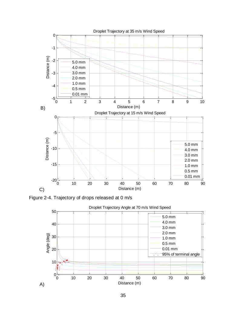
velocity. Figure 2-4 and Figure 2-5 depict drop trajectories for various drop diameters
and wind velocities; the trajectories were modeled assuming a steady flow of marked
velocity, and the drop drag coefficients and terminal velocities given by Gunn and
Kinzer (1949, model is explained in detail in Chapter 5). Figure 2-5 indicates that the
distance at which drops have achieved 95% of the theoretical trajectory angle—the

34
angle at which the horizontal component of the drop velocity is equal to the wind
velocity—is less than 55 m. Masters et al. (2010) reported a minimum mean and
standard deviation values of 126.2 ± 43.0 m, 74.4 ± 31.9 m, and 120.4 ± 54.4 m for 15
minute integral scales (at an elevation of 10 m) during Hurricanes Katrina, Rita, and
Wilma in 2005, respectively. Thus, assuming that the drop travels at the gradient wind
speed in tropical cyclones is valid.
As raindrops approach the building façade, higher wind speeds increase the
horizontal component of motion. With higher horizontal velocities, more drops are
susceptible to striking the building surface. Choi (1994) found that changing wind
velocity from 5.0 m/s to 30.0 m/s can increase LIF values up to 10 times for the top
quarter of a 4:1:1 ratio building. Therefore, increasing wind velocity will increase the
effect of all raindrop sizes on the building façade, particularly in the top quarters.
A)
0 1 2 3 4 5 6 7 8 9 10-5
-4
-3
-2
-1
0Droplet Trajectory at 70 m/s Wind Speed
Distance (m)
Dis
tance (
m)
5.0 mm
4.0 mm
3.0 mm
2.0 mm
1.0 mm
0.5 mm
0.01 mm
35
B)
C)
Figure 2-4. Trajectory of drops released at 0 m/s
A)
0 1 2 3 4 5 6 7 8 9 10-5
-4
-3
-2
-1
0Droplet Trajectory at 35 m/s Wind Speed
Distance (m)
Dis
tance (
m)
5.0 mm
4.0 mm
3.0 mm
2.0 mm
1.0 mm
0.5 mm
0.01 mm
0 10 20 30 40 50 60 70 80 90-20
-15
-10
-5
0Droplet Trajectory at 15 m/s Wind Speed
Distance (m)
Dis
tance (
m)
5.0 mm
4.0 mm
3.0 mm
2.0 mm
1.0 mm
0.5 mm
0.01 mm
0 10 20 30 40 50 60 70 80 900
10
20
30
40
50Droplet Trajectory Angle at 70 m/s Wind Speed
Distance (m)
Angle
(deg)
5.0 mm
4.0 mm
3.0 mm
2.0 mm
1.0 mm
0.5 mm
0.01 mm
95% of terminal angle

36
B)
C)
Figure 2-5. Distance required for the trajectory angle to reach 95% of the terminal angle
Terrain characteristics
Terrain characteristics affect the wetting of the building façade by changing the
characteristics of the flow upwind, particularly the mean wind speed and turbulence
intensity. Karagiozis et al. (1997) described the terrain characteristics affecting the flow
conditions upwind of the building façade; these characteristics range from ground
surface roughness dictating the global terrain exposures and overall flow conditions
(e.g., open, suburban, urban) to larger obstructions introducing local disturbances to the
0 10 20 30 40 50 60 70 80 900
10
20
30
40
50Droplet Trajectory Angle at 35 m/s Wind Speed
Distance (m)
Angle
(deg)
5.0 mm
4.0 mm
3.0 mm
2.0 mm
1.0 mm
0.5 mm
0.01 mm
95% of terminal angle
0 10 20 30 40 50 60 70 80 900
10
20
30
40
50Droplet Trajectory Angle at 15 m/s Wind Speed
Distance (m)
Angle
(deg)
5.0 mm
4.0 mm
3.0 mm
2.0 mm
1.0 mm
0.5 mm
0.01 mm
95% of terminal angle

37
upwind flow (e.g., close vicinity building obstruction). Significant distortions of the flow
pattern directly upwind of the building—resulting from the introduction of high turbulence
and mixing due to blockage and shielding effects of building obstructions at close
vicinity—causes the distribution of wetting on the building façade to deviate from what is
commonly expected (Choi, 1993). When no large obstructions are directly upwind, the
greatest effect to the wind flow pattern is due to the aerodynamic roughness length ( ).
The aerodynamic roughness length is defined as the height at which the mean velocity
is zero assuming a logarithmic velocity profile (Weber, 1999):
(2-21)
Where is the mean hourly wind velocity, is the height above the ground, and is
the friction velocity calculated per Weber (1999):
(2-22)
where is the eddy covariance between the longitudinal and vertical fluctuating
components. Surface roughness influences the boundary layer flow by decreasing the
mean wind speed and increasing the turbulence intensity as the elevation above the
ground decreases (Counihan, 1975). The change in mean wind speed and turbulence
will affect the temporal and spatial deposition of rain on the building façade (Blocken
and Carmeliet, 2002).
Building characteristics
Immersion of a building in a wind flow creates turbulence in the form of frontal
vortices, separations at the building edges/corners, corner streams, recirculation zones,
shear layers and the far wake (Bottema, 1993). The flow pattern is dependent on

38
upstream conditions, building orientation in the flow field, and building geometric shape.
When raindrops approach the bluff body the trajectories become complicated; the result
is non-uniform deposition on the building facade. Trajectories of small particles change
sharply; however, the higher inertia larger drops are less susceptible to local flow
disturbances and bluff body aerodynamic effects. As a result, the deposition contours
on the building façade of large drops are less affected than those corresponding to
smaller drops (Figure 2-6, after Blocken and Carmeliet, 2002).
Figure 2-6. Deposition of smaller drops left and larger drops right (arrows indicate
decreasing drop diameter)
The effect of varying building geometry, in particular width to height ratios,
changes the blockage effect on the wind flow. The number of drops diverted away from
the structure increases with higher aspect ratios. Choi (1994) experimentally verified
this phenomenon in an investigation of a narrow (H:W:D=4:1:1) building that exhibited
higher LIF values than a wider (H:W:D= 4:8:2) building (assuming similar drop sizes).
Modeling of Rain Deposition on the Building Façade
Semi-Empirical Models
Measurements from vectopluviometers and surface mounted instruments have
shown that is directly related to wind speed and horizontal rainfall intensity (Lacy,
1951; Hoppestad, 1955). This relationship has been the basis for multiple semi-

39
empirical models and has been used to derive regional WDR exposure from current
standard meteorological data provided by existing weather stations.
Hoppestad (1955) expressed the WDR intensity ( ) as a function of a WDR
coefficient ( , the inverse of drop terminal velocity), the wind velocity ( ), and the
horizontal rain intensity ( ). His work provided the basis for current semi-empirical
models.
(2-23)
Lacy (1965) used empirical relationships that express the median raindrop size as
a function of horizontal rainfall intensity and terminal velocity data to develop a single
WDR coefficient. The outcome was a refined equation that satisfies most WDR
scenarios (Lacey, 1965):
(2-24)
Empirical models have evolved to include the effect of the complex flow around
the building and output spatially varying rain deposition rates. Two of the most common
models are the Straube and Burnett (2000) model and the British Standard BS EN ISO
15927-3 (2009). Both models implement:
(2-25)
where is the WDR coefficient dependent on location on building and is the angle
between the wind direction and the perpendicular of the wall surface. A comprehensive
comparison of these methods performed by Blocken et al. (2010) found that while the
ISO model is more accurate than the Straube and Burnett model, neither accurately
model the blockage effect of the tested buildings.

40
For the purpose of this study, wetting rates were estimated in accordance with the
ISO model (BS EN ISO 15927-3:2009):
(2-26)
Where is the rain intensity reaching the building façade, is the roughness
coefficient representative of roughness of the terrain upwind of a wall (conservatively
assumed to be one), is the topography coefficient that accounts for wind speed up
over isolated hills and escarpments (conservatively assumed to be one), is the
obstruction coefficient that accounts for obstructions (e.g. buildings, fences, trees, etc.)
close to and upwind of building façade (conservatively assumed to be one), and is
the wall factor which is calculated as the ratio of water reaching the building façade to
the quantity passing through an equivalent unobstructed space (conservatively
assumed to be four, according to Table 4 in the BS EN ISO 15927-3:2009).
Numerical Models
The work by Choi (1993; 1994) has remained the foundation for most modern
techniques. Choi (1993, 1994) proposed a method for calculating WDR deposition on
the building façade that includes: (1) calculating wind flow under steady state conditions
by solving the Navier-Stokes equations with the k-ε turbulence model, and (2)
calculating drop trajectories at every point for each raindrop size by iteratively solving
their equations of motion 2-27 through 2-29, and 2-19 through 2-20 calculating and
values at different locations of the building.
(2-27)

41
(2-28)
(2-29)
In the equations of motion (2-27 – 2-29) is mass of the drop, is radius, is the air
density, is the water density, is the air viscosity, , , and are along, across, and
vertical wind directions, respectively.
Blocken and Carmeliet (2002) extended this work by introducing a temporal
component to the wind flow and examining the spatial and temporal WDR deposition on
the facade of the VLIET (Flemish Impulse Programme for Energy Technology) test
building (Blocken and Carmeliet, 2002).
Full Scale Experiments
Experimental wind engineering research directed at WDR effects on buildings is
limited. Only a few projects have been conducted in the wind tunnel (Flower and
Lawson, 1972; Rayment and Hilton, 1977; Inculet and Surry, 1994) and at full-scale
(e.g., Salzano, 2009; Bitsumalak, 2009; Lopez et al., 2011).
Wind tunnel experiments have been used to characterize wetting patterns on the
façade of multiple scale models. Due their complexity and high cost, wind tunnel tests of
WDR have been limited. Major difficulties encountered during these experiments
include (1) short duration of tests to not saturate the water sensitive paper, (2) counting
and measurement of drops on the water sensitive paper was extremely labor intensive,
(3) large variability between tests as a result of short test durations, and (4) obtaining a
uniform rain distribution was difficult due to the small size of the scaled drops (Inculet
and Surry, 1994).

42
Currently there are few methods for full scale simulation of WDR. These methods
are primarily employed in the product approval process, at the state level, to ensure a
minimum water infiltration resistance of building components. The testing procedures
require the application of static and cyclic pressures while a constant wetting rate is
applied to the exterior of a singular building component; these tests do not directly
investigate the holistic behavior of the building envelope, rather the behavior of each
component in isolation. In response, research efforts by RDH Building Engineering
Limited (2002), Florida International University (Bitsuamlak et al., 2009), and the
University of Florida (Masters et al.,2008; Salzano et al., 2010; Lopez et al., 2011) to
simulate WDR on full scale structures have been undertaken.
RDH Building and Engineering Ltd. (2002) sought to identify the adequacy of
building codes, standards, testing protocols, and certification processes towards wind
driven rain resistance of fenestration. The study analyzed the performance of 113
laboratory and 127 field window specimens. Field specimens were subjected to a
constant impinging jet while a constant rain rate was applied. The research at the
University of Florida (Salzano et al., 2010; Lopez et al., 2011) expanded on the RDH
study by evaluating water penetration resistance of window/wall assemblies subjected
to wind loading calibrated to tropical cyclone field data collected by the Florida Coastal
Monitoring Program (FCMP).
This emerging sub-discipline will greatly benefit from new insights regarding the
physical simulation of WDR and can ultimately lead to improved performance evaluation
of the water penetration resistance of building products and systems.

43
Measurement of Wind-Driven Rain
Instrumentation
In the earliest studies, WDR measurements were made using directional
pluviometers (known as vectopluviometers) and wall mounted collection chambers.
Vectopluviometers are fixed instruments that obtain directional quantities of WDR in the
free-stream with four or eight compartments of similar size openings—each facing the
cardinal or cardinal and ordinal directions, respectively—and an additional compartment
facing the vertical direction (Lacy, 1951; Choi,1996). The implementation of
vectopluviometers in various research projects (cf. Blocken and Carmeliet, 2004) has
produced directional WDR data that has been used for the development of WDR maps
(Lacy,1965), as a tool for estimating WDR deposition on building façades, and as basis
for the assumption that the increases proportionally with wind speed and
(discussed in semi-empirical simulation methods).
In the obstructed flow, collection chambers are attached to the walls of buildings to
directly measures the quantity of WDR deposited on the façade. These instruments are
collection chambers, of multiple sizes, mounted flush to a wall with an attached
reservoir to collect the deposited rain (Straube et al., 1995). Although implementation of
these instruments facilitated research of the spatial variability of WDR on the building
surfaces and the effects of building aspect ratio, wind velocity, and horizontal rainfall
intensity, they are unable to measure the RSD and wind characteristics.
Modern precipitation measurement instruments more accurately determine the
characteristics of rain but have limitations. Measurement by radar can produce detailed
precipitation data for an extensive area from a single location; however, measurements
are taken at heights where the RSD can vary from the ground level RSD, and the RSD

44
is not directly measured. RSD determination by radar is based on reflectivity
relationships (Richter and Hagen, 1997; Schafer et al., 2002) for which discrepancies
have been investigated by Marshall et al. (1947), Wilson and Brandes (1979), and
Medlin et al. (2007).
Disdrometers can accurately measure ground level RSD data at temporal
resolutions that are useful for WDR research (Joss and Waldvogel, 1967; Loffler-Mang
and Joss, 2000). Impact and optical disdrometers are the two most commonly used rain
sensors. Impact disdrometers, such as the Joss and Waldvogel disdrometer, measure
the induced voltage from the displacement of an aluminum covered styrofoam sensor
(Joss and Waldvogel, 1967). The voltage is amplified, and the drop size is interpreted
by fitting the voltage to predetermined voltage ranges corresponding to drop diameters
(Sheppard, 1990). The Joss and Waldvogel disdrometer can measure drop sizes
between 0.3 mm and 5 mm with resolutions varying from 0.1 mm for small drops to 0.5
mm for larger drops. Inherent limitations of the instrument manifest in high wind
scenarios, because the measuring algorithm expects drops to be falling at terminal
velocity (Sheppard, 1990; Tokay et al., 2008; Tokay et al.,2003).
Optical disdrometers function by creating a light band and measuring the voltage
drop from a photodiode, or series of photodiodes, as a drop passes through the light
band and a fraction of the light is obstructed from the photodiode (Loffler-Mang and
Joss, 2000). These instruments are capable of higher temporal resolution
measurements due to the lack of a sensor head which requires time to return to its
original position. Optical disdrometers are also more accurate than impact disdrometers
in measuring particles less than 0.7mm (Loffler-Mang and Joss, 2000).

45
Limitations of optical disdrometers
Currently, optical disdrometers are the instrument of choice for measuring ground
level RSD; however, these instruments have limitations that must be considered. The
major limitations of optical disdrometers include fringe effects, coincident measurement
of multiple drops, splashing effects, and errors associated with high wind.
Fringe effects refer to the partial measurement of a drop’s diameter as the drop
grazes the sensitive area; thus, the drop is recorded as a having an incorrect smaller
diameter and travelling much faster than correctly measured drops. The error in velocity
measurement propagates to an incorrect sample volume calculation which leads to an
under-estimation of and among other precipitation characteristics (Grossklaus et
al., 1998).
Errors associated with the coincident crossing of multiple drops occur if the optical
disdrometer cannot discriminate between the light extinction from one or multiple drops.
When multiple small drops simultaneously cross the sensitive area, a singular large
drop is recorded travelling at the velocity of the smaller drops. Thus, the sample volume
is erroneously small and the incorrectly measured large drop has an exaggerated
contribution to the rain parameters including and (Grossklaus et al., 1998).
Splashing effects occur when drops strike the instrument, breakup, and the
smaller remnants that bounce off, travel through the sensitive area at a much slower
velocity than the terminal velocity (Tokay et al., 2001). The measured drops are not
characteristic of the precipitation event and thus contaminate the data. The slow velocity
results in a small sample volume and the splashed drops have an exaggerated
contribution to the rain parameters including and .

46
The errors associated with high wind manifest as the incorrect diameter and
velocity measurement due to the oblique trajectory of drops as they travel through the
sample area. As wind velocities increase, the trajectory of the drops becomes more
horizontal; thus, they remain in the sensitive area longer and, through their passage,
occupy more of the horizontally aligned light band, leading to larger sampled areas
(Loffler-Mang and Joss, 2000). Additionally, depending on the structure of the
disdrometer, the distortion of the wind around the sensitive area significantly affects the
trajectory of drops reducing the quantity of drops crossing the sensitive area (Nespor et
al., 2000).
Many attempts have been made to mitigate these effects (Donnadieu, 1980;
Hauser et al., 1984; Grossklaus et al., 1998; Nespor et al., 2000; Tokay et al., 2001).
Disdrometers have been developed with the capability of sensing drops at the edge of
the sampling area. Illingworth and Stevens (1987) and Grossklaus et al. (1998)
developed disdrometers that employed an annular sensitive area rather than a flat
sheet. With this advancement, drops that graze the sensitive area are characterized by
a single voltage reduction and are thus excluded from the data. Drop Measurement
Technologies implemented multiple photodiodes to measure the voltage drop across flat
light sheet in the design of their Precipitation Imaging Probe (instrument is discussed in
the next section). In this arrangement, when the outer most photodiodes sense a drop in
the sensitive area, the drop is excluded from data. Other researchers (Donnadieu, 1980;
Hauser et al., 1984; Tokay et al., 2001) mitigate the effect of fringe effects, coincident
measurement of multiple drops and splashing effects limitations by employing quality
control algorithms that filter data according to the measured drop velocities and whether

47
or not they fall within a velocity threshold based on the work done by Gunn and Kinzer
(1949). These quality control algorithms typically exclude less than 20% of the data
(Tokay et al., 2001) and yield realistic results. Errors associated with high wind speed,
are addressed with the same algorithms and the exclusion of the data above a certain
velocity threshold (Tokay et al., 2008); however, instruments employing an annular
sensitive area, such as the Illingworth and Stevens (1987) and the Institut fur
Meereskunde (IfM) disdrometer (Grossklaus et al., 1998) were designed for operation in
high wind, but are not commercially available and to the authors knowledge, have only
been employed on ships for rainfall measurement over open ocean.
The instrument platforms used in this research (described in Chapter 3), employed
an OTT PARSIVEL disdrometer (Loffler-Mang and Joss, 2000) and a Drop
Measurement Technologies Precipitation Imaging Probe capable of high resolution
measurements, reporting precipitation at ten and one second intervals, respectively.
The instruments are described in the following section.
Instrumentation Used In This Study
OTT PARSIVEL optical disdrometer
Loffler-Mang and Joss (2000) produced the PARSIVEL– an easy to handle,
robust, and low cost disdrometer– that lends the ability to implement a network of
disdrometers to investigate small-scale variability (Loffler-Mang and Joss, 2000). The
OTT PARSIVEL records the count, diameter, and velocity of hydrometeors that pass
through a 30 mm X 160mm X 1 mm laser field. It functions by focusing the laser on a
single photodiode at the receiving end and measuring the analog voltage output (Figure
2-7). As particles pass through the laser field they obstruct a band of light,
corresponding to their diameter, from arriving to the photodiode and lower the measured

48
voltage from the steady state 5 V. The voltage time history is inverted, amplified,
filtered, and the DC component is removed (Loffler-Mang and Joss, 2000) such that the
diameter of the particle is estimated from voltage drop (ΔV). The duration of light
absence (Δt), from when the particle enters and exits the laser band, is used to estimate
the particle velocity. Particle diameters and velocities are then binned into diameter and
velocity classes (Table 2-1 and Table 2-2), and digitally output as time sampled
matrices (Figure 2-8). The particle shapes are assumed to be symmetric in the
horizontal plane and have linearly varying axis ratios of 1 to 1.3 for diameters 1 mm to 5
mm, 1 (spherical) for diameters < 1 mm, and 1.3 for diameters > 5 mm.
Table 2-1. PARSIVEL diameter classes
Class Number Class Average (mm) Class Spread (mm)
1 0.062 0.125
2 0.187 0.125
3 0.312 0.125
4 0.437 0.125
5 0.562 0.125
6 0.687 0.125
7 0.812 0.125
8 0.937 0.125
9 1.062 0.125
10 1.187 0.125
11 1.375 0.250
12 1.625 0.250
13 1.875 0.250
14 2.125 0.250
15 2.375 0.250
16 2.750 0.500
17 3.250 0.500
18 3.750 0.500
19 4.250 0.500
20 4.750 0.500
21 5.500 1.000
22 6.500 1.000
23 7.500 1.000
24 8.500 1.000

49
Table 2-1. Continued
Class Number Class Average (mm) Class Spread (mm)
26 11.000 2.000 27 13.000 2.000
28 15.000 2.000
29 17.000 2.000
30 19.000 2.000
31 21.500 3.000
32 24.500 3.000
Table 2-2. PARSIVEL velocity classes
Class Number Class Average (m/s) Class Spread (m/s)
1 0.050 0.100
2 0.150 0.100
3 0.250 0.100
4 0.350 0.100
5 0.450 0.100
6 0.550 0.100
7 0.650 0.100
8 0.750 0.100
9 0.850 0.100
10 0.950 0.100
11 1.100 0.200
12 1.300 0.200
13 1.500 0.200
14 1.700 0.200
15 1.900 0.200
16 2.200 0.400
17 2.600 0.400
18 3.000 0.400
19 3.400 0.400
20 3.800 0.400
21 4.400 0.800
22 5.200 0.800
23 6.000 0.800
24 6.800 0.800
25 7.600 0.800
26 8.800 1.600
27 10.400 1.600
28 12.000 1.600
29 13.600 1.600
30 15.200 1.600
31 17.600 3.200
32 20.800 3.200

50
Figure 2-7. PARSIVEL drop diameter and velocity determination
PARSIVEL Output:
Class V Class D
1 2 3 4 5 6 7 … 32
1 0 0 0 0 0 0 0 0 0
2 0 0 0 0 0 0 0 0 0
3 0 0 5 0 0 0 0 0 0
4 0 0 0 0 0 0 0 0 0
5 0 0 0 0 0 0 0 0 0
6 0 0 0 0 0 0 4 0 0
7 0 0 0 0 0 0 0 0 0
… 0 0 0 0 0 0 0 0 0
32 0 0 0 0 0 0 0 0 0
Figure 2-8. PARSIVEL measurement and output
0.30 mm drops (class 3)
traveling 0.34 m/s (class 3)
0.70 mm drops (class 6)
traveling 0.6 m/s (class 7)

51
Droplet Measurement Technologies Precipitation Imaging Probe
The Droplet Measurement Technologies (DMT) Precipitation Imaging Probe (PIP)
is a 2-D optical disdrometer that functions in the same manner as the OTT PARSIVEL
but has a higher resolution due to the use of 64 photodiodes instead of one. It measures
and counts drop diameters with 0.1 mm resolution up to 6.2 mm in a sample area of
260.0 mm x 6.4 mm. The PIP does not measure drop velocity; it assumes that all drops
are moving at the wind velocity and thus requires a continuous wind velocity input.
Additionally, the PIP is intended to be mounted on aircraft and operated at flight speeds.
Thus, the sample area is smaller than the OTT PARSIVEL sample area leading to a
smaller sample volume.
Rain parameters for both disdrometers are calculated as follows:
(2-30)
(2-31)
(2-32)
(2-33)
(2-34)
(2-35)

52
(2-36)
The variables introduced in Equations 2-30 to 2-36 are defined as follows:
is the number of diameter drops
is the sample volume
is the depth of field of the instrument
is the width of the diode array
is the velocity of drop through the laser plane
is the sample time of the instrument
is the density of water
is the third moment as defined in (2-8
is the equivalent radar reflectivity
is the mean measured drop diameter
is the volume weighted mean drop diameter (Testud et al., 2001).
Summary
This chapter presented an overview of the WDR phenomenon, simulation
methodologies adopted by other researchers, and instruments used to measure
precipitation. Information of the disdrometers used in this research has been presented,
and their applicability for WDR measurement will be discussed in Chapter 3.

53
CHAPTER 3
DESIGN, PROTOTYPING, AND IMPLEMENTATION OF ARTICULATING RAIN
PARTICLE SIZE MEASUREMENT PLATFORMS
This chapter presents the development and implementation of novel instrument
platforms intended for characterizing the raindrop size distribution (RSD) in strong
winds. To the author’s knowledge, this is the first known effort to successfully reduce
wind induced errors associated with ground based disdrometers. Thus, the data
collected provides a new resource for the study of wind driven rain (WDR). This chapter
is organized into three sections. First, the motivation for the development of an
instrument platform which actively aligns the disdrometer perpendicular to the mean rain
direction is discussed. This section demonstrates that in the absence of wind (i.e., drops
travelling perpendicular to the sensitive area) measurements made by the PARSIVEL
disdrometer and measurements made using a laborious but highly accurate procedure,
the Oil Medium Test, are similar. This section also demonstrates the limitations of the
instrument in the presence of wind (i.e., drops travelling obliquely through the sensitive
area). Second, details of the WDR measurement system are presented. Finally, a
comparison of collocated stationary and actively aligned disdrometers (henceforth
referred to articulating instruments) is presented.
Motivation for the Development of an Articulating Instrument Platform
Optical disdrometers are the instrument of choice for quantifying RSDs; however,
due to the limitations of these instruments (discussed in Chapter 2), data recorded in
high winds are usually excluded (Tokay et al., 2008). Lack of high-quality data has left
questions regarding the character of WDR in high wind events. Griffiths (1975)
proposed that actively aligning a disdrometer parallel to the mean rain direction could
theoretically improve accuracy by showing that the sample volume of an articulating

54
sensor was greater than that of the sensor in the stationary, horizontally aligned,
configuration (the proof is shown in the Appendix). Bradley and Stow (1975) attempted
such an experiment but found that device was unmanageable in high wind, dripped
water into the sensitive area when tilted, and were not certain how to define a mean rain
direction. Since then, disdrometers and servomotor systems have become lighter,
easier to use, and less expensive. Thus, the author investigated the option of aligning
disdrometers to the mean rain direction by performing a series of laboratory tests
intended to reduce measurement errors associated with high wind speeds.
Raindrop Size Distribution Verification Using the Oil Medium Test
The Oil Medium Test was performed to demonstrate that when properly employed
(i.e. drops travelling perpendicular to the sample area), the PARSIVEL disdrometer
yields a reliable estimate of the RSD. The test was performed under ideal stagnant air
conditions where the RSDs recorded by the PARSIVEL were compared to RSDs
obtained from water drops collected in oil. The PIP was not used to calculate the
stagnant air RSD because the instrument requires continuous wind velocity feed back to
calculate the sample volume, rather than using the drop velocity.
Raindrop size distributions from drops collected in oil were calculated using a
morphological image processing algorithm (van den Boomgaard and van Balen, 1992;
Adams, 1993; Jones and Soille, 1996). The experimental setup included setting a single
nozzle 3.0 m above a collection dish containing the oil medium, setting the water
pressures, and exposing the collection dish to five seconds of continuous spray. A 20
megapixel, RAW format, picture of the collection dish was then immediately taken using
a Canon ® EOS 5D Mark II Digital SLR Camera with a Canon ® Telephoto EF 100mm
f/2.8 USM macro lens with the ISO set to 320, relative aperture set to 7.1, white balance

55
set to 6300K, and shutter speed set to 1/10 sec. To maximize the contrast between the
dish and drops, a blue dye (Cole Parmer #00298-18) was used. Care was also taken in
the selection of the oil medium, by selecting a clear mineral oil with a specific density
similar to water. The oil properties prevented distortion of the shape of the drops and
essentially captured the drops as they were when falling freely. The photographs were
filtered using Adobe® Photoshop® to obtain a high contrast black and white image. The
black and white images were then analyzed by the morphological image processing
algorithm to obtain the size of each drop by scaling the pixel counts (Figure 3-1). The
data was then binned using PIP specifications and an RSD was obtained.
In this experiment, six measurements were taken by the PARSIVEL and images of
15 oil medium tests were processed by the morphological image processing algorithm,
yielding the RSDs shown in Figure 3-2. In general the PARSIVEL measured a smaller
number of drops larger than 2 mm in diameter; however, the source of the difference is
unclear and for practical purposes the two RSDs are reasonably similar.
Figure 3-1. Sample picture from morphological image processing algorithm
1.00 mm
10x Magnification
Reference1.0 cm x 1.0
cmArea
0.15 mm
30x Magnification

56
Figure 3-2. Comparison of different raindrop size distribution measurement techniques
Bearing Drop Test
The bearing drop test was performed to replicate the effect of high wind speeds on
stationary PARSIVEL measurements by dropping 20 high tolerance steel bearings(1
mm, 2 mm, and 3 mm) from 6.1 m height (Figure 3-3) through the laser plane at multiple
elevation angles (90°, 80°, 70°, 60°, 50°, 45°, 40°). The results of this test are found in
Figure 3-4 and Figure 3-5. The figures demonstrate that the PARSIVEL correctly
measured the bearing diameters regardless of trajectory angle; however, at 50° or
lower, incorrect measurements of the velocity indicate that the measured velocity is
dependent of the trajectory angle and can deviate significantly from the theoretical
velocity. Small diameter measurements (much less than 1mm) are assumed to be
margin fallers. Similar results were observed by Friedrich et. al (2011) in which 2-6 mm
drops were recorded as having reduced fall velocities when travelling obliquely through
the sensitive area; however, at more extreme elevation angles, unrealistically high drop
diameters were recorded indicating that incorrect drop diameter measurements may
0 0.5 1 1.5 2 2.5 3 3.5 410
-2
100
102
104
106
Diameter (mm)
Co
nce
ntr
atio
n (
mm
-1 m
-3)
PARSIVEL RSDs
Mean PARSIVEL RSD
RSDs from Algorithm
Mean RSD from Algorithm

57
occur high wind speeds, even though it was not observed in this experiment. Thus, the
observed results may not be representative of every natural scenario.
Figure 3-3. Angled trajectory experiment configuration
To relate the trajectory angle to specific wind speeds, 3-1 was used (Based on the
Lacy 1965 Equation):
(3-1)
where is the terminal velocity of the drop and is the wind velocity. Table 3-1
demonstrates the sensitivity of the trajectory angle to drop diameter and wind velocity.
The table indicates that at 10 m/s wind speeds, trajectory angles of the majority of
the drops (< 5 mm) will be far below the 50° threshold. This implies that at wind speeds
of 10 m/s drop velocities can be underestimated by at least 40%, yielding incorrect RSD
measurements. The effect of oblique trajectory angles was further investigated in winds
generated by the UF Windstorm Simulator.
Table 3-1. Trajectory angles of multiple diameter drops in multiple wind speeds
Drop Diameter
(mm) Vt(m/s) U = 5 m/s U = 10 m/s U = 15 m/s U = 20 m/s
1.0 4.0 38.9° 21.9° 15.0° 11.4°
2.0 6.5 52.4° 33.0° 23.4° 18.0°
3.0 8.1 58.2° 38.9° 28.3° 21.9°
4.0 8.8 60.5° 41.4° 30.5° 23.8°
5.0 9.1 61.2° 42.3° 31.2° 24.4°
θ
Bearing
Direction
6.1m
Drop
Height
Laser
Band

58
Figure 3-4. PARSIVEL measured diameters at multiple trajectory angles
0 1 2 3 405
101 mm Bearing measured at 90 deg
Measured Diameter (mm)
Co
un
t
0 1 2 3 405
101 mm Bearing measured at 80 deg
Measured Diameter (mm)
Co
un
t
0 1 2 3 405
101 mm Bearing measured at 70 deg
Measured Diameter (mm)
Co
un
t
0 1 2 3 40
1020
1 mm Bearing measured at 60 deg
Measured Diameter (mm)
Co
un
t
0 1 2 3 405
101 mm Bearing measured at 50 deg
Measured Diameter (mm)
Co
un
t
0 1 2 3 405
101 mm Bearing measured at 45 deg
Measured Diameter (mm)
Co
un
t
0 1 2 3 405
101 mm Bearing measured at 40 deg
Measured Diameter (mm)
Co
un
t
0 1 2 3 405
102 mm Bearing measured at 90 deg
Measured Diameter (mm)
Co
un
t
0 1 2 3 405
102 mm Bearing measured at 80 deg
Measured Diameter (mm)
Co
un
t
0 1 2 3 405
102 mm Bearing measured at 70 deg
Measured Diameter (mm)
Co
un
t0 1 2 3 4
05
102 mm Bearing measured at 60 deg
Measured Diameter (mm)
Co
un
t
0 1 2 3 405
102 mm Bearing measured at 50 deg
Measured Diameter (mm)
Co
un
t
0 1 2 3 40
52 mm Bearing measured at 45 deg
Measured Diameter (mm)
Co
un
t
0 1 2 3 405
102 mm Bearing measured at 40 deg
Measured Diameter (mm)
Co
un
t
0 1 2 3 40
1020
3 mm Bearing measured at 90 deg
Measured Diameter (mm)
Co
un
t
0 1 2 3 405
103 mm Bearing measured at 80 deg
Measured Diameter (mm)
Co
un
t
0 1 2 3 405
103 mm Bearing measured at 70 deg
Measured Diameter (mm)
Co
un
t
0 1 2 3 405
103 mm Bearing measured at 60 deg
Measured Diameter (mm)
Co
un
t
0 1 2 3 405
103 mm Bearing measured at 50 deg
Measured Diameter (mm)
Co
un
t
0 1 2 3 405
103 mm Bearing measured at 45 deg
Measured Diameter (mm)
Co
un
t
0 1 2 3 405
103 mm Bearing measured at 40 deg
Measured Diameter (mm)
Co
un
t

59
Figure 3-5. PARSIVEL measured velocities at multiple trajectory angles (dashed line indicates theoretical velocity)
0 5 100
1020
1 mm Bearing measured at 90 deg
Measured Velocity (m/s)
Co
un
t
0 5 100
1020
1 mm Bearing measured at 80 deg
Measured Velocity (m/s)
Co
un
t
0 5 100
1020
1 mm Bearing measured at 70 deg
Measured Velocity (m/s)
Co
un
t
0 5 100
1020
1 mm Bearing measured at 60 deg
Measured Velocity (m/s)
Co
un
t
0 5 100
1020
1 mm Bearing measured at 50 deg
Measured Velocity (m/s)
Co
un
t
0 5 100
1020
1 mm Bearing measured at 45 deg
Measured Velocity (m/s)
Co
un
t
0 5 100
1020
1 mm Bearing measured at 40 deg
Measured Velocity (m/s)
Co
un
t
0 5 100
1020
2 mm Bearing measured at 90 deg
Measured Velocity (m/s)
Co
un
t
0 5 100
1020
2 mm Bearing measured at 80 deg
Measured Velocity (m/s)
Co
un
t
0 5 100
1020
2 mm Bearing measured at 70 deg
Measured Velocity (m/s)
Co
un
t
0 5 100
1020
2 mm Bearing measured at 60 deg
Measured Velocity (m/s)
Co
un
t
0 5 100
1020
2 mm Bearing measured at 50 deg
Measured Velocity (m/s)
Co
un
t
0 5 100
1020
2 mm Bearing measured at 45 deg
Measured Velocity (m/s)
Co
un
t
0 5 100
1020
2 mm Bearing measured at 40 deg
Measured Velocity (m/s)
Co
un
t
0 5 100
1020
3 mm Bearing measured at 90 deg
Measured Velocity (m/s)
Co
un
t
0 5 100
1020
3 mm Bearing measured at 80 deg
Measured Velocity (m/s)
Co
un
t
0 5 100
1020
3 mm Bearing measured at 70 deg
Measured Velocity (m/s)
Co
un
t
0 5 100
1020
3 mm Bearing measured at 60 deg
Measured Velocity (m/s)
Co
un
t
0 5 100
1020
3 mm Bearing measured at 50 deg
Measured Velocity (m/s)
Co
un
t
0 5 100
1020
3 mm Bearing measured at 45 deg
Measured Velocity (m/s)
Co
un
t
0 5 100
1020
3 mm Bearing measured at 40 deg
Measured Velocity (m/s)C
ou
nt

60
Instrument Performance in High Wind Speeds
The option of orienting the PARSIVEL into the mean rain direction was further
investigated by recording the RSD with PARSIVELs oriented at 0.0°, 22.5°, and 45.0°
elevation angles; a nozzle array operating at 68.9, 103.4, and 137.9 kPa water
pressures (corresponding to approximately 400, 475, and 550 mm/hr); and steady wind
velocities of 8.9, 17.9, and 35.8 m/s. Three PARSIVEL measurements were taken for
each test configuration listed in Table 3.2. The PIP measurements were used as the
reference measurement, given that this instrument is intended to be used in high wind
speeds and is more accurate. The instruments were mounted on a gantry system
shown in Figure 3-6. The PARSIVEL disdrometer exhibited no noticeable inaccuracies
due to increasing rainfall intensities; however, inaccuracies were observed at the high
wind velocities (Figure 3-7). As expected, at high wind velocities, the instruments
oriented at 22.5° and 45.0° recorded drops travelling slower than the instrument at 0.0°
(Figure 3-8). The incorrectly measured velocities decrease the sample volume over
which the RSDs are calculated; therefore, data from these instruments yield incorrect
RSDs (as shown in Figure 3-7). This experiment also demonstrated that the PARSIVEL
measured a smaller number of large drops (larger than 2 mm) when compared to the
PIP; however, for practical purposes, when the PARSIVEL is properly employed, the
measured RSD is similar to that of the PIP. These results demonstrate that, as Griffiths
(1974) proposed, aligning the disdrometer with the mean rain direction improves
accuracy. Thus, a novel approach was taken to continuously align the disdrometer with
the mean rain vector; described in the following section.

61
Table 3-2. Steady wind test matrix
Test Number
Angle (deg) Wind Speed (m/s) Water Pressure (kPa)
0.0 22.5 45.0 8.9 17.9 35.8 69 103 138
1 • • • •
•
2 • • • •
•
3 • • • •
•
4 • • •
•
•
5 • • •
•
•
6 • • •
•
•
7 • • •
• •
8 • • •
•
•
9 • • •
•
•
Figure 3-6. Steady wind instrument configuration (photo courtesy of author)

62
Figure 3-7. PARSIVEL measured raindrop size distributions for the tests in steady wind flow
0 2 4 610
-2
100
102
104
106
Diameter (mm)
U =
8.9
m/s
Co
nce
ntr
atio
n (
mm
-1m
-3) R
wdr ~ 400 mm/hr
0 2 4 610
-2
100
102
104
106
Diameter (mm)
Co
nce
ntr
atio
n (
mm
-1m
-3)
Measured RSDR
wdr ~ 475 mm/hr
0 2 4 610
-2
100
102
104
106
Diameter (mm)
Co
nce
ntr
atio
n (
mm
-1m
-3) R
wdr ~ 550 mm/hr
0 2 4 610
-2
100
102
104
106
Diameter (mm)
U =
17
.9 m
/s
Co
nce
ntr
atio
n (
mm
-1m
-3)
0 2 4 610
-2
100
102
104
106
Diameter (mm)
U =
35
.8 m
/s
Co
nce
ntr
atio
n (
mm
-1m
-3)
0 2 4 610
-2
100
102
104
106
Diameter (mm)
Co
nce
ntr
atio
n (
mm
-1m
-3)
0 2 4 610
-2
100
102
104
106
Diameter (mm)
Co
nce
ntr
atio
n (
mm
-1m
-3)
0 2 4 610
-2
100
102
104
106
Diameter (mm)
Co
nce
ntr
atio
n (
mm
-1m
-3)
0 2 4 610
-2
100
102
104
106
Diameter (mm)
Co
nce
ntr
atio
n (
mm
-1m
-3)
0 deg 22.5 deg 45 deg PIP

63
Figure 3-8. PARSIVEL measured drop diameters and velocities for the tests in steady wind flow
Diameter (mm)
8.9
m/s
Ve
locity (
m/s
)0 deg
0 1 2 30
5
10
15
0
100
200
300
400
500
Diameter (mm)
Ve
locity (
m/s
)
BETE WL1-1/2 Nozzle Grid at ~ 400 mm/hr22.5 deg
0 1 2 30
5
10
15
Diameter (mm)
Ve
locity (
m/s
)
45 deg
0 1 2 30
5
10
15
Diameter (mm)
17
.9 m
/sV
elo
city (
m/s
)
0 1 2 30
5
10
15
Diameter (mm)
35
.8 m
/sV
elo
city (
m/s
)
0 1 2 30
5
10
15
0
100
200
300
400
500
0
100
200
300
400
500
0
100
200
300
400
500
Diameter (mm)
Ve
locity (
m/s
)
0 1 2 30
5
10
15
0
100
200
300
400
500
Diameter (mm)
Ve
locity (
m/s
)
0 1 2 30
5
10
15
0
100
200
300
400
500
0
100
200
300
400
500
Diameter (mm)
Ve
locity (
m/s
)
0 1 2 30
5
10
15
0
100
200
300
400
500
Diameter (mm)
Ve
locity (
m/s
)
0 1 2 30
5
10
15
0
100
200
300
400
500

64
Articulating Instrumentation Platforms
An instrumentation platform was designed, prototyped, and implemented in
supercell thunderstorms and Atlantic hurricanes to supplement FCMP weather station
T-3 which contains a similar actively controlled system that aligns the PIP to the mean
rain direction. The platforms are capable of high temporal resolution measurements of
wind and rain. This section describes the components of the articulating instrumentation
platform (illustrated in Figure 3-9), its operation, the quality control algorithm, and a
description of FCMP weather station T-3.
Articulating Instrumentation Platform Components
The articulating instrument platform consists of the following six components,
which are discussed in the following subsections:
1. An OTT PARSIVEL optical disdrometer (described in Chapter 2)
2. An RM Young Model 851062D Sonic Anemometer
3. An articulating instrument support structure that is driven by two IMS M-17 stepper motors with an integrated controller and encoder (Model MDI4MRQ17C4-EQ-G1C3)
4. A Labview 8.5 software data acquisition system, which consists of a laptop computer connected to a four port RS-485 National Instruments serial interface
(Model No. NI USB-485/4)
5. A battery array of 12V 35 AH Power Sonic (PS-12350 NB) batteries to supply
power to the instruments
6. A substructure to provide lateral stability and to transfer the gravity and wind
loads to the ground

65
Figure 3-9. Articulating instrument platform
RM Young sonic anemometer
Wind velocity and direction are measured by an RM Young Model 85106Sonic
Anemometer. A sonic anemometer was chosen for its compact size, lack of moving
parts, and superior performance in low winds when compared to a mechanical (plate or
cup) anemometer. Mechanical anemometers have a distance constant on the order of
2-10m, and for practical purposes, the distance constant of sonic anemometers is
considered to be zero. Sonic instruments operate by measuring the time it takes for
ultrasonic pulses to travel between four transducers. The 85106 is capable of
measuring wind velocities up to 70 m/s ±0.1 m/s and direction 0° to 360° ± 2° at 4 Hz.
Data are output on independent analog channels (0-5V) and on a digital channel to the
motion control systems and computer, respectively.

66
Articulating support structure
The instrumentation array is continuously rotated by two Intelligent Motion
Systems (IMS M17Plus) motion control systems (stepper motor, driver and controller) to
align the optical disdrometer with the ten second mean rain vector (Figure 3-10). The
motor controllers are programmed in a proprietary programming language (MCode) to
read the 0-5V analog signal for wind speed and direction from the sonic anemometer.
The voltage is interpreted as the angle required to rotate the instrument. The elevation
equations were based on the Lacy relationship (1970, Equation 2.6) for a 1.2 mm
particle.
Figure 3-10. Articulating instrument platform automation
To ensure that the platform will resist high wind loads it was designed to withstand
the expected peak gust wind load caused by a minimal Category 5 tropical cyclone
( ), as defined by the Saffir-Simpson Scale (Simpson 1974, Simpson and
Wind/Rain Direction
Parsivel will slowly rotate into alignment with the mean rain vector
Instrument array will slowly rotate into alignment with the mean wind velocity vector

67
Riehl 1984). The structural system was idealized as a system of cylinders acted on by
drag forces computed using:
(3-2)
(3-3)
Where is air density, is air velocity, is cylinder diameter, is cylinder length, is
drag coefficient, and is kinematic viscosity. Drag coefficients were found using Figure
3-11 and (3-3 for a given Reynolds number, . The moment at was found
to be while the moment required to overturn the instrument was found to be
.
Figure 3-11. Drag coefficient of a cylinder dependant of Reynolds number of flow (Adapted from R Panton, Incompressible Flow 3rd ed.)
Data acquisition system
Data from the disdrometer, anemometer, and internal encoders on the stepper
motors are transmitted digitally via RS-485 lines and recorded on a laptop computer
running a custom written data logger operating on the National Instruments LabView 8.5
platform. The control and data diagram is shown in Figure 3-12. The system is also

68
capable of streaming summary data via a cellular connection, should future needs
warrant an upgrade.
Figure 3-12. Instrument platform control and data diagram
Power
The system was designed to run on battery power for a period of time sufficient to
record the passage of a tropical cyclone. With capacity of each, three Power
Sonic (PS-12350 NB) batteries will supply the mean amperage draw of 4 amps for over
24 hrs.
Substructure
The instrument platform is placed above a heavy duty tripod with wide set legs to
maximize the overturn capacity. At the base of each tripod leg a 609.6 mm (24 in) steel
stake is embedded in the ground. A guide wire can also be used to secure the system
to an earth screw placed below the center of gravity. Once the tripod is secured, the
Digita
l Signa
lE
levatio
n A
ngle
Control Algorithm
Win
d S
pee
dA
nal
og
0-1
0V
Win
d D
irec
tio
nA
nal
og
0-1
0V
Data Logger/ National Instruments Labview 8.5
Software
Digital SignalWind Data
Digital Sign
al
Azim
uth
Digital Sign
al
Rain
Da
ta
Elevation Angle
Stepper Motor
Azimuth
Stepper Motor

69
data and power cables are connected to ports on the enclosure box and the software is
set to operate.
The use of a collapsible tripod that assembles in the field permitted the system’s
portability and rapid deployment. During the VORTEX2 deployment the instrument was
assembled, operational, and recording in less than three minutes. Portability of the
instrument array is required to allow the set up of multiple systems in storm paths
expected to contain the most rain. Rapid deployment is crucial since weather conditions
can quickly worsen and pose unsafe conditions for the operator.
Portable Instrument Platform Operation
System operation, as illustrated in Figure 3-12, begins with anemometer
measurement of wind velocity and direction. The anemometer outputs the 0-5 V analog
signals to the motion control systems which continuously calculate the 10 second
average. The azimuth motion control system interprets the deviation from 2.5V – the
voltage corresponding to a wind direction perpendicular to the instrumentation platform
–as a number of steps for the stepper motors to rotate. When the motion is complete
the control system re-samples and rotates. This process continuously aligns the
instrument array perpendicular to the wind direction. The elevation motion control
system interprets the analog signal and assigns a number of steps to rotate based on
the programmed formula relating wind velocity to drop trajectory (Lacy 1970, Equation
2-6 for 1.2 mm particle). This aligns the disdrometer to the mean rain vector. The motion
control systems digitally output their location, via RS-485 channels, at the completion of
each prescribed rotation. The disdrometer and anemometer digitally output their
measurements via RS-485 channels every 10 seconds and at 14 Hz, respectively. The

70
data acquisition system records the measurements from all of the instruments, as
previously described.
Quality Control Algorithm
To mitigate fringe effects, coincident measurement of multiple drops, and
splashing effects (described in Chapter 2) a quality control algorithm was employed.
The algorithm filters data that fall below 50% of the expected terminal velocity (Gunn
and Kinzer, 1949) and above the maximum expected velocity ( ), defined as the
resultant of the terminal velocity ( ) and wind speed ( ) plus one standard deviation.
Additionally, the algorithm only considers data above 5 mm/hr and drops smaller than
10 mm (Figure 3-13). The algorithm ensures that drops that graze the sensitive area
(characterized by small measured diameter at a high speed), multiple drops
(characterized by a large drop at low speed), and drops resulting from splashing
(characterized by small drops at low speed) are mostly excluded from the analyzed
dataset.
A)
0 5 10 15 200
2
4
6
8
10
12
14
16
18
20
Diameter (mm/hr)
Ve
locity (
m/s
)
U = 0 m/s
Considered D-V Combinations
VT
VR
Observed

71
B)
Figure 3-13. Quality control filter at U = 0 m/s and U = 10 m/s
Description of Weather Station T-3
The FCMP portable weather stations are 10 m structural steel lattice towers
mounted on dual axel trailers for rapid deployment (Poss, 2000). The tower system and
outriggers unfold and are operational in minutes. The stations are equipped with three
fixed axis anemometers (RM Young 27106R) at 5 m and 10 m to measure the 3D wind
speed and direction. At the 10 m location is an additional anemometer (RM Young
05103V) that measures the resultant of the lateral and longitudinal component of wind
and serves as a redundant measurement (Balderrama et al., 2011). FCMP tower T-3 is
the only of the six weather stations that is outfitted for precipitation measurement.
Rainfall measurements are made by a DMT PIP (described in Chapter 2) at a 3 m
height. In order for the PIP operate correctly, the laser plane must be oriented
perpendicular to the rain vector. To achieve this, the PIP is mounted on an automated
0 5 10 15 200
2
4
6
8
10
12
14
16
18
20
Diameter (mm/hr)
Velo
city (
m/s
)
U = 10 m/s
Considered D-V Combinations
VT
VR
Observed

72
turret that continuously aligns the disdrometer (Figure 3-14). The azimuth angle of the
turret is actively controlled by a positioning system that continuously samples the gill
anemometers at 5.0 m. The elevation angle is governed by the elevation equations
derived from work by Lacy (1970, Equation 2.6 for 1.2 mm particle). Wind and rain are
reported at 10 Hz and 1Hz, respectively. Results from data gathered by both platforms
during supercell thunderstorms and Atlantic hurricanes are discussed at length in the
Chapter 4.
Figure 3-14. T-3 Precipitation Imaging Probe turret system and Gill anemometers at 5.0
m (photo courtesy of author)

73
Comparison of Collocated Stationary and Articulating Instruments in a Supercell Thunderstorm
Data from a supercell thunderstorm were collected with collocated stationary and
articulating instrumentation platforms (Figure 1-1). A difference in accuracy was
confirmed in measurements of the RSDs between the two instrumentation platforms.
The stationary instrumentation platform measured unrealistic large number
concentrations of drop diameters larger than 4 mm (Figure 3-15 top) in high wind
velocities (> 10 m/s). This phenomenon was not apparent in the articulating instrument
platforms (Figure 3-15 center). The unrealistic large number concentrations were found
to be attributable to erroneously low measured drop velocities (generally less than 2
m/s). Incorrect measurements of the RSD subsequently lead to incorrect estimates of all
rainfall parameters in the stationary instrumentation platforms (rainfall intensity - Figure
3-16 and reflectivity - Figure 3-17). The articulating instrument platform did not exhibit
similar jumps in the data, indicating reliable measurements.
A) 0 0.1 0.2 0.3 0.4 0.5 0.6 0.7 0.8 0.9 1
0
0.2
0.4
0.6
0.8
1
0 0.1 0.2 0.3 0.4 0.5 0.6 0.7 0.8 0.9 10
0.2
0.4
0.6
0.8
1
Time
Dro
p D
iam
ete
r (m
m)
Measured RSD on Jun 10, 2010
01:17Z 01:25Z 01:33Z 01:41Z 01:49Z 01:58Z
1
2
3
4
5
6
7
8
10-1
100
101
102
103

74
B)
C)
Figure 3-15. Measured raindrop size distribution by stationary instrumentations (A) and articulating instrumentation (B)
Figure 3-16. Comparison of rainfall intensities measured by stationary and articulating instrument platforms
0 0.1 0.2 0.3 0.4 0.5 0.6 0.7 0.8 0.9 10
0.2
0.4
0.6
0.8
1
0 0.1 0.2 0.3 0.4 0.5 0.6 0.7 0.8 0.9 10
0.2
0.4
0.6
0.8
1
Time
Dro
p D
iam
ete
r (m
m)
Measured RSD on Jun 10, 2010
01:17Z 01:25Z 01:33Z 01:41Z 01:49Z 01:58Z
1
2
3
4
5
6
7
8
10-1
100
101
102
103
01:17Z 01:25Z 01:33Z 01:41Z 01:49Z 01:58Z0
5
10
15
Time
Win
d S
pe
ed
(m/s
)
01:17Z 01:25Z 01:33Z 01:41Z 01:49Z 01:58Z0
200
400
600
800
1000
1200
Time
Ra
infa
ll r
ate
(mm
/hr)
Measured Rainfall Rate Comparison of Data Collected on Jun 10, 2010
Articulating Instrument
Stationary Instrument

75
Figure 3-17. Comparison of estimated reflectivity by stationary and articulating
instrument platforms
Summary
This chapter presented the known inaccuracies in RSD characterization caused by
strong winds. As a result, an articulating instrument platform was designed, prototyped,
and evaluated in the field. The articulating instrument platform did not exhibit the errors
observed in the stationary instrument; thus, the approach taken to measure WDR in
strong winds was validated. The next chapter presents the analysis and results of data
collected during the VORTEX2 and FCMP field campaigns.
01:17Z 01:25Z 01:33Z 01:41Z 01:49Z 01:58Z0
20
40
60
80
100
Time
Re
fle
ctivity(d
BZ
)
Reflectivity Comparison of Data Collected on Jun 10, 2010
Articulating Instrument
Stationary Instrument

76
CHAPTER 4
CHARACTERIZATION OF WIND-DRIVEN RAIN IN STRONG WINDS
This chapter addresses field research conducted during the Verification of the
Origins of Rotation in Tornadoes Experiment 2 (VORTEX2) and Florida Coastal
Monitoring Program (FCMP) field deployments during Hurricanes Ike (2009) and Irene
(2011). This portion of the research analyzed the wind-driven rain (WDR) data collected
in extreme events. The goals were to:
1. Determine the effect of wind on raindrop size distribution (RSD)
2. Determine if the RSD models used in computational wind engineering are appropriate for modeling the rain deposition rate on buildings during a design-
level wind event
3. Characterize the peak to mean ratio of rainfall intensity and determine the impact
on design for water penetration resistance
4. Investigate if the precipitation algorithm in the radar product generator used by
the National Weather Service (NWS) Weather Surveillance Radar exhibits any biases that manifest in extreme wind events
This chapter is organized into six sections: (1) a description of the field research
programs, (2) the effect of wind on the drop diameter, (3) the effect of wind on the RSD,
(4) comparison of RSD models to RSDs measured in multiple wind velocities, (5)
calculation of the peak to mean ratios of rainfall intensity ( ), and (6) comparison of
measured rain data to WSR-88D data.
Field Research Programs
Verification of the Origins of Rotation in Tornadoes Experiment 2 (VORTEX2)
Overview
The Verification of the Origins of Rotation in Tornadoes Experiment 2 (VORTEX2)
Project—a continuation of the original VORTEX project described by Rasmussen et al.
(1994)—was an interdisciplinary multi-agency effort to investigate tornado genesis,

77
dynamics, kinematics, demise, supercell near-ground wind field, and how the
environment regulates storm structure. VORTEX2 assets included 10 mobile radars, 12
mobile mesonet instrumented vehicles, and 38 deployable instruments including,
disdrometers, surface level wind measurement stations, weather balloon launching
vans, and unmanned aircraft that were deployed in the projected path of supercell
thunderstorms minutes prior to their arrival. Data collected will assist scientists in better
understanding tornadic behavior and improving tornado forecasting.
Deployment details
As part of VORTEX2, a disdrometer team was tasked with the repeated
deployment of eight instrument stations (articulating and stationary) for the collection of
RSD data. During each day of field collection, team leaders would determine locations
exhibiting favorable conditions for storm formation. The teams would then mobilize and
target a supercell thunderstorm that exhibited potential for tornadic activity. The
instruments were deployed perpendicular to storm motion in the path of the hook
appendage minutes before the approaching storm passed through the area (Figure
4-1). Spacing between instrument stations was 0.5 km to 2 km based on storm velocity
and the projected storm path. Upon storm passage instruments were collected and
relocated in the projected path of the same storm in the same configuration. A total of
144 measurements were collected during 32 supercell thunderstorms with eight
instrument platforms (Table 4-1) in the states shown in Figure 4-2 through the period of
May 1 to June 15, 2010. Data admitted for analysis consists of the 25 observations
collected with the articulating instrumentation platforms (denoted by * in Table 4-1); the
observations consist of 16 Hz wind velocity and 0.1 Hz rain time histories (see Chapter

78
3). The data was collected over open terrain, clear of any obstructions, and at a
sufficient distance from roads to minimize errors associated with vehicle spray.
Table 4-1. Verification of the rigins of Rotation in Tornadoes Experiment 2 deployment
details
Date
Time (UTC,
HHMM) Location Instrument Platforms
06-May 0010-0058 Oberlin, KS CU1 CU2
10-May 2212-2303 Chandler, OK CU1 CU2
*11-May 0128-0240 Clinton, OK CU1 CU2 UF1* UF4 UF5 UF6 UF7
12-May 2350-0100 Willow, OK CU1 UF4 UF5 UF6 UF7
14-May 1850-1900 Odessa, TX UF7
14-May 1934-2030 Odessa, TX CU1 UF4 UF5 UF6 UF7
14-May 2127-2230 Odessa, TX CU1 UF4 UF5 UF6 UF7
15-May 2330-0800 Artesia, NM CU1 UF4 UF5 UF6 UF7
*17-May 2150-2345 Artesia, NM CU1 UF1* UF4 UF5 UF6 UF7
*18-May 2240-0300 Dumas, TX CU1 UF1* UF4 UF5 UF6 UF7
19-May 2029-2145 Watonga, OK CU1
*21-May 0035-0123 Mitchell, NE CU1 UF1* UF4 UF5 UF6 UF7
*24-May 2123-2205 Ogallala, NE CU1 UF1* UF4
24-May 2230-2300 Ogallala, NE CU1 UF4 UF5 UF6
25-May 0005-0100 Ogallala, NE CU1 UF5 UF6 UF7
*29-May 0015-0140 Thedford, NE CU1 UF1*UF3* UF4 UF5 UF6 UF7
*02-Jun 2255-2355 Benkelman, NE CU1 UF1*UF3* UF5 UF6
*03-Jun 0020-0100 Wagner, SD UF1*UF3* UF5 UF6
*05-Jun 2330-0010 Des Moines, IA CU1 UF1*UF3* UF5 UF6
*06-Jun 2220-0210 Ogallala, NE CU1 UF1* UF5 UF6
*06-Jun 0110-0210 Ogallala, NE CU1 UF1* UF5 UF6
*07-Jun 2335-0030 Scottsbluff, NE CU1 UF1*UF3* UF5 UF6 UF7
08-Jun 0100-0200 Scottsbluff, NE CU1 UF5 UF6 UF7
*09-Jun 0040-0240 Scottsbluff, NE CU1 UF1*UF3* UF5 UF6 UF7
*10-Jun 2330-0045 Wiggins, CO CU1 UF1*UF3* UF5 UF6 UF7
*11-Jun 2306-0030 Limon, CO CU1 UF1*UF3* UF5 UF6 UF7
*12-Jun 2050-2300 Gruver, TX CU1 UF1* UF5 UF6 UF7
*13-Jun 1830-1914 Darrouzett, TX CU1 UF1* UF6
*13-Jun 2050-2140 Darrouzett, TX CU1 UF5 UF6 UF7
*13-Jun 2250-2340 Darrouzett, TX CU1 UF5 UF6 UF7
*14-Jun 2000-2042 Post, TX CU1 UF5 UF6 UF7

79
Figure 4-1. VORTEX2 instrument deployment
Figure 4-2. VORTEX2 data collection sites
Florida Coastal Monitoring Program (FCMP)
Overview
The Florida Coastal Monitoring Program is a collaborative research program
between multiple universities (University of Florida, Clemson University, Florida
International University, and Florida Institute of Technology) and the insurance industry
(IBHS) focusing on the full-scale experimental study of tropical cyclone ground level

80
wind fields and wind loads on residential structures (Balderrama et al., 2011). Since
1998, the FCMP has deployed portable weather stations to collect ground level
meteorological observations and roof pressure sensors on single family residences to
measure wind induced roof uplift pressures in tropical cyclones. FCMP data are used
widely by meteorologists and emergency management, as well as university
researchers developing CFD and numerical models, and conducting boundary layer
wind tunnel and experimental full-scale experiments.
Deployment details
During the 2008 and 2011 Atlantic hurricane seasons, the FCMP deployed WDR
measurement stations for Hurricanes Ike (2008) and Irene (2011). Three data records
were collected in the Greater Houston Area, the Outer Banks of North Carolina, and
Deal, New Jersey. The following is a brief narrative of the deployments.
Ike became a tropical storm on September 1, 2008, approximately 1300 km west
of the Cape Verde Islands and steadily intensified to a Category 4 storm over the
following two days as it moved west-northwestward over the tropical Atlantic. By
September 7 Hurricane Ike made landfall at the southeastern Bahamas and by
September 8 its center had reached Cabo Lucrecia, Cuba. The storm emerged from
Cuba near Cabo Lucrecia into the Gulf of Mexico on September 9th as a Category 1
storm. Hurricane Ike slowly intensified through the gulf and made landfall at the north
end of Galveston Island, Texas as a Category 2 storm on September 13. FCMP assets
(including weather station T-3) were deployed in Baytown, Texas (29. 801944 N, 94.
88221 W) approximately seven hours prior to landfall. The weather station recorded 18
hours of wind and rain data prior to, during, and after eye wall passage. The terrain
81
exposure for the weather station was primarily open to the east and suburban
elsewhere. Topography for the region was flat.
Irene became a tropical storm on August 20, 2011, approximately 440 km East of
Martinique. As it travelled West-Northwest Irene intensified into a Category 1 hurricane
on August 22, 50 km north of Isabela, Puerto Rico. By August 24, the storm quickly
intensified into a Category 3 hurricane as it passed over the Turks and Caicos Islands
and the Bahamas. By August 26, Irene had passed over the Bahamas and was
approximately 300 km east of Florida. As Irene continued northward it encountered
unfavorable conditions and weakened to Category 1 storm before making landfall less
than 5 km from Beaufort, NC at approximately 1200 UTC on August 27. The FCMP
deployed an articulating instrument platform in Beufort, NC (34. 720525 N, 76. 639568
W) approximately eight hours before landfall. The articulating instrument platform
recorded 15 hours of wind and rain data prior to, during, and after eye wall passage.
While the articulating instrument platform recorded data, a second team continued
northward towards Deal, NJ (40. 253326 N, 73. 991427 W) where weather station T-3
was deployed at 0300 UTC on August 28. Weather station T-3 recorded 13 hours of
wind and rain data approximately 11 km from the storm center as it weakened to
tropical storm status. The terrain exposure for the articulating instrument platform was
primarily suburban in all directions. Terrain exposure for weather station T-3 was
primarily open to the east and suburban elsewhere. Topography for both regions was
flat.
To compare data collected by weather station T-3 to data gathered using the
articulating instrument platform, 10 second segmental averages of disdrometer data and

82
the mean velocity ( ), longitudinal turbulence intensity ( ), and lateral turbulence
intensity ( ) for the 60 seconds leading up to each segment were calculated. The
following section investigates the effect of wind on raindrop diameter.
Effect of Wind Velocity and Turbulence Intensity on Raindrop Diameter
The effects of longitudinal wind velocity ( ), longitudinal turbulence intensity ( ),
and lateral turbulence intensity ( ) on raindrop sizes were investigated by comparing
the shapes of calculated probability density functions (PDFs) of raindrop diameter ( ),
mean raindrop diameter ( , Equation 2-35), and volume weighted mean raindrop
diameter ( ,Equation 2-36).
Turbulence intensity is a measure of the variation in wind speed about the mean
and is defined as the coefficient of variation (i.e., ratio of the standard deviation and
mean):
(4-1)
(4-2)
The standard deviations of the longitudinal and lateral wind components are
respectively denoted as and , and the mean longitudinal wind speed is denoted as
. It was hypothesized that rate of break up and coalescence may be affected by
turbulence; subsequently, the drop diameters would be related to turbulence intensity.
Typically turbulence intensities are calculated using one hour records (Harper et al,
2009); however, a rain event can fluctuate significantly over a much shorter time period;
thus, 60 sec segments were selected for this analysis.
Calculated PDFs of VORTEX2 data indicate that and (Figure 4-3) are
dependent on . The series of and PDFs show that as the longitudinal wind speed
increases, standard deviation decreases, and the mode shifts left. This behavior

83
indicates that probability of smaller and increases as the longitudinal wind speed
increases. The relationship is further evident in observing the 0.25, 0.50, and 0.75
quantiles of and which demonstrate that there is a general negative trend of and
as the longitudinal wind speed increases. PDFs and quantiles of VORTEX2 data
also indicate that as both and increase, increases slightly.
Similar trends were observed in the FCMP dataset. The PDFs of are shown in
Figure 4-6; the probability of a smaller increases as the longitudinal wind speed
increases. Similarly, the quantile plots indicate a positive trend between and
longitudinal wind speed. Turbulence intensity trends were also observed in this dataset.
and were observed to decrease in the presence of higher and (Figure 4-7
and Figure 4-8). The remaining figures of both datasets indicate that does not
significantly change with , or .
The increase in or with increased , or the decrease in or
in the
presence of higher or is attributed to one of the following issues: (1) it is
possible that in increased wind velocities the high drag forces acting on the drops
overcome the surface tension holding the shape together and breakup occurs or (2)
high turbulence intensities (either or ) cause the probability of coalescence to
increase. Given that these trends were observed, the next step in the research was to
investigate the effect of wind on the RSD, discussed in the next section.

84
Figure 4-3. Effect of longitudinal wind velocity on drop diameter observed in VORTEX2 data

85
Figure 4-4. Effect of longitudinal turbulence intensity on drop diameter observed in VORTEX2 data

86
Figure 4-5. Effect of lateral turbulence intensity on drop diameter observed in VORTEX2 data

87
Figure 4-6. Effect of longitudinal wind velocity on drop diameter observed in FCMP data

88
Figure 4-7. Effect of longitudinal turbulence intensity on drop diameter observed in FCMP data

89
Figure 4-8. Effect of lateral turbulence intensity on drop diameter observed in FCMP data

90
Wind Velocity and Turbulence Intensity Dependency of the Raindrop Size Distribution
The influence of wind on the RSD was investigated by stratifying the data statistics
into different wind speed and turbulence intensity regimes. The gamma parameters
describing the RSD and the mean wind speed ( ) and turbulence intensities ( and
) were calculated for each one minute segment. The dependency of the three
parameters on the wind velocity and turbulence intensities is shown in Figure 4-9 and
Figure 4-10. These data indicate that , , and remained constant with increasing ,
or and that the variance of each of the variables decreased with increasing .
Figure 4-9 and Figure 4-10 also demonstrates that the variability of , , and
decreased with increasing R. The significance is that while a variability of drop diameter
was observed in multiple , , and regimes, the RSD was independent of , ,
and
Another observation was made regarding and . A comparison of the mean
values of , and – approximately -1.2 and 1.3 mm-1, respectively–was significantly
different than 3.6 and 3.4 mm-1observed from typhoon data collected by Chang et al.
(2009); however, Figure 4-12 demonstrates that the relationship between the measured
and is similar to the empirical relationship established by Zhang et al. (2003), (4-3.
(4-3)
Possible sources for the differences in mean values are that: (1) the RSD data
gathered by Chang were observed in wind speeds < 8.0 m/s, (2) there is less noise in
the data when implementing an articulating instrument platform, or (3) there are too few
one minute measurements for a reasonable comparison. Presently the reason for the
dissimilarity is unclear and more data would be necessary to make an assessment.

91
Figure 4-9. VORTEX2 gamma parameters observed in multiple wind conditions and rainfall intensities
0 10 20 3010
0
105
1010
U (m/s)
N0 (
mm
-1 m
-3)
0 0.2 0.410
0
105
1010
TIU
N0 (
mm
-1 m
-3)
0 0.2 0.410
0
105
1010
TIV
N0 (
mm
-1 m
-3)
0 20 40 6010
0
105
1010
R (mm/hr)
N0 (
mm
-1 m
-3)
0 10 20 30-10
0
10
20
U (m/s)
0 0.2 0.4-10
0
10
20
TIU
0 0.2 0.4-10
0
10
20
TIV
0 20 40 60-10
0
10
20
R (mm/hr)
0 10 20 30-10
0
10
20
U (m/s)
(
mm
-1)
0 0.2 0.4-10
0
10
20
TIU
(
mm
-1)
0 0.2 0.4-10
0
10
20
TIV
(
mm
-1)
0 20 40 60-10
0
10
20
R (mm/hr)
(
mm
-1)
Data in U <= 15 m/s

92
Figure 4-10. FCMP Hurricane Ike and Irene gamma parameters observed in multiple wind conditions and rainfall
intensities
0 10 20 3010
0
105
1010
U (m/s)
N0 (
mm
-1 m
-3)
0 0.2 0.410
0
105
1010
TIU
N0 (
mm
-1 m
-3)
0 0.2 0.410
0
105
1010
TIV
N0 (
mm
-1 m
-3)
0 20 40 6010
0
105
1010
R (mm/hr)
N0 (
mm
-1 m
-3)
0 10 20 30-10
0
10
20
U (m/s)
0 0.2 0.4-10
0
10
20
TIU
0 0.2 0.4-10
0
10
20
TIV
0 20 40 60-10
0
10
20
R (mm/hr)
0 10 20 30-10
0
10
20
U (m/s)
(
mm
-1)
0 0.2 0.4-10
0
10
20
TIU
(
mm
-1)
0 0.2 0.4-10
0
10
20
TIV
(
mm
-1)
0 20 40 60-10
0
10
20
R (mm/hr)
(
mm
-1)
Data in U <= 15 m/s
Data in U > 15 m/s

93
Figure 4-11. FCMP and VORTEX2 gamma parameters observed in multiple wind conditions and rainfall intensit ies
0 10 20 3010
0
105
1010
U (m/s)
N0 (
mm
-1 m
-3)
0 0.2 0.410
0
105
1010
TIU
N0 (
mm
-1 m
-3)
0 0.2 0.410
0
105
1010
TIV
N0 (
mm
-1 m
-3)
0 20 40 6010
0
105
1010
R (mm/hr)
N0 (
mm
-1 m
-3)
0 10 20 30-10
0
10
20
U (m/s)
0 0.2 0.4-10
0
10
20
TIU
0 0.2 0.4-10
0
10
20
TIV
0 20 40 60-10
0
10
20
R (mm/hr)
0 10 20 30-10
0
10
20
U (m/s)
(
mm
-1)
0 0.2 0.4-10
0
10
20
TIU
(
mm
-1)
0 0.2 0.4-10
0
10
20
TIV
(
mm
-1)
0 20 40 60-10
0
10
20
R (mm/hr)
(
mm
-1)
Data in U <= 15 m/s
Data in U > 15 m/s

94
Figure 4-12. Observed shape slope relation
0 2 4 6 8 10 12 14 16 18-4
-2
0
2
4
6
8
10
12
14
(mm-1
)
Data Collected in U <= 15 m/s
Data Collected in U > 15 m/s
Zhang et al. 2003

95
Comparison of Raindrop Size Distribution Models to Measured Raindrop Size Distribution Data in Multiple Wind Velocities
RSD models serve as a simple method for acquiring an adequate RSD for WDR
models; thus, one of the thrusts of this project was to validate the application of these
models in extreme WDR scenarios. The models include the Marshall and Palmer
(1948), Best (1950), and Willis and Tattleman (1989) dependent RSD models and the
three parameter gamma model using the mean of the parameters calculated from the
gathered data ( , , and ). VORTEX2 and
FCMP Hurricane Ike data were stratified into two (< 15 and > 15 m/s), two (< 0.2
and > 0.2), two (< 0.2 and > 0.2), and five (0 – 20, 20 – 40, 40 – 60, 60 – 80, and
80+ mm/hr) regimes illustrated in Figure 4-13 -Figure 4-15. These figures demonstrate
qualitatively that there is no apparent relationship between the RSD and , , or
and that throughout all regimes the Best model is most accurate.
To validate these observations, mean square error ( ) values were calculated
and listed in Figure 4-16 -Figure 4-18. Each value was computed as follows:
(4-4)
where is the measured RSD and is the fit RSD. The values confirm that
there was no significant difference in the performance of the dependant models below
or above 15 m/s, below or above 0.2 , or below or above 0. 2 . values also
verify that the Best model is the most accurate, yielding the least error.

96
Figure 4-13. Model raindrop size distribution and measured raindrop size distribution
comparisons (N indicates the number of averaged records)
0 1 2 3 4 510
-2
100
102
104
106
NVORTEX2
= 2597
NFCMP
= 64378
U = 0m/s - 15 m/s
R =
0 -
20 m
m/h
r
ND (
mm
-1 m
3)
0 1 2 3 4 510
-2
100
102
104
106
NVORTEX2
= 4
NFCMP
= 15822
U = 15m/s +
0 1 2 3 4 510
-2
100
102
104
106
NVORTEX2
= 631
NFCMP
= 1039
R =
20 -
40 m
m/h
r
ND (
mm
-1 m
3)
0 1 2 3 4 510
-2
100
102
104
106
NVORTEX2
= 2
NFCMP
= 2640
0 1 2 3 4 510
-2
100
102
104
106
NVORTEX2
= 336
NFCMP
= 335
R =
40 -
60 m
m/h
r
ND (
mm
-1 m
3)
0 1 2 3 4 510
-2
100
102
104
106
NVORTEX2
= 1
NFCMP
= 1088
0 1 2 3 4 510
-2
100
102
104
106
NVORTEX2
= 232
NFCMP
= 172
R =
60 -
80 m
m/h
r
ND (
mm
-1 m
3)
0 1 2 3 4 510
-2
100
102
104
106
NVORTEX2
= 3
NFCMP
= 570
0 1 2 3 4 510
-2
100
102
104
106
NVORTEX2
= 464
NFCMP
= 134
R =
80 m
m/h
r +
ND (
mm
-1 m
3)
Diameter (mm)
0 1 2 3 4 510
-2
100
102
104
106
NVORTEX2
= 16
NFCMP
= 585
Diameter (mm)
VORTEX2 FCMP Best Gamma Willis and Tattleman Marshall Palmer

97
Figure 4-14. Model raindrop size distribution and measured raindrop size distribution
comparisons (N indicates the number of averaged records)
0 1 2 3 4 510
-2
100
102
104
106
NVORTEX2
= 1177
NFCMP
= 52252
TIU = 0 - 0.2
R =
0 -
20 m
m/h
r
ND (
mm
-1 m
3)
0 1 2 3 4 510
-2
100
102
104
106
NVORTEX2
= 1424
NFCMP
= 27948
TIU = 0.2 +
0 1 2 3 4 510
-2
100
102
104
106
NVORTEX2
= 247
NFCMP
= 2754
R =
20 -
40 m
m/h
r
ND (
mm
-1 m
3)
0 1 2 3 4 510
-2
100
102
104
106
NVORTEX2
= 386
NFCMP
= 925
0 1 2 3 4 510
-2
100
102
104
106
NVORTEX2
= 151
NFCMP
= 1061
R =
40 -
60 m
m/h
r
ND (
mm
-1 m
3)
0 1 2 3 4 510
-2
100
102
104
106
NVORTEX2
= 186
NFCMP
= 362
0 1 2 3 4 510
-2
100
102
104
106
NVORTEX2
= 113
NFCMP
= 551
R =
60 -
80 m
m/h
r
ND (
mm
-1 m
3)
0 1 2 3 4 510
-2
100
102
104
106
NVORTEX2
= 122
NFCMP
= 191
0 1 2 3 4 510
-2
100
102
104
106
NVORTEX2
= 265
NFCMP
= 564
R =
80 m
m/h
r +
ND (
mm
-1 m
3)
Diameter (mm)
0 1 2 3 4 510
-2
100
102
104
106
NVORTEX2
= 215
NFCMP
= 155
Diameter (mm)
VORTEX2 FCMP Best Gamma Willis and Tattleman Marshall Palmer

98
Figure 4-15. Model raindrop size distribution and measured raindrop size distribution comparisons (N indicates the number of averaged records)
0 1 2 3 4 510
-2
100
102
104
106
NVORTEX2
= 1520
NFCMP
= 78337
TIV
= 0 - 0.2
R =
0 -
20 m
m/h
r
ND (
mm
-1 m
3)
0 1 2 3 4 510
-2
100
102
104
106
NVORTEX2
= 1081
NFCMP
= 1863
TIV
= 0.2 +
0 1 2 3 4 510
-2
100
102
104
106
NVORTEX2
= 365
NFCMP
= 3659
R =
20 -
40 m
m/h
r
ND (
mm
-1 m
3)
0 1 2 3 4 510
-2
100
102
104
106
NVORTEX2
= 268
NFCMP
= 20
0 1 2 3 4 510
-2
100
102
104
106
NVORTEX2
= 211
NFCMP
= 1413
R =
40 -
60 m
m/h
r
ND (
mm
-1 m
3)
0 1 2 3 4 510
-2
100
102
104
106
NVORTEX2
= 126
NFCMP
= 10
0 1 2 3 4 510
-2
100
102
104
106
NVORTEX2
= 158
NFCMP
= 742
R =
60 -
80 m
m/h
r
ND (
mm
-1 m
3)
0 1 2 3 4 510
-2
100
102
104
106
NVORTEX2
= 77
NFCMP
= 0
0 1 2 3 4 510
-2
100
102
104
106
NVORTEX2
= 353
NFCMP
= 717
R =
80 m
m/h
r +
ND (
mm
-1 m
3)
Diameter (mm)
0 1 2 3 4 510
-2
100
102
104
106
NVORTEX2
= 127
NFCMP
= 2
Diameter (mm)
VORTEX2 FCMP Best Gamma Willis and Tattleman Marshall Palmer

99
Mean Square Error Values
Model
Marshall and Palmer Best Willis and Tattleman Gamma
VORTEX2 FCMP VORTEX2 FCMP VORTEX2 FCMP VORTEX2 FCMP
U (m/s) U (m/s) U (m/s) U (m/s) U (m/s) U (m/s) U (m/s) U (m/s)
Rainfall (mm/hr) < 15 > 15 < 15 > 15 < 15 > 15 < 15 > 15 < 15 > 15 < 15 > 15 < 15 > 15 < 15 > 15
0 - 20 2.03 1.14 3.69 2.64 0.31 0.25 0.58 0.29 1.88 1.09 3.20 2.33 0.98 0.49 0.23 0.26
20 - 40 1.14 1.54 1.43 1.74 0.04 0.26 0.10 0.04 1.07 1.55 1.41 1.56 0.11 0.29 0.53 0.65
40 - 60 1.07 0.99 1.77 1.78 0.03 0.19 0.21 0.08 1.00 1.05 1.77 1.60 0.07 0.15 0.53 0.71
60 - 80 1.00 1.09 1.99 1.83 0.04 0.23 0.27 0.10 0.94 1.00 2.03 1.73 0.07 0.08 0.50 0.73
80 + 1.11 1.21 2.25 2.39 0.08 0.19 0.10 0.05 1.10 1.22 2.30 2.34 0.17 0.15 0.87 0.84
Mean 1.27 1.19 2.23 2.08 0.10 0.22 0.25 0.11 1.20 1.18 2.14 1.91 0.28 0.23 0.53 0.64
Model Mean 1.69 0.17 1.61 0.42
Figure 4-16. Mean square error values of raindrop size distribution models stratified by U and R
Mean Square Error Values
Model
Marshall and Palmer Best Willis and Tattleman Gamma
VORTEX2 FCMP VORTEX2 FCMP VORTEX2 FCMP VORTEX2 FCMP
TIU TIU TIU TIU TIU TIU TIU TIU
Rainfall (mm/hr) <
0.20 >
0.20 <
0.20 >
0.20 <
0.20 >
0.20 <
0.20 >
0.20 <
0.20 >
0.20 <
0.20 >
0.20 <
0.20 >
0.20 <
0.20 >
0.20
0 - 20 2.14 1.94 3.40 3.27 0.36 0.28 0.49 0.41 1.99 1.79 2.93 2.91 1.06 0.92 0.23 0.20
20 - 40 1.16 1.13 1.58 1.53 0.05 0.04 0.03 0.06 1.10 1.05 1.47 1.46 0.11 0.11 0.63 0.58
40 - 60 1.07 1.09 1.70 1.75 0.05 0.03 0.09 0.16 1.01 1.01 1.59 1.73 0.07 0.08 0.69 0.60
60 - 80 1.04 0.98 1.79 1.91 0.06 0.04 0.13 0.20 0.98 0.91 1.74 1.91 0.07 0.08 0.70 0.65
80 + 1.17 1.06 2.36 2.34 0.10 0.08 0.05 0.07 1.18 1.04 2.33 2.34 0.16 0.18 0.87 0.82
Mean 1.32 1.24 2.17 2.16 0.12 0.09 0.16 0.18 1.25 1.16 2.01 2.07 0.29 0.27 0.62 0.57
Model Mean 1.72 0.14 1.62 0.44
Figure 4-17. Mean square error values of raindrop size distribution models stratified by TIU and R

100
Mean Square Error Values
Model
Marshall and Palmer Best Willis and Tattleman Gamma
VORTEX2 FCMP VORTEX2 FCMP VORTEX2 FCMP VORTEX2 FCMP
TIV TIV TIV TIV TIV TIV TIV TIV
Rainfall (mm/hr) <
0.20 >
0.20 <
0.20 >
0.20 <
0.20 >
0.20 <
0.20 >
0.20 <
0.20 >
0.20 <
0.20 >
0.20 <
0.20 >
0.20 <
0.20 >
0.20
0 - 20 2.05 1.99 3.40 4.59 0.32 0.31 0.49 0.91 1.90 1.84 2.94 4.28 1.00 0.95 0.22 0.43
20 - 40 1.19 1.09 1.56 1.48 0.04 0.04 0.04 0.17 1.13 1.01 1.46 1.64 0.12 0.10 0.62 0.36
40 - 60 1.12 1.00 1.71 1.84 0.04 0.03 0.11 0.30 1.06 0.92 1.61 2.21 0.08 0.06 0.67 0.31
60 - 80 1.01 0.99 1.80 - 0.05 0.03 0.14 - 0.96 0.91 1.77 - 0.07 0.08 0.68 -
80 + 1.16 1.02 2.34 2.17 0.08 0.10 0.05 0.38 1.16 0.98 2.33 2.93 0.16 0.18 0.86 0.63
Mean 1.31 1.22 2.16 2.52 0.11 0.10 0.17 0.44 1.24 1.13 2.02 2.76 0.29 0.28 0.61 0.43
Model Mean 1.80 0.20 1.79 0.40
Figure 4-18. Mean square error values of raindrop size distribution models stratified by TIV and R

101
Peak to Mean Ratio of Rainfall Intensities
Currently, the widely accepted standard used to estimate the design wetting rate
on building façades (BSI EN ISO 15927-3) is based on a minimum of ten years of hourly
and data. The design free-stream WDR ( ) is calculated as the 67th
percentile of the values determined from 4-5 (based on Lacy, 1965):
(4-5)
where is the hourly mean wind speed, is the hourly rainfall total, is the hourly
mean wind direction from north, and is the wall orientation relative to north. Designing
for extreme WDR events may require a more stringent method due to the stochastic
nature of both wind and rain in time scales less than one hour. Figure 4-20 illustrates
the peak to mean ratios of FCMP Hurricane Ike data from one minute to one hour
(Durst, 1960). This figure demonstrates that designing for a shorter duration peak can
significantly increase the design . For instance, using hourly mean FCMP
Hurricane Ike data the ; however, if the 10 minute peak is used,
.
The peak to mean ratios of can be useful in determining the WDR load on
building components; thus, the effect of wind and precipitation type on the peak to mean
ratios was investigated. Figure 4-19 and Figure 4-20 illustrate the peak to mean ratios of
VORTEX2 and FCMP Hurricane Ike data, respectively. VORTEX2 data only contains
peak to mean ratios beyond ten seconds (due to the temporal resolution of the
instrumentation) and under 15 m/s. In both figures, it is clear that peak to mean ratios
observed in convective precipitation are lower. To verify this observation, a two sample

102
t-test was conducted to compare the datasets at one and ten seconds (VORTEX2 and
FCMP data, respectively) from convective and stratiform precipitation. The t-test
indicated that difference of the peak to mean ratios in different precipitations types are
statistically significant at the 95% significance level. Figure 4-20 also indicates that there
are lower peak to mean ratios in U > 15 m/s. A t-test was conducted and indicated that
the difference of peak to mean ratios in < 15 m/s and > 15 m/s is statistically
significant at the 95% significance level.
The significance of different peak to mean ratios could ultimately lead to
design that are orders of magnitude different. The applicability of a peak to
mean ratio would then depend on site specific probabilities of type of precipitation and
wind speed. The study of peak to mean ratios of rainfall intensities could yield results
that are useful in design practice.
Table 4-2. Peak to mean ratios of U and R
Peak Duration (sec) U Peak to Mean
Ratio (Durst, 1960) R Peak to Mean
Ratio WDRFS
R Multiplier
of 1-hr Value
3 1. 5 50. 0 75. 0
60 1. 2 7. 0 8. 4
300 1. 1 3. 5 3. 9
600 1. 1 2. 6 2. 9
1800 1. 0 1. 5 1. 5
3600 1. 0 1. 0 1. 0

103
Figure 4-19. Peak to mean ratios of VORTEX2 data (N indicates number of one minute segments)
10 20 30 40 50 600
1
2
3N = 61
Stratiform (< 40 dBZ)
U <
15 m
/s
10 20 30 40 50 600
1
2
3N = 22
Convective (> 40 dBZ)
10 20 30 40 50 600
1
2
3N = 90
Stratiform and Convective
10 20 30 40 50 600
1
2
3N = 0
U >
15 m
/s
10 20 30 40 50 600
1
2
3N = 0
10 20 30 40 50 600
1
2
3N = 0
10 20 30 40 50 600
1
2
3N = 61
All
U
Duration (sec)
10 20 30 40 50 600
1
2
3N = 22
Duration (sec)
10 20 30 40 50 600
1
2
3N = 90
Duration (sec)
25th Percentile 50th Percentile 75th Percentile
10 20 30 40 50 600
1
2
3N = 61
Stratiform (< 40 dBZ)
U <
15 m
/s
10 20 30 40 50 600
1
2
3N = 22
Convective (> 40 dBZ)
10 20 30 40 50 600
1
2
3N = 90
Stratiform and Convective
10 20 30 40 50 600
1
2
3N = 0
U >
15 m
/s10 20 30 40 50 60
0
1
2
3N = 0
10 20 30 40 50 600
1
2
3N = 0
10 20 30 40 50 600
1
2
3N = 61
All
U
Duration (sec)
10 20 30 40 50 600
1
2
3N = 22
Duration (sec)
10 20 30 40 50 600
1
2
3N = 90
Duration (sec)
25th Percentile 50th Percentile 75th Percentile

104
Figure 4-20. Peak to mean ratios of FCMP data (N indicates number of one minute segments)
0 20 40 600
2
4
6
8
10N = 470
Stratiform (< 40 dBZ)
U <
15 m
/s
0 20 40 600
2
4
6
8
10N = 11
Convective (> 40 dBZ)
0 20 40 600
2
4
6
8
10N = 629
Stratiform and Convective
0 20 40 600
2
4
6
8
10N = 227
U >
15 m
/s
0 20 40 600
2
4
6
8
10N = 101
0 20 40 600
2
4
6
8
10N = 394
0 20 40 600
2
4
6
8
10N = 706
All
U
Duration (sec)
0 20 40 600
2
4
6
8
10N = 112
Duration (sec)
0 20 40 600
2
4
6
8
10N = 1036
Duration (sec)
25th Percentile 50th Percentile 75th Percentile

105
Comparison of Ground Measured Rainfall Intensity and Estimated Reflectivity to Weather Surveillance WSR-88D Estimated Rainfall Intensity and Measured
Reflectivity
FCMP Hurricane Ike measurements of rainfall intensity ( ) and estimates of
reflectivity ( ) were compared with remotely sensed estimates of and measurements
of reflectivity from the National Weather Service WSR-88D Doppler Radar KHGX.
WSR-88D Doppler radar data consisted of reflectivity measurements and rainfall
estimates at locations along a radial grid extending from the radar location (~ 40km). A
linear interpolation of the data from the four nearest grid locations was performed to
estimate both the rainfall intensity and reflectivity of the cell above the disdrometer
(elevation from 478 m to 540 m). The temporal resolution of the data was approximately
five minutes therefore the collected data was divided into five minute segmental
averages. VORTEX2 data was not compared to WSR-88D Doppler Radar data due to
the short durations of each of the 22 records (<10 minutes).
The comparison between the disdrometer estimated reflectivity and radar
measured reflectivity is illustrated in Figure 4-21. Generally, there is good agreement
between the two. The mean absolute error, 7. 6 dBZ, calculated as:
(4-6)
where is the number of observations, is the radar measured reflectivity, and
is the disdrometer estimated reflectivity, confirms this observation.
Rainfall intensities measured by the PIP and estimated by radar are compared in
Figure 4-22. This figure shows that there is relatively good agreement below 10 mm/hr.
Above 10 mm/hr the default relationship, employed at KHGX, appears to
underestimate the observed . Mean absolute errors below and above the 10 mm/hr

106
regimes are 2.8 mm/hr and 23.3 mm/hr, respectively. Figure 4-23 demonstrates the
relationship between the measured ground level reflectivites and rainfall intensities, and
the best fit curve. Figure 4-24 confirms that the default Z-R model and the best fit curve
agree reasonably well below 10 mm/hr. Commonly used empirical Z-R relationships, as
recommended by the WSR-88D Operational Support Facility, are found in Table 4-3.
The Rosenfeld tropical relationship was the best predictor for the ground level estimated
reflectivity, with an value of 0.58. For the range of reflectivity values observed in this
storm, all relationships underestimated the observed rainfall intensity (Figure 4-24).
Table 4-3. Comparison of Z-R models
Model Z
3
6
m
mm Z (dBZ) R2
Best Fit Curve
Rosenfeld tropical
Default WSR-88D
Marshall/Palmer
Figure 4-21. Comparison of disdrometer estimated and radar measured reflectivity
03:00Z 06:00Z 09:00Z 12:00Z 15:00Z 18:00Z0
10
20
30
40
50
Time (UTC)
Z (
dB
Z)
KGHX Data
FCMP Data

107
Figure 4-22. Comparison of disdrometer measured and radar estimated rainfall intensity
Figure 4-23. Observed Z-R relationship
03:00Z 06:00Z 09:00Z 12:00Z 15:00Z 18:00Z0
10
20
30
40
50
Time (UTC)
R (
mm
/hr)
KGHX Data
FCMP Data
0 10 20 30 40 500
10
20
30
40
50
60
Reflectivity (
dB
Z)
R (mm/hr)
FCMP Data
Best fitZ = 15.5 + 17.4log(R)

108
Figure 4-24. Comparison of observed and recommended Z-R relationships
Summary
This chapter presented the analysis and results from data collected during the
VORTEX2 and FCMP field campaigns. Results from the analysis proved that while a
relationship between drop diameter and wind was observed, the RSD was unaffected
by wind. It was discovered that the Best model (1950) was the model that best fit the
observed data. Observations were also made regarding the application of one hour data
in WDR design as well as commonly used empirical Z-R relationships. The next chapter
applies the findings from this analysis to the design and development of a WDR
simulation system for the water penetration resistance evaluation of low-rise buildings in
a full-scale wind tunnel.
0 10 20 30 40 50 600
10
20
30
40
50
60
70
80
R (
mm
/hr)
Reflectivity (dBZ)
Measured Data
Best Fit Curve
Default Z-R
Rosenfeld
Marshall and Palmer

109
CHAPTER 5
DEVELOPMENT OF A WIND-DRIVEN RAIN SIMULATION SYSTEM FOR THE
WATER PENETRATION RESISTANCE EVALUATION OF LOW-RISE BUILDINGS IN A FULL-SCALE WIND TUNNEL
This chapter presents a new method to design a wind-driven rain (WDR)
simulation system to achieve a prescribed rain deposition rate on a low-rise structure in
a full-scale wind tunnel test facility. The method was successfully applied during the
commissioning of the Full-Scale Test Facility at the Insurance Institute for Business &
Home Safety (IBHS) Research Center. Essentially, the facility is a wind tunnel with a
cross-section that is large enough to test a full-size two story building. IBHS requested
guidance on the addition of a water injection system to simulate WDR in the test
chamber. The water injection system consists of a grid of spray nozzles located at the
entrance of the test chamber. The primary design objective was to achieve 203 mm/hr
rain deposition rate on the windward wall of a single-story building located 10 m
downwind of the spray system. The second objective was to select a conventional,
inexpensive spray nozzle that produced a raindrop size distribution (RSD)
representative of measurements in tropical cyclones and supercell thunderstorms. The
Best (1950) model was selected for this application, based on the results presented in
Chapter 4.
Research was carried out in four stages. First, the wetting uniformity of a single
nozzle was evaluated to determine what level of resolution could be achieved in the
system design. It was determined that while characterizing the RSD of the entire spray
from a single nozzle was possible, mapping out the trajectory of the individual particle
sizes emitted from the nozzle (in the statistical sense) over the spray cone was not
easily achieved. Second, disdrometer measurements were performed in stagnant air

110
and in steady wind to determine if the presence of wind caused the changes in the
RSD. The differences were found to be inconsequential for this application. Based on
this result, spray nozzles were tested in stagnant air conditions in the third stage.
Twelve commercially available hydraulic spray nozzles were evaluated in a large test
stand with the nozzle spraying perpendicular to the floor. RSD measurements were
made along the radial extents of the area receiving spray and integrated using the
method of circular disks to characterize the RSD for the entire spray. These results
were used to select the best nozzle. Finally, validation tests were performed in the IBHS
Research Center.
The remainder of this chapter is organized into five sections. The first section
discusses the design specifications for the rain simulator. The remaining sections
present information about the four research stages.
Design Specifications for the Rain Simulator in the IBHS Research Center
IBHS specified that the rain deposition rate on the windward wall of the test
building should be of 203 mm/hr in 58 m/s winds. The decision to use 203 mm/hr was
based on duplicating current water penetration resistance test standards, including
ASTM E331-00, ASTM E547-00, ASTM E1105-05, and ASTM E2268-04. The
deposition rate is not the same as the wind-driven and horizontal rain intensities;
therefore it is not easy to relate the specified value to an actual rain event. More
importantly, the discharge rate of the nozzles can be directly inferred from deposition
rate. This section discusses these issues in detail.
As discussed in Chapter 2, rain ‘intensity’ is commonly presented in several forms.
The flux of rain falling vertically is defined by the horizontal rainfall intensity ( ) and
has units of LT-1. It is equal to the volume of water collected over a specified duration
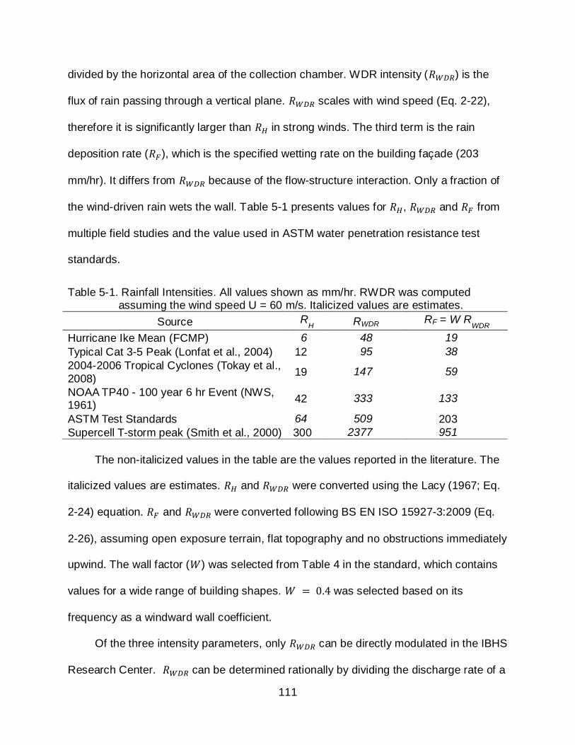
111
divided by the horizontal area of the collection chamber. WDR intensity ( ) is the
flux of rain passing through a vertical plane. scales with wind speed (Eq. 2-22),
therefore it is significantly larger than in strong winds. The third term is the rain
deposition rate ( ), which is the specified wetting rate on the building façade (203
mm/hr). It differs from because of the flow-structure interaction. Only a fraction of
the wind-driven rain wets the wall. Table 5-1 presents values for , and from
multiple field studies and the value used in ASTM water penetration resistance test
standards.
The non-italicized values in the table are the values reported in the literature. The
italicized values are estimates. and were converted using the Lacy (1967; Eq.
2-24) equation. and were converted following BS EN ISO 15927-3:2009 (Eq.
2-26), assuming open exposure terrain, flat topography and no obstructions immediately
upwind. The wall factor ( ) was selected from Table 4 in the standard, which contains
values for a wide range of building shapes. was selected based on its
frequency as a windward wall coefficient.
Of the three intensity parameters, only can be directly modulated in the IBHS
Research Center. can be determined rationally by dividing the discharge rate of a
Table 5-1. Rainfall Intensities. All values shown as mm/hr. RWDR was computed assuming the wind speed U = 60 m/s. Italicized values are estimates.
Source RH RWDR RF = W R
WDR
Hurricane Ike Mean (FCMP) 6 48 19 Typical Cat 3-5 Peak (Lonfat et al., 2004) 12 95 38 2004-2006 Tropical Cyclones (Tokay et al.,
2008)
19 147 59
NOAA TP40 - 100 year 6 hr Event (NWS, 1961) 42 333 133
ASTM Test Standards 64 509 203 Supercell T-storm peak (Smith et al., 2000) 300 2377 951

112
single nozzle (L3T-1) by the grid cell area (L2), which was nominally 660 mm x 610 mm.
Prior research (e.g. Choi, 1994; Blocken and Carmeliet, 2002) has shown that does
not vary significantly with wind speed. Therefore, the major challenge in this research
was to select a spray nozzle that would best replicate a naturally occurring RSD,
therefore resulting in a value approximately equal to 0.4. A nozzle with too many
small drops would cause a decrease in the parameter, and vice versa.
Spray Uniformity and the Effect of Wind Velocity on the Raindrop Size
Distribution
Manufacturer-supplied specifications for hydraulic spray nozzles typically include
the discharge rate, spray angle and spray pattern (circular or square). The RSD is not
given for off-the-shelf products, such as the nozzles considered in this study. Therefore
it was necessary to devise a test protocol to characterize the RSD of each nozzle.
Given the absence of information about the RSD, several questions needed to be
answered before this protocol could be developed:
1. Are the wetting rate and RSD uniform along the radial extent of the spray
pattern? Would one measurement suffice (and thereby save significant time and expense of testing) or are multiple measurements required to develop a composite RSD for the entire spray region?
2. How does the presence of wind change the RSD? Can the RSD characterization procedure be performed in still air, eliminating the need for expensive and time-
consuming tests?
To answer question 1, a simple experiment was performed to quantify the
variability of the spray using the apparatus shown in Figure 5-1a. A single nozzle was
aligned perpendicularly to the center of a vertically oriented collection chamber with 12
receivers. Each partition drained into its own graduated cylinder. The test consisted of
(1) covering the chamber, (2) setting the flow rate of the nozzle using a pressure
regulator, (3) removing the cover to allow water to enter the receivers, (4) covering the

113
chamber after five minutes, (5) shutting off the nozzle and (6) reading the graduated
cylinder and recording the accumulated water volume.
Ten nozzles were evaluated in this manner, and the results of all tests clearly
demonstrated a non-uniform wetting pattern. The most uniform spray pattern observed
in test series is shown in Figure 5-1B. The wetting rates varied by almost a factor of
three (123 – 301 mm/hr) with a coefficient of variation, CoV, of 0.25. The implication is
that multiple measurements inside the spray region would be required. This led to the
radial profiling technique discussed in the next section.
(a) Collection Chamber (b) Sample results for a BETE WL 1 1/2 nozzle
Figure 5-1. Apparatus to measure the spray uniformity of a single nozzle (photo
courtesy of author)
To answer question 2, a series of tests were performed in stagnant air and in a
steady jet generated by the wind generator at UF. The experimental configuration
consisted of an OTT PARSIVEL and DMT PIP located 3 m downwind of a 3 m x 3 m
uniform, open jet. The sensors were oriented horizontally such that the jet and laser
planes were parallel. Measurements were taken for wind velocity U = 8.9 m/s, 17.9 m/s,
and 35.8 m/s and compared to measurements taken in still air. The still air test was

114
performed with the nozzle facing downward and the PARSIVEL in an upright (standard)
position and located at the center of the circular spray area. Three tests were performed
for each case. The sampling duration was five minutes.
Results are shown in Figure 5-2. The vertical axis is the number concentration ,
which is the number of particles divided by a sample volume and diameter (dependent
on wind speed, Equation 2-28). The horizontal axis is the raindrop size diameter. The
wind speed and wind-driven rain intensity are shown in the legend. The figure
demonstrates that regardless of wind speed, the RSDs in the < 1 mm regime match the
stagnant air case for both instruments. Concentrations for drop diameters greater than 1
mm were greater than the stagnant air case; however, this behavior was expected and
attributed to the narrowing of the spray cone in the presence of wind. As the following
section will explain, all of the nozzles evaluated in stagnant air, ejected large droplets
( ) towards the outer edge of the spray area. Thus, as the spray cone
narrowed, a higher concentration of larger drops was expected.
The variation of the wind-driven rain intensities was attributed to the small sample
volumes resulting from five minute tests ). Mueller and Sims (1966)
determined that a minimum sample volume of is necessary to get reliable
estimates of the rainfall intensity and reflectivity (within 10% at a 95% confidence
interval). The required test time to achieve this sample volume (employing PARSIVEL
and PIP disdrometers) is a minimum of 15 minutes; however, this test duration was time
and cost prohibitive given the fuel, water, and labor resources necessary to operate the
wind generator.

115
The results from these tests indicate that the RSD behavior for the majority of the
drops (i.e., less than 1 mm) was unaffected by wind and the RSD of larger drops
behaved as expected. Therefore, an investigation of the characteristic nozzle RSD in
stagnant air was acceptable.
Figure 5-2. Comparison of raindrop size distributions measured in stagnant air and in a
steady wind by the PARSIVEL (left) and PIP (right, BETE WL 1 1/2 at 138 kPa)
Characterization of the Raindrop Size Distribution of a Spay Nozzles in Stagnant Air: A Proxy for Full-Scale Testing
Specimen Matrix
The 12 full cone hydraulic nozzles shown in Table 5-2 were selected for evaluation
based on their discharge rates and cost (> 450 nozzles are used in the IBHS Research
Center Full-Scale Test Facility).
Table 5-2. Spray nozzles evaluated in this study
BETE Lechler Steinen Spray Systems
WL 1 ½ 460.648.30.BE SM 151W 1/8GG-8W
WL 2 460.728.30.BE SM 303W 3/8GG-17W
WL 3 460.768.30.BE
TF 8 TF 10
0 1 2 3 410
-2
100
102
104
106
Diameter (mm)
Concentr
ation (
mm
-1 m
-3)
U = 0 m/s R
WDR = 509 mm/hr
U = 8.9 m/s, RWDR
= 172 mm/hr
U = 17.9 m/s, RWDR
= 155 mm/hr
U = 35.8 m/s, RWDR
= 36 mm/hr
0 1 2 3 410
-2
100
102
104
106
Diameter (mm)
Concentr
ation (
mm
-1 m
-3)
U = 0 m/s R
WDR = 509 mm/hr
U = 8.9 m/s, RWDR
= 977 mm/hr
U = 17.9 m/s, RWDR
= 1020 mm/hr
U = 35.8 m/s, RWDR
= 1050 mm/hr

116
Experimental Configuration
The experimental setup consisted of a 4.9 m x 4.9 m x 4.9 m chamber with
enclosed sides to reduce the effect of ambient wind. The nozzle was suspended 3.1 m
(10 m) above the ground in the center of the chamber facing downward. Four radial
extents were marked on the floor in 0.3 m increments, as shown in Figure 5-3. The
PARISIVELs were relocated to each position for five minutes of data capture.
Figure 5-3. PARSIVEL test locations for nozzle characterization
Analysis
The PARSIVEL outputs drop counts in a 32 x 32 matrix. Each cell corresponds to
a specific combination of drop diameter and fall velocity (see Chapter 2 for a detailed
explanation). Values were summed for all velocities for each diameter bin, and then
averaged over the four radial extents, yielding a 32 x 1 array of drop counts per
diameter along the radial extent. Results for one nozzle (BETE WL-3) are shown in
x x x x x x x xxxxxxxx
xxxxxxxx x x x x x x
3.05 m
Tests @ 0.31 m

117
Figure 5-4 for D = 0.31 mm to D = 3.8 m. The black lines correspond to the number of
drops as a function of radial distance from the centerline of the nozzle. The dashed lines
correspond to the maximum theoretical distance the particles should travel based on the
spray angle of the nozzle and the initial velocity. The governing equations for the
trajectory of a smooth rigid sphere acted upon by gravity and wind are Reynolds (Re)
number dependent. For Stokes flow conditions (Re < 1), the force acting on the raindrop
is equal to:
(5-1)
For 1<Re< 800, Schiller and Nauman (1933) define the drag coefficient and force as:
(5-2)
(5-3)
For 800<Re<105, Clift and Gauvin (1970) define the drag coefficient and force as:
(5-4)
(5-5)
where is the drag coefficient, is the force vector, is the Reynolds number,
is air density, is water density, is dynamic viscosity of air, is the drop
mass, is gravitational acceleration, is the cross-sectional area of each particle,
is the wind velocity vector, and is the velocity vector of the particles. The
acceleration ( ), velocity( ), and position ( ) are iteratively solved for each time
step as follows:

118
(5-6)
(5-7)
(5-8)
The initial velocities, i.e. , were determined using a Phantom V9.1 high
speed camera recording 1152 x 720 pixel images at 1000 fps and passed through an
edge filter (Figure 5-5).
It is evident from Figure 5-4 that the smaller particles tend to fall closer to the
centerline of the nozzle. The outermost fall locations match the theoretical estimates for
D = 0.68 mm to 1.68 mm. The particles that fell outside of this region exceeded the limit
due to the temporary walls not completely preventing air currents from forming inside of
the test chamber and water drops generating turbulence during their descent. For the
smaller drops, wind velocities as low as 0.1 m/s are sufficient to cause the deviation
observed in the data. The larger drops did not reach the theoretical limit and tended to
fall further from the center of the spray area. This behavior was observed visually in all
of the nozzles and is hypothesized to be a result of the higher momentum of the larger
drops. The helical ducting in the nozzles (all of the nozzles had similar designs)
introduces an angular velocity component into the flow; consequently, larger drops
(higher mass) have a higher tangential momentum and are ejected farther from the
center. Plots of the other nozzles (see appendix) demonstrate that the spray pattern for
all nozzles was similar.

119
Figure 5-4. Count of drops radially outward from nozzle centerline
0 1 2 3 40
1
2
3x 10
4
r (m)
# D
rop
s
D = 0.31 mm
0 1 2 3 40
2
4
6x 10
4
r (m)
# D
rop
s
D = 0.44 mm
0 1 2 3 40
2
4
6x 10
4
r (m)
# D
rop
s
D = 0.56 mm
0 1 2 3 40
2
4x 10
4
r (m)
# D
rop
s
D = 0.69 mm
0 1 2 3 40
1
2x 10
4
r (m)
# D
rop
s
D = 0.81 mm
0 1 2 3 40
5000
10000
r (m)
# D
rop
s
D = 0.94 mm
0 1 2 3 40
5000
r (m)
# D
rop
s
D = 1.1 mm
0 1 2 3 40
2000
4000
r (m)
# D
rop
s
D = 1.2 mm
0 1 2 3 40
2000
4000
r (m)
# D
rop
s
D = 1.4 mm
0 1 2 3 40
1000
2000
r (m)
# D
rop
s
D = 1.6 mm
0 1 2 3 40
500
1000
1500
r (m)
# D
rop
s
D = 1.9 mm
0 1 2 3 40
500
1000
r (m)
# D
rop
s
D = 2.1 mm
0 1 2 3 40
200
400
r (m)
# D
rop
s
D = 2.4 mm
0 1 2 3 40
200
400
600
r (m)
# D
rop
s
D = 2.8 mm
0 1 2 3 40
50
100
150
r (m)
# D
rop
sD = 3.3 mm
0 1 2 3 40
10
20
30
r (m)
# D
rop
s
D = 3.8 mm

120
Figure 5-5. Determining initial velocity using high speed footage (photo courtesy of
author)
To compute the number of drops per diameter for the entire spray region from the
data averaged over the radial extent, each array was integrated using the method of
circular discs:
(5-9)
where is the total number of drops of diameter , is the radial distance from
the center to the measurement location, is the number of observed diameter
droplets at location and is the sample area of the PARSIVEL.
The nozzle flow rate was also computed from the PARISVEL data to verify mass
continuity:
(5-10)
where is the flow rate, and is the sample time. The estimated values agreed very
well with the known discharge values. Errors were on the order of 15% or less.
The RSD of each nozzle was calculated from:

121
(5-11)
where is the circular spray area and is the terminal velocity of a diameter drop.
Figure 5-6 shows the calculated RSD for all of the nozzles (RSDs of other nozzles are
independently listed in the appendix). As the figure shows, the major difference in the
RSD of the nozzles was the number concentration of large particles. The concentration
of smaller particles was virtually identical for raindrop diameters <= 1.0 mm. Therefore
the selection of the BETE WL3 was made based on achieving the largest number of
large drops in the flow.
Figure 5-6. Raindrop size distribution of BETE WL3 in stagnant air conditions
0 1 2 3 4 510
-4
10-2
100
102
104
106
Diameter (mm)
Co
nce
ntr
atio
n, N
D (
mm
-1 m
-3)
BETE WL3
Other Nozzles
Best (1950)

122
Validation of the Wind-Driven Rain Simulation System at the IBHS Research Facility
Upon selection of the nozzle, the wind-driven rain simulation system was
constructed. The system consists of three nozzle grids for each of the three horizontal
fan cells. The flow rate and pressure of each grid is actively controlled by automated
gate valves. Horizontal nozzle spacing was limited to either 1320 mm or 66 mm due to
the 1320 mm spacing of the air foils. It was observed from testing at UF that the shorter
horizontal spacing would yield a more uniform spray, particularly in high wind speeds;
thus, 660 mm was selected. Similarly, shorter vertical spacing would yield more uniform
spray patterns; however, the closer the spacing, the lower the required pressure and
flow rate per nozzle. The lowest pressure recommended by the manufacturers was
34.5 kPa; thus, the minimum vertical spacing required was 610 mm.
To validate the design recommendations, a PARSIVEL and PIP were used to take
RSD measurements at multiple locations in the stream. The instruments were placed
on vertical steel lattices at 10 m and 3 m from the air foils (Figure 5-7). Flow rates were
determined to be approximately 3.8 L/min per nozzle (using inline digital flow gauges,
corresponds to approximately 34.5 kPa). Five minute measurements of the RSD were
taken at 2.0 m, 3.0 m, 4.0 m, 5.2 m, and 6.0 m for each wind speed. The measured
RSDs matched the RSD predicted by the Best (1950) model at an intensity of 509
mm/hr, confirming the choice of nozzle and spacing (Figure 5-8). The mean of all the
RSDs also agreed with the Best (1950) model (Figure 5-9). This observation implies
that for full scale simulations, the wetting rate reaching the building façade will be
approximately 203 mm/hr and the RSD will be representative of natural conditions.

123
Figure 5-7. Instrument arrangement at the Insurance Institute for Business & Home Safety Research Center (photo courtesy of author)

124
Figure 5-8. Measured raindrop size distributions at multiple heights and wind velocities
0 1 2 3 4 5
101
104
107
U = 8.9 m/sZ
= 1
.8 m
0 1 2 3 4 5
101
104
107
U = 17.9 m/s
0 1 2 3 4 5
101
104
107
U = 26.8 m/s
0 1 2 3 4 5
101
104
107
Z =
2.7
m
0 1 2 3 4 5
101
104
107
0 1 2 3 4 5
101
104
107
0 1 2 3 4 5
101
104
107
Z =
3.7
m
0 1 2 3 4 5
101
104
107
0 1 2 3 4 5
101
104
107
0 1 2 3 4 5
101
104
107
Z =
5.2
m
0 1 2 3 4 5
101
104
107
0 1 2 3 4 5
101
104
107
0 1 2 3 4 5
101
104
107
Z =
6.0
m
Diameter (mm)0 1 2 3 4 5
101
104
107
Diameter (mm)0 1 2 3 4 5
101
104
107
Diameter (mm)
Parsivel Measurement PIP MeasurementBest (1950) ModelBased on 509 mm/hr

125
Figure 5-9. Comparison of measured raindrop size distributions and Best (1950) model
Summary
This chapter presented the design of a realistic wind-driven rain simulation system
that can reproduce the rainfall intensity and drop size distributions obtained from the
field measurement activities (Chapter 4). The simulation system was implemented at
the Insurance Institute for Business & Home Safety Research Facility for the water
penetration resistance evaluation of low-rise buildings. The following chapter will
summarize contributions and conclusions of the research described in this document
and present recommendations for future studies.
0 1 2 3 4 510
0
101
102
103
104
105
106
Co
nce
ntr
atio
n (
mm
-1 m
-3)
Diameter (mm)
Parsivel Mean
PIP Mean
Best (1950) Model for R = 509 mm/hr

126
CHAPTER 6
SUMMARY, CONCLUSIONS,AND RECOMMENDATIONS
This chapter summarizes the efforts taken to advance the knowledge base by
characterizing extreme wind-driven rain (WDR) events, creating and evaluating a WDR
measurement technique, and the design of a full scale WDR simulation system.
Characterization of Extreme Wind-Driven Rain Events
The VORTEX2 and FCMP field campaigns yielded 17 thunderstorm and two
tropical cyclone datasets. For these activities, a novel approach was taken to minimize
errors associated with strong winds. The instrumentation platforms continuously align
the disdrometers towards the mean rain vector using continuous wind velocity and
direction feedback. The first instrument platform was designed to be mounted on one of
the ruggedized FCMP meteorological measurement stations to record rain data at 3m
and wind data at 5m; however, the employed disdrometer was cost prohibitive when
considering a multiple instrument array. Thus, as part of this project, a low cost, easy to
handle, robust instrument platform was designed and constructed.To achieve a low cost
solution (20% of the cost of the high performance disdrometer) OTT PARSIVELs were
employed; however, the OTT PARSIVELs have a lower resolution and sampling rate
than the DMT PIP. Moreover, the disdrometer is not intended to be used in strong
winds. Thus, three laboratory experiments were conducted to investigate the errors
exhibited by the PARSIVEL associated with strong winds.
Proof of Concept
The first two experiments were measurements of the raindrop size distribution
(RSD) emitted from a nozzle in stagnant air conditions. One test compared the
measured RSD of the PARSIVEL to the RSD determined by a morphological image

127
processing algorithm that was created to count the number of droplets captured in an oil
medium. Results demonstrated that for practical purposes, when the PARSIVEL is
oriented towards the mean rain direction, the measured RSDs compared favorably to
those measured by the image processing algorithm.
The second test evaluated the effect of oblique trajectory angles on the measured
diameter and velocities. High tolerance steel bearings, of multiple diameters, were
dropped through the laser band of the PARSIVEL and different angles. The different
angles replicated the effect of wind on droplets passing through the measurement area
of a stationary instrument (i.e. laser band continuously parallel to the ground). These
tests revealed that at oblique trajectory angles, diameters of drops are measured with
high fidelity; however, the measured velocities are unrealistically reduced. The
consequence is unrealistic large number concentrations ( ).
The third laboratory experiment compared measurements from the PARSIVEL,
oriented at different angles, and a DMT PIP mounted on a gantry system exposed to
multiple wind speeds and rainfall intensities. Results from these tests confirmed the
findings from the stagnant air tests; the PARSIVELs exhibited erroneous measurements
resulting from incorrect orientation which are magnified by higher wind velocities.
These observations validated the concept taken in the design of the articulating
instrumentation platforms. The articulating instrumentation platforms continuously
aligned the disdrometers such that the laser plane was perpendicular to the mean rain
vector. Field data from collocated stationary and articulating instrumentation platforms
confirm that in moderately high wind speeds (> 10 m/s), data from the stationary

128
instrumentation becomes compromised; while the data from the articulating
instrumentation exhibited no wind induced error.
Conclusions from Field Data Results
The simultaneous wind and rain data gathered by the articulating instruments, to
the author’s knowledge, has been the first attempt at characterizing ground level free-
stream RSDs in extreme wind events. Thus, as part of the research project the following
five topics were investigated:1) the effect of wind on the drop diameter, 2) the effect of
wind on the RSD, 3) comparison of RSD Models to RSDs measured in multiple wind
velocities, 4) calculation of the peak to mean ratios of , and 5) comparison of rain data
measured in extreme events to WSR-88D data.
Effect of wind velocity and turbulence intensity on raindrop diameter
The effect of wind velocity and turbulence intensity on raindrop size was
investigated using data from both field campaigns. Two main trends were observed: 1)
mean drop diameter tends to increase with increased wind velocity and 2) mean drop
diameter tends to decrease in the presence of high turbulence intensities. The cause of
these trends is postulated to be attributable to one or both of the following possibilities:
1) It is possible that in increased wind velocities the high drag forces acting on the
droplets overcome the surface tension holding the shape together and breakup occurs
or 2) high turbulence intensities cause the probability of coalescence to increase.
These conclusions are intended to motivate further study. This is a limited dataset and
more data is necessary for a comprehensive study to be performed and definite
conclusions to be made.

129
wind velocity and turbulence intensity dependency of the raindrop size distribution
Observations of drop diameter changing in the presence of multiple wind
scenarios led to investigate the effect of wind on the RSD. For this investigation, wind
velocity, turbulence intensities, and the gamma parameters for each one minute
segment of VORTEX2 and FCMP data were calculated. These data (Figure 4-11)
suggest that , , and remain constant with increasing longitudinal velocity, and
longitudinal and lateral turbulence intensities; however, the variance of each of the
variables decreased with increasing longitudinal velocity. Thus, it was concluded that
that the RSD does not significantly change with increased wind speed, or longitudinal
and lateral turbulence intensities.
When investigating the relationship between and , (Figure 5-12) it was
observed that the measured relationship differs from the empirical relationship
established by Zhang (2003, Equation 5-12). A possible source for the difference is that
there are too few one minute measurements. If the observed relationship is valid, the
implication could ultimately mean incorrect interpretation of RSD parameters from
reflectivity measurements. Presently, the reason for the dissimilarity is unclear and
more data is necessary to make an assessment.
Comparison of Measured Data to Raindrop Size Distribution Models
RSD models are used by the wind engineering community as a simple technique
to acquire an adequate RSD for WDR modeling. Thus, an evaluation of the applicability
of current RSD models to data gathered in strong winds was performed. Field
measured data was compared to the Marshall and Palmer (1948), Best (1950), and
Willis and Tattleman (1989) dependent models and the gamma model using the mean

130
parameters from the measured data. The results indicate that the difference in the
performance of the models below or above 15 m/s, below or above 0.2 , or below or
above 0.2 (Figures 5-18 – 5-20) was insignificant. The data also shows that the Best
(1950) model yields the least error and is thus the most accurate.
Comparison of Measured Data to WSR-88D Data
FCMP Hurricane Ike data were compared with remotely sensed estimates from
the National Weather Service WSR-88D Doppler Radar KHGX. Generally, there was
good agreement between disdrometer estimated and radar measured reflectivities. The
data shows that there is also relatively good agreement between the ground level
measured rainfall intensity and the radar estimated rainfall intensity below 10 mm/hr.
Above 10 mm/hr the default Z-R relationship, employed at KHGX, underestimated the
observed rainfall intensity. Thus, other commonly used empirical Z-R relationships
(Table 5.3, as recommended by the WSR-88D Operational Support Facility) were
compared. Of the recommended relationships, the Rosenfeld tropical relationship more
closely resembled the observed data; however, all of the Z-R relationships
underestimated the observed rainfall.
Peak to Mean Ratio of Rainfall Intensities
Peak to mean ratios of rainfall intensities were calculated for their potential use in
design practice. Currently, the widely accepted standard (BSI EN ISO 15927-3)
calculates the rain deposition rate from hourly and data. The research
demonstrates that designing for a shorter duration peak can significantly increase the
design wind driven rainfall intensity ( ) and subsequently, the deposition rate ( ).
For instance, using 10 minute FCMP Hurricane Ike data, the design free-stream wind
driven rain intensity is approximately three times larger than using hourly data. For

131
design, the applicability of a peak to mean ratio would depend on site specific
probabilities of type of precipitation and wind speed. The presented research shows the
potential value of peak to mean ratios of rainfall intensities in design practice; however,
more data should be collected to assess the validity of the peak to mean ratio curves
presented herein.
Design and Implementation of a Full Scale Wind-Driven Rain System
The Insurance Institute for Business & Home Safety tasked researchers at the
University of Florida with the design of a WDR simulation system for the IBHS Research
Center Full Scale Test Facility. The design was based on field measured RSD data and
intended to reproduce the rain deposition rate specified in current test standards. The
methodology consisted of characterizing the nozzles’ and RSD, selecting the most
appropriate nozzle, and validating the full-scale WDR simulation system.
Nozzle Characterization
The OTT PARSIVEL was utilized to investigate the characteristics of nozzles
whose manufacturers’ specifications indicate the approximate necessary flow rate.
Measurements in the presence of wind revealed that there was negligible change in the
RSD indicating that the particles accelerated with the flow with little interaction. Thus, it
was deemed acceptable to characterize the RSD of individual nozzles in stagnant air.
Of the tested nozzles, the BETE WL-3 exhibited an RSD that closely resembled the
Best (1950) RSD model (the model that best fit field measured data). Nozzle spacing
was set to the minimum possible spacing given space and flow rate limitations.
Full Scale Implementation
Upon determining the spray system characteristics, the rain simulation system was
constructed at the IBHS Research Center. Free-stream WDR measurements were

132
taken at the facility with the PARSIVEL and the PIP at multiple locations in the stream.
The measurements indicate that the RSD closely resembles the RSD predicted by the
Best (1950) model. Thus, future full scale simulations will be representative of natural
conditions.
Recommendations for Future Research
Recommendations for Instrumentation
Construction of more instrument platforms will facilitate the investigation of the
spatial correlation of WDR. The instruments can also be easily adapted to make tower
mounted meteorological observations. Thus, the vertical and horizontal evolution of
WDR can be investigated.
Currently the design of the articulating instrumentation platforms allows for the
upgrade of real-time data streaming. The availability of real-time data streaming may
aid agencies such as meteorological institutions in updating forecasts, emergency
management agencies in assignment of resources during and after extreme events, and
FCMP teams responding to errors by instrumentation during data acquisition.
Future research, utilizing the articulating instrument platforms would benefit from
the implementation of GPS and compass instrumentation. These digital measurements
would enable real time processing of cardinal wind direction and global position.
Currently, the algorithm that aligns the disdrometers to the mean rain vector
assumes a mean drop diameter of 1.2 mm, a valid assumption for extreme rainfall
scenarios. A new tracking algorithm that aligns the disdrometer to the measured mean
drop size may expand the use of the instrumentation platforms to other applications and
decrease the occurrence of, otherwise unknown, incorrectly measured data.

133
PARSIVEL validation results from this research project indicate that the error
introduced by oblique trajectory angles manifest as incorrect velocities, while droplet
diameters are measured correctly. A new data processing algorithm may be created to
utilize real time wind data for the calculation of droplet velocities rather than residence
time in the measurement field. This new measurement technique may provide a way of
increasing the maximum acceptable wind speed when using stationary instrumentation.
Recommendations for Full Scale and Numerical Models
The implementation of a full scale WDR simulation system that accurately
simulates naturally occurring RSDs may be used in the validation of numerical WDR
models by implementing similar structures in the models and the IBHS Research
Facility. The full scale simulation system will also prove useful in the evaluation of
building component performance.
The data gathered from field measurements can be used in time varying full-scale
simulations of extreme WDR scenarios. Thus, future experiments could compare the
performance of building components subjected to current testing protocols and
simulations based on field measured data to establish the efficacy current standardized
test methods.
Current numerical WDR models make a Stoke’s flow assumption (Re << 1) to
determine the driving forces of particles moving through space. Implementing a wind
field determined by a CFD software package to the developed trajectory model will
result in a new Reynold’s number dependent WDR model. Such a model may yield
better results and warrants further research.

134
Recommendations for the Morphological Image Processing Algorithm
The design of a robust graphical user interface for the morphological image
processing algorithm would serve as an economical solution to RSD measurement.
When compared to disdrometric instrumentation, it is a labor intensive process;
however, it may be a useful tool for applications where the drop size distribution is
known to remain constant or for instrumentation validation.
If the morphologic image processing algorithm and Reynold’s number dependent
trajectory model are made available to the public, they may be used by nozzle
manufacturers and designers for the characterization of nozzles and for the design of
custom water delivery applications. To the author’s knowledge, no such design tool is
currently available.

135
APPENDIX
Theoretical Proof of Greater Accuracy from an Articulating Instrument
This proof follows the work of Griffiths (1974) in which he demonstrated that the
sample volume for an articulating instrument is different than that of a stationary
instrument. Ultimately, it is shown that the articulating sensor has a greater accuracy
due to the greater sample volume.
Case 1 represents a stationary instrument oriented such that the sample area is
oriented parallel to the ground, Case 2 and 3 represent an articulating instrument
platform such that the sample area is tilted to angle (determined by the trajectory of
the assumed mean droplet diameter) and other droplets are crossing the sample area at
angle depending whether the droplet is smaller than assumed mean (Case 2) or
larger (Case 3).
S = Sample area (m2) VTD = Terminal velocity of droplets of diameter D (m/s)
U = Longitudinal wind velocity (m/s)
VRD = Resultant velocity of droplets of diameter D (m/s)
CD = Number density of droplets of diameter D (m-1)
nDΦ = Number of droplets of diameter D having trajectory Φ collected per sec (sec-1)
VS = Sample volume (m3)
MDΦ = Total number of droplets having trajectory Φ collected over time T
ND = Number concentration of droplets of diameter D
Case 3 Case 2 Case 1

136
Stationary instrument (Case 1):
If we collect data for Time T and say total number of droplets = MDΦ:
We know:
Thus:
Solve for concentration of droplets:
Given:
Thus we find that the sample volume for a stationary instrument is:

137
Articulating instrumentation (Case 2 & 3)
Using the following identities:
We get the following for both Case 2 and 3:
We know:
Substitution gives us:
Check for Φ = 90 (Case where U = 0):
Checks
Say :
If we collect data for Time T and say total number of droplets = MD,Φ:
Solve for concentration of droplets:
Thus we find that the sample volume for an articulating instrument is:

138
Compare Instrumentation platforms:
Given we know:
for stationary instrumentation
for articulating instrumentation
K can vary from U to VT,D . If the tracking algorithm is accurate, in high winds K
approaches U and VT,D in no wind
for stationary instrumentation
for articulating instrumentation in no wind
for articulating instrumentation in high winds
Therefore as the wind speed increases the sample volume of the articulating instrument
platform increases, making it more accurate. Example: Assuming that the mean drop diameter is 1.2 mm and U = 10 m/s:
Ф as the tracking algorithm calculates it
for stationary instrumentation
for articulating instrumentation
Thus the sample volume of articulating instrument is greater than twice as large at U =
10 m/s. Similarly the ratio of the sample volumes can be calculated for multiple wind velocities:
U V T , (1.2 m m ) φ K V S ratio
0 4.64 1.57 4.64 1.00
5 4.64 0.75 6.82 1.47
10 4.64 0.43 11.02 2.38
15 4.64 0.30 15.70 3.38
20 4.64 0.23 20.53 4.42
25 4.64 0.18 25.43 5.48
30 4.64 0.15 30.36 6.54

139
Nozzle Selection
Nozzles are used in a wide range of applications, including evaporative cooling,
gas conditioning, fire suppression, spray drying, and agriculture. Nozzles generate
droplets through the process of atomization, in which a fluid with a potential energy
(water pressure) is released through an opening (nozzle end) and emerge as ligaments
that evolve into droplets (Schick 1997). The resultant drop size distribution is a function
of the nozzle type, spray type, spray angle, and the pressure and flow rate of the fluid.
Figure A-1. Droplet formation process

140
Figure A-2. Types of nozzles and drop size relationship
The effect of each variable is as follows:
Nozzle types, which can be hydraulic or air assisted. Air assisted nozzles
generally produce droplets in a smaller size range than hydraulic nozzles.
Spray types are flat, solid stream, square, hollow cone, and full cone
sprays. Full cone and square spray nozzles produce the largest drop size
distribution followed by flat spray and hollow cone spray nozzles (Fig 4-2).
Spray angle—the angle through which the spray is effective—is inversely
proportional to drop size.
Nozzle pressure is inversely proportional to drop size and is controlled by
the pumping system.
Flow rate is directly proportional to the drop size and controlled by an
actively controlled valve system.

141
Measured Diameter – Wind Relationships
Hurricane Ike Data

142

143

144
Hurricane Irene (Beaumont) Data

145

146

147
Hurricane Irene (Deal) Data

148

149

150
Florida Coastal Monitoring Program Hurricane Ike Data

151

152

153
Verification of the Origins of Rotation in Tornadoes Experiment 2 Articulating Instrument Platform Data
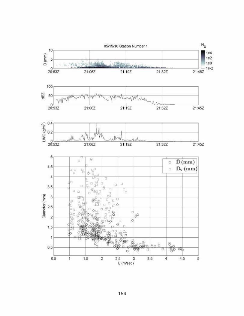
154

155

156
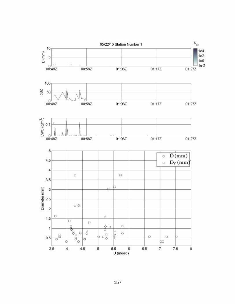
157

158

159

160

161

162

163

164

165

166

167

168

169

170
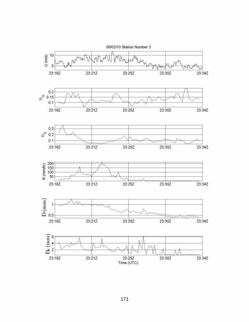
171

172

173

174

175

176

177

178

179

180

181

182

183

184

185

186

187

188

189

190

191
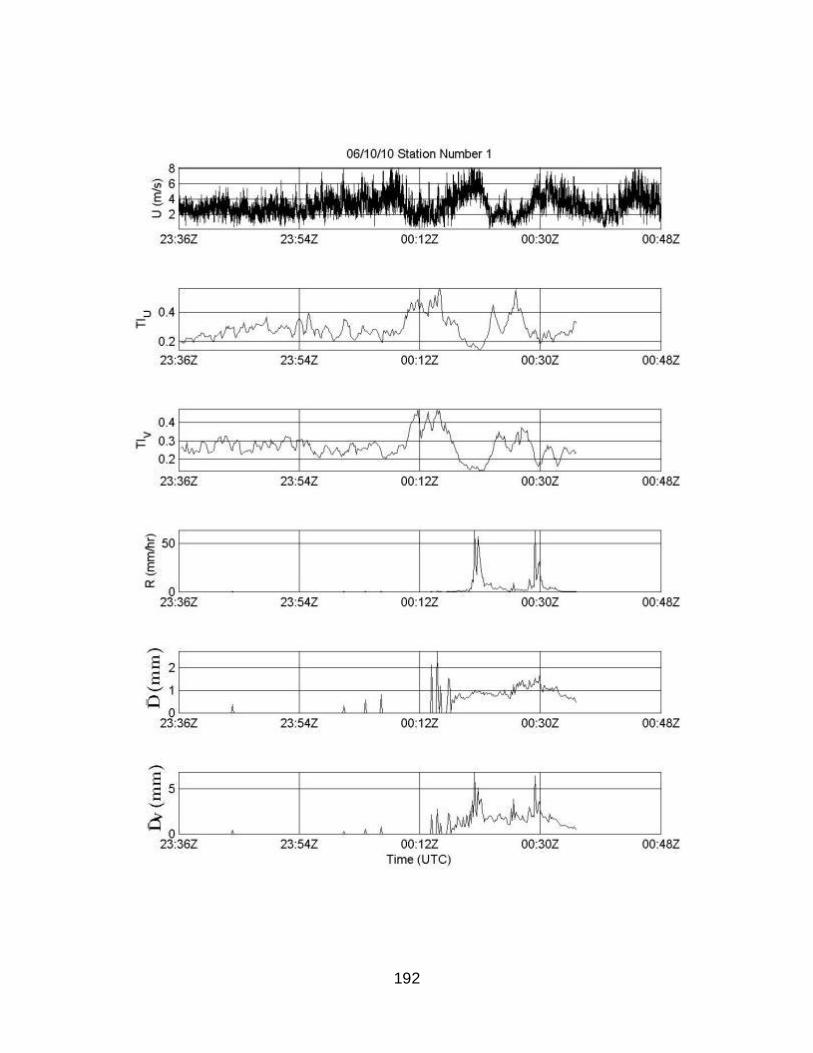
192

193

194

195

196

197

198

199

200

201

202

203

204

205

206

207

208

209

210
Measured Nozzle Characteristics
Uniformity
BETE WL-1
0 1 2 3 40
2
4x 10
4
r (m)
# D
rop
s
D = 0.31 mm
0 1 2 3 40
5
10x 10
4
r (m)
# D
rop
s
D = 0.44 mm
0 1 2 3 40
5
10x 10
4
r (m)
# D
rop
s
D = 0.56 mm
0 1 2 3 40
2
4x 10
4
r (m)
# D
rop
s
D = 0.69 mm
0 1 2 3 40
1
2x 10
4
r (m)
# D
rop
s
D = 0.81 mm
0 1 2 3 40
5000
10000
r (m)
# D
rop
s
D = 0.94 mm
0 1 2 3 40
1000
2000
r (m)
# D
rop
s
D = 1.1 mm
0 1 2 3 40
200
400
r (m)
# D
rop
s
D = 1.2 mm
0 1 2 3 40
200
400
r (m)
# D
rop
s
D = 1.4 mm
0 1 2 3 40
100
200
r (m)
# D
rop
s
D = 1.6 mm
0 1 2 3 40
20
40
r (m)
# D
rop
s
D = 1.9 mm
0 1 2 3 40
5
10
r (m)
# D
rop
s
D = 2.1 mm
0 1 2 3 40
0.5
1
r (m)
# D
rop
s
D = 2.4 mm
0 1 2 3 4-1
0
1
r (m)
# D
rop
s
D = 2.8 mm
0 1 2 3 4-1
0
1
r (m)
# D
rop
s
D = 3.3 mm
0 1 2 3 4-1
0
1
r (m)
# D
rop
s
D = 3.8 mm

211
BETE WL-2
0 1 2 3 40
2
4x 10
4
r (m)
# D
rop
s
D = 0.31 mm
0 1 2 3 40
5
10x 10
4
r (m)
# D
rop
s
D = 0.44 mm
0 1 2 3 40
5
10x 10
4
r (m)
# D
rop
s
D = 0.56 mm
0 1 2 3 40
2
4x 10
4
r (m)
# D
rop
s
D = 0.69 mm
0 1 2 3 40
1
2x 10
4
r (m)
# D
rop
s
D = 0.81 mm
0 1 2 3 40
5000
10000
r (m)
# D
rop
sD = 0.94 mm
0 1 2 3 40
2000
4000
r (m)
# D
rop
s
D = 1.1 mm
0 1 2 3 40
2000
4000
r (m)
# D
rop
s
D = 1.2 mm
0 1 2 3 40
2000
4000
r (m)
# D
rop
s
D = 1.4 mm
0 1 2 3 40
1000
2000
r (m)
# D
rop
s
D = 1.6 mm
0 1 2 3 40
500
1000
r (m)#
Dro
ps
D = 1.9 mm
0 1 2 3 40
500
r (m)
# D
rop
s
D = 2.1 mm
0 1 2 3 40
200
400
r (m)
# D
rop
s
D = 2.4 mm
0 1 2 3 40
200
400
r (m)
# D
rop
s
D = 2.8 mm
0 1 2 3 40
50
100
r (m)
# D
rop
s
D = 3.3 mm
0 1 2 3 40
5
10
r (m)
# D
rop
s
D = 3.8 mm

212
BETE WL-1 1/2
0 1 2 3 40
2
4x 10
4
r (m)
# D
rop
s
D = 0.31 mm
0 1 2 3 40
5
10x 10
4
r (m)
# D
rop
s
D = 0.44 mm
0 1 2 3 40
5
10x 10
4
r (m)
# D
rop
s
D = 0.56 mm
0 1 2 3 40
5x 10
4
r (m)
# D
rop
s
D = 0.69 mm
0 1 2 3 40
2
4x 10
4
r (m)
# D
rop
s
D = 0.81 mm
0 1 2 3 40
5000
10000
r (m)
# D
rop
sD = 0.94 mm
0 1 2 3 40
2000
4000
r (m)
# D
rop
s
D = 1.1 mm
0 1 2 3 40
1000
2000
r (m)
# D
rop
s
D = 1.2 mm
0 1 2 3 40
1000
2000
r (m)
# D
rop
s
D = 1.4 mm
0 1 2 3 40
500
1000
r (m)
# D
rop
s
D = 1.6 mm
0 1 2 3 40
200
400
r (m)#
Dro
ps
D = 1.9 mm
0 1 2 3 40
100
200
r (m)
# D
rop
s
D = 2.1 mm
0 1 2 3 40
100
200
r (m)
# D
rop
s
D = 2.4 mm
0 1 2 3 40
20
40
r (m)
# D
rop
s
D = 2.8 mm
0 1 2 3 40
5
10
r (m)
# D
rop
s
D = 3.3 mm
0 1 2 3 40
0.5
1
r (m)
# D
rop
s
D = 3.8 mm

213
BETE WL-3
0 1 2 3 40
2
4x 10
4
r (m)
# D
rop
s
D = 0.31 mm
0 1 2 3 40
5
10x 10
4
r (m)
# D
rop
s
D = 0.44 mm
0 1 2 3 40
5
10x 10
4
r (m)
# D
rop
s
D = 0.56 mm
0 1 2 3 40
2
4x 10
4
r (m)
# D
rop
s
D = 0.69 mm
0 1 2 3 40
1
2x 10
4
r (m)
# D
rop
s
D = 0.81 mm
0 1 2 3 40
5000
10000
r (m)
# D
rop
s
D = 0.94 mm
0 1 2 3 40
5000
r (m)
# D
rop
s
D = 1.1 mm
0 1 2 3 40
2000
4000
r (m)
# D
rop
s
D = 1.2 mm
0 1 2 3 40
2000
4000
r (m)
# D
rop
s
D = 1.4 mm
0 1 2 3 40
1000
2000
r (m)
# D
rop
s
D = 1.6 mm
0 1 2 3 40
1000
2000
r (m)#
Dro
ps
D = 1.9 mm
0 1 2 3 40
500
1000
r (m)
# D
rop
s
D = 2.1 mm
0 1 2 3 40
200
400
r (m)
# D
rop
s
D = 2.4 mm
0 1 2 3 40
500
r (m)
# D
rop
s
D = 2.8 mm
0 1 2 3 40
100
200
r (m)
# D
rop
sD = 3.3 mm
0 1 2 3 40
20
40
r (m)
# D
rop
s
D = 3.8 mm

214
Lechler 608
0 1 2 3 40
2
4x 10
4
r (m)
# D
rop
s
D = 0.31 mm
0 1 2 3 40
5x 10
4
r (m)
# D
rop
s
D = 0.44 mm
0 1 2 3 40
5x 10
4
r (m)
# D
rop
s
D = 0.56 mm
0 1 2 3 40
2
4x 10
4
r (m)
# D
rop
s
D = 0.69 mm
0 1 2 3 40
1
2x 10
4
r (m)
# D
rop
s
D = 0.81 mm
0 1 2 3 40
5000
10000
r (m)
# D
rop
s
D = 0.94 mm
0 1 2 3 40
2000
4000
r (m)
# D
rop
s
D = 1.1 mm
0 1 2 3 40
1000
2000
r (m)
# D
rop
s
D = 1.2 mm
0 1 2 3 40
500
1000
r (m)
# D
rop
s
D = 1.4 mm
0 1 2 3 40
500
r (m)
# D
rop
s
D = 1.6 mm
0 1 2 3 40
100
200
r (m)#
Dro
ps
D = 1.9 mm
0 1 2 3 40
20
40
r (m)
# D
rop
s
D = 2.1 mm
0 1 2 3 40
10
20
r (m)
# D
rop
s
D = 2.4 mm
0 1 2 3 40
5
10
r (m)
# D
rop
s
D = 2.8 mm
0 1 2 3 40
0.5
1
r (m)
# D
rop
sD = 3.3 mm
0 1 2 3 4-1
0
1
r (m)
# D
rop
s
D = 3.8 mm

215
Lechler 648
0 1 2 3 40
2
4x 10
4
r (m)
# D
rop
s
D = 0.31 mm
0 1 2 3 40
5
10x 10
4
r (m)
# D
rop
s
D = 0.44 mm
0 1 2 3 40
5
10x 10
4
r (m)
# D
rop
s
D = 0.56 mm
0 1 2 3 40
5x 10
4
r (m)
# D
rop
s
D = 0.69 mm
0 1 2 3 40
2
4x 10
4
r (m)
# D
rop
s
D = 0.81 mm
0 1 2 3 40
1
2x 10
4
r (m)
# D
rop
s
D = 0.94 mm
0 1 2 3 40
5000
r (m)
# D
rop
s
D = 1.1 mm
0 1 2 3 40
1000
2000
r (m)
# D
rop
s
D = 1.2 mm
0 1 2 3 40
1000
2000
r (m)
# D
rop
s
D = 1.4 mm
0 1 2 3 40
500
1000
r (m)
# D
rop
s
D = 1.6 mm
0 1 2 3 40
200
400
r (m)#
Dro
ps
D = 1.9 mm
0 1 2 3 40
100
200
r (m)
# D
rop
s
D = 2.1 mm
0 1 2 3 40
50
100
r (m)
# D
rop
s
D = 2.4 mm
0 1 2 3 40
50
r (m)
# D
rop
s
D = 2.8 mm
0 1 2 3 40
10
20
r (m)
# D
rop
sD = 3.3 mm
0 1 2 3 40
2
4
r (m)
# D
rop
s
D = 3.8 mm

216
Spray Systems 1/8GG
0 1 2 3 40
2
4x 10
4
r (m)
# D
rop
s
D = 0.31 mm
0 1 2 3 40
5
10x 10
4
r (m)
# D
rop
s
D = 0.44 mm
0 1 2 3 40
5x 10
4
r (m)
# D
rop
s
D = 0.56 mm
0 1 2 3 40
2
4x 10
4
r (m)
# D
rop
s
D = 0.69 mm
0 1 2 3 40
1
2x 10
4
r (m)
# D
rop
s
D = 0.81 mm
0 1 2 3 40
5000
10000
r (m)
# D
rop
s
D = 0.94 mm
0 1 2 3 40
2000
4000
r (m)
# D
rop
s
D = 1.1 mm
0 1 2 3 40
2000
4000
r (m)
# D
rop
s
D = 1.2 mm
0 1 2 3 40
2000
4000
r (m)
# D
rop
s
D = 1.4 mm
0 1 2 3 40
500
1000
r (m)
# D
rop
s
D = 1.6 mm
0 1 2 3 40
200
400
r (m)#
Dro
ps
D = 1.9 mm
0 1 2 3 40
100
200
r (m)
# D
rop
s
D = 2.1 mm
0 1 2 3 40
20
40
r (m)
# D
rop
s
D = 2.4 mm
0 1 2 3 40
10
20
r (m)
# D
rop
s
D = 2.8 mm
0 1 2 3 40
1
2
r (m)
# D
rop
sD = 3.3 mm
0 1 2 3 4-1
0
1
r (m)
# D
rop
s
D = 3.8 mm

217
Steinen 100
0 1 2 3 40
2
4x 10
4
r (m)
# D
rop
sD = 0.31 mm
0 1 2 3 40
5
10x 10
4
r (m)
# D
rop
s
D = 0.44 mm
0 1 2 3 40
5
10x 10
4
r (m)
# D
rop
s
D = 0.56 mm
0 1 2 3 40
5x 10
4
r (m)
# D
rop
s
D = 0.69 mm
0 1 2 3 40
2
4x 10
4
r (m)
# D
rop
s
D = 0.81 mm
0 1 2 3 40
5000
10000
r (m)
# D
rop
s
D = 0.94 mm
0 1 2 3 40
2000
4000
r (m)
# D
rop
s
D = 1.1 mm
0 1 2 3 40
1000
2000
r (m)
# D
rop
s
D = 1.2 mm
0 1 2 3 40
1000
2000
r (m)
# D
rop
s
D = 1.4 mm
0 1 2 3 40
500
1000
r (m)
# D
rop
s
D = 1.6 mm
0 1 2 3 40
200
400
r (m)
# D
rop
s
D = 1.9 mm
0 1 2 3 40
50
100
r (m)
# D
rop
s
D = 2.1 mm
0 1 2 3 40
20
40
r (m)
# D
rop
s
D = 2.4 mm
0 1 2 3 40
5
10
r (m)
# D
rop
s
D = 2.8 mm
0 1 2 3 40
0.5
1
r (m)
# D
rop
sD = 3.3 mm
0 1 2 3 4-1
0
1
r (m)
# D
rop
s
D = 3.8 mm

218
Steinen 150
0 1 2 3 40
2
4x 10
4
r (m)
# D
rop
sD = 0.31 mm
0 1 2 3 40
5
10x 10
4
r (m)
# D
rop
s
D = 0.44 mm
0 1 2 3 40
5x 10
4
r (m)
# D
rop
s
D = 0.56 mm
0 1 2 3 40
2
4x 10
4
r (m)
# D
rop
s
D = 0.69 mm
0 1 2 3 40
1
2x 10
4
r (m)
# D
rop
s
D = 0.81 mm
0 1 2 3 40
5000
10000
r (m)
# D
rop
s
D = 0.94 mm
0 1 2 3 40
5000
r (m)
# D
rop
s
D = 1.1 mm
0 1 2 3 40
2000
4000
r (m)
# D
rop
s
D = 1.2 mm
0 1 2 3 40
2000
4000
r (m)
# D
rop
s
D = 1.4 mm
0 1 2 3 40
500
1000
r (m)
# D
rop
s
D = 1.6 mm
0 1 2 3 40
200
400
r (m)
# D
rop
s
D = 1.9 mm
0 1 2 3 40
100
200
r (m)
# D
rop
s
D = 2.1 mm
0 1 2 3 40
50
r (m)
# D
rop
s
D = 2.4 mm
0 1 2 3 40
20
40
r (m)
# D
rop
s
D = 2.8 mm
0 1 2 3 40
2
4
r (m)
# D
rop
s
D = 3.3 mm
0 1 2 3 40
0.5
1
r (m)
# D
rop
s
D = 3.8 mm

219
Measured Nozzle Raindrop Size Distribution
0 1 2 3 4 510
-4
10-2
100
102
104
106
Diameter (mm)
Co
nce
ntr
atio
n, N
D (
mm
-1 m
-3)
BETE WL1
BETE WL1
Willis and Tattelman (1989)
Best (1950)
Marshall and Palmer (1948)
0 1 2 3 4 510
-4
10-2
100
102
104
106
Diameter (mm)
Co
nce
ntr
atio
n, N
D (
mm
-1 m
-3)
BETE WL-1 1/2
BETE WL-1 1/2
Willis and Tattelman (1989)
Best (1950)
Marshall and Palmer (1948)

220
0 1 2 3 4 510
-4
10-2
100
102
104
106
Diameter (mm)
Co
nce
ntr
atio
n, N
D (
mm
-1 m
-3)
BETE WL2
BETE WL2
Willis and Tattelman (1989)
Best (1950)
Marshall and Palmer (1948)
0 1 2 3 4 510
-4
10-2
100
102
104
106
Diameter (mm)
Co
nce
ntr
atio
n, N
D (
mm
-1 m
-3)
BETE WL3
BETE WL3
Willis and Tattelman (1989)
Best (1950)
Marshall and Palmer (1948)

221
0 1 2 3 4 510
-4
10-2
100
102
104
106
Diameter (mm)
Co
nce
ntr
atio
n, N
D (
mm
-1 m
-3)
Lechler 608
Lechler 608
Willis and Tattelman (1989)
Best (1950)
Marshall and Palmer (1948)
0 1 2 3 4 510
-4
10-2
100
102
104
106
Diameter (mm)
Co
nce
ntr
atio
n, N
D (
mm
-1 m
-3)
Lechler 648
Lechler 648
Willis and Tattelman (1989)
Best (1950)
Marshall and Palmer (1948)

222
0 1 2 3 4 510
-4
10-2
100
102
104
106
Diameter (mm)
Co
nce
ntr
atio
n, N
D (
mm
-1 m
-3)
Spray Systems 8W 1/8GG
Spray Systems 8W 1/8GG
Willis and Tattelman (1989)
Best (1950)
Marshall and Palmer (1948)
0 1 2 3 4 510
-4
10-2
100
102
104
106
Diameter (mm)
Co
nce
ntr
atio
n, N
D (
mm
-1 m
-3)
Steinen 100
Steinen 100
Willis and Tattelman (1989)
Best (1950)
Marshall and Palmer (1948)

223
0 1 2 3 4 510
-4
10-2
100
102
104
106
Diameter (mm)
Co
nce
ntr
atio
n, N
D (
mm
-1 m
-3)
Steinen 150
Steinen 150
Willis and Tattelman (1989)
Best (1950)
Marshall and Palmer (1948)

224
REFERENCES
AAMA 2005. AAMA 520. Voluntary specification for rating the severe wind driven rain resistance of windows doors and unit skylights. Illinois.
Abuku, M, H Janssen, and S Roels, 2009. Impact of wind-driven rain on historic brick wall buildings in a moderately cold and humid climate: Numerical analyses of mould growth risk, indoor climate and energy consumption. Energy and building
41:101-110.
Adams, R, 1993. Radial Decomposition of Discs and Spheres. Computer Vision,
Graphics, and Image Processing: Graphical Models and Image Processing
55(5):325–332.
ASTM 2000. ASTM E331-00. Standard Test Method for Water Penetration of Exterior Windows, Skylights, Doors, and Curtain Walls by Uniform Static Air Pressure Difference. Pennsylvania.
ASTM 2000. ASTM E547-00. Standard Test Method for Water Penetration of Exterior Windows, Skylights, Doors, and Curtain Walls by Cyclic Static Air Pressure
Difference. Pennsylvania.
ASTM 2004. ASTM E2268-04. Standard Test Method for Water Penetration of Exterior
Windows, Skylights and Doors by Rapid Pulsed Air Pressure Difference. Pennsylvania.
ASTM 2005. ASTM E1105-05. Standard Test Method for Field Determination of Water Penetration of Installed Exterior Windows, Skylights, Doors and Curtain Walls Uniform or Cyclic Static Air Pressure. Pennsylvania.
Atlas, D, CW Ulbrich, FD Marks, E Amitai, and CR Williams, 1999. Systematic variation of drop size distribution and radar–rainfall relation. J. Geophys. Res. 104:6155–
6169.
Balderrama, JA, FJ Masters, KR Gurley, DO Prevatt, LD Aponte-Bermúdez, TA
Reinhold, JP Pinelli, CS Subramanian, SD Schiff, and AG Chowdhury, 2011. The Florida Coastal Monitoring Program (FCMP): A review. Journal of Wind Engineering and Industrial Aerodynamics 99(9):979 - 995.
Beckett, HE 1938. Building Research Note No. 755.
Bendat, JS and AG Piersol, 2000. Random Data Analysis and Measurement Procedures (third edition). John Wiley & Sons.
Best, AC, 1950. The Size Distribution of Raindrops. Quarterly Journal Royal Meteorological Society 76(327):16-36.

225
Bitsuamlak, GT, AG Chowdhurry, and D Sambare, 2009. Application of a Full-Scale Testing Facility for Assessing Wind-Driven-Rain Intrusion. Building and
Environment 44:2430-2441.
Blackall, TN and MC Baker 1984. Rain Leakage of Residential Windows in the Lower
Mainland of British Columbia.
Blocken, B and J Carmeliet, 2002. Spatial and Temporal Distribution of Driving Rain On A Low-Rise Building. Wind and Structures 5(5):441-462.
Blocken, B and J Carmeliet, 2004. A Review of Wind-Driven Rain Research in Building Science. Journal of Wind Engineering and Industrial Aerodynamics 92:1079–1130.
Blocken, B and J Carmeliet, 2005. Guidelines for Wind, Rain and Wind-Driven Rain Measurements at Test Building Sites. The 7th symposium on Building Physics in the Nordic Countries, Reykjavík, Iceland
Blocken, B and J Carmeliet, 2010. Overview of Three State of The Art Wind-Driven Rain Assessment Models and Comparison Based on Model Theory. Building and Environment 45:691-703.
Blocken, B, G Dezso, J van Beek, and J Carmeliet, 2010. Comparison of Calculation Models for Wind-Driven Rain Deposition on Building Façades. Atmospheric
Environment 44:1714-1725.
Bomberg, MT, MZ Rousseau, G Desmarais, M Nicholls, and MA Lacasse, 2002. Report
from Task 2 of MEWS Project—Description of 17 Large Scale Wall Specimens Built for Water Entry Investigation in IRC Dynamic Wall Testing Facility.
Bondi, P and Stefanizzi, 2001. Hygro-thermal performance of hollow bricks and current standards. Energy and Buildings 33:731-736.
Bottema, M 1993. Wind climate and urban geometry. Ph.D. Thesis, Eindhoven.
Bradley, SG and CD Stow, 1974. The Measurement of Charge and Size of Raindrops: Part 1. The Disdrometer. Journal of Applied Meteorology 13:114 - 130.
Bradley, SG and CD Stow, 1975. Reply. Journal of Applied Meteorology 14:426 - 428.
Cao, Q and G Zhang, 2009. Errors in Estimating Raindrop Size Distribution Parameters Employing Disdrometer and Simulated Raindrop Spectra. Journal of Applied
Meteorology and Climatology 48:406-425.
Chang, WY, TCC Wang, and PL Lin, 2009. Characteristics of the Raindrop Size
Distribution and Drop Shape Relation in Typhoon Systems in the WEsten Pacific from the 2D Video Disdrometer and NCU C-Band Polarimetric Radar. Journal of Atmospheric and Oceanic Technology 1973 - 1993.

226
Chen, JP and D Lamb, 1994. Simulation of cloud microphysical and chemical processes using a multicomponent framework. Part I: Description of the microphysical model. Journal of Atmospheric Science 51:2613-2630.
Choi, ECC, 1993. Simulation of Wind Driven Rain Around the Building. Journal of Wind
Engineering and Industrial Aerodynamics 46-47:721-729.
Choi, ECC, 1994. Determination of Wind Driven Rain Intensity on Building Faces. Journal of Wind Engineering and Industrial Aerodynamics 51(1):55-69.
Choi, ECC, 1994. Parameters Affecting the Intensity of Wind Driven Rain on the Front Face of a Building. Journal of Wind Engineering and Industrial Aerodynamics
53(1-2):1-17.
Choi, ECC, 1996. Measurement of Wind-Driven Rain. Proceedings of the fifth Australian Wind Engineering Society Workshop,(pp. A-6). Adelaide
Choi, ECC, 1999. Wind Driven Rain on Building Faces and the Driving Rain Index. Journal of Wind Engineering and Industrial Aerodynamics 79(1-2):105-122.
Clift, R and WH Gauvin, 1970. The motion of particles in turbulent gas streams. Proc. Chem. E.C.A. 1:14-24.
Cornick, S and WA Dalgliesh, 2009. Adapting rain data for hygrothermal models. Building and Environment 44(5):987-996.
Counihan, J, 1975. Adiabatic Atmospheric Boundary-Layers Review and Analysis of Data From Period 1880-1972. Atmospheric Environment 9(10):871-905.
Dao, TN and JW Van de Lindt, 2010. Methodology for Wind-Driven Rainwater Intrusion Fragilities for Light-Frame Wood Roof Systems. Journal of Structural Engineering
136(6):700-706.
Davenport, AG, 2002. Past, present and future of wind engineering. Journal of Wind Engineering and Industrial Aerodynamics 90:1371-1380.
Derome, D and P Fazio, 2000. Large-scale testing of two flat roof assemblies insulated with cellulose. Journal of Architectural Engineering (American Society of Civil
Engineers) 6(1):12-13.
Donnadieu, G, 1980. Comparison of. Comparison of Results Obtained With the VIDIAZ
Spectropluviometer and the Joss- Waldvogel Rainfall Disdrometer in a "Rain of Thunder Type" 19:593 - 597.
Fangmeir, DD, WJ Elliot, SR Workman, RL Huffman, and GO Schwab, 2006. Soil and Water Conservation Engineering 5th Ed. New York: Thomson Delmar Learning.

227
Federal Emergency Management Agency 2005. FEMA 490, Summary Report on Building Performance: 2004 Hurricane Season. Washington DC.
Federal Emergency Management Agency 2006. FEMA 549, Summary Report on Building Performance: Hurricane Katrina 2005. Washington DC.
Flower, JW and TV Lawson, 1972. On the Laboratory Representation of Rain Impingement on Buildings. Atmospheric Environment 6:55-60.
Friedrich, K, S Higgins, F Masters, and C Lopez, 2011. Artifacts in PARSIVEL disdrometer measurements under strong wind conditions. Journal of Atmospheric
and Oceanic Technology In Press.
Gaudet, B and WR Cotton, 1998. Statistical characteristics of a real-time precipitation forecasting model. Weather Forecasting 13:966-982.
Gray, W M., 1979. Hurricanes: Their formation, structure and likely role in the tropical circulation. Meteorology Over Tropical Oceans.D.B. Shaw (Ed.), Royal Meteorological Society 155-218.
Griffiths, RF, 1974. Comments on "The Measurement of Charge and Size of Raindrops: Parts I and II". Journal of Applied Meteorology 14:422 - 425.
Grossklaus, M, K Uhlig, and L Hasse, 1998. An Optical Disdrometer for Use in High Wind Speeds. Journal of Atmospheric and Oceanic Technology 15:1051 - 1059.
Guillermo, F, R Green, B Khazai, A Smyth, and G Deodatis, 2010. Field Damage Survey of New Orleans Homes in the Aftermath of Hurricane Katrina. Natural Hazards Review 11:7-18.
Gunn, R and GD Kinzer, 1949. The terminal velocity of fall for water droplets in stagnant air. Journal of Meteorology 6:243-248.
Gurley, K, J Burton, M Abdullah, F Masters, and T Reinhold 2006. Post 2004 Hurricane Field Surveyan Evaluation of the Relative Performance of the Standard Building
Code and the Florida Building Code. Structures Research Communication No. 53102-2, Gainesville, FL.
Gurley, K and FJ Masters, 2011. Post 2004 Hurricane Field Survey of Residential Building Performance. Natural Hazards Review Accepted for publication.
Habib, E, B Larson, and J Graschel, 2009. Validation of NEXRAD Multisensor Precipitation Estimates Using an Experimental Denses Rain Gauge Network in South Louisiana. Journal of Hydrology 373:463-478.
Hartley, AJ, G Chong, J Houston, and E Mather, 2005. 150 Million years of climatic stability: evidence from the Atacama Desert, Northern Chile. Journal of the
Geological Society 162:421-424.

228
Hauser, D, P Amayenc, B Nutten, and P Waldteufel, 1984. A New Optical Instrument for Simultaneous Measurements of Raindrop Diameter and Fall Distribution. Journal
of Atmospheric and Oceanic Technology 1:256 - 269.
Hoppestad, S 1955. Slagregn i Norge. Norwegian Building Research Institute, Oslo.
Houze, R A., 1994. Cloud Dynamics. Academic Press.
Hudson, NW, 1970. Raindrop Size Distribution in High Intensity Storm. Rhodesian Journal of Agricultural Research 1:6-11.
Hulya, K, K Nygren, and P Norberg, 2004. In use performance assessment of rendered autoclaved aerated concrete walls by long-term moisture monitoring. Building and environment 39:677-687.
Hu, Z and RC Srivastava, 1995. Evolution of raindrop size distribution by coalescence, breakup, and evaporation: Theory and Observation. Journal of Atmospheric
Sciences 52(10):1761-1783.
Illingworth, AJ and CJ Stevens, 1987. An Optical Disdrometer for the Measurement of Raindrop Size Spectra in Windy Conditions. Journal of Atmospheric and Oceanic Technology 4:411 - 421.
Inculet, D and D Surry 1994. Simulation of Wind-Driven Rain and Wetting Patterns on Buildings. Boundary Layer Wind Tunnel Report : BLWTL-SS30-1994.
Insurance Information Institute. (2011). www.iii.org. Retrieved August 31, 2011 (www.iii.org/disasters/Hurricane).
Insurance Institute for Business & Home Safety 2009. HURRICANE IKE: Nature’s Force vs. Structural Strength. www.disastersafety.org/resource/resmgr/pdfs/hurricane_ike.pdf.
ISO, BS E. 2009. Hygrothermal performance of buildings – calculation and presentation of climatic data – Part 3: calculation of a driving rain index for vertical surfaces
from hourly wind and rain data. BS EN ISO 15927-3:2009 .
Jamison, AR and AB Kostinski, 2000. Fluctuation properties of precipitation. Part VI:
Observations of hyperfine clustering and drop size distribution structures in three-dimensional rain. Journal of the Atmospheric Sciences 57(3):373-388.
Jones, R and P Soille, 1996. Periodic lines: Definition, cascades, and application to granulometrie. Pattern Recognition Letters 17:1057–1063.
Joss, J and A Waldvogel, 1967. A raindrop spectrometer with automatic readout. Pure Applied Geophysics 68:240–246.

229
Joss, J and A Waldvogel, 1970. A method to improve the accuracy of radar measured amounts of precipitation. Preprints, 14th Conf. on Radar Meteorology,(pp. 237–
238). Tucson, AZ
Karagiozis, A, G Hadjisophocleous, and S Cao, 1997. Wind-Driven Rain Distributions on Two Buildings. Journal of Wind Engineering and Industrial Aerodynamics 67 &
68:559-572.
Kedem, B, H Pavlopoulos, X Guan, and DA Short, 1994. A probability distribution model for rain rate. Journal of Applied Meteorology 33:1486-1493.
Lacasse, MA, TJ O’Connor, S Nunes, and P Beaulieu 2003. Report from Task 6 of MEWS Project: Experimental assessment of water penetration and entry into wood-frame wall specimens–Final report. Ottowa, Ont.
Lacy, RE, 1951. Observations With a Directional Raingauge. Quarterly Journal of The Royal Meteorological Society 77(332):283–292.
Lacy, RE, 1965. Driving-rain maps and the onslaught of rain on buildings. RILEM/CIB Symposium on Moisture Problems in Buildings, Rain Penetration,(pp. 3-4).
Helsinki
Lang, A, M Lawton, and WC Brown 1999. Stucco-clad wall drying experiment. Research
report no. 5972204.00, Vancouver, B.C.
Lim, HC, TG Thomas, and IP Castro, 2009. Flow around a cube in a turbulent boundary layer: LES and experiment. Journal of Wind Engineering and Industrial Aerodynamics 97(2):96-109.
Linsley, RK, JB Franzini, DL Freyberg, and G Tochbanoglous, 1992. Water resources engineering, fourth ed. New York: Irwin-McGraw-Hill.
Loffler-Mang, M and J Joss, 2000. An Optical Disdrometer for Measuring Size and Velocity of Hydrometeors. Journal of Atmospheric and Oceanic Technology
17:130-139.
Lonfat, M, FD Marks, and SS Chen, 2004. Precipitation Distribution in Tropical Cyclones Using the Tropical Rainfall Measuring Mission (TRMM) Microwave Imager: A Global Perspective. Monthly Weather Review 132(7):1645-1660.
Lopez, CR 2009. Comparison of wind driven rain test methods for fenestration. ME
Thesis, Gainesville, Fl.
Lopez, CR, 2011. Water Penetration Resistance of Residential Window and Wall Systems Subjected to Steady and Unsteady Wind Loading. Building and Environment 46:1329 - 1342.

230
Lopez, CR, FJ Masters, and SR Bolton, 2011. Water Penetration Resistance of Residential Window and Wall Systems Subjected to Steady and Unsteady Wind Loading. Building and Environment 46:1329 - 1342.
Lstiburek, JW 2004. Rainwater Management Performance of Newly Constructed
Residential Building Enclosures During August and September 2004. Report Prepared for the Home Builders Association of Metro Orlando and the Florida Home Builders Association.
Lstiburek, JW 2005. Rainwater Management Performance of Newly Constructed Residential Building Enclosures During August and September 2004. Westford,
MA.
Marshall, JS, RC Langille, and WM Palmer, 1947. Measurement of Rainfall by Radar. Journal of Meteorology 4:186-192.
Marshall, JS and WM Palmer, 1948. The Distribution of Raindrops With Size. Journal of
Meteorology 5:165-166.
Masters, FJ, KR Gurley, and DO Prevatt, 2008. Full-scale simulation of turbulent wind-driven rain effects on fenestration and wall systems. Full-scale simulation of turbulent wind-driven rain effects on fenestration and wall systems, Tokyo
Masters, FJ, HW Tieleman, and JA Balderrama, 2010. Surface Wind Measurements in Three Gulf Coast Hurricanes of 2005. Journal of Wind Engineering and Industrial Aerodynamics 98:533-547.
Masters, FJ, P Vickery, P Bacon, and E Rappaport, 2010. Towards Objective Standardized Intensity Estimates from Surface Wind Speed Observations. Bulletin
of the American Meteorological Society 1665-1681.
Medlin, JM, SK Kimball, and KG Blackwell, 2007. Radar and Rain Gauge Analysis of the Extreme Rainfall During Hurricane Danny’s (1997) Landfall. Monthly Weather Review 135:1869-1888.
Mehta, KC, JE Minor, and TA Reinhold, 1983. Wind Speed-Damage Correlation in Hurricane Frederic. Journal of Structural Engineering 1:37-49.
Michaelides, EE, 2006. Particles, Bubbles & Drops. Hackensack, NJ: World Scientific
Publishing Co. Pte. Ltd.
Mualem, Y and S Assouline, 1986. Mathematical Model for rain Drop Distrubution an Rainfall Kinetic Energy. Transactions of the American Society of Agricultural Engineering ASAE TAAEAJ 29(2):494-500.
Mullens, M, B Hoekstra, I Nahmens, and F Martinez 2006. Water Intrusion in Central Florida Homes During Hurricane Jeanne in September 2004. Orlando, FL.

231
Mullens, M, B Hoekstra, I Nahmens, and F Martinez 2006. Water Intrusion in Central Florida Homes during Hurricane Jeanne in September 2004. Report to U.S. DOE,
Orlando, Fl.
National Institue of Standards and Technology 2005. NIST Technical Note 1476 -
Performance of Physical Structures in Hurricane Katrina and Hurricane Rita: A Reconnaissance Report.
Nespor, V, WF Krajewski, and A Kruger, 2000. Wind-Induced Error of Raindrop Size Distribution Measurement Using a Two- Dimensional Video Disdrometer. Journal of Atmospheric and Oceanic Technology 17:1483-1492.
Nespor, V, WF Krajewski, and A Kruger, 2000. Wind-Induced Error of Raindrop Size Distribution Measurement Using a Two-Dimensional Video Disdrometer. Journal of
Atmospheric and Oceanic Technology 17:1483 - 1492.
Newland, DE, 1993. An Introduction to Random Vibrations, Spectral & Wavelet
Analysis. Dover Publications Inc.
NOAA 1977. NOAA Technical Memorandum NWS Hydro-35. Technical Memorandum.
Nore, K, B Blocken, BP Jelle, JV Thue, and J Carmeliet, 2007. A dataset of wind-driven rain measurements on a low-rise test building in Norway. Building and
Environment 42:2150-2165.
NWS 1961. Technical Paper No. 40 - Rainfall Frequency Atlas of The United States for
Durations from 30 Minutes to 24 Hours and Return Periods from 1 to 100 Years.
Panton, R, 2005. Incompressible Flow (third edition). John Wiley & Sons.
Poss, DB 2000. Design and evaluation of a mobile wind instrumentation tower for hurricane wind measurements. Masters Thesis, Civil Engineering, Clemson
University, Clemson, SC.
Rasmussen, EN, J Straka, R Davies-Jones, CA Doswell, FH Carr, MD Eilts, and DR
MacGorman, 1994. Verification of the Origins of Rotation in Tornadoes Experiment: VORTEX. Bulletin of the American Meteorological Society 75(6):995-
1006.
Rayment, R and M Hilton, 1977. The Use of Bubbles in a Wind Tunnel for Flow-Visualisation and the Possible Representation of Raindrops. Journal of Industrial
Aerodynamics 2:149–157.
RDH 2002. Water Penetration Resistance of Windows- Study of Codes, Standards,
Testing, and Certification.
RDH 2002. Water Penetration Resistance of Windows –Study of Manufacturing,
Building Design, Installation and Maintenance Factors.

232
Richter, C and M Hagen, 1997. Drop-Size Distributions of Raindrops by Polarization radar and simultaneous measurements with disdrometer, wind profiler, and PMS Probes. Quarterly Journal of the Royal Meteorological Society 123(544):2277-
2296.
Rodgers, GG, G, P. J. Poots, and WM Pickering, 1974. Theoretical Predictions of Raindrop Impaction on a Slab Type Building. Building Science 9:181-190.
Rosenfeld, D, DB Wolff, and D Atlas, 1993. General Probability-matched Relations between Radar Reflectivity and Rain Rate. Journal of Applied Meteorology 32:50-
72.
Salzano, C, F Masters, and J Katsaros, 2010. Water Penetration Resistance of Residential Window Installation Options for Hurricane-Prone Areas. Building and
Environment 45(6):1373-1388.
Sauvageot, H and JP Lacaux, 1994. The shape of averaged drop size distributions. Journal of Atmospheric Sciences 52(8):1070-1083.
Schafer, R, S Avery, P May, D Rajopadhyaya, and C Williams, 2002. Estimation of
Rainfall Drop Size Distribution from Dual-Frequency Wind Profiler Spectra using Deconvolution and a Nonlinear Least Squares Fitting Technique. Journal of Atmospheric and Oceanic Technology 19:964-874.
Schick, RJ 1997. An Engineer’s Practical Guide to Drop Size. Wheaton, IL.
Schiller, L and A Nauman, 1933. Uber die grundlegende Berechnung bei der Shwekraftaufbereitung. ver. Deutch Ing. 44:318-320.
Sheppard, BE, 1990. Effect of Irregularities in the Diameter Classification of Raindrops by the Joss-Waldvogel Disdrometer. Journal of Atmospheric and Oceanic Technology 7:180-183.
Simpson, RH, 1974. The Hurricane Disaster Potential Scale. Weatherwise 27:169-186.
Simpson, RH and H Riehl 1981. The Hurricane and its Impact.
Smith, JA, ML Baeck, Y Zhang, and CA Doswell, 2000. Extreme Rainfall and Flooding from Supercell Thunderstorms. Journal of Hydrometeorology 2(5):469-489.
Stoelinga, MT, PV Hobbs, CF Mass, JD Locatelli, BA Colle, RA Houze, AL Rangno, NA
Bond, BF Smull, RM Rasmussen, G Thompson, and BR Colman, 2003. Improvement of Microphysical Parameterization through Observational Verification Experiment. Bulletin of the American Meteorological Society 84:1807–1826.
Straube, JF and EFP Burnett, 2000. Simplified Prediction of Driving Rain Deposition. Proceedings of International Building Physics Conference,(pp. 375-382).
Eindhoven

233
Straube, J, C Schumacher, and E Burnett 1995. In-Service Performance of Enclosure Walls: Construction and Instrumentation report, Report N2L 3G1 BEG Building
Engineering Group. Ontario.
Surry, D, DR Inculet, PF Skerlj, JX Lin, and AG Davenport, 1994. Wind Rain and the
Building Envelope: a Status Report of Ongoing Research at the University of Western Ontario. Journal of Wind Engineering and Industrial Aerodynamics 53:19-
36.
Tattelman, P and KG Scharr, 1983. A Model for Estimating One-Minute Rainfall Rates. Journal of Climate and Applied Meteorology 22:1575-1580.
Teasdale-St-Hilaire, A and D Derome, 2007. Comparison of Experimental and Numerical Results of Wood-Frame Wall Assemblies Wetted by Simulated Wind-Driven Rain Infiltration. Building and Environment 39:1131-1139.
Testud, J, S Oury, RA Black, P Amayenc, and X Dou, 2001. The Concept of
"Normalized" Distribution to Describe Raindrop Spectra: A Tool for Cloud Physics and Cloud Remote Sensing. Journal of Applied Meteorology 40:1118 - 1140.
Tokay, A, PG Bashor, E Habib, and T Kasparis, 2008. Raindrop Size Distribution Measurements in Tropical Cyclones. American Meteorological Society- Monthly Weather Review 136(5):1669-1684.
Tokay, A, MD Greenbelt, KR Wolff, P Bashor, and OK Dursun, 2003. On the Measurement Errors of the Joss-Waldvogel Disdrometer. 31st International
Conference on Radar Meteorology,
Tokay, A, A Kruger, and WF Krajewski, 2001. Comparison of Drop Size Distribution Measurements by Impact and Optical Disdrometers. Journal of Applied Meteorology 40:2083 - 2097.
Tokay, A and DA Short, 1996. Evidence from tropical raindrop spectra of the origin of rain from stratiform versus convective clouds. Journal of Applied Meteorology
35:355-371.
Tokay, A, DA Short, RW Christopher, WL Ecklund, and K Gage, 1999. Tropical rainfall associated with convective and stratiform clouds: Intercomparsion of disdrometer and profiler measurements. Journal of Applied Meteorology 38:302-320.
Torres, DS, J Porra, and D Creutin, 1994. A General Formulation for Raindrop Size Distribution. Journal of Applied Meteorology 33:1494-1502.
Tsongas, GA, DP Govan, and JA McGillis, 1998. Field observations and laboratory tests of water migration in walls with shiplap hardboard siding. American Society of Heating, Refrigerating and Air-Conditioning Engineers Thermal Performance of the Exterior Envelopes of Buildings 7:469-483.

234
Ulbrich, CW, 1983. Natural Variations in the Analytical Form of the Raindrop Size Distribution. Journal of Climate and Applied Meteorology 22:1764-1775.
Underwood, SJ and V Meentemeyer, 1998. Climatology of Wind-Driven Rain for the Contiguous United States for the Period 1971 to 1995. Physical Geography
19(6):445-462.
van den Boomgaard, R and Richard van Balen, 1992. Methods for fast morphological image transforms using bitmapped binary images. CVGIP: Graphical Models and Image Processing 54(3):252-258.
Weber, RO, 1999. Remarks on the definition and estimation of friction velocity. Boundary-Layer Meteorology 93:197–209.
Willis, PT and P Tattelman, 1989. Drop-Size Distribution Associated With Intense Rainfall. Journal of Applied Meteorology 28:3-15.
Wilson, J W. and E Brandes, 1979. Radar Measurement of Rainfall- A Summary. Bulletin American Meteorological Society 60(9):1048-1058.
Zhang, G, J Vivekanandan, and EA Brandes, 2003. The Shape–Slope Relation in Observed Gamma Raindrop Size Distributions: Statistical Error or Useful Information? Journal of Atmopheric and Oceanic Technology 20:1106 - 1119.

235
BIOGRAPHICAL SKETCH
Carlos Rodolfo Lopez was born in Bogota, Colombia. At the age of five, he and
his parents moved to the state of Florida where he was raised. As the only child of a
business administrator and architect/contractor he was exposed to the construction
environment at a very young age. Upon graduating from John I. Leonard High School
in June 2003 he began his pursuit of a Bachelor of Science degree in civil engineering,
with a focus in Structures, from the University of Florida. While completing his B.S. he
had the privilege of meeting great professionals from his field who shared his interests
and passions. Upon completion of his degree in 2007 he sought the mentorship from
one such professional, Dr. Forrest J. Masters. Under his mentorship he studied the
behavior of building assemblies subjected to hurricane force wind and rain. In his study
of building science he had the great opportunity of working side by side with
professionals ranging from top executives of some the largest fenestration
manufacturing companies to heads of the top trade organizations and leading legislative
officials.
Carlos also had the privilege participating in the Florida Coastal Monitoring
Program (FCMP). The FCMP is a unique joint venture focusing on full-scale
experimental methods that quantify low level hurricane wind behavior and the resultant
loads on residential structures. As a team leader of the FCMP Carlos deployed to
Hurricanes Gustav in Louisiana, Ike in Texas, Irene in North Carolina, and Tropical
Storm Fay in Central Florida, to set up instrumentation that quantified near surface
hurricane behavior. Upon passing of the storms, Carlos also participated in teams that
performed post-storm damage assessments. In the fall of 2011, he received his Ph.D.
from the University of Florida.

236
Carlos R. Lopez is a student member of the American Association for Wind
Engineering, the American Society of Civil Engineers, and American Concrete Institute.