To Lee Patrick Branch - University of...
171
1 ANALYSIS OF SPALL PROPAGATION IN CASE HARDENED HYBRID BALL BEARINGS By NATHAN BRANCH A DISSERTATION PRESENTED TO THE GRADUATE SCHOOL OF THE UNIVERSITY OF FLORIDA IN PARTIAL FULFILLMENT OF THE REQUIREMENTS FOR THE DEGREE OF DOCTOR OF PHILOSOPHY UNIVERSITY OF FLORIDA 2010
Transcript of To Lee Patrick Branch - University of...

1
ANALYSIS OF SPALL PROPAGATION IN CASE HARDENED HYBRID BALL BEARINGS
By
NATHAN BRANCH
A DISSERTATION PRESENTED TO THE GRADUATE SCHOOL OF THE UNIVERSITY OF FLORIDA IN PARTIAL FULFILLMENT
OF THE REQUIREMENTS FOR THE DEGREE OF DOCTOR OF PHILOSOPHY
UNIVERSITY OF FLORIDA
2010

2
© 2010 Nathan Branch

3
To Lee Patrick Branch

4
ACKNOWLEDGMENTS
I thank my graduate advisor Dr. Nagaraj Arakere for supporting me throughout
graduate school with a sponsored project and for all of his guidance and help. Thanks
also to Dr. Ghatu Subhash and Michael Klecka for all of their support, advice,
collaboration, and experimental data. Sincere thanks to Dr. Nelson Forster, Vaughn
Svendsen, and Dr. Lewis Rosado for all of their guidance and for supporting me during
two summer internships at the Air Force Research Labs in Dayton, Ohio. Thanks also
to Bob Wolfe, Dr. Bill Hannon, and Dr. Liz Cooke from Timken for supporting this
project. Thanks also to David Haluck, Bill Ogden, and Herb Chin from Pratt and
Whitney for sponsoring this project.
Special thanks to my graduate committee: Dr. Ghatu Subhash, Dr. Youping Chen,
Dr. John Mecholsky, and Dr. Peter Ifju for reviewing my work.
Thanks also to my fellow PhD students and friends: Drew Wetzel, Shawn English,
Mike Klecka, Erik Knudsen, Richard Parker, Matt and Laura Williams, Brian Wittstruck,
Beth Haines, David Allen, Dan Johnson, Amanda Rollins, Amanda and Greg Hodges,
Jesse and Aimee Durrance, Eban and Dani Bean, Chris Howe and Stephanie Harless,
and everyone at TUMC. Thanks also to J.W. Post, Jeff Wilbanks, and all the Francos.
My utmost gratitude, however, is to my family. Thank you for supporting me
throughout college and graduate school, for all of the help and advice, and for all the
great memories and fun to come.
5
TABLE OF CONTENTS page
ACKNOWLEDGMENTS ...................................................................................................... 4
LIST OF TABLES ................................................................................................................ 8
LIST OF FIGURES .............................................................................................................. 9
LIST OF ABBREVIATIONS .............................................................................................. 16
ABSTRACT........................................................................................................................ 17
CHAPTER
1 INTRODUCTION AND MOTIVATION ....................................................................... 19
Jet Engine Performance ............................................................................................. 19 Bearing Design and Performance .............................................................................. 20 Bearing Fatigue Failure .............................................................................................. 22
2 STATIC ANALYSIS OF INITIAL SPALL WIDENING ................................................ 32
Motivation and Validation of Finite Element Model ................................................... 32 Static Analysis of Ball over Circular Spall .................................................................. 34 Summary ..................................................................................................................... 38
3 DYNAMIC ANALYSIS OF BALL IMPACT WITH SPALL EDGE............................... 39
Ball Impact with Spall Edge Drives Propagation ....................................................... 39 Finite Element Model .................................................................................................. 40 Finite Element Model Results..................................................................................... 43 Summary ..................................................................................................................... 47
4 INDENTATION OF NON-GRADED MATERIALS ..................................................... 49
Relationship between Hardness and Yield Strength ................................................. 49 Predicting Increase in Hardness of Strain Hardening Material ................................. 52 Representative Plastic Strain Background ................................................................ 55 Average Volumetric Plastic Strain as Representative Plastic Strain ........................ 59 Forward Analysis ........................................................................................................ 61
Experimental Procedure ...................................................................................... 62 Finite Element Model ........................................................................................... 65
Results and Discussion .............................................................................................. 66 Representative Plastic Strain of an Initially Plastically Deformed Material............... 70 Key Points ................................................................................................................... 72
6
5 INDENTATION OF GRADED MATERIALS............................................................... 74
History of Graded Materials........................................................................................ 74 Previous Methods to Determine Plastic Response of PGMs .................................... 76 Proposed Method ....................................................................................................... 78 Material ....................................................................................................................... 81 Experimental Procedure ............................................................................................. 82 Constitutive Response ................................................................................................ 87 Finite Element Model .................................................................................................. 92 Results ........................................................................................................................ 93 Variation in Strain Hardening Exponent ..................................................................... 97 Key Points ................................................................................................................. 100
6 REVERSE ANALYSIS .............................................................................................. 102
Nongraded Materials ................................................................................................ 102 Experimental ............................................................................................................. 105 Analysis ..................................................................................................................... 107 Results ...................................................................................................................... 111 Key Points ................................................................................................................. 116 Reverse Analysis Graded Materials ......................................................................... 116
Experimental ...................................................................................................... 117 Variation in Flow Curve ...................................................................................... 119
Key Points ................................................................................................................. 130
7 SPALL MODELING .................................................................................................. 131
Spall Propagation for 52100, M50, and M50 NiL Bearing Materials....................... 131 Finite Element Model ................................................................................................ 135 Bearing Materials ...................................................................................................... 137
Residual Stress Profile M50 NiL ........................................................................ 140 Finite Element Model of Initial Residual Hoop Stress....................................... 141
RESULTS.................................................................................................................. 142 M50 ..................................................................................................................... 142 52100 .................................................................................................................. 146 M50 NiL .............................................................................................................. 148
Effects of Individual Contributions ............................................................................ 150 Residual Stress .................................................................................................. 150 Gradient in Stress-Strain Curve......................................................................... 153 Surface Hardness .............................................................................................. 155 Ball Mass ............................................................................................................ 156
Key Points ................................................................................................................. 158 Limitations ................................................................................................................. 159
8 SUMMARY ................................................................................................................ 162
APPENDIX: INDENTATION DATA................................................................................ 165

7
LIST OF REFERENCES ................................................................................................. 167
BIOGRAPHICAL SKETCH.............................................................................................. 171
8
LIST OF TABLES
Table page 1-1 Material composition of primary alloying elements for the bearing steels in
this study................................................................................................................. 25
1-2 Mode I fracture toughness of bearing steels in this study. ................................... 28
4-1 Tabor (1970) measured the increase in hardness of plastically deformed strain hardened materials ...................................................................................... 53
5-1 Material composition of P675 Stainless Steel. ...................................................... 81
6-1 The values for K, σy, C, and εr can be calculated for a variation in n ................. 109
7-1 Critical stress and plastic strains for steel balls .................................................. 151
7-2 No initial residual stress results in a 13.5 % increase in plastic zone depth. ..... 152
7-3 No residual stress results in a 10 % increase in plastic zone depth. ................. 152
7-4 Effects of gradient in flow curve using steel balls and initial residual stresses are present. .......................................................................................................... 154
7-5 Effects of gradient in flow curve using steel balls without initial residual stress present .................................................................................................................. 155
7-6 Lower surface hardness results in larger plastic zones. ..................................... 156
7-7 Both the maximum principal plastic strain and plastic zone size showed marked increases. ................................................................................................ 157
7-8 Effects of ball mass, without gradient in flow curve, and without initial residual stress. ................................................................................................................... 158
7-9 Effects of ball mass, with gradient in flow curve, and with initial residual stress. ................................................................................................................... 158
A-1 Micro Vickers indent field below macro indent of hard to soft PGM of P675 case hardened region. ......................................................................................... 166
A-2 Micro Vickers indent field below macro indent of soft to hard PGM of P675 case hardened region. ......................................................................................... 166

9
LIST OF FIGURES
Figure page 1-1 USAF F-16 Fighter Jet ........................................................................................... 19
1-2 F-100 Pratt & Whitney Jet Engine ......................................................................... 20
1-3 Single row deep groove ball bearings ................................................................... 21
1-4 Locations of ball and roller bearings of a twin-spool jet aircraft engine ............... 21
1-5 Deformation due to contact forces between ball and raceways occurs in the form of elliptical contact patches............................................................................ 22
1-6 Stages of spall propagation. .................................................................................. 23
1-7 Clearance created by spall allows engine shaft to misalign ................................. 24
1-8 Bearing test rig for life-endurance and spall propagation bearings at AFRL ....... 25
1-9 Spall propagation characteristics for 52100, M50, and M50 NiL .......................... 26
1-10 Spall propagation trends for new (indented) bearings at 2.10 GPa maximum contact pressure. .................................................................................................... 27
1-11 Spall propagation trends for 52100, M50, and M50 NiL at 2.41 GPa maximum contact pressure for previously life-endurance tested bearings. ......... 27
1-12 Initial residual stress profiles obtained by X-Ray Diffraction in hoop direction of the bearings in this study prior to installation and operation ............................ 29
1-13 Relative ball motion between leading and trailing spall edge for clockwise-rotating inner raceway. ........................................................................................... 30
2-1 Hertzian contact solutions ...................................................................................... 32
2-2 Both pure-linear elastic and linear-plastic properties are used in this analysis for comparison. ....................................................................................................... 33
2-3 Symmetry exists as ball goes over circular spall .................................................. 33
2-4 Maximum von Mises stresses within spall edge increase as ball approaches center of spall. ........................................................................................................ 34
2-5 Cross-sections of von Mises stresses within spall edge as ball approaches spall center. ............................................................................................................ 35
2-6 Maximum subsurface von Mises stresses increase as load on ball increases. ... 36

10
2-7 Maximum subsurface von Mises stresses within spall edge increase as spall diameter increases. ................................................................................................ 37
3-1 Relative ball motion causes ball impact with trailing spall edge ........................... 39
3-2 Cracks form on spall trailing edge. Typical spall depth is 127µm. ...................... 39
3-3 Cracks appear on the spall’s trailing edge ............................................................ 40
3-4 Only segment of inner raceway is modeled. ......................................................... 41
3-5 Profilometer tracings of various spall edges. ........................................................ 42
3-6 Finite element model geometry and mesh. ........................................................... 42
3-7 Flow curve of M50 steel from in-house compression test .................................... 43
3-8 Radial stresses (11 direction) are highly compressive during ball impact. .......... 44
3-9 Residual hoop (22 direction) stresses of cross section of impacted spall edge. ....................................................................................................................... 44
3-10 Residual maximum principal stress and residual hydrostatic pressure ............... 45
3-11 Plastic zone size and maximum principal plastic strain contour at spall edge cross section after successive ball impacts. ......................................................... 46
3-12 Residual hoop stress profiles for blunt spall are similar to sharp spall ................ 47
4-1 Vickers indenter geometry and linear relationship between Vickers indentation hardness and Yield strength. .............................................................. 50
4-2 Vickers hardness is essentially the contact pressure needed to yield the indented material for this specific indenter geometry. .......................................... 50
4-3 Plastic deformation increases the yield strength and hardness of a strain hardening material.................................................................................................. 51
4-4 Representative flow stress and plastic strain must be used in hardness measurements for strain hardening materials. ...................................................... 51
4-5 Vickers indentation strain-hardens the indented region, thus over-predicting yield strength of the material prior to indentation. ................................................. 54
4-6 Schematic of typical instrumented indentation loading curve. .............................. 56
4-7 Average volumetric plastic strain induced by Vickers indent is independent of yield strength and elastic modulus ........................................................................ 60

11
4-8 Wilson® Instruments Tukon™ 2100 B Vickers indenter and MTS® Alliance™ RT/30 machine. ...................................................................................................... 63
4-9 Micro Vickers indentations within plastic zones of macro Vickers indent on P675 Core and Rockwell C indent on 303 Stainless Steel. .................................. 63
4-10 Plot of measured increase in Vickers hardness within plastic zone of Vickers macro indent of P675 and Rockwell C indent of 303 stainless steel.................... 64
4-11 Flow curves taken from compression tests of P675 and 303 stainless steels. . .. 64
4-12 Finite element models of the Vickers macro indentation of P675 core and Rockwell C macro indentation of 303 stainless steel............................................ 66
4-13 Plastic strain contours for Vickers macro-indent of P675 stainless steel and Rockwell C macro-indent of 303 stainless steel. .................................................. 67
4-14 Plastic strain contours beneath micro Vickers indents for P675 and 303 stainless steels. ...................................................................................................... 68
4-15 Predicted versus measured hardness values beneath macro Vickers indent of P675 and Rockwell C indent of 303 stainless steel. ......................................... 68
4-16 Vickers hardness as a function of plastic strain for P675 and 303 stainless steels....................................................................................................................... 69
4-17 Schematic of the micro-Vickers indent of a pre-strained material ........................ 71
4-18 Plastic strain contours of Vickers micro-indent on pre-plastically strained P675 steel ............................................................................................................... 72
5-1 Graded materials seen in nature (Grand Canyon) and in human-history (Japanese Katana) ................................................................................................. 74
5-1 Schematic of the relationship between indentation hardness and plastic response at any given depth within the plastic zone of a PGM. ........................... 80
5-2 Variation in micro-Vickers hardness with depth within a virgin P675 graded material. .................................................................................................................. 82
5-3 Core region provides lower bound of possible plastic material behavior. PGM is plastically deformed by macro-Vickers indentations.. ....................................... 83
5-4 Wilson® Instruments Tukon™ 2100 B Vickers indenter and MTS® Alliance™ RT/30 machine. ...................................................................................................... 84
5-5 Micro-Vickers indent (200 g) map within plastic zone induced by the macro-Vickers indention .. ................................................................................................. 85
12
5-6 Experimentally measured micro-Vickers hardness along the centerline of the macro indent. .......................................................................................................... 86
5-7 MTS load frame is used to determine flow curve obtained from compression test of the homogeneous core. .............................................................................. 87
5-8 Possible trends in strain hardening exponent, n, must converge to core value as this is the lower bound of possible plastic behavior. ........................................ 88
5-9 Expanding cavity model for strain hardening materials assumes hemispherical deformation below tip of indent. ..................................................... 89
5-10 Strength coefficient K and Yield strength as function of depth. ............................ 91
5-11 Power -law flow curves as function of hardness and ratio of hardness to flow stress at the corresponding representative plastic strain. .................................... 91
5-12 FE model of the macro-Vickers indentation of a PGM.......................................... 93
5-13 Equivalent plastic strain contours within the plastic zones induced by Vickers macro-indents on hardest and softest surfaces of the PGMs. ............................. 94
5-14 Predicted versus measured micro-Vickers hardness values along the plastic zone’s centerline for both hardest and softest PGMs. .......................................... 95
5-15 Predicted versus measured micro-Vickers hardness values for the hardest and softest PGMs within the entire plastic zone of the macro-Vickers indentations. ........................................................................................................... 96
5-16 New trend in strain hardening exponent (n) is created to determine how material properties affect predicted hardness values. .......................................... 98
5-17 Representative plastic strain as function of strain hardening exponent, n. ......... 99
5-18 New trends in σy, K, and n allow for new flow curves to be created as function of hardness. .............................................................................................. 99
5-19 Predicted versus measured indentation hardness values for two different sets of material properties. .......................................................................................... 100
6-1 Schematic of instrumented indentation loading. ................................................. 103
6-2 Micro-Vickers indents along centerline of cross section of macro-Vickers indent. ................................................................................................................... 106
6-3 Measured Vickers hardness within plastic zone of macro-Vickers indent ......... 106
6-4 Expanding cavity model for strain hardening materials assumes hemispherical deformation below tip of indent. ................................................... 108

13
6-5 Flow curves all have same elastic modulus and virgin hardness. An increase in n must decrease σy to preserve same virgin hardness values. ...................... 109
6-6 Gradient in yield strength within plastic zone affects measured contact pressure. ............................................................................................................... 110
6-7 FE model of the macro-Vickers indentation. ....................................................... 111
6-8 Load displacement curve from FE model is the same for all flow curves since virgin hardness is same for all and hardness is independent of indent depth. .. 112
6-9 Plastic strain gradient along centerline of plastic zone for all material test cases..................................................................................................................... 113
6-10 Average volumetric plastic strain induced by Vickers indent is function of n only . ..................................................................................................................... 114
6-11 Predicted hardness values within plastic zone of macro-Vickers indents.. ........ 115
6-12 Compression test of P675 core region results in power law curve fit................. 115
6-13 Virgin hardness profile for M50NiL. ..................................................................... 118
6-14 Measured increase in Vickers hardness along centerline of plastic zone of M50 NiL. ............................................................................................................... 119
6-15 For P675 in Chapter 5, all logical trends in n must converge to core value....... 120
6-16 Constant strain hardening exponent with depth as two initial test cases ........... 121
6-17 Flow curve variation for M50 NiL virgin hardness trend...................................... 121
6-18 Constraint factor C as function of depth for n = 0.05 and n = 0.10 trends with depth. .................................................................................................................... 122
6-19 Finite element model of macro indentation of M50 NiL ...................................... 122
6-20 Constant trends in strain hardening exponent do not provide adequate match to measured hardness values. ............................................................................. 123
6-21 Two new trends in strain hardening exponent .................................................... 124
6-22 Flow curve variation for linear gradient in n with depth....................................... 124
6-23 Constraint factor C for linear trend in n and for Trend a. .................................... 125
6-24 “Linear” and “Trend a” test cases provide better fit to measured hardness data. ...................................................................................................................... 125

14
6-25 Trend b falls between upper and lower bounds determined by trends “linear” and “a.” ................................................................................................................. 126
6-26 Variation in strength coefficient K and yield strength σy for Trend b. ................. 126
6-27 Constraint factor C and flow curve variation for Trend b. ................................... 127
6-28 Equivalent plastic strain distribution along centerline of plastic zone for all test cases shown here. ........................................................................................ 127
6-29 Trend b provides best fit to predicted hardness data and falls between upper and lower bounds provided by “Trend a” and “Linear.”....................................... 128
6-30 The sensitivity to strain hardening exponent decreases with decreasing plastic strain. ......................................................................................................... 129
7-1 Spall propagation characteristics for M50, M50 NiL, and 52100 bearing steels..................................................................................................................... 132
7-2 Spall propagation trends for new (indented) bearings at 2.10 GPa (305 ksi) maximum contact pressure. ................................................................................. 133
7-3 Spalls propagate faster on life-endurance bearings. .......................................... 134
7-4 Schematic showing relative ball motion between leading and trailing spall edge for clockwise-rotating inner raceway. ......................................................... 135
7-4 Only segment of inner raceway is modeled. ....................................................... 136
7-5 Finite element model and mesh of impact analysis. ........................................... 137
7-6 Flow curves for 52100 and M50 steels. ............................................................... 138
7-7 Flow curves for M50, 52100, and the surface of M50 NiL. ................................. 138
7-8 Virgin hardness profile for M50 NiL. .................................................................... 139
7-9 Residual hoop stress profile for 52100, M50, and M50 NiL prior to bearing operation. .............................................................................................................. 140
7-10 Compressive residual hoop stress state within raceway segment prior to ball impact. .................................................................................................................. 142
7-12 Residual hoop (22 direction) stresses in proximity of spall edge.. ..................... 143
7-13 Residual maximum principal stress and residual hydrostatic stress in proximity of spall edge for M50 steel ................................................................... 143
15
7-14 Plastic zone size and maximum principal plastic strain within spall edge of M50 material. ........................................................................................................ 145
7-15 Spall edge geometry from profilometer tracings. Spall edge shape is similar throughout spall propagation. .............................................................................. 145
7-16 Residual hoop (22 direction) stresses in proximity of spall edge. ...................... 146
7-17 Residual hydrostatic stress and residual maximum principal stress in proximity of spall edge for 52100 steel. ............................................................... 147
7-18 Plastic zone size and maximum principal plastic strain magnitude within spall edge of 52100 steel. ............................................................................................. 147
7-19 Residual hoop (22 direction) stress in proximity of spall edge of M50 NiL.. ...... 148
7-20 Residual hydrostatic stress and residual maximum principal stress in proximity of spall edge for M50 NiL steel. ........................................................... 149
7-21 Plastic zone size and maximum principal plastic strain within spall edge of M50 NiL. ............................................................................................................... 149

16
LIST OF ABBREVIATIONS
PGM Plastically Graded Material
FOD Foreign Object Debris
P675 Pyrowear 675 Stainless Steel
RCF Rolling Contact Fatigue
FE Finite Element
FEA Finite Element Analysis
ODM Oil Debris Monitor
AFRL Air Force Research Laboratory
XRD X-Ray Diffraction
ISE Indentation Size Effect
AMS Aerospace Material Specification
ECM Expanding Cavity Model

17
Abstract of Dissertation Presented to the Graduate School of the University of Florida in Partial Fulfillment of the Requirements for the Degree of Doctor of Philosophy
ANALYSIS OF SPALL PROPAGATION IN CASE HARDENED HYBRID BALL BEARINGS
By
Nathan Branch
August 2010
Chair: Nagaraj Arakere Major: Mechanical Engineering
Bearings are critical to the overall performance and reliability of jet aircraft
engines. Despite their optimized design, they cannot escape the damage induced by
foreign object debris, improper handling, overloading, or rolling contact fatigue which
can cause surface fatigue failures to occur in the form of small pits or spalls. Spalls will
grow and propagate with continued engine operation and allow the main engine shaft to
misalign leading to engine failure and possible loss of a multi-million dollar aircraft.
Thus reducing the amount of time between initial spall formation and catastrophic
engine failure is of great importance to pilot safety and mission success for military
applications.
Spall propagation experiments carried out by the Air Force Research Labs show
that M50, M50NiL, and 52100 bearing steels have different spall propagation
characteristics. It is uncertain how certain aspects of bearing design such as initial
residual stress, surface hardness, gradient in flow curve, and ball mass affect spall
propagation rate. Both static and dynamic analyses will be performed here to simulate

18
these contributions and the bearing operating conditions during spall widening and
propagation.
The variation in plastic response of plastically graded, case hardened M50 NiL
bearing steel was initially unknown and it was uncertain how the plastic response will
affect the spall propagation that occurs within this case hardened region. A new
method will be shown here that uses indentation experiments and finite element
modeling to determine the plastic response of plastically graded, P675 and M50 NiL
case hardened bearing steels. The method will use a material-dependent
representative plastic strain that will relate indentation hardness measurements to flow
stress, which will vary with depth for a graded material. The material dependent
representative plastic strain will be validated for two nongraded materials: 303 stainless
steel and the core region of P675.
An analysis of the critical stresses and plastic strains that develop within a spall
edge due to multiple ball impacts will be performed using finite element modeling. The
results of which will predict large amounts of plastic strain and tensile residual stresses
to occur where cracks appear in the actual spalled bearings. It will be shown that the
contribution from ball mass has the greatest affect on the magnitude and distribution of
plastic strain within an impacted spall edge which would cause 52100 bearings have
faster spall propagation characteristics than M50 and M50 NiL bearings. This behavior
is observed in the spall propagation experiments performed by AFRL. The effects of
initial residual compressive stress and gradient in flow curve will have secondary effects
on spall propagation due to the geometry of the spall edge and the nonlinear subsurface
trend in hardness for case hardened M50 NiL.

19
CHAPTER 1 INTRODUCTION AND MOTIVATION
Jet Engine Performance
The United States military is always in need of faster and more reliable aircraft.
High-performance fighter jets such as the F-16 (Figure 1-1) require the most advanced
technology in the world to be undetectable by the enemy, fly faster than sound, while at
the same time be fuel efficient and protective of the pilot. The power and agility of these
aircraft are of utmost important to mission success and national security. Fighter jets
have to withstand the most severe conditions such as corrosive salt spray on naval
aircraft carriers or the brutal heat and sand of desert environments.
Figure 1-1. USAF F-16 Fighter Jet (Picture taken by Staff Sgt. Cherie A. Thurlby)
Jet engines provide thrust for the aircraft. The main sections of a jet engine are
identified here. The compressor increases the pressure of incoming air before it enters
the combustor and mixes with jet fuel. The combustor ignites the high pressure air-fuel
mixture and sends the exhaust to the turbine section. The flowing high-temperature and
high-pressure exhaust gases forces the turbine rotors to spin and power the
compressor. The overall acceleration of the airflow through the engine provides a
reaction force in the form of thrust. The performance and endurance of jet engines play

20
a key role in the effectiveness of jet aircraft. Engine failure during a mission can lead to
the loss of a multi-million dollar aircraft and compromise the safety of the pilot and
success of the mission. Many research dollars are spent each year to make jet engines
more reliable and powerful. One of the most critical machine components that limit
reliability and power are the thrust-loaded ball bearings along the main engine shaft.
Figure 1-2. F-100 Pratt & Whitney Jet Engine. (United Technologies Company)
Bearing Design and Performance
Bearings provide rotational freedom between concentric shafts or the engine
housing and are the main subject of this work. Typical thrust-loaded bearings in jet
engines consist of inner and outer metal raceways that provide a path for the balls to
travel and a cage that separate the balls (Figure 1-3). Bearings perform the best under
pure rolling conditions and when the relative sliding between the rolling elements and
raceways is minimized. This ensures that less work is lost due to friction and heat, thus
making lubrication very critical to bearing performance. The locations of the ball and
roller bearings along the main engine shaft of a typical twin-spool jet engine are shown
schematically in Figure 1-4.
The shape and size of the bearing have a direct effect on the magnitude and
distribution of the contact stresses that occur between the balls and raceways
(frequently called “contact patches”). A contact patch in a ball bearing is typically in the
21
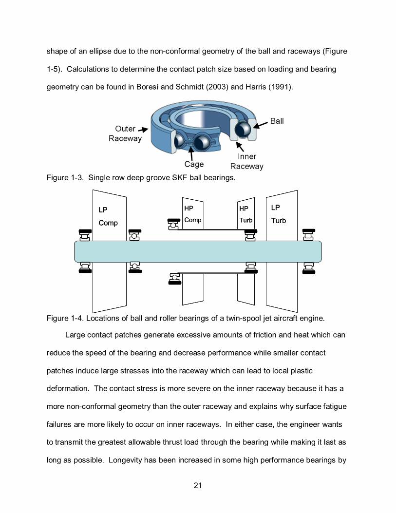
shape of an ellipse due to the non-conformal geometry of the ball and raceways (Figure
1-5). Calculations to determine the contact patch size based on loading and bearing
geometry can be found in Boresi and Schmidt (2003) and Harris (1991).
Figure 1-3. Single row deep groove SKF ball bearings.
LP
Comp
LP
Turb
HP
Turb
HP
CompLP
Comp
LP
Turb
HP
Turb
HP
Comp
Figure 1-4. Locations of ball and roller bearings of a twin-spool jet aircraft engine.
Large contact patches generate excessive amounts of friction and heat which can
reduce the speed of the bearing and decrease performance while smaller contact
patches induce large stresses into the raceway which can lead to local plastic
deformation. The contact stress is more severe on the inner raceway because it has a
more non-conformal geometry than the outer raceway and explains why surface fatigue
failures are more likely to occur on inner raceways. In either case, the engineer wants
to transmit the greatest allowable thrust load through the bearing while making it last as
long as possible. Longevity has been increased in some high performance bearings by

22
using case hardened, stainless steel raceways and ceramic balls. The stainless steel
raceways and ceramic balls resist corrosion. Ceramic balls also have lower densities,
exert lower centrifugal forces, have higher hardness which prevents wear, and perform
better in “oil-out” conditions than steel balls.
Figure 1-5. Deformation due to contact forces between ball and raceways occurs in the form of elliptical contact patches. (Hamrock, 1981).
Bearing Fatigue Failure
Regardless of these benefits, bearings cannot escape the deleterious effects
caused by Foreign Object Debris (FOD), material fatigue, improper handling and
installation, or excessive loading. FOD can cause scratches or dents on the surfaces of
the balls or raceways which act as stress risers and lead to crack formation and crack
growth with continued operation. These cracks eventually liberate surface material and
create a small pit or spall (Figure 1-6.B). Spalls can also be initiated by rolling contact
fatigue that occurs within the ball track of the bearing raceway. Here, local cyclic
plasticity can occur around stress risers in the material microstructure such as
imperfections or carbides in the bearing steel. Similarly, local cracks can form and
grow at these locations with continued operation and lead to surface spalls. This
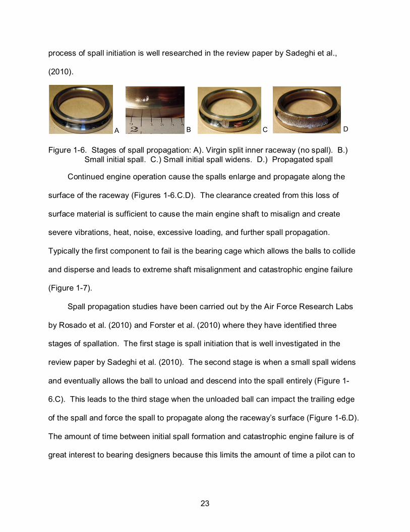
23
process of spall initiation is well researched in the review paper by Sadeghi et al.,
(2010).
A B C D
Figure 1-6. Stages of spall propagation: A). Virgin split inner raceway (no spall). B.) Small initial spall. C.) Small initial spall widens. D.) Propagated spall
Continued engine operation cause the spalls enlarge and propagate along the
surface of the raceway (Figures 1-6.C.D). The clearance created from this loss of
surface material is sufficient to cause the main engine shaft to misalign and create
severe vibrations, heat, noise, excessive loading, and further spall propagation.
Typically the first component to fail is the bearing cage which allows the balls to collide
and disperse and leads to extreme shaft misalignment and catastrophic engine failure
(Figure 1-7).
Spall propagation studies have been carried out by the Air Force Research Labs
by Rosado et al. (2010) and Forster et al. (2010) where they have identified three
stages of spallation. The first stage is spall initiation that is well investigated in the
review paper by Sadeghi et al. (2010). The second stage is when a small spall widens
and eventually allows the ball to unload and descend into the spall entirely (Figure 1-
6.C). This leads to the third stage when the unloaded ball can impact the trailing edge
of the spall and force the spall to propagate along the raceway’s surface (Figure 1-6.D).
The amount of time between initial spall formation and catastrophic engine failure is of
great interest to bearing designers because this limits the amount of time a pilot can to

24
return to safety once an engine bearing begins to spall. Engineers would like to design
bearings with slower spall propagation rates or bearings that don’t spall-propagate at all.
Figure 1-7. Clearance created by spall allows engine shaft to misalign.
As expected, different bearing materials will not have the same spall propagation
characteristics. This was observed in Rosado et al. (2010) where scaled down versions
of the bearings used in the actual aircraft engines were all spall-propagated in controlled
experiments. The bearings were 208 size (40 mm) bore split inner ring raceways with
12.7 mm (0.5 in) diameter balls.
The bearings were thrust loaded in a custom rig by a hydraulic loading cylinder
and attached to an external motor shaft that rotated at a constant 10,000 rpm (Figure 1-
8). Band heaters maintained a constant bearing temperature of 131ºC. Their study
investigated 52100, M50 through-hardened, and M50 NiL case hardened bearing
steels. Their material compositions are shown in Table 1-1. M50 NiL is a low carbon,
high nickel steel that is case hardened.
The M50 and M50 NiL bearings are paired with ceramic silicon nitride balls
whereas the 52100 bearing used 52100 steel balls. Brand new bearings and bearings
that had been subjected to millions of loading cycles were both used in their study to
see if initial rolling contact fatigue affected spall propagation rate.

25
Table 1-1. Material composition of primary alloying elements for the bearing steels in this study. (Rosado et al., 2010), (AMS-Aerospace Material Specification)
Figure 1-8. Bearing test rig for life-endurance and spall propagation bearings at AFRL.
(Rosado et al., 2010).
Figure 1-9 taken from Rosado et al. (2010) shows the rate of mass loss from the
raceway surface of all three types of bearings as a function of stress cycles during spall
propagation. The surfaces of these new bearing raceways were indented with Rockwell
C indents to act as stress risers, initiate fatigue cracks during bearing operation, and
reduce the amount of time to spall initiation. The bearings were inserted into the test rig
and operated at a maximum contact pressure of 2.41 GPa (as seen on the virgin
raceway surface). The mass loss from the spalled bearing was detected by an oil
debris monitor (ODM) and the average sizes of the spalled particles were on the order
of 100 µm (Rosado et al., 2010). The 52100 bearing steel had the shortest amount of
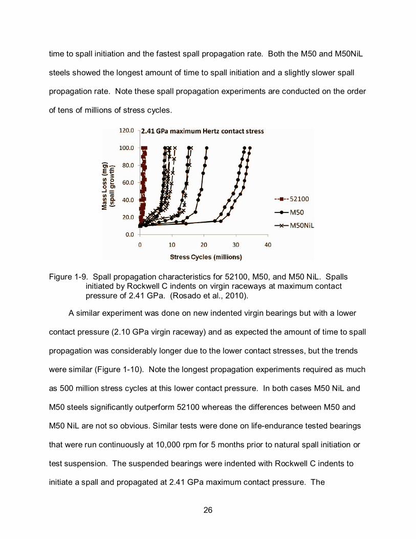
26
time to spall initiation and the fastest spall propagation rate. Both the M50 and M50NiL
steels showed the longest amount of time to spall initiation and a slightly slower spall
propagation rate. Note these spall propagation experiments are conducted on the order
of tens of millions of stress cycles.
Figure 1-9. Spall propagation characteristics for 52100, M50, and M50 NiL. Spalls initiated by Rockwell C indents on virgin raceways at maximum contact pressure of 2.41 GPa. (Rosado et al., 2010).
A similar experiment was done on new indented virgin bearings but with a lower
contact pressure (2.10 GPa virgin raceway) and as expected the amount of time to spall
propagation was considerably longer due to the lower contact stresses, but the trends
were similar (Figure 1-10). Note the longest propagation experiments required as much
as 500 million stress cycles at this lower contact pressure. In both cases M50 NiL and
M50 steels significantly outperform 52100 whereas the differences between M50 and
M50 NiL are not so obvious. Similar tests were done on life-endurance tested bearings
that were run continuously at 10,000 rpm for 5 months prior to natural spall initiation or
test suspension. The suspended bearings were indented with Rockwell C indents to
initiate a spall and propagated at 2.41 GPa maximum contact pressure. The
27
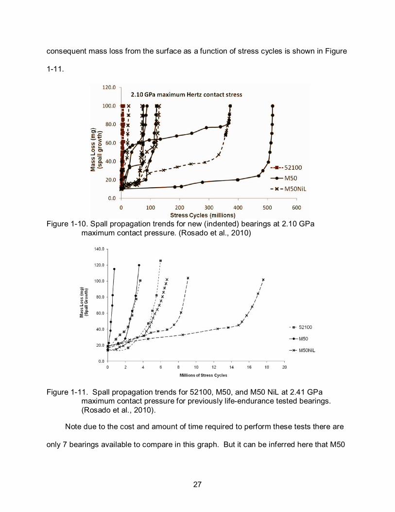
consequent mass loss from the surface as a function of stress cycles is shown in Figure
1-11.
Figure 1-10. Spall propagation trends for new (indented) bearings at 2.10 GPa
maximum contact pressure. (Rosado et al., 2010)
Figure 1-11. Spall propagation trends for 52100, M50, and M50 NiL at 2.41 GPa maximum contact pressure for previously life-endurance tested bearings. (Rosado et al., 2010).
Note due to the cost and amount of time required to perform these tests there are
only 7 bearings available to compare in this graph. But it can be inferred here that M50

28
NiL out performed the other bearing materials in this study as seen by its longer time to
spall growth and slower spall propagation rate. Interestingly, the spall propagation rate
for M50 increased for the life-endurance tested bearings. This suggests that spalls
propagate faster and sooner for M50 bearings that have been in service for a
considerable time.
The fracture toughness of the case hardened layer of M50 NiL is lower than its
core region and M50 through-hardened steel, but close to that of 52100 (Table 1-2).
However, the spall propagation characteristics of M50 NiL are similar to M50 and
superior to 52100 when compared for the virgin indented bearings.
Table 1-2. Mode I fracture toughness of bearing steels in this study. (Rosado et al., 2010).
Material Reference Material Reference
(1989)(1985)(1985)(1985)
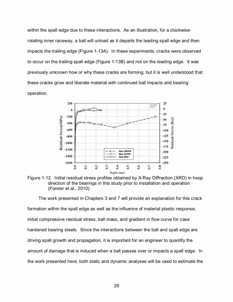
This may be a result of the initial residual compressive stresses that exist within
the case hardened layer of M50 NiL (and not in M50 or 52100) which retard crack
formation and growth and leads to slower spall propagation trends. The initial residual
stresses as a function of depth for these steels are shown in Figure 1-12 and were
obtained by X-Ray Diffraction techniques described in more detail in Forster et al.
(2010). Note the large residual compressive stresses at the surface are due to the final
finishing of the bearing prior to installation and operation, but decrease to zero below a
depth of only 10µm. The actual dynamics of the interactions between a ball and
raceway spall are very complicated, but it is clear that severe damage is occurring
29
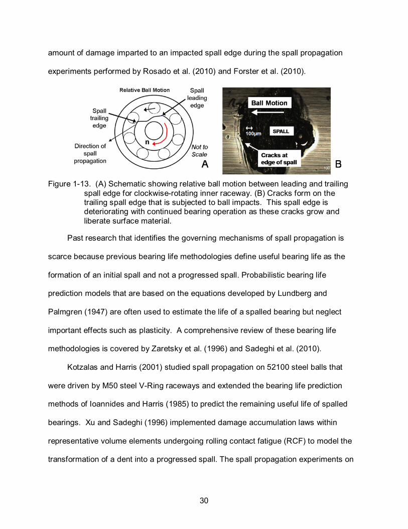
within the spall edge due to these interactions. As an illustration, for a clockwise-
rotating inner raceway, a ball will unload as it departs the leading spall edge and then
impacts the trailing edge (Figure 1-13A). In these experiments, cracks were observed
to occur on the trailing spall edge (Figure 1-13B) and not on the leading edge. It was
previously unknown how or why these cracks are forming, but it is well understood that
these cracks grow and liberate material with continued ball impacts and bearing
operation.
Figure 1-12. Initial residual stress profiles obtained by X-Ray Diffraction (XRD) in hoop
direction of the bearings in this study prior to installation and operation (Forster et al., 2010).
The work presented in Chapters 3 and 7 will provide an explanation for this crack
formation within the spall edge as well as the influence of material plastic response,
initial compressive residual stress, ball mass, and gradient in flow curve for case
hardened bearing steels. Since the interactions between the ball and spall edge are
driving spall growth and propagation, it is important for an engineer to quantify the
amount of damage that is induced when a ball passes over or impacts a spall edge. In
the work presented here, both static and dynamic analyses will be used to estimate the
30
amount of damage imparted to an impacted spall edge during the spall propagation
experiments performed by Rosado et al. (2010) and Forster et al. (2010).
Figure 1-13. (A) Schematic showing relative ball motion between leading and trailing
spall edge for clockwise-rotating inner raceway. (B) Cracks form on the trailing spall edge that is subjected to ball impacts. This spall edge is deteriorating with continued bearing operation as these cracks grow and liberate surface material.
Past research that identifies the governing mechanisms of spall propagation is
scarce because previous bearing life methodologies define useful bearing life as the
formation of an initial spall and not a progressed spall. Probabilistic bearing life
prediction models that are based on the equations developed by Lundberg and
Palmgren (1947) are often used to estimate the life of a spalled bearing but neglect
important effects such as plasticity. A comprehensive review of these bearing life
methodologies is covered by Zaretsky et al. (1996) and Sadeghi et al. (2010).
Kotzalas and Harris (2001) studied spall propagation on 52100 steel balls that
were driven by M50 steel V-Ring raceways and extended the bearing life prediction
methods of Ioannides and Harris (1985) to predict the remaining useful life of spalled
bearings. Xu and Sadeghi (1996) implemented damage accumulation laws within
representative volume elements undergoing rolling contact fatigue (RCF) to model the
transformation of a dent into a progressed spall. The spall propagation experiments on

31
tapered roller bearings by Hoeprich (1992) highlighted the randomness inherent to spall
propagation and its unknown governing mechanisms. A further investigation is needed
to better understand these governing mechanisms and will be presented in this
dissertation.
An outline of the following chapters and objectives are presented here:
• The governing mechanisms of spall propagation will be investigated here through a series of static and dynamic analyses of contact interactions between ball and spall edge. The bearing geometry and operating conditions of (Rosado et al.] will be simulated in finite element models to determine the critical stresses and strains that develop from these interactions in Chapters 2, 3, and 7.
• The plastic response of the case hardened region is unknown for most bearing steels. The material properties of graded materials such as case hardened P675 and M50NiL steels will be determined from a new indentation method presented in Chapters 5 and 6, which relies on the concept of a material-dependent representative plastic strain and indentation forward analysis presented in Chapter 4.
• A new reverse analysis that determines the flow curve of a material based on its measured increase in hardness within a zone of plastic deformation is presented in Chapter 6 and applied to finding the material properties of graded materials when the core properties are unknown initially.
• The material properties of plastically graded M50 NiL are used in a similar dynamic spall model of Chapter 3 to determine if its gradation in plastic response and initial residual stress affect the amount of damage induced by a ball impact on a spall edge in Chapter 7. The effects of surface hardness and ball mass will also be considered.
32
CHAPTER 2 STATIC ANALYSIS OF INITIAL SPALL WIDENING
Motivation and Validation of Finite Element Model
As a first attempt to better understand the governing mechanisms of spall
propagation, a static analysis will investigate stage 2 initial spall widening (Figure 1-5.B
and 1-5.C) since stage 1 spall initiation is well described by Sadeghi et al. (2010). The
magnitude and distribution of the stresses within a spall edge when a ball passes over a
spall are unknown but will be determined here through finite element modeling. Spall
size, ball load, and the location of a ball over a spall are expected to affect the
magnitude and distribution of the stresses within the spall edge. It is also unknown
initially whether linear elastic deformation takes place or if the spall edge plastically
deforms during operation.
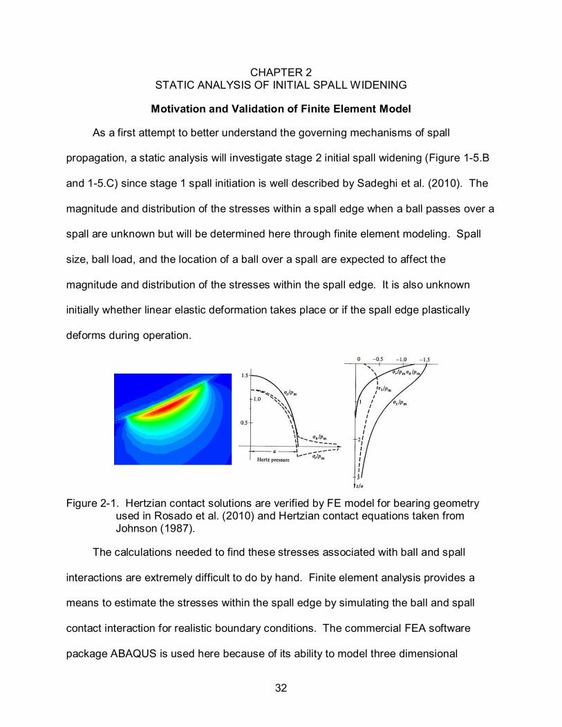
Figure 2-1. Hertzian contact solutions are verified by FE model for bearing geometry
used in Rosado et al. (2010) and Hertzian contact equations taken from Johnson (1987).
The calculations needed to find these stresses associated with ball and spall
interactions are extremely difficult to do by hand. Finite element analysis provides a
means to estimate the stresses within the spall edge by simulating the ball and spall
contact interaction for realistic boundary conditions. The commercial FEA software
package ABAQUS is used here because of its ability to model three dimensional
33
geometries and include plasticity effects. This analysis does not attempt to optimize a
specific numerical solver or create its own finite element code, but will rather apply the
tools that already exist to solve a complex problem.
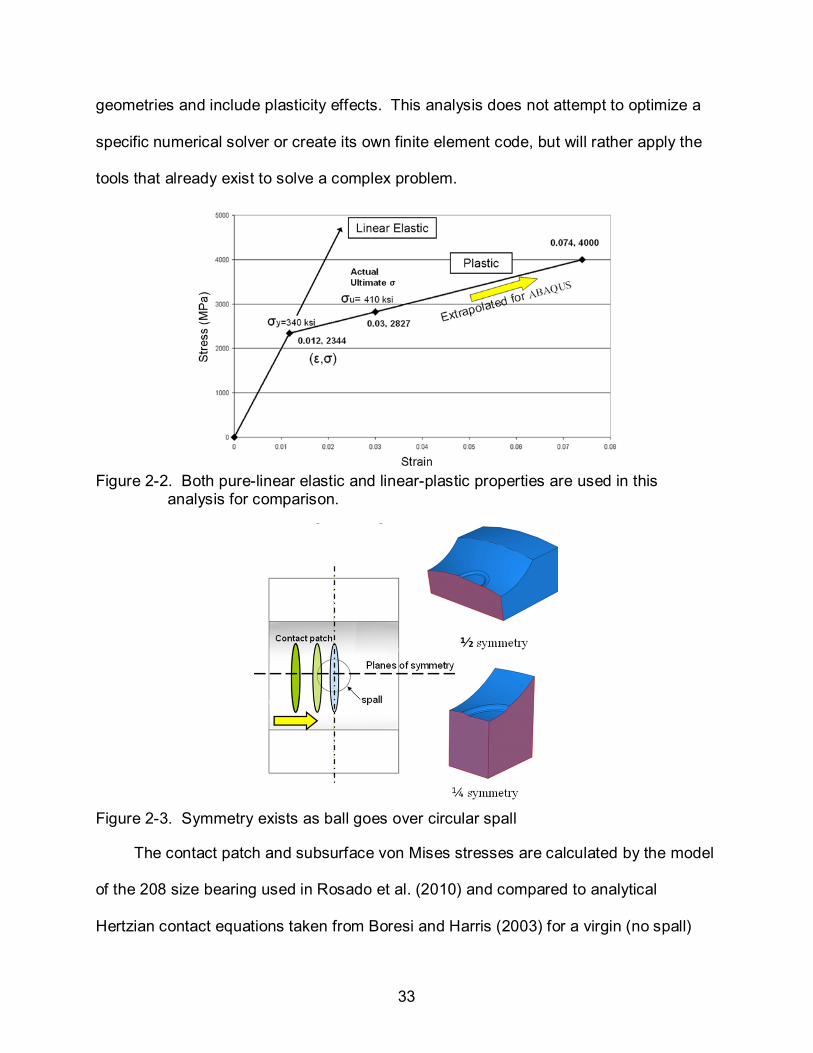
Figure 2-2. Both pure-linear elastic and linear-plastic properties are used in this
analysis for comparison.
Figure 2-3. Symmetry exists as ball goes over circular spall
The contact patch and subsurface von Mises stresses are calculated by the model
of the 208 size bearing used in Rosado et al. (2010) and compared to analytical
Hertzian contact equations taken from Boresi and Harris (2003) for a virgin (no spall)
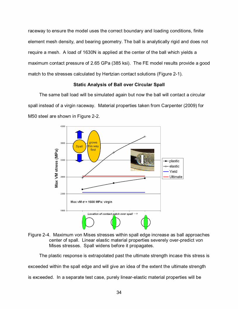
34
raceway to ensure the model uses the correct boundary and loading conditions, finite
element mesh density, and bearing geometry. The ball is analytically rigid and does not
require a mesh. A load of 1630N is applied at the center of the ball which yields a
maximum contact pressure of 2.65 GPa (385 ksi). The FE model results provide a good
match to the stresses calculated by Hertzian contact solutions (Figure 2-1).
Static Analysis of Ball over Circular Spall
The same ball load will be simulated again but now the ball will contact a circular
spall instead of a virgin raceway. Material properties taken from Carpenter (2009) for
M50 steel are shown in Figure 2-2.
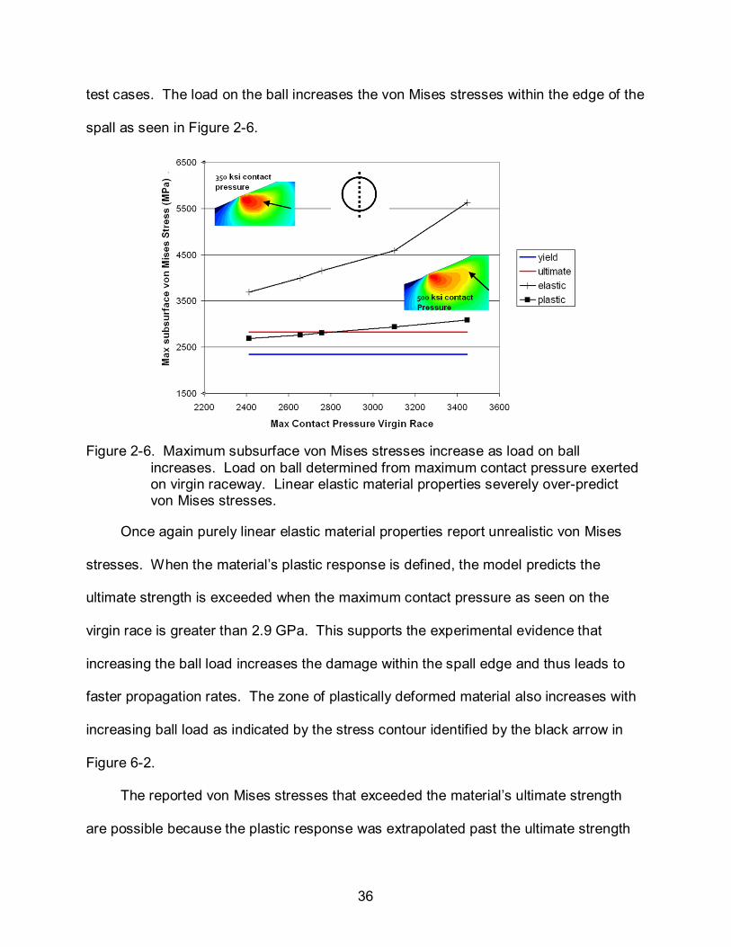
Figure 2-4. Maximum von Mises stresses within spall edge increase as ball approaches
center of spall. Linear elastic material properties severely over-predict von Mises stresses. Spall widens before it propagates.
The plastic response is extrapolated past the ultimate strength incase this stress is
exceeded within the spall edge and will give an idea of the extent the ultimate strength
is exceeded. In a separate test case, purely linear-elastic material properties will be

35
assigned to the spall’s edge to see by how much they over-predict the von Mises
stresses. Symmetry is taken into account in the model geometry in all cases as seen in
Figure 2-3. The maximum von Mises stresses within the edge of the spall are
calculated as a ball goes over the spall at three locations in Figure 2-4.
Figure 2-5. Cross-sections of von Mises stresses within spall edge as ball approaches
spall center.
Linear elastic material properties give unrealistic results as the stresses are
severely over-predicted, whereas when the plastic response is defined, results show
that the stresses are high enough to yield the spall edge. Intuitively, the stresses
increase as the ball approaches the spall center as there is less material available to
support the ball. Subsurface contours of these stresses are shown in Figure 2-5. The
stresses are highest when the ball is over the center of a circular spall, thus more
damage in induced at this location and causes the spall to widen before it propagates
as seen in experiments. Since the stresses are the highest when ball is directly over the
center of a circular spall, this will be treated as the worst case scenario in the next two
36
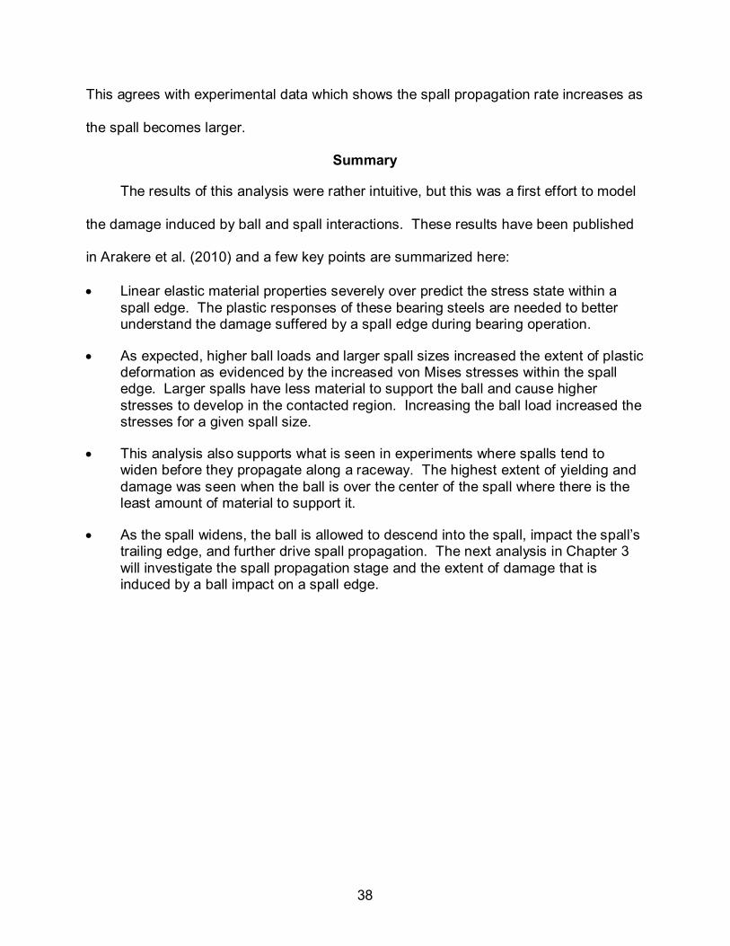
test cases. The load on the ball increases the von Mises stresses within the edge of the
spall as seen in Figure 2-6.
Figure 2-6. Maximum subsurface von Mises stresses increase as load on ball
increases. Load on ball determined from maximum contact pressure exerted on virgin raceway. Linear elastic material properties severely over-predict von Mises stresses.
Once again purely linear elastic material properties report unrealistic von Mises
stresses. When the material’s plastic response is defined, the model predicts the
ultimate strength is exceeded when the maximum contact pressure as seen on the
virgin race is greater than 2.9 GPa. This supports the experimental evidence that
increasing the ball load increases the damage within the spall edge and thus leads to
faster propagation rates. The zone of plastically deformed material also increases with
increasing ball load as indicated by the stress contour identified by the black arrow in
Figure 6-2.
The reported von Mises stresses that exceeded the material’s ultimate strength
are possible because the plastic response was extrapolated past the ultimate strength

37
in the model. In reality, the strength of most materials is increased when subjected to
high strain rates which are possible in the small region of a spall edge along with the
high velocity of the moving balls.
Figure 2-7. Maximum subsurface von Mises stresses within spall edge increase as
spall diameter increases. Elastic material properties over-predict von Mises stresses.
As the spall widens there is less material to support the loaded ball which would
lead to higher stresses within the spall edge. This was modeled and the results are
shown in Figure 2-7. Linear elastic material properties give unrealistic stress results
within the edge of the spall. When plasticity is defined, the spall edge is allowed to
plastically deform and the ultimate strength is exceeded for a 4 mm diameter circular
spall for this material and bearing geometry. Thus more damage is induced in the form
of plastic deformation in larger spalls because there is less material to support the ball.
38
This agrees with experimental data which shows the spall propagation rate increases as
the spall becomes larger.
Summary
The results of this analysis were rather intuitive, but this was a first effort to model
the damage induced by ball and spall interactions. These results have been published
in Arakere et al. (2010) and a few key points are summarized here:
• Linear elastic material properties severely over predict the stress state within a spall edge. The plastic responses of these bearing steels are needed to better understand the damage suffered by a spall edge during bearing operation.
• As expected, higher ball loads and larger spall sizes increased the extent of plastic deformation as evidenced by the increased von Mises stresses within the spall edge. Larger spalls have less material to support the ball and cause higher stresses to develop in the contacted region. Increasing the ball load increased the stresses for a given spall size.
• This analysis also supports what is seen in experiments where spalls tend to widen before they propagate along a raceway. The highest extent of yielding and damage was seen when the ball is over the center of the spall where there is the least amount of material to support it.
• As the spall widens, the ball is allowed to descend into the spall, impact the spall’s trailing edge, and further drive spall propagation. The next analysis in Chapter 3 will investigate the spall propagation stage and the extent of damage that is induced by a ball impact on a spall edge.

39
CHAPTER 3 DYNAMIC ANALYSIS OF BALL IMPACT WITH SPALL EDGE
Ball Impact with Spall Edge Drives Propagation
With continued bearing operation, the spall widens to such an extent to allow the
ball to descend into the spall and impact the trailing edge. For a clockwise-spinning
inner raceway and a relatively fixed outer raceway (Figure 3-1), the relative motion of
the balls and inner raceway cause the balls to impact the trailing edge of the spall as it
reestablishes contact between the inner and outer raceways. As a result, spall
propagation is in the same direction as the ball motion relative to the spall edge.
Figure 3-1. Relative ball motion causes ball impact with trailing spall edge
Figure 3-2. Cracks form on spall trailing edge. Typical spall depth is 127µm.
The spall’s trailing edge is defined as the edge that deteriorates with bearing
operation, whereas the spall’s leading edge is a portion of the initial spall and remains
throughout propagation (Figure 3-1). The numerous impacts that occur between the

40
ball and trailing spall edge are thought to be the main driving forces of spall
propagation. Both the leading and trailing edges experience the pinch caused by the
ball’s contact with the inner and outer raceways; however, only the trailing edge is
subjected to ball impacts and deterioration.
Also, significant cracks form only on the spall’s trailing edge (Figures 3-2 and 3-3)
as the spall is propagating. This is another indication that more damage is occurring on
the impacted edge in the form of cracks and not on the leading edge. Continuous ball
impacts encourage these cracks to grow and cause fragments of material to liberate
from the raceway’s surface. The fragments collected by the Oil Debris Monitor (ODM) in
Rosado et al. (2010) were typically the same size as the edge of the spall (100 µm). The
mechanisms that cause these cracks to form were previously unknown, but an
explanation will be given later in this chapter and in Chapter 7.
Figure 3-3. Cracks appear on the spall’s trailing edge
Finite Element Model
The dynamic analysis presented here is unique because it uses finite element
models that include the effects of plasticity to calculate the critical stresses and strains
that develop within a spall edge during and after successive ball impacts. The modeling
results are supported by the locations of cracks along a spall edge. This information will

41
support a plausible scenario of why fatigue spalls propagate. This new finite element
model is similar to the one from the static analysis except now the spall is sufficiently
large enough to allow the ball to completely unload and impact the trailing edge. Actual
bearing dynamics are very complex with interactions between the balls, cage, and
raceways, but are not considered here in interest of time and simplicity. Only a
segment of the inner raceway is modeled and the ball is given a mass and velocity and
allowed to impact the spall edge (Figures 3-4 and 3-6).
Raceway Segment
Spall
Raceway Segment
Spall
Plane of Symmetry
Hoop Direction
Radial Direction
Spall EdgeSpall Edge
Raceway Segment
Spall Depth 127 µm
Figure 3-4. Only segment of inner raceway is modeled.
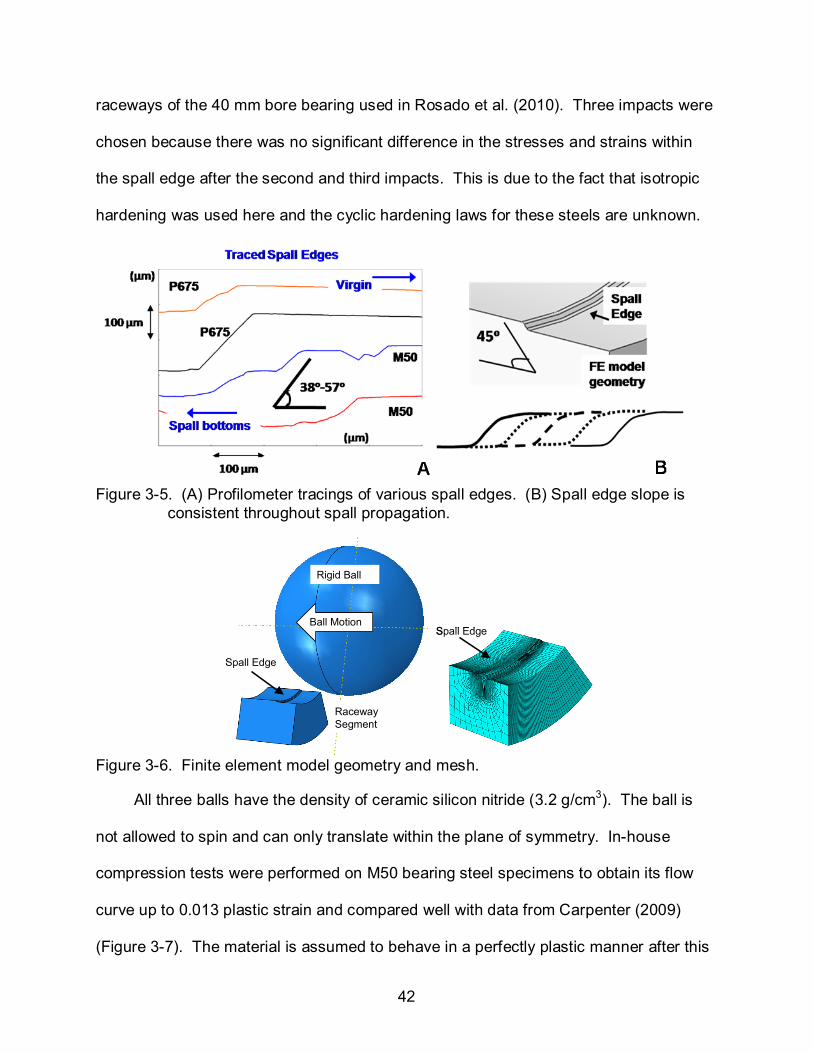
To capture the geometry of the spall edge, profilometer tracings were taken on
propagated spall edges from case hardened Pyrowear 675 (P675) and M50 through
hardened bearing steels (Figure 3-5.A). An average spall slope of 45 degrees was
measured from the four profiles and used in the finite element model geometry (Figure
3-5.B). This edge geometry is consistent during spall propagation regardless of spall
length (Figure 3-5.B).
The finite element model will simulate three successive rigid ball impacts on the
same spall edge at a ball velocity of 15.24 m/s (50 ft/s) (Figure 3-6). The ball velocity is
determined from the kinematics of the known rotational speeds of the cage and
42
raceways of the 40 mm bore bearing used in Rosado et al. (2010). Three impacts were
chosen because there was no significant difference in the stresses and strains within
the spall edge after the second and third impacts. This is due to the fact that isotropic
hardening was used here and the cyclic hardening laws for these steels are unknown.
Figure 3-5. (A) Profilometer tracings of various spall edges. (B) Spall edge slope is
consistent throughout spall propagation.
Spall EdgeSpall Edge
Rigid Ball
Raceway Segment
Spall Edge
Ball Motion
Rigid Ball
Raceway Segment
Spall Edge
Ball MotionBall Motion
Figure 3-6. Finite element model geometry and mesh.
All three balls have the density of ceramic silicon nitride (3.2 g/cm3). The ball is
not allowed to spin and can only translate within the plane of symmetry. In-house
compression tests were performed on M50 bearing steel specimens to obtain its flow
curve up to 0.013 plastic strain and compared well with data from Carpenter (2009)
(Figure 3-7). The material is assumed to behave in a perfectly plastic manner after this

43
strain is reached as observed by the decreasing strain hardening trend obtained from
the compression test. Very hard materials such as bearing steels do not have a large
capacity to strain harden like copper or 303 stainless steel (Lai and Lim, 1991), so a
perfectly plastic assumption is valid here. Also the cyclic hardening properties are
unknown for most bearing steels thus only the monotonic stress strain curve will be
utilized here.
Figure 3-7. Flow curve of M50 steel from in-house compression test
A very fine linear hexahedral mesh is designed around the spall’s edge because
the most critical stresses and strains are forming in this small region (Figure 3-6). The
explicit solver within ABAQUS v6.8-2 was used since this is a transient analysis and has
time-dependent properties (the velocity of the ball). The von Mises (J2) failure criterion,
associative flow rule, and isotropic hardening are appropriate for bearing steels and
implemented here.
Finite Element Model Results
All plots of the finite element model results are close-up images of a spall edge’s
cross-section. The radial stresses during impact were calculated and mostly
compressive as expected (Figure 3-8). The maximum contact pressure between the
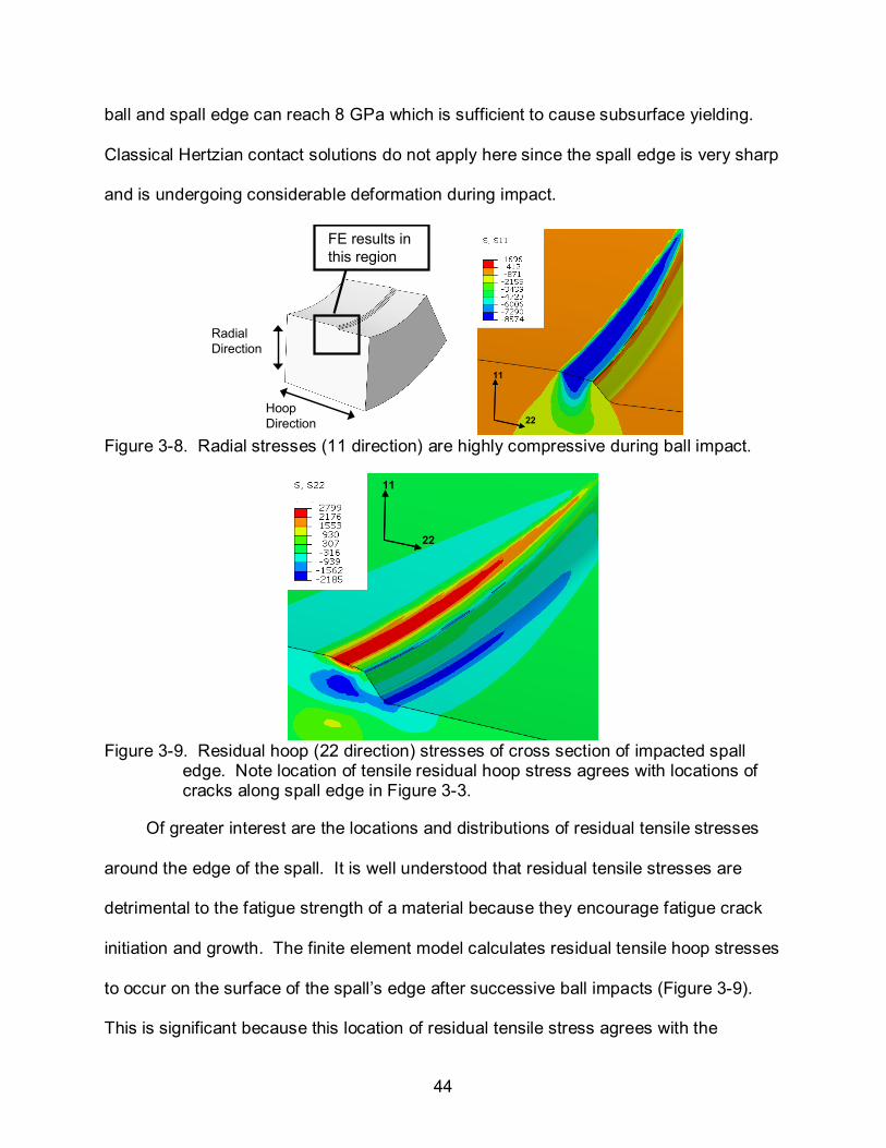
44
ball and spall edge can reach 8 GPa which is sufficient to cause subsurface yielding.
Classical Hertzian contact solutions do not apply here since the spall edge is very sharp
and is undergoing considerable deformation during impact.
FE results in this region
Hoop Direction
Radial Direction
11
22
11
22
Figure 3-8. Radial stresses (11 direction) are highly compressive during ball impact.
11
22
11
22
Figure 3-9. Residual hoop (22 direction) stresses of cross section of impacted spall
edge. Note location of tensile residual hoop stress agrees with locations of cracks along spall edge in Figure 3-3.
Of greater interest are the locations and distributions of residual tensile stresses
around the edge of the spall. It is well understood that residual tensile stresses are
detrimental to the fatigue strength of a material because they encourage fatigue crack
initiation and growth. The finite element model calculates residual tensile hoop stresses
to occur on the surface of the spall’s edge after successive ball impacts (Figure 3-9).
This is significant because this location of residual tensile stress agrees with the
45
locations of cracks around the spall’s edge (Figure 3-3) in the bearings from Rosado et
al. (2010).
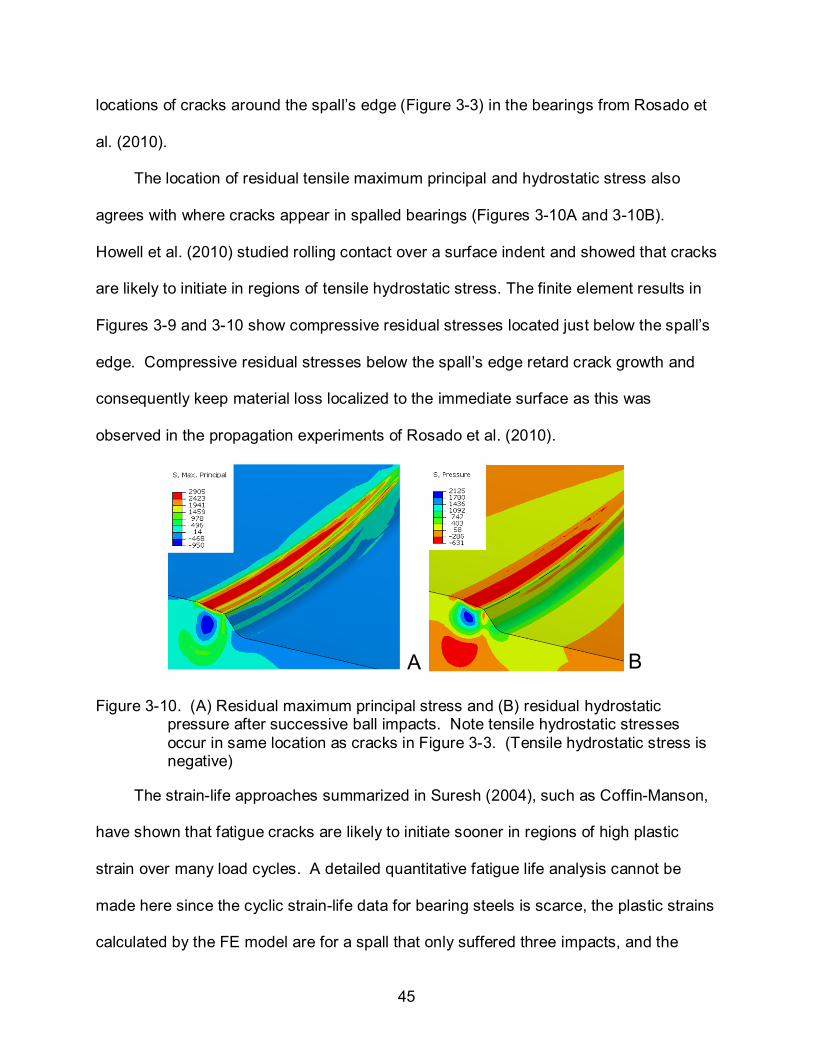
The location of residual tensile maximum principal and hydrostatic stress also
agrees with where cracks appear in spalled bearings (Figures 3-10A and 3-10B).
Howell et al. (2010) studied rolling contact over a surface indent and showed that cracks
are likely to initiate in regions of tensile hydrostatic stress. The finite element results in
Figures 3-9 and 3-10 show compressive residual stresses located just below the spall’s
edge. Compressive residual stresses below the spall’s edge retard crack growth and
consequently keep material loss localized to the immediate surface as this was
observed in the propagation experiments of Rosado et al. (2010).
A B
Figure 3-10. (A) Residual maximum principal stress and (B) residual hydrostatic pressure after successive ball impacts. Note tensile hydrostatic stresses occur in same location as cracks in Figure 3-3. (Tensile hydrostatic stress is negative)
The strain-life approaches summarized in Suresh (2004), such as Coffin-Manson,
have shown that fatigue cracks are likely to initiate sooner in regions of high plastic
strain over many load cycles. A detailed quantitative fatigue life analysis cannot be
made here since the cyclic strain-life data for bearing steels is scarce, the plastic strains
calculated by the FE model are for a spall that only suffered three impacts, and the

46
cyclic plastic strain amplitudes from the FE model are highly dependent on its cyclic
strain hardening law which is also limited for bearing steels. However, as a qualitative
investigation it is worth comparing the distribution of plastic strain within the spall edge
with the location of cracks in the actual bearings to determine if cracks form in the most
damaged region as predicted by the FE model.
The distribution of maximum principal plastic strain is shown in Figure 3-11.
Cracks are likely to follow this path of highly damaged material and aided by the tensile
and compressive residual stresses within the spall. The distribution of maximum
principal plastic strain is also similar to the profilometer tracings of the spall edges
(Figure 3-5). After a fragment of material is liberated from a spall edge, the new spall
edge profile left behind is a close match to the profilometer tracings and the distribution
of maximum principal plastic strain. This process repeats itself and explains why the
spall edge profile does not vary throughout spall propagation.
315 µm
250 µm
315 µm
250 µm
Figure 3-11. Plastic zone size and maximum principal plastic strain contour at spall edge cross section after successive ball impacts. Cracks likely to follow path of most heavily damaged material and leave behind similar spall edge.
Spall edge geometry is expected to influence the calculation of stresses and
strains in the finite element model; however it is shown here that similar residual stress
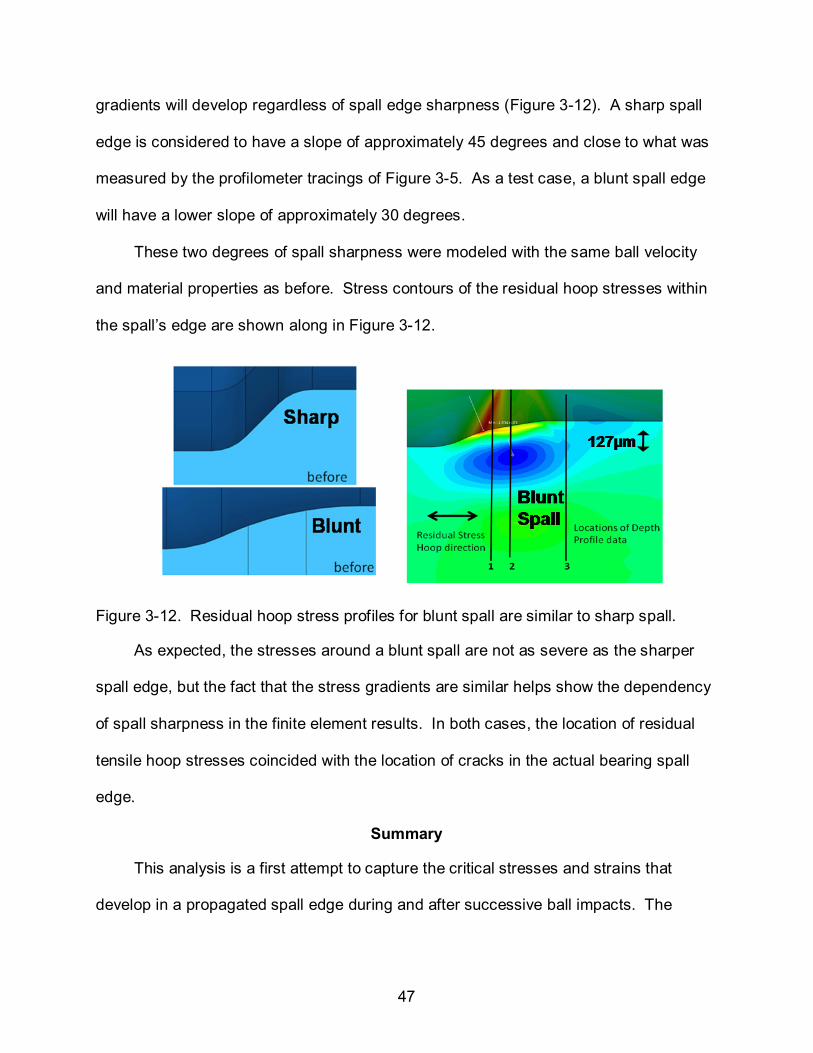
47
gradients will develop regardless of spall edge sharpness (Figure 3-12). A sharp spall
edge is considered to have a slope of approximately 45 degrees and close to what was
measured by the profilometer tracings of Figure 3-5. As a test case, a blunt spall edge
will have a lower slope of approximately 30 degrees.
These two degrees of spall sharpness were modeled with the same ball velocity
and material properties as before. Stress contours of the residual hoop stresses within
the spall’s edge are shown along in Figure 3-12.
Figure 3-12. Residual hoop stress profiles for blunt spall are similar to sharp spall.
As expected, the stresses around a blunt spall are not as severe as the sharper
spall edge, but the fact that the stress gradients are similar helps show the dependency
of spall sharpness in the finite element results. In both cases, the location of residual
tensile hoop stresses coincided with the location of cracks in the actual bearing spall
edge.
Summary
This analysis is a first attempt to capture the critical stresses and strains that
develop in a propagated spall edge during and after successive ball impacts. The

48
results of this analysis have been published in Branch et al. (2010) and the key points
are outlined here:
• It is well understood that residual tensile stresses decrease the fatigue life of a material and correspond to regions of crack initiation Sadeghi et al. (2010). The finite element model determines residual hoop, radial, and hydrostatic tensile stresses to occur within an impacted spall edge at the same locations where cracks are observed in the actual bearings.
• The residual compressive stresses below the trailing edge of the spall retard crack growth and keep material loss localized to the immediate surface as seen in actual bearing surface failures.
• The distribution of maximum principal plastic strain within the spall edge provides a likely path of crack growth which leads to the liberation of material fragments during spall propagation. This is supported by observations that the spall edge shape is consistent throughout propagation and closely matches the distribution of maximum principal plastic strain that is calculated by the model. Qualitative strain-life methodologies predict cracks to initiate in regions of high plastic strain, and cracks appear on spall edges where the finite element model predicts large plastic strain.
• This analysis will be repeated for case hardened M50 NiL, but the plastic response of the plastically-graded, case hardened layer is unknown initially. A new indentation method presented in Chapters 5 and 6 will determine the plastic response of graded materials and will be based on the concept of representative plastic strain and indentation of nongraded materials discussed in more detail in Chapter 4.
49
CHAPTER 4 INDENTATION OF NON-GRADED MATERIALS
Relationship between Hardness and Yield Strength
The plastic response of case hardened bearings steels are needed to better
understand spall propagation that occurs within their case layers. The method of using
indentation hardness measurements and finite element modeling to determine the
plastic response of graded materials such as case-hardened bearing steels must be
validated for non-graded materials first. Parameters such as the representative plastic
strain induced by a Vickers indent must be clarified for simple materials before applying
them to graded materials.
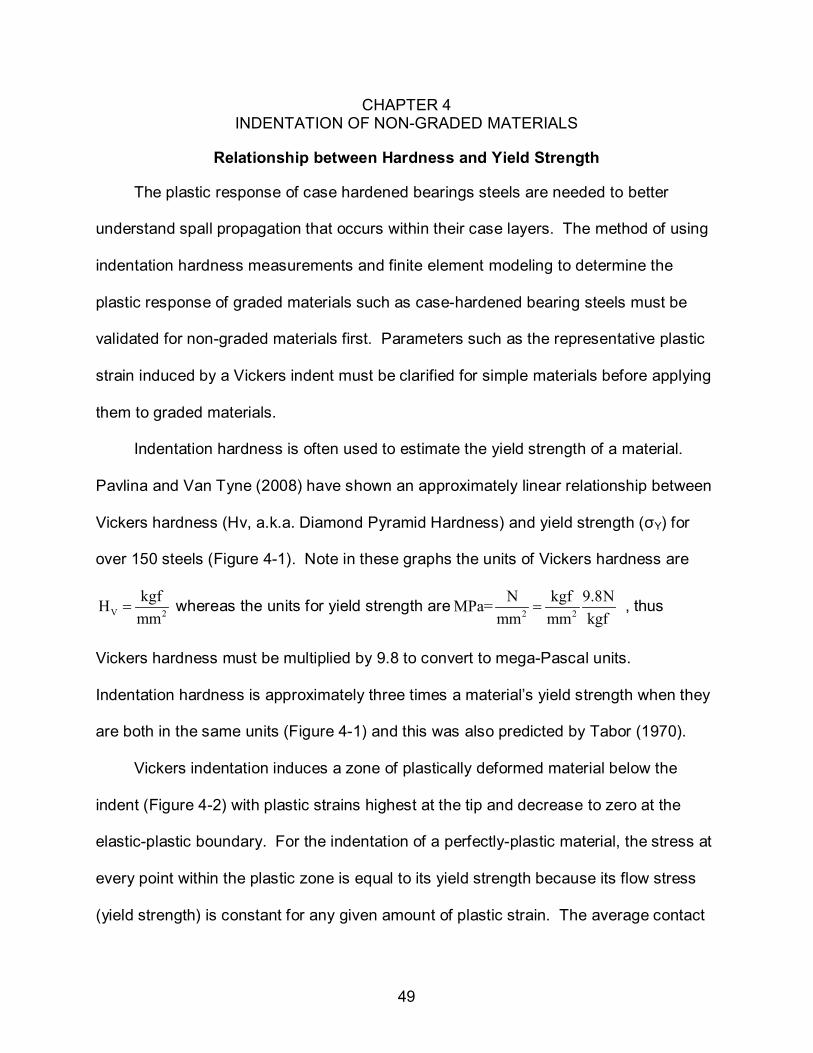
Indentation hardness is often used to estimate the yield strength of a material.
Pavlina and Van Tyne (2008) have shown an approximately linear relationship between
Vickers hardness (Hv, a.k.a. Diamond Pyramid Hardness) and yield strength (σY) for
over 150 steels (Figure 4-1). Note in these graphs the units of Vickers hardness are
V 2
kgfHmm
= whereas the units for yield strength are 2 2
N kgf 9.8NMPa= mm mm kgf
= , thus
Vickers hardness must be multiplied by 9.8 to convert to mega-Pascal units.
Indentation hardness is approximately three times a material’s yield strength when they
are both in the same units (Figure 4-1) and this was also predicted by Tabor (1970).
Vickers indentation induces a zone of plastically deformed material below the
indent (Figure 4-2) with plastic strains highest at the tip and decrease to zero at the
elastic-plastic boundary. For the indentation of a perfectly-plastic material, the stress at
every point within the plastic zone is equal to its yield strength because its flow stress
(yield strength) is constant for any given amount of plastic strain. The average contact

50
pressure (Vickers hardness) needed to plastically deform the material is typically three
times the material’s yield strength as predicted by Tabor (1970). This ratio is called the
constraint factor (C) where for most materials:
3Y
HCσ
= ≈ (4.1)
A B
Figure 4-1. (A) Vickers indenter geometry and (B) the linear relationship between Vickers indentation hardness and Yield strength. (Figures (A) ASM handbook, 2009; (B) Pavlina and Van Tyne, 2008).
Figure 4-2. Vickers hardness is essentially the contact pressure needed to yield the indented material for this specific indenter geometry. Average flow stress within plastic zone is its yield strength for a perfectly plastic material.
For a strain hardening material, relating indentation hardness to yield strength
becomes a bit more complicated. When a strain hardening material undergoes any
type of permanent deformation, its yield strength (flow stress) will increase according to
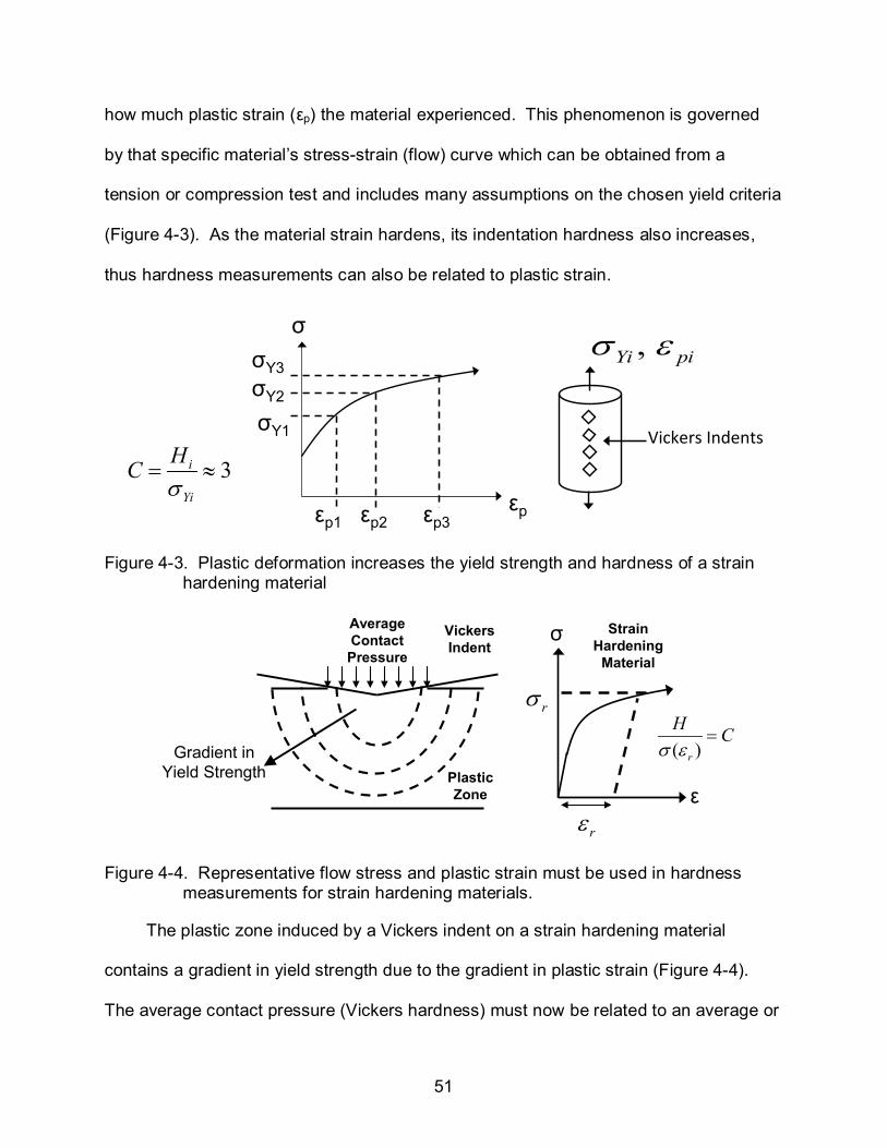
51
how much plastic strain (εp) the material experienced. This phenomenon is governed
by that specific material’s stress-strain (flow) curve which can be obtained from a
tension or compression test and includes many assumptions on the chosen yield criteria
(Figure 4-3). As the material strain hardens, its indentation hardness also increases,
thus hardness measurements can also be related to plastic strain.
σ
εpεp1 εp2 εp3
σY1
σY2
σY3
3i
Yi
HCσ
= ≈
, Yi piσ ε
Vickers Indents
Figure 4-3. Plastic deformation increases the yield strength and hardness of a strain hardening material
Plastic Zone
Strain Hardening
Material
Average Contact Pressure
Vickers Indent
σ
Gradient in Yield Strength
ε
rσ
rε
( )r
H Cσ ε
=
Figure 4-4. Representative flow stress and plastic strain must be used in hardness measurements for strain hardening materials.
The plastic zone induced by a Vickers indent on a strain hardening material
contains a gradient in yield strength due to the gradient in plastic strain (Figure 4-4).
The average contact pressure (Vickers hardness) must now be related to an average or

52
“representative” flow stress within the plastic zone since the stresses closest to the
indent are significantly higher than its yield strength. This representative flow stress
rσ corresponds to a representative plastic strain rε on a material’s flow curve such
that
( )r rσ σ ε= (4.2)
The ratio of hardness to representative flow stress is still close to three for strain
hardening materials:
( ) , 3rH C Cσ ε= ≈ (4.3)
Predicting Increase in Hardness of Strain Hardening Material
A method that predicts the indentation hardness of a plastically-deformed strain-
hardening material was first introduced by Tabor (1970) where he recorded the increase
in Vickers hardness (Hv) of strain hardening materials with known amounts of initial
plastic deformation ( oε ) (also written as ipε throughout this document). Tabor (1970)
discovered that a Vickers indent plastically deforms (and strain hardens) a region that
has an initial state of plastic deformation. Thus the average or representative flow
stress within the plastic zone will always be greater than the initial yield strength prior to
indentation. An example of this is shown next.
Tabor (1970) utilized five specimens of mild steel and annealed copper deformed
to various amounts of plastic strain εo (Table 4-1). The measured Vickers hardness of
these deformed specimens is shown in the “Observed Vickers Hardness Number”
column as a function of initial plastic strain (initial deformation column). The

53
representative plastic strain rε induced by the indent (0.08) was added to the initial
plastic deformation oε of every specimen ( oε + 8 % column). The flow stress
corresponding to this total strain was found on the known flow curve (“Y” column). This
flow stress was then multiplied by 2.9 or 3 and compared well to the measured
hardness values (“cY” column).
Table 4-1. Tabor (1970) measured the increase in hardness of plastically deformed strain hardened materials. A representative strain of 8% was used to account for strain hardening induced by a Vickers indent.
Note that the eight % representative plastic strain is somewhat of a statistical fit
and not based on the actual plastic strain gradient within the plastic zone of a Vickers
indent. His method shown in Table 4-1 can be best summarized by the equation
( )ip rH Cσ ε ε= + (4.4)
and this also predicts the hardness of materials with no initial plastic deformation (virgin
materials) when 0ipε → and yields ( )rH Cσ ε= as shown in equation 4.3. This
method to predict hardness is frequently used for both metals and ceramics.
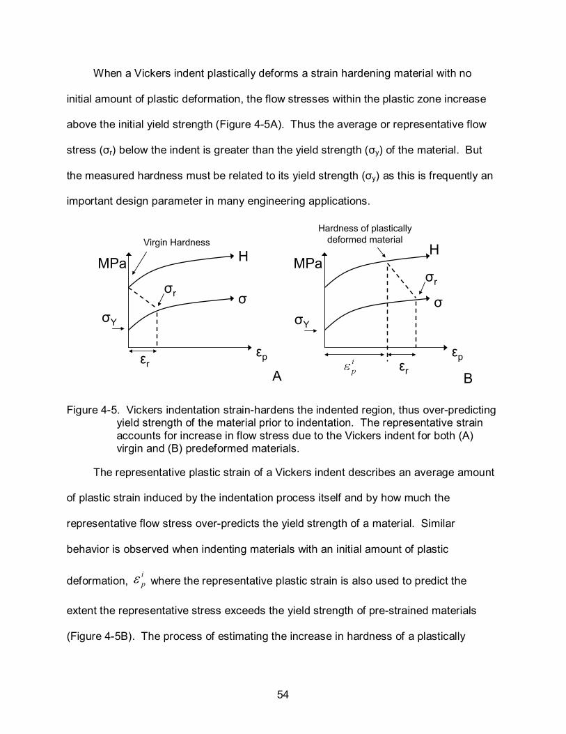
54
When a Vickers indent plastically deforms a strain hardening material with no
initial amount of plastic deformation, the flow stresses within the plastic zone increase
above the initial yield strength (Figure 4-5A). Thus the average or representative flow
stress (σr) below the indent is greater than the yield strength (σy) of the material. But
the measured hardness must be related to its yield strength (σy) as this is frequently an
important design parameter in many engineering applications.
MPa
εp
H
σ
εr
σr
MPa
εp
H
σ
εr
σr
σY
Virgin HardnessHardness of plastically
deformed material
(a) (b)
σY
MPa
εp
H
σ
εr
σr
MPa
εp
H
σ
εr
σr
σY
Virgin HardnessHardness of plastically
deformed material
(a) (b)
σY
A B
Figure 4-5. Vickers indentation strain-hardens the indented region, thus over-predicting yield strength of the material prior to indentation. The representative strain accounts for increase in flow stress due to the Vickers indent for both (A) virgin and (B) predeformed materials.
The representative plastic strain of a Vickers indent describes an average amount
of plastic strain induced by the indentation process itself and by how much the
representative flow stress over-predicts the yield strength of a material. Similar
behavior is observed when indenting materials with an initial amount of plastic
deformation, ipε where the representative plastic strain is also used to predict the
extent the representative stress exceeds the yield strength of pre-strained materials
(Figure 4-5B). The process of estimating the increase in hardness of a plastically
55
deformed material when its flow curve is known is called a forward analysis. The
opposite case when one wishes to predict a flow curve based on known measured
indentation hardness values is called a reverse analysis and more difficult to perform. A
new reverse analysis will be shown in Chapter 6 and will be applied to determining the
plastic response of graded materials. Many different forward and reverse analyses
have been proposed since Tabor, and one of the most controversial topics in these
methods is how the representative plastic strain induced by an indent is defined and
calculated.
Representative Plastic Strain Background
Representative plastic strain is also frequently called offset strain, average strain,
and characteristic strain in the literature. Previous indentation methods that determine
the plastic response of materials cannot agree on a single value for representative
strain, but all agree that it is essentially a plastic strain induced by an indent that is used
to relate indentation hardness to yield strength (Tabor, 1970; Chollacoop and
Ramamurty, 2005; Sonmez and Demir, 2007). With advances in technology came the
advent of instrumented indentation devices that could relate indentation response to a
material’s plastic response. Instrumented indentation devices essentially measure the
indent load (P) as a function of indent depth (δ) continuously throughout the indentation
process (Figure 4-6). This relationship is parabolic for most materials and the resulting
loading curvature (Cv) can be unique to specific material properties.
The much referenced paper by Dao et al. (2001) predicted a material’s elastic and
plastic response based on its instrumented indentation loading curvature, Cv. Dao et al.
(2001) created a set of dimensionless functions to characterize the indentation

56
response of a given range of material properties. This was done by simulating Vickers
indentation of these materials and recording the loading curvatures Cv from
P=Cvδ2 (4.5)
during indentation. The loading curvatures were plotted against the reduced modulus
and both parameters were normalized with respect to a representative stress (a function
of representative strain). By minimizing the error of this relationship using a least
squares algorithm, a value of the representative strain of 0.033 was determined to make
this relationship independent of the strain hardening exponent, n, of the power law
plastic response
nKσ ε= (4.6)
where K is the strength coefficient.
PP
2vP C δ=
Figure 4-6. Schematic of typical instrumented indentation loading curve. P-indent load, δ-indent depth, and Cv-loading curvature.
Note this 0.033 representative plastic strain is quite different from Tabor’s 0.08,
and based on the statistical fits of a chosen range of material properties. Many
methods similar to Dao et al. (2001) soon followed, most of which used different values
for representative plastic strain. Bucaille et al. (2003) extended the method of Dao et al.
(2001) to conical indenters with different included angles and used two indenters to
characterize the flow curve of a material based on its instrumented-indentation
57
response. Friction effects were shown to be negligible for included angles greater than
60 degrees and that the representative strain is dependent only on choice of indenter.
Ogasawara et al. (2005) extended the method of Dao et al. (2001) to three conical
indenters of different included angles, determined that the range of material properties
used by Dao et al. (2001) were too narrow, and that the representative strain of Dao et
al. (2001) was not associated with elastic or plastic deformation. Ogasawara et al.
(2005) proposed a new definition of representative strain that accounts for the biaxial
nature of plastic strain common in Vickers indentation plastic zones and that its value is
0.0115 for the 70.3 degree included cone angle that is used to represent Berkovich and
Vickers indenters. Ogasawara et al., (2006) created new fitting functions derived from
the elastic and plastic work of the indentation response for a single indenter method
while maintaining the same rε as Ogasawara et al. (2005). Chollacoop et al. (2005)
showed how initial plastic deformation affects the indentation loading curvature and that
the method of Dao et al. (2001) can be used to predict flow curves using two different
indenters on strain hardening materials. Cao and Huber (2006) showed that the
representative strain is dependent on material properties and reported rε values in the
range 0.023 to 0.095.
Methods that did not use instrumented indentation also utilized different values for
representative plastic strain. Johnson (1987) reported a representative strain of 0.07
based on the boundary of the large hydrostatic stress “core” directly beneath the tip of a
sharp indent. Chaudhri (1998) suggested that the representative strain should be the
maximum plastic strain in the plastic zone of a Vickers indent and reported values
between 0.25 and 0.36. However much higher plastic strains have been observed to
58
occur (Dao et al., 2001; Bucaille and Felder, 2002; Bucaille et al., 2003). Tekkaya
(2000) proposed a value of 0.112rε = based on their experiments that predicted the
plastic strain and increase in hardness associated with extrusion processes. Antunes et
al. (2007) also expressed a need to have a material dependent representative strain
and reported rε values to range between 0.034 and 0.042.
Most of the previous definitions of representative plastic strain were not based on
a physical and measurable quantity. Rather, these parameters were calculated from
curve fitting and statistical fits of the indentation responses of a certain range of material
properties. The “representative strain” is really a misnomer in that it is not
“representing” the actual plastic deformation within the plastic zone of a Vickers indent.
Chaudhri (1998) has dubbed Tabor’s 8% strain an “undefined global value” whereas the
0.033 representative strain proposed by Dao et al. (2001) has been called a
“mathematical trick” and has “no physical basis” (Ogasawara et al., 2005).
These methods are trying to find a universal value for representative strain that
works for all materials. However the plastic strain induced by a Vickers indent is highly
dependent on the indented material’s inherent resistance to plastic deformation which is
typically characterized by the strain hardening exponent. A universal value for
representative plastic strain is not expected to work for a wide range of materials.
These methods also rely heavily on the use of instrumented indentation devices in
their characterization of material properties. These machines can be expensive, hard to
calibrate (VanLandingham, 2003), and may not be available at certain research labs or
universities. The unloading curve can estimate the strain hardening exponent and
elastic modulus, but uncertainties have been identified in determining the unloading

59
slope (VanLandingham, 2003). The previous methods also require the running of many
finite element models along with numerous dimensionless functions to characterize a
given range of material properties which may not be all-encompassing. In fact some
research has shown that two different materials can produce the same indentation
loading curvature in single indenter methodologies (Chollacoop et al., 2003).
Average Volumetric Plastic Strain as Representative Plastic Strain
There has been a recent call to simplify indentation methodologies that are used to
predict the plastic response of materials (Baxevani and Giannakopoulos, 2009). New
methods are desired that do not require many FE models, instrumented indentation
equipment, or multiple indenters. The method presented here is a forward analysis that
meets these criteria and uses a representative plastic strain that is a calculable quantity
of the plastic strain induced by an indent. The representative plastic strain used in this
analysis will be the average volumetric equivalent plastic strain of a Vickers indent’s
plastic zone. This average plastic strain is independent of material yield strength and
elastic modulus (Jayaraman et al., 1998).
The average equivalent plastic strain is defined as
i ir
i
VVε
ε = ∑∑
(4.7)
where εi is the equivalent plastic strain:
( ) ( ) ( )2 2 2
1 2 2 3 1 32
3i p p p p p pε ε ε ε ε ε ε= − + − + − (4.8)
at the centroid of an elemental volume, iV . It has been suggested that this average
strain is not a valid representative strain because it is dependent on the strain hardening
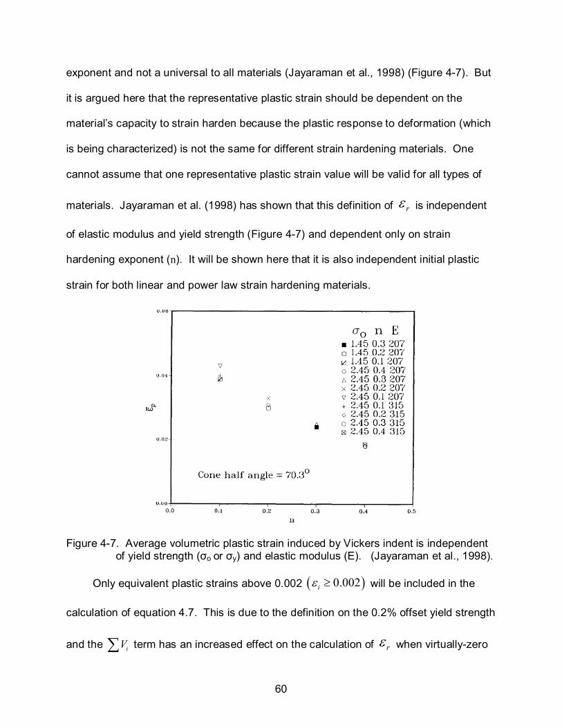
60
exponent and not a universal to all materials (Jayaraman et al., 1998) (Figure 4-7). But
it is argued here that the representative plastic strain should be dependent on the
material’s capacity to strain harden because the plastic response to deformation (which
is being characterized) is not the same for different strain hardening materials. One
cannot assume that one representative plastic strain value will be valid for all types of
materials. Jayaraman et al. (1998) has shown that this definition of rε is independent
of elastic modulus and yield strength (Figure 4-7) and dependent only on strain
hardening exponent (n). It will be shown here that it is also independent initial plastic
strain for both linear and power law strain hardening materials.
Figure 4-7. Average volumetric plastic strain induced by Vickers indent is independent of yield strength (σo or σy) and elastic modulus (E). (Jayaraman et al., 1998).
Only equivalent plastic strains above 0.002 ( )0.002iε ≥ will be included in the
calculation of equation 4.7. This is due to the definition on the 0.2% offset yield strength
and the iV∑ term has an increased effect on the calculation of rε when virtually-zero
61
plastic strains are included. Bucaille and Felder (2002) used a similar definition of rε in
their simulations of indentation and scratch tests of perfectly plastic materials. They
limited their definition of iε to fall within the range of 0.1 c ceq i eqε ε ε≤ ≤ where
ceqε is
an arbitrarily chosen “critical plastic strain” ranging from 0.1 to 2.5. They admit their
definition of rε is highly dependent on the choice of critical plastic strain and
consequently focuses only on the ratio of rε when comparing scratch and indentation
plastic zones.
Forward Analysis
To show the validity and application of a material dependent representative
plastic strain, the relationship between indentation hardness and a material’s plastic
response will be demonstrated for two commercially available materials, Pyrowear 675
Stainless Steel (P675) with a power-law strain-hardening response and 303 Stainless
Steel which follows a linear strain-hardening response. P675 is typically case-
hardened, but in the current analysis only the core (non-carburized and nongraded)
region is investigated.
To induce a large magnitude and gradient in plastic strain macro-Vickers indents
are performed on these two virgin materials. These specimens are sectioned slightly
away from the indent center and gradually polished to the cross-section corresponding
to the maximum plastic zone depth. The plastic strain magnitude beneath a macro-
indent varies spatially over the plastic zone with highest plastic strains at the indenter tip
and decrease gradually with distance away from the tip.

62
The increase in indentation hardness across this plastic strain gradient is
determined by conducting micro-Vickers indents (at 200 grams load) along the
centerline of the macro-indent’s plastic zone. A finite element model of the macro-
indentation process will use the stress-strain response obtained from in-house
compression-tests to determine the resulting plastic strain gradient ipε within the macro-
indent’s plastic zone. By utilizing the definition of a material-dependent representative
plastic strain induced by the micro-Vickers indent, the increase in micro-Vickers
hardness values will then be predicted and compared to those measured
experimentally. Micro-Vickers indentations within this plastic zone will be simulated to
verify the representative plastic strain for pre-plastically deformed regions. This study
will utilize both Vickers and Rockwell-C macro indenters to illustrate that the current
procedure of predicting the increase in hardness within a plastic zone works regardless
of the method by which the plastic deformation is produced.
Experimental Procedure
To induce a large plastic zone on the core region of the P675 specimen, a
standard LECO Vickers indenter tip (Model # 860-539, 1.5 mm maximum diagonal) was
fixed in a custom fabricated housing and mounted to a universal testing machine (MTS®
Alliance™ RT/30, Figure 4-8b). A load of 204Kg was used to create the desired macro-
Vickers indent. The measured Vickers hardness was 433 Hv. A standard Rockwell-C
macro-indent was produced on the 303 SS specimen using the standard 150Kg
Rockwell C indent load which resulted in a measured hardness of 26 HRC (275 Hv).
After indentation, these macro-indented specimens were sectioned close to the
indent and progressively polished to reveal the indent cross-section at the maximum
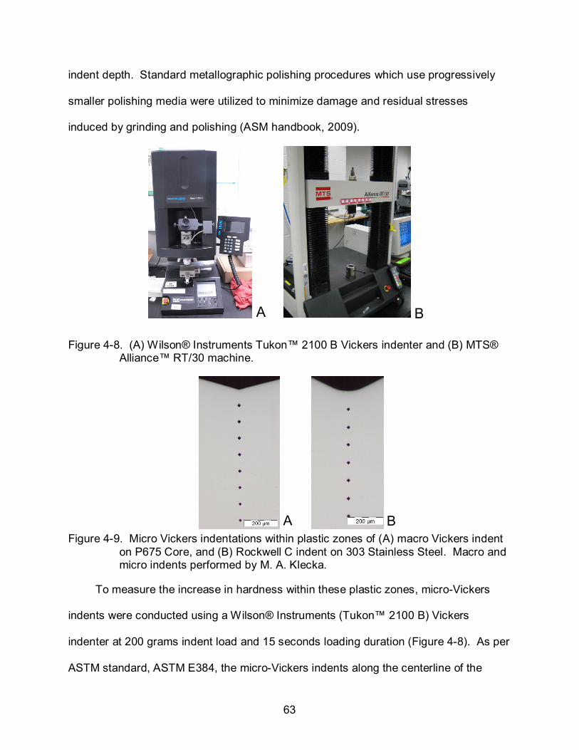
63
indent depth. Standard metallographic polishing procedures which use progressively
smaller polishing media were utilized to minimize damage and residual stresses
induced by grinding and polishing (ASM handbook, 2009).
A B
Figure 4-8. (A) Wilson® Instruments Tukon™ 2100 B Vickers indenter and (B) MTS® Alliance™ RT/30 machine.
A B Figure 4-9. Micro Vickers indentations within plastic zones of (A) macro Vickers indent
on P675 Core, and (B) Rockwell C indent on 303 Stainless Steel. Macro and micro indents performed by M. A. Klecka.
To measure the increase in hardness within these plastic zones, micro-Vickers
indents were conducted using a Wilson® Instruments (Tukon™ 2100 B) Vickers
indenter at 200 grams indent load and 15 seconds loading duration (Figure 4-8). As per
ASTM standard, ASTM E384, the micro-Vickers indents along the centerline of the

64
plastic zone were spaced 100 micrometers apart, as shown in Figure 4-9, to prevent
interaction with neighboring indents.
Figure 4-10. Plot of measured increase in Vickers hardness within plastic zone of (A)
Vickers macro indent of P675 and (B) Rockwell C indent of 303 stainless steel.
Figure 4-11. Flow curves taken from compression tests of (A) P675 and (B) 303 stainless steels. In-house compression tests performed by M. A. Klecka.
The resulting increase in hardness is shown in Figure 4-10 with respect to its virgin
state. Similar procedures of the micro-indentation of the plastic zone beneath a macro-
indent were also implemented by (Chaudhri, 1998; Srikant et al., 2006). Micro
indentations were performed along the plastic zone’s centerline because this
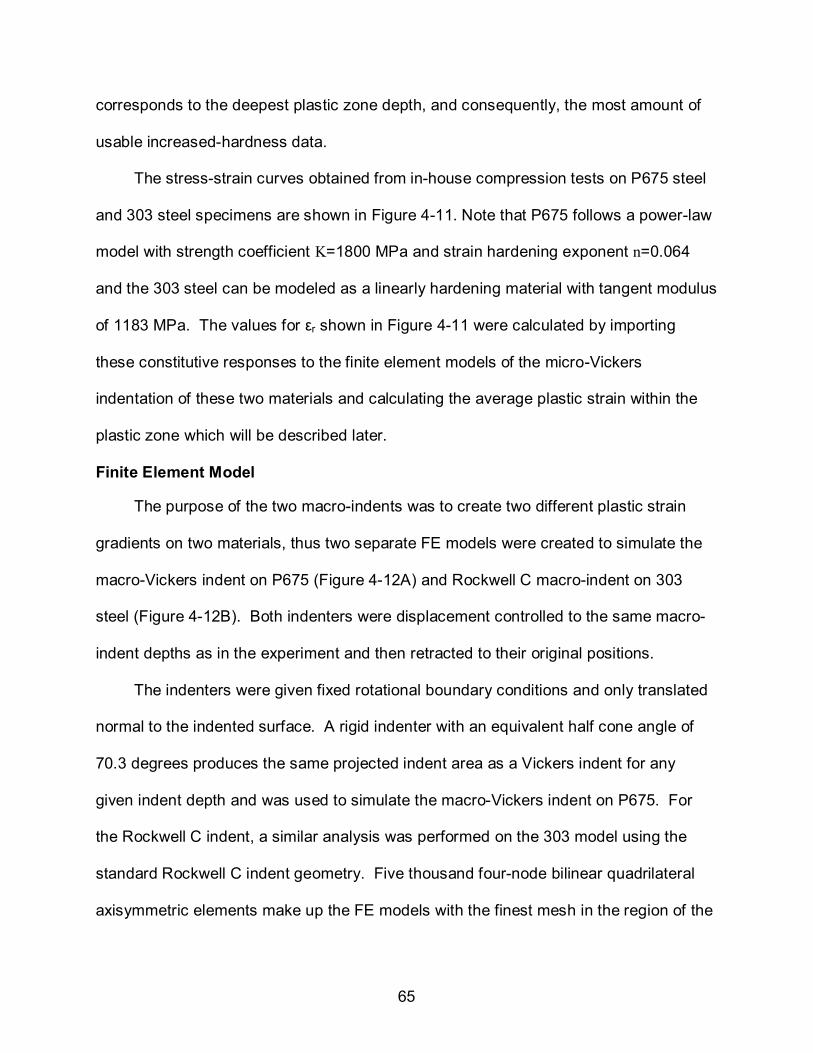
65
corresponds to the deepest plastic zone depth, and consequently, the most amount of
usable increased-hardness data.
The stress-strain curves obtained from in-house compression tests on P675 steel
and 303 steel specimens are shown in Figure 4-11. Note that P675 follows a power-law
model with strength coefficient K=1800 MPa and strain hardening exponent n=0.064
and the 303 steel can be modeled as a linearly hardening material with tangent modulus
of 1183 MPa. The values for εr shown in Figure 4-11 were calculated by importing
these constitutive responses to the finite element models of the micro-Vickers
indentation of these two materials and calculating the average plastic strain within the
plastic zone which will be described later.
Finite Element Model
The purpose of the two macro-indents was to create two different plastic strain
gradients on two materials, thus two separate FE models were created to simulate the
macro-Vickers indent on P675 (Figure 4-12A) and Rockwell C macro-indent on 303
steel (Figure 4-12B). Both indenters were displacement controlled to the same macro-
indent depths as in the experiment and then retracted to their original positions.
The indenters were given fixed rotational boundary conditions and only translated
normal to the indented surface. A rigid indenter with an equivalent half cone angle of
70.3 degrees produces the same projected indent area as a Vickers indent for any
given indent depth and was used to simulate the macro-Vickers indent on P675. For
the Rockwell C indent, a similar analysis was performed on the 303 model using the
standard Rockwell C indent geometry. Five thousand four-node bilinear quadrilateral
axisymmetric elements make up the FE models with the finest mesh in the region of the
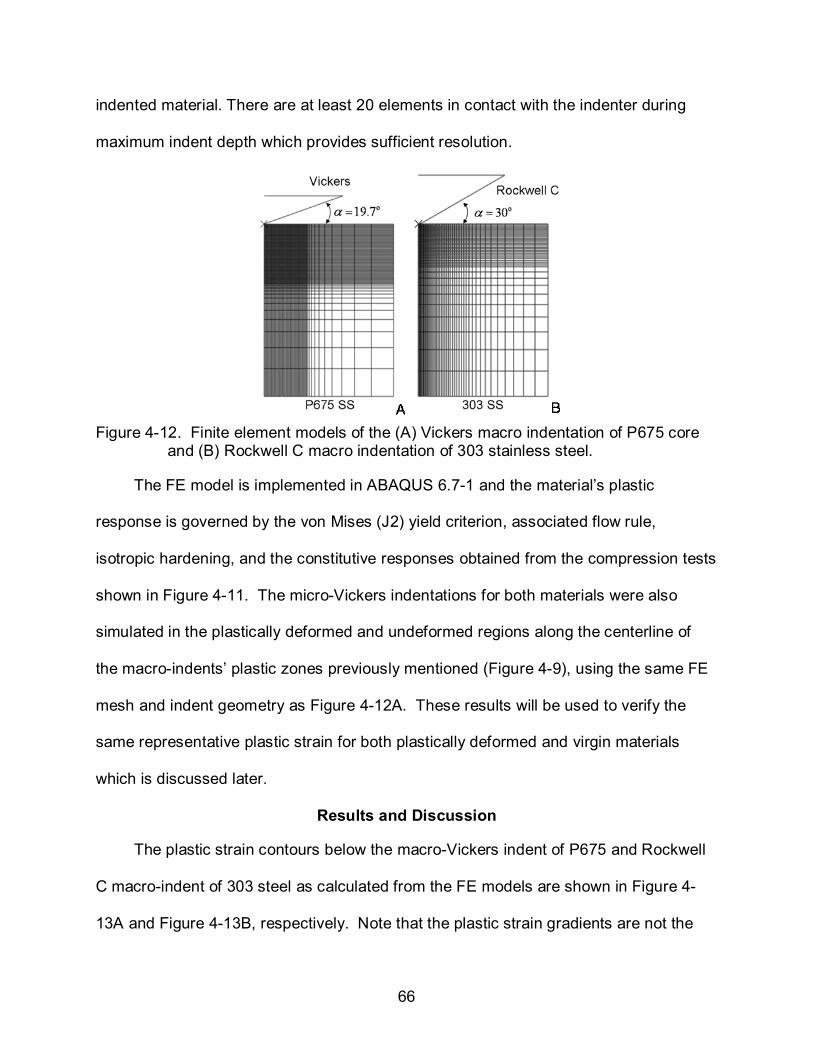
66
indented material. There are at least 20 elements in contact with the indenter during
maximum indent depth which provides sufficient resolution.
Figure 4-12. Finite element models of the (A) Vickers macro indentation of P675 core
and (B) Rockwell C macro indentation of 303 stainless steel.
The FE model is implemented in ABAQUS 6.7-1 and the material’s plastic
response is governed by the von Mises (J2) yield criterion, associated flow rule,
isotropic hardening, and the constitutive responses obtained from the compression tests
shown in Figure 4-11. The micro-Vickers indentations for both materials were also
simulated in the plastically deformed and undeformed regions along the centerline of
the macro-indents’ plastic zones previously mentioned (Figure 4-9), using the same FE
mesh and indent geometry as Figure 4-12A. These results will be used to verify the
same representative plastic strain for both plastically deformed and virgin materials
which is discussed later.
Results and Discussion
The plastic strain contours below the macro-Vickers indent of P675 and Rockwell
C macro-indent of 303 steel as calculated from the FE models are shown in Figure 4-
13A and Figure 4-13B, respectively. Note that the plastic strain gradients are not the
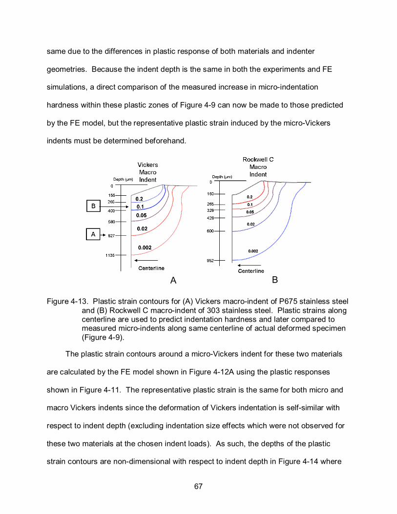
67
same due to the differences in plastic response of both materials and indenter
geometries. Because the indent depth is the same in both the experiments and FE
simulations, a direct comparison of the measured increase in micro-indentation
hardness within these plastic zones of Figure 4-9 can now be made to those predicted
by the FE model, but the representative plastic strain induced by the micro-Vickers
indents must be determined beforehand.
A B
Figure 4-13. Plastic strain contours for (A) Vickers macro-indent of P675 stainless steel and (B) Rockwell C macro-indent of 303 stainless steel. Plastic strains along centerline are used to predict indentation hardness and later compared to measured micro-indents along same centerline of actual deformed specimen (Figure 4-9).
The plastic strain contours around a micro-Vickers indent for these two materials
are calculated by the FE model shown in Figure 4-12A using the plastic responses
shown in Figure 4-11. The representative plastic strain is the same for both micro and
macro Vickers indents since the deformation of Vickers indentation is self-similar with
respect to indent depth (excluding indentation size effects which were not observed for
these two materials at the chosen indent loads). As such, the depths of the plastic
strain contours are non-dimensional with respect to indent depth in Figure 4-14 where
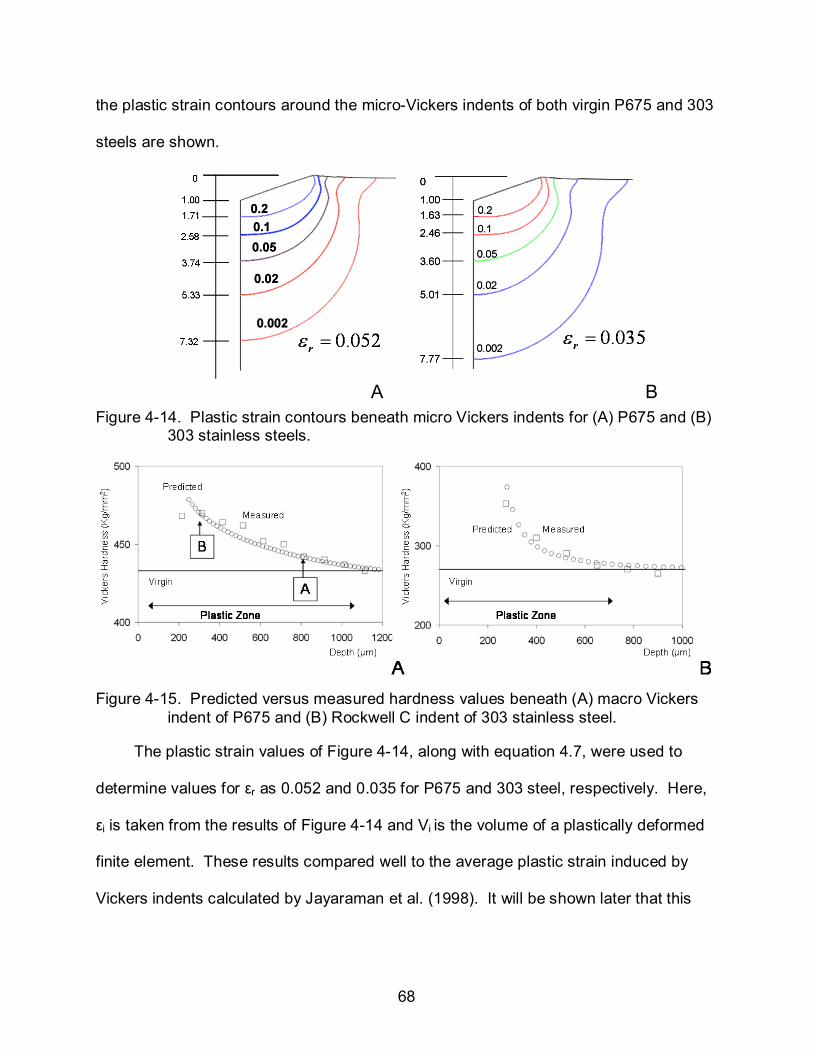
68
the plastic strain contours around the micro-Vickers indents of both virgin P675 and 303
steels are shown.
A B Figure 4-14. Plastic strain contours beneath micro Vickers indents for (A) P675 and (B)
303 stainless steels.
Figure 4-15. Predicted versus measured hardness values beneath (A) macro Vickers
indent of P675 and (B) Rockwell C indent of 303 stainless steel.
The plastic strain values of Figure 4-14, along with equation 4.7, were used to
determine values for εr as 0.052 and 0.035 for P675 and 303 steel, respectively. Here,
εi is taken from the results of Figure 4-14 and Vi is the volume of a plastically deformed
finite element. These results compared well to the average plastic strain induced by
Vickers indents calculated by Jayaraman et al. (1998). It will be shown later that this
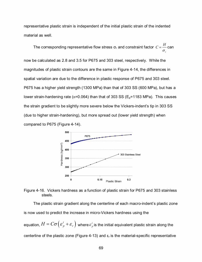
69
representative plastic strain is independent of the initial plastic strain of the indented
material as well.
The corresponding representative flow stress σr and constraint factor r
HCσ
= can
now be calculated as 2.8 and 3.5 for P675 and 303 steel, respectively. While the
magnitudes of plastic strain contours are the same in Figure 4-14, the differences in
spatial variation are due to the difference in plastic response of P675 and 303 steel.
P675 has a higher yield strength (1300 MPa) than that of 303 SS (600 MPa), but has a
lower strain-hardening rate (n=0.064) than that of 303 SS (Ep=1183 MPa). This causes
the strain gradient to be slightly more severe below the Vickers-indent’s tip in 303 SS
(due to higher strain-hardening), but more spread out (lower yield strength) when
compared to P675 (Figure 4-14).
Figure 4-16. Vickers hardness as a function of plastic strain for P675 and 303 stainless steels.
The plastic strain gradient along the centerline of each macro-indent’s plastic zone
is now used to predict the increase in micro-Vickers hardness using the
equation, ( )ip rH Cσ ε ε= + where i
pε is the initial equivalent plastic strain along the
centerline of the plastic zone (Figure 4-13) and εr is the material-specific representative
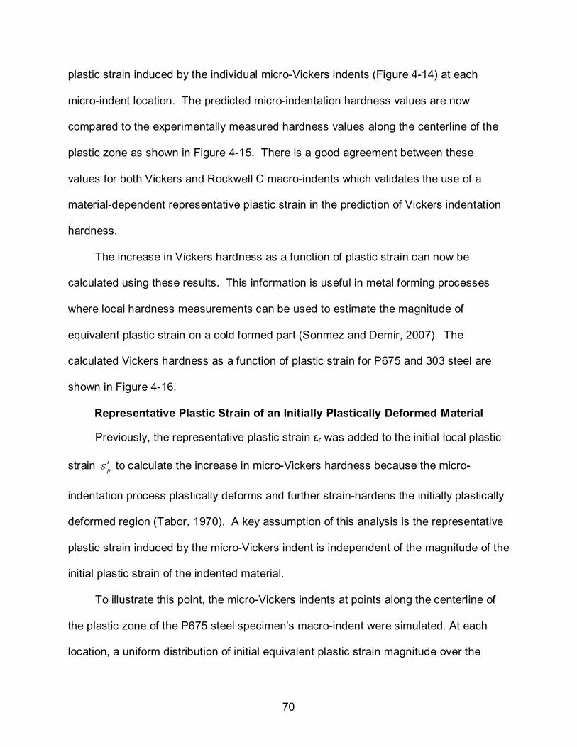
70
plastic strain induced by the individual micro-Vickers indents (Figure 4-14) at each
micro-indent location. The predicted micro-indentation hardness values are now
compared to the experimentally measured hardness values along the centerline of the
plastic zone as shown in Figure 4-15. There is a good agreement between these
values for both Vickers and Rockwell C macro-indents which validates the use of a
material-dependent representative plastic strain in the prediction of Vickers indentation
hardness.
The increase in Vickers hardness as a function of plastic strain can now be
calculated using these results. This information is useful in metal forming processes
where local hardness measurements can be used to estimate the magnitude of
equivalent plastic strain on a cold formed part (Sonmez and Demir, 2007). The
calculated Vickers hardness as a function of plastic strain for P675 and 303 steel are
shown in Figure 4-16.
Representative Plastic Strain of an Initially Plastically Deformed Material
Previously, the representative plastic strain εr was added to the initial local plastic
strain ipε to calculate the increase in micro-Vickers hardness because the micro-
indentation process plastically deforms and further strain-hardens the initially plastically
deformed region (Tabor, 1970). A key assumption of this analysis is the representative
plastic strain induced by the micro-Vickers indent is independent of the magnitude of the
initial plastic strain of the indented material.
To illustrate this point, the micro-Vickers indents at points along the centerline of
the plastic zone of the P675 steel specimen’s macro-indent were simulated. At each
location, a uniform distribution of initial equivalent plastic strain magnitude over the

71
small area of the micro-indent is assumed. The calculated equivalent plastic strain
magnitudes at locations A and B were 0.02 and 0.146 as illustrated in Figure 4-13A, and
the experimentally measured Vickers hardness values were 442 Hv and 470 Hv,
respectively (Figure 4-15A). The same FE mesh of Vickers indentation from Figure 4-
12A is used again for the simulations of the micro-Vickers indents of the pre-strained
points (A and B), except radial plastic strain magnitudes of 0.01 and 0.073 are now
applied to plastically strain-harden the material to the equivalent plastic strain states of
0.02 and 0.146, respectively, prior to indentation (Figure 4-17) as predicted by the
Cauchy’s strain-displacement equations for a cylindrical coordinate system.
A B
Figure 4-17. Schematic of the micro-Vickers indent of a pre-strained material: (A) region with same initial equivalent plastic strain throughout material prior to indentation and (B) illustration of additional plastic strain induced by the micro-indent.
The modified equation 4-7 is then written as( )i
j p jr
j
VV
ε εε
−= ∑
∑ where i
pε is the
initial equivalent plastic strain magnitude (0.02 or 0.146) of the indented material which
must be subtracted from the total equivalent plastic strain at every point within the new
plastic zone to determine the contribution of the additional plastic strain induced by the
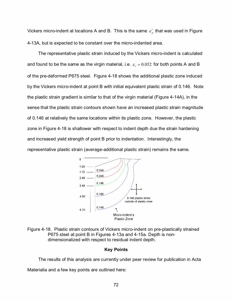
72
Vickers micro-indent at locations A and B. This is the same ipε that was used in Figure
4-13A, but is expected to be constant over the micro-indented area.
The representative plastic strain induced by the Vickers micro-indent is calculated
and found to be the same as the virgin material, i.e. 0.052rε = for both points A and B
of the pre-deformed P675 steel. Figure 4-18 shows the additional plastic zone induced
by the Vickers micro-indent at point B with initial equivalent plastic strain of 0.146. Note
the plastic strain gradient is similar to that of the virgin material (Figure 4-14A), in the
sense that the plastic strain contours shown have an increased plastic strain magnitude
of 0.146 at relatively the same locations within its plastic zone. However, the plastic
zone in Figure 4-18 is shallower with respect to indent depth due the strain hardening
and increased yield strength of point B prior to indentation. Interestingly, the
representative plastic strain (average-additional plastic strain) remains the same.
Figure 4-18. Plastic strain contours of Vickers micro-indent on pre-plastically strained P675 steel at point B in Figures 4-13a and 4-15a. Depth is non-dimensionalized with respect to residual indent depth.
Key Points
The results of this analysis are currently under peer review for publication in Acta
Materialia and a few key points are outlined here:

73
• This exercise demonstrates that the material-dependent volumetric average plastic strain induced by a Vickers indent is a valid representative plastic strain in the conversion of hardness to flow stress and independent of the initial plastic strain of an indented material.
• Vickers and Rockwell C macro-indentations were chosen in these experiments because they are relatively simple and inexpensive to produce and can create a controlled and convenient plastic strain gradients with plastic strains as high as 0.4. Such large plastic strains may otherwise be unobtainable in tension or compression tests or other modes of deformation. The large hydrostatic stresses and confinement associated with indentation prevent premature failure and make these high plastic strains possible. These plastic zones are relatively small in size which allows for multiple tests on a single specimen.
• Previous indentation methods do not examine the plastic zone to this detail nor has anyone verified the assumption that the representative strain is not a function of pre-plastic strain using finite element models of Vickers indentation with comparisons to experimental hardness data.
• This method predicts the increase in indentation hardness within the plastic zone of both Vickers and Rockwell C macro-indents and compared well to the experimentally measured micro-indent mapping for the plastic zones of 303 stainless steel and Pyrowear 675.
This method of relating indentation hardness to the plastic response for non-
graded materials using a material-dependent representative plastic strain will be used in
Chapters 5 and 6 to determine the plastic response of graded materials such as P675
and M50 NiL case-hardened bearing steels. These graded material properties are
needed to better understand spall propagation that occurs within the case layer of M50
NiL. If a material’s plastic response is proven to affect spall propagation, this
information can be used to design bearings with slower spall-propagation rates.

74
CHAPTER 5 INDENTATION OF GRADED MATERIALS
History of Graded Materials
The previous method in Chapter 4 was successful in determining relationships
between indentation hardness and material plastic response using a material-
dependent representative plastic strain; however methods to determine the plastic
response of graded materials are much more complicated. A plastically graded material
(PGM) is simply a substance that has a variation in plastic material response with depth
from its surface. It is possible that the plastic response of plastically-graded, case-
hardened M50 NiL bearing steel is affecting the spall propagation rate as shown in
Chapter 1. Graded materials are not unique to bearings and can be found throughout
the history of engineering as well as in nature.
Figure 5-1. Graded materials seen in nature (Grand Canyon) and in human-history (Japanese Katana)
Graded materials designed for a specific task have been around since the 1400’s.
The sharp cutting surface of the katana Japanese sword was made out of hard high-
carbon steel while the core of the sword consisted of a softer low-carbon steel to absorb
most of the impact and deformation. Special quenching techniques forced martensite to
form predominately on the cutting edge making it very hard and allowing it to retain its
sharpness with continued use (Figure 5-1).
75
Graded materials are also frequently seen in biology and nature. Tooth enamel is
hardest substance of the human body which reduces teeth wear from a lifetime of
chewing food and protects the softer dentine inner region of a tooth. Other bones in the
body have similar hard surfaces that protect the softer bone marrow within. The earth’s
surface is also graded and evidence can be seen in such places as the Grand Canyon.
The gradation from topsoil to bedrock influences the design of foundations for large
buildings. Graded materials that have soft surfaces and a progressively harder
subsurface are often used in impact-energy absorption applications. The soft surface
absorbs the energy from impact while the harder subsurface region maintains structural
shape and integrity. This is frequently seen in packaging by wrapping objects in bubble
wrap.
Graded materials with hard surfaces are desirable in mechanical components
such as gears and bearings where a hard and strong surface can withstand the large
contact stresses at the interface of contacting components while the ductile core
transmits the bulk of the shaft or thrust loads. Very hard surfaces are resistant to wear
and this greatly increases the rolling or sliding contact fatigue life of these components
which affects the overall health and performance of an engine.
Hardening the surfaces of these components is done in many different ways. The
most popular are carburizing, nitriding, or boriding, where carbon, nitrogen, or boron is
diffused into the surface of a part at relatively high temperature. These diffused atoms
are located at interstitial locations within the atomic lattice. This, along with special
quenching techniques, hinders plastic deformation and effectively makes the material
harder and stronger. The resulting variation in plastic response within a graded material
76
is difficult to determine by traditional methods such as compression or tension tests due
to the interactions of the stronger and weaker regions and complications in fabricating a
test specimen with the same composition as a given point within the graded region.
Despite these difficulties, the variation in material properties are needed to design
stronger and longer lasting mechanical parts. Understanding how diffusion and heat
treatment affect the plastic response is crucial. There are many different ways to
estimate material properties; one of the simpler and easier methods is through
indentation analysis.
Previous Methods to Determine Plastic Response of PGMs
Instrumented indentation of graded materials is a relatively new area of research.
Nakamura et al. (2000) used instrumented ball indentation and Kalman filtering
techniques to estimate the variation in plastic response of PGMs. They used a standard
rule of mixtures to determine the stress and strain contributions from the metal and
ceramic portions of the PGM. The variation in ceramic phase fraction resulted in a
change in plastic response with depth. The plastic responses of both ceramic and
metal phases must be known a priori. A set of PGM indentation reference behavior was
created by many FE model simulations and experimental verification of this method was
done by Gu et al. (2003).
Giannakopoulos (2002) used analytical and numerical methods to analyze the
deformation induced by sharp indentation of PGMs, but this was limited to nonlinear
elastic and perfectly plastic materials. Nayebi et al. (2002) predicted the decreasing
hardness profile of nitrided steels using instrumented ball indentation and finite element
analysis.

77
Cao and Lu (2004) used finite element analysis to simulate conical indentation of
PGMs and the resulting load displacement curves were used in a reverse analysis to
predict its plastic response. Their analysis used the method of Dao et al. (2001) to
determine a set of dimensionless functions that describe the indentation behavior of
PGMs for various gradients in yield strength only. The resulting indentation loading
curvature (Cv) can vary with indentation depth (d) for a PGM and reflects the degree of
gradation in subsurface yield strength.
Choi et al. (2008) showed how the yield strength gradient of a PGM affects
indentation loading curvature, distribution of maximum principal and von Mises stresses,
and equivalent plastic strain gradient within the plastic zone of a conical indent. They
used dimensionless functions that describe the indentation loading curvatures taken
from homogeneous elastic materials (Johnson, 1987) and non-graded elasto-plastic
materials (Dao et al., 2001) to create a new dimensionless function that describes the
indentation loading curvature of PGMs. Experimental validation was done by Choi et al.
(2008) on graded materials created by electro-deposition techniques which created a
variation in grain size and consequently yield strength.
The above mentioned PGM indentation methods relied heavily upon instrumented
sharp or ball indentation. These devices are expensive, hard to calibrate
(VanLandingham, 2003), and may not be available at some research labs or
universities. Also, two different strain hardening materials can produce the same
indentation loading curvature in single indenter methodologies (Chollacoop et al., 2003).
Most of the previous methods assumed only a variation in yield strength with no
change in parameters such as strain hardening exponent. Some of these methods
78
analyzed materials that were created in labs by electro-deposition or thermal-spraying
by plasma guns. However, these are not good examples of engineering materials that
are needed to survive the harsh environments frequently experienced in jet engine
bearings. These methods investigated how the variations in plastic response affected
the indentation loading curvature of PGMs. Very few of these methods investigated the
actual plastic deformation induced by the indentation of PGMs. In just about all of the
methods the material properties of the surface or substrate were required to estimate
the material properties of neighboring graded material. These methods needed many
FE model simulations and used complex algorithms such as Kalman filtering techniques
or curve fitting dimensionless functions to encompass the indentation behavior of a
given range of material properties. Ogasawara et al. (2007) has shown that some of
these ranges of material properties may not be broad enough to encompass all
engineering materials.
Proposed Method
The method presented here will use macro and micro Vickers indentation and
elastic-plastic finite element analysis (FEA) to determine the variation in constitutive
response of the plastically graded, case hardened region of Pyrowear 675 (P675)
stainless steel which is frequently used in current high-performance aerospace bearings
and gears. The PGM utilized here has a variation in plastic response with depth, but
constant elastic modulus. The fact that a strain hardening material exhibits an increase
in hardness due to plastic deformation compared to its virgin hardness is utilized here in
both the measurement and prediction of Vickers hardness for a relatively large
magnitude and range of plastic strain within this PGM.

79
A convenient and controlled way to induce large magnitudes of plastic strain within
a PGM is via macro-Vickers indentation which induces a plastic strain gradient
throughout its plastic zone (Figure 5-1) that is symmetric about its centerline. Within
this region of plastic deformation, the material will strain harden according to its plastic
response and consequently display an increase in indentation hardness with respect to
its virgin state.
The principal concept of this analysis is that the increase in hardness (converted to
flow stress using the analysis of Chapter 4) at a given depth with respect to its virgin
state must fall on the flow curve defined at that depth as depicted in Figure 5-1. The
increase in hardness within the plastic zone is experimentally measured by micro-
Vickers indentations which are then compared to those predicted by finite element
models described later. The micro-indents (≈ 200g indent load) essentially probe the
increased yield strength within the plastic zone of the macro-indent (>150Kg). The
increase in yield strength can be predicted by finite element modeling provided the
appropriate flow curves are used at every point throughout the PGM. The increased
yield strength will correspond to a certain amount of plastic strain which is dependent on
the strain hardening characteristics of the flow curves which vary with depth.
As an example, for a PGM with decreasing hardness with depth (Figure 5-1) the
yield strength is also expected to decrease since hardness is indicative of yield strength
(Tabor, 1970). Thus the micro-hardness values at a specific depth from the surface and
within the plastic zone will provide the increased flow stresses that must fall on the flow
curve at that depth. Outside of the plastic zone, any hardness measurements will
reflect the virgin (undeformed) initial yield strength at that depth.

80
For instance, the hardness measurement at location n in Figure 5-1 will probe the
yield strength of a virgin region because it is outside of the plastic zone caused by the
macro-indent. The hardness measurements along Row a are expected to be greater
than the hardness at n due to the strain-hardening within the plastic zone, while keeping
in mind that the flow stresses for any material point along Row a must fall on the same
flow curve as point n.
Hardness converted to flow stress
pε
σ
H Cσ=mσ
1σ2σ
nσ
0pε =
Same Plastic Response
Gradient in Plastic
Response
Gradient in plastic
strain Micro
Vickers Indents
Macro-Indent
1 2 m
1 2 n
Plastic Zone
Boundary 0pε =
….
….1σ
2σRow a
Row b
Figure 5-1. Schematic of the relationship between indentation hardness and plastic response at any given depth within the plastic zone of a PGM.
The same holds true for Row b and point m, but the magnitudes would be lower
due to the decreasing-hardness trend in this PGM example. This information, along
with the corresponding plastic strain obtained from FE models, will be utilized to
determine the variation in plastic response with depth for this commercially available,
case hardened P675 stainless steel by using the relationship between Vickers hardness
and yield strength described in Chapter 4, namely ( )r pH Cσ ε ε= + where εp is the initial
plastic strain within the macro indent’s plastic zone, εr is the representative plastic strain
induced by the micro-indentation process, and C is the constraint factor. All of these
terms will vary with depth for a plastically deformed, graded material.

81
Material
Prior to carburization and heat treatment, the P675 steel contains only 0.07%
carbon. After carburization, the surface of the case-hardened layer can contain up to
1% carbon which decreases with depth due to the carbon diffusion process. Additional
heat treatment involving double-tempering is used to lock in the final microstructure of 2
µm in size which consists of tempered martensite and dispersed carbide particles. The
variation of carbide particle volume fraction with depth results in a variation in hardness
and plastic response over the case hardened region. Note the high Chromium content
for this stainless steel in Table 5-1.
Table 5-1. Material composition of P675 Stainless Steel (Carpenter, 2009).
To determine the variation in virgin hardness with depth within this specific PGM,
the samples were sectioned, ground, and polished on surfaces parallel to the carbon
gradient. Standard metallographic polishing procedures which use progressively finer
polishing media were used to minimize damage and residual stresses induced by
polishing (ASM Handbook, 2009). Micro Vickers-indentations were conducted on this
cross-section using a Wilson® Instruments (Tukon ™ 2100B) Vickers indenter (Figure
5-4A) at 200g, 500g, and 1Kg indent loads for 15 seconds loading duration. The
indents were spaced 2.5 times the indent diagonal to prevent interactions with
neighboring indents as per ASTM E384 standard.
The Vickers hardness versus depth profile shown in Figure 5-2 for the virgin P675
steel depicts negligible indentation size effect (ISE) for this chosen indent load range.
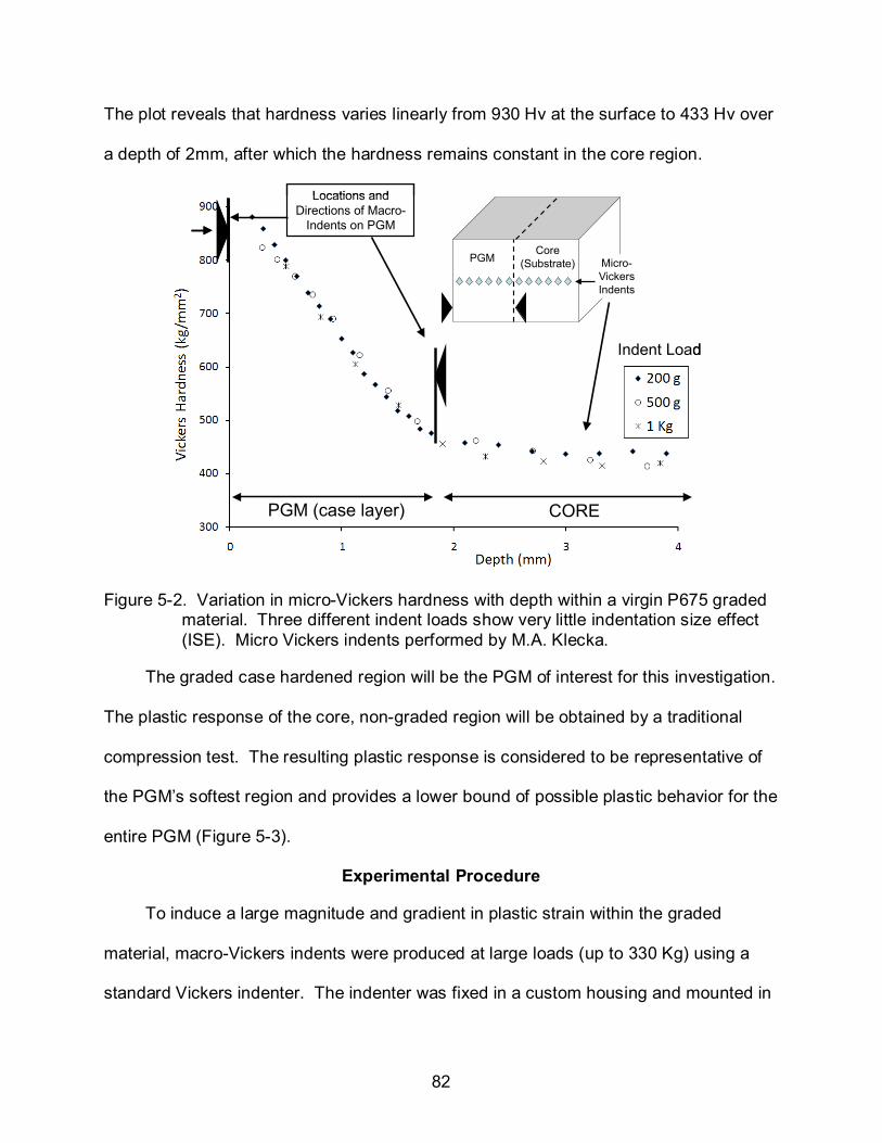
82
The plot reveals that hardness varies linearly from 930 Hv at the surface to 433 Hv over
a depth of 2mm, after which the hardness remains constant in the core region.
PGM (case layer) CORE
Locations and Directions of Macro-
Indents on PGM
Indent Load
PGMCore
(Substrate) Micro-Vickers Indents
PGM (case layer) CORE
Locations and Directions of Macro-
Indents on PGM
Indent Load
PGMCore
(Substrate) Micro-Vickers Indents
Figure 5-2. Variation in micro-Vickers hardness with depth within a virgin P675 graded material. Three different indent loads show very little indentation size effect (ISE). Micro Vickers indents performed by M.A. Klecka.
The graded case hardened region will be the PGM of interest for this investigation.
The plastic response of the core, non-graded region will be obtained by a traditional
compression test. The resulting plastic response is considered to be representative of
the PGM’s softest region and provides a lower bound of possible plastic behavior for the
entire PGM (Figure 5-3).
Experimental Procedure
To induce a large magnitude and gradient in plastic strain within the graded
material, macro-Vickers indents were produced at large loads (up to 330 Kg) using a
standard Vickers indenter. The indenter was fixed in a custom housing and mounted in
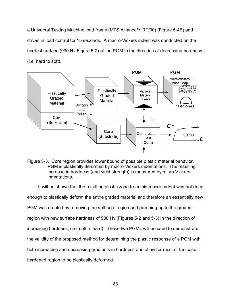
83
a Universal Testing Machine load frame (MTS Alliance™ RT/30) (Figure 5-4B) and
driven in load control for 15 seconds. A macro-Vickers indent was conducted on the
hardest surface (930 Hv Figure 5-2) of the PGM in the direction of decreasing hardness,
(i.e. hard to soft).
Figure 5-3. Core region provides lower bound of possible plastic material behavior. PGM is plastically deformed by macro-Vickers indentations. The resulting increase in hardness (and yield strength) is measured by micro-Vickers indentations.
It will be shown that the resulting plastic zone from this macro-indent was not deep
enough to plastically deform the entire graded material and therefore an essentially new
PGM was created by removing the soft core region and polishing up to the graded
region with new surface hardness of 500 Hv (Figures 5-2 and 5-3) in the direction of
increasing hardness, (i.e. soft to hard). These two PGMs will be used to demonstrate
the validity of the proposed method for determining the plastic response of a PGM with
both increasing and decreasing gradients in hardness and allow for most of the case
hardened region to be plastically deformed.

84
The macro-Vickers indents (Figure 5-2) were sectioned and polished up to the
indent diagonals (Figure 5-5) which correspond to the maximum indent and plastic zone
depths. Standard metallographic polishing procedures were used to prevent residual
stress accumulation and additional plastic deformation induced by polishing (ASM
Handbook, 2009). Micro-Vickers indents were then conducted on these cross-sections
at 200 grams indent load and 100 µm spacing to measure the increase in hardness
within the plastic zone of the macro-Vickers indent. The micro-Vickers indents of the
cross sections of the hardest and softest macro-indents are shown in Figure 5-5A and
5-5B, respectively.
A B
Figure 5-4. (A) Wilson® Instruments Tukon™ 2100 B Vickers indenter and (B) MTS® Alliance™ RT/30 machine.
The variation in hardness can be seen visually in Figure 5-5 where the micro-
indent sizes change along the cross-section. Because the indent load is the same for
all micro-indents, the hardest regions have smaller indent sizes when compared to the
softest regions. This method of micro-indent mapping below a macro indent is similar to
the approaches adopted by (Koeppel et al., 1999; Srikant et al., 2006; Chaudhri, 1998),
but will be extended here to predict the variation in flow curves of a PGM.

85
The macro-Vickers indentation on the hardest PGM surface (Figure 5-5A) was
created by an indent load of 330 Kg which resulted in an average diagonal length of 800
µm. The increase in micro-Vickers hardness along the centerline of the plastic zone is
depicted in Figure 5-6A. The maximum increase in hardness is approximately 50 Hv in
the region of highest plastic strain and it decreases to the virgin hardness value at the
plastic zone boundary.
Soft 500Hv
Hard
Macro-Indent 230 Kg
Macro-Indent 330 Kg
Micro Vickers Indents
Micro Vickers Indents
Hard930 Hv
Soft
A B Figure 5-5. Micro-Vickers indent (200 g) map within plastic zone induced by the macro-
Vickers indention on (A) the hardest and (B) softest surfaces of the PGMs. Notice smaller micro-indent sizes within the hardest region. Macro and micro Vickers indents performed by M.A. Klecka.
If this region had a perfectly plastic response with depth, there would have been
no strain hardening, no increase in flow stress, and consequently no increase in
hardness within the plastic zone of the macro-indent. Thus the increase in hardness
within the plastic zone is dependent on material strain hardening properties and the
magnitude of plastic strain. The increase in hardness along the centerlines of the
macro-indent’s plastic zones is shown because this region has the deepest plastic zone
depth which includes the gradient in plastic response. Also, the hardness

86
measurements along the centerline correspond to the highest plastic strain (and flow
stress) experienced at any specific depth from the surface.
Figure 5-6. Experimentally measured micro-Vickers hardness along the centerline of
the macro indent for (A) hardest and (B) softest PGMs. Micro Vickers indents performed by M.A. Klecka.
A similar procedure was conducted on the softest PGM surface that has an
increasing subsurface hardness trend with depth (Figure 5-5B). The macro-indent on
the softest surface (500 Hv) was conducted at a reduced load of 230 Kg but resulted in
a larger indent diagonal of 940µm. Similarly, the increase in hardness along the
centerline of the plastic zone is shown in Figure 5-6B. The maximum increase in
hardness is again approximately 50 Hv in the region of large plastic strain and
decreases to zero at the elastic-plastic boundary.
The increase in hardness within the plastic zones of both PGMs is indicative of the
material’s ability to strain-harden. The question yet to be answered, however, is what
equivalent plastic strain magnitude corresponds to the above measured hardness (flow
stress) values? To answer this question, these macro-Vickers indentation experiments
of graded materials are simulated in finite element models. The flow curve variation
with depth will be estimated from the flow curve of the core region and the variation in

87
hardness with depth within the PGM. The measured increase in micro hardness within
the plastic zone of the macro-indent will be estimated from the equivalent plastic strain
calculated by the FE model.
Constitutive Response
Determining the constitutive response of any given point within the PGM using
traditional methods such as a tension and compression test is impractical because of
the difficulty in preparing a specimen of uniform composition that corresponds to any
given point within the PGM. However, the core region has uniform microstructure and
hardness (Figure 5-2), and the ample amount of core material available allows for a
compression test specimen of 10 mm x 6 mm x 3.175 mm to be extracted.
Figure 5-7. (A) MTS load frame is used to determine (B) flow curve obtained from
compression test of the homogeneous core. Compression test performed by M.A. Klecka.
The compression test was conducted in a MTS load frame (Figure 5-7A). The
power-law curve fit, nKσ ε= , applied to the flow curve obtained from this compression
test shown in Figure 5-7B resulted in a strength coefficient K = 1800 MPa and a strain
hardening exponent n = 0.064. Because this is the softest region of the PGM, this
information provides a lower bound of possible plastic behavior for the entire PGM.
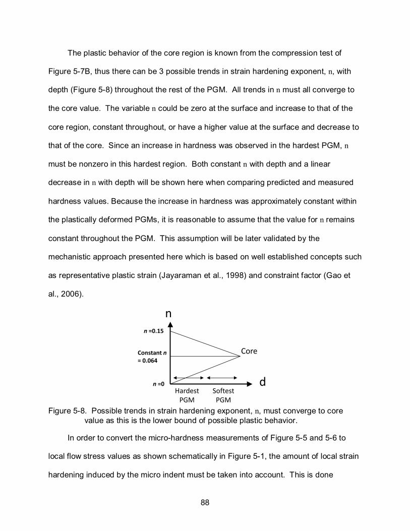
88
The plastic behavior of the core region is known from the compression test of
Figure 5-7B, thus there can be 3 possible trends in strain hardening exponent, n, with
depth (Figure 5-8) throughout the rest of the PGM. All trends in n must all converge to
the core value. The variable n could be zero at the surface and increase to that of the
core region, constant throughout, or have a higher value at the surface and decrease to
that of the core. Since an increase in hardness was observed in the hardest PGM, n
must be nonzero in this hardest region. Both constant n with depth and a linear
decrease in n with depth will be shown here when comparing predicted and measured
hardness values. Because the increase in hardness was approximately constant within
the plastically deformed PGMs, it is reasonable to assume that the value for n remains
constant throughout the PGM. This assumption will be later validated by the
mechanistic approach presented here which is based on well established concepts such
as representative plastic strain (Jayaraman et al., 1998) and constraint factor (Gao et
al., 2006).
Figure 5-8. Possible trends in strain hardening exponent, n, must converge to core
value as this is the lower bound of possible plastic behavior.
In order to convert the micro-hardness measurements of Figure 5-5 and 5-6 to
local flow stress values as shown schematically in Figure 5-1, the amount of local strain
hardening induced by the micro indent must be taken into account. This is done
n
d
Core
Hardest PGM
Softest PGM
Constant n= 0.064
n =0
n =0.15

89
through the concept of representative plastic strain, εr, which is a measure of the
average or “representative” plastic strain induced by a Vickers indent and discussed in
more detail in Chapter 4. The representative plastic strain describes the extent that the
average flow stress within the plastic zone exceeds the initial yield strength of the
indented material.
A B
Figure 5-9. (A) Expanding cavity model for strain hardening materials assumes hemispherical deformation below tip of indent. (B) Resulting relationship between H/σy and E/σy. (Gao et al., 2006).
Calculated values for this average or representative plastic strain as a function of n
can be found in (Jayaraman et al., 1998) and will not be repeated here. For n = 0.064 of
the core region, 0.052rε = and its corresponding representative flow stress is 1506 MPa
which has a constraint factor given by 2.82( )r
HCσ ε
= = . Recall that εr is a function of n
only (Jayaraman et al., 1998), and therefore the value for representative plastic strain is
also constant regardless of the location within the PGM because n is assumed to be
constant throughout. The flow stress at the corresponding representative plastic strain

90
defines one point on the material flow curve, ( )rHC
σ ε = provided the values of C and H
(Figure 5-2) are known a priori.
The relationship between hardness, yield strength, elastic modulus, and strain
hardening exponent for power-law hardening materials was derived by Gao et al. (2006)
using expanding cavity models in the following form:
12 1 3 1 cot1 33 4
n
yy
EHn n
ασσ
= +− +
(5.1)
where α is the equivalent half cone angle for Vickers indenters and has a value of 70.3
degrees. A visual representation of the dependence of y
Hσ
on y
Eσ
from this expanding
cavity model is shown in Figure 5-9b. Note for low values of n, y
Hσ
is approximately 3
which agrees with the predictions of Tabor (1970). The expanding cavity models of
(Johnson, 1970; Hirst and Howse, 1969; Marsh, 1964) are based on the solution by Hill
(1950) for the quasi-static expansion of an internally pressurized spherical shell of
perfectly plastic materials (Gao et al., 2006).
The expanding cavity model assumes that the deformation beneath Vickers
indentation is hemispherical in nature and the plastic deformation is caused by a small
“core” of large hydrostatic stress beneath the tip of the indent as shown in Figure 5-9A.
For strain hardening materials, the stress-displacement equations for an internally
pressurized spherical shell were derived by Gao and Wei (1991) and extended by Gao
et al. (2006) to create the ECM used in this analysis. For indentation, the hardness of
the material is taken to be the mean pressure acting on the interface between the

91
hydrostatic core and the plastic zone and compares well to the hardness predicted by
experiments and finite element analysis Gao et al. (2006).
Strength Coefficient, K (MPa)
Yield Strength, σy (MPa)
σy
Strength Coefficient, K (MPa)
Yield Strength, σy (MPa)
σy
Figure 5-10. Strength coefficient K and Yield strength as function of depth.
Figure 5-11. (A) Power -law flow curves as function of hardness and (B) ratio of hardness to flow stress at the corresponding representative plastic strain.
Because H and n are known for all depths, and assuming that E=200 GPa for
steel, the yield strength σy can then be determined from the above relationship for the
entire PGM from this equation and shown in Figure 5-10. The strength coefficient K as
function of hardness (H) taken can now be calculated 1n nyK E σ −= from the intersection
of the elastic y yEσ ε= and plastic ny yKσ ε= stress-strain curves which vary with depth
92
for a PGM. The resulting flow curves as a function of hardness is shown in Figure 5-
11A. The constraint factor ( )r
HCσ ε
= can now be calculated and shown in Figure 5-
11B. This data will be used to predict the Vickers hardness for a plastically deformed
PGM using the equivalent plastic strain calculated by FE models described in the
following section.
Finite Element Model
To determine if these flow curves accurately represent the plastic behavior of the
PGM, the plastic strain induced by the macro-indent must be determined and then
related to the micro-Vickers hardness measurements discussed earlier. The plastic
strain is dependent on the material’s ability to resist plastic deformation, i.e. its strain
hardening characteristics and yield strength. Determination of the plastic strain
magnitude and gradient with depth beneath a Vickers indent is difficult, particularly for a
PGM, thus finite element modeling provides a convenient way to compute the plastic
strain gradient beneath these macro-indents.
In this axisymmetric model, a rigid conical indenter with a half cone angle of 70.3
degrees produces the same indentation area as a Vickers indent for any given indent
depth and does not require a mesh (Figure 5-12). The indenter is displacement
controlled to the same depth as in the experiment and then retracted to its original
position. The indenter is given fixed rotational boundary conditions and allowed to
translate normal to the specimen surface. Four thousand eight hundred four-node
bilinear quadrilateral axisymmetric elements make up the Finite Element (FE) model
with the finest mesh in the region closest to the indenter tip. The FE model is
implemented in ABAQUS 6.7-1. The plastic response is governed by the von Mises

93
(J2) yield criterion, associated flow rule, and isotropic hardening. The flow curve
variation of Figure 5-11A is inserted into the finite element model and the macro-
indentations of both hardest (Figure 5-5A) and softest (Figure 5-5B) PGMs are
simulated to the same macro-indentation depths as the experiments.
ε
σ Hard
Soft
o19.7α =
PGM
CORE
Figure 5-12. FE model of the macro-Vickers indentation of a PGM.
Results
The contours of constant equivalent plastic strain within the plastic zones as
calculated by the FE models of both PGMs are shown in Figure 5-13A. Note that the
indentation on the hardest PGM surface has a shallower macro-indent depth (d=118 µm
at 330Kg indent load) than the deeper macro-indent and lower indent load (230 Kg) on
the softest PGM surface (d=130 µm). However, the plastic zone for the hardest PGM is
deeper and narrower than the plastic zone of the softest PGM. The surface of the
hardest PGM is more resistant to plastic deformation and therefore forces plastic
deformation to occur within the weaker, subsurface region.
Although the softest PGM surface has a deeper macro-indent, it has a shallower
and wider plastic zone because the softest-surface region accommodates most of the
plastic deformation while the subsurface regions are harder and more resistant to
plastic deformation. These results show that distribution of plastic strain is sensitive to

94
the gradation in plastic response. The equivalent plastic strains along the centerlines of
both PGMs increase asymptotically as shown in Figure 5-13B. This information will be
used to predict the micro-Vickers hardness measurements of Figure 5-6.
Figure 5-13. (A) Equivalent plastic strain contours within the plastic zones induced by Vickers macro-indents on hardest and softest surfaces of the PGMs. (B) Comparison of the plastic strain magnitudes along centerlines of both PGMs as measured from material surface.
The predicted micro-Vickers hardness at a given location j at any depth within the
PGM plastic zone can now be determined by the equation: ( )r pH Cσ ε ε= + where jpε is
the initial plastic strain induced by the macro-Vickers indent (Figures 5-13A and 5-13B)
and jrε is the representative plastic strain induced by the micro-Vickers indent at a given
location. For the case where n is a constant 0.064 with depth, 0.052jrε = is constant
with depth also. The flow stress that corresponds to the sum total of the representative
plastic strain and equivalent plastic strain is calculated for every point within the plastic
zone and then multiplied by C to predict the micro-Vickers hardness values. These
hardness values are then compared to the experimentally measured hardness in Figure
5-6 and shown again in Figure 5-14. Good agreement is seen between the predicted
and measured hardness values along the centerlines of both macro indents. The
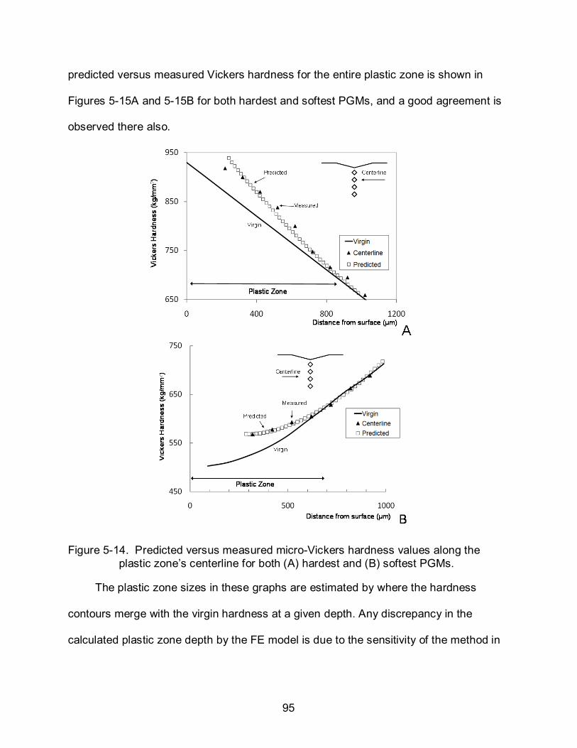
95
predicted versus measured Vickers hardness for the entire plastic zone is shown in
Figures 5-15A and 5-15B for both hardest and softest PGMs, and a good agreement is
observed there also.
Figure 5-14. Predicted versus measured micro-Vickers hardness values along the plastic zone’s centerline for both (A) hardest and (B) softest PGMs.
The plastic zone sizes in these graphs are estimated by where the hardness
contours merge with the virgin hardness at a given depth. Any discrepancy in the
calculated plastic zone depth by the FE model is due to the sensitivity of the method in

96
predicting hardness at low plastic strain, experimental scatter in measured hardness,
and the fact that the plastic zone boundary is defined at the 0.002 plastic strain contour.
Plastic Zone
Contours of Constant Hardness
Distance away from centerline (µm)
Y, d
epth
from
sur
face
(µm
)
Predicted Hardness Measured Hardness
Plastic Zone
Contours of Constant Hardness
Distance away from centerline (µm)
Y, d
epth
from
sur
face
(µm
)Predicted Hardness Measured Hardness
(a)
Hard
Soft
Soft
Hard
A
B
Figure 5-15. Predicted versus measured micro-Vickers hardness values for the (A) hardest and (B) softest PGMs within the entire plastic zone of the macro-Vickers indentations.
The predicted hardness is expected to have an increasing trend as it approaches
the indenter tip because the flow stresses of the power-law plastic response increase
with increasing plastic strain and the plastic strain asymptotically increases close to the

97
indenter tip as observed in Figure 5-13B. Note that there is good agreement between
the measured and predicted hardness values for both PGMs irrespective of the
increasing or decreasing hardness gradients below the surface. This validates the
assumption of constant strain hardening exponent with depth for this specific case-
hardened stainless steel.
Since the graded layer gradually merges with the core material, the assumption of
constant strain hardening exponent for the PGM is logical. It will be shown next that a
different set of flow curves predicts different micro-Vickers hardness values within the
plastic zone of the macro-Vickers indent for the same macro-indent depths. Although
the PGM used in this analysis has a constant strain hardening exponent, this method
can be applied to PGMs that have variations in n as well because the expanding cavity
model derived by Gao et al. (2006) takes into account the dependence of hardness on
n. This will be seen in Chapter 6 where the variation in plastic response is determined
for case hardened M50 NiL, where the flow curve of the core region is initially unknown.
Variation in Strain Hardening Exponent
To show an example of how a different variation in plastic response can predict
different hardness values, a new trend in strain hardening exponent is created and a
new set of material properties will be inserted into the same FE indentation-models as
before. The new strain hardening exponent at the hardest surface of the PGM will be
assumed as n = 0.15 and will decrease linearly to the core where n = 0.064 (Figures 5-8
and 5-16). Once again, the strain hardening exponent of the core cannot be changed
because it was determined from the compression test of the core region. The
representative plastic strain rε is dependent only on the strain hardening exponent so

98
rε is now 0.035 at the hardest region where n = 0.15 and increases linearly to 0.052 for
n = 0.064 at the softest region (Figure 5-17). To find ( )r nε one may refer to the
calculations by Jayaraman et al. (1998) or calculate individually for each n value through
FE simulations of the Vickers indentation process shown in Chapter 4. S
train
Har
deni
ng E
xpon
ent,
n
Depth (µm)
Stra
in H
arde
ning
Exp
onen
t, n
Depth (µm) Figure 5-16. New trend in strain hardening exponent (n) is created to determine how
material properties affect predicted hardness values.
The yield strength and strength coefficient K are determined as before using the
expanding cavity model of Gao et al. (2006) and shown in Figure 5-18A. The new set of
flow curves as a function of hardness is shown in Figure 5-18B. Note that the virgin
hardness trend is unchanged and this new variation in flow curves still yields the same
virgin hardness as the constant-n trend used before. However, for a given amount of
plastic deformation the increase in hardness will not be the same for different strain
hardening materials.
The core material’s strain hardening exponent cannot be changed which means
the new set of material properties will not deviate much from the initial set (constant-n)
in this softest region. Therefore, the softest PGM FE model does not need to be
simulated again. These new flow curves are inserted into the indentation-FE model of

99
the hardest region of the PGM because this is where the greatest deviation from the
initial set of material properties occurs.
Strain Hardening Exponent, n
Rep
rese
ntat
ive
Pla
stic
Stra
in, ε
r
Strain Hardening Exponent, n
Rep
rese
ntat
ive
Pla
stic
Stra
in, ε
r
Figure 5-17. Representative plastic strain as function of strain hardening exponent, n.
Calculations can be found in (Jayaraman et al., 1998) and Chapter 4.
Figure 5-18. (A) New trends in σy, K, and n allow for (B) new flow curves to be created
as function of hardness (depth of PGM). Note material properties of core material cannot change because K and n of core were determined by compression test and provide lower bound of possible plastic behavior.
The macro-indent of the hardest PGM is simulated again with the new material
properties to the same depth as before and the equivalent plastic strain gradient is
calculated by the FE model. The depth-dependent representative strain is added to the
equivalent plastic strain at every point of interest and then converted to predicted-
hardness values while taking into account the variation in both K and n using the same
relationship between indentation hardness and flow stress, ( )r pH Cσ ε ε= + . The new

100
predicted hardness values are plotted against the measured hardness from Figure 5-14
and shown again in Figure 5-19. As shown, the new predicted hardness values do not
match the experimentally measured ones when the strain hardening exponent of the
hardest region is effectively doubled as compared to the initial test case. For
completeness, the virgin hardness as predicted by the same equation ( )r pH Cσ ε ε= +
when 0pε → [i.e. ( )rH Cσ ε= ] also displays a good match to the virgin hardness trend,
thus verifying that these flow curves still predict the same virgin hardness.
Plastic Zone
Distance from surface (µm)
Vic
kers
Har
dnes
s (k
g/m
m2 )
Centerline
( )rH Cσ ε=
( )r pH Cσ ε ε= +
Constant n n = 0.15 at Surface
Plastic Zone
Distance from surface (µm)
Vic
kers
Har
dnes
s (k
g/m
m2 )
CenterlineCenterline
( )rH Cσ ε=
( )r pH Cσ ε ε= +
Constant n n = 0.15 at Surface
Figure 5-19. Predicted versus measured indentation hardness values for two different sets of material properties. Constant n with depth matches well, but variation in n from 0.15 at the surface to 0.064 at the core over-predicts hardness in plastic zone of hardest PGM.
Key Points
The results of this analysis is currently under peer review for publication at the
International Journal of Plasticity and the key points of which are outlined here:
• The proposed method predicts the experimentally measured increase in indentation hardness of a plastically deformed PGM with respect to its virgin
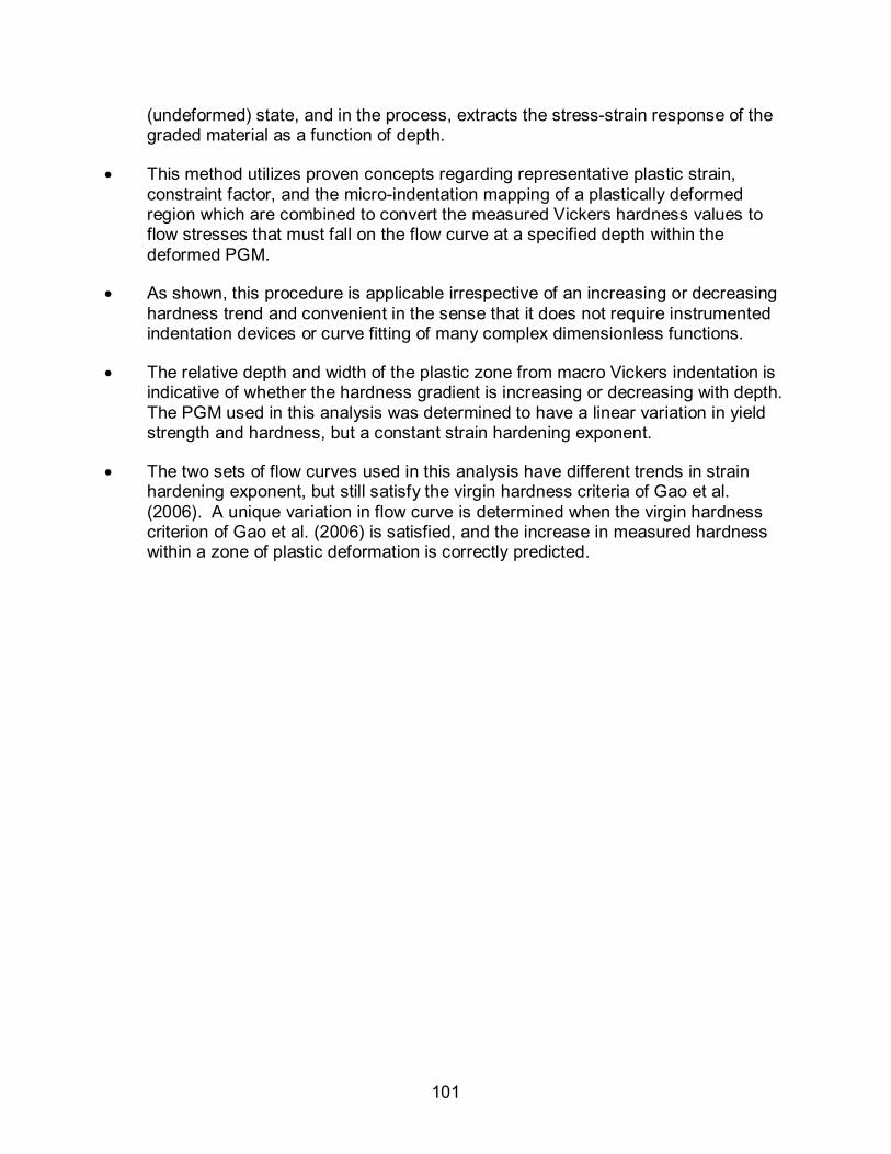
101
(undeformed) state, and in the process, extracts the stress-strain response of the graded material as a function of depth.
• This method utilizes proven concepts regarding representative plastic strain, constraint factor, and the micro-indentation mapping of a plastically deformed region which are combined to convert the measured Vickers hardness values to flow stresses that must fall on the flow curve at a specified depth within the deformed PGM.
• As shown, this procedure is applicable irrespective of an increasing or decreasing hardness trend and convenient in the sense that it does not require instrumented indentation devices or curve fitting of many complex dimensionless functions.
• The relative depth and width of the plastic zone from macro Vickers indentation is indicative of whether the hardness gradient is increasing or decreasing with depth. The PGM used in this analysis was determined to have a linear variation in yield strength and hardness, but a constant strain hardening exponent.
• The two sets of flow curves used in this analysis have different trends in strain hardening exponent, but still satisfy the virgin hardness criteria of Gao et al. (2006). A unique variation in flow curve is determined when the virgin hardness criterion of Gao et al. (2006) is satisfied, and the increase in measured hardness within a zone of plastic deformation is correctly predicted.
102
CHAPTER 6 REVERSE ANALYSIS
Nongraded Materials
As discussed in Chapters 4 and 5, the relationship between hardness and yield
strength has been given considerable attention since the time of (Tabor, 1970) as seen
by the numerous methods and applications for determining material properties.
Hardness measurements are relatively easy to perform, can be used multiple times on a
single specimen, and prevent the time-consuming tasks of creating tensile or
compression test specimens to obtain the desired yield strength of a material. Chapter
4 discussed concepts regarding the hardness of a material increases with plastic strain
and can be related to the increased yield strength (flow stress) of the plastically
deformed material. Those concepts were then applied in Chapter 5 to determine the
plastic response of graded materials when the plastic response of the core region was
known a priori.
Some materials such as plastically graded materials, coatings, and thin films are
difficult to procure traditional tensile or compression test specimens to obtain its stress-
strain curve to a desired amount of plastic strain. However, the material properties of
these materials must be known to contribute to the engineering design process for their
specific purpose. Thus new methods that are inexpensive and easy to perform are
needed to extract the flow curve of these types of materials. The process of using
indentation hardness measurements to determine the stress-strain response of a
material is called a reverse analysis. The opposite case, where an increase in hardness
with plastic strain can be predicted when the flow curve of the material is known, is
called a forward analysis and much easier to perform as shown in Chapter 4.
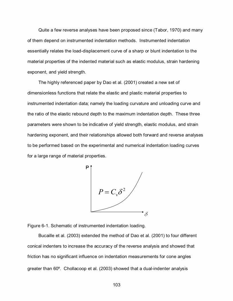
103
Quite a few reverse analyses have been proposed since (Tabor, 1970) and many
of them depend on instrumented indentation methods. Instrumented indentation
essentially relates the load-displacement curve of a sharp or blunt indentation to the
material properties of the indented material such as elastic modulus, strain hardening
exponent, and yield strength.
The highly referenced paper by Dao et al. (2001) created a new set of
dimensionless functions that relate the elastic and plastic material properties to
instrumented indentation data; namely the loading curvature and unloading curve and
the ratio of the elastic rebound depth to the maximum indentation depth. These three
parameters were shown to be indicative of yield strength, elastic modulus, and strain
hardening exponent, and their relationships allowed both forward and reverse analyses
to be performed based on the experimental and numerical indentation loading curves
for a large range of material properties.
PP
2vP C δ=
Figure 6-1. Schematic of instrumented indentation loading.
Bucaille et al. (2003) extended the method of Dao et al. (2001) to four different
conical indenters to increase the accuracy of the reverse analysis and showed that
friction has no significant influence on indentation measurements for cone angles
greater than 60⁰. Chollacoop et al. (2003) showed that a dual-indenter analysis

104
improves the uniqueness and sensitivity of the forward and reverse analyses for
instrumented indentation.
Later, the single-indenter reverse analyses by Tho et al. (2005) and Antunes et
al. (2007) determined a unique solution of material properties using instrumented
indentation provided the elastic modulus is known a priori. There are some downsides
to the instrumented indentation method such as imperfections of the indent tip which
can affect measurements at low loads, determining the “zero point” or initial contact of
the indenter, taking into account the compliance of the frame, and “pile-up” or “sink-in”
which affect indentation depth measurements Fischer-Cripps (2006). It has been
shown that different flow curves can produce the same indentation response (Tho et al.,
2005; Chollacoop et al., 2003). Also the actual plastic deformation beneath a Vickers
indent is not being investigated in these methods.
The method presented here does not require instrumented indentation devices
and will forgo the cumbersome process of creating dimensionless functions. It will use
the actual hardness measurements of a plastically deformed material to determine its
flow curve while knowing only the virgin hardness of the material and its elastic
modulus. This method will utilize the expanding cavity model derived by Gao et al.
(2006) which determined the relationship between virgin hardness, strain hardening
exponent, elastic modulus, and yield strength for strain hardening materials. The plastic
strains that correspond to a given flow stress (and hardness) will be determined by finite
element modeling described later.
To induce a gradient in plastic strain, macro Vickers indents are chosen due to
their availability and ease of use. The plastic deformation that exists within the plastic

105
zone of a Vickers indent on a ductile material allows large plastic strains to develop
without the onset of cracking due to the confinement of the surrounding material and the
large compressive hydrostatic stresses that exist in this region. This being so, the
material is allowed to strain harden to relatively large flow stresses without failure. The
resulting increase in yield strength can be captured by micro-Vickers indentation
hardness measurements on this plastically deformed region which is described next.
Experimental
The core region of commercially available Pyrowear 675 (P675) stainless steel
was used in this analysis. It has an elastic modulus of approximately 180 GPa and
virgin hardness of 433 Hv. In order to obtain a gradient in plastic strain, a macro
Vickers indent was performed on the surface of the specimen at 204 Kg indentation
load and an average diagonal length of 935µm. The resulting hardness is 433 Hv and
similar to that of the micro Vickers hardness values performed later, thus there is very
little indentation size effect (ISE) for this material and indent load range.
The macro Vickers indent was sectioned and polished to the indent diagonals
which correspond to the maximum indent and plastic zone depth. Standard
metallographic polishing procedures were used to prevent the residual stress
accumulation and additional plastic deformation induced by polishing (ASM Handbook,
2009).
Micro Vickers indentations were then performed along the centerline of this macro
indent’s plastic zone to measure the increase in hardness as shown in Figure 6-2. The
centerline is chosen because this is the deepest region of the plastic zone caused by
the macro indent and maximizes the number of data points obtained by the micro
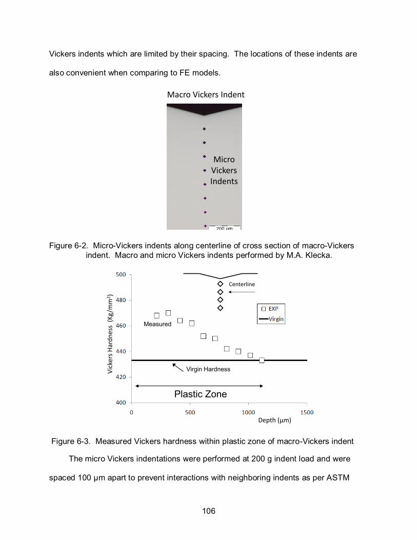
106
Vickers indents which are limited by their spacing. The locations of these indents are
also convenient when comparing to FE models.
Macro Vickers Indent
Micro Vickers Indents
Figure 6-2. Micro-Vickers indents along centerline of cross section of macro-Vickers indent. Macro and micro Vickers indents performed by M.A. Klecka.
Depth (µm)
Vick
ers
Har
dnes
s (K
g/m
m2 )
Virgin Hardness
Measured
Centerline
Plastic Zone
Figure 6-3. Measured Vickers hardness within plastic zone of macro-Vickers indent
The micro Vickers indentations were performed at 200 g indent load and were
spaced 100 µm apart to prevent interactions with neighboring indents as per ASTM
107
E384 standard. Since this is a ductile steel material, the plastic strain is well contained
within the plastic zone, thus no cracks emanate from the corners of the indents and
affect neighboring indents.
The micro Vickers indentations were simulated in FE models in Chapter 4 and
showed that the plastic zones were sufficiently small enough to prevent interactions with
neighboring indents. The measured increase in hardness along the centerline is plotted
in Figure 6-3 with respect to its virgin hardness of 433 Hv.
The highest hardness value is 215 µm from the surface and has a value of 470 Hv.
Note the increase in hardness within the plastic zone is due to the strain hardening of
the material that occurs from plastic deformation. The highest increase in hardness is in
the same region as the highest plastic strain magnitude, both of which decrease as they
approach the elastic-plastic zone boundary.
The centerline of the plastic zone has the largest usable plastic strain gradient and
the location of which is easy to identify when comparing to finite element models. It is
possible to perform the same micro Vickers indentation process on a different type of
plastically deformed region that was induced by compression, tension, torsion, or
bending, but Vickers indentation is chosen due to its large gradient in plastic strain in a
relatively small and manageable volume.
Analysis
The challenge now is to determine the flow curve of this material from the virgin
hardness, elastic modulus, and increase in hardness within a region of plastic
deformation. The expanding cavity model for strain hardening materials developed by
Gao et al. (2006) determined the relationship between hardness, yield strength, strain
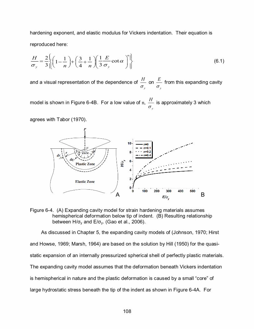
108
hardening exponent, and elastic modulus for Vickers indentation. Their equation is
reproduced here:
12 1 3 1 cot1 33 4
n
yy
EHn n
ασσ
= +− +
(6.1)
and a visual representation of the dependence of y
Hσ
on y
Eσ
from this expanding cavity
model is shown in Figure 6-4B. For a low value of n, y
Hσ
is approximately 3 which
agrees with Tabor (1970).
A B
Figure 6-4. (A) Expanding cavity model for strain hardening materials assumes hemispherical deformation below tip of indent. (B) Resulting relationship between H/σy and E/σy. (Gao et al., 2006).
As discussed in Chapter 5, the expanding cavity models of (Johnson, 1970; Hirst
and Howse, 1969; Marsh, 1964) are based on the solution by Hill (1950) for the quasi-
static expansion of an internally pressurized spherical shell of perfectly plastic materials.
The expanding cavity model assumes that the deformation beneath Vickers indentation
is hemispherical in nature and the plastic deformation is caused by a small “core” of
large hydrostatic stress beneath the tip of the indent as shown in Figure 6-4A. For
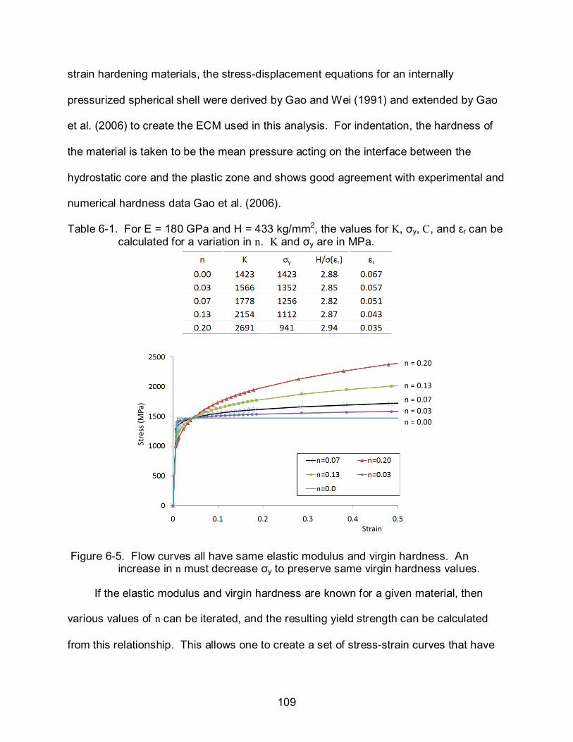
109
strain hardening materials, the stress-displacement equations for an internally
pressurized spherical shell were derived by Gao and Wei (1991) and extended by Gao
et al. (2006) to create the ECM used in this analysis. For indentation, the hardness of
the material is taken to be the mean pressure acting on the interface between the
hydrostatic core and the plastic zone and shows good agreement with experimental and
numerical hardness data Gao et al. (2006).
Table 6-1. For E = 180 GPa and H = 433 kg/mm2, the values for K, σy, C, and εr can be calculated for a variation in n. K and σy are in MPa.
Strain
Stre
ss (M
Pa)
n = 0.00n = 0.03n = 0.07
n = 0.13
n = 0.20
Figure 6-5. Flow curves all have same elastic modulus and virgin hardness. An increase in n must decrease σy to preserve same virgin hardness values.
If the elastic modulus and virgin hardness are known for a given material, then
various values of n can be iterated, and the resulting yield strength can be calculated
from this relationship. This allows one to create a set of stress-strain curves that have
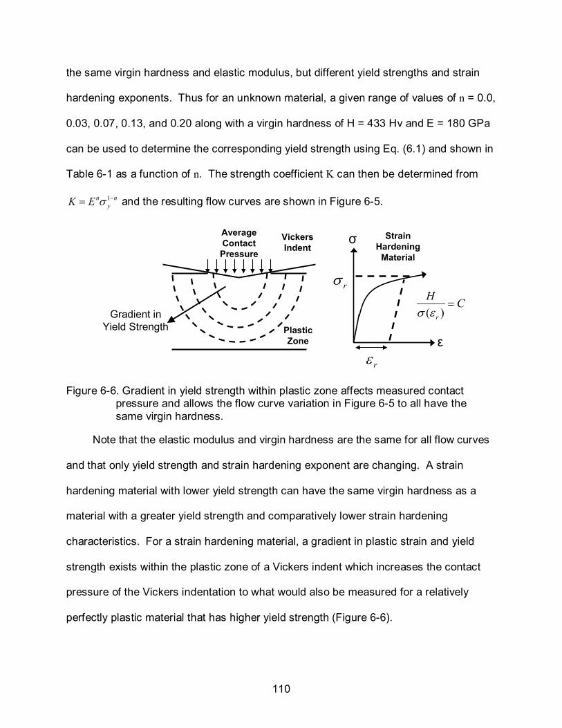
110
the same virgin hardness and elastic modulus, but different yield strengths and strain
hardening exponents. Thus for an unknown material, a given range of values of n = 0.0,
0.03, 0.07, 0.13, and 0.20 along with a virgin hardness of H = 433 Hv and E = 180 GPa
can be used to determine the corresponding yield strength using Eq. (6.1) and shown in
Table 6-1 as a function of n. The strength coefficient K can then be determined from
1n nyK E σ −= and the resulting flow curves are shown in Figure 6-5.
Plastic Zone
Strain Hardening
Material
Average Contact Pressure
Vickers Indent
σ
Gradient in Yield Strength
ε
rσ
rε
( )r
H Cσ ε
=
Figure 6-6. Gradient in yield strength within plastic zone affects measured contact pressure and allows the flow curve variation in Figure 6-5 to all have the same virgin hardness.
Note that the elastic modulus and virgin hardness are the same for all flow curves
and that only yield strength and strain hardening exponent are changing. A strain
hardening material with lower yield strength can have the same virgin hardness as a
material with a greater yield strength and comparatively lower strain hardening
characteristics. For a strain hardening material, a gradient in plastic strain and yield
strength exists within the plastic zone of a Vickers indent which increases the contact
pressure of the Vickers indentation to what would also be measured for a relatively
perfectly plastic material that has higher yield strength (Figure 6-6).
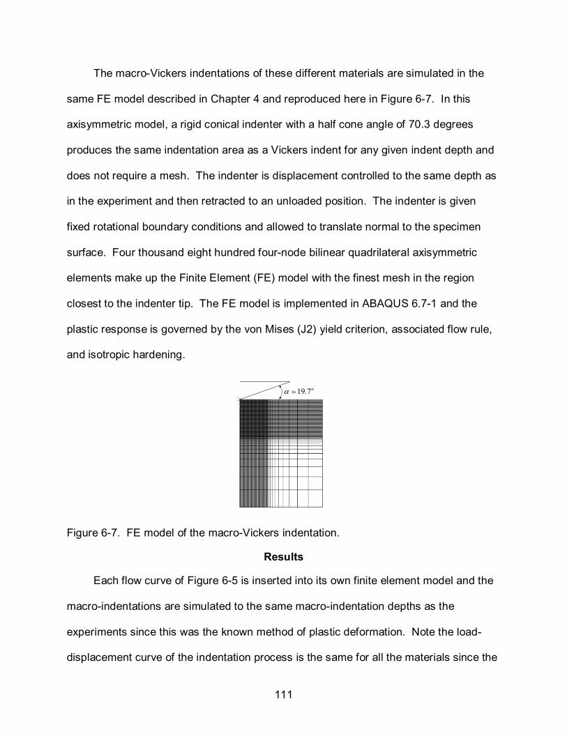
111
The macro-Vickers indentations of these different materials are simulated in the
same FE model described in Chapter 4 and reproduced here in Figure 6-7. In this
axisymmetric model, a rigid conical indenter with a half cone angle of 70.3 degrees
produces the same indentation area as a Vickers indent for any given indent depth and
does not require a mesh. The indenter is displacement controlled to the same depth as
in the experiment and then retracted to an unloaded position. The indenter is given
fixed rotational boundary conditions and allowed to translate normal to the specimen
surface. Four thousand eight hundred four-node bilinear quadrilateral axisymmetric
elements make up the Finite Element (FE) model with the finest mesh in the region
closest to the indenter tip. The FE model is implemented in ABAQUS 6.7-1 and the
plastic response is governed by the von Mises (J2) yield criterion, associated flow rule,
and isotropic hardening.
o19.7α =
Figure 6-7. FE model of the macro-Vickers indentation.
Results
Each flow curve of Figure 6-5 is inserted into its own finite element model and the
macro-indentations are simulated to the same macro-indentation depths as the
experiments since this was the known method of plastic deformation. Note the load-
displacement curve of the indentation process is the same for all the materials since the

112
virgin hardness is the same for each and independent of indentation depth as shown in
Figure 6-8. Similar load displacement curves as the one shown here were used in the
previously mentioned methods to determine the material properties of the indented
materials. This information is not necessary for this analysis, but only shown here to
demonstrate that different flow curves can produce the same indentation loading curve
because the virgin hardness is independent of depth and the same for the material test
cases shown here.
Indentation Depth (mm)
Inde
ntat
ion
Load
(Kg)
Figure 6-8. Load displacement curve from FE model is the same for all flow curves since virgin hardness is same for all and hardness is independent of indent depth.
The plastic strains below the indent tip and along the centerlines of the plastic
zones of all material test cases are calculated by the FE model and shown in Figure 6-
9. Note they are all similar in magnitude and distribution with minor variations between
them. This is to be expected since the gradient in flow stress within the plastic zone will
not be the same for the different strain hardening materials.

113
The modified Tabor’s rule that was introduced in Chapter 4 is then repeated for
each flow curve via ( )r pH Cσ ε ε= + in order to predict the increase in hardness within
the plastic zone of each material where rε is the representative plastic strain induced by
the micro-Vickers indentation process, pε is the equivalent plastic strain at a specific
point within the gradient (Figure 6-9), and C is the Constraint factor, ( )r
HCσ ε
= .
The representative strain used in this analysis is the average volumetric plastic
strain induced by Vickers indentation that was shown to be dependent only on the strain
hardening exponent by Jayaraman et al. (1998). The representative plastic strain takes
into account the additional strain hardening due to the plastic deformation of the micro-
indentation process itself.
Depth (mm)
Equi
vale
nt P
last
ic S
trai
n
Figure 6-9. Plastic strain gradient along centerline of plastic zone for all material test cases.
Values for the average plastic strain induced by a Vickers indent are shown in
Figure 6-10 and taken from Jayaraman et al. (1998). This average plastic strain was
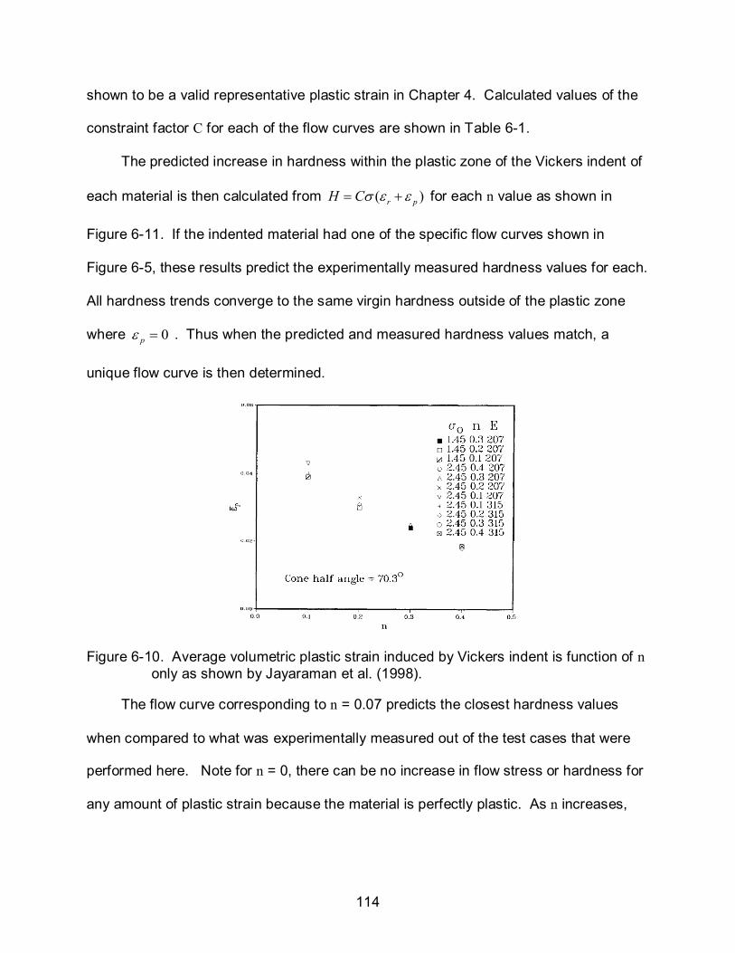
114
shown to be a valid representative plastic strain in Chapter 4. Calculated values of the
constraint factor C for each of the flow curves are shown in Table 6-1.
The predicted increase in hardness within the plastic zone of the Vickers indent of
each material is then calculated from ( )r pH Cσ ε ε= + for each n value as shown in
Figure 6-11. If the indented material had one of the specific flow curves shown in
Figure 6-5, these results predict the experimentally measured hardness values for each.
All hardness trends converge to the same virgin hardness outside of the plastic zone
where 0pε = . Thus when the predicted and measured hardness values match, a
unique flow curve is then determined.
Figure 6-10. Average volumetric plastic strain induced by Vickers indent is function of n only as shown by Jayaraman et al. (1998).
The flow curve corresponding to n = 0.07 predicts the closest hardness values
when compared to what was experimentally measured out of the test cases that were
performed here. Note for n = 0, there can be no increase in flow stress or hardness for
any amount of plastic strain because the material is perfectly plastic. As n increases,

115
the change in hardness also increases for a given amount of plastic strain, the
distributions of which were shown to be similar for all materials in Figure 6-9.
Depth (µm)
Vick
ers
Har
dnes
s (K
g/m
m2 )
n = 0
n = 0.03
n = 0.07
n = 0.13n = 0.20
Virgin Hardness
Measured
Figure 6-11. Predicted hardness values within plastic zone of macro-Vickers indents. Note all converge to virgin hardness value, but different values for n lead to different increases in hardness for the same macro indent depth.
0.0641800σ ε=
Figure 6-12. Compression test of P675 core region results in power law curve fit with strength coefficient K = 1800 MPa and strain hardening exponent n = 0.064 and close to what the method predicted. Compression test performed by M.A. Klecka.
To check the validity of this method, a compression test was performed on the
core region of the P675 stainless steel. The ample amount of core material available
allows for a compression test specimen of 10 mm x 6 mm x 3.175 mm to be extracted.
116
The compression test was conducted in a MTS load frame up to a failure strain of 0.27.
The power-law curve fit, nKσ ε= , applied to the flow curve obtained from this
compression test shown in Figure 6-12 resulted in a strength coefficient K = 1800 MPa
and a strain hardening exponent n = 0.064 which is close to the K = 1778 and n = 0.07
that was predicted by the method.
Key Points
The results of this analysis have been submitted for peer review for publication in
Acta Materialia and the key points of which are summarized here:
• A reverse analysis that predicts the flow behavior of a material based on indentation hardness measurements was presented that utilizes the well established procedures of expanding cavity models, Tabor’s rule of converting hardness to flow stress for a given amount of plastic deformation, and representative plastic strain of the indentation process.
• A unique solution for yield strength and strain hardening exponent is determined when the predicted and measured hardness values match over a plastically deformed region. It is unique in the sense that the values for n and σy must satisfy the virgin hardness relationship derived by Gao et al. (2006) and match the experimentally-measured increase in hardness in a plastically deformed region.
• The problems with uniqueness of single-indenter reverse analyses that relied on instrumented indentation devices were often solved when the elastic modulus of the indented material was known a priori (Tho et al., 2005; Antunes et al., 2007). This is similar to this analysis where the elastic modulus must be known in order to determine the yield strength and strain hardening exponent from the ECM of Gao et al. (2006). This method is not limited to analyzing the deformation induced by Vickers indentation, but can be used for any plastically deformed region provided the plastic strain magnitude and distribution can be determined by finite element modeling.
• These findings will be used to determine the plastic response of case hardened M50 NiL in the next section of this Chapter which is needed for the spall edge impact analysis of Chapter 7.
Reverse Analysis Graded Materials
The reverse analysis for non-graded materials can be applied to graded materials
as well. In this analysis the graded material properties of case hardened M50 NiL will
117
be determined without knowing the core material properties a priori. Thus, the lower
bound of possible plastic behavior is initially unknown. The method presented here will
prevent the laborious task of extracting and preparing a tensile test specimen of the
core or substrate region. A similar indentation method to that used in Chapter 5 for
P675 steel is repeated here for M50NiL steel without the compression test of the core
region. The plastic response of M50NiL is needed to repeat the ball-spall edge impact
study in Chapter 7 using its specific gradient in plastic response to determine its affect
on the magnitude or distribution of residual tensile stress and plastic strain and
consequently spall propagation rate.
Experimental
Commercially available, case hardened M50 NiL is the PGM used in this analysis.
The M50 NiL samples were extracted from disks donated by AFRL that were originally
intended for ball-on-disk wear testing. Specimens were sectioned, ground, and
polished on surfaces parallel to the carbon gradient. Standard metallographic polishing
procedures which use progressively finer polishing media were used to minimize
damage and residual stresses induced by polishing (ASM Handbook, 2009).
Micro Vickers-indentations were conducted on this cross-section using a Wilson®
Instruments (Tukon ™ 2100B) Vickers indenter at 200g indent loads for 15 seconds
loading duration. The indents were spaced 2.5 times the indent diagonal to prevent
interactions with neighboring indents as per ASTM E384 standard. This was similar to
the indentation procedures used in Chapters 4 and 5. The Vickers hardness profile in
Figure 6-13 for the virgin M50 NiL steel displays a nonlinear trend in virgin hardness
that varies from 820 Hv at the surface to 455 Hv over a depth of 2.5 mm. Note that the
surface hardness is lower than that of P675 steel (930 Hv) as shown in Chapter 5;
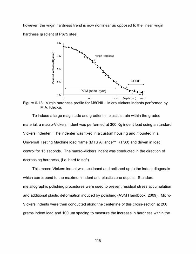
118
however, the virgin hardness trend is now nonlinear as opposed to the linear virgin
hardness gradient of P675 steel.
Depth (µm)
Vic
kers
Har
dnes
s (K
g/m
m2 )
Virgin Hardness
PGM (case layer)
CORE
Depth (µm)
Vic
kers
Har
dnes
s (K
g/m
m2 )
Virgin Hardness
PGM (case layer)
CORE
Figure 6-13. Virgin hardness profile for M50NiL. Micro Vickers indents performed by
M.A. Klecka.
To induce a large magnitude and gradient in plastic strain within the graded
material, a macro-Vickers indent was performed at 300 Kg indent load using a standard
Vickers indenter. The indenter was fixed in a custom housing and mounted in a
Universal Testing Machine load frame (MTS Alliance™ RT/30) and driven in load
control for 15 seconds. The macro-Vickers indent was conducted in the direction of
decreasing hardness, (i.e. hard to soft).
This macro-Vickers indent was sectioned and polished up to the indent diagonals
which correspond to the maximum indent and plastic zone depths. Standard
metallographic polishing procedures were used to prevent residual stress accumulation
and additional plastic deformation induced by polishing (ASM Handbook, 2009). Micro-
Vickers indents were then conducted along the centerline of this cross-section at 200
grams indent load and 100 µm spacing to measure the increase in hardness within the
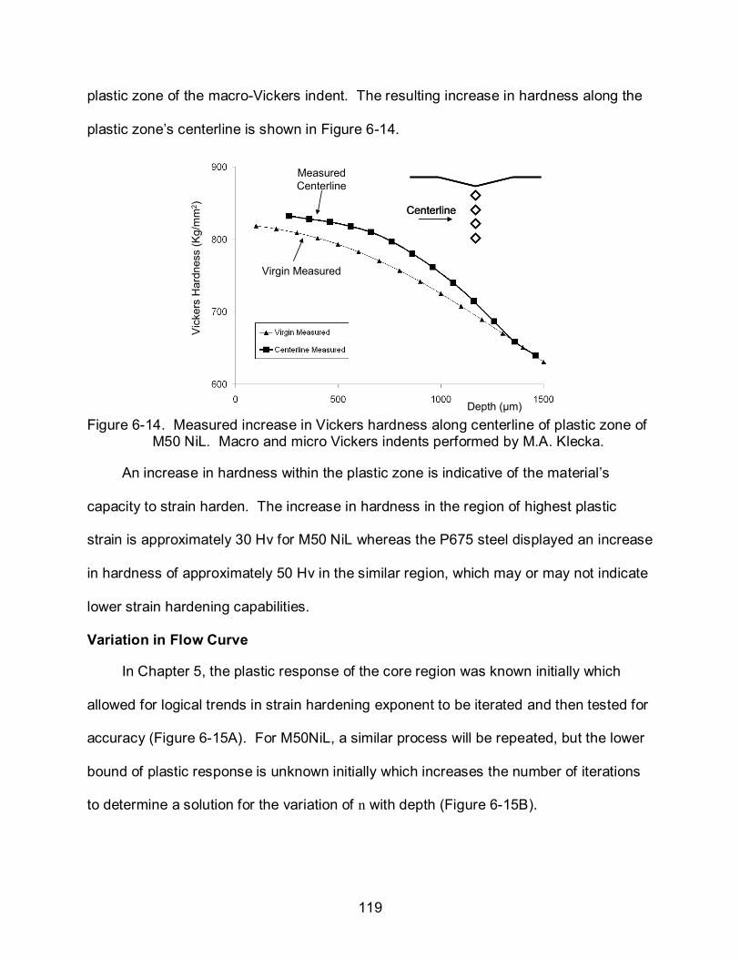
119
plastic zone of the macro-Vickers indent. The resulting increase in hardness along the
plastic zone’s centerline is shown in Figure 6-14.
Depth (µm)
Vic
kers
Har
dnes
s (K
g/m
m2 )
Virgin Measured
Measured Centerline
CenterlineCenterline
Figure 6-14. Measured increase in Vickers hardness along centerline of plastic zone of
M50 NiL. Macro and micro Vickers indents performed by M.A. Klecka.
An increase in hardness within the plastic zone is indicative of the material’s
capacity to strain harden. The increase in hardness in the region of highest plastic
strain is approximately 30 Hv for M50 NiL whereas the P675 steel displayed an increase
in hardness of approximately 50 Hv in the similar region, which may or may not indicate
lower strain hardening capabilities.
Variation in Flow Curve
In Chapter 5, the plastic response of the core region was known initially which
allowed for logical trends in strain hardening exponent to be iterated and then tested for
accuracy (Figure 6-15A). For M50NiL, a similar process will be repeated, but the lower
bound of plastic response is unknown initially which increases the number of iterations
to determine a solution for the variation of n with depth (Figure 6-15B).
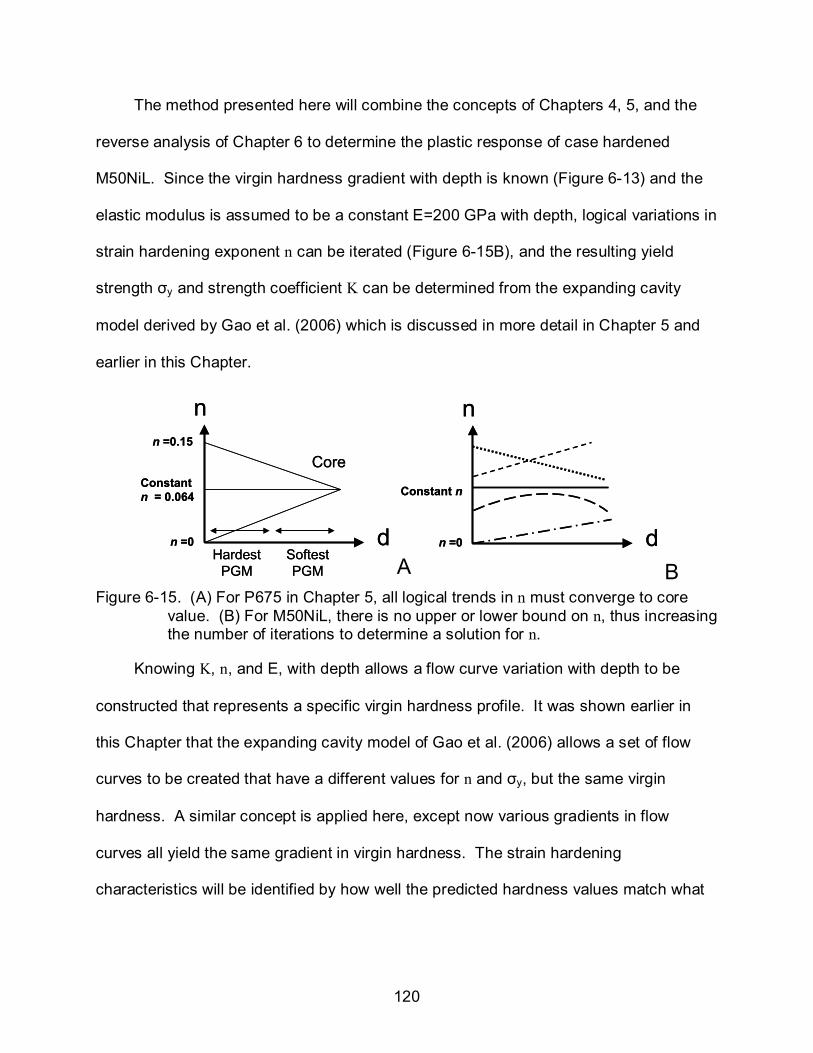
120
The method presented here will combine the concepts of Chapters 4, 5, and the
reverse analysis of Chapter 6 to determine the plastic response of case hardened
M50NiL. Since the virgin hardness gradient with depth is known (Figure 6-13) and the
elastic modulus is assumed to be a constant E=200 GPa with depth, logical variations in
strain hardening exponent n can be iterated (Figure 6-15B), and the resulting yield
strength σy and strength coefficient K can be determined from the expanding cavity
model derived by Gao et al. (2006) which is discussed in more detail in Chapter 5 and
earlier in this Chapter.
n
d
Core
Hardest PGM
Softest PGM
Constant n = 0.064
n =0
n =0.15
n
d n =0
Constant n
n
d
Core
Hardest PGM
Softest PGM
Constant n = 0.064
n =0
n =0.15
n
d n =0
Constant n
A B
Figure 6-15. (A) For P675 in Chapter 5, all logical trends in n must converge to core value. (B) For M50NiL, there is no upper or lower bound on n, thus increasing the number of iterations to determine a solution for n.
Knowing K, n, and E, with depth allows a flow curve variation with depth to be
constructed that represents a specific virgin hardness profile. It was shown earlier in
this Chapter that the expanding cavity model of Gao et al. (2006) allows a set of flow
curves to be created that have a different values for n and σy, but the same virgin
hardness. A similar concept is applied here, except now various gradients in flow
curves all yield the same gradient in virgin hardness. The strain hardening
characteristics will be identified by how well the predicted hardness values match what

121
was actually measured in a region of plastic deformation as was similarly done by the
reverse analysis for nongraded materials earlier in this Chapter.
Depth (µm)Depth (µm)
Stra
in H
arde
ning
Exp
onen
t n
K o
r σy
(MP
a)
A B Figure 6-16. (A) Constant strain hardening exponent with depth as two initial test cases.
(B) Resulting yield strength and strength coefficient as functions of depth and determined by ECM of Gao et al. (2006).
n = 0.10 constant
Strain
n = 0.05 constant
Strain
Stre
ss (M
Pa)
Stre
ss (M
Pa)
A B Figure 6-17. Flow curve variation for M50 NiL virgin hardness trend when (A) n =0.05
and (B) n = 0.10. The flow curves shown correspond to the following depths, 0 (surface), 200, 400, 600, and 800 µm. The surface flow curve has the highest value for yield strength and strength coefficient, and decreases with depth.
As a first step, two test cases of constant n = 0.05 and n = 0.10 with depth is
assumed since a similar trend provided adequate results for P675 steel of Chapter 5
and shown in Figure 6-16A for M50NiL. The expanding cavity model (ECM) determined
the relationship between hardness, yield strength, elastic modulus, and strain hardening
exponent by equation 6.1 is then used to determine the resulting yield strength and
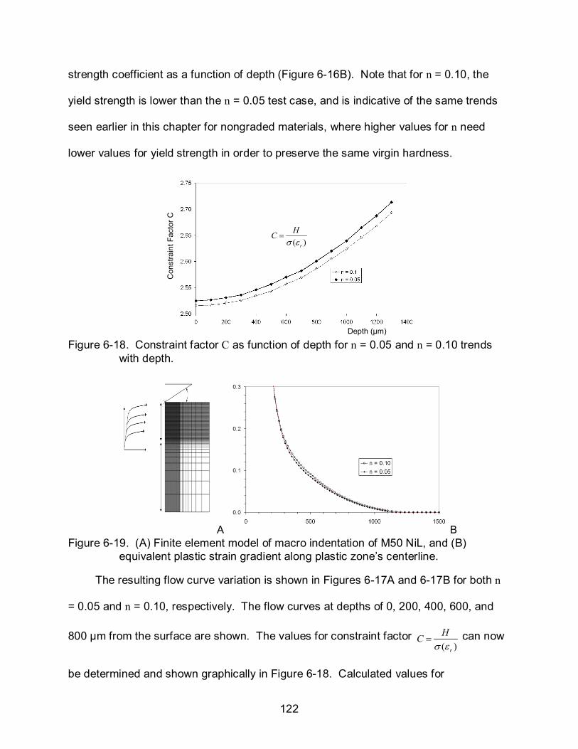
122
strength coefficient as a function of depth (Figure 6-16B). Note that for n = 0.10, the
yield strength is lower than the n = 0.05 test case, and is indicative of the same trends
seen earlier in this chapter for nongraded materials, where higher values for n need
lower values for yield strength in order to preserve the same virgin hardness.
Depth (µm)
Con
stra
int F
acto
r C
( )r
HCσ ε
=
Figure 6-18. Constraint factor C as function of depth for n = 0.05 and n = 0.10 trends
with depth.
(a) (b)A B
Figure 6-19. (A) Finite element model of macro indentation of M50 NiL, and (B) equivalent plastic strain gradient along plastic zone’s centerline.
The resulting flow curve variation is shown in Figures 6-17A and 6-17B for both n
= 0.05 and n = 0.10, respectively. The flow curves at depths of 0, 200, 400, 600, and
800 µm from the surface are shown. The values for constraint factor ( )r
HCσ ε
= can now
be determined and shown graphically in Figure 6-18. Calculated values for
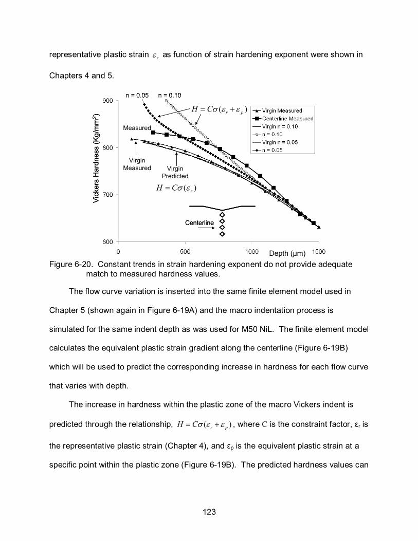
123
representative plastic strain rε as function of strain hardening exponent were shown in
Chapters 4 and 5.
Depth (µm)
Vic
kers
Har
dnes
s (K
g/m
m2 )
Virgin Measured
Centerline
Virgin Predicted
( )rH Cσ ε=
( )r pH Cσ ε ε= +
n = 0.05 n = 0.10
Measured
Depth (µm)
Vic
kers
Har
dnes
s (K
g/m
m2 )
Virgin Measured
CenterlineCenterline
Virgin Predicted
( )rH Cσ ε=
( )r pH Cσ ε ε= +
n = 0.05 n = 0.10
Measured
Figure 6-20. Constant trends in strain hardening exponent do not provide adequate
match to measured hardness values.
The flow curve variation is inserted into the same finite element model used in
Chapter 5 (shown again in Figure 6-19A) and the macro indentation process is
simulated for the same indent depth as was used for M50 NiL. The finite element model
calculates the equivalent plastic strain gradient along the centerline (Figure 6-19B)
which will be used to predict the corresponding increase in hardness for each flow curve
that varies with depth.
The increase in hardness within the plastic zone of the macro Vickers indent is
predicted through the relationship, ( )r pH Cσ ε ε= + , where C is the constraint factor, εr is
the representative plastic strain (Chapter 4), and εp is the equivalent plastic strain at a
specific point within the plastic zone (Figure 6-19B). The predicted hardness values can
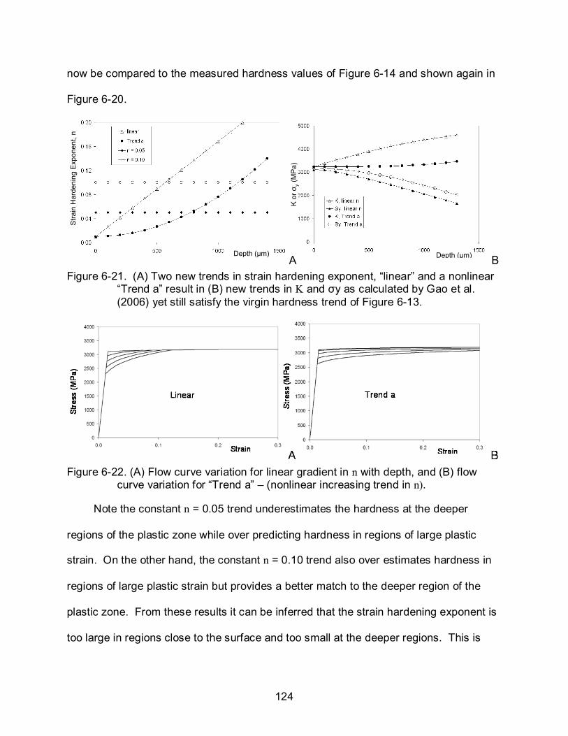
124
now be compared to the measured hardness values of Figure 6-14 and shown again in
Figure 6-20.
Depth (µm)
Stra
in H
arde
ning
Exp
onen
t, n
( )
K o
r σy
(MP
a)
Depth (µm)A B Figure 6-21. (A) Two new trends in strain hardening exponent, “linear” and a nonlinear
“Trend a” result in (B) new trends in K and σy as calculated by Gao et al. (2006) yet still satisfy the virgin hardness trend of Figure 6-13.
Figure 6-22. (A) Flow curve variation for linear gradient in n with depth, and (B) flow
curve variation for “Trend a” – (nonlinear increasing trend in n).
Note the constant n = 0.05 trend underestimates the hardness at the deeper
regions of the plastic zone while over predicting hardness in regions of large plastic
strain. On the other hand, the constant n = 0.10 trend also over estimates hardness in
regions of large plastic strain but provides a better match to the deeper region of the
plastic zone. From these results it can be inferred that the strain hardening exponent is
too large in regions close to the surface and too small at the deeper regions. This is
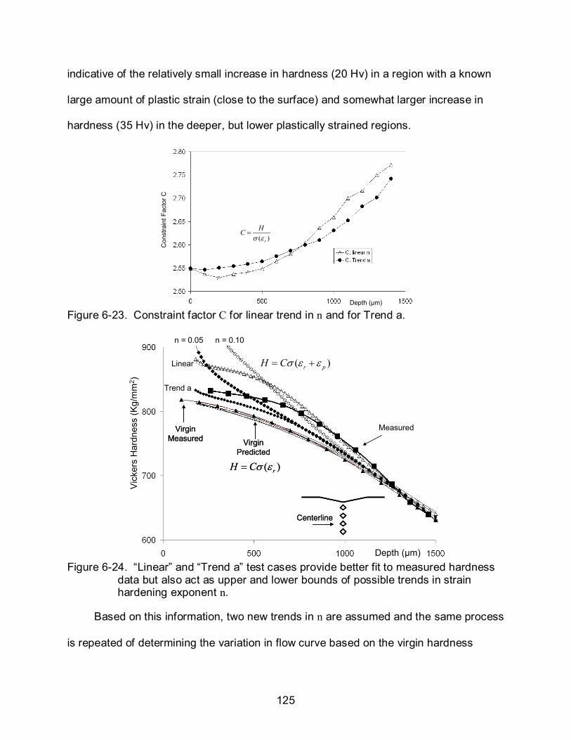
125
indicative of the relatively small increase in hardness (20 Hv) in a region with a known
large amount of plastic strain (close to the surface) and somewhat larger increase in
hardness (35 Hv) in the deeper, but lower plastically strained regions.
Depth (µm)
Con
stra
int F
acto
r C
( )r
HCσ ε
=
Figure 6-23. Constraint factor C for linear trend in n and for Trend a.
Depth (µm)
Vic
kers
Har
dnes
s (K
g/m
m2 )
Virgin Measured
Virgin Measured
CenterlineCenterline
Virgin Predicted
( )rH Cσ ε=
Virgin Predicted
( )rH Cσ ε=
( )r pH Cσ ε ε= +
n = 0.05 n = 0.10
Linear
Trend a
Measured
Figure 6-24. “Linear” and “Trend a” test cases provide better fit to measured hardness
data but also act as upper and lower bounds of possible trends in strain hardening exponent n.
Based on this information, two new trends in n are assumed and the same process
is repeated of determining the variation in flow curve based on the virgin hardness
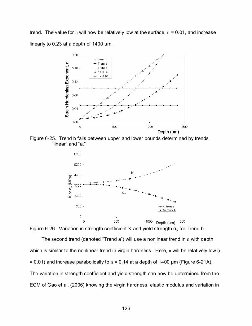
126
trend. The value for n will now be relatively low at the surface, n = 0.01, and increase
linearly to 0.23 at a depth of 1400 µm.
Depth (µm)
Stra
in H
arde
ning
Exp
onen
t, n
Depth (µm)
Stra
in H
arde
ning
Exp
onen
t, n
Figure 6-25. Trend b falls between upper and lower bounds determined by trends
“linear” and “a.”
Depth (µm)
K o
r σy
(MP
a)
K
σy
Figure 6-26. Variation in strength coefficient K and yield strength σy for Trend b.
The second trend (denoted “Trend a”) will use a nonlinear trend in n with depth
which is similar to the nonlinear trend in virgin hardness. Here, n will be relatively low (n
= 0.01) and increase parabolically to n = 0.14 at a depth of 1400 µm (Figure 6-21A).
The variation in strength coefficient and yield strength can now be determined from the
ECM of Gao et al. (2006) knowing the virgin hardness, elastic modulus and variation in
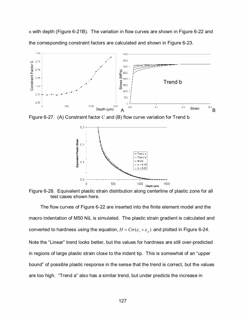
127
n with depth (Figure 6-21B). The variation in flow curves are shown in Figure 6-22 and
the corresponding constraint factors are calculated and shown in Figure 6-23.
Trend b
Strain
Stre
ss (M
Pa)
Depth (µm)
Con
stra
int F
acto
r C
(a) (b)A B Figure 6-27. (A) Constraint factor C and (B) flow curve variation for Trend b.
Depth (µm)
Equ
ival
ent P
last
ic S
train
Depth (µm)
Equ
ival
ent P
last
ic S
train
Figure 6-28. Equivalent plastic strain distribution along centerline of plastic zone for all
test cases shown here.
The flow curves of Figure 6-22 are inserted into the finite element model and the
macro indentation of M50 NiL is simulated. The plastic strain gradient is calculated and
converted to hardness using the equation, ( )r pH Cσ ε ε= + and plotted in Figure 6-24.
Note the “Linear” trend looks better, but the values for hardness are still over-predicted
in regions of large plastic strain close to the indent tip. This is somewhat of an “upper
bound” of possible plastic response in the sense that the trend is correct, but the values
are too high. “Trend a” also has a similar trend, but under predicts the increase in
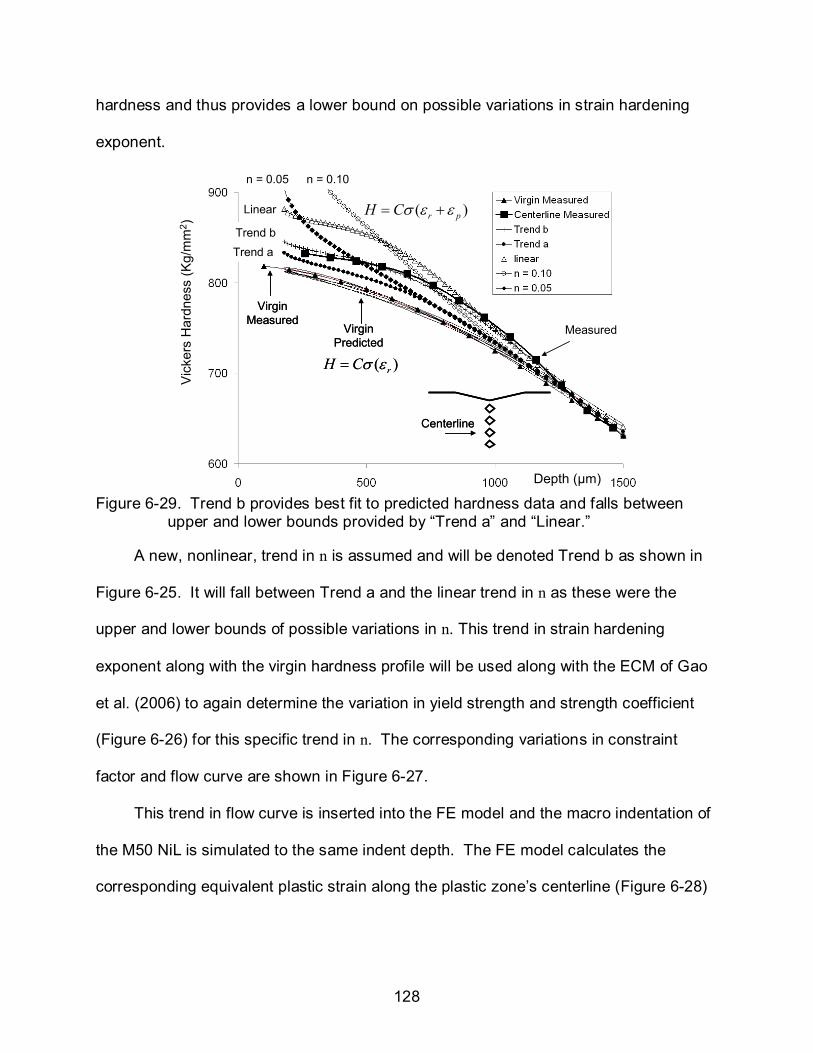
128
hardness and thus provides a lower bound on possible variations in strain hardening
exponent.
Depth (µm)
Vic
kers
Har
dnes
s (K
g/m
m2 )
Virgin Measured
Virgin Measured
CenterlineCenterline
Virgin Predicted
( )rH Cσ ε=
Virgin Predicted
( )rH Cσ ε=
( )r pH Cσ ε ε= +
n = 0.05 n = 0.10
Linear
Trend a
Measured
Trend b
Figure 6-29. Trend b provides best fit to predicted hardness data and falls between
upper and lower bounds provided by “Trend a” and “Linear.”
A new, nonlinear, trend in n is assumed and will be denoted Trend b as shown in
Figure 6-25. It will fall between Trend a and the linear trend in n as these were the
upper and lower bounds of possible variations in n. This trend in strain hardening
exponent along with the virgin hardness profile will be used along with the ECM of Gao
et al. (2006) to again determine the variation in yield strength and strength coefficient
(Figure 6-26) for this specific trend in n. The corresponding variations in constraint
factor and flow curve are shown in Figure 6-27.
This trend in flow curve is inserted into the FE model and the macro indentation of
the M50 NiL is simulated to the same indent depth. The FE model calculates the
corresponding equivalent plastic strain along the plastic zone’s centerline (Figure 6-28)

129
and this will be used along with the equation ( )r pH Cσ ε ε= + to predict the increase in
hardness within this region as shown in Figure 6-29.
Note that Trend b provides the best fit when comparing predicted and measured
hardness values along the centerline of the macro indent’s plastic zone. The equivalent
plastic strain decreases asymptotically along the plastic zone’s centerline and that all
plastic strains below a depth of 700 µm are considerably low, i.e. 0.04 or less. The
hardness measurements at these locations correspond to a flow stress on the flow
curve at that specific depth, thus the higher the plastic strain, the “farther away” the flow
stress is from its original yield strength (Figure 6-30).
σ
εεp
σ
εεp
σ
εεp
σ
εεp
Figure 6-30. The sensitivity to strain hardening exponent decreases with decreasing plastic strain in that flow curves that have similar flow stresses at low plastic strain could have entirely different plastic responses at large plastic strain that this method would not be able to predict.
In other words, this method can only predict the plastic response at any given
depth up to the maximum plastic strain that was experienced at that specific depth.
This is why the hardness measurements were performed along the centerline because
this is where the highest plastic strain occurs along a specific depth. Thus, it is possible
to have a set of flow curves that have similar plastic responses at low plastic strains, but
an entirely different plastic response at large plastic strain (Figure 6-31) and significantly
130
different n values. Caution should therefore be taken when considering the plastic
response predicted by this method for regions with low plastic strains. This is why the
flow curves at depths 0, 200, 400, 600, and 800µm were shown in this chapter and not
the flow curves for the deeper material. The plastic zone extended to 1300 µm and
trends for n, K, and σy were shown up to these depths, but these values are only valid
up to the maximum plastic strain that was experienced along their specific depths.
These material properties of Trend b will be used to repeat the spall edge impact
analysis of for M50NiL in Chapter 7.
Key Points
• A reverse analysis was presented here for plastically graded materials to determine the plastic response of case hardened M50 NiL in order to repeat a similar spall edge impact analysis of Chapter 3 for this specific material which is presented next in Chapter 7.
• The sensitivity to strain hardening exponent decreases as the maximum plastic strain experienced at a specific depth decreases. More simply, this method can only predict the plastic response up to the maximum plastic strain that was experienced at a specific depth. Plastic strains at larger depths are so small that practically any value for n would result in a predicted hardness that could provide a reasonable fit to what was experimentally measured.
• The reverse analysis for nongraded materials was essentially repeated for every depth within the plastically deformed graded material. In the nongraded reverse analysis, various values for n were assumed and tested for accuracy for a continuous, nongraded material. In the graded material reverse analysis, logical trends in n that vary with depth were tested for accuracy through the prediction of experimentally measured hardness values.
• All of the variations in flow curves that were based on an assumed variation in n reflect the same virgin hardness profile because they satisfy the condition set by Gao et al. (2006) which relates virgin hardness to strain hardening exponent, yield strength, and elastic modulus. The strain hardening characteristics were identified by the measured increase in hardness at a specific depth and the corresponding plastic strain was determined by FE modeling.
• This indentation method to determine the plastic response of graded materials is similar to that presented in Chapter 5 with the exception that the lower bound of the gradation in plastic response is initially unknown.
131
CHAPTER 7 SPALL MODELING
Spall Propagation for 52100, M50, and M50 NiL Bearing Materials
The flow curve for M50 NiL as a function of case depth that was determined in
Chapter 6 will now be used to repeat the ball-spall edge impact analysis introduced in
Chapter 3 and compared to M50 and 52100 bearing steels to determine if the FE model
can predict the differences in spall propagation characteristics of these materials. In
this analysis the magnitude and distribution of plastic strain will be indicative of the
amount of damage induced by a ball impact on a spall edge. More damage in the form
of plastic strain is expected to cause spalls to propagate sooner and faster since fatigue
crack initiation and growth is highly dependent on the extent of plastic deformation.
A concise review of the spall propagation experiments by Rosado et al. (2010) and
Chapters 1 and 3 are reprised here. Scaled versions of the bearings used in the actual
aircraft engines were tested for spall-propagation in controlled experiments at the Air
Force Research Labs, WPAFB, Ohio. The bearings were 208 size (40 mm bore) split
inner raceways with 0.5 in diameter balls. Their study investigated 52100, M50 through-
hardened, and M50 NiL case hardened bearing steels. The M50 and M50 NiL bearings
used silicon nitride balls while the 52100 bearings used 52100 steel balls. Brand new
bearings and bearings that had been subjected to as much as tens of billions of stress
cycles were both used in their study to see if initial rolling contact fatigue affected spall
propagation rate.
Figure 7-1 taken from Rosado et al. (2010) displays the mass loss from the
raceway surface for all three types of bearings as a function of millions of stress cycles
during spall propagation for new bearing raceways. These raceways were indented

132
with Rockwell C indents to act as stress risers, initiate fatigue cracks during bearing
operation, and reduce the amount of time to spall initiation. The bearings were inserted
into a test rig and operated at a maximum contact pressure of 2.41 GPa (350 ksi, as
seen on the virgin raceway surface). The mass loss from the spalled bearing was
detected by an oil debris monitor (ODM) and the average size of the spalled particles
were on the order of 100µm Rosado et al. (2010). Note 52100 bearing steel had the
shortest amount of time to spall initiation and the fastest spall propagation rate whereas
both the M50 and M50NiL steels showed the longest amount of time to spall initiation
and a slower spall propagation rate. Note the similarity in both M50 and M50 NiL with
two outliers for M50.
Figure 7-1. Spall propagation characteristics for M50, M50 NiL, and 52100 bearing steels. Spalls initiated by Rockwell C indents on virgin raceways at maximum contact pressure of 2.41 GPa (350 ksi). Rosado et al. (2010)
A similar experiment was performed with a lower contact pressure (2.10 GPa
virgin raceway (305 ksi), Figure 7-2) and as expected the amount of time to spall
propagation was considerably longer due to the lower contact stresses, but the trends
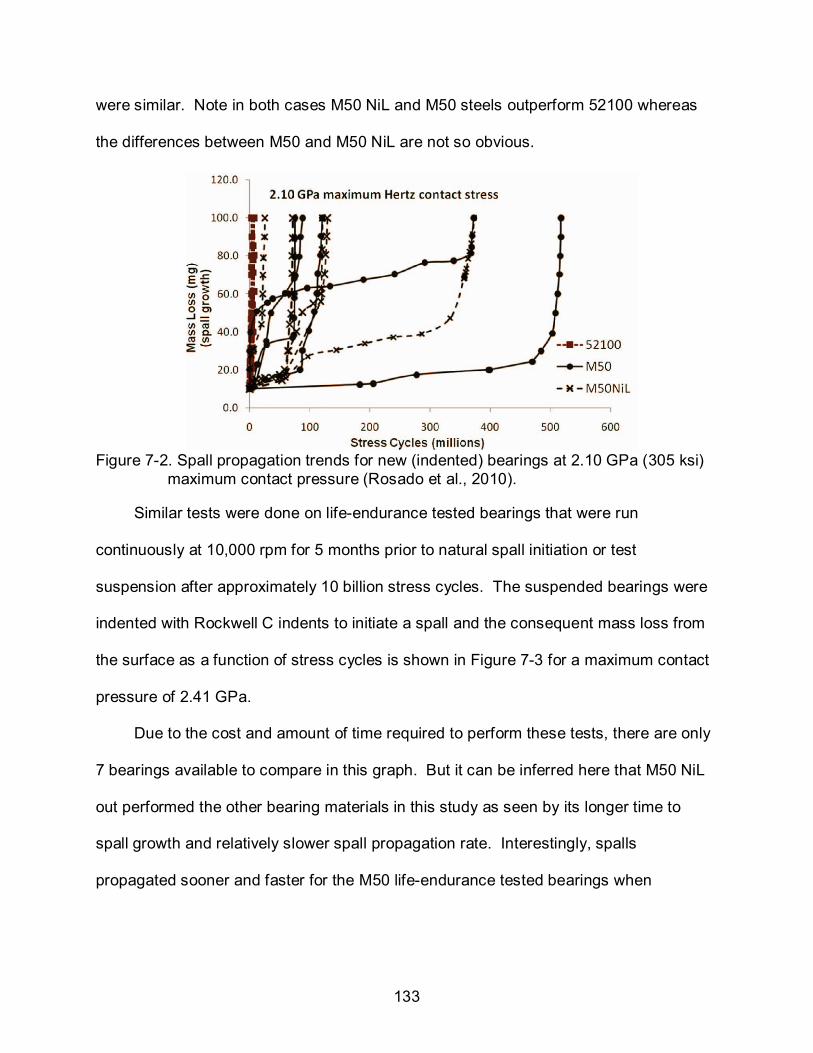
133
were similar. Note in both cases M50 NiL and M50 steels outperform 52100 whereas
the differences between M50 and M50 NiL are not so obvious.
Figure 7-2. Spall propagation trends for new (indented) bearings at 2.10 GPa (305 ksi)
maximum contact pressure (Rosado et al., 2010).
Similar tests were done on life-endurance tested bearings that were run
continuously at 10,000 rpm for 5 months prior to natural spall initiation or test
suspension after approximately 10 billion stress cycles. The suspended bearings were
indented with Rockwell C indents to initiate a spall and the consequent mass loss from
the surface as a function of stress cycles is shown in Figure 7-3 for a maximum contact
pressure of 2.41 GPa.
Due to the cost and amount of time required to perform these tests, there are only
7 bearings available to compare in this graph. But it can be inferred here that M50 NiL
out performed the other bearing materials in this study as seen by its longer time to
spall growth and relatively slower spall propagation rate. Interestingly, spalls
propagated sooner and faster for the M50 life-endurance tested bearings when
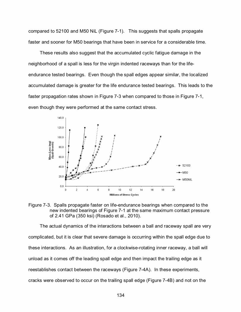
134
compared to 52100 and M50 NiL (Figure 7-1). This suggests that spalls propagate
faster and sooner for M50 bearings that have been in service for a considerable time.
These results also suggest that the accumulated cyclic fatigue damage in the
neighborhood of a spall is less for the virgin indented raceways than for the life-
endurance tested bearings. Even though the spall edges appear similar, the localized
accumulated damage is greater for the life endurance tested bearings. This leads to the
faster propagation rates shown in Figure 7-3 when compared to those in Figure 7-1,
even though they were performed at the same contact stress.
Figure 7-3. Spalls propagate faster on life-endurance bearings when compared to the new indented bearings of Figure 7-1 at the same maximum contact pressure of 2.41 GPa (350 ksi) (Rosado et al., 2010).
The actual dynamics of the interactions between a ball and raceway spall are very
complicated, but it is clear that severe damage is occurring within the spall edge due to
these interactions. As an illustration, for a clockwise-rotating inner raceway, a ball will
unload as it comes off the leading spall edge and then impact the trailing edge as it
reestablishes contact between the raceways (Figure 7-4A). In these experiments,
cracks were observed to occur on the trailing spall edge (Figure 7-4B) and not on the

135
leading edge. Only the trailing edge propagates with bearing operation while the
leading edge remains. It is currently unknown how or why these cracks are forming, but
it is well understood that these cracks grow and liberate material with continued ball
impacts and bearing operation.
Both the leading and trailing spall edge experience a “pinch” as the ball unloads
and reloads itself between the inner and outer raceway. However, the trailing edge is
the only edge that experiences the impact and propagates. The work presented here
will provide an explanation for this crack formation within the spall edge due to the ball
impact as well as the influence of material plastic response, ball mass, gradient in
hardness, and initial compressive residual stress within the raceway.
A B Figure 7-4. (A) Schematic showing relative ball motion between leading and trailing
spall edge for clockwise-rotating inner raceway. (B) Cracks form on the trailing spall edge that is subjected to ball impacts. This spall edge is deteriorating with continued bearing operation as these cracks grow and liberate surface material.
Finite Element Model
The same FE model from Chapter 3 that was used to model the ball impact of
through-hardened M50 steel will be used again here for both 52100 and M50 NiL
bearing steels, a few important details of which are outlined here. Actual bearing
dynamics are very complex with interactions between the balls, cage, and both
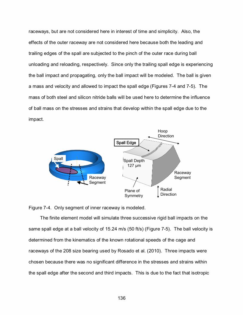
136
raceways, but are not considered here in interest of time and simplicity. Also, the
effects of the outer raceway are not considered here because both the leading and
trailing edges of the spall are subjected to the pinch of the outer race during ball
unloading and reloading, respectively. Since only the trailing spall edge is experiencing
the ball impact and propagating, only the ball impact will be modeled. The ball is given
a mass and velocity and allowed to impact the spall edge (Figures 7-4 and 7-5). The
mass of both steel and silicon nitride balls will be used here to determine the influence
of ball mass on the stresses and strains that develop within the spall edge due to the
impact.
Raceway Segment
Spall
Raceway Segment
Spall
Plane of Symmetry
Hoop Direction
Radial Direction
Spall EdgeSpall Edge
Raceway Segment
Spall Depth 127 µm
Figure 7-4. Only segment of inner raceway is modeled.
The finite element model will simulate three successive rigid ball impacts on the
same spall edge at a ball velocity of 15.24 m/s (50 ft/s) (Figure 7-5). The ball velocity is
determined from the kinematics of the known rotational speeds of the cage and
raceways of the 208 size bearing used by Rosado et al. (2010). Three impacts were
chosen because there was no significant difference in the stresses and strains within
the spall edge after the second and third impacts. This is due to the fact that isotropic
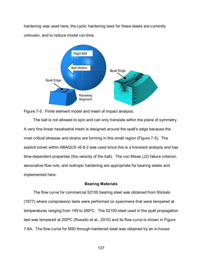
137
hardening was used here, the cyclic hardening laws for these steels are currently
unknown, and to reduce model run-time.
Spall EdgeSpall Edge
Rigid Ball
Raceway Segment
Spall Edge
Ball Motion
Rigid Ball
Raceway Segment
Spall Edge
Ball MotionBall Motion
Figure 7-5. Finite element model and mesh of impact analysis.
The ball is not allowed to spin and can only translate within the plane of symmetry.
A very fine linear hexahedral mesh is designed around the spall’s edge because the
most critical stresses and strains are forming in this small region (Figure 7-5). The
explicit solver within ABAQUS v6.8-2 was used since this is a transient analysis and has
time-dependent properties (the velocity of the ball). The von Mises (J2) failure criterion,
associative flow rule, and isotropic hardening are appropriate for bearing steels and
implemented here.
Bearing Materials
The flow curve for commercial 52100 bearing steel was obtained from Stickels
(1977) where compression tests were performed on specimens that were tempered at
temperatures ranging from 149 to 260ºC. The 52100 steel used in the spall propagation
test was tempered at 200ºC (Rosado et al., 2010) and its flow curve is shown in Figure
7-6A. The flow curve for M50 through-hardened steel was obtained by an in-house
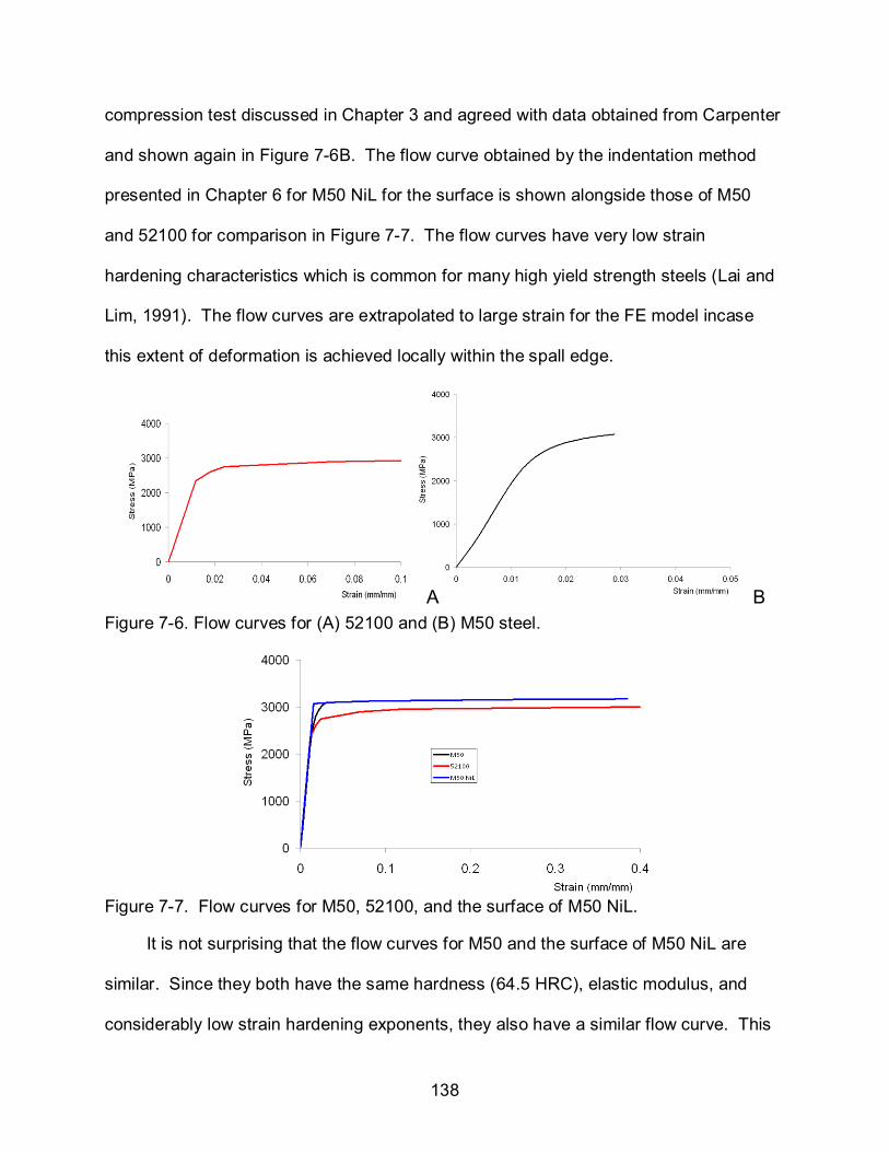
138
compression test discussed in Chapter 3 and agreed with data obtained from Carpenter
and shown again in Figure 7-6B. The flow curve obtained by the indentation method
presented in Chapter 6 for M50 NiL for the surface is shown alongside those of M50
and 52100 for comparison in Figure 7-7. The flow curves have very low strain
hardening characteristics which is common for many high yield strength steels (Lai and
Lim, 1991). The flow curves are extrapolated to large strain for the FE model incase
this extent of deformation is achieved locally within the spall edge.
A B Figure 7-6. Flow curves for (A) 52100 and (B) M50 steel.
Figure 7-7. Flow curves for M50, 52100, and the surface of M50 NiL.
It is not surprising that the flow curves for M50 and the surface of M50 NiL are
similar. Since they both have the same hardness (64.5 HRC), elastic modulus, and
considerably low strain hardening exponents, they also have a similar flow curve. This
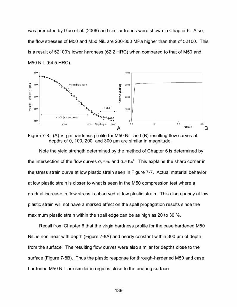
139
was predicted by Gao et al. (2006) and similar trends were shown in Chapter 6. Also,
the flow stresses of M50 and M50 NiL are 200-300 MPa higher than that of 52100. This
is a result of 52100’s lower hardness (62.2 HRC) when compared to that of M50 and
M50 NiL (64.5 HRC).
Figure 7-8. (A) Virgin hardness profile for M50 NiL and (B) resulting flow curves at
depths of 0, 100, 200, and 300 µm are similar in magnitude.
Note the yield strength determined by the method of Chapter 6 is determined by
the intersection of the flow curves σy=Eε and σy=Kεn. This explains the sharp corner in
the stress strain curve at low plastic strain seen in Figure 7-7. Actual material behavior
at low plastic strain is closer to what is seen in the M50 compression test where a
gradual increase in flow stress is observed at low plastic strain. This discrepancy at low
plastic strain will not have a marked effect on the spall propagation results since the
maximum plastic strain within the spall edge can be as high as 20 to 30 %.
Recall from Chapter 6 that the virgin hardness profile for the case hardened M50
NiL is nonlinear with depth (Figure 7-8A) and nearly constant within 300 µm of depth
from the surface. The resulting flow curves were also similar for depths close to the
surface (Figure 7-8B). Thus the plastic response for through-hardened M50 and case
hardened M50 NiL are similar in regions close to the bearing surface.

140
Residual Stress Profile M50 NiL
Residual hoop stress profiles obtained from X-Ray Diffraction (XRD) methods and
presented in Forster et al. (2010) are shown in Figure 7-9A for the virgin bearing steels
used in this study.
(a)
(b)
A
B
Figure 7-9. (A) Residual hoop stress profile for 52100, M50, and M50 NiL prior to bearing operation. (B) Residual hoop stress profile for M50 NiL next to spall edge and 120 degrees from M50 NiL spall (Forster et al., 2010).
Considerably large residual compressive stresses are present at the immediate
surface which is due to the final finishing of the bearing, but drop off substantially over a

141
depth of 10 µm. There is an initial compressive residual hoop stress profile due to the
case-hardening of the M50 NiL bearing steel that is a nearly constant 400 MPa up to a
depth of 1 mm. XRD was also performed in close proximity to the spall edge and 120
degrees from the spall edge for a spalled bearing as shown in Figure 7-9B. Note the
compressive residual stress is still present in proximity of the spall edge. The irradiated
area was on the order of 1 x 1 mm and considerably larger than the resolution needed
to compare to the residual stress profiles obtained from finite element models shown
next.
Finite Element Model of Initial Residual Hoop Stress
This initial residual compressive hoop stress of 400 MPa must be taken into
account in the FE model of the ball-spall edge impact analysis of M50 NiL. The effects
of residual hoop stress are believed to retard crack formation and spall propagation
(Forster et al., 2010) and is expected to affect the calculation of plastic strain within the
impacted spall edge in the FE model. The residual stresses within the FE model can be
applied many different ways, but in this analysis an external elastic displacement is
applied at either end of the raceway segment to induce the desired compressive hoop
stress of 400 MPa. This is similar to applying a temperature and coefficient of thermal
expansion to the segment while it is constrained at either end. In that case the segment
is allowed to expand a certain amount and then elastically compressed to the desired
stress state. Figure 7-10 shows the initial residual hoop stress state of the FE model
prior to ball impact.
Note the residual stress is a compressive 400 MPa throughout the raceway
segment with the exception of the immediate spall edge. At the free surface of the spall
edge, the residual stresses drop to -70 MPa at the location where initial ball contact

142
occurs. Boundary conditions cannot be applied to the spall edge in order to induce more
compressive stress because this is the same location as the ball impact.
350
310270 230
195 155 11070
127 µm
Hoop Direction
Figure 7-10. Compressive residual hoop stress state within raceway segment prior to ball impact.
The compressive residual stress of 400 MPa is present just below the spall edge
at a depth of 127 µm. This is likely to occur in the actual spalled bearing but cannot be
verified by XRD because the spot size of 1 x 1 mm is too large to detect this lack of
residual stress on the immediate spall edge where the actual cracks are forming. The
fact that the residual compressive stresses are so low at the spall edge may not affect
the formation of plastic strain within this region when compared to a spall edge with zero
initial compressive stress. The effects may become more obvious in the calculation of
plastic zone depth, which as seen in Chapter 3, can exceed 250 µm.
RESULTS
M50
The results of the ball impact analysis for M50 through-hardened steel from
Chapter 3 are repeated here for convenience in order to compare with the results
obtained for 52100 and M50 NiL bearing steels shown afterwards. The mass of silicon
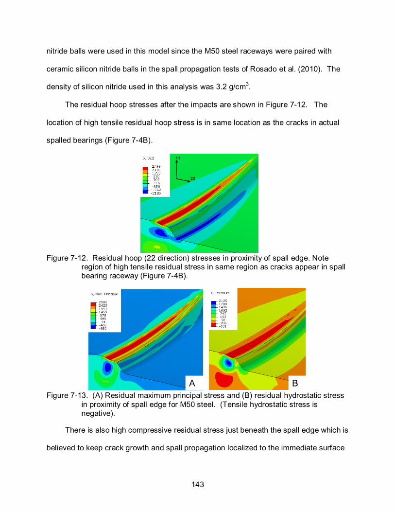
143
nitride balls were used in this model since the M50 steel raceways were paired with
ceramic silicon nitride balls in the spall propagation tests of Rosado et al. (2010). The
density of silicon nitride used in this analysis was 3.2 g/cm3.
The residual hoop stresses after the impacts are shown in Figure 7-12. The
location of high tensile residual hoop stress is in same location as the cracks in actual
spalled bearings (Figure 7-4B).
11
22
11
22
Figure 7-12. Residual hoop (22 direction) stresses in proximity of spall edge. Note
region of high tensile residual stress in same region as cracks appear in spall bearing raceway (Figure 7-4B).
A B Figure 7-13. (A) Residual maximum principal stress and (B) residual hydrostatic stress
in proximity of spall edge for M50 steel. (Tensile hydrostatic stress is negative).
There is also high compressive residual stress just beneath the spall edge which is
believed to keep crack growth and spall propagation localized to the immediate surface

144
as seen in the experiments. The residual maximum principal stress and residual
hydrostatic stress profiles are shown in Figure 7-13A and Figure 7-13B, respectively.
Note the similarity in the locations of residual tensile and compressive stress within the
impacted spall edge. Research conducted by Howell et al. (2004) has shown that
fatigue cracks are likely to initiate in regions of large hydrostatic tensile stress and
agrees with the locations of cracks in the spalled bearings.
The strain-life approaches summarized in (Suresh, 2004), such as Coffin-Manson
shown below, determine that the number of stress cycles required to initiate a crack
decreases with increasing plastic strain:
''(2 ) (2 )
2 2 2p f b ce
f f fN NE
ε σεε ε∆∆∆
= + = + (7-1)
where the total strain amplitude Δε is the sum total of the elastic Δεe and plastic Δεp
strain amplitudes. A detailed quantitative fatigue life analysis cannot be made here
since the cyclic strain-life data (such as the constants b and c) for these bearing steels
is scarce, the plastic strains calculated by the FE model are for a spall that only suffered
three impacts, and the cyclic plastic strain amplitudes from the FE model are highly
dependent on its cyclic strain hardening law which is also limited for bearing steels. As
a qualitative investigation, however, it is worth comparing the distribution of plastic strain
within the spall edge with the location of cracks in the actual bearings to see if cracks
form in the most damaged region as predicted by the FE model.
The distribution of maximum principal plastic strain is shown in Figure 7-14. The
plastic zone size is 250 µm in depth and 315 µm in width and defined by the 0.2 %
plastic strain contour. The maximum plastic strain is 0.206 and occurs in the center of
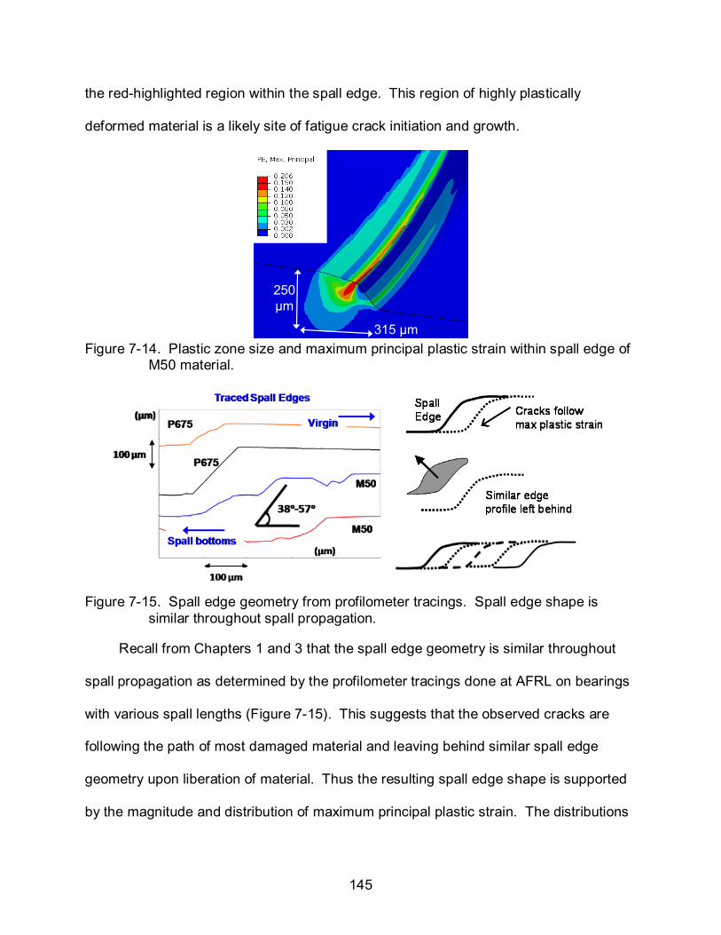
145
the red-highlighted region within the spall edge. This region of highly plastically
deformed material is a likely site of fatigue crack initiation and growth.
315 µm
250 µm
315 µm
250 µm
Figure 7-14. Plastic zone size and maximum principal plastic strain within spall edge of
M50 material.
Figure 7-15. Spall edge geometry from profilometer tracings. Spall edge shape is
similar throughout spall propagation.
Recall from Chapters 1 and 3 that the spall edge geometry is similar throughout
spall propagation as determined by the profilometer tracings done at AFRL on bearings
with various spall lengths (Figure 7-15). This suggests that the observed cracks are
following the path of most damaged material and leaving behind similar spall edge
geometry upon liberation of material. Thus the resulting spall edge shape is supported
by the magnitude and distribution of maximum principal plastic strain. The distributions
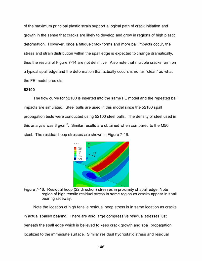
146
of the maximum principal plastic strain support a logical path of crack initiation and
growth in the sense that cracks are likely to develop and grow in regions of high plastic
deformation. However, once a fatigue crack forms and more ball impacts occur, the
stress and strain distribution within the spall edge is expected to change dramatically,
thus the results of Figure 7-14 are not definitive. Also note that multiple cracks form on
a typical spall edge and the deformation that actually occurs is not as “clean” as what
the FE model predicts.
52100
The flow curve for 52100 is inserted into the same FE model and the repeated ball
impacts are simulated. Steel balls are used in this model since the 52100 spall
propagation tests were conducted using 52100 steel balls. The density of steel used in
this analysis was 8 g/cm3. Similar results are obtained when compared to the M50
steel. The residual hoop stresses are shown in Figure 7-16.
11
22
Figure 7-16. Residual hoop (22 direction) stresses in proximity of spall edge. Note
region of high tensile residual stress in same region as cracks appear in spall bearing raceway.
Note the location of high tensile residual hoop stress is in same location as cracks
in actual spalled bearing. There are also large compressive residual stresses just
beneath the spall edge which is believed to keep crack growth and spall propagation
localized to the immediate surface. Similar residual hydrostatic stress and residual

147
maximum principal stress profiles are shown in Figure 7-17A and Figure 7-17B,
respectively.
A B Figure 7-17. (A) Residual hydrostatic stress and (B) residual maximum principal stress
in proximity of spall edge for 52100 steel.
500 µm
460 µm
Figure 7-18. Plastic zone size and maximum principal plastic strain magnitude within
spall edge of 52100 steel.
The distribution of maximum principal plastic strain is shown in Figure 7-18. The
plastic zone size is 460 µm in depth and 500 µm in width which is 84 % deeper and 58
% wider than the M50 test case. The maximum plastic strain is 0.265 and 32 % higher
than M50 (0.20). From these results it cannot be determined if the larger amount of
plastic deformation is due to the heavier ball mass or lower hardness, but the
contributions from each will be determined in a later section. The fact that 52100
exhibits greater plastic strains where cracks are forming and a larger volume of

148
plastically deformed material is indicative of the faster spall propagation rates seen in
Rosado et al. (2010) and earlier in this chapter. Many fatigue failure theories such as
Coffin-Manson predict cracks to form sooner in regions of greater plastic strain (Suresh,
2004) which supports the faster spall propagation behavior of 52100.
M50 NiL
The flow curve variation for M50 NiL that was determined in Chapter 6 is inserted
into the same FE model and the repeated ball impacts are simulated using ceramic
silicon nitride balls. There is also an initial compressive stress of 400 MPa within the
raceway segment as discussed earlier in this chapter. Similar residual stress profiles
around the spall edge after ball impacts are obtained when compared to the M50 test
cases. The residual hoop stresses are shown in Figure 7-19.
11
22
Figure 7-19. Residual hoop (22 direction) stress in proximity of spall edge of M50 NiL. Note region of high tensile residual stress in same region as cracks appear in spall bearing raceway.
Note the location of high tensile residual hoop stress is in same location as cracks
in actual spalled bearing and the high compressive residual stress just beneath the spall
edge. The residual hydrostatic stress and residual maximum principal stress profiles
are shown in Figure 7-20A and Figure 7-20B, respectively. Once again there is
similarity in the locations of residual tensile and compressive stress within the impacted
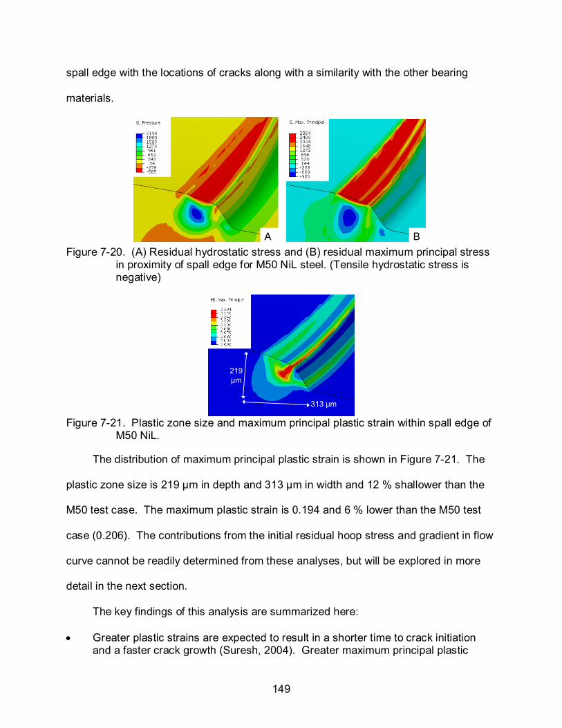
149
spall edge with the locations of cracks along with a similarity with the other bearing
materials.
A B Figure 7-20. (A) Residual hydrostatic stress and (B) residual maximum principal stress
in proximity of spall edge for M50 NiL steel. (Tensile hydrostatic stress is negative)
313 µm
219 µm
Figure 7-21. Plastic zone size and maximum principal plastic strain within spall edge of
M50 NiL.
The distribution of maximum principal plastic strain is shown in Figure 7-21. The
plastic zone size is 219 µm in depth and 313 µm in width and 12 % shallower than the
M50 test case. The maximum plastic strain is 0.194 and 6 % lower than the M50 test
case (0.206). The contributions from the initial residual hoop stress and gradient in flow
curve cannot be readily determined from these analyses, but will be explored in more
detail in the next section.
The key findings of this analysis are summarized here:
• Greater plastic strains are expected to result in a shorter time to crack initiation and a faster crack growth (Suresh, 2004). Greater maximum principal plastic

150
strains were determined for 52100 when compared to the lesser values for M50 and M50 NiL. This is indicative of the faster propagation rates observed for 52100 in all spall propagation tests.
• This observed behavior for 52100 is thought to be caused by the combined effects of the heavier ball mass (steel vs silicon nitride balls) and its lower hardness, yield strength, and flow curve inherent to 52100 bearing steel.
• The spall edge of 52100 also displayed a larger plastic zone when compared to M50 and M50 NiL. Thus more material points are experiencing cyclic plasticity, which increases the probability of crack initiation to occur in a shorter amount of time. This was observed experimentally in the faster spall propagation tests of 52100.
• Similar results in plastic strains and residual stresses were obtained for M50 NiL and M50 which agrees with the comparable spall propagation behavior observed in the spall propagation tests.
• The plastic zone depth was 30 µm deeper for the M50 test case when compared to that of M50 NiL. This may be indicative of the compressive residual stress or gradient in flow curve in M50 NiL that may prevent the plastic zone from developing in deeper regions.
• Once a crack forms and balls continue to impact the spall edge, the stress and plastic strain distribution will change dramatically. Thus the results presented here are not comprehensive.
• Although the findings from this FE analysis are supportive of what is observed experimentally, the contributions from ball mass, initial residual stress, surface hardness, and gradient in flow curve cannot be deduced from this limited set of data. The next section will investigate the contributions from each by only changing one variable at a time.
Effects of Individual Contributions
Residual Stress
The spall edge impact model will be repeated for various preconditions in order to
determine the contributions from initial residual stress, gradient in flow curve, ball mass,
and surface hardness. The M50 NiL test case included an initial residual compressive
hoop stress of 400 MPa prior to the ball impacts. From the previous results, it was
uncertain how this residual stress affected the formation and severity of the plastic
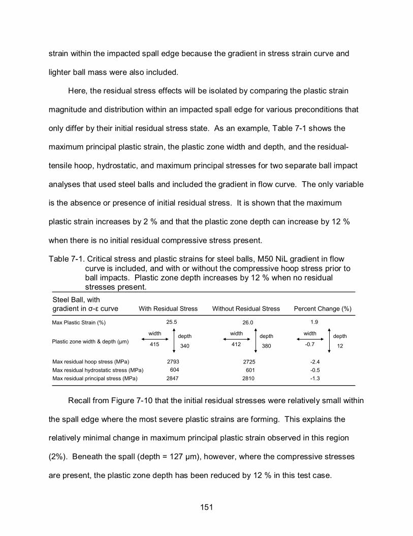
151
strain within the impacted spall edge because the gradient in stress strain curve and
lighter ball mass were also included.
Here, the residual stress effects will be isolated by comparing the plastic strain
magnitude and distribution within an impacted spall edge for various preconditions that
only differ by their initial residual stress state. As an example, Table 7-1 shows the
maximum principal plastic strain, the plastic zone width and depth, and the residual-
tensile hoop, hydrostatic, and maximum principal stresses for two separate ball impact
analyses that used steel balls and included the gradient in flow curve. The only variable
is the absence or presence of initial residual stress. It is shown that the maximum
plastic strain increases by 2 % and that the plastic zone depth can increase by 12 %
when there is no initial residual compressive stress present.
Table 7-1. Critical stress and plastic strains for steel balls, M50 NiL gradient in flow curve is included, and with or without the compressive hoop stress prior to ball impacts. Plastic zone depth increases by 12 % when no residual stresses present.
Steel Ball, with gradient in σ-ε curve With Residual Stress Without Residual Stress
Max Plastic Strain (%)
Plastic zone width & depth (µm)
25.5 26.0
width depth
340415
width depth
380412
Percent Change (%)
1.9
width depth
12-0.7
Max residual hoop stress (MPa)Max residual hydrostatic stress (MPa) 604 601
2793 2725 -2.4-0.5
Max residual principal stress (MPa) 2847 2810 -1.3
Recall from Figure 7-10 that the initial residual stresses were relatively small within
the spall edge where the most severe plastic strains are forming. This explains the
relatively minimal change in maximum principal plastic strain observed in this region
(2%). Beneath the spall (depth = 127 µm), however, where the compressive stresses
are present, the plastic zone depth has been reduced by 12 % in this test case.
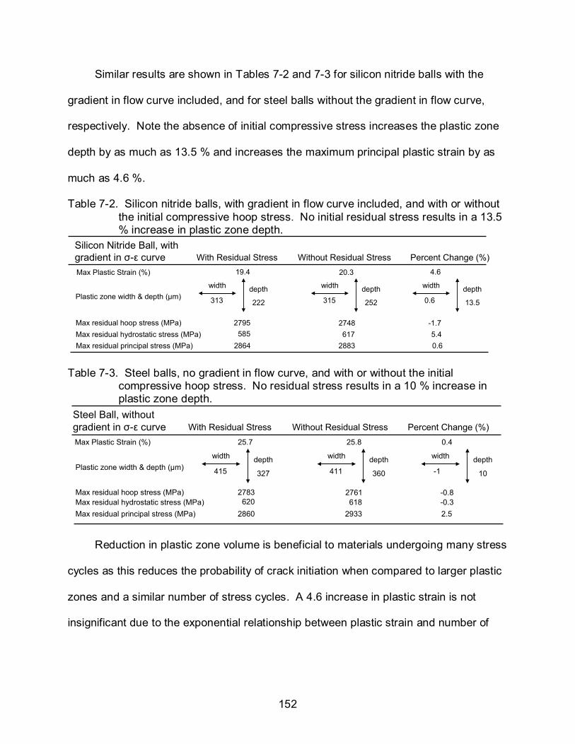
152
Similar results are shown in Tables 7-2 and 7-3 for silicon nitride balls with the
gradient in flow curve included, and for steel balls without the gradient in flow curve,
respectively. Note the absence of initial compressive stress increases the plastic zone
depth by as much as 13.5 % and increases the maximum principal plastic strain by as
much as 4.6 %.
Table 7-2. Silicon nitride balls, with gradient in flow curve included, and with or without the initial compressive hoop stress. No initial residual stress results in a 13.5 % increase in plastic zone depth.
Silicon Nitride Ball, with gradient in σ-ε curve With Residual Stress Without Residual StressMax Plastic Strain (%)
Plastic zone width & depth (µm)
19.4 20.3
width depth
222313
width depth
252315
Percent Change (%)4.6
width depth
13.50.6
Max residual hoop stress (MPa)Max residual hydrostatic stress (MPa) 585 617
2795 2748 -1.75.4
Max residual principal stress (MPa) 2864 2883 0.6 Table 7-3. Steel balls, no gradient in flow curve, and with or without the initial
compressive hoop stress. No residual stress results in a 10 % increase in plastic zone depth.
Steel Ball, without gradient in σ-ε curve With Residual Stress Without Residual StressMax Plastic Strain (%)
Plastic zone width & depth (µm)
25.7 25.8
width depth
327415
width depth
360411
Percent Change (%)0.4
width depth
10-1
Max residual hoop stress (MPa)Max residual hydrostatic stress (MPa) 620 618
2783 2761 -0.8-0.3
Max residual principal stress (MPa) 2860 2933 2.5
Reduction in plastic zone volume is beneficial to materials undergoing many stress
cycles as this reduces the probability of crack initiation when compared to larger plastic
zones and a similar number of stress cycles. A 4.6 increase in plastic strain is not
insignificant due to the exponential relationship between plastic strain and number of

153
cycles to crack initiation, but may not have as big of an influence as ball mass or
surface hardness as will be shown later.
The residual maximum hoop, hydrostatic, and maximum principal stresses were
too close in magnitude to report any significance. Due to the amount of data presented
in the following tables the contour plots of the residual plastic strain and stresses will not
be shown.
It is well known that initial residual compressive hoop stresses increase the fatigue
life of rolling element bearings prior to fatigue spall formation (Forster et al., 2010).
However, it was observed in the spall propagation experiments of Figure 7-1 where a
few, but not all of the M50 specimens (no initial residual compressive stress) lasted
longer than the M50 NiL specimens (initial residual compressive stress was present).
This may be due to the combination of lower fracture toughness of the case hardened
M50 NiL and compressive residual stresses, which together, yield similar propagation
characteristics as M50 which has higher fracture toughness, but no compressive
stresses.
Gradient in Stress-Strain Curve
The contributions from the gradient in stress-strain (flow) curve will now be
considered. The through-hardened M50 bearing steel has a constant hardness
throughout (64.5 HRC). The M50 NiL steel has a nonlinear decreasing gradient in
hardness as seen visually in Figure 7-8A, but a similar surface hardness of 64.5 HRC
(820Hv) as M50. From the results at the beginning of this chapter it was unclear how
the gradient in flow curve affected the magnitude or distribution of plastic strain within
the spall edge. It was shown in Figure 7-8A that the hardness is similar within the first
300 µm of depth and the corresponding flow curve variation was also minimal in this

154
region (Figure 7-8B). This causes similarities in the plastically deformed region of the
impacted spall edge as shown in Tables 7-4 and 7-5 where the spall edge impact model
is repeated for steel balls with and without residual stress, respectively.
Table 7-4. Effects of gradient in flow curve using steel balls and initial residual stresses are present. Plastic zone depth is only slightly deeper when gradient in flow curve is included.
Steel Ball, with Residual Stress
With Gradient in σ-ε curve
Max Plastic Strain (%)
Plastic zone width & depth (µm)
25.5width depth
340415
Percent Change (%)
0.7width depth
-40.0
Max residual hoop stress (MPa)Max residual hydrostatic stress (MPa) 604
2793 -0.42.6
Max residual principal stress (MPa) 2847 0.4
Without Gradient in σ-ε curve
25.7width depth
327415
6202783
2860
Here, only the gradient in flow curve is present or not for each case with all other
contributions kept as constants for comparison. Results with and without the gradient in
flow curve are shown in both Tables 7-4 and 7-5. Interestingly, the plastic zone is
slightly deeper when there is a gradient in flow curve (Table 7-4), and also occurs when
there are no residual compressive stresses present (Table 7-5). This is intuitive since
the yield strength is decreasing with depth, so will the resistance to plastic deformation
and consequently deeper plastic zones will develop. The maximum principal plastic
strain within the spall edge is similar in magnitude (0.7%) for these cases because the
gradient in yield strength is minimal within its shallow depth (127 µm).
These results suggest that the gradient in hardness does not reduce the severity
of spall propagation and supports what was shown in Figures 7-1 and 7-2 where M50
NiL did not outperform M50 in the spall propagation tests. It is well known that M50 NiL
exhibits a longer rolling contact fatigue than M50 prior to spall initiation (Forster et al.,
2010) due to the gradient in hardness and presence of residual compressive stress, but

155
these effects do not appear to reduce spall propagation as seen here and in the
experiments.
Table 7-5. Effects of gradient in flow curve using steel balls without initial residual stress present. Plastic zone depth is 10 % deeper when gradient in flow curve is not included.
Steel Ball, without Residual Stress
Max Plastic Strain (%)
Plastic zone width & depth (µm)
25.8
width depth
360411
Percent Change (%)
-0.8
width depth
-5.3-0.2
Max residual hoop stress (MPa)
Max residual hydrostatic stress (MPa) 618
2761 0.8
0.3Max residual principal stress (MPa) 2933 2.5
With Gradient in σ-ε curve
Without Gradient in σ-ε curve
26.0
width depth
380412
601
2725
2810
Surface Hardness
The effect of surface hardness on the extent of plastic deformation is now
considered using steel balls with all other variables held constant. The results from the
52100 impact analysis are compared to M50 because the effects of residual stress and
gradient in stress strain curve were not present in the 52100 and M50 bearing steels.
Even though the M50 raceway was paired with ceramic silicon nitride balls in the actual
spall-propagation experiments, this analysis will impact the M50 spall edge with steel
balls to remove any discrepancy in ball mass. The effects of ball mass will be
determined later in the next section, but for now only the effects of surface hardness
(flow curve) will be considered.
As was shown in Figure 7-6 the M50 steel has a higher flow stress than 52100 by
200-300 MPa for a large range in plastic strain. The softer 52100 is then expected to
experience more plastic deformation and this is observed in Table 7-6 where the plastic
strain magnitude and size is shown for these two test cases. The 52100 exhibited
nearly 3 % higher plastic strain in the region where cracks are observed to occur in

156
actual spall edges. Also the plastic zone was 22 % deeper and 18 % wider for 52100
when compared to M50. The effect of surface hardness has a larger impact on plastic
deformation than initial residual stress or gradient in flow curve. These results support
the spall propagation trends of Figures 7-1 and 7-2 in the sense that larger magnitudes
and volumes of plastic deformation result in a reduction of the number of stress cycles
to crack initiation and spall growth.
Table 7-6. Effects of surface hardness using steel balls, no initial residual stress, and no gradient in flow curve. Lower surface hardness results in larger plastic zones.
Effect of surface hardness, 52100 (62.2 HRC) and M50/M50NiL (64.5 HRC) 52100
Max Plastic Strain (%)
Plastic zone width & depth (µm)
Percent Change (%)
-2.7
width depth
-22-18
Max residual hoop stress (MPa)Max residual hydrostatic stress (MPa)
1827
Max residual principal stress (MPa) 16
Without Residual Stress, Without Gradient in σ-ε curve
26.5
width depth
460500
4842338
2518
25.8
width depth
360411
6182761
2933
Interestingly the M50 showed higher tensile residual hoop, hydrostatic, and
maximum principal stress. This is due to the fact that the M50 can strain harden to
higher flow stresses during plastic deformation and also has a similar elastic rebound
(elastic modulus) as 52100. It is plausible that the magnitude of tensile residual stress
as calculated by this method is not indicative of fatigue crack initiation in the sense that
M50 displayed better spall propagation characteristics than 52100.
Ball Mass
Ceramic silicon nitride balls are being increasingly used in high performance
bearings due to their high hardness, low density, and performance in oil-out conditions.
Bearings that use ceramic balls have shown better spall propagation characteristics
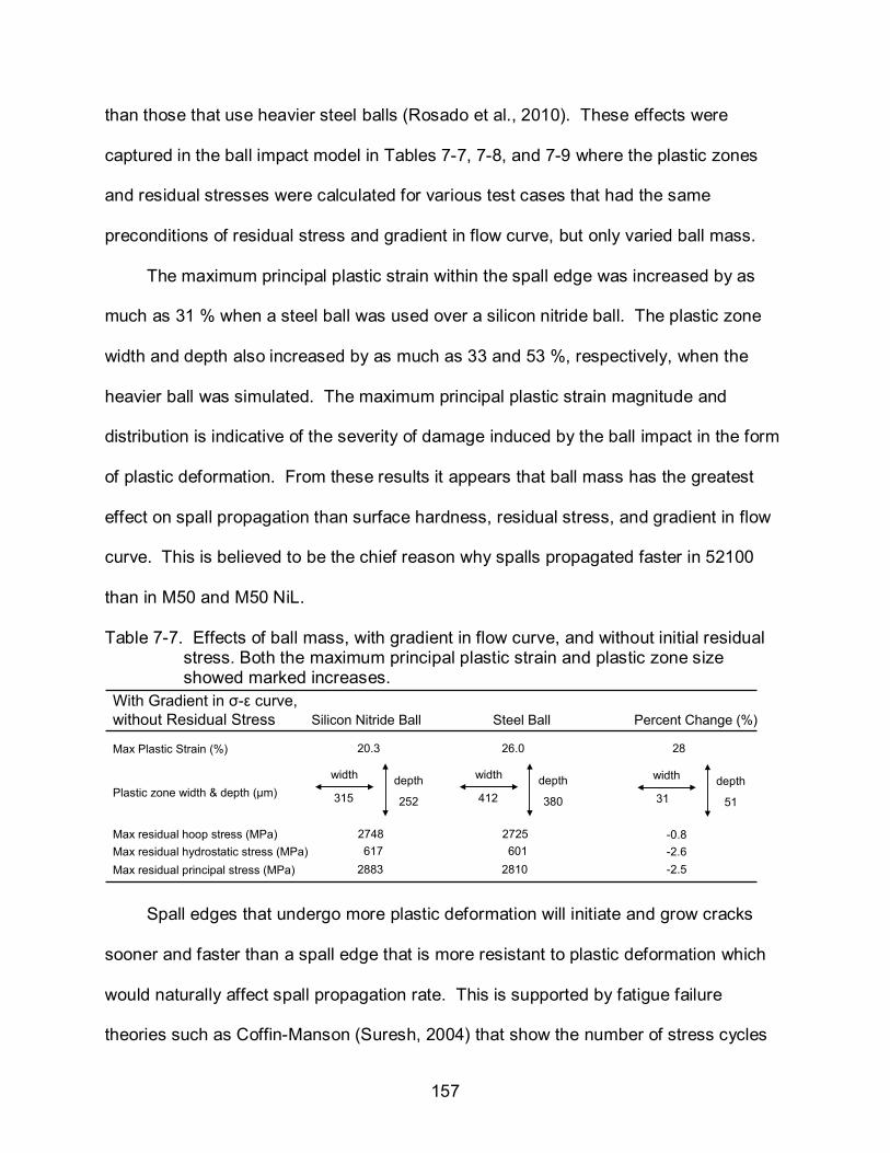
157
than those that use heavier steel balls (Rosado et al., 2010). These effects were
captured in the ball impact model in Tables 7-7, 7-8, and 7-9 where the plastic zones
and residual stresses were calculated for various test cases that had the same
preconditions of residual stress and gradient in flow curve, but only varied ball mass.
The maximum principal plastic strain within the spall edge was increased by as
much as 31 % when a steel ball was used over a silicon nitride ball. The plastic zone
width and depth also increased by as much as 33 and 53 %, respectively, when the
heavier ball was simulated. The maximum principal plastic strain magnitude and
distribution is indicative of the severity of damage induced by the ball impact in the form
of plastic deformation. From these results it appears that ball mass has the greatest
effect on spall propagation than surface hardness, residual stress, and gradient in flow
curve. This is believed to be the chief reason why spalls propagated faster in 52100
than in M50 and M50 NiL.
Table 7-7. Effects of ball mass, with gradient in flow curve, and without initial residual stress. Both the maximum principal plastic strain and plastic zone size showed marked increases.
With Gradient in σ-ε curve, without Residual Stress Silicon Nitride Ball
Max Plastic Strain (%)
Plastic zone width & depth (µm)
Percent Change (%)
28
width depth
5131
Max residual hoop stress (MPa)Max residual hydrostatic stress (MPa)
-0.8-2.6
Max residual principal stress (MPa) -2.5
Steel Ball
20.3
width depth
252315
6172748
2883
26.0
width depth
380412
6012725
2810
Spall edges that undergo more plastic deformation will initiate and grow cracks
sooner and faster than a spall edge that is more resistant to plastic deformation which
would naturally affect spall propagation rate. This is supported by fatigue failure
theories such as Coffin-Manson (Suresh, 2004) that show the number of stress cycles
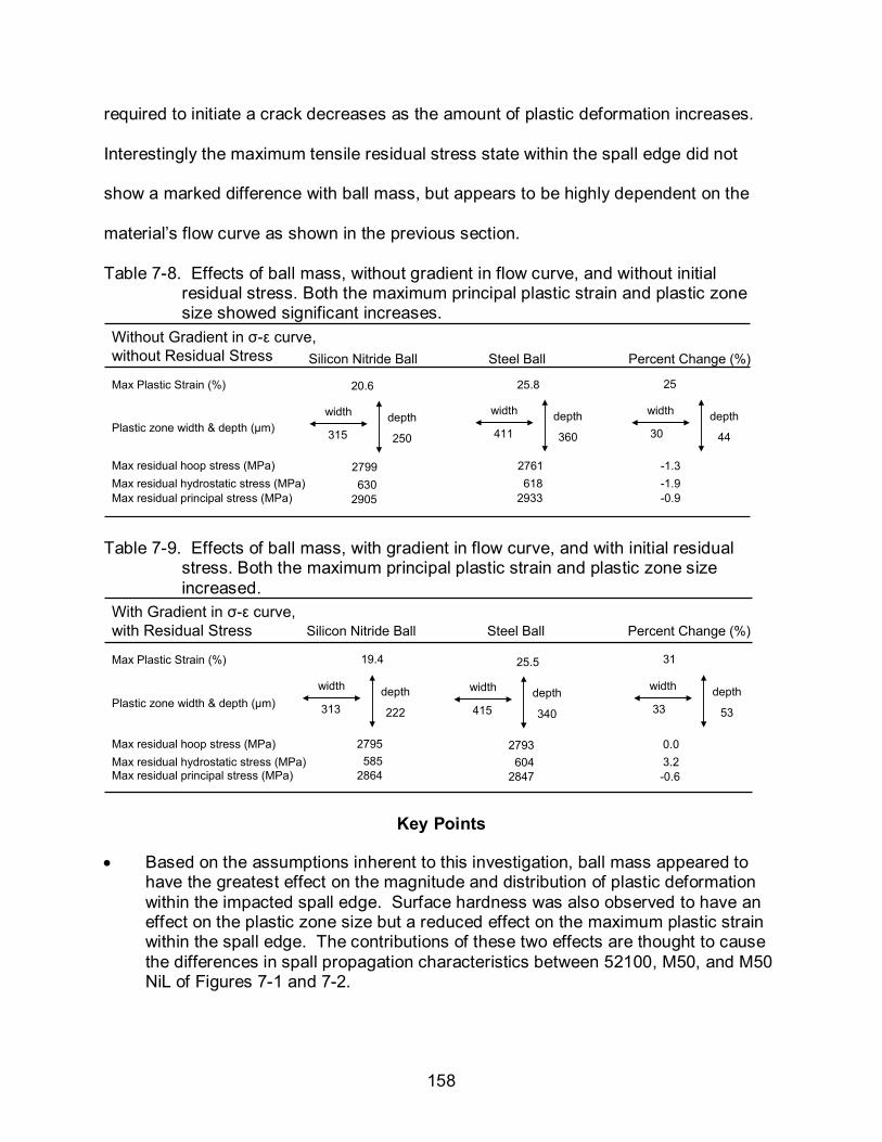
158
required to initiate a crack decreases as the amount of plastic deformation increases.
Interestingly the maximum tensile residual stress state within the spall edge did not
show a marked difference with ball mass, but appears to be highly dependent on the
material’s flow curve as shown in the previous section.
Table 7-8. Effects of ball mass, without gradient in flow curve, and without initial residual stress. Both the maximum principal plastic strain and plastic zone size showed significant increases.
Without Gradient in σ-ε curve, without Residual Stress Silicon Nitride Ball
Max Plastic Strain (%)
Plastic zone width & depth (µm)
Percent Change (%)
25
width depth
4430
Max residual hoop stress (MPa)Max residual hydrostatic stress (MPa)
-1.3-1.9
Max residual principal stress (MPa) -0.9
Steel Ball
20.6
width depth
250315
6302799
2905
25.8
width depth
360411
6182761
2933
Table 7-9. Effects of ball mass, with gradient in flow curve, and with initial residual
stress. Both the maximum principal plastic strain and plastic zone size increased.
With Gradient in σ-ε curve, with Residual Stress Silicon Nitride Ball
Max Plastic Strain (%)
Plastic zone width & depth (µm)
Percent Change (%)
31
width depth
5333
Max residual hoop stress (MPa)Max residual hydrostatic stress (MPa)
0.03.2
Max residual principal stress (MPa) -0.6
Steel Ball
19.4
width depth
222313
5852795
2864
25.5
width depth
340415
6042793
2847
Key Points
• Based on the assumptions inherent to this investigation, ball mass appeared to have the greatest effect on the magnitude and distribution of plastic deformation within the impacted spall edge. Surface hardness was also observed to have an effect on the plastic zone size but a reduced effect on the maximum plastic strain within the spall edge. The contributions of these two effects are thought to cause the differences in spall propagation characteristics between 52100, M50, and M50 NiL of Figures 7-1 and 7-2.
159
• The effects of compressive hoop stress and gradient in flow curve were not so obvious. Significant compressive stresses did not develop within the spall edge in the region of large plastic strain because of the spall edge geometry. Thus similar results for maximum principal plastic strain were obtained. However, the plastic zone depth was decreased by the presence of compressive stress beneath the spall edge which may be beneficial to propagation, but a definitive conclusion cannot be made based on the data.
• The effects of the gradient in flow curve were not significant for M50 NiL since the variation in hardness is nearly constant within 300 µm of depth from the surface. The small variation in plastic response obtained from Chapter 6 within this region close to the surface, and explains why the plastic strain results were similar for the test cases examined. The plastic zone was actually deeper for the spall edges that had a gradient in plastic response because the reduction in yield strength with depth is more susceptible to plastic deformation and allows deeper plastic zones to develop.
Limitations
A few limitations of this analysis must be addressed here. A marked difference in
spall propagation behavior was noticed between the life-endurance tested bearings and
the virgin bearings whose spalls were initiated by Rockwell C indents. After the tens of
billions of rolling contact stress cycles experienced by the raceway’s ball track the flow
curve of a material is expected to change due to material fatigue and cyclic hardening
(or softening). This would explain the spall propagation results of the life-endurance
bearings of Figure 7-3 where 52100 outperformed the M50 steels.
However, because there were only two bearings tested of each material, definitive
conclusions cannot be made. Thus the flow curves used in this analysis are closer to
the actual plastic behavior of the virgin bearings that had their spalls initiated by indents
than naturally from billions of previous stress cycles. The FE results are supportive of
the propagation trends on the virgin raceways and not the life-endurance tested
bearings. The cyclic plastic flow behavior of M50 would need to be determined in order
to explain this phenomenon.
160
Also complex bearings dynamics exist in the actual spalled bearings during
bearing operation that are not accounted for here. Advanced software such as
Advanced Dynamics of Rolling Elements (ADORE) is currently being developed to solve
the complex problems of how a ball reloads itself between the inner and outer raceways
during spall propagation which may effect the amount of damaged experienced by a
spall edge.
The loading and boundary conditions of this FE model were relatively simple when
compared to the many complex interactions that occur between the balls, two raceways,
and bearing cage. As the spall length increases, the number of unloaded balls also
increases which causes more shaft misalignment and leads to greater contact forces on
the ball as it reestablishes contact between the raceways. As a spall propagates,
severe vibrations occur within the engine or bearing test rig that would affect the
dynamics of ball and spall edge interactions. The above mentioned complications were
not taken into account in this analysis, but may have an increased effect on the damage
induced on a spall edge.
Also the influences of fracture toughness were not accounted for in this analysis
but may have an important effect on the rate at which these spalls propagate. The
fracture toughness may also change with the large amounts of plastic deformation
experienced by the spall edge and may not be accurately represented by the method
that the fracture toughness was determined. However, this analysis is the first of its
kind in its attempt to capture the extent of damage experienced by a spall edge during
spall propagation and the contributions from residual stress, ball mass, surface
hardness, and gradient in flow curve. These contributions as determined by this

161
method were supportive of the spall propagation characteristics of 52100, M50, and
M50 NiL presented in Rosado et al. (2010).
The conclusions regarding the individual contributions from ball mass, surface
hardness, residual stress, and gradient in stress strain curve are applicable to and
supportive of the bearings used in the spall propagation experiments conducted by
AFRL and may not apply to all possible types of bearings and operating conditions. For
instance, the actual bearings used in the jet engines are much larger than the scaled
versions used in the spall propagation experiments, i.e. the engine bearings have larger
balls but similar case depths. Thus the gradient in hardness and compressive residual
stress may have a larger contribution on spall propagation than what was seen in the
smaller bearings due to the larger plastic zones that would develop for the larger balls.
Also, the effects of ball mass may diminish at lower rotational speeds than those
conducted in these experiments. In other words, the difference in ball momentum
between ceramic and steel balls will be less for lower ball velocities but significant for
high speed bearing applications.

162
CHAPTER 8 SUMMARY
Despite their optimized design, bearings cannot escape the damage induced by
foreign object debris, improper handling, overloading, or material fatigue which can
cause surface fatigue failures to occur in the form of small pits or spalls. Spalls grow
and propagate with continued engine use and allow the main engine shaft to misalign
leading to total engine failure and possibly loss of aircraft. Thus the amount of time
between initial spallation and engine failure is of great importance to pilot safety and
mission success.
Spall propagation experiments carried out by the Air Force Research Labs show
that M50, M50NiL, and 52100 bearing steels have different spall propagation
characteristics, but it is uncertain how certain aspects of bearing design such as initial
residual stress, surface hardness, gradient in flow curve, and ball mass affect spall
propagation rate. Both static and dynamic analyses were performed here to simulate
these contributions and the bearing operating conditions during spall propagation.
The material properties of case hardened M50 NiL bearing steel were initially
unknown and it was uncertain how its gradient in plastic response affected spall
propagation that occurs within this case hardened region. A new method shown here
used indentation experiments and finite element modeling to determine the plastic
response of plastically graded, P675 and M50 NiL case hardened bearing steels. The
gradient in plastic response was determined without knowing the plastic flow behavior of
the core M50 NiL region. The method utilized a material-dependent representative
plastic strain that can be used to relate indentation hardness measurements to flow
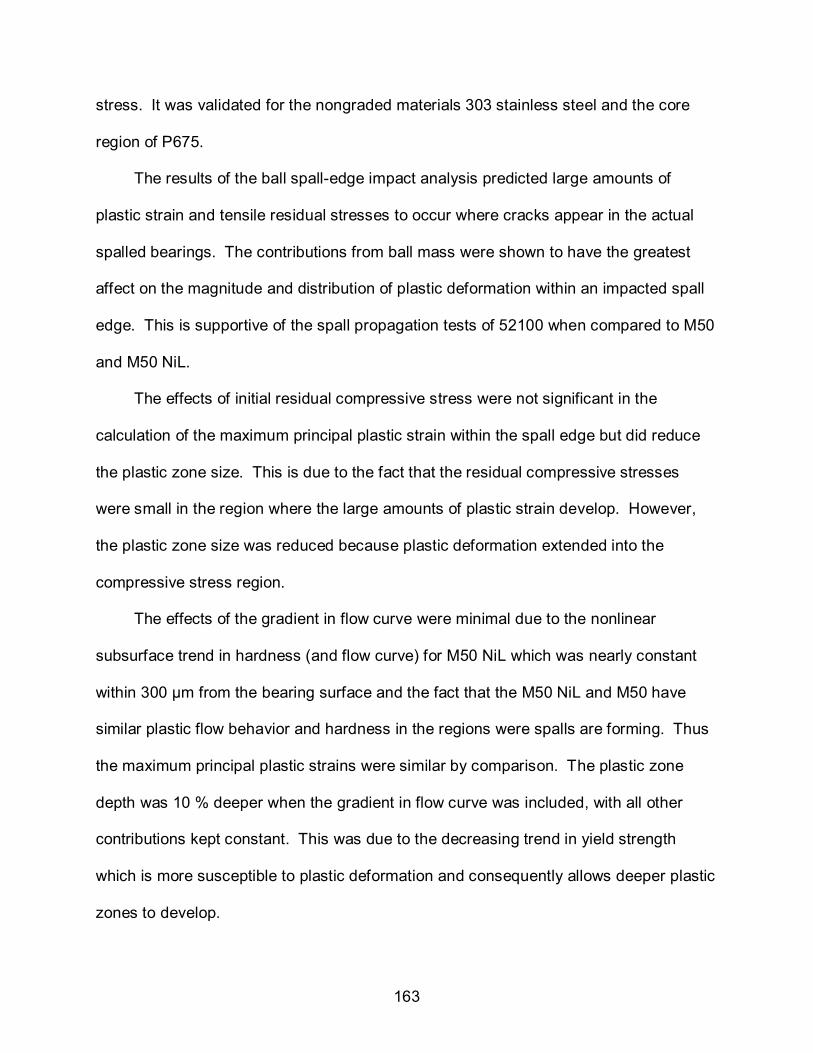
163
stress. It was validated for the nongraded materials 303 stainless steel and the core
region of P675.
The results of the ball spall-edge impact analysis predicted large amounts of
plastic strain and tensile residual stresses to occur where cracks appear in the actual
spalled bearings. The contributions from ball mass were shown to have the greatest
affect on the magnitude and distribution of plastic deformation within an impacted spall
edge. This is supportive of the spall propagation tests of 52100 when compared to M50
and M50 NiL.
The effects of initial residual compressive stress were not significant in the
calculation of the maximum principal plastic strain within the spall edge but did reduce
the plastic zone size. This is due to the fact that the residual compressive stresses
were small in the region where the large amounts of plastic strain develop. However,
the plastic zone size was reduced because plastic deformation extended into the
compressive stress region.
The effects of the gradient in flow curve were minimal due to the nonlinear
subsurface trend in hardness (and flow curve) for M50 NiL which was nearly constant
within 300 µm from the bearing surface and the fact that the M50 NiL and M50 have
similar plastic flow behavior and hardness in the regions were spalls are forming. Thus
the maximum principal plastic strains were similar by comparison. The plastic zone
depth was 10 % deeper when the gradient in flow curve was included, with all other
contributions kept constant. This was due to the decreasing trend in yield strength
which is more susceptible to plastic deformation and consequently allows deeper plastic
zones to develop.
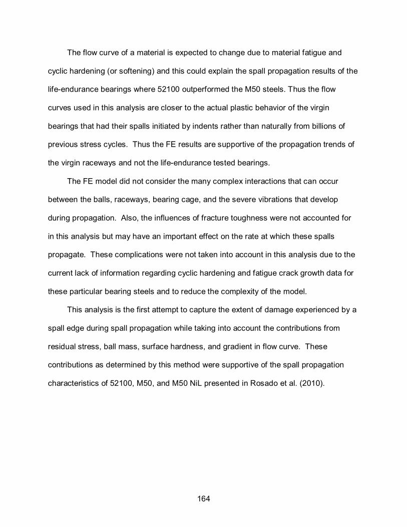
164
The flow curve of a material is expected to change due to material fatigue and
cyclic hardening (or softening) and this could explain the spall propagation results of the
life-endurance bearings where 52100 outperformed the M50 steels. Thus the flow
curves used in this analysis are closer to the actual plastic behavior of the virgin
bearings that had their spalls initiated by indents rather than naturally from billions of
previous stress cycles. Thus the FE results are supportive of the propagation trends of
the virgin raceways and not the life-endurance tested bearings.
The FE model did not consider the many complex interactions that can occur
between the balls, raceways, bearing cage, and the severe vibrations that develop
during propagation. Also, the influences of fracture toughness were not accounted for
in this analysis but may have an important effect on the rate at which these spalls
propagate. These complications were not taken into account in this analysis due to the
current lack of information regarding cyclic hardening and fatigue crack growth data for
these particular bearing steels and to reduce the complexity of the model.
This analysis is the first attempt to capture the extent of damage experienced by a
spall edge during spall propagation while taking into account the contributions from
residual stress, ball mass, surface hardness, and gradient in flow curve. These
contributions as determined by this method were supportive of the spall propagation
characteristics of 52100, M50, and M50 NiL presented in Rosado et al. (2010).

165
APPENDIX INDENTATION DATA
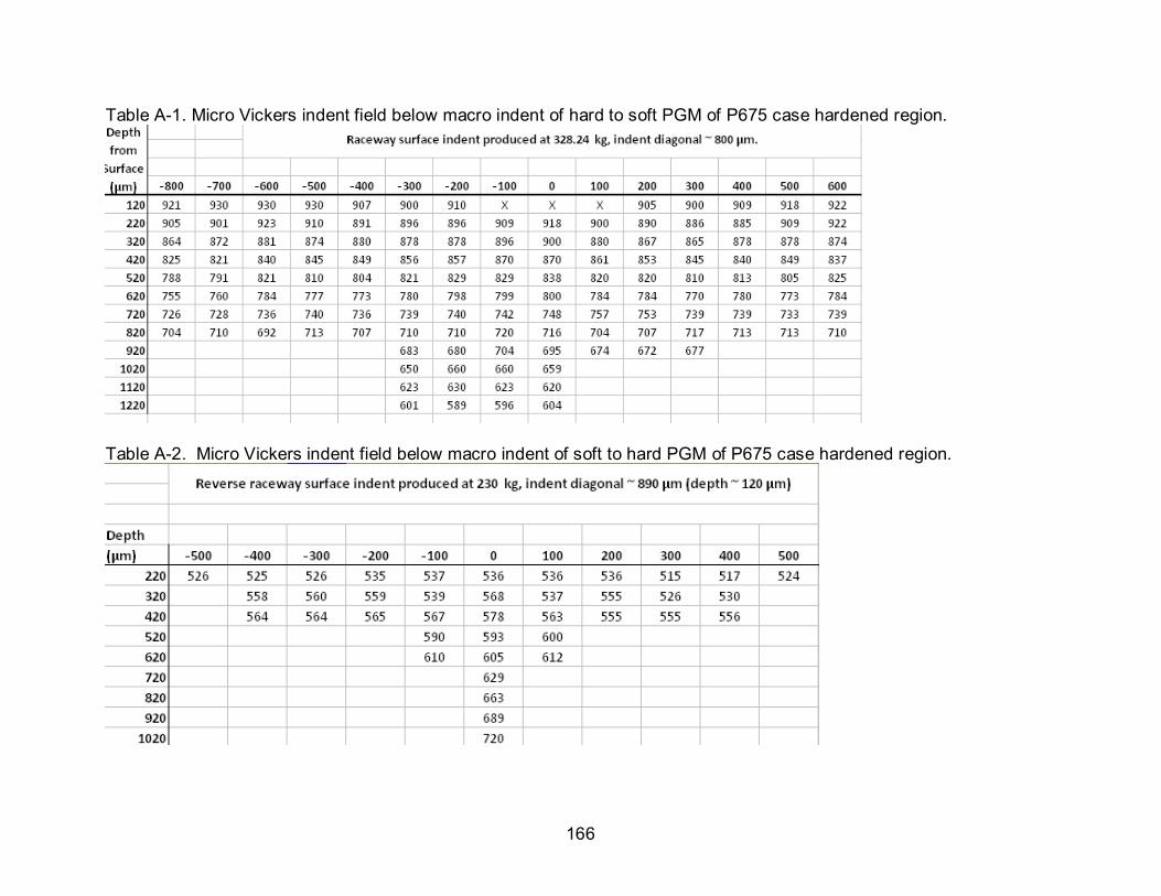
166
Table A-1. Micro Vickers indent field below macro indent of hard to soft PGM of P675 case hardened region.
Table A-2. Micro Vickers indent field below macro indent of soft to hard PGM of P675 case hardened region.

167
LIST OF REFERENCES
ASM Handbook, http://products.asminternational.org/hbk/index.jsp, June 9, 2009. Antunes J.M., Fernandes J.V., Menezes L.F., Chaparro B.M., 2007. A new approach
for reverse analyses in depth sensing indentation using numerical simulation. Acta Materialia. 55, 69-81.
Averbach, B.L., Lou, B., Pearson, P.K., Fairchild, R.E., Bamberger, E.N., 1985. Fatigue crack propagation in carburized high alloy bearing steels. Metallurgical Transactions A, 16A, 1253-1265.
Arakere, N. K., Branch, N., Levesque, G., Svendsen, V., Forster,N.H., 2010. On the Rolling Contact Fatigue Life and Spall Propagation Characteristics of M50, M50 NiL and 52100 Bearing Materials: Part II: Stress Modeling, Tribology Transactions. 53, 1, 42-51.
Baxevani E.A., Giannakopoulos A.E., 2009. The Modified Rockwell Test: A New Probe for Mechanical Properties of Metals. Experimental Mechanics. 49. 371-382.
Beswick, J.M., 1989. Fracture and fatigue crack propagation properties of hardened 52100 steel. Metallurgical Transactions A, 20A, 1961-1973.
Boresi A., Schmidt R.J., 2003. Advanced Mechanics of Materials. 6th ed. John Wiley and Sons
Branch, N.A., Arakere, N.K., Svendsen, V., Forster, N.H., 2010. Stress field evolution in a ball bearing raceway fatigue spall. Journal of ASTM International. 7, No. 2.
Bucaille J.L., Felder E., 2002. Finite-element analysis of deformation during indentation and scratch tests on elastic perfectly plastic materials. Philosophical Magazine A. 82. No 10. 2003-2012.
Bucaille J.L., Stauss S., Felder E., Michler J., 2003. Determination of plastic properties of metals by instrumented indentation using different sharp indenters. Acta Materialia. 51. 1663-1678.
Cao T., Huber N., 2006. Further investigation on the definition of the representative strain in conical indentation. Journal of Materials Research. 21. No 7. 1810-1821.
Cao, Y. P., and Lu, J., 2004. A New Scheme for Computational Modeling of Conical Indentation in Plastically Graded Materials. J. Mater. Res., 19 (6). 1703-1716.
Carpenter. www.cartech.com. September 15, 2009. “Hot Tensile Properties of Carpenter VIM VAR M50 Bearing Steel”
Chaudhri M.M., 1998. Subsurface strain distribution around Vickers hardness indentations in annealed polycrystalline copper. Acta Materialia, 46, No 9, 3047-3056.

168
Choi, I. S., Dao, M., and Suresh, S., 2008. Mechanics of Indentation of Plastically Graded Materials – I: Analysis. J. Mech. Phys. Solids, 56 (1). 157-171.
Choi, I. S., Detor, A. J., Schwaiger, R., Dao, M., Schuh, C. A., and Suresh, S., Mechanics of Indentation of Plastically Graded Materials – II: Expermiments on Nanocrystalline Alloys with Grain Size Gradients. J. Mech. Phys. Solids, 56 (1).172-183.
Chollacoop N., Dao M., Suresh S., 2003. Depth-sensing instrumented indenation with dual sharp indenters. Acta Materialia. 51. 3713-3729.
Chollacoop N., Ramamurty U., 2005. Experimental assessment of the representative strains in instrumented sharp indentation. Scripta Materialia. 53. 247-251.
Dao M., Chollacoop N., Van Vliet K.J., Venkatesh T.A., Suresh S., 2001. Computational Modeling of the Forward and Reverse Problems in Instrumented Sharp Indentation. Acta Materialia. 49. 3899-3918.
Fischer-Cripps, A.C., 2006. Critical review of analysis and interpretation of nanoindentation test data. Surface and Coatings Technology. 200. 4153-4165.
Forster,N.H., Ogden,W.P., Trivedi, H.K., 2010. On the Rolling Contact Fatigue Life and Spall Propagation Characteristics of M50, M50 NiL and 52100 Bearing Materials: Part III - Metallurgical Examination. Tribology Transactions. 53, No. 1. 52-59.
Gao X.L., Jing X.N., Subhash G., 2006. Two expanding cavity models for indentation deformations of elastic strain hardening materials. International Journal of Solids and Structures. 43. 2193-2208.
Gao, X.L., Wei, X., X., 1991. An exact elasto-plastic solution for a thick walled spherical shell of a strain hardening material. Pressure vessels and components. PVP ASME Press, New York, 217. 75-79.
Giannakopoulos, A. E., 2002. Indentation of Plastically Graded Substrates by Sharp Indentors. Int. J. Solid and Structures, 39 (9). 2495-2515.
Gu, Y., Nakamura, T., Prchlik, L., Sampath, S., and Wallace, J., 2003. Micro-Indentation and Inverse Analysis to Characterize Elastic-Plastic Graded Materials. Mater. Sci. Eng. A, 345 (1-2). 223-233
Hamrock B.J., Dowson D., Ball Bearing Lubrication. 1981. John Wiley and Sons
Harris, T.A., Rolling Element Bearings. 3rd edition. 1991. John Wiley and Sons
Hill, R., 1950. The mathematical theory of plasticity. Oxford Univ. Press.
Hirst, W., Howse, M.G.J.W. 1969. The indentation of materials by wedges. Proc. Roy. Soc. A 311, 429-444.
169
Hoeprich, M.R., 1992. Rolling Element Bearing Fatigue Damage Propagation. ASME Journal of Tribology, 114, April, 328-333.
Howell, M.B., Rubin, C.A., Hahn, G.T., 2004. The Effect of Dent Size on the Pressure Distribution and Failure Location in Dry Point Frictionless Rolling Contacts. ASME Journal of Tribology, July, 126, 413-421.
Ioannides, E., and Harris, T., 1985. A New Fatigue Life Model for Rolling Bearings. ASME Journal of Tribology, 107, 367-378.
Jayaraman S., Hahn G.T., Oliver W.C., Rubin C.A., Bastias P.C. 1998. Determination of Monotonic Stress Strain Curve of Hard Materials from Ultra-low-load Indentation Tests. International Journal of Solids and Structures. 35. (5-6). 365-381.
Johnson, K.L. 1987. Contact Mechanics, Cambridge Press, Cambridge. 361-366.
Koeppel, B.J., Subhash, G., 1999. Characteristics of residual plastic zone under static and dynamic Vickers indentations. Wear. 224. 56-67.
Kotzalas, M., Harris, T.A. 2001. Fatigue Failure Progression in Ball Bearings, Trans. ASME. 123, 238-242.
Lai, M.O., Lim, K.B. 1991. On the prediction of tensile properties from hardness tests. Journal of Materials Science. 26 (8). 2031-2036.
Lundberg, G., and Palmgren, A. 1947. Dynamic Capacity of Rolling Bearings. Acta Polytechnica, 1 (3).
Marsh, D.M., 1964. Plastic flow in glass. Proc. R. Soc. Lond. A 279. 420-435.
Nakamura, T., Wang, T., and Sampath, S., 2000. Determination of Properties of Graded Materials by Inverse Analysis and Instrumented Indentation. Acta Materialia, 48 (17). 4293-4306.
Nayebi, A., El Abdi, E., Bartier, O., and Mauvoisin, G. 2002. Hardness Profile Analysis of Elasto-Plastic Heat-Treated Steels with a Gradient in Yield Strength. Mat. Sci. and Eng. A333. 160-169.
Ogasawara N., Chiba N., Chen X., 2006. Measuring the plastic properties of bulk materials by single indentation test. Scripta Materialia. 54. 65-70.
Ogasawara N., Chiba N., Chen X., 2005. Representative strain of indentation analysis. Journal of Materials Research. 20 (8). 2225-2234.
Ogasawara N., Chiba N., Zhao M., Chen X., 2007. Measuring Material Plastic Properties with Optimized Representative Strain-Based Indentation Technique. Journal of Solid Mechanics and Materials Engineering. 1 (7). 895-906.

170
Pavlina E.J., Van Tyne C.J., 2008. Correlation of Yield Strength and Tensile Strength with Hardness for steels. ASM International. 17. 888-893.
Rosado, L., Forster, N., Thomson, K. 2010. On the Rolling Contact Fatigue Life and Spall Propagation Characteristics of M50, M50 NiL and 52100 Bearing Materials: Part I - Experimental Results. Tribology Transactions. 53. 29-41.
Sadeghi, F., Jalalahmadi, B., Slack, T. S., Raje, N., Arakere, N. K. 2009. A Review of Rolling Contact Fatigue. ASME Journal of Tribology. 131 (4). 1-15.
Sonmez F., Demir A. 2007. Analytical relations between hardness and strain for cold formed parts. Journal of Materials Processing Technology. 186. 163-173.
Srikant G., Chollacoop N., Ramamurty U. 2006. Plastic strain distribution underneath a Vickers indenter: role of yield strength and work hardening exponent. Acta Materialia. 54. 5171-5178.
Stickels, C.A., 1977. Plastic deformation of quenched and tempered 52100 bearing steel in compression. Metallurgical Transactions A. 8A. 63-70.
Suresh, S., Fatigue of Materials. 2004. 2nd Ed. Cambridge University Press
Tabor D., 1970. The Hardness of Solids. Review of Physics in Technology. Surface Physics, Cavendish Laboratory, Cambridge. 145-179.
Tekkaya A.E. 2000. An improved Relationship between Vickers Hardness and Yield Stress for Cold Formed Materials and its Experimental Verification. CIRP Annals-Manufacturing Technology. 1 (1). 205-208.
Tho., K.K., Swaddiwudhipong, S., Liu, Z.S., Zeng, K., 2005. Simulation of instrumented indentation and material characterization. Materials Science and Engineering. A 390. 202-209.
VanLandingham M.R., 2003. Review of Instrumented Indentation. Journal of Research of the National Institute of Standards and Technology. 108 (4). 249-265.
Xu, G., Sadeghi, F. 1996. Spall initiation and propagation due to debris denting, Wear, 201, 106-116.
Zaretsky, Erwin V., 1996. Comparison of Life Theories for Rolling Element Bearings. Tribology Transactions, 39, 2, 237-248.

171
BIOGRAPHICAL SKETCH
Nathan Branch was born and raised in south Louisiana. He graduated magna
cum laude from Louisiana State University with an undergraduate degree in mechanical
engineering. He served as President of the LSU student chapter of the American
Society of Mechanical Engineers as a senior. Nathan then moved to Gainesville,
Florida and was admitted to the Ph.D. program at the University of Florida’s Mechanical
and Aerospace Engineering department. He worked at the Propulsion Directorate and
Turbine Engine Division at the Air Force Research Laboratory at Wright Patterson Air
Force Base, Ohio for two summers while in graduate school. Nathan also completed
his Master of Science degree in mechanical engineering at the University of Florida.
Nathan enjoys reading, exercising, and mountain biking at San Felasco.


![Product Information Compression die for testing flexible foams › - › media › files › share... · Item No. Standard Type Indenter geometry Indenter shape Test load Fmax [kN]](https://static.fdocuments.in/doc/165x107/5f29564adbcad74f962732d8/product-information-compression-die-for-testing-flexible-foams-a-a-media-a.jpg)