To grandma, who teaches me hardship can be endured with grace
167
The Robotics Institute Carnegie Mellon University Pittsburgh, Pennsylvania 15213 Submitted in partial fulfillment of the requirements for the degree of Doctor of Philosophy in Robotics October, 1999 c 1999 Mei Chen 3-D Deformable Registration Using a Statistical Atlas with Applications in Medicine Mei Chen CMU-RI-TR-99-20
Transcript of To grandma, who teaches me hardship can be endured with grace
The Robotics InstituteCarnegie Mellon University
Pittsburgh, Pennsylvania 15213
Submitted in partial fulfillment of the requirementsfor the degree of Doctor of Philosophy in Robotics
October, 1999
c 1999 Mei Chen
3-D Deformable RegistrationUsing a Statistical Atlas
with Applications in Medicine
Mei Chen
CMU-RI-TR-99-20


To grandma, who teaches me hardship can be endured with grace
To grandpa, who nurtured my passion for art
To mom, who proves women can do rocket science
To dad, who gives me love unconditional
To auntie, who shows me beauty of compassion
To brother and sister, who keep reminding me how long I have been in grad school


Abstract
Registeringmedicalimagesof differentindividualsis difficult dueto inherentanatomical
variabilitiesandpossiblepathologies.This thesisfocuseson characterizingnon-pathologi-
cal variationsin humanbrainanatomy, andapplyingsuchknowledgeto achieve accurate3-
D deformable registration.
Inherentanatomicalvariationsare automaticallyextractedby deformably registering
trainingdatawith anexpert-segmented3-D image,adigital brainatlas.Statisticalproperties
of thedensityandgeometricvariationsin brainanatomyaremeasuredandencodedinto the
atlasto build a statisticalatlas.Thesestatisticscanfunctionasprior knowledgeto guidethe
automaticregistrationprocess.Comparedto analgorithmwith noknowledgeguidance,reg-
istration using the statistical atlas reduces the overall error on 40 test cases by 34%.
Automaticregistrationbetweentheatlasandasubject’sdataadaptstheexpertsegmenta-
tion for thesubject,thusreducesthemonths-longmanualsegmentationprocessto minutes.
Accurateandefficient segmentationof medicalimagesenablequantitativestudyof anatom-
ical differencesbetweenpopulations,aswell asdetectionof abnormalvariationsindicative
of pathologies.


AcknowledgmentsI wish to thankmy advisors,ProfessorTakeoKanadeandDr. DeanPomerleau,for their sup-
portandadviceduringmy graduatestudies.I alsowish to thankothermembersof my committee,
ProfessorW. Eric L. GrimsonandDr. StevenSeitz,for their valuablecommentsconcerningmy
work.
I owemuchto theBrighamandWomen’sHospitalof theHarvardMedicalSchoolfor thebrain
atlas.I amalsogratefulto thosewho provide meMRI data:KateFissellin theCarnegie Mellon
PsychologyDepartment,Dr. DanielRio andMike Kerich in theNationalInstituteof Health,Dr.
MatcheriKeshavan,Dr. MichaelDebellis,ElizabethDick, StephenSpencer, andAmy Boring in
the WesternPsychiatricInstituteandClinicl, Dr. Keith ThulbornandSteve Uttecht in the Mag-
neticResonanceImagingCenterof theUniversityof Pittsburgh MedicalSchool,andGreg Hood
of thePittsburghSupercomputingCenter. I would like to thankDr. Williams RothfusatAllegheny
General Hospital for helpful discussions in the early stages of this work.
Interactionwith membersof theVision andAutonomousSystemsCenterat Carnegie Mellon
hasbeenindispensable.From themI have not only learnedaboutdifferentaspectsof computer
vision and imageunderstanding,but alsohow to communicatemy thoughtsand ideas.Special
thanksto ShumeetBaluja, Parag Batavia, John Hancock,David LaRose,Daniel Morris, Jim
Rehg,Jeff Schneider, Henry Schneiderman,David Simon,andTodd Williamson for the discus-
sions, for proofreading my paper drafts, and for attending my practice talks.
My time at Pittsburgh hasbeenenrichedby too many peopleto namethemall. However, I
want to thank my friends who offered generoushelp during my recovery from two accidents:
AtsushiYoshida,Mike (Chuang)He, Kate Fissell,Maria Mosely, Mei Han andWei Hua; Tech
Khim Ng, Belinda Thom, Taku Osada,StephanieLand, KimmareeMurday, Cecilia Wandiga,
JohnHancock,Dirk Langer, RahulandGita Sukthankar, ParagBatavia, Daniel Morris, Yokiko
Wada,andJoyoni Dey. I alsowish to expressmy gratitudeto friendswho offeredconsistentsup-
port from afar: Richard (Xiaosong)Zhang, Jane(Jingxi) Chu, JenniferKay, Xuemei Wang,
Yolanda Wang, Takayuki Yoshigahara, Mark Maimone, James Lien, and John Long.


Contents
1. Introduction
1.1 Problem Definition ...........................................................................................................4
1.2 Importance of Registration .............................................................................................4
1.3 Research in Registration .................................................................................................5
1.4 Difficulties in Registration ..............................................................................................8
1.4.1 Image Acquisition Process ...................................................................................................9
1.4.2 Non-pathological Anatomical Differences .........................................................................10
1.5 Bootstrap Strategy ..........................................................................................................11
1.6 Dissertation Overview ....................................................................................................12
2. 3-D Hierarchical Deformable Registration
2.1 Global Alignment with Whole Volume Intensity Equalization ................................17
2.1.1 Representing Similarity Transformation ........................................................................17
2.1.2 Determining Similarity Transformation ......................................................................... 19
2.2 Smooth Deformation with Local Intensity Equalization ..........................................22
2.2.1 Representing Smooth Deformation .................................................................................22
2.2.2 Estimating Smooth Deformation .....................................................................................24
2.3 Fine-tuning Deformation with Linear Intensity T ransformation ............................ 28
2.3.1 Representing Fine-Tuning Deformation .........................................................................28
2.3.2 Estimating Fine-Tuning Deformation ............................................................................. 29

2.4 Quantitative Evaluation ..............................................................................................35
2.4.1 Ground-Truth Segmentation ..........................................................................................36
2.4.2 Measurement ....................................................................................................................37
2.4.3 Performance ..................................................................................................................... 38
2.5 Error Analysis .............................................................................................................40
2.6 Algorithm Analysis .....................................................................................................41
2.6.1 Effectiveness of Intensity Equalization .........................................................................41
2.6.2 Error Distrib ution ...........................................................................................................42
2.7 Discussion .....................................................................................................................42
2.7.1 Transformation and Resampling .................................................................................... 43
2.7.2 Other Intensity Equalization Methods .......................................................................... 45
2.7.3 Smoothness of Deformation ............................................................................................45
2.7.4 Quantitative Evaluation ..................................................................................................45
2.8 Chapter Summary ......................................................................................................46
3. Building a Statistical Atlas
3.1 Related Work ..............................................................................................................49
3.2 Capture Anatomical Variations .................................................................................51
3.3 Model Anatomical Variations ....................................................................................53
3.3.1 Model Density Variations ............................................................................................... 55
3.3.2 Model Geometric Variations .........................................................................................56
3.4 A Statistical Atlas .......................................................................................................57
3.5 Discussion ....................................................................................................................61
3.5.1 Population-Specific Training Sets .................................................................................61
3.5.2 Manual versus Automatic Classification ......................................................................61
3.5.3 Multiple Experts’ Opinions ...........................................................................................62
3.5.4 Global versus Structure-Based Models ........................................................................62
3.5.5 Choice of Method ...........................................................................................................62
3.6 Chapter Summary .....................................................................................................63

4. Registration Using the Statistical Atlas
4.1 Related Work .............................................................................................................. 65
4.2 Registration Using the Statistical Atlas .................................................................... 65
4.3 Performance Evaluation ............................................................................................ 69
4.3.1 Registration Using the Intensity Statistics ................................................................... 69
4.3.2 Registration Using the Geometric Statistics ................................................................ 69
4.3.3 Registration Using the Statistical Atlas ........................................................................ 70
4.4 Discussion ................................................................................................................... 71
4.5 Chapter Summary ..................................................................................................... 73
5. Model Neighborhood Context
5.1 Modeling Neighborhood Context ............................................................................... 75
5.2 Registration Using Neighborhood Context ............................................................... 77
5.3 Performance Evaluation ............................................................................................. 79
5.4 Distance Error Metric ................................................................................................. 81
5.5 Discussion ..................................................................................................................... 83
5.6 Chpater Summary ....................................................................................................... 83
6. Implementation Details
6.1 Background Separation .............................................................................................. 85
6.2 Adaptive Multi-Resolution Processing ....................................................................... 86
6.3 Random Initialization .................................................................................................. 87
6.4 Stochastic Sampling ..................................................................................................... 87
6.5 Parallel Processing ....................................................................................................... 88
7. Quantitative Study of the Anatomy
7.1 Related Work ................................................................................................................ 91
7.2 An Automatic System for Quantitative Study of the Anatomy ................................ 91

7.3 Feasibility Study ........................................................................................................... 92
7.3.1 Lateral Ventricles and Schizophrenia ............................................................................ 92
7.3.2 Corpus Callosum and Female Alcoholics ...................................................................... 94
7.4 Chapter Summary ....................................................................................................... 95
8. ADORE: Anomaly Detection thrOugh REgistration
8.1 Related Work ............................................................................................................... 100
8.2 Symmetry versus Asymmetry .................................................................................... 100
8.3 Anomaly Detection using Asymmetry ....................................................................... 102
8.3.1 Anomaly Detection via Quantifying Asymmetry .......................................................... 102
8.3.2 Asymmetry Detection via Mirror Registration ............................................................. 103
8.4 Detect Abnormal Variations ...................................................................................... 104
8.5 Chapter Summary ...................................................................................................... 106
9. Conclusion
9.1 Highlights of Contributions ........................................................................................ 110
9.2 Future Directions ......................................................................................................... 111
9.2.1 Methodology ..................................................................................................................... 111
9.2.2 Applications ...................................................................................................................... 114
Appendix
A. Levenberg-Marquart Algorithm
B. Principal Component Analysis
C. Segmentation Comparison
Bibliography


1
CHAPTER1 Introduction
Rapiddevelopmentin medicalimagingdevicessuchasmagneticresonanceimaging
(MRI), computerassistedtomography(CT),andpositronemissiontomography(PET),has
broughtarevolutionin themedicaldomain.Forthefirst time,physicianscanviewpeople’s
internal structures in three dimensions, in a non-invasive way.
Amongcurrentmedicalimagingmodalities,MRI revealssoft tissuesthebest.An MRI
is animagevolumeconsistingof aseriesof parallelcross-sectionsalongoneof threeprin-
cipal axes:coronal,axial, or sagittal.Exampleslicesof a humanbrain MRI takenalong
eachaxisareshownin Figure1. Thenumberof cross-sectionstakendependson thepur-
poseof the MRI. Within the realmof MRI therearethreecommonsub-modalities:T1-
weighted,T2-weighted,and proton density.While tissuedensity is reflectedin image
intensity,thesametissuecanappearof different intensitiesin different imagemodalities,
or due to gain artifacts in the scanner.
It is of greatinterestin medicineto studyanatomicalstructuresandto detectpossible
anomalies.While qualitativeanalysismaybesufficientfor diseasediagnosis,quantitative
analysisof specificanatomicalregionsis requiredfor longitudinalmonitoringof disease

2 Chapter 1 Introduction
progression or remission, pre-operative evaluation and surgical planning, radiosurgery and
radiotherapy treatment planning, mapping of functional neuroanatomy of sensorimotor and
cognitive processes, as well as the analysis of neuroanatomical variability among normal
brains.
Quantitative regional analysis is possible only with explicit segmentation to separate
and identify anatomical structures. Traditionally, the segmentation of anatomical structures
is done manually. The process is painstakingly slow and involves a cadre of workers who
laboriously outline and edit each region of interest [53]. The left image in Figure 2 is one
Figure 1: Example cross-sections of brain MRItaken along each of the three principal axes.
Coronal Axial Sagittal

3
sliceof aT1-weightedcoronalMRI of anon-pathologicalbrain.TheMRI volumecontains
123slices,andeachslice is a 256x256pixel matrix. Eachpixel is a 0.9375x0.9375mm2
square,andall slicesareof thickness1.5mm.Theright imagein Figure2 is acolorcoding
of the classificationdoneby 7 operators(courtesyof BrighamandWomen’shospitalof
HarvardMedicalSchool).This is valuabledata,but theprocessis too time-consumingto
study anatomicalpropertiesof a population.In a recentstudy, “one man-month”was
requiredto outline the thalamiof 200 subjects[25]. Moreover,errorsoccurbecauseof
human subjectivity in slice selection,structureinterpretation,poor software interface
design,poor hand-eyecoordination,low tissuecontrast,and uncleartissueboundaries
causedby partial volumes (individual pixels containmorethanonetissuetype).Human
performanceis alsoinherentlyinconsistent.It is reportedthat segmentationsof thesame
brainstructuregivenby thesameneuroanatomistthreemonthsapartcandiffer by 4.9%in
volume,andwith only 87.8%overlap[14]. As for segmentationsgivenby differenthuman
operators, the inter-operator reliability can range from 64% to 87%.
AlthoughMRI datais digital by nature,it wasnotuntil mid-1980sfor computersto be
powerfulenoughto processandanalyzethem,especiallyin 3-D. However,from thedawn
Figure 2: One cross-section of a T1-weighted MRI of a normal brain (left),and the corresponding color -coded c lassification of brain tissues (right).

4 Chapter 1 Introduction
of its emergence,researchin biomedicalimageanalysisandcomputerassistedintervention
has been vigorous, and has raised much enthusiasm among medical researchers.
1.1 Problem Definition
This thesistacklestheproblemof structuralsegmentationandclassification.Thetech-
niqueis 3-D deformableregistrationbetweenanatlasandtheinputof aparticularsubject’s
data.An atlasis referencedatawith anatomicallocalizationor functional interpretation,
suchastheaforementionednon-pathologicalbrainMRI volumewith structuralsegmenta-
tion andclassificationsgiven by humanexperts.Figure3 illustratesthe approachto the
problem:given a subject’sbrain MRI volume,the atlasis deformedin 3-D to matchthe
inputdata.Underthesamedeformation,classificationlabelsof anatomicalstructuresin the
atlascanalsobewarpedin 3-D to registerwith correspondingstructuresof thesubject.In
this way, anatomicalinformationin theatlasis customized for thesubject.Therefore,the
problemof structuralsegmentationandclassificationbecomesoneof finding theoptimal
3-D deformation that best registers the atlas and the subject image volumes.
1.2 Importance of registration
As discussedabove,3-D deformableregistrationbetweenanatlasandaparticularsub-
ject’simagedatacustomizesthesegmentationandlabellingof anatomicalstructuresfor the
subject.This facilitatespathologydetectionandquantitativestudyof individualstructures.
Givendatafrom differentpopulations,suchasnormalcontrolsubjectsversusschizophren-
ics, this alsoallows statisticalstudyof possibleanatomicaldifferencesbetweenpopula-
tions.Further,whiledeformableregistrationbetweendifferentsubjects’dataenablescross-
subjectdiagnosis,it is alsoessentialfor similar caseretrieval in medicalimagedatabases.
Applicationsof muchinterestalsoincluderegistrationof thesamesubject’sdataovertime.
This supportspost-treatmentanalysisandlongitudinalstudyof anatomicalchanges,such
as the relation between brain loss and aging.

5
1.3 Research in registration
Registration of medical images has been an active research area--the comprehensive
survey article by van den Elsen et al. [101] lists 161 citations. Two popular schools of reg-
Figure 3: Illustration of classifying a subject’ s anatomical structuresthr ough registration with the atlas. The atlas is deformed in 3-D tomatch the input data. Under the same deformation, classificationlabels of anatomical structures in the atlas can also be warped in3-D to register with corresponding structures of the subject. (theatlas volume doesnot contain partions the nose, mouth, etc.)
Atlas Subject
3-D Deformable Registration
Atlas Label

6 Chapter 1 Introduction
istration using image propertiesare the feature-based approachand the voxel-based
approach.
Feature-based methodsattemptto extractthecontoursor surfaces,i.e. features,of ana-
tomical structuresin the imagesto be registered,and find the correspondencebetween
them,[2], [11], [14], [28], [33], [80], [94]. Theyareefficientin representationandindepen-
dentof imagingmodality.However,feature-basedregistrationis critically dependenton
thequalityof featureextraction,whichisnottrivial sinceanatomicalstructurestendtohave
complexshapesandill-defined boundaries.Humaninteractionis generallynecessaryto
helpselectandextractfeaturesor to guidethe registrationprocedure.Consequently,it is
prone to user subjectivity, is inconvenient, and can be time-consuming.
Thelandmarkwork in feature-basedmedicalimageregistrationwasdoneby Bajcsyet
al. They assumeanatomicalvariationsbetweenindividuals can be modeledby elastic
deformation,andmodeltheatlasasa physicalobjectwith elasticproperties.Theregistra-
tion procedurefirst extractscontoursof anatomicalstructuresin thesubject’simage,then
elasticallydeformscontoursin theatlasto matchwith thosein thesubject[2], [33]. How-
ever,without userinteraction,their atlascanhavedifficulty matchingcomplicatedobject
boundaries.In addition,this methodis computationallyexpensive,andrequirestime-con-
suminginteractivepreprocessingthat involvesremovingthe skull in the imagevolume.
Davatzikosproposeda methodthat usesouter cortical surfacemappingto drive a 3-D
deformationwith linearelasticity[20]. Thismethodalsorequireshumaninteractionin out-
lining featuressuchassulci andfissures.SandorandLeahyautomatedthefeatureextrac-
tion by using boundary-findingand a morphologicalprocedure,whoseresult is highly
dependentontheaccuracyof detectedboundariesandmaystill requiremanualcorrections
[80]. Szeliski and Coughlanused tensor product splines to representtransformations
betweentwo 3-D anatomicalsurfaces,andintroducedoctreesplinesfor fastcomputation
of thedistancebetweensurfaces[90]. ThompsonandTogaemployed3-D activesurfaces
initializedby ahybridsurfacemodelbasedonsuperquadricsandsphericalharmonics,and
usesurfacedeformationmapsto drivethevolumetricwarp[96]. Collinsetal. presentedan
automatic3-D registrationmethodthat matchesfeaturesusinga hierarchicallocal affine

7
transformation[14]. FeldmarandAyachedevelopeda surfaceto surfacenon-rigid regis-
tration schemeusinglocally affine transformation[30]. Therehasalsobeenresearchon
featureselectionfor medicalimageregistration,suchas2-D and3-D ridgeseekingopera-
tors suggestedby Maintz et al. [63], andnear-optimalintra dataselectiondevelopedby
Simon et al. for fast and accurate 3-D rigid-body registration [84].
As analternative,voxel-based algorithmsobviatetheneedfor explicit featureextrac-
tion or segmentation.Christensenetal. [11], [12] representedsmalldeformationsbetween
brainvolumesusinga linear-elasticmodel,andlargemagnitudedeformationswith a vis-
cousfluid model.The fluid dynamicmodelallowed largedeformationsby relaxing the
motion-restrainingstressovertime.However,thecomputationtook hourson a massively
parallelcomputer,andtherelevanceof thephysicalmodelto registrationis still question-
able.Thirion assumedimagevolumesto be registeredhadsimilar intensitydistributions
andwerealreadygrosslyaligned,andmodeledthedeformationasa 3-D voxel flow. He
usedthegradientof thenon-deformingvolumeinsteadof thedeformingonein determining
thedeformation,becausecomputationof thelatterrequirestri-linear interpolationof each
voxel’s gradient.However,this quickermethodwill beerroneouswhentheatlasdoesnot
resemblethesubjectclosely.Also, it is proneto failure whentherearelargeintensitydif-
ferencesbetweenimagevolumes[92]. Vemuri et al. formulatedregistrationasa motion
estimationproblem,andproposeda hierarchicaloptical flow motionmodelwhich repre-
sentedthe flow field usinga B-splinebasis[102]. Insteadof relying on similar intensity
distributions,Woodset al. assumedthatvoxel intensitiesin accuratelyalignedimagevol-
umescouldberelatedby a singlemultiplicativefactor.Theycomputedthis ratio for each
pairof correspondingvoxels,andminimizedits standarddeviationacrossall pairsto deter-
mine the optimal affine transformation between the image volumes [111].
Registrationalgorithms using intensity correspondencehave shown encouraging
results.However,they are problematicwhen thereare significant intensity differences.
Moreover,theycanonly registermulti-modaldataif thereexistsalinearintensitymapping
betweenimagesfrom differentmodalities.Viola etal. [103] andMaesetal. [62], indepen-
dently investigatedthe mutual information criterion (MI). MI measuresthe statistical

8 Chapter 1 Introduction
dependencebetweentwo randomvariables,or theamountof informationthatonevariable
containsabout the other. Modeling image intensitiesas randomvariables,registration
usingtheMI criterionassumesthatthestatisticaldependencebetweencorrespondingvoxel
intensitiesis maximalif theimagevolumesaregeometricallyaligned.Becausenoassump-
tionsaremaderegardingthenatureof thisdependence,theMI criterionis highly datainde-
pendent.Both groupspresentedaccurateresultson intra-subject(thesameperson)inter-
modality registration.Pokrandtet al. studiedmulti modality registrationusingGaussian
entropyasanevaluationfunction[75]. RangarajanandDuncanappliedMI criterionto fea-
ture-basedregistration[79]. However,so far registrationusingan MI criterion hasbeen
limited to affine transformations,dueto thedifficulty of defininganalyticexpressionsof
imagegradientduringdeformation.Meyeret al. exploredMI-basedregistrationallowing
affine transformationand thin-plate spline warp, but with prohibitive computational
expense[69]. Thepotentialof applyingMI criterion to inter-subjectdeformableregistra-
tion remains to be further studied.
1.4 Difficulties in registration
It is clearfrom theabovediscussionthatmedicalimageregistrationis far from asolved
problem.Figure4 showstheresultof registeringtheatlaswith a particularsubject’sdata,
usingThirion’s algorithm[92]. Segmentationsof brainstructuresin theatlasareadapted
for thesubject,andcontoursof severalstructuresareoverlaidon thesubject’simagevol-
ume.Note thatevenThirion’s methodhasdifficulty matchingthesetwo imagevolumes:
thereis significantmis-matchbetweenthe adaptedsegmentationandthe subject’sbrain
structures.
Many factorshamperaccurateregistration,suchasimagedegradationcausedby arti-
facts and noise,low tissuecontrast,and blurring due to partial volume effects(tissue-
mixing within a singlevoxel). Onemajor factor comesfrom imagevariationscausedby
differentacquisitionprocesses,anothermajorfactorrelatesto imagevariationsbecauseof
inherentanatomicaldifferencesbetweenindividuals.In theexamplein Figure4, thesub-

9
ject’sbrainstructuresareof differentshapeandsizefrom thosein theatlas;moreover,the
subject’simagedatais considerablybrighterthantheatlas,whichposesmoredifficulty for
registration methods based on intensity correspondence.
1.4.1 Image acquisition process
Currentlythereis no enforcedstandardin the imageacquisitionprocessof MRI. The
interfacebetweentheMRI deviceandthesubjectis ahorizontaltube,in which thesubject
shouldlie still during thewhole imagingprocess.Thereis no fine calibrationof thesub-
ject’s 3-D positionandorientation.As a result,theaxisalongwhich theimagesaretaken
is generallyat an angle to the principal axis. Further,eachcross-sectionin the image
volumerepresentsthe averageresponseof a partial volume,the thicknessof which may
vary.An MRI canfocusonasub-sectionof thebrainif sodesired.Moreover,thenumerous
parametersettingsand the drifting of the magneticfield can causeinhomogeneitiesin
image intensities.
Figure 4: The result of matc hing the atlas (left), to a par ticularsubject (right), using Thirion’ s method. Segmentations of brainstructures in the atlas are adapted for the subject, and outlinesof se veral e xamples are o verlaid on the subject’ s ima ge data.
Mismatch

10 Chapter 1 Introduction
Thesefactorscausevariationsin theorientation,position,scale,resolution,andinten-
sity distributionsbetweendifferentimagevolumes,asillustratedin Figure5. Thesevaria-
tions affect the whole imagevolumes,i.e. their effectsareglobal. They areregardedas
extrinsicimagevariationsbecausetheyarecausedby factorsexternalto thesubject.A reg-
istration algorithm needs to cope with these variations in order to perform well.
1.4.2 Non-pathological anatomical differences
Due to geneticand life-style factors,therearealso inherentnon-pathologicaldiffer-
encesin theappearanceandlocationof anatomicalstructuresbetweenindividuals.Figure6
displayscross-sectionsfrom two non-pathologicalbrains’ MRI volumes.The example
structure,corpuscallosum,hasdifferentshape,size,andlocationin thesetwo brains.These
variationsarecharacteristicfor theparticularstructureof theindividuals,i.e. they arelocal
andintrinsic. For registrationalgorithmsthat assumethe samestructureshouldhave the
sameappearanceor locationin differentindividuals,theseinherentvariationsmakeaccu-
rate inter-subject registration difficult.
Figure 5: Example cross-sections from different MRI volumes. Thereexist differences in orientation, scale, and intensity distribution.

11
1.5 Bootstrap Strategy
The goal of this thesis is to achieve accurate automatic segmentation via atlas-subject
3-D deformable registration, so as to facilitate applications in medicine. The core approach
is a closed-loop bootstrap framework for characterizing the appearance of anatomical struc-
tures and their non-pathological variations between individuals, then applying such knowl-
edge to improve registration performance, and further using the improved registration to
refine the anatomical characterization, which helps obtaining more accurate registration.
This closed-loop bootstrap process can keep going as more image data becomes available,
Figure 7 illustrates the concept. Knowledge of anatomical variations not only allows the
registration algorithm to tolerate non-pathological differences that exist between individu-
als, but also facilitates anomaly detection and quantitative study of anatomical differences
between populations, such as normal control subjects versus schizophrenics. Algorithms
developed in this thesis apply to any imaging modalities, however, due to limited data
Figure 6: Innate variations between individuals. Note the differencesin the size, shape, and location of corpus callosum
CorpusCallosum

12 Chapter 1 Introduction
source, most experiments were conducted on T1-weighted magnetic resonance imaging
(MRI) of human brain.
1.6 Dissertation overview
Figure 7 presents a seemingly cyclic problem: knowledge of the anatomy and its vari-
ations will provide guidance to deformable registration, however, a deformable registration
algorithm is necessary to extract the knowledge of variations. Therefore, Chapter 2 will
first introduce a 3-D deformable registration method without knowledge guidance, and
give quantitative evaluations of its performance. This algorithm will bootstrap the closed-
loop in Figure 7. Chapter 3 will focus on the extraction and characterization of anatomical
variations between individuals. Then Chapter 4 closes the loop with a registration algo-
rithm guided by this knowledge of anatomical variations, and compares its performance to
that of the method in Chapter 2. Further improvement on knowledge representation and
application will be discussed in Chapter 5. Chapter 6 covers details on current implemen-
tation of the algorithms. The following two chapters are devoted to explorations of medical
Study of Differencesbetween Populations
AnomalyDetection
Characterization of BrainAnatomy and Its Variations
3-D Deformable RegistrationImage Data
Figure 7: Bootstrap Strategy

13
applications, with Chapter 7 showing supportive results on quantitative study of anatomical
differences between populations, and Chapter 8 presenting approaches to anomaly detec-
tion. In the end, Chapter 9 concludes this thesis by highlighting the contributions and dis-
cussions on future research directions.

14 Chapter 1 Introduction
15
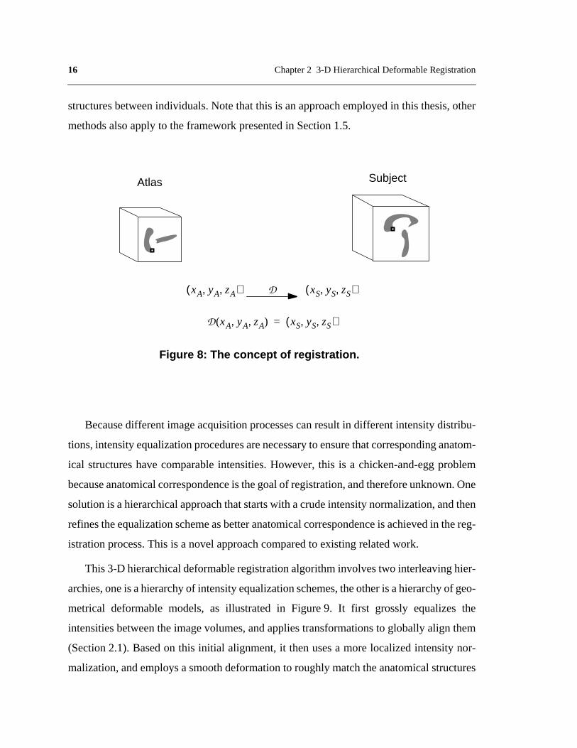
CHAPTER2 3-D HierarchicalDeformableRegistration
This chapterintroducesa 3-D deformableregistrationmethodthat doesnot utilize
knowledgeof anatomicalvariations.This algorithm will bootstrapthe closed-loopof
extractingknowledgefor guidingregistration,andfunctionasa baselinefor performance
comparisons.
The3-D registrationalgorithmmatchesimagevolumesbasedon intensitycorrespon-
dence.Thetaskof registrationis to find a3-D deformationfunction thatmapsanypar-
ticular atlasvoxel to the correspondingvoxel in the subject’s
volume,illustratedin Figure8.Asmentionedin section1.4,therearenotonly intrinsicana-
tomical differencesbetweenpeople’sMRIs, but alsoextrinsicdifferencesresultedfrom
different imageacquisitionprocesses.Therefore,a hierarchicalschemeis adoptedto first
addressthe extrinsic variations,and then deformablymatch correspondinganatomical
D
xA yA zA, ,( ) xS yS zS, ,( )
16 Chapter 2 3-D Hierarchical Deformable Registration
structures between individuals. Note that this is an approach employed in this thesis, other
methods also apply to the framework presented in Section 1.5.
Because different image acquisition processes can result in different intensity distribu-
tions, intensity equalization procedures are necessary to ensure that corresponding anatom-
ical structures have comparable intensities. However, this is a chicken-and-egg problem
because anatomical correspondence is the goal of registration, and therefore unknown. One
solution is a hierarchical approach that starts with a crude intensity normalization, and then
refines the equalization scheme as better anatomical correspondence is achieved in the reg-
istration process. This is a novel approach compared to existing related work.
This 3-D hierarchical deformable registration algorithm involves two interleaving hier-
archies, one is a hierarchy of intensity equalization schemes, the other is a hierarchy of geo-
metrical deformable models, as illustrated in Figure 9. It first grossly equalizes the
intensities between the image volumes, and applies transformations to globally align them
(Section 2.1). Based on this initial alignment, it then uses a more localized intensity nor-
malization, and employs a smooth deformation to roughly match the anatomical structures
SubjectAtlas
Figure 8: The concept of registration.
xA yA zA, ,( ) D xS yS zS, ,( )
D xA yA zA, ,( ) xS yS zS, ,( )=

17
in theimagevolumes(Section2.2).Thiscorrespondenceallowsamoreinformedintensity
transformationbetweenthetwo imagevolumes,anda fine-tuningdeformationadjuststhe
correspondenceof anatomicalstructuresmoreprecisely(Section2.3). This algorithm is
automatedby a randominitialization method(section6.3). Iterative optimizationalgo-
rithms are used to determine the deformation parameters at all levels.
2.1 Global alignmentwith whole volume intensity equalization
Thefirst level deformablemodeladjuststheextrinsicvariationsbetweentheatlasand
thesubject’simagevolume.Becausetheextrinsicvariationscorresponddifferencesin ori-
entation,position,andscaleof the imagevolumes,a similarity transformationcomposed
of 3-D rotation, translation, and uniform scaling is sufficient to compensate for them.
As mentionedearlier,differentimagingprocessesmayresultin differentintensitydis-
tributionsin the atlasandthe subjectvolume.This differencecanmakea methodusing
intensitycorrespondenceunreliable,asshownin the examplein Figure4. Beforeglobal
alignment,the imagevolumescanbe of significantly different orientation,position,and
scale.With unknowngeometricalcorrespondence,thefirst level intensityequalizationis a
wholevolumeintensitynormalization.It equalizesthemeanandstandarddeviationof the
intensitiesin theheadvolumesto roughlycorrecttheintensitydiscrepancy.Theheadvol-
umes are separated from the background in preprocessing (Section6.1).
2.1.1 Representing similarity transformation
Figure10 showsthecoordinatesystemsusedin thesimilarity transformation,T. The
originsof thecoordinatesystemsin theatlasandthesubjectvolumeareplacedattheircen-
troids(centerof massof theheadvolumes).TheZ axiscoincidewith theaxisalongwhich
thecross-sectionswerescanned.NotethattheZ axisdo not necessarilycoincidewith any
principalaxes,asdiscussedin section1.4.1.Theatlasis first rotatedaboutits origin to the
sameorientationof thesubjectvolume,thenuniformly scaledaboutits origin to beof the

18 Chapter 2 3-D Hierarchical Deformable Registration
Global Alignment
SmoothDeformation
Fine-tuningDeformation
Figure 9: 3-D Hierarchical Deformable Registration withtwo interleaving hierarchies: a deformation hierarchy andan intensity equalization hierarchy.
Structure-based Intensity Transformation
Whole Volume Intensity Equalization
Local Intensity Equalization
Atlas Subject

19
sameoverallsize,andthentranslatedto alignwith thesubjectvolume.Thesimilarity trans-
formationT has 7 degrees of freedom.
2.1.2 Determining similarity transformation
Becausetheatlasandthesubjectareinherentlydifferent,thereis nosimilarity transfor-
mationthatexactlymatchesthem.Thebesttransformationonly minimizesthedifferences.
The quality of a transformationis measuredby the sum of squareddifferences(SSD)
betweentheintensitiesof geometricallycorrespondingvoxelsin theimagevolumes[111].
Suppose is theintensityof voxel in thesubject’svolume.Thesim-
ilarity transformationT matches to in theatlas,and is
the intensity at in the atlas.The squareddifferencebetween and
is summed over the whole volume to compute SSD:
Z
Y
X
Z
CentroidCentroid
Figure 10: Coordinate systems used in the similarity transformation.
Y
X
Atlas Subject
I s x y z, ,( ) x y z, ,[ ]s
x y z, ,[ ]s T x y z, ,( )a Ia T x y z, ,( )( )
T x y z, ,( )a I s x y z, ,( )
Ia T x y z, ,( )( )
SSD I s x y z, ,( ) I a T x y z, ,( )( )–( )2
x y z, ,( )∑= (1)
20 Chapter 2 3-D Hierarchical Deformable Registration
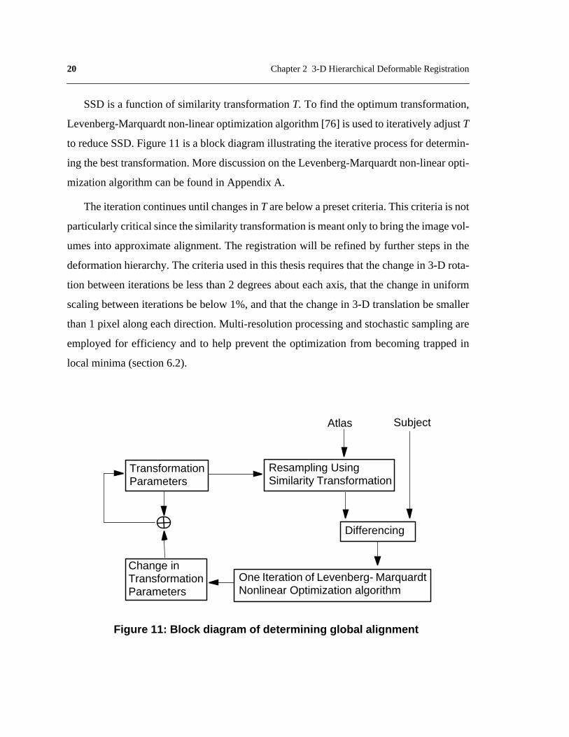
SSD is a function of similarity transformation T. To find the optimum transformation,
Levenberg-Marquardt non-linear optimization algorithm [76] is used to iteratively adjust T
to reduce SSD. Figure 11 is a block diagram illustrating the iterative process for determin-
ing the best transformation. More discussion on the Levenberg-Marquardt non-linear opti-
mization algorithm can be found in Appendix A.
The iteration continues until changes in T are below a preset criteria. This criteria is not
particularly critical since the similarity transformation is meant only to bring the image vol-
umes into approximate alignment. The registration will be refined by further steps in the
deformation hierarchy. The criteria used in this thesis requires that the change in 3-D rota-
tion between iterations be less than 2 degrees about each axis, that the change in uniform
scaling between iterations be below 1%, and that the change in 3-D translation be smaller
than 1 pixel along each direction. Multi-resolution processing and stochastic sampling are
employed for efficiency and to help prevent the optimization from becoming trapped in
local minima (section 6.2).
Atlas Subject
Figure 11: Block diagram of determining global alignment
Resampling UsingSimilarity Transformation
Differencing
One Iteration of Levenberg- MarquardtNonlinear Optimization algorithm
TransformationParameters
Change inTransformationParameters

21
Note that the transformedatlas coordinates, , may not be integral, and
will not begivenby theoriginal data.In this case,tri-linear interpolationis
usedto determinethevoxel’s intensityfrom its eightboundingneighbors,seeFigure12.If
falls outside of the volume, that voxel is ignored for the SSD computation.
Figure13 showsanexampleof globally aligningtheatlasto a particularsubject.The
first row areexampleslicesof theatlasandthesubject’svolumebeforetheglobalalign-
ment.Theatlasis thenresampledto matchthesubject’svolumevia a similarity transfor-
mation,andcorrespondingslicesareshownon thesecondrow. Notethat theatlasis now
of thesameorientation,scale,andpositionasthesubject’svolume.Thesegmentationof
onebrainstructure,thecorpuscallosum,is adaptedfor thesubjectunderthesametransfor-
mation.The outline of the corpuscallosumis shownin the resampledatlas,anddirectly
appliedto thesubject’svolume.Note thatalthoughthe two volumesaregrosslyaligned,
theexamplestructuredoesnot matchwell with its counterpart.This is becausethereexist
Linear interpolationsamong 8 neighborsalong one axis gives 4intermediate values
Linear interpolationamong the 4 interme-diate values along an-other axis then yields 2intermediate values
Linear interpolationbetween the 2 inter-mediate values alongthe third axis gives thevoxel intensity
Figure 12: Trilinear Interpolation gives the intensity of a voxel withnon-integral coordinates by doing linear interpolations among its 8bounding neighbors along each of the three axes.
T x y z, ,( )a
Ia T x y z, ,( )( )
T x y z, ,( )a

22 Chapter 2 3-D Hierarchical Deformable Registration
intrinsic anatomicaldifferencesbetweenindividuals,as discussedin Section1.4.2,and
globalalignmentonly addressesextrinsicdifferencescausedby separateimageacquisition
processes.
2.2 Smooth deformationwith local intensity equalization
Theglobalalignmentadjustsextrinsicvariationsbetweenimagevolumes,but cannot
addressintrinsicvariationsbetweenindividualstructures,asshownin Figure13.Transfor-
mationsthatallow localdeformationsarenecessary.An intuitive solutionis to allow each
voxel to shift freely in 3-D spaceto alignwith its counterpart.But thiswill requirethevox-
els’ initial positionsto be closeto their desiredpositionsso asnot to be trappedin local
minima.Sincetheglobalalignmentcannotguaranteea preciseenoughinitial correspon-
dencefor individual structures,thesecondlevel deformablemodeltakesan intermediate
step which allows 3-D deformation at a local neighborhood level.
Theintensityequalizationschemecanberefinednowthatthereis moreinformationon
the correspondencebetweenthe two volumes.The secondlevel intensity equalization
evensthe intensitymeanandstandarddeviationbetweentheoverlappingportionsof the
atlasandthesubjectvolumeafter theyareglobally aligned.Similar to thecasein global
alignment,intensitydifferencesbetweencorrespondingvoxelsin thesubjectvolumeand
theatlasactasthedeformingforce,whichshift voxelneighborhoodsin 3-D spaceto align
with their counterparts.
2.2.1 Representing smooth deformations
To representlocal deformationsat a neighborhoodlevel, thesmoothdeformationpro-
cedureusesa3-Dcontrolgridwhichisacoarsergrid thanthevoxelgrid.Controlgridsused
in thisthesisaregeneratedby regularlysub-samplingthevoxelgrid,soeachcell in thecon-
trol grid is aparallelepipedor acube.Verticesof thecontrolgrid arecontrolpointsthatcan
shift independentlyin 3-D space.3-D displacementsof thecontrolpointsaredeformation

23
Figure 13: Global alignment matc hes the atlas to the subject’ svolume , and adapts segmentations of brain structures for thesubject. Ho wever, individual structures do not align well.
CorpusCallosum
Atlas Subject
Global Alignment

24 Chapter 2 3-D Hierarchical Deformable Registration
parameterswhichdeterminethedisplacementsof thevoxelstheyenclose.This imposesan
implicit smoothnessonthedisplacementfield. Sincethenumberof controlpointsis orders
of magnitudelower thanthenumberof voxels,this representationmakesthedeformation
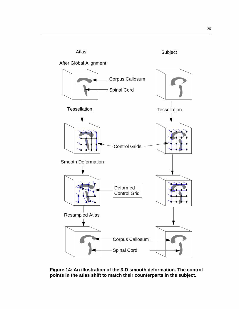
optimizationprocessmorestable.Figure14illustratesthe3-Dsmoothdeformation.Adapt-
ablemulti-resolutionprocessingandstochasticsamplingareagainemployedfor efficiency
andto helppreventtheoptimizationfrom becomingtrappedin localminima(section6.2).
Thehighestresolutioncontrolgrid employedis 7x7x7.Szeliskiusedsimilarapproachesin
2-D imageregistrationand3-D surfaceregistration[89], [90]. Vemuri et al. proposedan
analoguesschemefor motionanalysis[102]. Collinsetal. employed3-D gridsfor feature-
basedregistration,thoughdeformationof the grid is constrainedto a local affine model
[14].
2.2.2 Estimating smooth deformation
Similar to the casefor global alignment,the goodnessof the smoothdeformationis
measuredby theSSDbetweenintensitiesof correspondingvoxelsin theatlasandthesub-
ject volume.For a voxel at in thesubjectvolume,supposeit belongsto the ith
controlcell . Thecontrolcell of thesameindexin theatlasis . Fromthe
relativepositionof voxel with respectto theeightverticesof in thesub-
ject’svolume,thelocationof its correspondingvoxel in theatlas, , canbedeter-
mined:assumethesamerelativepositionholdsbetweenvoxel andcontrolcell
in theatlas,tri-linearly interpolatetheposition from theeightvertices
of . HereS denotessmoothdeformation.In thecasethat doesnot fall
onthevoxelgrid, theintensityof voxel is tri-linearly interpolatedfrom its eight
neighboringvoxelsin theatlas.NotethattheintensitySSDis computedoverall voxelsin
the atlas and the subject volume, not just for the control points.
If theatlascompletelyalignswith thesubjectvolume,intensitiesbetweencorrespond-
ing voxelsshouldbe equal.However,in practicethey may differ. The bestdeformation
minimizesthe intensity SSD.Similar to section2.1.2,a Levenberg-Marquardtiterative
non-linearoptimizationmethodis usedto determinethebestsmoothdeformationparame-
x y z, ,[ ]s
Cells i[ ] Cella i[ ]
x y z, ,[ ]s Cells i[ ]
S x y z, ,( )a
S x y z, ,( )a
Cella i[ ] S x y z, ,( )a
Cella i[ ] S x y z, ,( )a
S x y z, ,( )a
25
Corpus Callosum
Spinal Cord
After Global Alignment
Figure 14: An illustration of the 3-D smooth deformation. The controlpoints in the atlas shift to match their counterparts in the subject.
Atlas
Resampled Atlas
Subject
Corpus Callosum
Spinal Cord
Smooth Deformation
DeformedControl Grid
Tessellation Tessellation
Control Grids

26 Chapter 2 3-D Hierarchical Deformable Registration
ters.Figure15 is a block diagramillustratingtheiterativeoptimizationprocessof smooth
deformation.
Thebestsmoothdeformationis consideredto bedeterminedwhenthechangeof each
parameterdropsbelow a presetthreshold.The thresholdusedin this thesisis that the
changeof eachcontrolpoint’spositionalongeachof the3-D directionsbetweeniterations
is below 1 voxel unit. Control grids and imagevolumesin multi-resolutionareusedto
improve efficiency and avoid local minima, which will be discussed in 6.2.
Figure16 showstheeffectof applyingsmoothdeformationto the intermediateresult
afterglobalalignment.Theatlasis warpedin 3-D to matchwith thesubjectvolume.Seg-
mentationof corpuscallosumis furtheradaptedfor thesubject.Whendirectly appliedto
the subjectvolume,its outline roughly alignswith the subject’scorpuscallosum.Com-
paredto the resultafter global alignment,the registrationfor individual brain structures
Atlas Subject
Figure 15: Block diagram of smooth deformation
Resampling UsingSmooth Deformation
ControlPoints
Differencing
One Iteration of Levenberg- MarquardtNonlinear Optimization algorithm
Change in Control Points’3-D Displacements

27
improved significantly, but there still exists misalignment at fine details. This is because
smooth deformation implicitly enforces local neighborhoods to deform coherently.
Figure 16: Smooth deformation impr oved the alignment of individualstructures between the atlas and the subject’ s volume
CorpusCallosum
Atlas Subject
After Global Alignment
Smooth Deformation

28 Chapter 2 3-D Hierarchical Deformable Registration
2.3 Fine-tuning deformationwith linear intensity transformation
Smoothdeformationonly allowscontrolpointsto shift freely in 3-D space,displace-
mentsof voxels insidecontrol grid cells aredeterminedby the boundingcontrol points.
Thismeansgeometricaldifferencesbetweentheatlasandthesubjectthataresmallerthan
thesizeof a controlgrid cell cannotbeadjusted.This necessitatesthe last level of defor-
mation.It fine-tunesthe3-D alignmentby permittingeachvoxel to shift independentlyin
3-D spaceto matchwith its counterpart.Notethatthis is aspecialcaseof thesmoothdefor-
mation in which the control grid is the voxel grid, and each voxel is a control point.
Theimprovedalignmentof individual anatomicalstructuresaftersmoothdeformation
enablesa morepreciseintensityequalizationbetweenthe atlasand the subjectvolume.
Fromobservation,thematchis generallymorereliablefor structureswith relatively sim-
pler shapeanddistinct intensity, suchascorpuscallosumandskull. Corpuscallosumdis-
playsahighsignalintensity, whereasskull hasalow signalintensity, asshown in Figure17.
Their representativeintensitiescanjointly determinea lineartransformationthatequalizes
the two volumes’intensitydistributions.Figure18 displaysintensityhistogramsof these
two structuresin theatlas,andhistogramsof whatwasautomaticallysegmentedascorpus
callosumandskull in thesubject’svolume.Therepresentativeintensityof corpuscallosum
is definedasthehighestpeakin its intensityhistogramafterGaussiansmoothing,andthe
representative intensityof skull is denotedasthelowestpeakin its smoothedintensityhis-
togram.Theserepresentative intensitiesfrom theatlasandthesubjectform a linearinten-
sity transformationbetweenthem.This transformationfurtherequalizesthe intensitiesin
the atlas and the subject’s volume.
2.3.1 Representing fine-tuning deformation
Similar to globalalignmentandsmoothdeformation,theintensitydifferencebetween
spatiallycorrespondingvoxelsin theatlasandthesubject’svolumeservesasthedeforming
force.What is different is thatnow eachvoxel canshift independentlyin 3-D space.The

29
deformationparametersare3-D displacementsof all voxels,which is 3 timestheamount
of intensity data. Note that this is an under-constrained problem.
2.3.2 Estimating fine-tuning deformation
SupposeD denotesthe currentfine-tuningdeformation. For a voxel in the
subject’svolumewith intensity , its correspondingvoxel in theatlas
hasintensity . Considerthe casethat correspondingvoxels havethe same
intensity,andtheoptimumdeformationis achievedonestepfrom D. Use to denotethe
difference betweenD and the optima, we have:
The first order Taylor expansion of the left-hand-side in (2) gives:
Figure 17: Corpus Callosum has a high signal intensity (bright),and skull has a low signal intensity (dark).
Skull
CorpusCallosum
x y z, ,[ ]s
I s x y z, ,( ) D x y z, ,( )a
Ia D x y z, ,( )( )
Dδ
I a D x y z, ,( ) δD x y z, ,( )+( ) I s x y z, ,( )= (2)
I a D x y z, ,( )( ) I a∇ D x y z, ,( )( )[ ]T δD+ (3)

30 Chapter 2 3-D Hierarchical Deformable Registration
is thefirst orderderivative,i.e. imagegradient,at voxel in
the atlas. Substitute (3) into (2) gives theimage brightness constraint [77]:
Figure 18: Intensity histograms of corpus callosum (top) inthe atlas (dotted line) and the subject’ s volume (solid line),as well as the corresponding ones of skull (bottom).
0 50 100 150 200 250 3000
0.01
0.02
0.03
0.04Corpus Collasum Intensity Histogram
Intensity
Fra
ctio
n o
f V
oxe
ls
atlas patient
0 50 100 150 200 250 3000
0.005
0.01
0.015
0.02Skull Intensity Histogram
Intensity
Fra
ctio
n o
f V
oxe
ls
atlas patient
Ia D x y z, ,( )( )∇ D x y z, ,( )a
I a D x y z, ,( )( ) I a∇ D x y z, ,( )( )[ ]T δD I s x y z, ,( )–+ 0=

31
The above equation yields one solution for:
To stabilize the deformationparameterswhen the intensity gradient in the atlas,
, is close to zero, a stabilizing factor is added:
ThedeformationD is recoveredby computing , addingit to D, anditeratinguntil
is smallerthana presetthreshold.In the currentimplementation,the iterationstops
when the root-mean-square(RMS) betweenthe intensitiesof spatially corresponding
voxelsbetweentwo iterationsdecreasesby lessthan0.5%.3-D isotropicGaussiansmooth-
ing is appliedto thevolume’s3-D displacementflow aftereachiterationto regularizethe
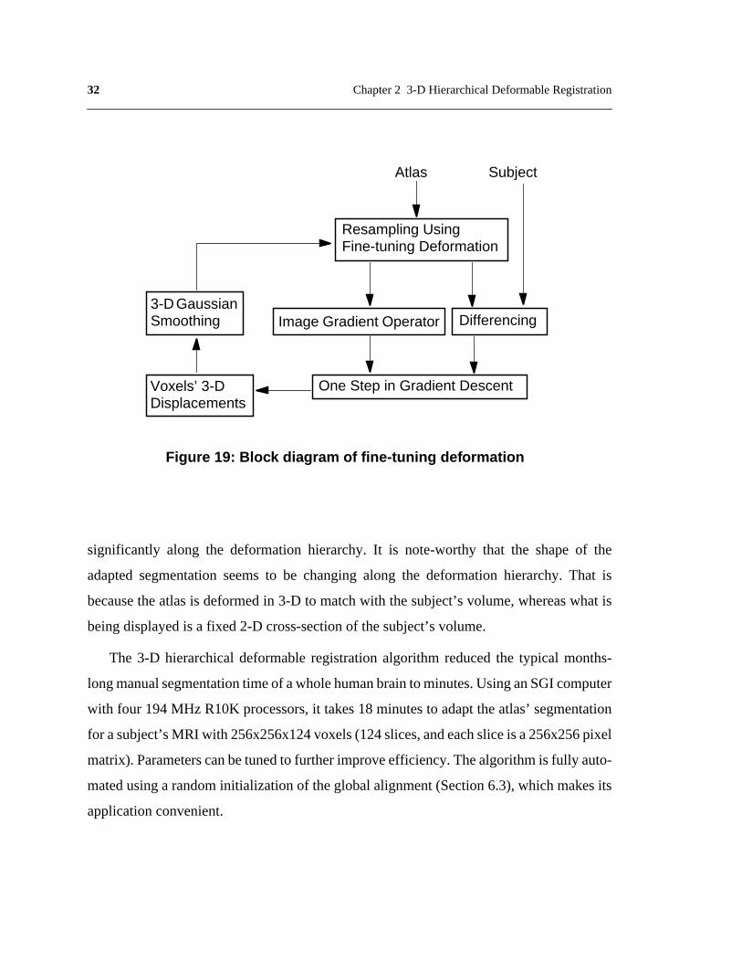
under-constrainedproblem.Thirion usedasimilarapproach[92]. Figure19showsablock
diagram that illustrates the fine-tuning deformation procedure.
Figure20 showsthe effect of applying fine-tuning deformationto the intermediate
resultaftersmoothdeformation.Theatlasis furtherwarpedto matchwith thesubject’svol-
ume.Thesegmentationof corpuscallosumis adaptedto matchbetterwith thestructurein
the subject’s data.
Anotherexampleof registeringthe atlaswith a subject’sdatausing the hierarchical
deformableregistrationis displayedin Figure21.Segmentationof anatomicalstructuresis
alsoadaptedfor thesubject,andoutlinesof severalstructures,e.g.thepair of lateralven-
tricles,areprojectedontothesubject’sdatato illustratetheimprovementin matchingindi-
vidualstructures.Figure22is aclose-upof thesubject’slateralventriclesin Figure21.The
alignmentbetweentheadaptedsegmentationandthesubject’slateralventriclesimproves
Dδ
δDI s x y z, ,( ) I a D x y z, ,( )( )–
I a D x y z, ,( )( )∇ 2--------------------------------------------------------------------------- I a D x y z, ,( )( )∇= (4)
Ia D x y z, ,( )( )∇ α
δDI s x y z, ,( ) I a D x y z, ,( )( )–
I a D x y z, ,( )( )∇ 2 α+--------------------------------------------------------------------------- I a D x y z, ,( )( )∇=
(5)
Dδ
Dδ
32 Chapter 2 3-D Hierarchical Deformable Registration
significantly along the deformationhierarchy.It is note-worthy that the shapeof the
adaptedsegmentationseemsto be changingalong the deformationhierarchy.That is
becausetheatlasis deformedin 3-D to matchwith thesubject’svolume,whereaswhat is
being displayed is a fixed 2-D cross-section of the subject’s volume.
The 3-D hierarchicaldeformableregistrationalgorithm reducedthe typical months-
longmanualsegmentationtimeof awholehumanbrainto minutes.UsinganSGIcomputer
with four 194MHz R10K processors,it takes18 minutesto adapttheatlas’segmentation
for asubject’sMRI with 256x256x124voxels(124slices,andeachsliceis a256x256pixel
matrix).Parameterscanbetunedto furtherimproveefficiency.Thealgorithmis fully auto-
matedusinga randominitializationof theglobalalignment(Section6.3),whichmakesits
application convenient.
Atlas Subject
Figure 19: Bloc k dia gram of fine-tuning def ormation
Resampling UsingFine-tuning Deformation
Differencing
One Step in Gradient DescentVoxels’ 3-DDisplacements
Image Gradient Operator3-D GaussianSmoothing

33
Figure 20: Fine-tuning deformation further improvesregistration accuracy of anatomical structures.
CorpusCallosum
After Smooth Deformation
Fine-tuning Deformation
Atlas Subject

34 Chapter 2 3-D Hierarchical Deformable Registration
After Global Alignment
After Fine-Tuning Deformation
After Smooth Deformation
LateralVentricles
LateralVentricles
LateralVentricles
Figure 21: The progressive results of hierarchical deformation.
Atlas Subject

35
2.4 Quantitative evaluation
Qualitatively,registrationresultsshownin Figure20 andFigure22 areencouraging,
however,objectiveandquantitativeevaluationis necessary.Forrigid registration,transfor-
mationparameterscanbecomparedto thosederivedfrom stereotaxicfiducial markersrig-
idly fixed to asubject’sskull [110].Althoughfiducial-basedregistrationitself hasinherent
measurementerrors,it is generallyadoptedas a ground-truth transformation.Unfortu-
nately,no suchground-truth canbe acquiredfor deformableregistration.Onecommon
solutionis to assesshow well theadaptedsegmentationfrom anatlasmatchesthecorre-
spondinganatomicalstructurein thesubject’simagevolume.In this way, thedemandfor
Deformation Hierarchy
Figure 22: A close-up on the subject’ s lateral ventric les in Figure 21.The alignment between the adapted segmentation fr om the atlasand the subject’ s structures impr ove significantl y.
Global Alignment
Smooth Deformation
Fine-tuning Deformation
36 Chapter 2 3-D Hierarchical Deformable Registration
ground-truth deformation becomestherequirementfor ground-truth segmentation of the
subject’s anatomical structures.
2.4.1 Ground-truth segmentation
In vivo data,thekind of datausedin this thesis,presentsanotherdifficulty to quantita-
tive validation:ground-truth segmentation of anatomicalstructuresin living peopleis not
available.As a solution,expertsegmentationandclassificationof a subject’sanatomical
structuresare regardedas ground-truth, or the gold-standard. A similar approachwas
employed in [2], [14], [19], and [33].
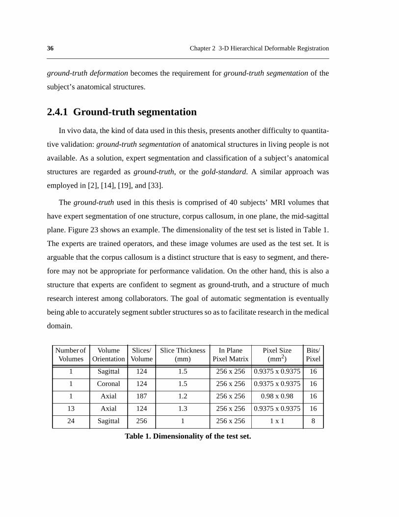
The ground-truth usedin this thesisis comprisedof 40 subjects’MRI volumesthat
haveexpertsegmentationof onestructure,corpuscallosum,in oneplane,themid-sagittal
plane.Figure23 showsanexample.Thedimensionalityof thetestsetis listedin Table1.
The expertsaretrainedoperators,andtheseimagevolumesareusedasthe testset.It is
arguablethatthecorpuscallosumis a distinctstructurethat is easyto segment,andthere-
fore maynot beappropriatefor performancevalidation.On theotherhand,this is alsoa
structurethat expertsareconfidentto segmentasground-truth,anda structureof much
researchinterestamongcollaborators.The goal of automaticsegmentationis eventually
beingableto accuratelysegmentsubtlerstructuressoasto facilitateresearchin themedical
domain.
NumberofVolumes
VolumeOrientation
Slices/Volume
Slice Thickness(mm)
In PlanePixel Matrix
Pixel Size(mm2)
Bits/Pixel
1 Sagittal 124 1.5 256 x 256 0.9375x 0.9375 16
1 Coronal 124 1.5 256 x 256 0.9375x 0.9375 16
1 Axial 187 1.2 256 x 256 0.98 x 0.98 16
13 Axial 124 1.3 256 x 256 0.9375x 0.9375 16
24 Sagittal 256 1 256 x 256 1 x 1 8
Table 1. Dimensionality of the test set.

37
Someresearchersvalidatetheirmethodsby registeringoneimagevolumewith atrans-
formedversionof itself, andcomparingthecomputedtransformationto theknowntrans-
formation.Note that when the known transformationis of the sameformulation as the
transformationusedin theregistrationprocess,this schemeis testingthealgorithm’scon-
sistency, but not the accuracy.
2.4.2 Measurement
Currently,thereis nostandardmetricfor evaluatingsegmentationaccuracy.Dannetal.
introduceda relativeoverlapmeasurefor comparingtwo segmentationswhenneitheris
necessarilycorrect.It is definedastheratiobetweentheareaof intersectionandtheareaof
theirunion[19]. Collinsetal. usedthreemeasuresto evaluatesegmentationaccuracy[14].
Oneis theratioof absolutevolumedifferencebetweenground-truthandthecomputedseg-
mentationw.r.t. ground-truth.Sincea smallvolumedifferencedoesnot indicateaccurate
segmentation,anothermeasureis definedastheratiobetweentheoverlappingvolumeand
ground-truth.However,thismeasuregives100%for anaccuratesegmentationor anyseg-
mentationthat is a supersetof ground-truth.This necessitatesthethird measure,which is
Figure 23: An example of expert segmentationof corpus callosum in the mid-sagittal plane.

38 Chapter 2 3-D Hierarchical Deformable Registration
theratio betweentheoverlappingvolumeandthecomputedsegmentation.Thesmallerof
thesecondandthird measureis usedfor validation.Bajcsyet al. employedthenumberof
correctlymatchedvoxels,falsepositives,andfalsenegativesto assesstheperformanceof
their globalmatchingprocedure[2]. Geeet al. examinedsegmentationof 32 corticaland
subcorticalstructuresin a testsetof 6 subjects,usingtherelativeoverlapmeasurein [19]
andthesecondmeasurein [14]. In addition,theyemployedthedistancebetweenthecen-
troidsof asegmentationandits ground-truthto indicatethelocalizationaccuracy[33]. For
feature-basedregistration,Davatzikosdefinedtheregistrationerrorateachfeaturepointor
landmark to be the distance between its computed location and its ground-truth [20].
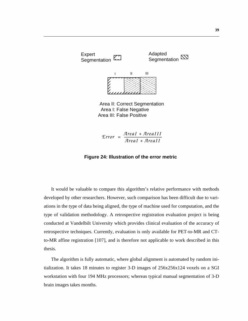
In this thesis,segmentationerroris measuredby theratio betweenthenumberof mis-
labelledvoxelsandground-truth,as illustratedin Figure24. The numberof mislabelled
voxelsincludesbothfalsepositives,i.e. voxelsclassifiedascorpuscallosumby thealgo-
rithm butnot in theground-truth,andfalsenegatives,i.e.voxelsclassifiedascorpuscallo-
sumin the ground-truthbut not by the algorithm.Note that this error canbe biggerthan
100%.If thethreeareasin Figure24areof equalsize,thenthiserrorwill be100%,whereas
[19]’s relativeoverlapmeasurewill be33%,andmeasuresdefinedin [14] will give zero
volumedifferenceand50%overlap.Theerrormeasureddefinedhereis thereforethemost
stringent.
2.4.3 Performance
Theperformanceevaluationprocessinvolvesapplyingthe3-D hierarchicaldeformable
registrationalgorithmto matchthe atlasto eachimagevolume in the test set,and thus
adaptingtheatlas’anatomicalsegmentationrespectively.Overallerror ratio of thewhole
testsetis computedateachlevelof thedeformationhierarchy,andcomparedin Figure25.
For the final resultafter fine-tuningdeformation,the algorithmreachedan overall error
ratioof 4.4%.This is asignificantreductionoverthe22.8%erroryieldedby smoothdefor-
mation,andadrasticreductionoverthe55.5%errorafterglobalalignment.Thisquantita-
tive assessment of registration accuracy validates the observation in Figure22.
39
It would be valuableto comparethis algorithm’srelativeperformancewith methods
developedby otherresearchers.However,suchcomparisonhasbeendifficult dueto vari-
ationsin thetypeof databeingaligned,thetypeof machineusedfor computation,andthe
type of validation methodology.A retrospectiveregistrationevaluationproject is being
conductedat VandelbiltUniversitywhich providesclinical evaluationof theaccuracyof
retrospectivetechniques.Currently,evaluationis only availablefor PET-to-MRandCT-
to-MR affine registration[107], andis thereforenot applicableto work describedin this
thesis.
Thealgorithmis fully automatic,whereglobalalignmentis automatedby randomini-
tialization. It takes18 minutesto register3-D imagesof 256x256x124voxelson a SGI
workstationwith four 194MHz processors;whereastypical manualsegmentationof 3-D
brain images takes months.
�����������������������������������������������������������������������������������������������
I II III
AdaptedSegmentation
Error AreaI AreaIII+AreaI AreaII+
------------------------------------------------=
ExpertSegmentation
�
Area II: Correct SegmentationArea I: False Negative
Area III: False Positive
Figure 24: Illustration of the error metric

40 Chapter 2 3-D Hierarchical Deformable Registration
2.5 Error analysis
Errorsin segmentationcanbecausedby severalsources.Oneis biasincurredby using
manuallysegmentedstructuresfrom a singleindividual asthemodelatlas.Any errorsin
theatlasarecarriedthroughthedeformableregistration,yieldingerrorsin thesegmentation
of subjects’data.This will betruein generalfor anyatlasdefinedon thebasisof a single
brain,andcanonlybecompensatedwhentheatlasisextendedto representanatomicalvari-
ationsbetweenindividuals.Anothersourceis inter-subjectinter-observervariability. Ana-
Global Alignment Smooth Deformation Fine−tuning Deformation0
10
20
30
40
50
60
% o
f mis
labe
lled
voxe
ls
Figure 25: Overall error ratio of the test setat each level of the deformation hierarchy.

41
tomical differencesbetweenindividuals complicatethe manualsegmentationprocesses
involvedin creatingtheground truth andtheatlas.Definition of thecorpuscallosumvaries
from expertto expert,from subjectto subject.Segmentationsfrom multipleexpertscanbe
integratedto improveconsistency.Finally, errorsfrom deformableregistration.Sincegeo-
metriccorrespondenceis establishedbasedon intensitycorrespondence,anydiscrepancy
in intensitycanleadto errorsin registration.Improvementof theregistrationalgorithmwill
be further discussed in the following chapters.
2.6 Algorithm analysis
While it is validatedthatregistrationaccuracyimprovesalongthedeformationhierar-
chy, it is alsoimportantto assessthe effectivenessof the intensityequalizationscheme.
Moreover,while the overall error ratio revealsthe algorithm’sperformance,it is still of
interest to examine the distribution of error over the test set.
2.6.1 Effectiveness of intensity equalization
Threeexperimentsaredesignedto assesstheefficacyof theintensityequalizationhier-
archy,asshownin Table2.Theseexperimentsareconductedoverthewholetestset.Over-
all errorratiosshowthatthefirst andsecondlevelsof intensityequalizationgenerallyhelp
theregistrationto reduceerrorby 6%.Thethird level,structure-basedequalization,proves
to beremarkablyeffective.It broughttheerror ratefrom 26.2%to 4.4%,which is a 83%
errorreduction.Thisdemonstratesthatsmoothdeformationis ableto aligntheatlasandthe
subject’svolumewell enoughfor thestructure-basedequalizationto bereliable.Notethat
registrationresultsdeterioratedby15%whenfine-tuningdeformationwasperformedwith-
out thestructure-basedintensityequalization.Thisvalidatesthenecessityfor thestructure-
basedequalization,andprovestheeffectivenessof interleavinganintensitynormalization
hierarchy with a 3-D deformation hierarchy.

42 Chapter 2 3-D Hierarchical Deformable Registration
2.6.2 Error distribution
Histogram distribution of error ratios over the test set is computed at each level of the
deformation hierarchy, and displayed in Figure 26. After global alignment only 14.6% of
all samples have an error ratio below 20%. After smooth deformation 43.9% of all samples
have less than 20% error, and 14.6% of all samples have an error ratio below 10%. Fine-
tuning deformation eliminated cases with more than 20% error, and brought 92.7% of all
samples to an error ratio below 5%. The increase in registration accuracy is evident.
2.7 Discussion
So far the discussion has been focused on the design and evaluation of the hierarchical
deformable registration algorithm, and its interleaving intensity equalization scheme. It is
also interesting to remark on certain considerations and alternative approaches investigated
during the design.
Experiment Geometric Transformation Intensity Equalization Error Ratio
1 Global AlignmentNone 61.3%
Whole-volume equalization 55.5%
2Global Alignment
Smooth Deformation
Whole-volume equalization 25.6%
Whole-volume equalization& Local equalization
22.8%
3Global Alignment
Smooth DeformationFine-tuning Deformation
Whole-volume equalization& Local equalization
26.2%
Whole-volume equalization& Local equalization
& Structure-based equalization4.4%
Table 2. Evaluating the effectiveness of the intensity equalization hierarchy

43
2.7.1 Transformation and resampling
To registerthe atlaswith a particularsubject’svolume, the transformationscan be
eitherfrom theatlas’coordinateframeto thesubject’s,or vice versa.However,for appli-
cationsthatneedthesegmentationandclassificationof thesubject’sanatomicalstructures,
it is necessaryto resamplethe atlasinto the subject’scoordinateframeso asto adaptits
expertsegmentationandclassificationfor thesubject.This resamplingwill bestraightfor-
10 20 30 40 50 60 70 80 90 100 110 120 130 140 1500
10
20
30
40
50
60
70
80
90
100
Per
cen
tag
e o
f T
est
Cas
es
Ratio of Mislabelled Voxels to Correct Size
Global Align Smooth Fine−Tuning
Figure 26: Histogram distribution of error ratio overthe test set, at each level of the deformation hierarchy.
44 Chapter 2 3-D Hierarchical Deformable Registration
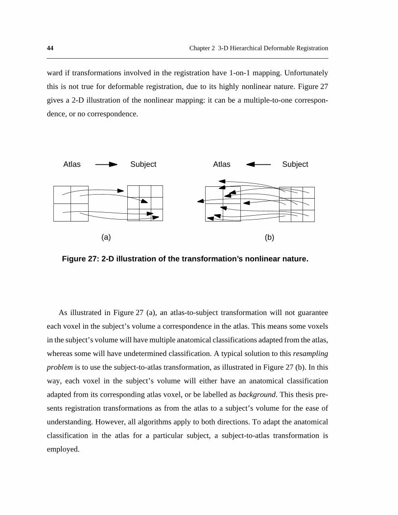
ward if transformationsinvolved in the registrationhave1-on-1mapping.Unfortunately
this is not true for deformableregistration,dueto its highly nonlinearnature.Figure27
givesa 2-D illustration of the nonlinearmapping:it canbe a multiple-to-onecorrespon-
dence, or no correspondence.
As illustratedin Figure27 (a), an atlas-to-subjecttransformationwill not guarantee
eachvoxel in thesubject’svolumea correspondencein theatlas.This meanssomevoxels
in thesubject’svolumewill havemultipleanatomicalclassificationsadaptedfromtheatlas,
whereassomewill haveundeterminedclassification.A typical solutionto this resampling
problem is to usethesubject-to-atlastransformation,asillustratedin Figure27 (b). In this
way, eachvoxel in the subject’svolume will either have an anatomicalclassification
adaptedfrom its correspondingatlasvoxel,or belabelledasbackground. This thesispre-
sentsregistrationtransformationsasfrom the atlasto a subject’svolumefor the easeof
understanding.However,all algorithmsapplyto bothdirections.To adapttheanatomical
classificationin the atlas for a particular subject,a subject-to-atlastransformationis
employed.
Figure 27: 2-D illustration of the transf ormation’ s nonlinear nature .
Atlas Subject
(a) (b)
Subject Atlas

45
2.7.2 Other intensity equalization methods
A number of intensity normalization schemes were explored before the final design,
such as using histogram equalization to remove bright and dark outliers, and using lateral
ventricles instead of skull in determining linear intensity transformation. Histogram equal-
ization did not prove superior to normalization of intensity mean and variance, whereas
intermediate segmentation of lateral ventricles were not reliable enough to facilitate com-
putation of the correct intensity transformation. A more rigorous intensity normalization
method should account for signal distortions that are unique to the MRI process. Wells et
al. developed an EM-segmentation algorithm that used an imaging model to account for
that, and Kapur et al. extended the theme by adding a regularizer to combat salt-and-pepper
noise [49], [106].
2.7.3 Smoothness of deformation
The assumption of smoothness in deformation guarantees that neighboring voxels in
the atlas be mapped to neighboring points in the target. Similar approaches were used by
Black and Anandan [6]. However, there exist neighboring points in unconnected structures
(such as on opposite sides of a sulcus, or on either side of the longitudinal fissure) that do
not need to be mapped to neighboring voxels in the subject. Therefore, it may be desirable
to allow a discontinuity in the transformation at internal brain structures, e.g. surfaces that
separate the cerebellum from the occipital lobe or that separate the temporal lobe from the
inferior frontal lobe.
2.7.4 Quantitative evaluation
Since the corpus callosum seems an easy structure to identify, quantitative evaluation
based on its segmentation may not be the most convincing. However, during this thesis
work, this has been the structure experts can segment confidently enough to provide as
ground truth. Although performance evaluation based on the segmentation of structures of
more complex shape will be more rigorous, it has been observed and reported that struc-

46 Chapter 2 3-D Hierarchical Deformable Registration
tures with a complex boundary shape are more difficult for people to segment than those
with a simple boundary [52]. People have a tendency to over- or under-estimate the bound-
ary. Consequently, manual segmentation exhibits a consistent variability in the segmenta-
tion of voxels at the boundary of complicated shapes such as the cortical grey matter.
2.8 Chapter summary
This chapter has presented and evaluated a 3-D hierarchical deformable registration
algorithm that does not use guidance of anatomical knowledge. This algorithm is a neces-
sary starting point to achieve the next goal, the characterization of brain anatomy and its
variations, which will be discussed in the next chapter.
47
CHAPTER3 Building a StatisticalAtlas
The 3-D hierarchical deformable registration algorithm discussedin Chapter 2
achieved encouragingperformance.However, considerableinaccuraciesstill exist.
Figure28 comparessegmentationresultsgivenby theautomaticalgorithmandthat from
anexpert.Notethatcertaininaccuraciesarecausedby thealgorithm’sinsufficientknowl-
edge of the anatomy, and cannot be corrected by exploiting image features solely.
Thisobservationis supportedby theanalysisin Section2.6,thatonemajorerrorsource
is biasintroducedby theatlas.Thecurrentatlas is not anaverageor representativemodel
of anypopulation,it is a singlenon-pathologicalbrainMRI whosestructuresweremanu-
ally classified.It is possiblethattheatlasis anextremeof thenormaldistribution.Thecur-
rent algorithm is matchingthis potentially biasedatlasto any particularsubject’sdata,
which is inevitablyerroneous.Moreover,asdiscussedin Section1.4.2,anatomicaldiffer-
encesbetweenindividualspresenta major difficulty to inter-subjectregistration.There-
fore, building an atlasbasedon multiple subjects’dataso that it representsthe average
brain aswell as its normalanatomicalvariability will help improve registrationperfor-
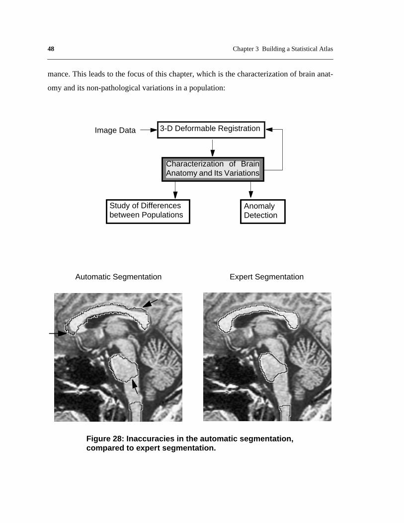
48 Chapter 3 Building a Statistical Atlas
mance. This leads to the focus of this chapter, which is the characterization of brain anat-
omy and its non-pathological variations in a population:
Study of Differencesbetween Populations
AnomalyDetection
Characterization of BrainAnatomy and Its Variations
3-D Deformable RegistrationImage Data
Automatic Segmentation Expert Segmentation
Figure 28: Inaccuracies in the automatic segmentation,compared to expert segmentation.

49
3.1 Related work
Techniquessolelybaseonimagefeatureshaveappearedinadequatefor manysegmen-
tation, registration,and measurementtasksin medical imaging. The inclusion of prior
knowledgein theanalysisprocedurehasbecomeincreasinglyimportant.Prior knowledge
mayconcernthephysicsof imageformation;theanatomy,pathologyor (patho)physiology
of theorgansor tissuesunderinvestigation;or theexpertiseof themedicalspecialistonthe
interpretation of the image data.
During thepastdecade,manyresearchershaveworkedonmodelingshapevariationof
organsor physiologicalvariationof tissuecharacteristics.Oneapproachis landmark-based
morphometricsfor multivariateanalysisof curvingoutlinesin biomedicalimages.In this
approach,shapesaredefinedasequivalenceclassesof discretepoint-setsundertheopera-
tion of theEuclideansimilarity group.A Procrustesdistancebetweeneverypairof shapes
is characterizedby a least-squaresformula.Booksteinintroduceda combinationof Pro-
crustesanalysisandthin-platesplinesto providea rangeof complementaryfilters, from
high passto low pass,for effectson outlineshapein groupedstudies[7]. He appliedthis
hybrid methodto comparetheshapeof thecorpuscallosumfrom mid-sagittalsectionsof
25 human brain MRIs, 12 normal and 13 with schizophrenia.
However,in any structuralanatomicaldataset therewill be moreinformationabout
structuraldifferencesthancanbecapturedby landmarks.Davatzikosetal. studiedcallosal
outlinesacquiredby anautomaticactivecontourmethod,andrelatetheoutlinesof samples
to ana priori normusingelasticrelaxation.Therelationof eachindividual to thenormis
thendescribedby an arealdistortionfunction,which capturesthe anatomicalvariability
[21]. Groups(eightmaleandeightfemale)arecomparedby averagingthedistortionatcor-
respondingpointsof thenormativeform or overregions,andthresholdingthedifferences
atvariouseffectsizes.SclaroffandPentlandrepresentedshapein termsof anobject’sphys-
ical deformationmodes.Therepresentationconsistsof two levels,oneis modaldeforma-
tionsthatdescribetheoverallshapeof asolid, theotheris displacementmapsthatemploy
a multiscalewavelet representationto provide local and fine surfacedetail [73]. They

50 Chapter 3 Building a Statistical Atlas
appliedthe methodto compressdense3-D point datafrom surfaces,usingdisplacement
mapsand wavelets[82]. The limitations of methodsusing physicalmodelsinclude the
questionableaccuracyof themodelsof brainstiffness.Furtherinvestigationof thebrain’s
material properties will be required.
Insteadof physicallymodelingthestructureunderstudy,researchershavealsosought
to obtainshapedescriptionsdirectly from sampledata.Cootesetal. usedprincipalcompo-
nentsto describethemodesof variationinherentin a trainingsetof 2-D heartimages[17].
Hill et al. extendedthe techniqueto 3-D, andperformedmultivariateanalysison shape
measurementsderivedfrom manuallycollectedhomologouspoints[40]. Only objectsof
simpleshapesandlimited variationscanbeaccountedusingthismethod.It is notapplica-
bletomodelingthewholebrain.Thompsonetal.quantifiedthevariabilityof gyralandsub-
cortical surfacesas a non-stationaryGaussianrandomtensor field [95]. Tensor field
correctionsbasedonChristoffelfieldsandWinslowtheorywereappliedto createanaver-
ageimagetemplatewith theaverageanatomicalconfigurationandintensityfor thegroup
understudy.Theirearlierwork studiedthevariability in locationandgeometryof five sulci
in eachhemisphereof six postmortemhumanbrainsplacedin the Talairachstereotaxic
grid.Thesulciweremodeledas3-D surfaces,andheterogeneousprofilesof 3-D variations
werequantifiedlocally within individual sulci [99]. Joshiet al. examinedtheneuro-ana-
tomicalvariationof thegeometryandshapeof 2-D surfacesin thebrain,e.g.thecortical
andhippocampalsurfaces.Shapewasquantifiedvia theconstructionof templates,while
variationswererepresentedby defining probabilisticdeformationsof the templates[46].
Empirically, they representthe probabilistic deformationsas Gaussianrandomvector
fields on the embeddedsub-manifolds.Manifold informationon easilyidentifiableland-
marks need to be provided by an operator.
Thehigh complexityandvariability of theanatomyandrelatedpathologymakeit dif-
ficult to representusinga singlemodel.Cooteshasexaminedbothphysicalandstatistical
shapemodels,with thegoalof smoothlytransitioningfrom aphysicalto astatisticalshape
descriptionasmoredatabecomeavailable[18]. Zhu andYuille consideredphysicaland
statisticalshapemodelsin thecontextof representingandrecognizingobjectsfrom their2-

51
D silhouettes[112]. Szekelyet al. developeda model-basedsegmentationtechniquecom-
biningdesirablepropertiesof physicalmodels,shaperepresentation,andmodelingof nat-
ural shapevariability. They designedflexible Fourier parametricshapemodels by
combiningthemeancontourwith a setof eigenmodesof theparameters.Themethodwas
appliedto characterizethebiologicalvariability of theshapeof thecorpuscallosumoutline
[87]. WangandStaibalsoincorporatedstatisticalshapemodelsinto elasticmodelbased2-
D non-rigidregistration[104].Theelasticmodelconstrainsthetransformationstomaintain
smoothness,andstatisticalshapeinformationembeddedin correspondingboundarypoints
function as Bayesian priors to improve the registration.
Mostof theaboveworkconcernswith statisticsof individualstructures,i.e.modelsthat
arelocal.But localmodelsloseinformationontherelativepositionandinteractionbetween
neighboringstructures.While this is promisingfor applicationsaimingatsegmentingpar-
ticular structuresandlesion,a globalmodelcapturingvariationsof all brainstructuresis
necessaryin orderto registerandsegmentthewholebrainsimultaneously.Evansetal.con-
structedaprobabilisticatlasby averaging305brainsin astereotacticspace.Thevariability
is illustratedby thesharpnessof thegreylevel contours,but themethoddoesnot provide
suitableinformationto deriveashapemodel[26]. GeeandLe Briqueralignedeightnormal
subjects’imagedatawith areferenceconfiguration,andmodeledtheiranatomicalvariabil-
ity usingprincipalcomponentanalysisof thespatialmappings[31]. Dueto thecomplexity
of brainanatomy,moresamplesarenecessaryto validatetheirmodel.Similarly, Guimond
etal. developedanautomaticmethodto acquireaverageintensityandshapemodelsof the
humanbrain [38]. This thesiswill attemptto build a globalmodelthat capturesboth the
averageandthevariationsof all brainstructuresbetweenindividuals,usinga non-patho-
logical population of considerable size.
3.2 Capture Anatomical Variations
In orderto extractanatomicalvariationsbetweenindividuals,imagedataof a popula-
tionneedstobecomparedin acommonreferenceframe.Theatlasis chosenasthecommon

52 Chapter 3 Building a Statistical Atlas
referenceframe,for theconvenienceof furtheraugmentingit into amulti-subjectatlas.The
3-D hierarchicaldeformableregistrationalgorithmdiscussedin Chapter2 is usedto map
imagedataof apopulationto theatlas’framework.A populationof 105T1-weightedbrain
MRI volumesconstitutethe training set. Dimensionalityof the training set is listed in
Table3. All brainsin thetrainingsetarenon-pathological,andtheyareseparatefrom the
testsetintroducedin Section2.4.1.Figure29 showsexamplecross-sectionsfrom several
individualsbrainMRI volumes.Noticethatthereexistsdifferencesin thedensity(reflected
in intensity),shape,size,andlocationof brainstructuresbetweenindividuals,i.e. differ-
encesthatareintrinsic.In addition,theseimagevolumesalsodiffer in overallintensitydis-
tribution, orientation,position, and scale,due to different imageacquisitionprocesses.
Thesevariations are extrinsic to the anatomicaldifferences,and thereforeshould be
addressedseparatelyfrom theintrinsicvariations.Thisis similarto Martin etal.’sapproach
of separatingimportantandunimportantshapevariationso asto quantitativelydescribe
pathological shape variations [66].
Theprocessof capturinganatomicalvariationsinvolveseliminatingextrinsicdifferences
causedby imageacquisition,andextractingintrinsic differencesrelatedto brainanatomy,
asillustratedin Figure30. Eliminating extrinsicdifferencesin geometryentailsbringing
all imagevolumesto the sameorientation,position,andoverall sizeasthe atlas.This is
convenientlyachievedusing global alignment, the first level in the 3-D hierarchical
deformableregistrationalgorithm(Section2.1).To extractintrinsic geometricdifferences
betweenindividuals,anatomicalstructuresof eachsamplevolumein thetrainingsetneed
NumberofVolumes
VolumeOrientation
Slices/Volume
Slice Thickness(mm)
In PlanePixel Matrix
Pixel Size(mm2)
Bits/Pixel
58 Coronal 124 1.5 256 x 256 0.9375x 0.9375 16
21 Axial 124 1.3 256 x 256 0.9375x 0.9375 16
26 Sagittal 256 1 256 x 256 1 x 1 8
Table 3. Dimensionality of the Training Set.

53
to be compared to obtain information on variability. This is achieved by deformably match-
ing each image volume in the training set to the atlas, using the second and third levels of
the 3-D hierarchical deformable registration method (Section 2.2, Section 2.3). The respec-
tive deformation flows embody intrinsic geometric variations between each sample in the
training set and the atlas. A similar approach is taken to capture inherent variations in struc-
ture density between individuals. Extrinsic intensity variations from separate image acqui-
sition processes are removed via the intensity equalization hierarchy interleaved with the
deformation hierarchy (Section 2.1, Section 2.2, and Section 2.3). Intrinsic variations in
structure density are the residual intensity differences between corresponding voxels in
each deformed sample volume and the atlas.
3.3 Model Anatomical Variations
While anatomical variations are captured in deformation flows and corresponding
voxels between each deformed sample volume in the training set and the atlas, further
abstraction of this knowledge is necessary. Variations in structure density and geometry are
modeled separately. Because of the limited sample size and the complex nature of morpho-
logical variations in human anatomy, knowledge of anatomical variations are modeled
using the first and second order statistics of the measurements.
Figure 29: Example cr oss-sections of diff erentindividuals’ brain MRI data from the training set.

54 Chapter 3 Building a Statistical Atlas
Atlas
Global Alignment
Deformable Registration
Subject 1 Subject N
...
...
...
Figure 30: The process of eliminating extrinsic variations betweenindividual image volumes, and extracting anatomical variations.

55
3.3.1 Modeling density variations
After eachsamplevolumein the trainingsetis deformedto matchwith theatlas,the
residualintensitydifferencesbetweencorrespondingvoxelsreflectvariationsin structure
densitybetweenthesampleandtheatlas.SupposethereareN samplevolumesin thetrain-
ing set(currentlyN=105),theneachatlasvoxelspatiallycorrespondsto N voxels,with one
voxel from eachdeformedsamplevolume.Tissuedensityvariationin thetrainingsetpop-
ulation at eachatlas voxel location can be examinedin a histogram,as illustrated in
Figure31. Note that theatlasvoxel maynot havetheaverageintensityin thehistogram,
becausetheatlasis simply onenon-pathologicalbrainMRI volumeandis not necessarily
representativeof anypopulation.Eachatlasvoxel is associatedwith onesuchhistogram.
Thecollectionof suchintensityhistogramsovertheatlasvolumeembodiesintrinsic vari-
ations of structure density in a population.
The histogramdistribution can be modeledas 1-D Gaussiandistribution, ,
where is thespecificdeformationthatmapsa samplevolumeto thereferenceframeof
theatlas,and is theintensitydifferencebetweeneachatlasvoxel underexaminationand
the corresponding voxel in the deformed sample volume:
here is themeandensitydifferencebetweenall samplesin thetrainingsetandtheatlas
at thisvoxel; is thevarianceof thedensitydifferencedistribution.Notethat is com-
putedafterhaving removedextrinsic intensitydifferencescausedby separateimageacqui-
sition processes.Therefore,this 1-D Gaussiandistribution modelsthe inherentvariations
in structure density between individuals.
P Id D( )
D
dI
P Id D⟨ | ⟩ 12πσ
-----------------eId µ–( )2
2σ2--------------------------–
= (6)
µσ2 dI

56 Chapter 3 Building a Statistical Atlas
3.3.2 Modeling geometric variations
As discussed in Section 3.2, intrinsic geometric variations are captured in the 3-D
deformation flow that warps each sample volume to register with the atlas. Now each atlas
voxel is associated with N 3-D flow vectors, with each vector being the spatial distance
between the atlas voxel and the anatomically corresponding voxel in one particular sample
volume. Distribution of the N 3-D flow vectors associated with each atlas voxel can be cap-
tured in a 3-D histogram. Figure 32 shows a 2-D illustration. Each atlas voxel is associated
Atlas Sample 1 Sample N
Num
ber
of S
ubje
cts
Figure 31: Modeling intrinsic variations in structure density:each atlas voxel is associated with a 1-D Gaussian distribution.
......
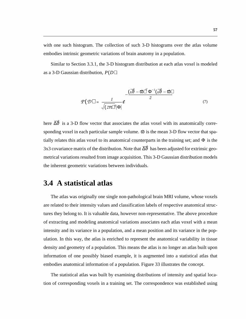
57
with one suchhistogram.The collection of such3-D histogramsover the atlasvolume
embodies intrinsic geometric variations of brain anatomy in a population.
Similar to Section3.3.1,the3-D histogramdistributionat eachatlasvoxel is modeled
as a 3-D Gaussian distribution, :
here is a 3-D flow vectorthat associatesthe atlasvoxel with its anatomicallycorre-
spondingvoxel in eachparticularsamplevolume. is themean3-D flow vectorthatspa-
tially relatesthisatlasvoxel to its anatomicalcounterpartsin thetrainingset;and is the
3x3covariancematrixof thedistribution.Notethat hasbeenadjustedfor extrinsicgeo-
metricalvariationsresultedfrom imageacquisition.This3-D Gaussiandistributionmodels
the inherent geometric variations between individuals.
3.4 A statistical atlas
Theatlaswasoriginally onesinglenon-pathologicalbrainMRI volume,whosevoxels
arerelatedto their intensityvaluesandclassificationlabelsof respectiveanatomicalstruc-
turestheybelongto. It is valuabledata,howevernon-representative.Theaboveprocedure
of extractingandmodelinganatomicalvariationsassociateseachatlasvoxel with a mean
intensityandits variancein a population,anda meanpositionandits variancein thepop-
ulation. In this way, the atlasis enrichedto representthe anatomicalvariability in tissue
densityandgeometryof apopulation.Thismeanstheatlasis no longeranatlasbuilt upon
information of one possiblybiasedexample,it is augmentedinto a statisticalatlasthat
embodies anatomical information of a population. Figure33 illustrates the concept.
Thestatisticalatlaswasbuilt by examiningdistributionsof intensityandspatialloca-
tion of correspondingvoxelsin a trainingset.Thecorrespondencewasestablishedusing
P D( )
P D( ) 1
2π( )3 Φ------------------------------e
∆ϑ ω–( )T Φ 1–∆ϑ ω–( )
2-----------------------------------------------------------------–
= (7)
ϑ∆
ω
Φ
ϑ∆
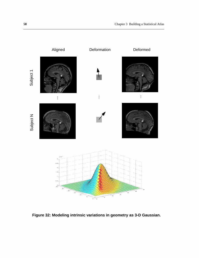
58 Chapter 3 Building a Statistical Atlas
Figure 32: Modeling intrinsic variations in geometry as 3-D Gaussian.
Sub
ject
1S
ubje
ct N
......
DeformedAligned Deformation
...
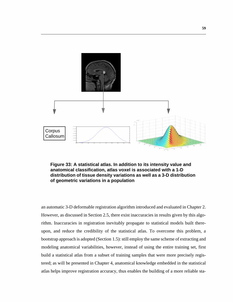
59
an automatic 3-D deformable registration algorithm introduced and evaluated in Chapter 2.
However, as discussed in Section 2.5, there exist inaccuracies in results given by this algo-
rithm. Inaccuracies in registration inevitably propagate to statistical models built there-
upon, and reduce the credibility of the statistical atlas. To overcome this problem, a
bootstrap approach is adopted (Section 1.5): still employ the same scheme of extracting and
modeling anatomical variabilities, however, instead of using the entire training set, first
build a statistical atlas from a subset of training samples that were more precisely regis-
tered; as will be presented in Chapter 4, anatomical knowledge embedded in the statistical
atlas helps improve registration accuracy, thus enables the building of a more reliable sta-
−80 −60 −40 −20 0 20 40 60 80 1000
0.002
0.004
0.006
0.008
0.01
0.012
0.014
Figure 33: A statistical atlas. In addition to its intensity value andanatomical classification, atlas voxel is associated with a 1-Ddistribution of tissue density variations as well as a 3-D distributionof geometric variations in a population
CorpusCallosum
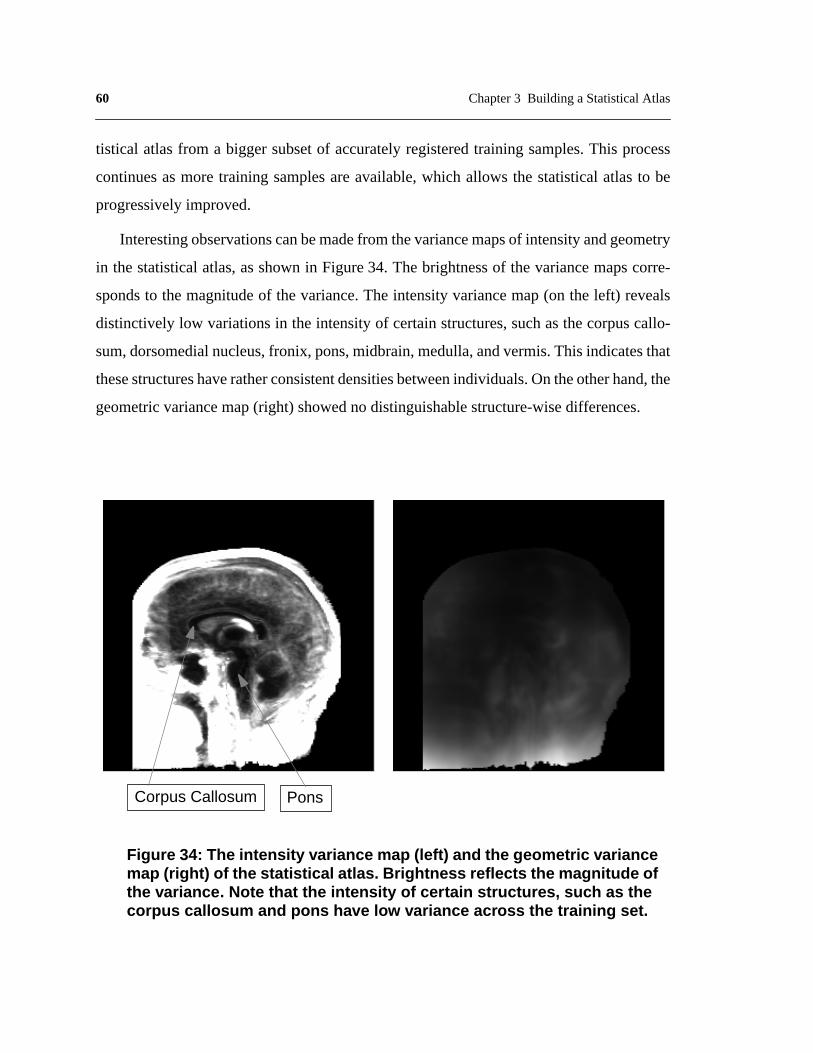
60 Chapter 3 Building a Statistical Atlas
tistical atlas from a bigger subset of accurately registered training samples. This process
continues as more training samples are available, which allows the statistical atlas to be
progressively improved.
Interesting observations can be made from the variance maps of intensity and geometry
in the statistical atlas, as shown in Figure 34. The brightness of the variance maps corre-
sponds to the magnitude of the variance. The intensity variance map (on the left) reveals
distinctively low variations in the intensity of certain structures, such as the corpus callo-
sum, dorsomedial nucleus, fronix, pons, midbrain, medulla, and vermis. This indicates that
these structures have rather consistent densities between individuals. On the other hand, the
geometric variance map (right) showed no distinguishable structure-wise differences.
Figure 34: The intensity variance map (left) and the geometric variancemap (right) of the statistical atlas. Brightness reflects the magnitude ofthe v ariance . Note that the intensity of cer tain structures, suc h as thecorpus callosum and pons ha ve lo w variance acr oss the training set.
PonsCorpus Callosum

61
3.5 Discussion
Theproblemof modelinganatomicalvariability is approachedby augmentinganatlas
basedon a singleexampleinto a statisticalatlasbuilt from a population.Thestatisticsare
gleanedby comparingsamplesfrom a trainingsetin thecommonreferenceframeof the
original atlas,using 3-D deformableregistration.Patternsof anatomicalvariationsare
modeledusingthefirst andsecondorderstatisticsof themeasurements.Otheroptionswere
consideredandinvestigatedduringthedesignprocess,whicharepresentedherefor future
reference.
3.5.1 Population-specific training sets
Thecurrentstatisticalatlaswasbuilt on a trainingsetof non-pathologicalbrainMRI
volumes.Dueto thedifficulty of acquiringsufficientdata,subjectsin this trainingsetare
not stratifiedinto subpopulationsaccordingto age,gender,or anyotherdemographiccri-
teria.However,researchin neurologyhasrevealedthatstructuralchangesdueto growth,
aging,andcertainpsychiatricdiseasesareobservableat bothcellularandgrossanatomic
scales.In thecaseof thecorpuscallosum,it undergoesprofoundchangesin morphology
andcompositionduringbraindevelopment,andthesepatternsaredramaticallyalteredin
psychiatricdiseasessuchasmulti-infarct dementia,schizophrenia,Alzheimer’sDisease,
etc. Therefore,a static representationis ill-suited to determiningthe dynamiceffectsof
developmentanddisease.With theavailabilityof largeimagearchives,population-specific
atlases should be built to encode population variability.
3.5.2 Manual versus automatic classification
It is arguablethatstudyinganatomicalvariationsfrom atrainingsetof expertclassified
datamay producemore precisemodels.However,manuallyclassifyinghigh-resolution
volumetricdataisextremelytime-consuming(it tookanexperteightmonthstoclassify144
structuresin theatlasvolume).Thismakesit difficult if not impossibleto acquireasizable
training set.Moreover,the inherentsubjectivenessand inconsistencyin humanperfor-
62 Chapter 3 Building a Statistical Atlas
mance,betweenpeopleor for thesamepersonovertime,will likewisedecreasethepreci-
sion of models built upon it ([14], Chapter1).
3.5.3 Multiple experts’ opinions
The currentstatisticalatlasencodesanatomicalvariationsof a population.However,
the anatomicalclassificationis still one expert’sopinion, which can be subjectiveand
biased.Combiningdifferentexperts’opinionsin aprobabilisticmannerwill provideamore
impartial classification.
3.5.4 Global versus structure-based models
As discussedin Section3.1,modelsof anatomicalvariationscanbelocal or global.In
this thesis,theprimarygoalof modelinganatomicalvariability is to achieveaccuratereg-
istrationandsegmentationof all brainstructuressimultaneously.Therefore,aglobalmodel
thatencompassesall structuresaswell astheir spatialrelationsandinteractionsis prefera-
ble. Thecurrentstatisticsarevoxel-based,but structureor multi-structurebasedstatistics
can be conveniently modeled and incorporated within the framework.
3.5.5 Choice of method
In modelinggeometricvariationsfrom the trainingset’s3-D deformationflow, other
methodsthan voxel-basedstatisticswere also considered,suchas principal component
analysis(PCA), modalanalysis,andfinite elementsurfacemodel.Thepotentialof using
PCA was further investigated, and presented in Appendix B.
PCA is a morecompactway to representtheaveragegeometryandmajorpatternsof
variations.However,dueto thehighdimensionalityof MRI data,it is currentlyimpractical
to conductPCA on 3-D deformationflow of thewholevolumes.While PCA canbeused
to modelthemeangeometryandmajormodesof variationof individualanatomicalstruc-
tures,critical informationon their relativepositionandinter-structureinteractionis lost.

63
One possible solution was investigated and presented in Appendix B, but it did not promise
to improve registration accuracy over the existing algorithm.
3.6 Chapter summary
This chapter has focused on augmenting the atlas from a non-representative, single
example into a statistical atlas that embodies anatomical variations of a population.
Although there are many applications for a statistical atlas, the major interest of this thesis
is to use it to achieve accurate registration and segmentation, which will be discussed in the
following chapters.

64 Chapter 3 Building a Statistical Atlas
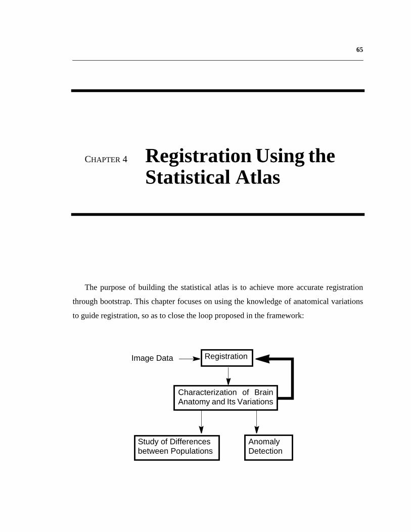
65
CHAPTER 4 Registration Using theStatistical Atlas
The purpose of building the statistical atlas is to achieve more accurate registration
through bootstrap. This chapter focuses on using the knowledge of anatomical variations
to guide registration, so as to close the loop proposed in the framework:
Study of Differencesbetween Populations
AnomalyDetection
Characterization of BrainAnatomy and Its Variations
RegistrationImage Data

66 Chapter 4 Registration Using the Statistical Atlas
4.1 Related Work
Despite much effort on modeling individual variabilities of anatomical structures, few
researchers have reported on using knowledge of anatomical variations to improve regis-
tration. Moghaddam et al. presented a probabilistic similarity measure for direct image
matching based on a Bayesian analysis of image deformations [71]. They modeled varia-
tions in object appearance as probabilistic distributions, and computed a similarity measure
based on the a posteriori probabilities. This approach was applied to 2-D image recognition.
Gee et al. [31] proposed a Bayesian formulation of the image matching problem, and tested
it on 2-D MRI data generated by applying manually defined distortions to real MRI data.
Results on matching image volumes from different individuals are as yet unavailable.
Wang and Staib posed 2-D deformation estimation problem in a maximum a posterori
framework, in which statistical shape model based on corresponding boundary points were
used as prior probabilities [104].
4.2 Registration using the statistical atlas
Similar to the approaches in related work, image registration is formulated within a
Bayesian estimation-theoretic framework: the statistics derived from past observations
specify the relevant prior probability model for the unknown spatial mapping. A Bayesian
framework is well suited to the task of modeling variations in morphology. Because we are
dealing with uncertain quantities, such as noisy data, from which information or decisions
are derived (that must themselves then be uncertain), it is natural to adopt a probabilistic
approach. Second, Bayesian analysis formally embodies the use of prior information that
we have about the problem. In matching, the prior serves to constrain the mappings by
favoring certain configurations, in effect, regularizing the problem. Statistical information
about morphological variability, accumulated over past samples, can be formally intro-
duced into the problem formulation to guide the matching or normalization of future data
sets. Among the many operational advantages of Bayesian analysis, the most relevant to
this work is that the result is a posterior distribution for the unknown mapping, which
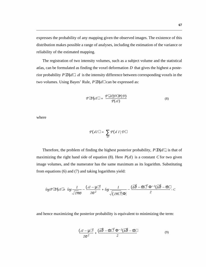
67
expressestheprobabilityof anymappinggiventheobservedimages.Theexistenceof this
distributionmakespossiblearangeof analyses,includingtheestimationof thevarianceor
reliability of the estimated mapping.
Theregistrationof two intensityvolumes,suchasa subjectvolumeandthestatistical
atlas,canbeformulatedasfinding thevoxeldeformation thatgivesthehighestaposte-
rior probability . is theintensitydifferencebetweencorrespondingvoxelsin the
two volumes. Using Bayes’ Rule, can be expressed as:
where
Therefore,theproblemof finding thehighestposteriorprobability, , is thatof
maximizingtheright handsideof equation(8). Here is a constant for two given
imagevolumes,andthe numeratorhasthe samemaximumasits logarithm.Substituting
from equations (6) and (7) and taking logarithms yield:
and hence maximizing the posterior probability is equivalent to minimizing the term:
D
P D Id⟨ | ⟩ Id
P D Id⟨ | ⟩
P D Id⟨ | ⟩ P Id D⟨ | ⟩P D( )P Id( )
--------------------------------------= (8)
P dI( ) P d I D( )D∑=
P D Id⟨ | ⟩
P Id( ) C
P D Id⟨ | ⟩log 12πσ
-----------------log Id µ–( )2
2σ2-------------------------– 1
2π( )3 Φ------------------------------log ∆ϑ ω–( )T Φ 1– ∆ϑ ω–( )
2---------------------------------------------------------------------– C–+=
Id µ–( )2
2σ2------------------------- ∆ϑ ω–( )T Φ 1– ∆ϑ ω–( )
2---------------------------------------------------------------------+ (9)

68 Chapter 4 Registration Using the Statistical Atlas
Gradientdescentis usedto minimizesthetermin (9).The3-D gradient, , ateachstep
of the descent is given by the first order derivative of (9):
where is the3-D imagegradient,which is a functionof thevoxel’s position.Thefirst
termwill shift thecurrentvoxelby movingit in thedirectionthatwill reducethedifference
betweenits currentintensityandits meanintensityacrossall trainingsamples.If thevari-
ancein thisvoxel’sintensitydistributionis large,themagnitudeof thestepalongtheimage
gradientwill bereduced.Thesecondtermwill shift thecurrentvoxelby movingit towards
the meangeometricdeformationof this voxel in the training set. If the varianceof this
voxel’sgeometricdistributionis large,themagnitudeof thestepwill bereduced.Since
and canhavesmallvalues,a stabilizingfactor is addedto andto thediagonalele-
mentsof to regularizethegradient.Theempiricalvalueusedis . The3-D shift
of the voxel is then:
here is a stepsizeconstant.In this way, eachvoxel in the statisticalatlasis guidedto
searchfor acounterpartin thesubject,sotheirmatchis mostprobableaccordingto thesta-
tisticsgatheredfrom a population.3-D Gaussiansmoothingis appliedto thevoxels’ 3-D
displacementsaftereachiterationto smooththedeformation.Thiscompensatesfor thefact
thatthedependencebetweenthedeformationof neighboringvoxelsis not modeledin the
currently voxel-based statistics.
This algorithm differs from the hierarchicaldeformableregistrationalgorithm dis-
cussedin Chapter2 in themeasurementof thegoodnessof thevoxeldeformationflow. In
this method,thegoodnessis theposteriorprobabilityof thecurrentdeformation,which is
maximizedusingprior statisticsgatheredfrom atrainingset;in thepreviousalgorithm,the
badness is theintensitydifferencebetweenspatiallycorrespondingvoxelsin theatlasand
thesubjectvolume,which wasminimizedoverthevolumes.Beforeundergoingdeforma-
∇
∇ Id µ–
σ2----------------- I∇ Φ 1– ∆ϑ ω–( )+= (10)
I∇
σ
Φ σ2
Φ I∇ 1+
δD
δD λ∇–= (11)
λ

69
tion, both algorithmsglobally align the two imagevolumesto eliminateextrinsicvaria-
tions.
4.3 Performance evaluation
To validatethis approach,thealgorithmis appliedto thesametestsetasdescribedin
Section2.4.Experimentsareconductedto examinetheeffectivenessof the intensityand
geometric statistics alone as well as their combined strength.
4.3.1 Registration using the intensity statistics
Theeffectivenessof theintensitystatisticsmodelis testedby assumingaconstantgeo-
metric prior probability. The maximization problem in equation (8) simplifies to:
and equation (10) becomes:
Using this methodto registertheatlaswith the testset,theoverallmislabelledvoxel
ratio is 3.8%.This is a 13.6%errorreductionoverthealgorithmwith no knowledgeguid-
ance, which had an error rate of 4.4% (Section2.4).
4.3.2 Registration using the geometric statistics
In thisexperiment,theeffectivenessof thegeometricstatisticsmodelis assessed,with
theintensitystatisticsassumedto beaconstant.Themaximizationproblemin equation(8)
becomes:
P D Id⟨ | ⟩ P Id D⟨ | ⟩∝
∇ Id µ–
σ2----------------- I∇=
P D dI( ) P D( )∝
70 Chapter 4 Registration Using the Statistical Atlas
and the 3-D gradient at each step is the second term in equation (10):
however, alone is insufficient to determinethe deformation,becauseit ignoresthe
imagesbeingregistered,andforcesthedeformationtowardtheaverage brain.To combine
theprior modelpredictionandtheobserveddata,theinnerproductbetween andimage
gradient is used to obtain a 3-D deformation gradient:
this helpsto balancetheinfluenceof theprior distributionandthefidelity to theobserva-
tions.Whenappliedto registertheatlasto thetestset,thismethodyieldsanoverallmisla-
belled voxel ratio of 4.05%.This is an 8% error reductionover the algorithm with no
knowledge guidance.
4.3.3 Registration using the statistical atlas
Whenbothintensityandgeometricprior distributionsareused,asderivedin equation
(10),registrationbetweentheatlasandthetestsetyieldsanoverallmislabelledvoxel ratio
of 3.6%.This a 18.2%error reductionover thealgorithmusingtheoriginal atlaswith no
knowledgeguidance.Figure35 showsan exampleof improvedregistrationperformance
using the statistical atlas, compared to result given by using the original atlas.
Theseexperimentsshowthatwhile theintensitystatisticsmodelis moreeffectivethan
the geometricone at guiding the deformableregistration,the best registrationresult is
achievedwhentheintensityandgeometricstatisticsmodelsarecombined.Figure36com-
paresregistrationperformanceusingtheoriginal atlas,usingvoxel-basedintensitystatis-
tics only, using voxel-based geometric statistics only, and using the statistical atlas.
Registrationusingthe full statisticalatlastakes35 minutesto register3-D imagesof
256x256x124 voxels on a SGI workstation with four 194 MHz processors.
∇ Φ 1– ∆ϑ ω–( )=
∇
∇
∇̃ ∇∇
----------°I∇I∇
-------------- ∇= (12)

71
4.4 Discussion
In order to build the statistical atlas, each image volume in the training set was warped
to match the atlas. Therefore, the geometric statistics represent the distribution of 3-D dis-
placements from each atlas voxel to voxels in different subject volumes. However, for most
applications, it is preferable to compute the inverse deformation i.e. to warp the atlas to
match the subject volume. In this way, anatomical classifications in the atlas can be cus-
tomized for the particular subject, thus facilitate interesting applications. Unfortunately, the
analytical inverse of the voxel-based 3-D deformation does not exist. One practical solution
is to interpolate the inverse deformation.
Figure 37 gives an 1-D illustration. Assume is one dimension in the atlas, and
is the corresponding dimension in the subject volume. From the statistical atlas, the corre-
spondence from each position on to that on can be computed. What is unknown is
Use Statistical AtlasUse Original Atlas
Figure 35: Registration using the statistical atlas achievesbetter performance than using the original atlas.
ϑa ϑs
ϑa ϑs

72 Chapter 4 Registration Using the Statistical Atlas
the correspondence from each position on to that on . Take a particular position ,
the current hypothesis in gradient descent corresponds it to . However, from the prior
probabilities encoded in the statistical atlas, should correspond to via a displace-
ment . What needs to be determined is the correspondence for that is consistent
with the prior knowledge in the statistical atlas. Assume that the correct correspondence for
is only one small step away from , and that changes between neighboring dis-
placements are linear, we have
Original Atlas Intensity Prior Only Geometric Prior Only Statistical Atlas 0
0.5
1
1.5
2
2.5
3
3.5
4
4.5
% o
f mis
labe
lled
voxe
ls
Figure 36: Error ratios of the test set given by registration using theoriginal atlas, using voxel-based intensity statistics only, using voxel-based geometric statistics only, and using the statistical atlas. Theintensity statistics prior is more effective than the geometric one atguiding registration; the best result is achieved using the statisticalatlas with both intensity and geometric statistics.
ϑs ϑa ϑs2
ϑa1
ϑa1 ϑs1
µ ϑa1( ) ϑs2
ϑs2 ϑaδ ϑa1
ϑs2 ϑa1 ϑaδ µ ϑa1 ϑaδ+( )+ += (13)

73
Take Taylor expansion of , and ignore higher order terms give:
Combining the above two equations gives
In this way, the correspondence for , , is determined:
Empirically,theassumptionsof smallstepandlinearchangein neighboringflows hold
well. More study on neighboring flows will be presented in Chapter5.
4.5 Chapter summary
Thischapterappliesthestatisticalatlasto 3-D deformableregistration.UsingBayesian
formulation,statisticsembeddedin the atlasfunction asprior probabilities.The optimal
deformationmaximizestheposteriorprobability.Thisapproachis evaluatedby registering
thestatisticalatlasto thesametestsetasdescribedin Section2.4.Theoverallerrorrateis
3.6%,which is a18.2%reductionoverthepreviousalgorithm(Section2.4).However,the
currentknowledgemodelis simplyvoxel-basedstatistics,considerationsonneighborhood
context will be discussed in the next chapter.
µ ϑa1 ϑaδ+( )
µ ϑa1 ϑaδ+( ) µ ϑa1( ) µ ϑa1( )∇( ) ϑaδ+= (14)
ϑaδ 1 µ ϑa1( )∇+( ) 1– ϑs2 ϑa1– µ ϑa1( )–( )=
ϑs2 ϑa2
ϑa2 ϑa1 ϑaδ+=

74 Chapter 4 Registration Using the Statistical Atlas
Priorϑs1 ϑa1 µ ϑa1( )+=
Hypothesis
• Small Step• Linear Chang e inNeighboring Flo ws
Interpolate Flowϑs2 ϑa1 ϑaδ µ ϑa1 ϑaδ+( )+ +=
Taylor Expansion
µ ϑa1 ϑaδ+( ) µ ϑa1( ) µ ϑa1( )∇( ) ϑaδ+=
ϑaδ 1 µ ϑa1( )∇+( ) 1– ϑs2 ϑa1– µ ϑa1( )–( )=
ϑs2 ϑa1
ϑa
ϑsϑs1 ϑs2
ϑa1
ϑaδ
µ ϑa1( )
Figure 37: 1-D illustration of interpolating the in verse def ormation
Correspondenceϑa2 ϑa1 ϑaδ+=

75
CHAPTER 5 Model NeighborhoodContext
Currently, anatomical variations between individuals are modeled as voxel-based sta-
tistics. This representation is simple and efficient, as demonstrated in Section 4.3. How-
ever, information on voxel neighborhood context is missing. Figure 38 is a close-up on the
posterior part of corpus callosum in the mid-sagittal plane. 2-D projections of the 3-D
deformation flow are overlaid on top of the intensity image. Note that the deformation flow
is smooth and congruous locally, which means the deformation at each voxel is not com-
pletely independent of its neighbors. Therefore, a more comprehensive model should con-
sider this dependency between neighboring voxels, which will be the focus of this chapter.
5.1 Modeling neighborhood context
A convenient way to model neighborhood dependency is a direct higher dimensional
extension of the voxel-based statistics models. Consider a 3-D neighborhood of NxMxK
centered at an atlas voxel; the distribution of intensity variations of this neighborhood is
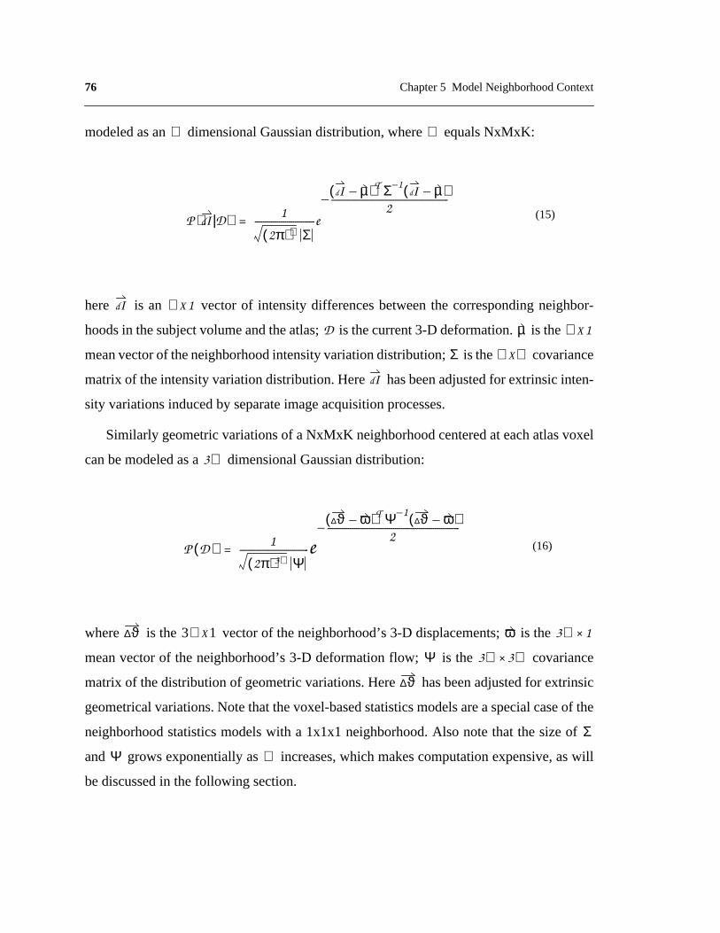
76 Chapter 5 Model Neighborhood Context
modeled as an dimensional Gaussian distribution, where equals NxMxK:
here is an vectorof intensitydifferencesbetweenthe correspondingneighbor-
hoodsin thesubjectvolumeandtheatlas; is thecurrent3-D deformation. is the
meanvectorof theneighborhoodintensityvariationdistribution; is the covariance
matrixof theintensityvariationdistribution.Here hasbeenadjustedfor extrinsicinten-
sity variations induced by separate image acquisition processes.
Similarly geometricvariationsof aNxMxK neighborhoodcenteredateachatlasvoxel
can be modeled as a dimensional Gaussian distribution:
where is the vectorof theneighborhood’s3-D displacements; is the
meanvectorof theneighborhood’s3-D deformationflow; is the covariance
matrixof thedistributionof geometricvariations.Here hasbeenadjustedfor extrinsic
geometricalvariations.Notethatthevoxel-basedstatisticsmodelsareaspecialcaseof the
neighborhoodstatisticsmodelswith a 1x1x1 neighborhood.Also notethat the sizeof
and growsexponentiallyas increases,which makescomputationexpensive,aswill
be discussed in the following section.
ℜ ℜ
P Id D⟨ | ⟩ 1
2π( )ℜ Σ-------------------------------e
Id µ–( )T Σ 1– Id µ–( )2
-----------------------------------------------------------–
= (15)
Id ℜX1
D µ ℜX1
Σ ℜXℜ
Id
3ℜ
P D( ) 1
2π( )3ℜ Ψ-----------------------------------e
∆ϑ ω–( )T Ψ 1–∆ϑ ω–( )
2-------------------------------------------------------------------–
= (16)
∆ϑ 3ℜX1 ω 3ℜ 1×
Ψ 3ℜ 3ℜ×
∆ϑ
Σ
Ψ ℜ
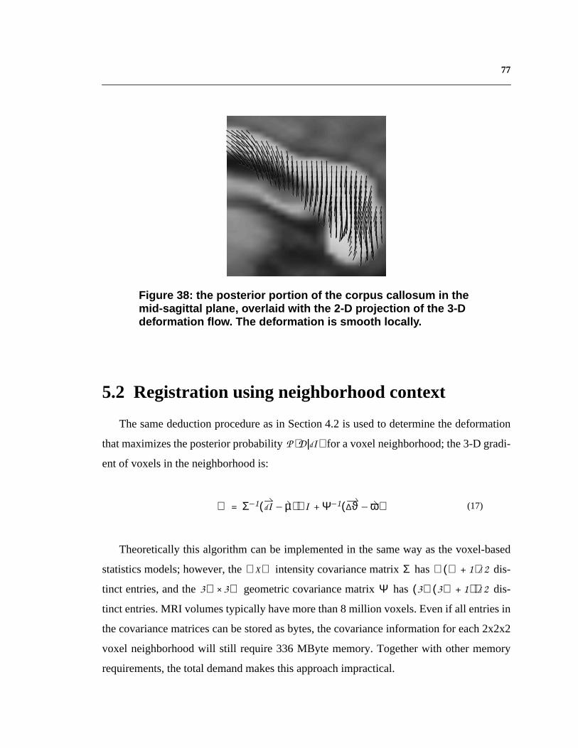
77
5.2 Registration using neighborhood context
Thesamedeductionprocedureasin Section4.2 is usedto determinethedeformation
thatmaximizestheposteriorprobability for avoxelneighborhood;the3-D gradi-
ent of voxels in the neighborhood is:
Theoreticallythis algorithmcanbe implementedin thesameway asthevoxel-based
statisticsmodels;however,the intensitycovariancematrix has dis-
tinct entries,andthe geometriccovariancematrix has dis-
tinct entries.MRI volumestypically havemorethan8 million voxels.Evenif all entriesin
thecovariancematricescanbestoredasbytes,thecovarianceinformationfor each2x2x2
voxel neighborhoodwill still require336 MByte memory.Togetherwith othermemory
requirements, the total demand makes this approach impractical.
Figure 38: the posterior por tion of the corpus callosum in themid-sa gittal plane , overlaid with the 2-D pr ojection of the 3-Ddeformation flo w. The def ormation is smooth locall y.
P D Id⟨ | ⟩
∇ Σ 1– Id µ–( ) I∇ Ψ 1– ∆ϑ ω–( )+= (17)
ℜXℜ Σ ℜ ℜ 1+( ) 2⁄
3ℜ 3ℜ× Ψ 3ℜ 3ℜ 1+( )( ) 2⁄

78 Chapter 5 Model Neighborhood Context
To simplify theproblem,only the interactionsbetweenimmediateneighborsarecon-
sidered.Insteadof storinginteractionsbetweenimmediateneighbors,theyarecomputed
on thefly. Thevoxel-neighborinteractionsareestimatedusingthegoodness of theneigh-
bors’ currentmatchaccordingto their respectiveprior distributions.Figure39 illustrates
the idea:thegoal is to find a matchfor theblackvoxel in thesubject;however,whenno
neighborhoodcontextis considered,thereis ambiguityasto whichblackvoxel in theatlas
it shouldmatchto. But whenconsideringthegoodnessof how well theneighborsof the
blackvoxel in thesubjectmatchwith their counterpartsin theatlas,it is clearwhich atlas
voxel it should match to.
Using a weighted-windowmatchingapproach,the goodness is weightedby the dis-
tancebetweenthecurrentvoxelunderinvestigationandtheparticularneighbor.Therefore,
for avoxelneighborhood , the3-D gradientdeterminedusingneighborhoodcontextis a
direct extension of equation (10):
Atlas Subject
?Figure 39: Registration using neighborhood context
ℵ
∇ w ijkId µ–
σ2----------------- I∇
ijki j k, ,
∑ w ijk Φ 1– ∆ϑ ω–( )[ ]ijki j k, ,∑+= ijk ℵŒ (18)

79
5.3 Performance evaluation
The algorithm is evaluated by registering the atlas to the same test set as in Section 4.3.
The size of the voxel neighborhood used is 3x3x3. Weights of neighboring voxels are
inversely proportional to their distance from the voxel under examination. Empirical num-
bers used are 0.01 for 8 farthest neighbors, 0.014 for 12 intermediate neighbors, and 0.017
for 6 closest neighbors. Experiments showed that as long as major weight is put on the cen-
tral voxel, registration results are not sensitive to the particular numbers. Registration using
neighborhood context achieves an overall error ratio of 2.9%. This is a 34% error reduction
over the algorithm with no knowledge guidance, and a 19.4% error reduction over registra-
tion using the statistical atlas. Figure 40 shows an example of better registration achieved
by using neighborhood context, and Figure 41 compares examples of segmentation given
by the algorithm, and the respective segmentation given by experts.
Use Neighborhood Context Use Voxel-based Statistics
Figure 40: Better registration is achievedby considering neighborhood context.

80 Chapter 5 Model Neighborhood Context
This weighted window matching approach yields better results than using voxel-based
statistics without increasing memory demand, as compared in Figure 42. However, it is
much more computationally expensive. To register 3-D images of 256x256x124 voxels on
a SGI workstation with four 194 MHz processors will take 57 minutes. Appendix C com-
pares the expert segmentation and the computed segmentation of the corpus callosum in the
mid-sagittal plane of each of the 40 test cases. The images are binary, with the corpus cal-
losum shown at intensity 140, and the rest shown as zero intensity background. Error ratios
given by the weighted window matching approach are listed under respective computed
segmentations.
Expert Segmentation Automatic Segmentation
Figure 41: Examples of automatic segmentation comparedto their respective expert segmentation
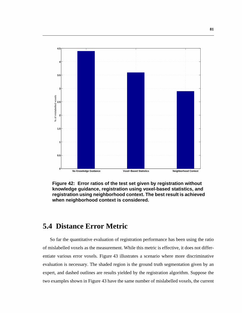
81
5.4 Distance Error Metric
So far the quantitative evaluation of registration performance has been using the ratio
of mislabelled voxels as the measurement. While this metric is effective, it does not differ-
entiate various error voxels. Figure 43 illustrates a scenario where more discriminative
evaluation is necessary. The shaded region is the ground truth segmentation given by an
expert, and dashed outlines are results yielded by the registration algorithm. Suppose the
two examples shown in Figure 43 have the same number of mislabelled voxels, the current
No Knowledge Guidance Voxel−Based Statistics Neighborhood Context 0
0.5
1
1.5
2
2.5
3
3.5
4
4.5
% o
f m
isla
be
lled
vo
xels
Figure 42: Error ratios of the test set given by registration withoutknowledge guidance, registration using voxel-based statistics, andregistration using neighborhood context. The best result is achievedwhen neighborhood context is considered.

82 Chapter 5 Model Neighborhood Context
error metric will give them the same evaluation. However, errors in these two results are of
different significance. For the example shown on the left, its error voxels occur close to the
boundary of the ground truth segmentation; whereas for the result on the right, many of its
error voxels stray considerably away from the ground truth segmentation. Therefore, in
terms of segmentation quality, the example on the left is better than the one on the right.
A more discerning measurement is the distance between each boundary voxel of the
computed segmentation and the closest boundary voxel of the ground truth segmentation.
Under this metric, error voxels that are far away from the true boundary will be penalized
more than error voxels that occur close by the ground truth., i.e. it de-emphasizes errors that
are near the true boundary. This is especially advantageous considering boundary voxels
are of higher uncertainty even in expert segmentation.
Using the distance error metric to evaluate the registration performance of the weighted
window matching approach, the mean distance of error voxels for the test set is 1.535 mm,
and the standard deviation is 0.762 mm. Figure 44 shows histogram distributions of dis-
tance measurements of boundary voxels. The histogram at the top includes the correct
boundary voxels, i.e. the voxels that lie on the true boundary. Because the number of cor-
rect boundary voxels is orders of magnitudes larger than the number of erroneous boundary
voxels, it is impossible to visualize the distribution of distance measurements of error vox-
Figure 43: A senario that demands more discriminative evaluation. The shadedregion is the ground truth segmentation given by an expert, and dashed outlines areresults yielded by the registration algorithm. Suppose the two examples have thesame number of mislabelled voxels, using the ratio of mislabelled voxels will givethem the same evaluation. However,in terms of segmentation quality, the exampleshown on the left is better than the one shown on the right.

83
els. Therefore, the correct boundary voxels are excluded in the histogram on the bottom,
thus allowing visualization of the distribution of error voxels in terms of the distance met-
ric. The vertical axis of this histogram is at a scale of the top one. Note that most
error voxels are within 2 mm from true boundaries, with few voxels being farther than 4
mm away, and no voxels are beyond 9.4 mm distance. Considering the average length of
the corpus callosum is around 100 mm (4 inches), this level of accuracy is satisfactory.
5.5 Discussion
Markov Random Field (MRF) has been used in computer vision to model smoothness
as well as different textures. Typical solvers for MRFs include Gibbs sampling [35], the
Metropolis algorithm [68], Iterated Conditional Modes (ICM) [5], and Mean-Field (MF)
methods [34]. Kapur et al. used a discrete vector valued Markov Random Field model as a
regularizing prior in a Bayesian classification algorithm to minimize the effect of salt-and-
pepper noise. They presented preliminary results on segmentation of white matter, gray
matter, fluid, and fat in brain MRIs [49]. The possibility of using MRF to model neighbor-
hood context was investigated. However, the dimensionality of volumetric data and the 3-
D nature of deformation fields have so far made the memory demand prohibitive even for
the 1-order model. With computer memory more readily available, this is an alternative
worth studying.
5.6 Chapter summary
This chapter discussed the modeling of neighborhood context in the statistical priors,
and an implementation of applying such knowledge to guide registration. Quantitative
evaluation demonstrated better performance than using just voxel-based statistics. A new
error metric based on distances between boundary voxels of the computed segmentation
and the ground truth is introduced, and employed to assess the registration performance
using neighborhood context.
7 9000⁄
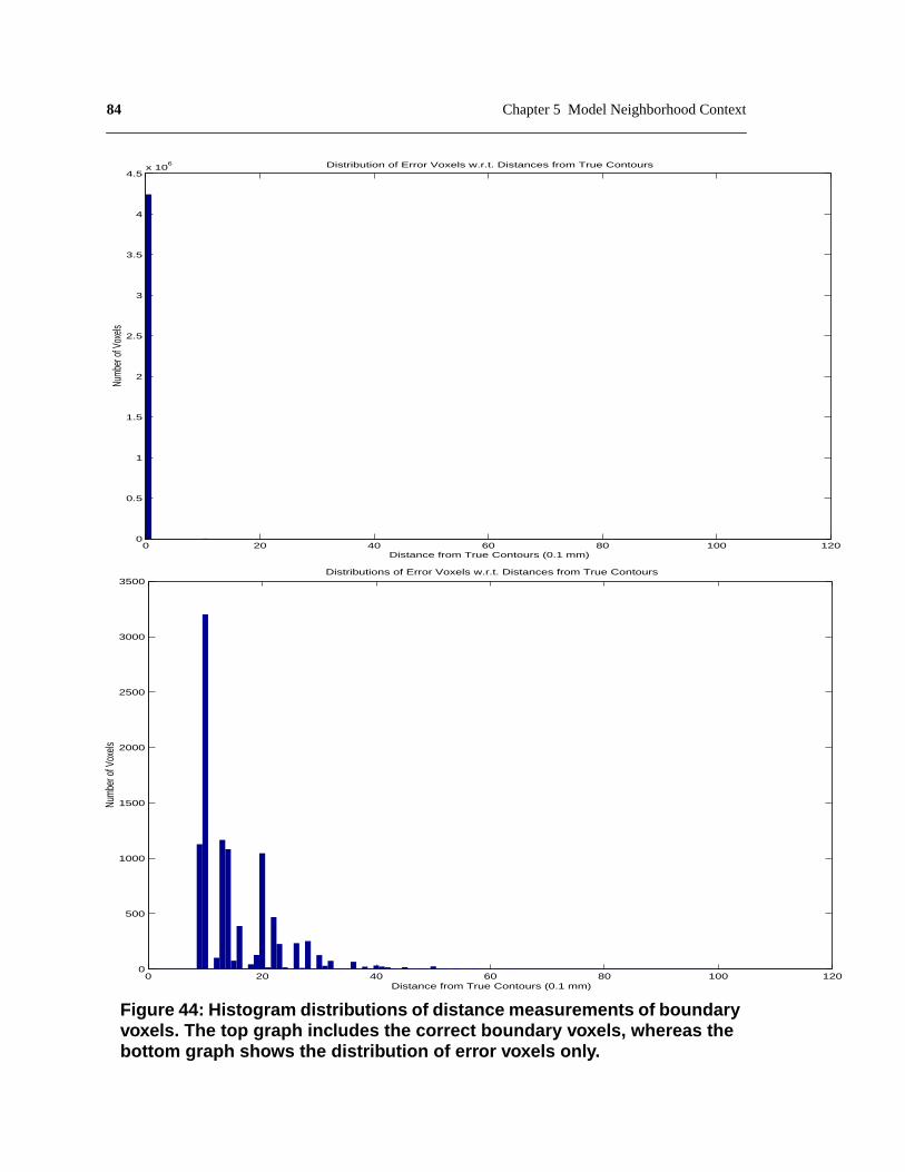
84 Chapter 5 Model Neighborhood Context
0 20 40 60 80 100 1200
500
1000
1500
2000
2500
3000
3500
Distance from True Contours (0.1 mm)
Num
ber o
f Vox
els
Distributions of Error Voxels w.r.t. Distances from True Contours
Figure 44: Histogram distributions of distance measurements of boundaryvoxels. The top graph includes the correct boundary voxels, whereas thebottom graph shows the distribution of error voxels only.
0 20 40 60 80 100 1200
0.5
1
1.5
2
2.5
3
3.5
4
4.5x 10
6
Distance from True Contours (0.1 mm)
Numb
er of
Vox
els
Distribution of Error Voxels w.r.t. Distances from True Contours

85
CHAPTER 6 ImplementationDetails
Several issues in the implementation are crucial to robust and efficient performance.
They apply to both the algorithm using the statistical atlas, and the earlier method without
knowledge guidance. This chapter will discuss them in detail.
6.1 Background Separation
Since the algorithms do not require prior segmentation or feature extraction, each voxel
in the image data is given equal weight in the registration. However, there is often back-
ground noise in the data, which necessitates background separation to ensure only relevant
voxels contribute to the registration process.
A thresholding method is applied to eliminate dim background noise. The threshold is
automatically selected as the first valley of the intensity histogram of the 3-D image, after
it is smoothed using a Gaussian filter (the Gaussian kernel used is of size 7). This produces
a binary image volume with the background intensity set to zero.

86 Chapter 6 Implementation Details
Apart from dim background noise, there also exists bright outliers that have similar
intensities as certain anatomical structures. Since the region containing the head volume is
connected, a connected-component algorithm is applied to the thresholded binary image
volume, and the largest connected component is selected. Any holes caused by dark regions
inside the head volume are filled in. The result is a binary image volume with only voxels
inside the connected component being above zero intensity. This binary volume functions
as a mask to ensure only voxels within the head volume are considered in later processing.
6.2 Adaptive Multi-resolution Processing
Multi-resolution processing has been extensively used in computer vision algorithms,
such as stereo matching and motion estimation. This approach first solves the matching
problem on smaller, lower-resolution data, use the result to initialize higher-resolution esti-
mates, and refine it using details present at the higher resolutions. Its advantage includes
increased computation efficiency, as well as the ability to escape from local minima by first
focusing on global patterns.
MRI volumes are high dimensional data, which makes efficient processing imperative.
The current registration algorithm uses two strands of adaptable multi-resolution process-
ing: one is an image pyramid, the other is a control grid pyramid (in smooth deformation).
Sizes of MRI volumes vary depending on the number of slices. Among the over two hun-
dred MRIs processed by the registration algorithm, the number of slices ranges from 7 to
256. To make the multi-resolution scheme adaptive to different volume sizes, the minimum
number of slices in the subsampled image volumes and the control grid cells are enforced.
The current empirical number is 30 slices for image volumes, and 15 slices for each control
grid cell. This ensures the subsampled volumes and the control grid cells to contain suffi-
cient image information. In the image pyramid, each level has half the resolution of the next
higher level; in the control grid pyramid, the numbers of control points along x, y, and z
increase from 2 at an interval of 1 at each higher lever. For image data so far examined, the

87
highest image pyramid has 3 levels, and the highest control grid pyramid has 7x7x7 control
points.
6.3 Random Initialization
For the ease of application, the algorithms are fully automated. Global Alignment, the
first step of registration, is initiated by trying many random similarity transformations and
picking the one which gives the minimum SSD [74].
Because brain MRI volumes are not taken in a completely random manner, it is efficient
to limit the infinite choices to those that are possible. Since the registration between the
atlas and different subjects is of particular interest, the coordinate frame of one volume, the
atlas, is thus fixed. There are three principal axes along which brain MRIs are taken
(Section 1.4.1), which gives six possible gross orientations of the volumes. For initializa-
tion, it is sufficient to limit the possible rotations from the atlas to these six orientations. As
for translation and scaling, possible transformations are randomly sampled at small inter-
vals within empirical ranges. Currently, random initialization is conducted on images vol-
umes at the coarsest level of the image pyramid. The range for translation is [-8, 8] voxels
along each X-Y-Z dimension, the range for uniform 3-D scaling is [0.9, 1,1]. The number
of random translation and scaling tried for each rotation angle is 300.
6.4 Stochastic Sampling
To further improve algorithm efficiency, not every voxel is processed during the opti-
mization in global alignment and smooth deformation. Instead, a random set of voxels is
sampled at each iteration of the optimization processes. This method is valid because the
optimization processes are over-constrained, i.e. the number of voxels is orders of magni-
tudes greater than the number of parameters to be optimized. It is not necessary to involve
each voxel to solve for the parameters. Moreover, the stochastic nature of the sampling
helps the optimization processes to escape from local minima [103]. In the current imple-
mentation, the percentage of voxels sampled is 1%. For fine-tuning deformation, it has 3

88 Chapter 6 Implementation Details
times as many parameters as the number of voxels, i.e. the problem is highly undercon-
strained, therefore stochastic sampling is not appropriate.
6.5 Parallel Processing
In the registration algorithms developed in this thesis, the computation for each voxel
is identical. Therefore, the process is voxel-wise parallelizable. To reduce overhead, paral-
lel processing is employed at a higher level than the voxel representation. During the
random initialization of global alignment, each combination of transformation parameters
is examined in parallel; during smooth deformation, each control grid cell is processed in
parallel; whereas in fine-tuning deformation, each slice of the image volume is processed
in parallel.

89
CHAPTER 7 Quantitative Studyof the Anatomy
A quantitative study of anatomical structures brings broad prospects to medical
research. It allows measurement of the range of normal variation, and the detection of
abnormalities. Statistics on anatomy and pathologies can help express expert knowledge so
as to enhance medical education. Furthermore, quantitative description of medical image
content will facilitate efficient retrieval in the ever increasing medical databases.
Imaging techniques such as computed tomography and MRI have made it possible to
make non-invasive measurements of anatomical structures. However, traditional mor-
phometry or volumetry (i.e. the measurement of substructural volumes), has been per-
formed manually or semi-automatically. These methods are limited by relatively high error
and low repeatability attributable to the subjective assessment of substructure boundaries
required for manual outlining. However, the magnitude of the volume changes in diseases
such as neurological and psychiatric disorders may be small relative to the error associated
with these measurement techniques. Also, manual operations are tedious and time-consum-
ing, which hampers study of statistically significant data sets.
90 Chapter 7 Quantitative Study of the Anatomy
Major sourcesof errorin manualmeasurementof anatomicalvolumes,in orderof mag-
nitude,comefrom (a) subjectvariability, (b) theobserver,(c) themethodof volumeesti-
mation from the digital image,(d) voxel representation,and (e) the imager.Automatic
algorithmscanhelpreducethesecondandthird sourcesof errorlistedabove.Forexample,
it wasreportedthatusinginteractivethresholdingmethods,expertobserverscouldlearnto
measureanatomicalstructureswith a precisionof about2%; i.e. with practicea single
personcould learnto measurestructuressuchasgreyandwhite matterrepeatedlyon the
samebrain imagewithin that degreeof consistency.However,the sameobserverspro-
ducedmeasurementsthatdifferedbetweenobserversby 15%[41]. Similar intra-andinter-
operatorreliability of 5-20%wasalsomentionedin [70]. Sincea long-termclinical study
cannotdependontheavailabilityof thesameobserverthroughoutthestudy,amoreobjec-
tive automaticalgorithmwith comparableaccuracyis advantageous.Besides,characteriza-
tion of subtleanatomicaberrations,suchashavebeenfound in schizophrenia,requires
quantifyinglocal variability acrosssubjects.This requirementmakeshigh dimensionality
of thetransformationson thecoordinatesystemsessential,which canbereadilyprovided
by automaticalgorithmsthat allow local deformations.In addition, the efficiency of an
automaticalgorithmallows the studyof largedatasets,which is basicto soundconclu-
sions.Furthermore,it hasbeenthecasein this field thatdifferent researchgroupscollect
separatedatasets,andusedifferentoperatorsor semi-automatictoolsto analyzethedata.
Althoughtheyhavehadconflictingconclusions,it hasbeenhardto reproduceor cross-val-
idate eachother’s results.The performanceconsistencyof automaticalgorithmsmakes
cross-examinationpossible.Thischapterwill discusstheapplicationof theaforementioned
registration algorithm to quantitative study of the anatomy:
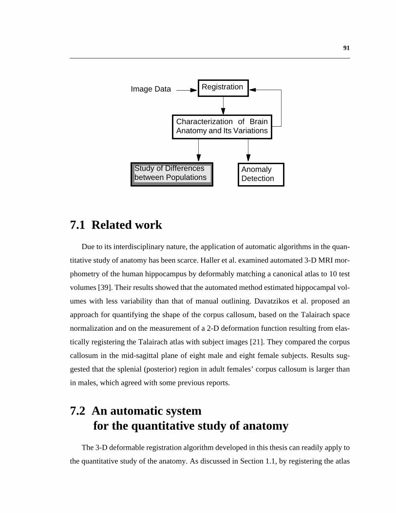
91
7.1 Related work
Dueto its interdisciplinarynature,theapplicationof automaticalgorithmsin thequan-
titativestudyof anatomyhasbeenscarce.Halleretal. examinedautomated3-D MRI mor-
phometryof thehumanhippocampusby deformablymatchinga canonicalatlasto 10 test
volumes[39]. Theirresultsshowedthattheautomatedmethodestimatedhippocampalvol-
umeswith lessvariability than that of manualoutlining. Davatzikoset al. proposedan
approachfor quantifyingtheshapeof thecorpuscallosum,basedon theTalairachspace
normalizationandon themeasurementof a 2-D deformationfunctionresultingfrom elas-
tically registeringtheTalairachatlaswith subjectimages[21]. Theycomparedthecorpus
callosumin the mid-sagittalplaneof eight maleandeight femalesubjects.Resultssug-
gestedthat thesplenial(posterior)regionin adult females’corpuscallosumis largerthan
in males, which agreed with some previous reports.
7.2 An automatic systemfor the quantitative study of anatomy
The3-D deformableregistrationalgorithmdevelopedin this thesiscanreadilyapplyto
thequantitativestudyof theanatomy.As discussedin Section1.1,by registeringtheatlas
Study of Differencesbetween Populations
AnomalyDetection
Characterization of BrainAnatomy and Its Variations
RegistrationImage Data

92 Chapter 7 Quantitative Study of the Anatomy
with a particularsubject’simagevolume,theanatomicalclassificationin theatlascanbe
customizedfor the subject,thereforethe 3-D segmentationof the subject’sanatomical
structures(Figure3). Oncethesegmentationis acquired,quantitativestudyonthesizeand
shape of anatomical structures can be conducted.
In orderto investigateanddemonstratethe feasibility of suchapproach,a convenient
interfacehasbeendevelopedfor quantitativelyexaminingbrain anatomy,as shownin
Figure45.Theleft imageis onesliceof a subject’sT1-weightedMRI volume,andon the
right is thecorrespondingsegmentationautomaticallycustomizedfrom theatlas.Theseg-
mentationis color-codedto representdifferentanatomicalstructures.To studyanystruc-
ture, the user simply clicks on it, and the systeminstantly overlaysthe segmentation
outline(s)on theintensitydata.Thenameof thestructureandseveralmeasurementssuch
asits volumeandaveragedensityareautomaticallycomputedfor illustration.For struc-
tureshavingsymmetriccounterparts,measurementsof theparallelarealsodisplayed.The
slide bar in the left bottomallows the userto examinethe 3-D volume.The underlining
computerlanguagesof this interfaceareC/C++andTcl/Tk, whicharecommonlyavailable
on SGI Irix andSUN Solarisplatforms.For applicationslooking at largepopulations,the
automaticatlas-subjectregistration,customizationof anatomicalsegmentation,andquan-
titative analysis can be readily pipelined.
7.3 Feasibility study
In orderto provethepotentialof automaticquantitativeanalysisof theanatomy,andto
testits acceptabilityto medicalprofessionals,severalcollaborativestudyhavebeencon-
ducted with research groups in medical institutions.
7.3.1 Lateral Ventricles and Schizophrenia
Eversincetheevolutionof theconceptof theschizophrenicillness,it hasbeenargued
that at leastsomepatientsmay havea deteriorativeprocessat work. However,studies
examiningtheprogressionof brainstructuralalterationsin schizophreniahaveled to con-

93
flicting results. Some researchers have found accumulating evidence for abnormalities in
brain structure in adults with schizophrenia, such as lateral ventricular enlargement[24],
[81], whereas some other researchers contend that no substantial differences are seen in
their studies [3], [85]. Researchers at Western Psychiatric Institute and Clinic of the Uni-
versity of Pittsburgh Medical Center have been studying the possible structural and func-
tional changes in schizophrenic patients [51]. However, so far their experiments employ
human operators using semi-automatic tools to acquire anatomical segmentation.
Figure 45: An interface sho wing one slice of a subject’ s data(left), and its automaticall y computed anatomical segmentation(right). When the user selects a structure , its segmentationoutline is o verlaid on the intensity data. The structure’ s nameand se veral measurements are automaticall y displa yed.

94 Chapter 7 Quantitative Study of the Anatomy
Basedon mutualinterestin automaticquantitativeanalysis,segmentationof theright
lateralventriclein nineschizophrenicsandtwelvenormalcontrolswereconductedbothby
theiroperatorsandtheautomaticalgorithm.Histogramsof respectivevolumetricmeasure-
mentgivenby bothmethodsarecomparedin Figure46.Thetop row showsresultsgiven
by theiroperators,with theleft histogramfor normalcontrols,andtheright onefor schizo-
phrenics;thebottomrow givescorrespondingresultsfrom theautomaticanalysis.Despite
asystematictendencyof largervolumesestimatedby theautomaticalgorithm,resultsfrom
thesetwo methodsarehighly correlated(Pearson’scorrelationcoefficient= 0.95).Both
seem to suggest lateral ventricular enlargement in schizophrenics.
7.3.2 Corpus Callosum and Female Alcoholics
Thecorpuscallosumis themainfiber tractconnectingthetwo brainhemispheres,con-
sistingof approximately200-350million fibers in man.Surgicaltransectionof thecallo-
sumin humansprovidesevidencethat it functionsto communicateperceptual,cognitive,
mnemonic,learnedandvolitional informationbetweenthetwo brainhemispheres.Given
theimportanceof sensory,motor,andcognitivecallosalrelaybetweenbrainhemispheres,
this anatomicregionhasbeena focusof studiesexaminingstructuralandfunctionalneu-
ropathology[97]. In disease,effectsoncallosalstructureareobservableatbothcellularand
grossanatomicscales.However,intensecontroversyexistsonthequestionof whetherdif-
ferent callosal regions undergo selective changes in certain diseases.
ResearchersatNationalInstituteonAlcohol AbuseandAlcoholism,NationalInstitute
of Health,havebeeninvestigatinggenderdifferencesin alcoholism-relatedbrainatrophy.
They examinemid-sagittalMRI scansfrom of similarly agedalcoholicwomenandmen
andnormalcontrols,andmeasurethecross-sectionalareaof thecorpuscallosumto exam-
ine braindamage.Unlike otherinvestigatorswho foundthatalcoholicwomenhaveequal
[45], [64] or evensmaller[56] ventriclesthanalcoholicmen,theyobservedthatthecorpus
callosumareawassignificantlysmaller(which leadsto largerventricles)amongalcoholic
womenthannonalcoholicwomenor alcoholicmen.Theseresultssuggestanincreasedsen-

95
3 6 9 12 15 180
10
20
30
40
50
60
70
80
90
100
% of
Test
Case
s
Right Lateral Ventricle (cm3)
Normal
3 6 9 12 15 180
10
20
30
40
50
60
70
80
90
100
% of
Test
Case
s
Right Lateral Ventricle (cm3)
Schizorphrenia
3 6 9 12 15 180
10
20
30
40
50
60
70
80
90
100
% of
Test
Case
s
Right Lateral Ventricle (cm3)
Normal
3 6 9 12 15 180
10
20
30
40
50
60
70
80
90
100
% of
Test
Case
s
Right Lateral Ventricle (cm3)
Schizorphrenia
Figure 46: Histograms of right lateral ventricle volumes of normalcontrols and schizophrenics, resulted from manual estimation (top)and automatic analysis (bottom). High correlation is observed
UP
MC
Researchers
Autom
atic Algorithm
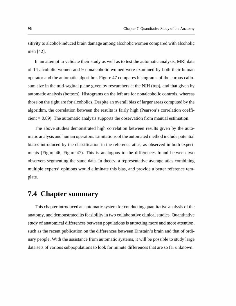
96 Chapter 7 Quantitative Study of the Anatomy
sitivity to alcohol-inducedbraindamageamongalcoholicwomencomparedwith alcoholic
men [42].
In anattemptto validatetheir studyaswell asto testtheautomaticanalysis,MRI data
of 14 alcoholicwomenand9 nonalcoholicwomenwereexaminedby both their human
operatorandtheautomaticalgorithm.Figure47 compareshistogramsof thecorpuscallo-
sumsizein themid-sagittalplanegivenby researchersat theNIH (top),andthatgivenby
automaticanalysis(bottom).Histogramson theleft arefor nonalcoholiccontrols,whereas
thoseontheright arefor alcoholics.Despiteanoverallbiasof largerareascomputedby the
algorithm,thecorrelationbetweenthe resultsis fairly high (Pearson’scorrelationcoeffi-
cient = 0.89). The automatic analysis supports the observation from manual estimation.
The abovestudiesdemonstratedhigh correlationbetweenresultsgiven by the auto-
maticanalysisandhumanoperators.Limitationsof theautomatedmethodincludepotential
biasesintroducedby the classificationin the referenceatlas,asobservedin both experi-
ments(Figure46, Figure47). This is analogousto the differencesfound betweentwo
observerssegmentingthe samedata.In theory,a representativeaverageatlascombining
multiple experts’opinionswould eliminatethis bias,andprovidea betterreferencetem-
plate.
7.4 Chapter summary
Thischapterintroducedanautomaticsystemfor conductingquantitativeanalysisof the
anatomy,anddemonstratedits feasibility in two collaborativeclinical studies.Quantitative
studyof anatomicaldifferencesbetweenpopulationsis attractingmoreandmoreattention,
suchastherecentpublicationon thedifferencesbetweenEinstain’sbrainandthatof ordi-
narypeople.With theassistancefrom automaticsystems,it will bepossibleto studylarge
datasetsof varioussubpopulationsto look for minutedifferencesthataresofar unknown.
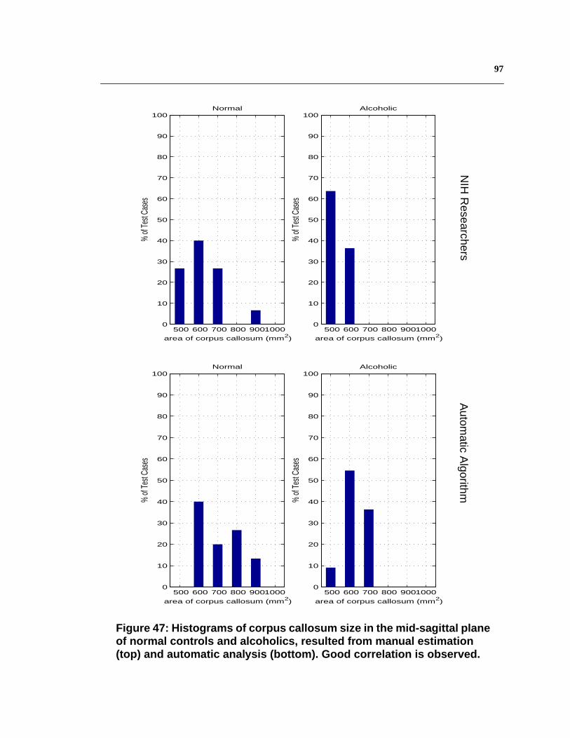
97
500 600 700 800 90010000
10
20
30
40
50
60
70
80
90
100
% of
Test
Case
s
area of corpus callosum (mm2)
Normal
500 600 700 800 90010000
10
20
30
40
50
60
70
80
90
100
% of
Test
Case
s
area of corpus callosum (mm2)
Alcoholic
500 600 700 800 90010000
10
20
30
40
50
60
70
80
90
100
% of
Test
Case
s
area of corpus callosum (mm2)
Normal
500 600 700 800 90010000
10
20
30
40
50
60
70
80
90
100
% of
Test
Case
s
area of corpus callosum (mm2)
Alcoholic
Figure 47: Histograms of corpus callosum size in the mid-sagittal planeof normal controls and alcoholics, resulted from manual estimation(top) and automatic analysis (bottom). Good correlation is observed.
NIH
Researchers
Autom
atic Algorithm

98 Chapter 7 Quantitative Study of the Anatomy
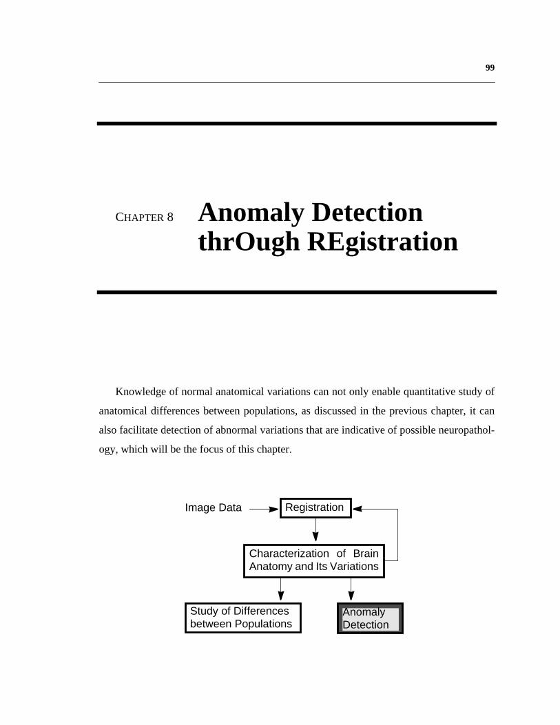
99
CHAPTER 8 Anomaly DetectionthrOugh REgistration
Knowledge of normal anatomical variations can not only enable quantitative study of
anatomical differences between populations, as discussed in the previous chapter, it can
also facilitate detection of abnormal variations that are indicative of possible neuropathol-
ogy, which will be the focus of this chapter.
Study of Differencesbetween Populations
AnomalyDetection
Characterization of BrainAnatomy and Its Variations
RegistrationImage Data

100 Chapter 8 Anomaly Detection thrOugh REgistration
8.1 Related work
Many researchershaveapproachedautomaticpathologydetectionthroughsegmenta-
tion,usingmethodssuchasneuralnetworks[54], automaticsegmentationusinga3-D geo-
metric brain tissueprobability model [48], and spatially weightedK-meanshistogram-
based clustering [61].
A differentresearchavenueis usingregistrationto detectabnormalities.Warfieldetal.
developedanelasticmatchingalgorithmthatwarpsa referencedatasetcontaininginfor-
mationaboutthe locationof the grey matterinto the approximateshapeof the patient’s
brain. White matterandwhite matterlesionswere thensegmentedwithout interference
fromgreymatter,usingatwoclassminimumdistanceclassifier[105].Experimentsonseg-
mentingmultiple sclerosisin sixteenpatientswerepromising.Kyriacou andDavatzikos
studiedfinite elementanalysisto simulatesoft tissuedeformationin the braincausedby
tumorgrowth,andtestedon 2-D elasticregistrationof a standardbrainatlasto simulated
dataandonetumor-bearingimage[57]. Martin et al. proposeda methodto separateout
importantfrom unimportantshapevariationacrossaclassof objects,soasto quantitatively
describepathologicalshapevariations.By modelingthe brain’s elasticproperties,they
wereableto compensatefor someof thenon-pathologicalmodesof shapevariation,and
characterizemodesof variationthatareindicativeof neuropathology[66]. Thompsonetal.
discussedtrackingtumor growth rateby rigidly transformingsubjectdatainto Talairach
stereotaxicspace,andaligninga population-basedprobabilistictissuemapto thesubject
data.A Gaussianmixturedistributionreflectingtheintensitiesof specifictissueclassesat
eachtime-point in the scanserieswas determined,and tissuetypeswere differentiated
using a nearest neighbor algorithm [98].
8.2 Symmetry versus asymmetry
Thereare many typesof neuropathology,of particular interestare pathologiesthat
affectthestructuralsymmetry.Theorganizationalschemeof manyanimalspeciesis based

101
onbilateralsymmetry:someorgansappearin pairsin thebody,“symmetrical”with respect
to the mid-plane;otherorgansareplacednearthe mid-planeandarealsoapproximately
symmetrical.This symmetryis rathergeneralfor thehumanhead,includingthebrainand
its two hemispheres.Oneexampleis shownin the left of Figure48. Thereis approximate
symmetry about the central line.
On theotherhand, symmetricalanatomicalstructuresaresometimesalsoasymmetric,
which meanseachof thetwo organsin a pair canpresenta specializationandthereforea
slightly differentmorphology.For thehumanbrain,somenormalfunctionalasymmetries
are well known, which translateinto morphologicalasymmetries.Furthermore,certain
pathologiescausemass effect, which forcesnearbystructuresto shift from their normal
positions and incur abnormalasymmetry,as shown in the exampleon the right of
Figure48.
LateralVentricles
Figure 48: The corresponding cross-sections of anormal and a pathological brain. The symmetry inthe normal brain is lost in the pathological one.
ChronicSubduralHematoma
Normal Pathological

102 Chapter 8 Anomaly Detection thrOugh REgistration
8.3 Anomaly detection using asymmetry
Using asymmetry to detect pathology is a familiar concept to specialists such as radiol-
ogists [22]. However, studies conducted by specialists suffer from sensitivity with respect
to the operator. In addition, structures in the 3-D image are studied independently slice by
slice, with the underlying assumption that the slices are exactly perpendicular to the sym-
metry plane. Moreover, rich 3-D information of anatomical structures are generally
reduced to measurements such as lengths or widths.
Many researchers have worked on automating the analysis of symmetry and asymme-
try. Liu et al. developed a technique for extracting the symmetry plane in axial images, and
demonstrated its effectiveness in clinical data containing pathologies [59]. Marias et al. fit
a 3-D mid-plane to a set of mid-lines detected using 2-D Snakes, and realigned the 3-D
image with respect to the mid-plane. They extracted the cortical surface using a propaga-
tion of 2-D Snakes, and measured the perpendicular distance from the mid-plane to the cor-
tical surface for both sides to quantify asymmetry. Information from several subjects was
then fused by matching the cortical surfaces [65]. Thirion et al. adopted a 3-D volumetric
approach along the same theme [93]. They detected the symmetry plane by a least squares
fitting from features matched in both object sides, and defined the asymmetry map over the
3-D image, instead of only on the mid-plane. Moreover, they used 3-D volumetric non-
rigid matching for inter-subject data fusion, which allows local analysis such as expansions
or atrophies. The potential of their method was illustrated in preliminary results.
8.3.1 Anomaly detection via quantifying asymmetry
As noted above, quantification of normal asymmetry can be a powerful tool to detect
abnormalities. Comparing the examples in Figure 48, brain symmetry and asymmetry are
the most conspicuous in the size difference between the pair of lateral ventricles. Using the
system developed in the previous chapter, the normal asymmetry of the lateral ventricles
has been studied. The measurement for asymmetry is the absolute volume difference
between the left and right lateral ventricles. The population studied consists of 128 non-

103
pathologicalhumanbrains.Figure49 showsthehistogramdistributionof theasymmetry
in thispopulation.Thehorizontalaxisis theabsoluteventricularvolumedifferencein cm3,
theverticalaxisis thepercentageof normalbrainswhoselateralventriclesizedifferences
fall betweencertainrange.Notethat for 85%of thesubjects,theasymmetrybetweenthe
pair of lateralventriclesis within 1 cm3; however,about1% of thenormalsubjectshave
lateral ventricles that differ in size by more than 3 cm3.
To examinethepotentialof detectingabnormalasymmetry,theasymmetrymeasure-
mentof thepathologicalbrainin Figure48 is locatedin thedistribution(Figure49).Note
thatalthoughthelateralventriclesin thepathologicalbrainis strikingly asymmetric,which
is consistentwith thefact that it falls in theoutmostbin of thehistogram,it still hascom-
pany from normal subjects.Therefore,suchasymmetryis only indicative of a possible
anomaly,butnotconclusive.It needsto becombinedwith otherdiagnosisto giveadefinite
answer.
8.3.2 Anomaly detection via mirror registration
A moredirectapplicationof registrationto detectasymmetryis to matcha3-D image’s
mirror image to theoriginalone.Themirror imageis createdby flipping thevolumeabout
its mid-sagittalplane.Foranormalbrainwith approximatesymmetry,little deformationis
neededtoalignits mirror imageto itself; for abrainwith pathologiesthatcauseasymmetry,
a moresignificantdeformationwill benecessary.Examplesin Figure50 demonstratethis
idea. Subjectsstudied include one normal control, one patient with chronic subdural
hematoma(bleed),andonewith atumor.Thetoprow showsaxialcross-sectionsfrom each
subject’svolume.The bottomrow showsthe samecross-sectionsoverlaidwith the 2-D
projectionof the 3-D deformationflows necessaryfor matchingeachsubject’smirror
imageto theoriginalvolume.For thenormalbrain,themagnitudeof thedeformationvec-
tors is negligiblebecauseit is approximatelysymmetric.For the brain with a bleed,the
deformationflows havea much largermagnitude,and follow a uniform direction.This
directionsuggeststhesourceof theasymmetry,i.e. thebleed.Unlike mostimagevolumes
examinedin thisthesis,the3-D imagewith atumoris aCT scan.Its deformationflows also
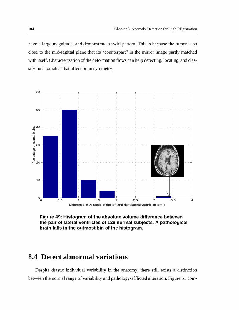
104 Chapter 8 Anomaly Detection thrOugh REgistration
havea largemagnitude,anddemonstratea swirl pattern.This is becausethe tumor is so
closeto the mid-sagittalplanethat its “counterpart”in the mirror imagepartly matched
with itself.Characterizationof thedeformationflows canhelpdetecting,locating,andclas-
sifying anomalies that affect brain symmetry.
8.4 Detect abnormal variations
Despitedrastic individual variability in the anatomy,therestill existsa distinction
betweenthenormalrangeof variability andpathology-afflictedalteration.Figure51com-
0 0.5 1 1.5 2 2.5 3 3.5 40
10
20
30
40
50
60
Per
cent
age
of n
orm
al b
rain
s
Difference in volumes of the left and right lateral ventricles (cm3)
Figure 49: Histogram of the absolute volume difference betweenthe pair of lateral ventricles of 128 normal subjects. A pathologicalbrain falls in the outmost bin of the histogram.

105
pares the label, skull, between the atlas and a brain with chronic subdural hematoma. The
Skull in the pathological brain was segmented by registering with the atlas, and thus cus-
tomizing the volumetric classification in the atlas. Note that the skull in the atlas has uni-
form thickness, with variations within a small range, whereas the thickness of skull in the
pathological brain varies significantly. This is because the pathology, hematoma, is non-
existent in the atlas. During registration, it was mistakenly matched to the neighboring
structure with similar intensity, the skull.
Bleeding TumorNormal
Figure 50: Several subjects (top) and the deformations incurred inmatching their mirror images to the original volumes (bottom overlay).Large deformations present for pathological cases.

106 Chapter 8 Anomaly Detection thrOugh REgistration
A statisticalstudyof theskull volumeovera populationof 48 normalsubjectsgivesa
histogramdistributionshownin Figure52.Thehorizontalaxisis thevolumeof theskull in
cm3, theverticalaxis is thepercentageof subjectsstudied.Note thewide rangeof varia-
tions amongnormal subjects.The estimatedskull volume in the pathologicalbrain is
106.57cm3, which falls beyondthenormaldistribution.Combinedwith theanalysisusing
symmetry, this can be used as another clue for anomaly detection.
8.5 Chapter summary
Thischapterpresentedexplorationsin usingregistrationfor pathologydetection.Com-
bining analysisof normal asymmetryand normal rangeof variationsin a population,
pathologiesthataffectbrainmorphologycanbeindicated.However,white matterlesions
suchasmultiplesclerosisdonotcausesignificantdistortionof apatient’sanatomy,which
Figure 51: Comparing the label, skull, between a normalbrain and a brain with chronic subdural hematoma.
Skull
Normal brain Pathological brain

107
makes it difficult for deformable registration to detect. Approaches combining statistical
classification and deformable registration may promise to overcome the limitations, as pro-
posed in [105].
100 200 300 400 500 600 700 800 900 1000 1100 12000
5
10
15
20
25
30
Per
cent
age
of n
orm
al b
rain
s
Skull Volume (cm3)
Figure 52: Histogram of the skull volume of 48 normal subjects. Apathological brain falls beyond the normal range of variations.

108 Chapter 8 Anomaly Detection thrOugh REgistration

109
CHAPTER 9 Conclusion
This thesis has focused on extracting and modeling the knowledge of non-pathological
anatomical variabilities between individuals, and the application of such knowledge to
achieve more accurate registration than traditional image-based correspondence. Inherent
anatomical variations are automatically extracted by deformably registering training data
with an expert-segmented 3-D image, a digital brain atlas. Statistical properties of the den-
sity and geometric variations in brain anatomy are evaluated and encoded into the atlas to
build a statistical atlas. These statistics can function as prior knowledge to guide the auto-
matic registration process. Compared to an algorithm with no knowledge guidance, regis-
tration using the statistical atlas reduces the overall error on 40 test cases by 34%.
The designed algorithm is fully automatic, efficient, and has an accuracy comparable
to human performance. When a pre-segmented image volume, referred to as an atlas, is reg-
istered to a new input image data, referred to as a subject, the anatomical segmentation in
the atlas can be customized for the subject. This reduces the months-long manual segmen-
tation process to minutes, thus enables applications such as quantitative study of anatomical
differences between populations on statistically significant data archives, and objective
110 Chapter 9 Conclusion
cross-validationof differentresearchers’discoveries.In addition,characterizationof non-
pathologicalvariationsfacilitatesdetectionof abnormalvariationsindicativeof possible
pathologies.
9.1 Highlights of Contributions
Registration Algorithm
(i) 3-D hierarchical deformable registration algorithm (Chapter2): an automatic, effi-cient, and reasonably accurate algorithm that can be employed to extract anatomicalvariabilities between individuals.
• 3-D grid-based deformable registration (Section2.2).
• Hierarchical intensity equalization,specifically the structure-basedintensitytransformation (Section2.3).
(ii) Registration using the statistical atlas to achieve higher accuracy (Chapter4 andChapter5).
• Probabilistic matching under Bayesian formulation (Chapter4).
• Weighted-window matching to incorporate neighborhood context (Chapter5).
(iii) Efficient implementation techniques, enabling fast deformable registration of 3-Dimages (Chapter6). To register 3-D images of 256x256x124 voxels on an SGI work-station with four 194 MHz processors, the 3-D hierarchical deformable registrationalgorithmtakes18minutes,registrationusingvoxel-basedstatisticstakes35minutes,and registration with neighborhood context takes 57 minutes.
• Random initialization (Section6.3).
• Adaptive multi-resolution processing (Section6.2).
Extraction of Anatomical Variabilities
(i) Automatic extraction and characterization of non-pathological anatomical variationsbetween individuals (Chapter3).
• Knowledgeextractionfrom a considerablepopulationof 105normalbrainMRIvolumes.This is a largerpopulationthanwhatis employedin mostrelatedwork.
(ii) A 3-D statistical atlas (Chapter3): a global, volumetric representation of anatomicalvariabilities between individuals.

111
(iii) Bootstrap strategy to reduce imprecisions in knowledge models propagated frominaccurate automatic registration.
Quantitative Evaluation of Registration Performance
(i) Quantitativeevaluationof performanceonasizabletestsetof 40MRI volumes.Thisis considerably larger than what is used in most related work.
(ii) Developed and demonstrated the efficacy of two new performance metrics for quanti-tative evaluation of 3-D registration results (Section2.4.2, Section5.4).
(iii) Registration accuracy of 2.9% overall error compared to expert performance. This isarguably one of the most accurate deformable registration results published.Figure53 compares registration results given by each level of the 3-D hierarchicaldeformable registration, registration using voxel-based statistics, and registrationusing neighborhood context. The reduction in error ratio is significant along the hier-archical deformation (Figure53 a), and considerable while more comprehensiveknowledge model is employed (Figure53 b).
Applications
(i) Feasibility study of applications in quantitative analysis of anatomical differencesbetween populations, with results highly correlated to human operation (Chapter7).
(ii) Experimentsonusingknowledgeof non-pathologicalvariabilitiesto detectabnormalvariations that are indicative of pathologies (Chapter8).
(iii) Mirror-registration for asymmetry detection (Chapter8).
9.2 Future Directions
This thesishasinvestigatedtheproblemsof extractingandmodelinganatomicalvari-
abilitiesbetweenindividuals,theapplicationof suchknowledgeto achieveaccurateregis-
tration,andtheuseof registrationto quantitativelystudyanatomicaldifferencesbetween
populations.Thecurrentresearchis anearlyinvestigationin thevastandlargelyunknown
field of computational anatomy, much remains to be explored and refined.
9.2.1 Methodology
One important issueis to refine the statisticalatlasby building population-specific
atlases.To producepopulationspecificrepresentationsof anatomy,datafrom largepopu-

112 Chapter 9 Conclusion
lationsneedto bestratifiedinto subpopulationsaccordingto age,diseasestate,genderand
otherdemographiccriteria.Brainatlasesconstructedfrom subpopulationsencodeinforma-
tion on populationvariability, andthereforecanfacilitatestudyof identifying group-spe-
cific patternsof anatomicor functionalalterations.Researchersat theLaboratoryof Neuro
Imagingin theUniversityof CaliforniaatLosAngeles,arebuildingpopulation-baseddig-
ital brain atlasesfor Alzheimer’s Diseaseand schizophrenia.Atlasesfor different age
groups will also help studying anatomical changes in development and aging.
Under the currentimplementation,the training set is mappedto the atlas’ reference
frame using an automaticregistrationalgorithm with inaccuracies;intensity differences
No Knowledge Guidance Voxel−Based Statistics Neighborhood Context 0
0.5
1
1.5
2
2.5
3
3.5
4
4.5
% o
f m
isla
be
lle
d v
oxe
ls
Global Alignment Smooth Deformation Fine−tuning Deformation Voxel−Based Statistics Neighborhood Context 0
10
20
30
40
50
60
% o
f m
isla
belled v
oxels
Figure 53: Comparison of registration performance usingthe algorithm with no knowledge guidance, using thestatistical atlas , and using neighborhood context.

113
caused by image acquisition are separated from inherent tissue density variations using
hierarchical intensity equalization, which also contains imprecisions. Errors in registration
and intensity normalization affect the accuracy of models of anatomical variabilities, and
thus the rigorousness of using such models as prior knowledge to further guide registration.
One practical approach to alleviate this problem is to build an initial statistical atlas from a
small but accurately registered training set, then bootstrap it into a model based on a con-
siderable training set. Modeling the effects of different parameter settings on an MRI
machine will help more accurately remove extrinsic intensity discrepancies (Section 2.6.1).
Another issue warrants further study is the choice of knowledge models. The current
models prove to be effective and simple, but higher-level, more compact models will be
necessary to express 3-D shape variations of individual structures. Many researchers are
exploring shape models based on modal analysis, finite element analysis, and morphomet-
rics. The preliminary investigation on using PCA (Appendix B) is also one avenue to pur-
sue.
As observed in registering more than two hundred image volumes, some structures are
easily registered, whereas some others are more difficult to be matched. Therefore, a
coarse-to-fine approach that first registers the easy structures and then use them to boot-
strap the match of the more difficult ones will be helpful. Similar idea was used in the hier-
archical intensity equalization scheme (Section 2.3). Kapur et al. employed such strategy
in MRI segmentation using a relative geometric prior (prior distribution on the geometry of
difficult structures, given the geometry of easy structures) [49].
It is noteworthy that the underlining assumption to the construction of the statistical
atlas is that an individual anatomical image can model the morphometric variations
observed in other individual images. Under this assumption, the mappings between differ-
ent images are homologous, which means they only map corresponding structures and fail
to capture the changes due to topological discrepancies. Thus a morphometric analysis only
partially describes the shape differences. While the assumption that there exists a 1-to-1
correspondence between two brains is never strictly true, such as the recently reported dif-

114 Chapter 9 Conclusion
ference in sulcal patterns between Einstain and average people, the validity of this assump-
tion depends on the spatial scale of comparison. Topology of the cortex is not consistent
for different subjects, but this is a completely different problem, complex enough to war-
rant a separate research project. Approaches proposed by researchers include extracting the
cortical surface and mapping it onto a simple parametric space with the same topology, e.g.,
a sphere.
9.2.2 Applications
Quantitative analysis of the anatomy and pathology detection are the few applications
investigated in this thesis, additional exciting areas remain to be explored.
9.2.2.1 Database retrieval
The introduction of large scale PACS (Picture Archival and Communication Systems)
has resulted in the creation of large digital image databases. A typical radiology department
generates between 100, 000 and 10, 000, 000 images per year. A filmless imaging depart-
ment such as the Baltimore VA Medical Center generates approximately 1.5 terabytes of
image data annually. This has substantially increased the complexity and number of images
presented to radiologists and other physicians. Efficient retrieval in medical databases will
benefit experts, as well as non-experts, in applications such as computer-aided diagnosis,
time evolution analysis and forecasting.
Albeit a relatively new domain, medical image database retrieval has attracted much
research attention. Korn et al. examined the problem of finding similar tumor shapes so as
to search for nearest neighbors in large collections of tumor-like shapes [55]. Berrut et al.
developed a specialized user interface which allows a radiologist to semi-automatically
index images represented by a general model [4]. Liu and Dellaert employed image classi-
fication to retrieve similar cases in a well-defined database, where the distance metric
defining a classifier functioned as the similarity metric [60]. Guimond and Subsol
approached the retrieval of volume of interest (VOI) using intensity-based deformable reg-
istration between the VOI given by a user and images in the database [37]. Morphological

115
similarity is measured using correlation. Researchers at Los Alamos National Lab have
developed CANDID algorithm to retrieve similar CT slices with lung diseases using tex-
ture analysis [50]. Quantification of registration results can also be used to compare image
data and to classify similar cases.
9.2.2.2 Data-mining
Accurate and efficient registration algorithms can also facilitate data mining that detect
correlations among shapes, diagnosis, symptoms, and demographic data. This will help
form and test hypothesis about the development and treatment of diseases, study potential
relationships between subtle neuroanatomical changes and symptom severity, prognosis,
and the capacity to respond to treatment.
9.2.2.3 Model anatomical abnormalities
Various neurological disorders affect the gross anatomical shape of different brain
structures. These changes have been studied for several decades, using both postmortem
and invasive in vivo methods. Recent advances in the contrast and resolution of MRI scan-
ners make it possible to study these shape effects in vivo and noninvasively, with the poten-
tial of better diagnosis and treatment.
To properly study pathological deformations, the non-pathological inter-patient varia-
tions, such as that modeled in the statistical atlas in this thesis, need to be normalized. The
goal is to detect and quantify distributed patterns of deviation from normal anatomy [66].
For the study of asymmetry, statistical analysis of asymmetry fields will help answer ques-
tions such as the significantly asymmetrical regions in a population, the difference in asym-
metry between populations, and the detection of abnormal asymmetry [93]. Potential
approach include using vector operators such as the norm of the vector field which charac-
terizes its magnitude, the divergence of the vector field which captures its radial aspect.
High divergence and high magnitude are characteristic of atrophies or expansions due to
lesions or tumor growths,

116 Chapter 9 Conclusion
9.2.2.4 Functional atlas
The currentatlasis a structuralatlaswith anatomicalclassifications,however,there
couldalsobeatlaseson thefunctionalorganizationof thebrain,or on theresponseof dif-
ferentbrainregionsto therapeuticproceduressuchasradiotherapy.Atlasesfrom different
modalities will facilitate integration of functional and anatomical data across individuals.
9.2.2.5 From volume to surface
Morphometricvarianceof thehumanbrain is qualitativelyobservablein surfacefea-
turesof the cortex. Even sulci and gyri that consistentlyappearin all normal subjects
exhibit pronouncedvariability in sizeandconfiguration.Sulci separatefunctionally dis-
tinct regionsof thebrain,andprovideanaturaltopographicpartitionof its anatomy.Most
of thejunctionalzonesbetweenadjacentmicroanatomicfieldsrunalongthebedsof major
or minor cortical sulci. Striking intersubjectvariations in sulcal geometryhave been
reportedin primary motor,auditorycortex[78], visual cortex[86], aswell asthe recent
compellingreporton thepartialabsenceof oneof Einstain’ssulci. Althoughthe intrinsic
variability in sulcalconfigurationacrossindividualsis well knownandmuchresearchhas
beenconductedin thequantitativestudy[99], therangesof thenormalvariationshavenot
yet beendetermined.Statisticalanalysisof sulcal geometrywill facilitate multi-subject
atlasingandneurosurgicalstudies,andhelpstudyingneuro-degenerativediseasesthathave
dramatic decrease in the fractal dimension of the cerebral cortex, such as epilepsy [16].
9.2.2.6 Beyond human brain MRI
ThisthesisemphasizesresultsonT1-weightedMRI dataof humanbrains,however,the
algorithmis applicableto otherimagingmodalities,aswell asmedicaldataof otherbody
parts.Applicationsof thestatisticalatlasincludedetection,quantification,andmappingof
local shapechangesin 3-D medical imagesin disease,and during normal or abnormal
growthanddevelopment.Fornon-medicalapplications,thealgorithmcouldpotentiallybe
usedfor non-destructivediagnosisof malfunctioningmechanicalobjectssuchasengines,
and quality inspection of manufactured objects to detect interior defects.

117
Although the current algorithm is developed for volumetric data, the general approach
is suitable for a whole cadre of shape categorization and classification problems in which
knowledge of shape variation can be gleaned over a particular object class. For instance,
the formulation could have fruitful application in tracking and recognition of gesture, facial
expression, and gait. Furthermore, such models can provide a parameterized estimate of
principal deformations due to a specific process: manipulation, locomotion, growth, man-
ufacture, disease, wind, heat, etc.

118 Chapter 9 Conclusion

119
APPENDIX A Levenberg-MaquardtAlgorithm
Levenberg-Marquardt algorithm is a non-linear optimization algorithm based on gradi-
ent descent. Suppose a vector function expresses the residual difference at each
voxel, where is the vector of transformation parameters. The derivative of with
respect to shows how each component of will change given a change in the trans-
formation parameters .
Ideally, the goal would be to find the transformation parameters that make equal
to the zero vector:
R p( )
p R p( )
p R p( )
∆p
∆R p( ) ∂R∂p---------∆p= (19)
R p( )
R pnew( ) R pold( ) ∆R p( )+ 0= = (20)

120
Becauseof the existenceof noiseandthe innatediscrepanciesin different volumes,
cannot bereducedto thezerovectorin practice.Levenberg-Marquardtalgorithm
attemptsto minimize by adjustingthetransformationparametervector . From(19)
and (20) we have
Foragiven , therearefar morevoxelsthanthenumberof transformationparameters,
so is notasquarematrix.To solvethisover-constrainedsystemfor , Levenberg-Mar-
quardt algorithm employs the pseudo inverse method:
If matrix (23) is not of full rank, the pseudoinversewill not exist. Levenberg-Mar-
quardt algorithm adds a stabilizing term to the diagonal elements of the matrix
In eachiterationof Levenberg-Marquardtoptimization, is computedfrom thecur-
rent and . Thesummationof and gives . The is in
turn usedto computethe new . The iterationgoeson until is smallerthana user
definedthreshold,atwhichpoint thetransformationparametersthatminimizetheresidual
difference are considered to be recovered [76].
R p( )
R p( ) p
R pold( )– ∂R∂p---------∆p= (21)
p∂R∂p--------- p
∆p ∂R∂p---------
T ∂R∂p---------
1– ∂R∂p---------
TR pold( )–( )= (22)
∂R∂p---------
T ∂R∂p--------- (23)
λ
∆p ∂R∂p---------
T ∂R∂p--------- λI+
1– ∂R∂p---------
TR pold( )–( )= (24)
∆p
R pold( ) pold ∆p pold pnew R pnew( )
∆p ∆p

121
APPENDIX B Principal ComponentAnalysis
Principal component analysis (PCA) is an elegant method for handling high dimen-
sional data. In the context of studying anatomical variations, one potential approach is
using PCA to extract eigen-variations of a population. Major modes of variations may be
captured by principal eigen-variations, as well as probability distributions of the respective
coefficients for reconstructing data of the population.
Of course, it is questionable whether a small number of principal eigen-variations will
be sufficient in representing the immensely intricate anatomical variations of human brain,
and the high dimensionality of the data further complicates the problem. This thesis con-
ducts preliminary study on using PCA to improve registration performance, as well as
using PCA for classification.

122
1. Registration
Theregistrationproblemis still formulatedasfinding thedeformationthatmaximizes
the posterior probability:
is definedthesameasthatin Section3.3.1.,thedifferenceis in
therepresentationof . Insteadof beingthedistributionof pervoxeldefor-
mationflow, it isdefinedasthedistributionof coefficients of therespectiveeigen-defor-
mations :
Becauseeigen-deformationsareorthonormal,their respectivecoefficientsarestatisti-
cally independent. The above expression simplifies into
The numberof principal eigen-deformationsis decidedusing the plot of the sumof
eigenvalueswith respectto the numberof eigenvalues.FigureB-1 showsan example
wherethesumof eigenvaluesplateausafter20 eigenvalues.Therefore,thefirst 20 eigen-
deformationsareconsideredsufficientfor representingmajorvariationsin thepopulation.
2. Classification
It is observedthattheremayexistpopulationaldifferencesin theshapeof certainana-
tomicalstructures,e.g.manyresearchersfind theposteriorsectionof thecorpuscallosum
morebulbousin femalesubjectsthantheir malecounterparts[21]. Usingprincipaleigen-
vectorsto representeachdatacategory,anewinputcanbeclassifiedbasedonhowwell it
canbereconstructedby differentcategories.Mahalanobisdistanceis usedasthedistance
P Deformation Data⟨ | ⟩ P Data Deformation⟨ | ⟩P Deformation( )P Data( )
--------------------------------------------------------------------------------------------------------------=
P Data Deformation⟨ | ⟩
P Deformation( )
a i
e i
P Deformation( ) P a 1 … a i …, , ,( )=
P Deformation( ) P a i( )i
∏=

123
measurement.Supposethecategoryunderexaminationhasa meandeformation , anda
covariancematrix . For a particulardeformation , its Mahalanobisdistancefrom this
category is:
Using to representthe principal eigenvectorsgiven by PCA, and
to representthe correspondingcoefficients for reconstructing ,
becomes
0 5 10 15 20 25 30 35 40 45 500.6
0.8
1
1.2
1.4
1.6
1.8
2
2.2x 10
7
Number of EigenValues
Sum
of E
igen
Valu
es
Figure B-1. The sum of eigenvalues plateaus after 20 eigenvalues. Therefore,the first 20 eigenvectors are sufficient for representing major variations.
µ
Σ υ
D M υ µ–( )T Σ 1– υ µ–( )=
e 1 e 2 …e k, , k
a 1 a 2 … a k, , , υ D M
D M a i e iT
i∑
Σ 1– a j e jj
∑ =

124
Expand the above equation gives
Because are orthonormal vectors, simply becomes
where is the largesteigenvalue.Theintuition of this distancemeasureis illustrated
in FigureB-2. and are centers of the two categories, and ,
and aretheir respectiveeigenvectors.Pointp is classifiedascategoryf because
of shorter Mahalanobis distance.
Interestingdirectionsfor further investigationare conductingPCA on deformation
flows of controlpoints,initializing thedeformationby themeandeformationandsearching
for coefficientsof eacheigen-deformation,de-couplingshapeinformationfrom location
and scale, etc.
D M a i a j e iT Σ 1– e j
i j,∑=
e 1 e 2 …e k, , D M
D M
a i2
i∑
λ--------------=
λ
c m c f e f 1 e f 2
e m 1e m 2
e f 1
e f 2
e m 1e m 2
c m
c f
Figure B-2. The intuition of using Mahalanobis distance in classification.
P

125
APPENDIXC SegmentationComparison
This appendixcomparesexperts’segmentationof thecorpuscallosumin themid-sag-
ittal planeof 40 testcasesto thatfrom theautomaticregistrationalgorithm.All resultsare
displayedasbinaryimages,with thecorpuscallosumshownat intensity140,andtherest
of themid-sagittalplaneshownaszerointensitybackground.Errorratioof eachcaseis dis-
played below its respective automatic segmentation result.
Error Ratio = 0.6%
Expert Segmentation AutomaticSegmentation

126
Error Ratio = 3.03%
Error Ratio = 0.39%
Expert Segmentation Automatic Segmentation

127
Error Ratio = 4.92%
Error Ratio = 0.35%
Expert Segmentation Automatic Segmentation

128
Error Ratio = 5.0%
Error Ratio = 1.13%
Expert Segmentation Automatic Segmentation

129
Error Ratio = 1.42%
Error Ratio = 1.50%
Expert Segmentation Automatic Segmentation

130
Error Ratio = 1.04%
Error Ratio = 2.87%
Expert Segmentation Automatic Segmentation
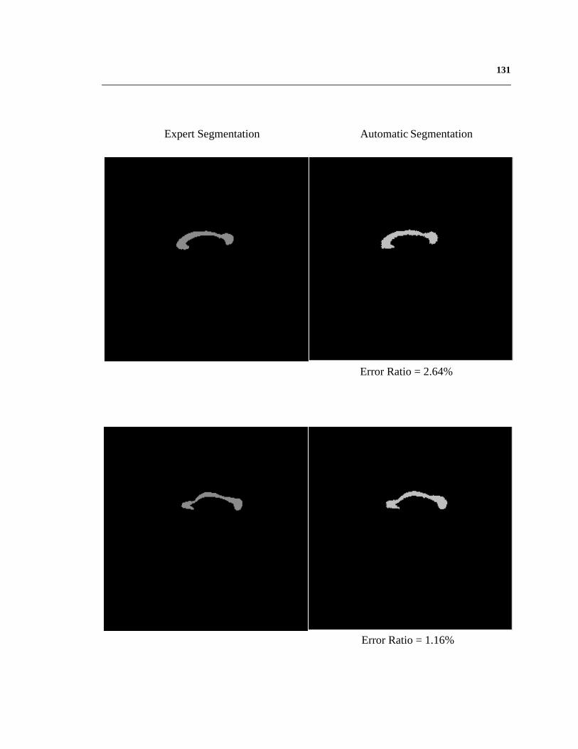
131
Error Ratio = 2.64%
Error Ratio = 1.16%
Expert Segmentation Automatic Segmentation

132
Error Ratio = 0.91%
Error Ratio = 2.35%
Expert Segmentation Automatic Segmentation

133
Error Ratio = 0.85%
Error Ratio = 2.51%
Expert Segmentation Automatic Segmentation

134
Error Ratio = 2.45%
Error Ratio = 2.05%
Expert Segmentation Automatic Segmentation

135
Error Ratio = 1.25%
Error Ratio = 7.96%
Expert Segmentation Automatic Segmentation

136
Error Ratio = 5.09%
Error Ratio = 1.02%
Expert Segmentation Automatic Segmentation
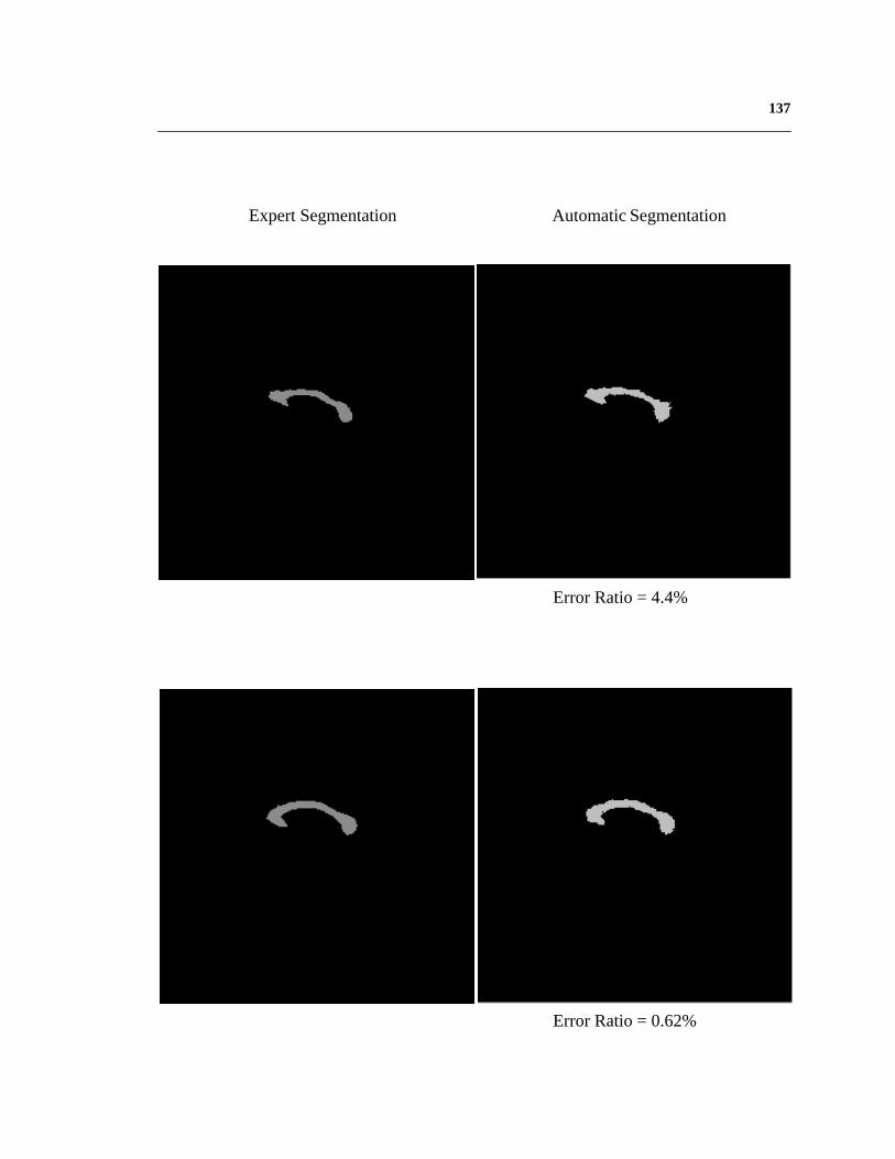
137
Error Ratio = 0.62%
Error Ratio = 4.4%
Expert Segmentation Automatic Segmentation

138
Error Ratio = 3.22%
Error Ratio = 3.87%
Expert Segmentation Automatic Segmentation

139
Error Ratio = 4.13%
Error Ratio = 3.51%
Error Ratio = 0.99%
Expert Segmentation Automatic Segmentation

140
Error Ratio = 9.78%
Error Ratio = 4.05%
Error Ratio = 3.86%
Expert Segmentation Automatic Segmentation

141
Error Ratio = 8.08%
Error Ratio = 4.15%
Error Ratio = 9.55%
Expert Segmentation Automatic Segmentation

142
Error Ratio = 5.84%
Error Ratio = 1.08%
Error Ratio = 3.78%
Expert Segmentation Automatic Segmentation

143
Error Ratio = 0.68%
Expert Segmentation Automatic Segmentation
144
Bibliography
[1] Anandan,“A computationalframework and an algorithm for the measurementofvisualmotion”, InternationalJournalof ComputerVision,vol. 2, No. 3, pp283-310,January, 1989.
[2] BajcsyandKovacic,“Multiresolution ElasticMatching”, ComputerVision, Graph-ics, and Image Processing, vol. 46, pp 1-21, 1989.
[3] Beneset al., “Normal ventriclesin youngschizophrenics”,British Journalof Psy-chiatry, vol. 141, pp. 90-93, 1982.
[4] Berrut et al., “Modeling and indexing medicalimages:the RIME approach”,Pro-ceedings of Hypertext-Information Retrieval-Multimedia, pp. 105-115, April, 1995.
[5] Besag,“On the statisticalanalysisof dirty pictures”,RoyalStatistics,B-48(3), pp.259-302, 1986.
[6] BlackandAnandan,“Robustdynamicmotionestimationover time”, ProceedingsofIEEE Conferenceon ComputerVision andPatternRecognition,pp. 296-302,June,1991.
[7] Bookstein,“Shapeandthe information in Medical Images:A decadeof the Mor-phometricSynthesis”,ComputerVision And ImageUnderstanding,vol. 66, No. 2,pp. 97-118, 1997.
[8] Bookstein,“Landmark methodsfor forms without landmarks:morphometricsofgroupdifferencesin outlineshape”,MedicalImageAnalysis,vol. 1, No. 3, pp.225-243.
[9] Chenet al., “Anomalydetectionthroughregistration”,PatternRecognition,vol. 32,pp 113-128, 1999.
145
[10] Chenetal., “3-D deformableregistrationof medicalimagesusingastatisticalatlas”,Proceedingsof the secondinternationalconferenceon Medical ImageComputingand Computer-Assisted Intervention, pp. 621-630, September, 1999.
[11] Christensenet al., “Volumetric transformationof brain anatomy”,IEEE Transac-tions on Medical Imaging, vol. 16, No. 6, December, 1997.
[12] Christensenet al., “Deformable templatesusing large deformationkinematics”,IEEE Transactions on Image Processing, September, 1996.
[13] Christensenet al., “Individualizing NeuroanatomicalAtlasesUsing A MassivelyParallel Computer”, IEEE Computer, pp. 32-38, January 1996.
[14] Collinsetal., “Automatic3-D model-basedneuroanatomicalsegmentation”,HumanBrain Mapping, vol. 3, pp 190-208, 1995.
[15] Collins et al., “Automatic 3D intersubjectregistration of MR volumetric data instandardizedTalairachspace”,Journalof ComputerAssistedTomography, vol. 18,No. 2, pp 192-205, 1994.
[16] Cooket al., “Analysisof corticalpatterns”,MagneticResonanceScanningandEpi-lepsy, pp. 263-274, Plenum, New York, 1994.
[17] Cootesetal., “Trainablemethodof parametricshapedescription”,ImageandVisionComputing, vol. 10, No. 5, pp. 289-294, June, 1992.
[18] Cootes,“Combining point distribution modelswith shapemodelsbasedon finiteelement analysis”, Proceedings of British Machine Vision Conference, 1994.
[19] Dann et al., “Evaluationof elasticmatchingsystemsfor anatomic(CT, MR) andfunctional(PET)cerebralimages”,Journalof ComputerAssistedTomography, vol.13, No. 4, pp 603-611, 1989.
[20] Davatzikos, “Spatial transformationand registrationof brain imagesusing elasti-cally deformablemodels”,ComputerVisionandImageProcessing,SpecialIssueonMedical Imaging, May, 1997.

146
[21] Davatzikoset al., “A computerizedapproachfor morphologicalanalysisof thecor-puscallosum”,Journalof ComputerAssistedTomography, vol. 20,pp.88-97,1996.
[22] Davidson and Hugdahl, “Brain Symmetry”, A Bradford Book, 1994.
[23] Declerk, et. al., “Automatic retrieval of anatomicalstructuresin 3-D medicalimages”, Technical Report 2485, INRIA, Sophia-Antipolis, France, 1995.
[24] DeLisi et al., “A prospective follow-up studyof brainmorphologyandcognitioninfirst-episodeschizophrenicpatients:Preliminaryfindings”, Biological Psychiatry,vol. 38, pp. 349-360, 1995.
[25] Evans et al., “Computationalapproachesto quantitative humanneuroanatomicalvariability”, Brain Mapping: the methods, New York, NY, Academic Press, 1996.
[26] Evanset al., “3D statisticalneuroanatomicalmodelsfrom 305MRI volumes”,Pro-ceedingsof IEEE NuclearScienceSymposiumandMedical ImagingConference,pp 1813-1817, 1993.
[27] Evanset al., “An MRI-basedstereotacticatlasfrom 250 young normal subjects”,Society of Neuroscience Abstracts, vol. 18, pp 408, 1992.
[28] Evanset al., “Warpingof Computerized3D Atlas to Match Brain ImageVolumesfor Quantitative Neuroanatomicaland FunctionalAnalysis. Proceedingsof SPIEMedical Imaging, vol. 1445, pp. 236-246, 1991.
[29] Evanset al., “MRI-PET correlationin threedimensionsusinga volume-of-interest(VOI) atlas”, Journalof CerebralBlood Flow andMetabolism,vol. 11, A69-A78,1991.
[30] FeldmarandAyache,“Locally affine registrationof free-formsurfaces”,Proceed-ingsof IEEEConferenceonComputerVisionandPatternRecognition,pp496-501,1994.
[31] GeeandLe Briquer, “An empiricalmodelof brainshape”,Maximum Entropy andBayesian Methods, August 4-8, 1997.
147
[32] Geeet al., “BayesianApproachto theBrain ImageMatchingProblem”,SPIEMed-ical Imaging, 1995.
[33] Geeet al., “Elastically Deforming3D Atlas to Match AnatomicalBrain Images”,Journal of Computer Assisted Tomography, vol. 17, No. 2, pp 225-236, 1993.
[34] Geiger and Girosi, “Parallel and deterministicalgorithms from MRFs: surfacereconstruction”,IEEE Transactionson PatternAnalysisandMachineIntelligence,vol. 13, No. 5, pp. 401-412, May, 1991.
[35] Gemanand Geman,“Stochasticrelaxation,Gibbs distributions,and the Bayesianrestorationof images”,IEEE Transactionson PatternAnalysisandMachineIntelli-gence, vol. 6, No. 6, pp. 721-741, November, 1994.
[36] GleicherandWitkin, “Through-the-lenscameracontrol”, ComputerGraphics,vol.26, No. 2, pp 331-340, July, 1992.
[37] GuimondandSubsol,“AutomaticMRI databaseexplorationandapplication”,Pat-tern Recognition and Artificial Intelligence, vol. 11, No. 8, December, 1997.
[38] Guimondet. al., “AutomaticComputationof AverageBrain Models”, Proceedingsof theFirst InternationalConferenceon Medical ImageComputingandComputer-Assisted Intervention, pp. 631-640, 1998.
[39] Haller et al., “Three-dimensionalhippocampalMR morphometrywith high-dimen-sionaltransformationof a neuroanatomicatlas”,Radiology, No. 202,pp. 504-510,1997.
[40] Hill et al., “Model-basedinterpretationof 3D medicalimages”,Proceedingsof the4th British Machine Vision Conference, pp. 339-348, 1993.
[41] Hillman etal., “Measurementof braincompartmentvolumesin MR usingcomposi-tion calculations”,Journalof ComputerAssistedTomography, vol. 15,pp.640-646,1991.
[42] Hommer et al., “Decreasedcorpus callosum size among alcoholic women”,Archives of Neurology, vol. 53, pp. 359-363, April, 1996.
148
[43] Horn,“Closed-formsolutionof absoluteorientationusingunit quaternions”,Journalof Optical Society of America, vol. 4, No. 4, April, 1987.
[44] Horn andSchunck,“Determiningoptical flow”, Artificial Intelligence,vol. 17, pp185-203, 1981.
[45] Jacobson,“The contributions of sex and drinking history to the CT brain scanchanges in alcoholics”, Psychological Medicine, vol. 16, pp. 547-559, 1986.
[46] Joshietal., “On thegeometryandshapeof brainsub-manifolds”,InternationalJour-nalof PatternRecognitionandArtificial Intelligence,vol. 11,No. 8, pp.1317-1343,1997.
[47] Joshiet al., “Hierarchical brain mappingvia a generalizedDirichlet solution formapping brain manifolds”,
[48] Kamber et al., “Model-based3-D segmentationof multiple sclerososlesions inmagneticresonancebrainimages”,IEEETransactionsonMedicalImaging,vol. 14,No. 3, pp. 442-453, September, 1995.
[49] Kapuretal., “Enhancedspatialpriorsfor segmentationof magneticresonanceimag-ery”, Proceedingsof theFirst InternationalConferenceon Medical ImageComput-ing and Computer-Assisted Intervention, pp. 457-468, 1998.
[50] Kelly andCannon,“CANDID: Comparisonalgorithmfor navigating digital imagedatabases”,Proceedingsof 7th InternationalWorking Conferenceon ScientificandStatistical Database Management, pp. 252-258, September, 1994.
[51] Keshavan et al., “Brain structural alterations in early Schizophrenia:do theyprogress?”, Journal of Psychiatric Research, 1996.
[52] Kikinis et al., “Routinequantitative analysisof brainandcerebrospinalfluid spaceswith MR imaging”, Journalof MagneticResonanceImaging,vol. 2, pp. 619-629,1992.
[53] Kikinis etal., “A digital brainatlasfor surgicalplanning,modeldrivensegmentationandteaching”,IEEE Transactionson VisualizationandComputerGraphics,vol. 2,No. 3, 1996.

149
[54] Kischell et al., “Classificationof brain compartmentsand headinjury lesionsbyneuralnetworksappliedto MRI”, DiagnosticNeuroradiology, vol. 37,pp.535-541,1995.
[55] Korn et al., “Fastnearestneighborsearchin medicalimagedatabases”,Proceedingsof Visual Libraries and DataBases, 1996.
[56] Kroft et al., “Brain ventricularsizein femalealcoholism:anMRI study”, Alcohol-ism, vol. 8, pp. 31-34, 1991.
[57] Kyriacou and Davatzikos, “A biomedicalmodel of soft tissuedeformationwithapplicationsto non-rigid registrationof brain imageswith tumor pathology”,Pro-ceedingsof the First InternationalConferenceon Medical ImageComputingandComputer-Assisted Intervention, pp. 531-538, 1998
[58] Lirio et al., “Localizationerror in biomedicalimaging”, Computersin Biology andMedicine, vol. 22, No. 4, pp 277-286, 1992.
[59] Liu etal., “Automaticbilateralsymmetry(mid-sagittal)planeextractionfrom patho-logical 3D neuroradiologicalimages”,Proceedingsof SPIE InternationalSympo-sium on Medical Imaging, February, 1998.
[60] Liu and Dellaert, “Classification-driven medical image retrieval”, Image Under-standing Workshop, November, 1998.
[61] Loncaricet al., “3-D imageanalysisof intra-cerebralbrain hemorrhagefrom digi-tizedCT films”, ComputerMethodsandProgramsin Biomedicine,vol. 46,pp.207-216, 1995.
[62] Maeset al., “Multimodality ImageRegistrationby Maximizationof Mutual Infor-mation”, IEEE Transactions on Medical Imaging, vol. 16, No. 2, April, 1997.
[63] Maintz et al., “Evaluation of ridge seekingoperatorsfor multimodality medicalimagematching”,IEEE Transactionson PatternAnalysisandMachineIntelligence,vol. 18, No. 4, April, 1996.
[64] Mannet al., “Do womendevelopalcoholicbraindamagemorereadily thanmen?”,Alcohol Clin Exp Res., vol. 16 pp. 1052-1058, 1992.
150
[65] Mariaset al., “Visualizingcerebralasymmetry”,Visualizationin BiomedicalCom-puting, pp. 411-416, Springer, Hamburg, September, 1996.
[66] Martin et. al., “Characterizationof NeuropathologicalShapeDeformations”,IEEETransactions on Pattern Analysis and Machine Intelligence, vol. 20, No. 2, 1998.
[67] McInerney andTerzopoulos,“Deformablemodelsin medicalimageanalysis:a sur-vey”, Medical Image Analysis, vol. 1, No. 2, pp 91-108, 1996.
[68] Metropolisetal., “Equationof statecalculationsby fastcomputingmachines”,Jour-nal of Chemistry and Physics, vol. 21, No. 6, p. 1087-1092, 1953.
[69] Meyer et al., “Demonstratingthe accuracy andclinical versatility of mutual infor-mationfor automaticmultimodality imagefusionusingaffine andthin-platesplinewarpedgeometricdeformation”,MedicalImageAnalysis,vol. 1, No. 3, pp195-206,1997.
[70] Miller et al., “Magnetic resonanceimagingin monitoringthe treatmentof multiplesclerosis:concertedaction guideline”, Journalof Neurology, Neurosurgery, andPsychiatry, vol. 54, pp. 683-688, 1991.
[71] Moghaddamet al., “A Bayesiansimilarity measurefor direct image matching”,M.I.T. Media Laboratory Perceptual Computing Section Technical Report No. 393.
[72] PennecandThirion, “Validationof 3-D registrationmethodsbasedon pointsandframes”, INRIA, Technical Report, No. 2470, January, 1995.
[73] PentlandandSclaroff, “Closed-formsolutionsfor physically-basedshapemodelingandrecognition”,IEEE Transactionson PatternAnalysisandMachineIntelligence,vol. 13, No. 7, July, 1991.
[74] Pokrandt,“Fast Non-SupervisedMatching: A Probabilistic Approach”, internaltechnicalreport,Institute for Real-Time ComputerSystemsandRobotics,Univer-sity of Karlsruhe, 1996.
[75] Pokrandt,“Medical imageregistration:fastfeaturespaceevaluationwith Gaussianentropy function”, internaltechnicalreport,Institutefor Real-Time ComputerSys-tems and Robotics, University of Karlsruhe, 1996.

151
[76] Presset. al., “Numerical Recipesin C”, CambridgeUniversity Press,Cambridge,England, second edition, 1992.
[77] Quam,“Hierarchical warp stereo”,ImageUnderstandingWorkshop,pp 149-155,December, 1984.
[78] Rademacheretal., “Topographicalvariationof thehumanprimarycortices:implica-tions for neuroimaging,brainmappingandneurobiology”,CerebralCortex, vol. 3,pp. 313-329, 1993.
[79] RangarajanandDuncan,“Matchingpoint featuresusingmutualinformation”, Inter-nalTechnicalReport,Departmentof DiagnosticRadiologyandElectricalEngineer-ing, Yale University, 1998.
[80] SandorandLeahy, “Surface-basedlabellingof corticalanatomyusinga deformableatlas”, IEEE Transactions on Medical Imaging, vol. 16, No. 1, February, 1997.
[81] Schulzet al., “Ventricularenlargementin teenagepatientswith schizophreniaspec-trum disorder”,AmericanJournalof Psychiatry, vol. 140, No. 12, pp. 1592-1595,December, 1983.
[82] Sclaroff andPentland,“On modalmodelingfor medicalimages:underconstrainedshapedescriptionanddatacompression”,Proceedingsof IEEE Workshopon Bio-medical Image Analysis, pp. 70-79, Seattle, 1994.
[83] Shentonet al., “Harvardbrainatlas:a teachingandvisualizationtool”, Proceedingsof Biomedical Visualization, pp. 10-17, 1995.
[84] Simonetal., “Techniquesfor fastandaccurateintrasurgical registration”,JournalofImage Guided Surgery, vol. 1, 17-29, 1995.
[85] Sponheimet al., “Stability of ventricularsizeaftertheonsetof psychosisin Schizo-phrenia”, Psychiatry Research: Neuroimaging, vol. 40, pp. 21-29, 1991.
[86] Stensaaset al., “The topography and variability of the primary visual cortex inman”, Journal of Neurosurgery, vol. 40, pp. 747-755, 1974.

152
[87] Szekely et.al., “Segmentationof 2-D and3-D objectsfrom MRI volumedatausingconstrainedelasticdeformationsof flexible Fourier contourand surfacemodels”,Medical Image Analysis, vol. 1, No. 1, pp. 19-34.
[88] Szeliski,“Bayesianmodelingof uncertaintyin low-level vision”, TechnicalReport,Computer ScienceDepartment,Carnegie Mellon University, CMU-CS-88-169,August, 1988.
[89] Szeliski,“Matching 3-D AnatomicalSurfaceswith Non-Rigid DeformationsusingOctree-Splines”,InternationalJournalof ComputerVision, vol. 18, No. 2, pp 171-186, 1996.
[90] SzeliskiandCoughlan,“Spline-BasedImageRegistration”,Digital EquipmentCor-poration, Cambridge Research Lab, Technical Report 94/1.
[91] Thevenazet al., “A pyramid approachto subpixel registrationbasedon intensity”,IEEE Transactions on Image Processing, vol. 7, No. 1, January, 1998.
[92] Thirion, “Fastnon-rigidmatchingof 3D medicalimages”,INRIA, TechnicalReportNo. 2547, May, 1995.
[93] Thirion etal., “Statisticalanalysisof normalandabnormaldissymmetryin volumet-ric medical images”, Technical Report No. 3178, INRIA, June, 1997.
[94] ThompsonandToga,“Detection,visualizationandanimationof abnormalanatomicstructurewith a deformableprobabilisticatlasbasedon randomvectorfield trans-formations”, Medical Image Analysis, vol. 1, No. 4, pp 271-294.
[95] Thompsonet al., “High-resolutionrandommeshalgorithmsfor creatinga probabi-listic 3-D surfaceatlasof the humanbrain”, NeuroImage,vol. 3, No. 1, pp 9-34,February, 1996.
[96] Thompsonand Toga, “A surface-basedtechniquefor warping three-dimensionalimagesof the brain”, IEEE Transactionson Medical Imaging,vol. 15, No. 4, pp402-417, August, 1996.
153
[97] Thompsonet al., “Mapping structuralalterationsof the corpuscallosumduringbraindevelopmentanddegeneration”,Proceedingsof theNATO ASI on theCorpusCallosum, Kluwer Academic Press.
[98] Thompsonetal., “Trackingtumorgrowth ratesin patientswith malignantgliomas”,AnnualMeetingof theSocietyfor Neuro-Oncology, Scottsdale,Arizona,November18-21, 1999.
[99] Thompsonet al., “Three-dimensionalstatisticalanalysisof sulcalvariability in thehuman brain”, Journal of Neuroscience, vol. 16, No. 13, pp. 4261-4274, July, 1996.
[100] Ullman,
[101] vandenElsen,Pol,andViergever, “Medical ImageMatching--AReview with Clas-sification”, IEEE Engineeringin MedicineandBiology, vol. 12, No. 1, pp 26-39,1993.
[102] Vemuri et al., “An Efficient Motion Estimatorwith Applicationsto Medical ImageRegistration”, Medical Image Analysis.
[103] Viola andWells III, “Alignmentby Maximizationof Mutual Information”,Proceed-ings of the fifth International Conference on Computer Vision, pp 16-23, 1995.
[104] WangandStaib,“Elastic Model BasedNon-rigid RegistrationIncorporatingStatis-tical ShapeInformation”,Proceedingsof theFirst InternationalConferenceonMed-ical Image Computing and Computer-Assisted Intervention, pp. 1162-1173, 1998.
[105] Warfield et al., “Automatic identification of grey matter structuresfrom MRI toimprove the segmentationof white matterlesions’,Journalof ImageGuidedSur-gery, vol. 1, No. 6, pp. 326-338, 1995.
[106] Wells et al., “Adaptive segmentationof MRI data”, IEEE Transactionson MedicalImaging, 1996.
[107] Westet al., “Comparisonandevaluationof retrospective intermodalitybrain imageregistration techniques”,Journalof ComputerAssistedTomography, vol. 21, pp554-566, 1997.

154
[108] Wheelerand Ikeuchi, “Iterative estimationof rotation and translationusing thequaternions”,TechnicalReport,ComputerScienceDepartment,Carnegie MellonUniversity, CMU-CS-95-215, December, 1995.
[109] Witkin et.al., “Signalmatchingthroughscalespace”,InternationalJournalof Com-puter Vision, vol. 1, pp 133-144, 1987.
[110] Woodset al., “MRI-PET registrationwith automatedalgorithm”, Journalof Com-puter Assisted Tomography, vol. 17, No. 4, pp 536-546, 1993.
[111] Woodset al., “Rapid automatedalgorithmfor aligningandreslicingPET images”,Journal of Computer Assisted Tomography, vol. 16, No. 4, pp 620-633, 1992.
[112] Zhu andYuille, “Forms:a flexible object recognitionandmodelingsystem”,Har-vard Robotics Laboratory, No. 94-1, 1993.