This is an author-deposited version published in: http://oatao.univ-toulouse.fr/ Eprints ID: 4361

To cite this document: CHIKHAOUI Oussama, GRESSIER Jérémie, GRONDIN Gilles. Spectral Volume Method: application to Euler equations and performance appraisal. In: Fifth European Conference on Computational Fluid Dynamics - ECCOMAS CFD 2010, 14-17 Jun 2010, Lisbon, Portugal.

Any correspondence concerning this service should be sent to the repository administrator: staff-oatao@inp-toulouse.fr

SPECTRAL VOLUME METHOD: APPLICATION TO EULEREQUATIONS AND PERFORMANCE APPRAISAL

Oussama Chikhaoui, Jeremie Gressier and Gilles Grondin

Departement d’Aerodynamique, Energetique et PropulsionInstitut Superieur de l’Aeronautique et de l’Espace

address 10 av. Edouard Belin - BP 54032 - 31055 Toulouse - FRANCEe-mail: oussama.chikhaoui, jeremie.gressier, gilles.grondin@isae.fr

Key words: High-order methods, Spectral volume method, Unstructured grid, Com-pressible flows

Abstract. The compact high-order ’Spectral Volume Method’ (SVM, Wang (2002)) de-signed for conservation laws on unstructured grids is presented. Its spectral reconstructionis exposed briefly and its applications to the Euler equations are presented through severaltest cases to assess its accuracy and stability. Comparisons with usual methods such asMUSCL show the superiority of SVM. The SVM method arises as a high-order accuratescheme, geometrically flexible and computationally efficient.

1

1 INTRODUCTION

Despite the constant improvements in computational and data processing ressources,the continuously growing requirements of computational fluid dynamics remain still un-satisfied. In the last decade, the CFD community showed a growing interest in high-orderapproximations for solving these issues (WENO, Discontinuous Galerkin, . . . ). An at-tractive choice is the ’Spectral Volume Method’ (SVM) proposed and developed by Wanget al.1,2,3,4.

The SVM method achieves high-order accuracy on unstructured grids through polyno-mial reconstruction within initial grid cells (spectral volumes, SV) with a subdivision ofthe SV into polygonal control volumes (CV). The spectral splitting of the SV is designedto minimize internal reconstruction oscillations (Van den Abeele et al.5,6). Moreover,the reconstructed field is continuous over the entire SV, therefore internal faces are notRiemann problems. This property reduces the fluxes computation cost and contains thelimiters problems to the SV interfaces. The flux computation is finally achieved withGaussian quadrature directly inferred from CV states ponderation with a constant andunique set of coefficients for each SV in the whole domain.

To assess the performance of the SVM method, different test cases were computed withTyphon, an unstructured open-source code. The numerical experiments were chosen tocover a large set of flow configurations from continuous quasi-incompressible problems toshock wave propagations and mixing flows. Time integration is performed with a thirdorder TVD Runge-Kutta scheme and SVM results are compared to results provided byclassic schemes such as MUSCL.

The results are up to expectations with a significant increase in accuracy and a reduc-tion in CPU time per cycle compared to a usual second order scheme method using thesame number of control volumes.

2 Spectral Volume Method for the 2D Euler equations

We consider the two-dimensional Euler equations written in the conservative form ona domain Ω with appropriate initial and boundary conditions:

∂Q

∂t+∂E

∂x+∂F

∂y= 0 (1)

with

Q =

ρρuρve

, E =

ρu

ρu2 + pρuv

u(e+ p)

, F =

ρvρuv

ρv2 + pv(e+ p)

The domain Ω is discretized into N nonoverlapping triangular cells Si (Fig.1), called

2

spectral volumes (SV’s), i.e.,

Ω =N⋃i=1

Si

Figure 1: Examples of SV splitting into CVs for second, third and fourth order

If we fix a given approximation order k, every spectral volume Si is then partitionedinto m = k(k + 1)/2 subcells, called control volume (CV’s), i.e.

Si =m⋃j=1

Cij

If q denotes a conservative variable of Q, the average value of q over a control volume isthen defined as:

qij(t) =

∫Cijq(x, y, t)dxdy

Vij, j = 1..m, i = 1..N (2)

Let us consider known all the average values over a control volume Cij in a given spectralvolume Si, we can build a polynomial pi(x, y) which is a kth order polynomial approxi-mation to the state variable, i.e.:

pi(x, y) = q(x, y) +O(hk), (x, y) ∈ Si, i = 1..N (3)

This reconstruction can be defined by the analytical resolution of:∫Cijpi(x, y)dxdy

Vij= qij(t), j = 1..m (4)

The polynomial approximation can be expressed as:

pi(x, y) =m∑j=1

Lj(x, y)qij

3

where Lj are the shape functions, i.e. :∫CijLl(x, y)dxdy

Vij= δjl (5)

Such functions can be established analytically for a given partition of Si. The shapefunctions for the fourth order SV scheme with Wang’s partition is represented on figure2.

Figure 2: Shape functions for fourth order SV with Wang’s partition

The high order reconstruction is then used to update average variables on CV. Inte-gration of equation 1 on a control volume CV gives:

dQij

dt+

1

Vij

K∑r=1

∫Ar

(f · n)dA = 0 (6)

where K is the number of faces in Cij and Ar the rth face. The integration on each facecan be performed whith a kth order accurate Gauss quadratic formula, i.e. :

∫Ar

(f · n)dA =J∑q=1

wrqf(Q(xrq, yrq)) · nrAr +O(Arhk) (7)

J = int((k + 1)/2) is the number of quadrature points per face, wrq are the Gaussquadrature weights and (xrq, yrq) are the coordinates of Gauss points. Therefore, thefollowing semi-discrete equation is obtained:

dQij

dt+

1

Vij

K∑r=1

J∑q=1

wrqf(Q(xrq, yrq)) · nrAr = 0 (8)

Finally, the resolution is achieved using a usual time integration method.

4

2.1 Spectral volumes partitions

The subdivision of a spectral volume Si in different controle volumes Cij is an essentialstep for the SVM scheme. For example, some geometric partitions can lead to degener-ated systems and thus should be excluded. The splitting procedure must conserve theexisting symmetries in a triangle, use straight edges and consider convex control volumesCVs. Fig. 3 shows different geometric partitions of a spectral volume SV for differentdesired orders. While the second order splitting definition is unique, the higher orderpartitions introduce some geometric parameters. The third order partitions is defined bytwo parameters: α = AD

ABand β = AF

AA1. The fourth order partitions have four degrees of

freedom: α = ADAB

, β = AGAR

, γ = ORAR

and δ = ALAR

. The accuracy and stability of a givenspectral volume scheme depends on the choice of these geometric parameters (Abeele atal.5).

A B

C

D

EF

G

A B

C

G

D E

I

L

J

M

F H

K

A1

A B

C

D E F

I

P

T

J

R

U

G H

S

ON

K

LM

Q

Figure 3: Geometric splitting definitions for the second, third and fourth order partitions

Table 1 sums up the different implemented and tested partitions with their geometricparameters.

Partition Order α β δ γ

SVM2 2 - - - -SVM3W 3 1/4 1/3 - -SVM3K 3 91/1000 18/100 - -SVM3K2 3 0.1093621117 0.1730022492 - -SVM4W 4 1/15 2/15 2/15 1/15SVM4K 4 78/1000 104/1000 52/1000 351/1000SVM4K2 4 0.0326228301 0.042508082 0.0504398911 0.1562524902

Table 1: Geometric parameters for the different SVM partitions

The SVMW splittings were proposed by Wang et al. and they were designed byminimizing the Lebesgue constant over the SV. Whereas the minimization of this constantprovides a good assessment of the quality of the SVM splitting, different observations

5

show that it is not a sufficient condition for the stability of the scheme. Thus, Abeele5,6

proposed other geometric splittings noted as SVMK and SVMK2.

2.2 Spectral volume method assets

The spectral volume method uses a compact stencil which is a great advantage com-pared to other high order reconstructions. The latter methods are often based on projec-tions and gradients evaluations on a quite large region of neighboring cells, which is rapidlyprohibitive in terms of computational ressources (memory, CPU time) and can lead toaccuracy deterioration, for example with stretched unstructured cells or near boundaries.

The SVM geometric splitting is designed and optimised in a spectral way to mini-mize internal reconstruction oscillations known as Runge phenomena (Fig.4). The recon-structed field is continuous over the entire SV, therefore internal faces are not Riemannproblems, which reduces the flux computation cost and contains the problem of data lim-itation to the SVs faces. The other interesting aspect of the SVM is the fact that the

Figure 4: Runge phenomenon

splitting reconstruction is homothetic: no new metric terms need be kept in memory. Theinterpolation on Gauss points for fluxes computation is directly inferred from a weightingof CV states with constant and unique coefficients for the whole domain.

Lastly, while the usual finite-volume and finite-difference methods depend strongly onthe grid quality and density, the SVM reconstruction remains exact (at a given order) onarbitrarily shaped triangles.

3 Numerical experiments

To assess the performance of the SVM method, different test cases were computed withTyphon7, an unstructured open-source code. The numerical experiments were chosen tocover a large set of flows configurations, from continuous quasi-incompressible problems,to shock wave propagations and mixing flows. Time integration is performed with a thirdorder TVD Runge-Kutta scheme and SVM results are compared to results provided byusual schemes such as MUSCL.

6

3.1 Vortex evolution problem

The first test case is a simple steady vortex evolution governed by the equation:

∂p

∂t= ρ

vθ2

r(9)

with initial conditions set to :

p = 105 − 1.161 · 302

2· exp

(1− r2

4

)

An overview of the grids obtained after the SVM splitting procedure are presentedon figure 5. The meshes were designed to have the same total number of CVs. Thethird-order TVD Runge-Kutta scheme was used for time integration.

Figure 5: Controle volumes for the second, third and fourth order SV schemes

Figure 6: Pressure profiles at different times (t=0 in black, t=2 in green, t=10 in red): SVM2 (left),SVM3K (middle) et SVM4W (right)

Figure 6 shows pressure profiles across a line passing through the vortex center att = 0, t = 2 and t = 10 for different SVM orders. The second order simulation produces asignificant damping while the intensity in the vortex center is better conserved with thethird order. With the fourth order, the peak of pressure is well resolved and preservedeven with very long time simulations.

7

In order to assess the performance of the high-order SVM, the same test case has beenperformed on three different grids with the same number of SVs, using the usual MUSCLmethod and the fourth SVM scheme. Contours of pressure are shown on the figure 7. Wecan notice that even with the coarsest grid, composed of (10× 10× 2) SV (i.e. 2000 CVfor SVM4), the solution provided by the SVM scheme is more accurate than the MUSCLsolution on the finest mesh (12800 CV).

(a)

(b)

Figure 7: Pressure contours at t = 1s for different grids: 10 × 10 × 2 (left), 40 × 40 × 2 (middle) and80× 80× 2 (right). (a) : MUSCL (b) : SVM4.

Another interesting aspect of SVM simulations is the reduction in CPU time per cyclecompared to a classic MUSCL method using the same number of control volumes (50%for 2nd order, 32%to35% for 3rd order and 22%to25% for 4th order). The CPU savingsare due to the absence of gradient evaluation for inviscid fluxes and the continuity ofstate variables through internal faces. This latter fact reduces the limitation problemsand several cases can be computed without any limitation procedure.

8

3.2 Convected Vortex

In this test case, we consider the same vortex definition as in Eq. 9. However, thevortex is not steady in the domain center but convected with a speed of Vconv = 20 on adomain of [10×10]. The boundary conditions are set to periodic in the x and y directions.No limiters were employed for the SVM simulations. For the following comparisons, thevelocity profiles are considered along a horizontal line passing through the vortex centerat t = 1: the vortex crosses the whole domain twice from left to right.

Figure 8: Overview of numerical damping of a convected vortex using MUSCL-Minmod scheme

Simulation with the classic MUSCL method are presented on figures 8 and 9 using theminmod and the Van Albada limiters. The results show the solution sensitivity to thelimitation procedure. While the theoretical maximum transverse velocity is Vymax = 30,Vymax ∼ 10 and Vymax ∼ 15 are respectively obtained for the minmod and the Van Albadasimulations, which proves that this test case is very sensitive to numerical dissipation.

9

Figure 9: Comparison of velocity profiles from MUSCL simulations with the theoretical solution (black):Minmod limiter (red) and Van Albada limiter (green).

With the SVM schemes, the velocity profile is better preserved when the order isincreased (Fig.10) . Thus, Vymax ∼ 15, Vymax ∼ 25 and Vymax ∼ 30 are obtained for thesecond, third and fourth order respectively.

Figure 10: Comparison of velocity profiles along a line through the vortex center at t = 1 (left) andkinetic energy time evolution (right)

10

3.3 Simple Mach reflection

This case deals with a classic problem of shock reflection with a Mach number Ms = 1.7and a wedge angle of θ = 25. The numerical results were obtained on a domain of[25 × 16.5] on the x − y plane with the apex of the wedge placed at x = 4.69. Theupstream shock conditions are ambient conditions, with ρa = 1.225, pa = 1.01325 · 105

and u = 0. The Riemann solver used is HLLC. All simulations were carried with theTVD RK-3 time integration scheme and a CFL = 0.5.

Figure 11: Density contours for SVM2, SVM3 and SVM4 simulations

Different experimental and computational results describe the solution to this problem.They show three shocks meeting at the triple point, namely, the incident shock, thereflected shock and the Mach stem. From the triple point emerges a slip surface thatjoins the wedge at a sharp angle. Different authors point out that the delicate featurefor numerical simulations is the capture of this slip surface across which discontinuities indensity and velocity occur (Toro8).

Density contours provided by different SVM simulations are shown on figure 11 . The

11

initial grid is an unstructured mesh with 42208 SVs: i.e. 126624 CVs for SVM2, 253248CVs for SVM3 and 422080 CVs for SVM4. All SVM simulations for this case were carriedwith no limitation procedure.

It can be notices that the thicknesses of incident and reflected shocks are larger in theSVM2 solution, while it is well resolved for the SVM3 and SVM4. The contours aroundthe slip surface are better captured when the order increases and the SVM4 solutionclearly displays the development of instabilities near the wedge.

Figure 12: Density contours: MUSCL, 800.000 CV (left) and SVM4, 422.080 CV (right)

To prove that the capture of these features and the better resolution of the flow aredue to the increasing order, other simulations have been undertaken using the MUSCLscheme.

Figure 13: Entropy contours at slip surface: MUSCL, 800.000 CV (left) and SVM4, 422.080 CV (right)

The results obtained with the SVM4 scheme were compared to those provided by theMUSCL method on a structured cartesian finer grid (Fig.12). While the unstructured gridfor SVM4 contains 422.080 CVs, the grid used for MUSCL simulation is a structured mesh

12

with twice the number of CVs, i.e. 800.000 CVs. Yet, the shocks thicknesses obtained arelarge and no improvement of the slip surface resolution is observed when increasing thenumber of CV with MUSCL method. Figure 13 clearly shows that the SVM scheme bettercaptured the slip surface: Kelvin-Helmholtz instabilities can be noticed on the shear line.These observations suggest that the better resolution of the problem is achieved by theorder increase rather than the mesh refinement.

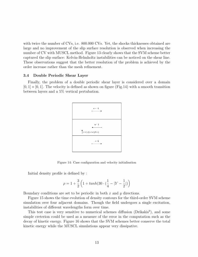
3.4 Double Periodic Shear Layer

Finally, the problem of a double periodic shear layer is considered over a domain[0, 1]× [0, 1]. The velocity is defined as shown on figure (Fig.14) with a smooth transitionbetween layers and a 5% vertical pertubation.

Figure 14: Case configuration and velocity initialisation

Initial density profile is defined by :

ρ = 1 +3

2

(1 + tanh(30 · (1

4− |Y − 1

2|))

Boundary conditions are set to be periodic in both x and y directions.Figure 15 shows the time evolution of density contours for the third-order SVM scheme

simulation over four adjacent domains. Though the field undergoes a single excitation,instabilities of different wavelengths form over time.

This test case is very sensitive to numerical schemes diffusion (Drikakis9), and somesimple creterion could be used as a measure of the error in the computation such as thedecay of kinetic energy. Figure 16 shows that the SVM schemes better conserve the totalkinetic energy while the MUSCL simulations appear very dissipative.

13

Figure 15: Density Contours

Figure 16: Double periodic shear layer: comparison of time evolution of the kinetic energy

14

4 Conclusion

In this study, analysis and applications of the Spectral Volume Method were presented.This high-order reconstruction is particularly interesting due to its compact support. Us-ing splitted control volumes with flux evaluation remains quite close to the classic Finite-Volume method which keeps the SVM implementation in existing codes relatively easy.

The results are up to expectations with a significant increase in occuracy and a re-duction in CPU time compared to a MUSCL method with the same number of elements(50% for 2nd order, 32%to35% for 3rd order and 22%to25% for 4th order). The CPU gainsare due to the absence of gradient evaluation for inviscid fluxes and the continuity ofstatus variables through internal faces. This property reduces the limitation problemsand several cases can be computed with no limitation procedure.

For all previously reported assets, the Spectral Volume Method arises as a promisinghigh-order reconstruction device for both academic and industrial studies especially forcomplex applications which require great accuracy with computational ressources savings.

Investigations in the exentension of this method to viscous flows are currently understudy. Different original choices and their implementation will be discussed in the future.

REFERENCES

[1] Z. J. Wang. Spectral (finite) volume method for conservation laws on unstruc-tured grids. basic formulation: Basic formulation. Journal of Computational Physics,178(1):210–251, May 2002.

[2] Z. J. Wang and Y. Liu. Spectral (finite) volume method for conservation laws onunstructured grids: Ii. extension to two-dimensional scalar equation. Journal ofComputational Physics, 179(2):665–697, July 2002.

[3] Z. J. Wang, L. Zhang, and Y. Liu. Spectral (finite) volume method for conservationlaws on unstructured grids iv: extension to two-dimensional systems. Journal ofComputational Physics, 194(2):716–741, March 2004.

[4] Y. Sun, Z.J. Wang, and Y. Liu. Spectral (finite) volume method for conservationlaws on unstructured grids vi: Extension to viscous flow. Journal of ComputationalPhysics, 215(1):41–58, June 2006.

[5] K. Abeele and C. Lacor. An accuracy and stability study of the 2d spectral volumemethod. Journal of Computational Physics, 226(2):1007–10026, May 2007.

15

[6] K., Abeele, M., Ghorbaniasl, M., Parsani, C., Lacor A stability analysis for thespectral volume method on tetrahedral grids Journal of Computational Physics, 228,pp. 257-265, 2009.

[7] Typhon, http://typhon.sourceforge.net/

[8] E. F. Toro. Riemann Solvers and Numerical Methods for Fluid Dynamics. Springer,1999.

[9] D. Drikakis and W. Rider. High-Resolution Methods for Incompressible and Low-Speed Flows. Springer-Verlag, 2005.

16