TM-2009-215651-PART1

Shu-cheng S. ChenGlenn Research Center, Cleveland, Ohio

Preliminary Axial Flow Turbine Design andOff-Design Performance Analysis Methodsfor Rotary Wing Aircraft Engines; I-Validation

NASA/TM—2009-215651/PART1

May 2009

NASA STI Program . . . in Profi le

Since its founding, NASA has been dedicated to the advancement of aeronautics and space science. The NASA Scientifi c and Technical Information (STI) program plays a key part in helping NASA maintain this important role.

The NASA STI Program operates under the auspices of the Agency Chief Information Offi cer. It collects, organizes, provides for archiving, and disseminates NASA’s STI. The NASA STI program provides access to the NASA Aeronautics and Space Database and its public interface, the NASA Technical Reports Server, thus providing one of the largest collections of aeronautical and space science STI in the world. Results are published in both non-NASA channels and by NASA in the NASA STI Report Series, which includes the following report types: • TECHNICAL PUBLICATION. Reports of

completed research or a major signifi cant phase of research that present the results of NASA programs and include extensive data or theoretical analysis. Includes compilations of signifi cant scientifi c and technical data and information deemed to be of continuing reference value. NASA counterpart of peer-reviewed formal professional papers but has less stringent limitations on manuscript length and extent of graphic presentations.

• TECHNICAL MEMORANDUM. Scientifi c

and technical fi ndings that are preliminary or of specialized interest, e.g., quick release reports, working papers, and bibliographies that contain minimal annotation. Does not contain extensive analysis.

• CONTRACTOR REPORT. Scientifi c and

technical fi ndings by NASA-sponsored contractors and grantees.

• CONFERENCE PUBLICATION. Collected

papers from scientifi c and technical conferences, symposia, seminars, or other meetings sponsored or cosponsored by NASA.

• SPECIAL PUBLICATION. Scientifi c,

technical, or historical information from NASA programs, projects, and missions, often concerned with subjects having substantial public interest.

• TECHNICAL TRANSLATION. English-

language translations of foreign scientifi c and technical material pertinent to NASA’s mission.

Specialized services also include creating custom thesauri, building customized databases, organizing and publishing research results.

For more information about the NASA STI program, see the following:

• Access the NASA STI program home page at http://www.sti.nasa.gov

• E-mail your question via the Internet to help@

sti.nasa.gov • Fax your question to the NASA STI Help Desk

at 301–621–0134 • Telephone the NASA STI Help Desk at 301–621–0390 • Write to:

NASA Center for AeroSpace Information (CASI) 7115 Standard Drive Hanover, MD 21076–1320

Shu-cheng S. ChenGlenn Research Center, Cleveland, Ohio

Preliminary Axial Flow Turbine Design andOff-Design Performance Analysis Methodsfor Rotary Wing Aircraft Engines; I-Validation

NASA/TM—2009-215651/PART1

May 2009

National Aeronautics andSpace Administration

Glenn Research CenterCleveland, Ohio 44135

Prepared for the65th Annual Forum and Technology Displaysponsored by the American Helicopter SocietyGrapevine, Texas, May 27–29, 2009

Available from

NASA Center for Aerospace Information7115 Standard DriveHanover, MD 21076–1320

National Technical Information Service5285 Port Royal RoadSpringfi eld, VA 22161

Available electronically at http://gltrs.grc.nasa.gov

Level of Review: This material has been technically reviewed by technical management.

This report is a formal draft or working paper, intended to solicit comments and

ideas from a technical peer group.

This report is a preprint of a paper intended for presentation at a conference. Because changes may be made before formal publication, this preprint is made available

with the understanding that it will not be cited or reproduced without the permission of the author.

NASA/TM—2009-215651/PART1 1

Preliminary Axial Flow Turbine Design and Off-Design Performance Analysis Methods for Rotary Wing

Aircraft Engines; I-Validation

Shu-cheng S. Chen

National Aeronautics and Space Administration Glenn Research Center Cleveland, Ohio 44135

Abstract For the preliminary design and the off-design performance analysis of axial flow turbines, a pair of

intermediate level-of-fidelity computer codes, TD2-2 (design; reference 1) and AXOD (off-design; reference 2), are being evaluated for use in turbine design and performance prediction of the modern high performance aircraft engines. TD2-2 employs a streamline curvature method for design, while AXOD approaches the flow analysis with an equal radius-height domain decomposition strategy. Both methods resolve only the flows in the annulus region while modeling the impact introduced by the blade rows. The mathematical formulations and derivations involved in both methods are documented in references 3, 4 (for TD2-2) and in reference 5 (for AXOD). The focus of this paper is to discuss the fundamental issues of applicability and compatibility of the two codes as a pair of companion pieces, to perform preliminary design and off-design analysis for modern aircraft engine turbines. Two validation cases for the design and the off-design prediction using TD2-2 and AXOD conducted on two existing high efficiency turbines, developed and tested in the NASA/GE Energy Efficient Engine (GE-E3) Program, the High Pressure Turbine (HPT; two stages, air cooled) and the Low Pressure Turbine (LPT; five stages, un-cooled), are provided in support of the analysis and discussion presented in this paper.

1. Introduction For the airbreathing propulsion system analysis, the NASA Glenn Research Center has previously

invested in the development of several high level design and analysis computer codes for the turbines and the compressors of the aircraft engines. Amongst these are a pair of intermediate level-of-fidelity axial flow turbine codes, TD2-2 (design; (ref. 1)) and AXOD (off-design; (ref. 2)), originally developed based on the aircraft engine technology of the 1970’s (as documented in (refs. 3 and 4) for TD2-2, and in (ref. 5) for AXOD), but subsequently modified and upgraded to suit the preliminary design and analysis purposes for the modern day axial flow, subsonic to transonic, engine turbines. Both codes are very well constructed with exceptional knowledge and expertise, and they have been extensively validated over a number (up to ten) of existing advanced axial turbines, designed and tested by either the industry or by NASA. The purpose of this paper is to describe, in principle, the methodologies and the modeling strategies currently applied in the two codes, and to discuss the issues of applicability and compatibility between the two as a pair of companion pieces, to be used in the aircraft engine turbine design and the off-design performance analysis.

The arrangement of this paper is the following: The principles of the methodology of the codes are discussed for their differences and similarities, followed by comparison of the current modeling strategies and the model closure issues of the two methods, to establish the consistency and the compatibility between the two codes. Lastly, an optimization procedure for the model closure is illustrated, and the resulting turbine performance predictions are presented and discussed through examples.

NASA/TM—2009-215651/PART1 2

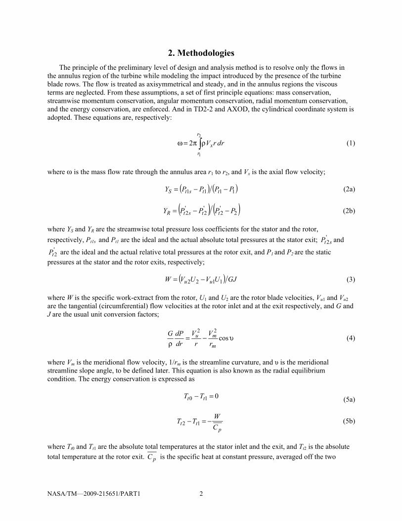
2. Methodologies The principle of the preliminary level of design and analysis method is to resolve only the flows in

the annulus region of the turbine while modeling the impact introduced by the presence of the turbine blade rows. The flow is treated as axisymmetrical and steady, and in the annulus regions the viscous terms are neglected. From these assumptions, a set of first principle equations: mass conservation, streamwise momentum conservation, angular momentum conservation, radial momentum conservation, and the energy conservation, are enforced. And in TD2-2 and AXOD, the cylindrical coordinate system is adopted. These equations are, respectively:

rdrVr

rx∫ρπ=ω

2

1

2 (1)

where ω is the mass flow rate through the annulus area r1 to r2, and Vx is the axial flow velocity; ( ) ( )1111 PPPPY ttstS −−= (2a) ( ) ( )2

'2

'2

'2 PPPPY ttstR −−= (2b)

where YS and YR are the streamwise total pressure loss coefficients for the stator and the rotor, respectively, Pt1s and Pt1 are the ideal and the actual absolute total pressures at the stator exit; '

2stP and '2tP are the ideal and the actual relative total pressures at the rotor exit, and P1 and P2 are the static

pressures at the stator and the rotor exits, respectively; ( ) GJUVUVW uu 1122 −= (3) where W is the specific work-extract from the rotor, U1 and U2 are the rotor blade velocities, Vu1 and Vu2 are the tangential (circumferential) flow velocities at the rotor inlet and at the exit respectively, and G and J are the usual unit conversion factors;

υ−=ρ

cos22

m

murV

rV

drdPG (4)

where Vm is the meridional flow velocity, 1/rm is the streamline curvature, and υ is the meridional streamline slope angle, to be defined later. This equation is also known as the radial equilibrium condition. The energy conservation is expressed as

010 =− tt TT (5a)

p

tt CWTT −=− 12 (5b)

where Tt0 and Tt1 are the absolute total temperatures at the stator inlet and the exit, and Tt2 is the absolute total temperature at the rotor exit. pC is the specific heat at constant pressure, averaged off the two

NASA/TM—2009-215651/PART1 3

stations. Lastly, a set of supplementary velocity component equations are listed to complete the system. They are:

22

rxm VVV += (6a)

22

um VVV += (6b)

( )xu VV1tan −=β (6c) ( )xr VV1tan−=υ (6d) where V is the absolute total velocity, Vr is the radial component of the flow velocity, β is the tangential flow angle, and υ is the meridional streamline slope angle.

These equations are listed in (ref. 3), and their derivations can be found in a number of textbooks, for example (ref. 6).

TD2-2 divides the annulus flow region into a number of stream tubes, each with an equal fraction of the total mass flow rate, and solves the principal equations (equations (1) to (5)) faithfully within each stream tube as a set of linear system differential equations (from the derivatives of equations (2), (3), (4), and (5); see (ref. 4)), eventually integrating the mass flow rate (equation (1)) from r1 to r2 to match the mass flow rate in the same tube upstream. This solution procedure marches axially downstream from station to station.

AXOD subdivides the flow annulus region into a number of concentric cylindrical areas of equal radius height, and assumes all relevant aerodynamic properties and the thermodynamic properties (such as the flow velocities, the total pressures, the total temperatures, and the coefficients of specific heat, etc.) are discrete constants radially within a sector (a leading order approximation, i.e., a constant within the subdivided area, but varying discretely from area to area), representable by the values obtained at the centerline of the subdivided area (sector). This treatment simplifies the solution algorithm dramatically since only the variations among a few discrete points (from sector center to sector center) at each station need to be processed, instead of having to integrate formally the whole flow domain (with an infinite number of varying points). The flow field is solved sequentially, essentially to satisfy the same set of first principle equations as that applied in TD2-2. The deficiency, of course, is the presence of discrete approximation error in the solution obtained, which is considered as a numerical error, reducible by increasing the number of sectors employed. A more fundamental error, however, is that the mass conservation in AXOD cannot be realized from an upstream station to the downstream station within each subdivided area, but can only be enforced globally by summing up all the mass flow obtained from each sector and match that to the upstream total mass flow. Since the mass conservation is not withheld within the same area element from upstream to downstream, the momentum and the energy conservations, derived for the unit mass flow rate of a conserved mass flow, expressed by equations (2), (3), and (5), are not strictly valid, but are to be regarded as an approximation to the conservation laws with the presence of approximation (true) errors. However, as was discussed and illustrated in (ref. 5), this approximation error injected into each sector is generally small, and becomes negligible with regard to the annulus area averaged physical quantities.

NASA/TM—2009-215651/PART1 4

3. Modeling Strategies and Model Closures The governing equations (1) to (5) are not a closed set of equations unless the loss coefficients

(represented by YS and YR of equations (2a) and (2b)) are properly specified. Specifying the loss mechanism and the loss coefficients constitute the primary modeling activity of the methodology discussed. TD2-2 and AXOD have two very different models and modeling strategies.

In TD2-2, the loss mechanism is the total pressure loss across a blade row from an upstream tube to the downstream tube, exactly as that expressed by equations (2a) and (2b). The coefficients of loss, YS and YR, are modeled in close form by a composite functional given in (ref. 1) as:

ex

exinS aa

aYβ+β−β=

cos|tantan|

541

(7a)

'54

''

1cos

|tantan|

ex

exinR

aaaY

β+β−β= (7b)

5.1,0.1,057.0 541 === aaa β here is the tangential flow angle, defined in equation (6c). The subscript in stands for the inflow, the subscript ex stands for the exit flow. The superscript (’) stands for quantity in the relative frame. The model constants 541 ,, aaa are obtained via validation data-fit. The rationale for the selection of this particular function is discussed in (refs. 1 and 3), briefly, the numerator |tantan| exin β−β is a tangential

blade loading factor ( tVF xu2/ ρ , t is the blade to blade spacing) and the blade row loss is expected

proportional to this quantity; the denominator exβcos is inversely proportional to the trailing edge flow blockage, and its loss contributed to the presence of the blade row is expected to be proportional to 1/

exβcos . Although simple and compact, these functions of the loss coefficients have been applied with success over ten existing turbine designs, as was illustrated in (ref. 1), which would suggest that these functional proportionalities might have captured the leading order behavior of the blade row losses.

The loss modeling applied in AXOD is more sophisticated than that in TD2-2 which is seen to have only a single mechanism, although ultimately they are to achieve the same goal, which is to close the linear momentum variation. The loss model in AXOD consists of three separate mechanisms. Firstly, the stagnation region total pressure loss factor (YA), expressed as:

20

0

01

0

02

111

MP

PPP

YA ttS ⎟⎟

⎠

⎞⎜⎜⎝

⎛ −γ

⎥⎥⎥

⎦

⎤

⎢⎢⎢

⎣

⎡

⎟⎟⎠

⎞⎜⎜⎝

⎛−⎟

⎟⎠

⎞⎜⎜⎝

⎛=

γ−γ

γ−γ

(8a)

21

1

'12

1

'1

21

11

MP

PPPYA tt

R ′⎟⎟⎠

⎞⎜⎜⎝

⎛ −γ

⎥⎥⎥

⎦

⎤

⎢⎢⎢

⎣

⎡

⎟⎟

⎠

⎞

⎜⎜

⎝

⎛−

⎟⎟

⎠

⎞

⎜⎜

⎝

⎛=

γ−γ

γ−γ

(8b)

here, 01 represents an interim state immediately after the stator inlet state 0; 12 represents the interim state immediately after the rotor inlet state of 1. The subscript t stands for the total quantities; the superscript (’) is for the quantities in the relative frame (of rotor).

NASA/TM—2009-215651/PART1 5

Secondly, the blade row kinetic energy loss coefficient (YB), expressed as:

⎟⎟

⎠

⎞

⎜⎜

⎝

⎛ −⎟⎟⎠

⎞⎜⎜⎝

⎛ −=− id

t

idt

t

tS

TTT

TTT

YB1

11

1

111 (9a-1)

⎟⎟

⎠

⎞

⎜⎜

⎝

⎛ −⎟⎟

⎠

⎞

⎜⎜

⎝

⎛ −=− idt

idt

t

tR

TTT

TTTYB '

2

2'2

'2

2'21 (9b-1)

The superscript id stands for the ideal quantities, and they are defined as:

( ) ( ) γγ

γγ 11

1011111

−−

== PPPPTT tid

tid

t (9a-2)

( )γ−γ

−γγ

γ−γ

⎟⎟⎟⎟

⎠

⎞

⎜⎜⎜⎜

⎝

⎛

⎥⎥⎥

⎦

⎤

⎢⎢⎢

⎣

⎡

⎟⎟

⎠

⎞

⎜⎜

⎝

⎛==

1

11

2'1

'2'

122'22

'2 P

TTPPPTT

t

tt

idt

idt (9b-2)

id

tT is the ideal total temperature at the stator discharge, where the flow is assumed isentropically

expanded in the stator from the interim state of 01 to the state of 1; and idtT ' is the ideal relative total

temperature at the rotor discharge, where the flow is assumed isentropically expanded in the rotor from the interim state 12 to the state of 2. In regarding the total temperatures (absolute for the stator, relative for the rotor) at discharge, we have:

01 tt TT = (9a-3) ( ) ptt GJCUUTT 22

122

'1

'2 −+= (9b-3)

here, U1 and U2 are the blade velocities at the rotor inlet and at the rotor discharge, respectively.

These equations can be derived from the texts in (ref. 5). The third loss mechanism is a blade row trailing edge blockage (flow area) loss factor (YC), expressed

simply as:

( )Sx YCAV −∗∗ρ=ω 1 (10a) ( )Rx YCAV −∗∗ρ=ω 1' (10b) where )( 2

122 rrA −π= is the sector area of the annulus at discharge.

As stated, AXOD solves the system equations sequentially, the procedure is this:

NASA/TM—2009-215651/PART1 6

(1) The interim state (01 for the stator, and 12 for the rotor) total pressure is calculated using equation (8), and the discharge total temperature, 1tT (or '

2tT ), is obtained through equation (9-3). From

these, the idtP1 (or the id

tP '2 ) is calculated using equation (9-2).

(2) A starting value for 11 PPidt (or for 2

'2 PP id

t ) is guessed (actually, that means P1 is guessed) from the mass flow function as:

( )1

1

1

1

1111

−

⎟⎟

⎠

⎞

⎜⎜

⎝

⎛∗∗γ=∗ω

PP

TT

RGMAPT

idt

idtidid

tt (11)

where,

( )1

1212

11T

TMid

tid =−γ+ (12)

(3) Equation (9) (i.e., (9a), (9b), and (9c) together) is solved to obtain the static temperature T1 (or T2)

at discharge. (4) With the static and the total temperatures known, the flow velocity components (Vx, Vu, Vr) are

calculated. And with the static pressure, temperature, and the velocities known, the sector mass flow rate ω is calculated using equation (10).

(5) The process now moves to the next sector and the steps (1), (3), and (5) are repeated, but with the static pressure at each successive sector now calculated from the radial equilibrium condition instead of from the mass flow function (of step (2)).

(6) The mass flow rate of each sector are summed, and compared to the upstream total mass flow rate for satisfying the continuity condition.

When continuity is not satisfied the iterative process starts, by successively adjusting the guessed

11 PPidt (or the 2

'2 PP id

t ) incrementally between an upper bound and a lower bound, where the upper

bound started from the value of the critical PPidt and the lower bound started with the value of one, but

successively replaced by the previously guessed ( PPidt )’s. From this, an updated PPid

t (and thus the static pressure P) is obtained. The process now goes back to step (3) above, until the mass flow rate satisfies the continuity condition from upstream.

Note that in AXOD the ( TT idt )’s are not actually being used, only the ( id

tP )’s and the ( PPidt )’s

are calculated and recorded (saved into arrays). All the ( TT idt )’s in the formula given here are to be

converted into functions of the ( PPidt )’s according to equation (9-2) when in use. And note also, that

the ( idtP )’s are the ideal total pressures at discharge, not to be confused with the actual discharge total

pressures, the ( tP )’s.

3.1 Model Closure for AXOD

Again, the solution-seeking procedure cannot commence unless the loss coefficients YA, YB, YC are specified, and interestingly, in AXOD these coefficients have not been assigned. The rationale is that, as an off-design code, the closure of the model is expected to be done consistent with the design point performance obtained through a design analysis process, which is conducted by a design code such as

NASA/TM—2009-215651/PART1 7

TD2-2. And thus the closure of the model should be done by matching to the design point performance indices obtained from the design process.

In AXOD the mechanisms for this matching process are as follow:

(1) The blade row kinetic energy loss mechanism directly impacts the ideal and the actual states of the energy content at discharge (as reflected in the values of Tt and T obtained). Thus either the efficiency (such as the total efficiency or the static efficiency) or alternatively the total-to-static temperature ratio, obtained at the design point of a design process, can be matched by adjusting YB (the blade row kinetic energy loss coefficient).

(2) At a given mass flow rate, the discharge area blockage loss directly affects the discharge flow velocity obtained, and thus it also affects the value of the static pressure at discharge. Thus, the total-to-static pressure ratio (or alternatively the blade-jet speed ratio) can be matched by adjusting YC (the blockage loss factor).

(3) The stagnation region total pressure loss factor (YA) affects the values of the ( )PPidt ’s, the

( )TT idt ’s, and ultimately the ω’s, thus this loss mechanism affects compositely the total pressure, the

static pressure, and the static temperature at discharge.

From the basic compressible flow thermodynamic relation of

1−γ

γ

⎟⎟⎠

⎞⎜⎜⎝

⎛=

TT

PP tt (13)

consider in a given system Tt is constrained (determined), for example, Tt does not change across the stator as indicated by equation (9a-3) and Tt’ is specified through equation (9b-3), thus knowing P and T would uniquely determine Pt. It appears that the loss mechanisms in AXOD are over-specified. However, as indicated, P and T are functions of (YB, YA) and (YC, YA) respectively, thus Pt is a function of all (YA, YB, YC). In other words, adjusting YA would simultaneously vary Pt, P, and T, while the three are constrained by equation (13). This is indicative of the nature that the matching between the two system solutions (from AXOD to, say TD2-2) cannot be done perfectly, but can only be done closely. Thus there is the need to specify an additional constraint as a measure of goodness of the match. We define this constraint to be

3222

⎥⎥⎥

⎦

⎤

⎢⎢⎢

⎣

⎡

⎟⎟

⎠

⎞

⎜⎜

⎝

⎛ −+⎟⎟

⎠

⎞

⎜⎜

⎝

⎛ −+⎟⎟

⎠

⎞

⎜⎜

⎝

⎛ −= d

d

d

d

dt

dtt

PPP

TTT

PPPRMSE Min= (14)

where the superscript d stands for the design point value obtained from the to-be-matched system. At any given YA, there is a corresponding set of (YB, YC) that produces a minimum RMSE; and only at a particular YA, can the absolute minimum of RMSE be reached. Thus three loss mechanisms are needed.

Clearly, when the Min is zero, the two solutions are perfectly consistent. But a more relaxed condition for the consistency between the two system solutions (at the design point) can be stated as when the RMSE reaches the absolute Min.

NASA/TM—2009-215651/PART1 8

In practice, of course, it is not the Pt , P, and T that are matched, but rather the total-to-total pressure ratio, the total-to-static pressure ratio, and the total efficiency (standard performance indices reported by almost all turbine codes) are matched to those of the given design point performance indices.

3.2 Similarity Laws for the Loss Mechanisms

With equation (14), and the mechanisms provided for the matching, the model in AXOD can be said to be closed. However, this matching process would have to be conducted from sector to sector, blade row to blade row, and stage to stage, which makes the process itself impractical. To alleviate this problem, a set of functional proportionalities (similarity laws) are defined for YA, YB, and YC. They are:

For the stagnation region total pressure loss factor (at the design condition), we define ( )expcos1 SSYA λ−= (15a-1) ( )expcos1 RRYA λ−= (15b-1) with |tantan| exinS α−α∝λ (15a-2) |tantan| ''

exinR α−α∝λ (15b-2) where, the λ’s are the stagnation region streamline deflection angles, and are assumed to be proportional to the flow circulation strength xVrπΓ 2/ generated by the blade row, which works out to be exactly that expressed by equation (15-2). The superscript exp in equation (15-1) is the order of power (the exponent), which is chosen empirically as 4 for the negative flow incidences and 3 for the positive flow incidences (given in (ref. 2); the flow incidences will be explained more later.) The α ’s are the inlet and the discharge blade angles.

For the blade row kinetic energy loss, YB, we define |tantan| exinSYB α−α∝ (16a) |tantan| ''

exinRYB α−α∝ (16b)

The rationale for this functional proportionality is as discussed previously in the loss modeling for TD2-2.

Lastly, for the trailing edge blockage loss factor, we define (again, with the same rationale as that stated in TD2-2): ( )exSYC α∝ cos/1 (17a) ( )'cos/1 exRYC α∝ (17b)

With these functional proportionalities, the loss factors YA, YB, and YC can be automatically determined from sector to sector, and/or from blade row to blade row, and/or from stage to stage, so long as a single set of (YA, YB, YC) values are explicitly specified on the meanline sector of the first stator.

NASA/TM—2009-215651/PART1 9

Note that the inlet blade angles inα (stator), 'inα (rotor) and the discharge blade angles exα (stator), '

exα (rotor) are used instead of the flow angles (the β ’s ). The blade angles are part of the geometric definitions of the turbine that are the required inputs to AXOD. Thus they are directly accessible, and in fact are more appropriate to use than the flow angles in representing the blade row characteristic functions. When the flows in the turbine blade rows are strictly subsonic, it is common that a preliminary design (not the off-design analysis) process would regard the blade angles ( ', αα ) to be equal to the flow

angles ( ', ββ ). Through these similarity laws, the functional dependency of the loss model of AXOD is seen

consistent with that of TD2-2. As an off-design code, AXOD is primarily executing at the off-design conditions. In which, the YA’s,

the YB’s, and the YC’s are all treated as invariants, based on the assumption that these dimensionless loss factors are predominantly geometric dependent (which is also reflected by the similarity relations applied here, that the dependency is only to the blade angles). As long as it is the same turbine operating at off-design, these loss factors should remain unchanged. There is, however, an additional stagnation region total pressure loss contributed from the inflow incidence effect at the off-design operation. This additional loss is augmented onto the YA’s directly as: ( )[ ]expcos1 S

ODS IdYA −= (18a-1)

( )[ ]expcos1 R

ODR IdYA −= (18b-1)

where, SininSSS IId λ+α−β=λ+= )( (18a-2) RininRRR IId λ+α−β=λ+= )( '' (18b-2) As noted, the inβ ’s are the inflow angles, and the inα ’s are the inlet blade angles. ( )α−β is the formal (by definition) inflow incidence angle I, however, the inflow-incidences reported by AXOD are actually the Id’s.

With that, the modeling in AXOD is formally closed.

4. Results and Discussion As illustrated in (ref. 1 and 2), TD2-2 and AXOD have been extensively validated. Amongst these are

two turbine designs of particular interest, the High Pressure Turbine (HPT; two stages, air cooled) and the Low Pressure Turbine (LPT; five stages, un-cooled), developed and tested in the NASA/GE Energy Efficiency Engine (GE-E3) Program. This HPT is the only cooled turbine studied, and the LPT contains the most number of stages (more challenging for the validation purpose.) Another obvious reason is that they are a pair of functioning turbines developed for the same aircraft engine. Both cases are documented with sufficiently detailed information in the GE reports, (refs. 7 and 8), in regarding the geometry, performance characteristics, and the experimental test data obtained on the turbine-built. The current study utilizes, to the extent possible, the established validation results documented in (ref. 1) and (ref. 2).

Two subjects of study are conducted here using the HPT and the LPT designs. First, the determination of the loss modeling coefficients (the design point performance indices matching process) of AXOD are conducted on the actual turbines (GE designs), and on the hypothetically designed turbines using the design code TD2-2 (cloned designs that closely follow the actual turbine geometries and the

NASA/TM—2009-215651/PART1 10

design point operating conditions), to establish the compatibility of the two codes as a pair of companion pieces. Secondly, the off-design performance predictions, using the matched loss coefficients from the actual GE turbine design-point performances and the matched loss coefficients from the TD2-2 turbine designs, are conducted and compared with each other, and with the reported experimental test data, to demonstrate the applicability of the two codes as a set of viable tools for the preliminary turbine design and analysis purposes for the aircraft engines.

4.1 Loss Coefficients Optimization Procedure

4.1.1 The HPT’s

The overall design point performance indices of the GE-E3–HPT (as reported in (ref. 7)) and that of the HPT-design performed by TD2-2 are tabulated in table 1. Again, the TD2-2 design is conducted by cloning closely to the actual GE design while operating under the same design point conditions, including estimating as closely as possible of the added coolant flows.

TABLE 1.—THE ACTUAL DESIGN POINT CHARACTERISTICS OF THE HPT’S Rating

efficiency Total-to-total

P.R. Total-to-static

P.R. Corrected

flow GE design 0.916 5.04 5.66 18.026 TD2-2 design 0.9404 4.896 5.423 18.026

Knowing the design point performance indices, the off-design code AXOD matches these

performance indices at the design point operating condition, by adjusting the loss coefficients YA, YB, and YC through the similarity laws expressed by equations (15), (16), and (17), until a minimum RMSE defined by equation (14) is achieved, thereby closing the loss models.

The resulting design point performance characteristics obtained by AXOD on the GE-E3-HPT and the TD2-2-HPT, using respectively the set of optimum loss coefficients obtained through the processes of matching, are tabulated in table 2 and listed herein for convenience and clarity. Table 2 is to be compared with table 1 for assessment of the goodness-of-match achieved.

TABLE 2.—THE OPTIMUM MATCHING OBTAINED ON THE HPT’S BY THE PROCESSES OF AXOD

Rating efficiency

Total-to-total P.R.

Total-to-static P.R.

Corrected flow

GE design 0.9155 5.046 5.657 18.0259 TD2-2 design 0.9398 4.889 5.435 18.0259

The actual matching processes conducted are illustrated here in three tiers: First, a stagnation region

streamline deflection angle (λ) is assigned, and a blade row efficiency (1-YB) is sequentially (with a constant increment) varied. At each (λ, 1-YB) combination, the blockage factor (1-YC) is varied sequentially (again with a suitable constant increment) to capture a Tier I minimum RMSE. This is illustrated in figure 1. Next, All Tier I minimums are collected and plotted against the sequentially varying blade row efficiency (1-YB), this process is repeated over a number of assigned stagnation streamline deflection angles to identify a series of Tier II minimum RMSE’s. This process is illustrated in figure 2. Lastly the Tier II minimums are plotted against the incrementally varying streamline deflection angles (λ’s) to identify the absolute (Tier III) optimum RMSE, as illustrated by figure 3.

NASA/TM—2009-215651/PART1 11

Figure 1.—Tier I Matching Process of the GE-E3-HPT.

Figure 2.—Tier II Matching Process of the GE-E3-HPT.

Matching Process / Parametric Optimization(GE-E3 HPT, the Actual Design)

Tier 1:At Streamline Deflection Angle (ANG) of 3.0 degrees

0

0.005

0.01

0.015

0.02

0.9955 0.9965 0.9975 0.9985 0.9995Blockage Factor (B.F.)

RM

SE

0.902

B.R.E. = 0.901

0.900

0.899

B.R.E. = 0.898

Matching Process / Parameter Optimization(GE-E3 HPT, the Actual Design)

Tier 2: Data Points are the Tier 1 Minimums

0

0.001

0.002

0.003

0.004

0.005

0.006

0.89 0.895 0.9 0.905 0.91Blade Row Efficiency (B.R.E.)

RM

SE

ANG = 4 deg.

ANG = 3 deg.ANG = 2 deg.

NASA/TM—2009-215651/PART1 12

Figure 3.—Tier III Matching Process of the GE-E3-HPT.

Figure 4.—Tier III Result of the Matching Process of the TD2-2-HPT.

The same tier-by-tier matching processes are conducted over the HPT of the TD2-2 design, but for

simplicity, only the Tier III result is given here in figure 4.

Matching Process / Parametric Optimization(GE-E3 HPT, the Actual Design)

Tier 3:Obtaining the Overall Optimum

0.0006

0.0008

0.001

0.0012

0.0014

0.0016

0.0018

0 1 2 3 4 5 6Streamline Deflection Angle (deg.)

RM

SE

B.R.E. = 0.900B.F. = 0.99746

B.R.E. = 0.899B.F. = 0.99818

B.R.E. = 0.901B. F. = 0.99664

The Optimum Conceived

B.R.E. = 0.900B.F. = 0.99751

B.R.E. = 0.899B.F. = 0.99833

Matching Process / Parametric Optimization(GE-E3 HPT, the TD2-2 Design)


0.0015

0.0016

0.0017

0.0018

0.0019

0.002

0 1 2 3 4 5 6 7Streamline Deflection Angle (deg.)

RM

SE

B.R.E. = 0.929B.F. = 0.98129B.R.E. = 0.928

B.F. = 0.98192

B.R.E. = 0.927B. F. = 0.98258

B.R.E. = 0.931B.F. = 0.97994

B.R.E. = 0.930B.F. = 0.98080

The Optimum Conceived

NASA/TM—2009-215651/PART1 13

The optimum loss parameters determined, respectively through these matching processes for the HPT’s are listed in table 3. These are the set of parameters explicitly specified on the meanline sector of the first stator.

TABLE 3.—THE OPTIMUM LOSS PARAMETERS OBTAINED BY THE PROCESSES OF MATCHING ON THE HPT’S

λ on the 1st stator, degrees

Blade row efficiency, 1-YB

Blockage factor, 1-YC

GE design 3.0 0.900 0.99746 TD2-2 design 2.0 0.928 0.98192

4.1.2 The LPT’s

The same procedure is conducted on the LPT’s. The overall design point performance indices of the GE-E3–LPT (as reported in (ref. 8)) and that obtained from the LPT-design by TD2-2 are tabulated in table 4. Again, the TD2-2 design is conducted by cloning closely to the actual GE-E3-LPT design while operating under the same design point conditions.

TABLE 4.—THE ACTUAL DESIGN POINT CHARACTERISTICS OF THE LPT’S

Total efficiency

Total-to-total P.R.


Corrected flow


The off-design code AXOD matches these performance indices at the design point operating

condition, by adjusting the loss coefficients YA, YB, and YC through the similarity laws expressed by equations (15), (16), and (17), until a minimum RMSE defined by equation (14) is achieved.

The resulting design point performance characteristics obtained by AXOD on the GE-E3-LPT and the TD2-2-LPT, using the respective set of optimum loss coefficients obtained through the processes of matching, are tabulated in table 5. This table is to be compared with table 4 for the goodness-of-match, and is given here for clarity and for the ease of comparison.

TABLE 5.—THE OPTIMUM MATCHING OBTAINED ON THE LPT’S BY THE PROCESSES OF AXOD

Total efficiency

Total-to-total P.R.


Corrected flow


The same tier-by-tier matching processes are conducted over the LPT’s. Again, these processes

determine the optimum loss coefficients and the best match of the design point performance indices. For simplicity, only the Tier III results are given here. The Tier I and the Tier II plots of the GE-E3-LPT are provided in the appendix as a reference.

NASA/TM—2009-215651/PART1 14

Figure 5.—Tier III Result of the Matching Process of the GE-E3-LPT.

Figure 6.—Tier III Result of the Matching Process of the TD2-2-LPT.

Matching Process / Parametric Optimization(GE-E3 LPT, the Actual Design)


0.0012

0.0013

0.0014

0.0015

0.0016

0.0017

0 0.5 1 1.5 2 2.5 3 3.5 4 4.5 5 5.5Streamline Deflection Angle (deg.)

RM

SEThe Optimum Conceived

B.R.E.= 0.962B.F. = 0.9882

B.R.E.= 0.963B.F. = 0.9882

B.R.E.= 0.965B.F. = 0.9873

B.R.E.= 0.967B.F. = 0.9872

Matching Process / Parametric Optimization(GE-E3 LPT, the TD2-2 Design)


0.0041

0.0042

0.0043

0.0044

0 0.5 1 1.5 2 2.5 3 3.5 4 4.5 5Streamline Deflection Angle (ANG; deg.)

RM

SE

4th order fit

The Optimum ConceivedB.R.E. = 0.961B.F. = 0.9849

B.R.E. = 0.961B.F. = 0.9863

B.R.E. = 0.963B.F. = 0.9852

Transitioningto

Non-physical Solution

NASA/TM—2009-215651/PART1 15

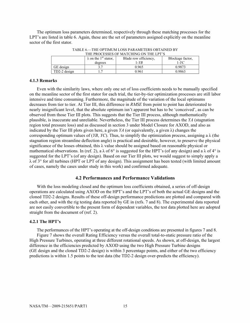
The optimum loss parameters determined, respectively through these matching processes for the LPT’s are listed in table 6. Again, these are the set of parameters assigned explicitly on the meanline sector of the first stator.

TABLE 6.—THE OPTIMUM LOSS PARAMETERS OBTAINED BY THE PROCESSES OF MATCHING ON THE LPT’S

λ on the 1st stator, degrees

Blade row efficiency, 1-YB

Blockage factor, 1-YC

GE design 3.7 0.965 0.9873 TD2-2 design 1.7 0.961 0.9863

4.1.3 Remarks

Even with the similarity laws, where only one set of loss coefficients needs to be manually specified on the meanline sector of the first stator for each trial, the tier-by-tier optimization processes are still labor intensive and time consuming. Furthermore, the magnitude of the variation of the local optimums decreases from tier to tier. At Tier III, this difference in RMSE from point to point has deteriorated to nearly insignificant level, that the absolute optimum isn’t apparent but has to be ‘conceived’, as can be observed from those Tier III plots. This suggests that the Tier III process, although mathematically plausible, is inaccurate and unreliable. Nevertheless, the Tier III process determines the YA (stagnation region total pressure loss) and as discussed in section 3 under Model Closure for AXOD, and also as indicated by the Tier III plots given here, a given YA (or equivalently, a given λ) changes the corresponding optimum values of (YB, YC). Thus, to simplify the optimization process, assigning a λ (the stagnation region streamline deflection angle) is practical and desirable, however, to preserve the physical significance of the losses obtained, this λ value should be assigned based on reasonable physical or mathematical observations. In (ref. 2), a λ of 6° is suggested for the HPT’s (of any design) and a λ of 4° is suggested for the LPT’s (of any design). Based on our Tier III plots, we would suggest to simply apply a λ of 3° for all turbines (HPT or LPT of any design). This assignment has been tested (with limited amount of cases, namely the cases under study in this work) and confirmed adequate.

4.2 Performances and Performance Validations

With the loss modeling closed and the optimum loss coefficients obtained, a series of off-design operations are calculated using AXOD on the HPT’s and the LPT’s of both the actual GE designs and the cloned TD2-2 designs. Results of these off-design performance predictions are plotted and compared with each other, and with the rig testing data reported by GE in (refs. 7 and 8). The experimental data reported are not easily convertible to the present form of dependent variables, the test data plotted here are adopted straight from the document of (ref. 2).

4.2.1 The HPT’s

The performances of the HPT’s operating at the off-design conditions are presented in figures 7 and 8. Figure 7 shows the overall Rating Efficiency versus the overall total-to-static pressure ratio of the

High Pressure Turbines, operating at three different rotational speeds. As shown, at off-design, the largest difference in the efficiencies predicted by AXOD using the two High Pressure Turbine designs (GE design and the cloned TD2-2 design) is within 3 percentage points, and either of the two efficiency predictions is within 1.5 points to the test data (the TD2-2 design over-predicts the efficiency).

NASA/TM—2009-215651/PART1 16

Figure 8 shows the corrected mass flow rate versus the total-to-static pressure ratio. Note that the test data on flow rate plotted here has been scaled by a factor of (18.19/18.026), where 18.026 is the designed mass flow rate by the computer codes, and 18.19 is the reported rig test data of the mass flow rate at the design point condition. It would be fair to scale the test data accordingly so that the code prediction and the test result are consistent to each other at the design point. In figure 8, the largest difference between the predicted mass flow rates of the two turbine designs is in the negligible difference of 0.15 percent, and the largest difference between the code predictions and the test data is within 0.6 percent.

Figure 7.—Efficiency versus Pressure Ratio of the High Pressure Turbines at Various Rotational Speeds.

Figure 8.—Mass Flow Rate versus Pressure Ratio of the High Pressure Turbines at Various Rotational Speeds.

GE-E3 HPT (2 stgs, air cooled) Efficiency MapLines -- Prediction with the Actual GE DesignDashes -- Prediction with the TD2-2 Design

Symbols -- Experimental Data by GE

0.76

0.78

0.8

0.82

0.84

0.86

0.88

0.9

0.92

0.94

0.96

2 3 4 5 6 7 8Total-to-Static Pressure Ratio

Rat

ing

Effic

ienc

y

101.6% Speed

76.2% Speed

59.3% Speed

GE-E3 HPT (2 stgs; air cooled) Flow MapLines -- Prediction with the Actual GE DesignDashes -- Prediction with the TD2-2 Design


17.8

17.85

17.9

17.95

18

18.05

18.1

18.15

18.2


Cor

rect

ed M

ass

Flow

59.3% Speed76.2% Speed

101.6% Speed

NASA/TM—2009-215651/PART1 17

4.2.2 The LPT’s

The performances of the LPT’s operating at the off-design conditions are presented in figures 9 and 10.

Figure 9.—Efficiency versus Pressure Ratio of the Low Pressure Turbines at Various Rotational Speeds.

Figure 10.—Mass Flow Rate versus Pressure Ratio of the Low Pressure Turbines at Various Rotational Speeds.

GE-E3 LPT (5 stgs, un-cooled) Efficiency MapLines -- Prediction with The Actual GE DesignDashes -- Prediction with The TD2-2 Design


0.86

0.87

0.88

0.89

0.9

0.91

0.92

0.93

0.94


Tota

l Effi

cien

cy

70% Speed

110% Speed

100% Speed

GE-E3 LPT (5 stgs, un-cooled) Flow MapLines -- Prediction with The Actual GE DesignDashes -- Prediction with The TD2-2 Design


30

31

32

33

34

35

36

37

38

39

40


Cor

rect

ed M

ass

Flow

70% Speed

100% Speed

110% Speed

NASA/TM—2009-215651/PART1 18

Figure 9 shows the overall total efficiency versus the overall total-to-static pressure ratio of the Low Pressure Turbines, operating at three different speeds of rotation. As seen, at off-design, the predicted efficiency with the actual GE design virtually coincides with the reported test data. The largest difference in the efficiencies predicted by AXOD between the two Low Pressure Turbine designs (GE design and the cloned TD2-2 design) is within 2.5 percentage points (TD2-2 design under-predicts the efficiency at off-design conditions).

Figure 10 shows the overall corrected mass flow rate versus the overall total-to-static pressure ratio of the Low Pressure Turbines, operating at three different speeds of rotation. The difference between the predicted mass flow rates of the two turbine designs, and their comparison to the reported test data, are virtually indistinguishable.

Keep in mind that the TD2-2 designs are cloning the actual GE designs at the design point condition. At off-design operations, the cloned design would understandably perform differently than the actual design, from the latter were the test data acquired. In all, the off-design performances of the cloned turbine designs by TD2-2 are consistent and competitive to the performances predicted by the actual turbine designs, and both are compared favorably to the experimental data reported.

5. Concluding Remarks The axial flow turbine design code (TD2-2) and the off-design performance analysis code (AXOD)

were presented, compared, analyzed, and validated. The methodologies, the modeling strategies, and the model closures are shown to be consistent between the two codes. The off-design performances of the cloned turbine designs using the design code TD2-2 have been shown consistent and competitive to the performances predicted by using the actual turbine designs, and both are shown to compare favorably to the experimental data reported. This indicates that the design and the off-design codes (TD2-2 and AXOD) are fundamentally consistent and compatible to each other, and the methodologies applied are mathematically and physically sound. The work presented in this paper shows that these two codes can serve as a pair of companion pieces, to be used in the subsonic to transonic, axial flow turbine designs and off-design performance predictions for the modern aircraft engines.

References 1. “Users Manual and Modeling Improvements for Axial Turbine Design and Performance Computer

Code TD2-2,” Glassman, A.J., University of Toledo, NASA CR 189118, March 1992. 2. “Modeling Improvements and Users Manual for Axial-Flow Turbine Off-Design Computer Code

AXOD,” Glassman, A.J., University of Toledo, NASA CR 195370, August 1994. 3. “Analysis of Geometry and Design Point Performance of Axial Flow Turbines; I-Development of the

Analysis Method and the Loss Coefficient Correlation,” Carter, A., Platt, M., and Lenberr, F., NREC, Cambridge, MA, NASA CR-1181, September 1967.

4. “Analysis of Geometry and Design-Point Performance of Axial-Flow Turbines Using Specified Meridional Velocity Gradients,” Carter, A. and Lenberr, F., NREC, Cambridge, MA, NASA CR-1456, December 1969.

5. “Analytical Procedure and Computer Program for Determining the Off-design Performance of Axial Flow Turbines,” Flagg, E. E., General Electric Company, Cincinnati, OH, NASA CR-710, February 1967.

6. Turbine Design and Application; Volume I, Glassman, A.J., Editor, Lewis Research Center, NASA SP-290, 1972.

7. “Energy Efficient Engine High Pressure Turbine Component Test Performance Report,” Timko, L.P., General Electric Company, Cincinnati, OH, NASA CR-168289, September 1990.

8. “NASA/GE Energy Efficient Engine Low Pressure Turbine Scaled Test Vehicle Performance Report,” Bridgeman, M., Cherry, D., and Pedersen, J., General Electric Company, Evendale, OH, NASA CR-168290, July 1983.

NASA/TM—2009-215651/PART1 19

Appendix The Tier I and the Tier II plots of the parametric matching processes conducted on the GE-E3-LPT

design are provided here (figs. 11 and 12). The Tier III plot of this LPT design is shown by figure 5 in the main text. One observes that the Tier II plot here exhibits a smoother variation than the Tier II plot of the GE-E3-HPT shown by figure 2.

Figure 11.—Tier I Matching Process of the GE-E3-LPT.

Figure 12.—Tier II Matching Process of the GE-E3-LPT.


Tier 1: At Streamline Deflection Angle (ANG) of 3.7 degrees

0.001

0.002

0.003

0.004

0.005

0.006

0.9835 0.9845 0.9855 0.9865 0.9875 0.9885 0.9895 0.9905 0.9915Blockage Factor (B.F.)

RM

SE

B.R.E. = 0.966

B.R.E. = 0.965B.R.E.= 0.967

B.R.E. = 0.964

B.R.E. = 0.963


Tier 2: Data Points are the Tier 1 Minimums

0.001

0.0015

0.002

0.0025

0.003

0.959 0.96 0.961 0.962 0.963 0.964 0.965 0.966 0.967 0.968Blade Row Efficiency (B.R.E.)

RM

SE

ANG = 2.2 ANG = 0.2 d

ANG = 4.2

REPORT DOCUMENTATION PAGE Form Approved OMB No. 0704-0188

The public reporting burden for this collection of information is estimated to average 1 hour per response, including the time for reviewing instructions, searching existing data sources, gathering and maintaining the data needed, and completing and reviewing the collection of information. Send comments regarding this burden estimate or any other aspect of this collection of information, including suggestions for reducing this burden, to Department of Defense, Washington Headquarters Services, Directorate for Information Operations and Reports (0704-0188), 1215 Jefferson Davis Highway, Suite 1204, Arlington, VA 22202-4302. Respondents should be aware that notwithstanding any other provision of law, no person shall be subject to any penalty for failing to comply with a collection of information if it does not display a currently valid OMB control number. PLEASE DO NOT RETURN YOUR FORM TO THE ABOVE ADDRESS. 1. REPORT DATE (DD-MM-YYYY) 01-05-2009

2. REPORT TYPE Technical Memorandum

3. DATES COVERED (From - To)

4. TITLE AND SUBTITLE Preliminary Axial Flow Turbine Design and Off-Design Performance Analysis Methods for Rotary Wing Aircraft Engine; I-Validation

5a. CONTRACT NUMBER

5b. GRANT NUMBER

5c. PROGRAM ELEMENT NUMBER

6. AUTHOR(S) Chen, Shu-cheng, S.

5d. PROJECT NUMBER

5e. TASK NUMBER

5f. WORK UNIT NUMBER WBS 877868.02.07.03.01.02.02

7. PERFORMING ORGANIZATION NAME(S) AND ADDRESS(ES) National Aeronautics and Space Administration John H. Glenn Research Center at Lewis Field Cleveland, Ohio 44135-3191

8. PERFORMING ORGANIZATION REPORT NUMBER E-16964-1

9. SPONSORING/MONITORING AGENCY NAME(S) AND ADDRESS(ES) National Aeronautics and Space Administration Washington, DC 20546-0001

10. SPONSORING/MONITORS ACRONYM(S) NASA

11. SPONSORING/MONITORING REPORT NUMBER NASA/TM-2009-215651-PART1

12. DISTRIBUTION/AVAILABILITY STATEMENT Unclassified-Unlimited Subject Category: 07 Available electronically at http://gltrs.grc.nasa.gov This publication is available from the NASA Center for AeroSpace Information, 301-621-0390

13. SUPPLEMENTARY NOTES

14. ABSTRACT For the preliminary design and the off-design performance analysis of axial flow turbines, a pair of intermediate level-of-fidelity computer codes, TD2-2 (design) and AXOD (off-design), are being evaluated for use in turbine design and performance prediction of the modern high performance aircraft engines. TD2-2 employs a streamline curvature method for design, while AXOD approaches the flow analysis with an equal radius-height domain decomposition strategy. Both methods resolve only the flows in the annulus region while modeling the impact introduced by the blade rows. The mathematical formulations and derivations involved in both methods are documented in a series of NASA technical reports. The focus of this paper is to discuss the fundamental issues of applicability and compatibility of the two codes as a pair of companion pieces, to perform preliminary design and off-design analysis for modern aircraft engine turbines. Two validation cases for the design and the off-design prediction using TD2-2 and AXOD conducted on two existing high efficiency turbines, developed and tested in the NASA/GE Energy Efficient Engine (GE-E3) Program, the High Pressure Turbine (HPT; two stages, air cooled) and the Low Pressure Turbine (LPT; five stages, un-cooled), are provided in support of the analysis and discussion presented in this paper. 15. SUBJECT TERMS Axial flow turbines; Preliminary design and off-design analysis methods; Rotary wing aircraft engines

16. SECURITY CLASSIFICATION OF: 17. LIMITATION OF ABSTRACT UU

18. NUMBER OF PAGES

25

19a. NAME OF RESPONSIBLE PERSON STI Help Desk (email:[email protected])

a. REPORT U

b. ABSTRACT U

c. THIS PAGE U

19b. TELEPHONE NUMBER (include area code) 301-621-0390

Standard Form 298 (Rev. 8-98)Prescribed by ANSI Std. Z39-18

TM-2009-215651-PART1

Documents

Transcript of TM-2009-215651-PART1