Title:

Author(@:

Submitted to:

STATISTICAL METHODS OF COMBINING INFORMATION: APPLICATIONS TO SENSOR DATA FUSION

Tom Burr

Joint Workshop ESARDA-INMM, Science and Modern Technology for Safeguards," Arona, Italy, October 28-31, 1996

Los Alarnos National Laboratory, an affirmative actionlequal opportunity ernpldyer, is operated by the University of California for the U S Department of Energy under contract W-7405-ENG-36 By acceptance of this article. the publisher recognizes that the U S Government retains a nonexclusive. royalty-free license to publish or reproduce the published form of this contnbution, or to allow others to do so. for U S Government purposes The LOS Alamos National LaboratOV requests that the publisher identify this article as work performed under the auspices of the U S Department of Energy Form No 836 R5

ST 2629 1 at91

DISCLAIMER

This report was prepared as an account of work sponsored by an agency of the United States Government. Neither the United States Government nor any agency thereof, nor any of their employees, makes any warranty, express or implied, or assumes any legal liability or responsibility for the accuracy, completeness, or use- fulness of any information, apparatus, product, or process disclosed, or represents that its use would not infringe privately owned rights. Reference herein to any spe- cific commercial product, process, or service by trade name, trademark, manufac- turer, or otherwise does not necessarily constitute or imply its endorsement, mom- mendirtion, or favoring by the United States Government or any agency thereof. The views and opinions of authors expressed herein do not necessarily state or reflect those of the United States Government or any agency thereof.

DECLAIMER

Portions of this document may be illegible in electronic image products. Images are produced from the best available original document.

STATISTICAL METHODS OF COMBINING INFORMATION: APPLICATIONS TO SENSOR DATA FUSION

Tom Burr Los Alamos National Laboratory, Los Alamos, New Mexico, USA

Abstract This paper reviews some statistical approaches to

combining information from multiple sources. Promis- ing “new” approaches will be described, and potential applications to combining “not-so-different’’ data sources such as sensor data will be discussed. Expe- riences with one real data set are described.

1. Introduction

Attempts to combine information from multiple sources date at least back to the invention of least squares by Legendre (1805) and Gauss (1809). The early application of least squares was to combine observations from different observatories in order to estimate the orbit of comets.

Today we have several useful formal definitions of “information.” For example, information is often related to the probability distribution of a random variable and in particular is often inversely related to the variance of that random variable. It will suffice here to think infor- mally of information as arising from either data or judg- ment. Data can usually be thought of as one or more arrays with subjects (or cases), variables, and a time andlor space index as the three or four array indices. Judgment can be subtle or obvious. Subtle judgment is made when we combine data about a single variable by reporting a summary statistic like its average over the time index. Presumably, in doing so, there was a judgment that it was meaningful to average over time. Judgment is obviously made, for example, when we write a model for the data that implies the subjects are independent or at least exchangeable.

The activity known as “combining information” can be grouped into three cases: (1) combining data and judgment within a single data set, (2) combining data and judgment from multiple data sets, and (3) combin- ing separate sources of judgment. Notice that judg- ment is present in all three cases; I know of no examples where judgment is not essential. In case three, only judgment is available. In that case some semiformal methods such as the Delphi method might be appropriate, but usually less quantitative methods are appropriate Ill. This paper is primarily concerned with cases one and two. To formally distinguish case one from case two we need to define “single data set.” For example, if drug A is tested in two clinical trials, is the data from each clinical trial a separate data set? To answer that we need to judge whether the control groups and the treatment protocol were sufficiently similar to regard the two trials as being one large trial. Experience shows that usually the two trials should be treated as separate data sets.

During the last 10 years there has been growing interest in developing formal methods to handle cases one and two. One recurring solution is some form of Bayesian analysis, particularly when the relative amounts of data and judgment are comparable. Sup- pose we want to use the observed efficacy of drug A in the two clinical trials to estimate the efficacy in some larger population. Define efficacy to be the percent p in the population that respond better to drug A than to the placebo. Expert judgment can be used within a Bayesian framework to specify a prior distribution for p , which can then be updated in various ways by the data from the two clinical trials. In most Bayesian anal- yses we must (a) solicit any prior knowledge that the Bayesian analysis requires, such as a prior probability distribution for p ; (b) use the data to update the prior to give a posterior distribution; (3) assess the sensitiv- ity of the conclusions to the choice of prior, and decide the appropriate weight between the prior knowledge and the information in the data. Bayesian analyses have always been attractive in principle but not usually in practice. The reasons that Bayesian analyses have typically been avoided include practical difficulty in choosing the prior and computational difficulty in han- dling the high dimensional integrals that often result when we try to use the posterior distribution to answer certain questions. Concerning the latter, the Gibbs sampler method represents a recent breakthrough that will move the burden of manipulating the posterior distribution from the analyst to the computer /2/. Con- cerning the former, there have been attempts to pro- duce formal procedures for eliciting prior information that have had some attention in the literature 131. More importantly, there have been many published attempts to assess the sensitivity of the conclusions to the choice of prior 141.

The field of medicine has been a major impetus in the push to develop new methods of combining infor- mation. Meta-analysis is the name most often given to combining information from multiple studies or clinical trials. Often the need for a meta-analysis arises because the data from separate trials is in conflict. For example, using data from only the first clinical trial, we might estimate p using fil = 0.7, with a standard deviation of 0.05; from the second clinical trial we might have fi2 = 0.3, with a standard deviation of 0.05. If we combined the two estimates, we might find j+, = 0.5, with a standard deviation of 0.15. On the surface it seems that we know less about p after both trials than after the first trial. The reality is that the sec- ond trial told us we were wrong in the initial assign- ment of uncertainty (interpretation of standard devia- tion) and the second trial allowed us to “recalibrate” our assessment of our ignorance about p .

We know from statistical theory that no single tool is the best for all occasions, and the same is true con- cerning the combination of information. In this paper the focus is on another method of combining data and judgment from one or more data sets: classical (non- Bayesian) multivariate time series analysis following by pattern recognition. In the time series analysis, models relating the various series will be proposed and tested, and successful models will sometimes combine data across variables. For example, we might define the sum of two time series to be a new series, or we might summarize the relation between variables by specifying their average functional relation. The analyses presented in Section 2 includes both tradi- tional and modern ways to study the functional relation among multivariate time series. In each case we must decide if the data should be treated as arising from one data set or from multiple data sets. In some cases we would fit separate models for the data from sepa- rate data sets. In other cases we would fit one model to the data from all data sets, and in most cases we choose something between those extremes. For example, if we have multiple cameras and radiation detectors monitoring the same facility, we are likely to group all cameras together and group common radia- tion detectors together, and regard the data as arising from two data sets. Or, we might use data such as the anticipated random and systematic error variances for individual radiation detectors to decide how to sub- group the radiation detectors. One of the main uses for the time series analysis is to recognize sections of abnormal background. Pattern recognition tools are applied to sections that are abnormal according to the time series model. In the example presented, addi- tional data can be provided on demand (such as when the background looks abnormal) so that the pattern recognition tools are applied to higher dimensional (more variables) data than are modeled by the time series. This situation is fairly typical, in that some form of decision theory (like control limits on control charts) is used to identify abnormal sections of data, and then either expert judgment or additional data is used to judge whether the event of interest occurred.

Time series analysis and pattern recognition are both mature fields, but progress continues in both fields. In one sense, these two fields have already been combined, at least in principle, in the safeguards area of sequential ID analysis. In that case we can either specify a specific pattern for the loss scenario or specify a class of patterns such as: the true loss is positive for 10 consecutive months. The Neyman Pearson theory is useful in such a setting. The method presented in Sections 2 and 3 is most appropriate when the amount of data is large compared to the amount of judgment, and when the class or classes of abnormal data cannot easily be described using a specific departure from the normal data.

The activity described in Sections 2 and 3 ranges from traditional to modern ways to study the functional relation among multivariate time series. In some cases

we would fit separate models for the data from sepa- rate data sets. In other cases we would fit one model to the data from all data sets, and in most cases we choose something between those extremes. For example, if we have multiple cameras and radiation detectors monitoring the same facility, we are likely to group all cameras together and group common radia- tion detectors together, and regard the data as arising from two data sets. Or, we might use data such as the anticipated random and systematic error variances for individual radiation detectors to decide how to sub- group the radiation detectors.

2. Multivariate time series followed by pattern recognition

The focus here is on the following common situa- tion: we collect time series data from multiple sensors and want to deduce the status of a monitored activity during any specified time period. For example, we might be monitoring a material processing facility that could have four statuses: (1) all processes are normal and measurements of those processes are normal (within expected uncertainties), (2) all processes are normal but some measurements are abnormal, (3) one or more processes is abnormal but all meas- urements are normal, or (4) one or more processes is abnormal and at least one measurement is abnormal. We could narrow the definition of “abnormal” by speci- fying the type of true abnormality that is the event of interest, such as removal of material from a process vessel. The Neyman-Pearson theory in classical statis- tics can sometimes be useful if we can specify the departure from normality that we want to detect. How- ever, here l will not give a specific definition of “abnor- mal” but instead will attempt to use the measured data to label all true statuses as either normal or abnormal. I then further divide “abnormal” into two types: known and fairly well characterized, such as measurement instrument failure or large measurement error, and unknown or poorly characterized. I can now state the first goal as follows:

Use time series data from multiple sensors to label each section of time as either

(1) normal, (2) abnormal of known type or of unknown type,

but not containing the event(s) of interest, or (3) abnormal and containing the event(s) of

interest. To accomplish Goal 1, I propose to use historical

data in order to set decision thresholds that will be based on the analysis of data from several sensors. Sections of data that look “abnormal” based on deci- sion thresholds will be further analyzed by pattern rec- ognition to separate false alarms from true events. Informally, the proposed approach acknowledges that classical decision theory is rarely used as textbooks describe. Rather, decision theory is often used as a ‘‘filter” to select sections of data for further analysis. In some settings, that subsequent analysis can be

assisted by pattern recognition tools, as I will demon- strate. A second goal is to increase understanding of the process and the measurements of the process, for example, by archiving the unusual sections of data and recording the times of each unusual section.

2.1 Analysis of vector time series

One widely studied class of time series model is the auto-regressive, integrated moving average (ARIMA) model that we will use to illustrate our gen- eral approach. In all cases, we require that the time series be stationary. Formal definitions of stationarity of a time series can be given, but for our purposes we simply need the mean and variance to remain the same over time. Many real times series exhibit a trend, so are therefore not stationary. Fortunately, it is simple to remove trends that are approximately polynomial in time, such as a linear or quadratic increase in the aver- age value of the times series over time. The simplest way to remove a linear trend is to compute a new time series, say Y y , that is defined by Y , = X t - X , - 1. The

new series Y , would then have a constant average value. For more detail, see Ref. 5. Now suppose that the time series { X l , X 2 , .. ., xn} has been detrended by differencing or, equivalently, by fitting polynomial func- tions of time. The detrended series is said to follow an auto-regressive, moving average (ARMA) model.

We can write the general scalar A R M A ( p , q ) model as

where the a j and bj are real constants, the E, - are independently and identically distributed (iid) random variables, and t E { 1,2, ..., n> . It is common to refer to as the shock at time t - j . Usually ARIMA

models further specify that the shock, E,, follows a

Gaussian distribution with mean 0 and variance B , denoted N ( O , B ) . In addition, to ensure that the time series is stationary (constant mean, variance, and covariances) and invertible (representable as an auto- regressive or AR model), there are conditions imposed on the values of the ai and b j .

Note that X , is a linear combination of the past p values of the series (auto-regressive) and of the past q shocks (moving average). I do not intend to restrict attention to the class of linear ARMA models, but because ARMA models are a convenient and easy-to- discuss class of models, most of our discussion will use the ARMA model for an example. Reference 6 introduced approximately 10 candidate ways to model and forecast a vector-based time series. At the time Ref. 6 was written, we had no computer algorithms for

2

vector ARMA time series. All the commercial software had a gap in that it only treated vector AR time series. It is more computationally challenging to handle vector ARMA models. To date, we have heard but not con- firmed that one lesser-known statistical programming package (JMP) can handle vector ARMA time series. We have recently added the ability to treat vector ARMA models within the statistical and graphical pro- gramming language s+ by using a user-contributed library of state-space (in the sense of the Kalman Filter language) functions. Details are part of another report 171.

The theory for vector ARIMA models is well estab- lished, though some implementation challenges remain for the vector-valued ARIMA models. There are no current completely successful methods to handle nonlinear vector autoregressive, moving average models, though an ad hoc procedure /8/ has some promise. Here I restrict attention to AR models only, for which all the classical and modern regression methods become available. For completeness here I will begin the general scalar ARMA(p, q ) model.

An AR time series can be written as follows:

The error e , is usually assumed to be from some con- venient distribution such as the Gaussian, but need not be. Nearly always the distribution of the et is at least assumed to be the same for all t . We will assume that the errors have the same distribution, F , which we write as et - F Not all functions f combined with error distribution F lead to a stationary time series. We do not attempt a formal treatment of this issue, but rather accept equation (2) as a basis for trying certain model- ing approaches.

We also easily generalize equation (2) to include other time series, say Y and Z:

+ e, . (3)

Note that present values of both Y and Z are allowed, as the goal is to forecast X . In our setting, X is the gamma series, Y is the electron series, and Z is the proton series. Or, in another setting, we have only two series: gammas and a series proportional to the sum of electrons and protons.

Equation (3) can be treated exactly like an ordinary regression model for which there are many tech- niques, loosely described by the degree of assump- tions placed on the functional form for$ I will discuss 12 models in order from the most restrictive assump- tions to least restrictive assumptions made about f. First, I point out two advantages to using restrictive models such as models that assume f is linear as follows:

3

(1) Often there is not enough data to estimate compli- cated models or completely unrestricted f . In fact, the old standby, linear regression, will be with us forever for this reason and represents an extreme example of “combining information” for which data at one end of the range is assumed to have the same functional form as data at another end of the range. By the way, because we are insisting on working with stationary series, we often must restrict the time window so that the series can be considered stationary over that window, thereby reducing the effective size of the data set and essentially forcing us to use only the simplest models. More complicated models suffer from the “curse of dimensionality,” which we will explain below.

(2) For years the regression literature has been filled with informal confirmation of the “parsimony prin- ciple” which states that simplest models are pre- ferred when possible because no data follows any model exactly, and model departures can be more severe when the training data is overfit by using an overly complex model. Fortunately, we have a straightforward way to guide us toward the proper degree of model complexity: use the model to fore- cast a held-out (not used for training) testing set, and accept the model that performs best on the testing set. A complete treatment of this issue uses what is known as cross-validation to repeatedly divide the data into training and testing sets. Cross-validation is very important when the data sets are small. In our case, we simply did a one- time division into training and testing sets because the data sets were reasonably large. One of the simplest groups of models assumes

thatfis linear in the following sense:

(4)

For notational convenience we have dropped the dis- tinction between the time series .X, Y , 2 and have lumped all candidate predictors together to form p predictors. An important issue is how to choose the lag for each of the time series. We always use a “trial-and- error” approach starting with lag 1 only for the X series (the series to be predicted) and starting with lag 0 for the other series. The winning method is the one that minimizes the sum of squared errors on a held-out testing set. If the predictors are raised to powers other than 1 we would call it a polynomial regression. Four of the 12 methods are linear regression methods: one is the traditional ordinary least squares (01s) approach that minimizes the sum of squared errors to fit param- eters ao, a l , ..., a . A second method minimizes the median (Ims) of {he squared residuals attempting to reduce sensitivity to outlying observations. The third method is a robust regression (rreg) that uses a more general “M-estimation” procedure that uses iteratively re-weighted least squares. The second and third

methods both attempt to reduce sensitivity to outlying observations that are known to cause problems with ordinary least squares. The fourth method is a class of generalized linear model (glm) that allows the user to specify the error distribution, F , and thereby use parameter estimation that is designed to be optimal for that distribution. We assumed that the error variance was approximately Poisson-distributed for this method. In fact, we know of some extreme departure from Poisson variance so we had little hope for this method. In all four cases, the forecast errors could be analyzed to suggest model departure such as nonlinearity. If nonlinearity is detected, then a good procedure is to search for a suitable transform for some of the predic- tors, or to add polynomial terms in the predictors. We have not detected nonlinearity in the forecast errors for most of the data so, in fact, we suspect that the linear models will suffice here. However, we are assembling a toolkit of model-fitting methods in anticipation of other data sets for which they might be needed. In that spirit, the next group of methods make less restrictive assumptions about f . Also included in this first group is the exponential smoother that uses a weighted aver- age (exponentially decaying weights) of the most recent observations to forecast the present observa- tion. This method is equivalent to a linear (MA) model fit to the first differences of a series, in the case we consider here. The linear (MA) model fit to the first dif- ferences of a series is denoted ARIMA(O,l,l) to denote that first differences are analyzed (original data is nonstationary) and that MA with lag 1 is used. For the exponential smoother (equivalently, the ARIMA(O,l,l)) we use only prior gammas to forecast the present gamma counts. If we used the electron and proton series we would have to adapt the expo- nential smoother more than we considered appropri- ate at this time.

A second group of methods consists of general- ized additive model (GAM), multivariate adaptive regression with splines (MARS), and projection pursuit regression (PPREG). All of these methods restrict the functional form for f somewhat, but not nearly as much as the linear methods.

The GAM model assumes

(5)

Certainly, equation (5) generalizes equation (4), as the individual f j are arbitrary smooth functions. Equation (5) is called additive to emphasize that none of the p predictors “interact” so, for example, there is no term such as f12(xIx1). If such interaction terms are con- sidered necessary, then they must be put in “by hand by defining a new variable x p + = xlxl The individual fj are estimated by a “curve smoother” that can be described qualitatively with the help of Fig. 1. Figure 1 illustrates a “curve smoother” that the human eye could do quite well. Perhaps surprisingly, training

G

software to fit the smoother is nontrivial, and we dis- cuss it further in Ref. 7. Occasionally, if there is enough data following equation (2), then a multidimen- sional curve smoother is feasible. However, the idea behind the GAM model in equation (5) is that the “curse of dimensionality” can be mitigated by restrict- ing the functional form to be additive.

The MARS method is one of the most important advances in applied statistics in the last 10 years /9/. MARS is an extension of the CART (classification and regression trees, which we describe in more detail in Section 3) that addresses the weakness of CART for regression. CART’S weakness in the case of regres- sion can be explained as follows. With CART, the pre- dictor space is split into nonoverlapping regions and the predicted response is the average of the response for cases with predictors that fell into that region of the predictor space. This procedure can lead to a discon- tinuous response surface that is nearly never desir- able. The MARS methodology removed the discon- tinuity of the response surface by effectively allowing overlap between the regions. The MARS software is public domain and is available in several forms. We have experimented with a Fortran version and a ver- sion compiled for S+. Results in this report .refer to the S+ version contributed by Trevor Hastie.

The idea in PPREG is to seek M new direction vectors Z i l , Zi,, ..., Zi, and good nonlinear transforma-

tions i p l , ip,, ..., so that

because the inner product operation 6;: represents a projection of X onto the direction i i j .

The third group of models includes local regres- sion, nonparametric smoothing, and fuzzy forecaster.

Local Rearession. Figure 1 is a statistically moti- vated curve smoother that uses locally linear or quad- ratic regression.

Nonparametric Smoothing. Equation (7) is a one- dimensional curve smoother. A higher dimensional smoother is a natural extension.

Note the “hat” notation in 3 which means that the right-hand-side is an estimate of the true f . This reflects a change from all previously described models because we do not introduce an assumed restricted form for f . Therefore, we simply present an intuitive way to estimate f at the point x . That is, all data con- tributes to the estimated value via a weighted average, with weight given by the data points distance from x . A data point, say X k , that is far from x simply won’t con-

tribute much to the estimate at X , provided we choose the smoothing parameter h and the weight function w so that W ( ( X - X j ) / h ) , which is the weighting term, is small when x - Xi is large. Consider Fig. 1 again in the light of this description: for a given value X = x, the estimate for Y is mostly determined by those Y values that correspond to X values near x. This is a simple idea, but selecting the smoothing degree remains somewhat of an art despite attempts to automate the choice of bandwidth h . However, by using held-out testing sets, it is possible to do a reasonable job of

. - I. ’

** I

00 02 04 06 0 8 10

Xl

Fig. 1 - Scatterplot illustration of a one-dimensional curve smoother.

5

automating the choice of h . Experience and theory suggest that the choice of h is more critical than the choice of W . Typically simple smooth functions such as

a Gaussian-shaped function e-x are a good choice. Theoretically optimal weight functions such as the Epanechnikov kernel are sometimes suitable, but the best theoretical shape for the weight function depends on the true function f , so we are not fond of using spe- cially motivated weight functions. In fact, we nearly always use simple Gaussian weight functions and con- cern ourselves with searching for good h /lo/. The basic idea is to balance the tradeoff between bias and variance in that too little smoothing overfits the data, reducing variance but increasing bias, and the reverse occurs for too much smoothing.

2

Fuzzy Forecaster. The fuzzy forecaster has a few forms. The form used here is called a fuzzy con- troller /1 l/. In my view, the fuzzy logic approaches to modeling and forecasting time series could benefit from a more statistical approach, especially in the area of choosing the number of fuzzy regions, which is comparable to the choice of bandwidth in equation (7).

In Ref. 10, there is more detail on this last group of models, including comparison on five real and five simulated data sets. The conclusion in Ref. 10 is that the fuzzy forecaster offers no advantage over other statistically motivated curve smoothers. In fact, our view is that fuzzy logic offers no advantage over statis- tically motivated approaches in any area in which the data is numeric. Fuzzy logic was developed for situa- tions in which numeric data was not available, and it is probably best to apply it only in those unfortunate situations.

2.2. Summary of the vector AR models considered

First, we are considering vector AR models only because we have relaxed the linearity assumption. Though it may be possible (see Ref. 8 for an ad hoc “two-step” procedure that is under investigation) to treat nonlinear MA models, we will not consider that here. Once we restrict attention to AR models, we get access to a host of regression techniques that can be applied as if the data was in the usual regression set- ting: observe independent cases of data “pairs,” (X,y) , where the 2 vector is a p -component predictor vector. The only difference in our setting is that successive cases are not independent because of the serial corre- lation. However, asymptotically (as the number of cases increases) this serial correlation can be ignored for the purpose of function estimation /la.

Most real time series do not exactly follow any model, whether the model is linear or nonlinear. The challenge in such cases is to select a reasonably sim- ple model that captures the relevant behavior of the series. And many time series cannot be made station- ary (de-trended) for extremely long time periods. How- ever, many real time series change slowly enough that under their “usual behavior” some kind of model is in

effect locally. For example, a particular ARlMA model might be a reasonable model for the first 1000 obser- vations, but a different ARlMA model might be a better model for the next 1000 observations. This compli- cates the situation, because in that case, we do not care about a// changes that might occur in a time series model. As another example, a series might fol- low something like a simple ARIMA(0,l) model, also known as an MA(1) model, but with varying error vari- ance. This could be due to a probabilistic mechanism that causes the mean to affect the variance. Simply put, large numbers tend to vary more than small num- bers, so the error variance might depend on the mean of the series. Depending on the particular application, such a model change might not be of interest. For example, it is likely that the time series generated by radiation detectors counting the background will have some Poisson-type variance component. The Poisson distribution often arises in particle-counting statistics and the Poisson variance equals its mean. Therefore, we should not be surprised to see higher variability in sections of the time series where the mean is higher.

Figure 2 shows a section of two of the time series (electron and gamma counts) we considered in a recent application. We will work with data from this example throughout this paper. From this plot it appears that it will be simple to use the current elec- trons to forecast the current gammas because the electrons appear to be proportional to the gammas. In fact, forecasting the gammas using electrons with data recorded about every 8 seconds works fairly well. Figure 3 is a plot of the forecast errors in forecasting the gammas using a linear model that related current gammas to prior gammas and to current and prior electrons. We see that in the region of large variability in the gamma counts, there is also large variability in the forecast errors. This phenomena occurred for all of the models we applied. That means that all models would judge that section to be abnormal.

In Ref. 13 we report results of a suite of 12 candi- date forecast methods to a section of 878 pairs of con- current electron and gamma counts. Because this was data with 8.192 second resolution, 878 pairs represent about 2 hours of data. Here are the two ground rules: (1) Use the first 2/3 of the data (the first 586 data

pairs) to build the model. Then report the average squared forecast error over the last 1/3 of the data (the last 292 data pairs).

(2) Always test (formally with statistical tests or infor- mally with graphical tests) whether there is serial correlation in the forecast errors. If the forecast errors exhibit serial correlation, then the model is not yet acceptable because that serial correlation should be exploited in the model. Forecast error variances are reported only if the errors exhibit no serial correlation. A more complete model assess- ment could attempt to check for any serial structure in the forecast errors (not restricted to serial corre- lation, which only measures the linear structure). I have not attempted to check for nonlinear structure in the forecast errors.

0

0 200 400 MI0 800

Time (2.048 see)

01

0 200 400 600 mo Time (2.048 SCC)

Fig. 2 - Electron counts and gamma counts.

0 0 0 *

N

0 200 400 600 800

Time(8.192sec)

Fig. 3 - The forecast errors that result from a linear model relating gamma counts to electron counts.

7

The goal now is to minimize the average squared forecast error of the gammas. For most sections of this electron and gamma data set that we considered, the simple exponential smoother method is as good as any other method. However, we cannot know that in advance so I recommend trying a range of models as was done here. Each of the 12 methods can be appro- priate for a particular kind of time series. Our conclu- sion with this particular data set, however, is that the data do not follow any model very well, so the simplest model assumptions are the best.

I have presented a suite of approaches to model- ing and forecasting the ordinary background to enhance the method used for flagging unusual back- ground that must be further analyzed by pattern recog- nition. The suite ranged from the most basic to the most modern and each method will have some suit- able domain of application. In this report the best modeling method was defined to be the one that had minimum average squared error for the held-out test- ing set. Using that definition, the simplest forecasting methods such as the exponentially weighted moving average is best for the one main data set analyzed.

3. Pattern recognition applied to abnormal background

Recall that goal 1 is to label abnormal sections of background as either containing or not containing the event of interest. We like to further classify the sec- tions not containing the event of interest according to a modest number of recognized categories and one catch-all category called “abnormal but not the event of interest.” In this particular setting, when the gamma series looks unusual, we collect data from additional sensors that will not be fully described here except to say that we obtain more frequent time series and time series from additional sensors. The “abnormal” event records are of fixed length and so can easily be han- dled using traditional pattern recognition methods /13/. I will only discuss a bivariate time series of 39 (unequally spaced in time) gamma and charged parti- cle counts (called flld here). These time series showed unusual behavior near the 20th point, so the first 19 points are normal background, and the next few points are abnormal background, followed by a return to some normal background. We use the raw time series as candidate features (variables) as well as derived features such as forecast errors, and variance-to- mean ratios over subsections of the 39 (gamma, flld) counts. I will present results for 3 data files: file3.df, file5.df, and file6.df. File3.df has 85 features, 3 classes (1 94 cases of class=l , 50 cases of class=2, and 19 cases of class=l for a total of 263 cases). File5.df is like file3.df but adds a fourth class (simulated cases of the event of interest) and has a total of 373 cases. File6.df is like file5.df but uses only 33 of the 85 fea- tures (it uses only relative counts rather than the abso- lute magnitude of counts.) All four classes represent a type of abnormal data. Class 1 is unrecognized,

class 2 is caused by a calibration of type 1, class 3 is caused by a calibration of type 2, and class 4 is the event of interest. In general, we often expect to have access to more frequent data or more sensors during time sections that our time series analysis suggests are abnormal.

Sometimes we will have to resort to cluster analy- sis to determine the classes (clusters) of data in the “abnormal but not the event of interest” class. In the present case we were monitoring for an event that was known to be absent from all data sets, but we had a good model for its effect on the electron and gamma counts. We first applied cluster analysis to several sec- tions of abnormal background (using the exponential smoother to forecast) and then simulated instances of the event of interest in a follow-up application of pat- tern recognition. I will briefly describe the clustering and classifying activities.

3.1 Results of cluster analysis

Using approximately 200 sections of abnormal background in our same example, the following 3 clus- ter analysis methods were applied: kmeans, hier- archical clustering, and model-based clustering. A brief description of each method is provided here for completeness.

1) Kmeans is one of the oldest clustering methods. We will describe the algorithm for the k=2 case. The algorithm must be given an initial cluster centroid for both clusters; then the algorithm searches for the best partition of the cases into 2 clusters such that the within-cluster variance is small compared to the between-cluster variance. We apply k-means for a range of k from 2 to 10 and select the value of k using a criterion sug- gested by Hartigan /1 4/.The criterion accepts add- ing a cluster to increase from k to k+l clusters if the within cluster sum of squares is sufficiently reduced.

2) Hierarchical clustering is the simplest clustering method to describe. Compute the distance between each pair of cases. Group the closest 2 cases first to form a cluster. At each successive stage the 2 “nearest” clusters are combined to form 1 bigger cluster (initially each cluster contains a single point). There are several varieties of hier- archical clustering depending on how distances from a case to a cluster or from a cluster to a clus- ter are determined. Common choices are to use average distance between a given case and each case in a cluster as the distance from a case to a cluster or to use the largest distance between a given case and each case in a cluster. Figure 5 shows the results of a hierarchical clustering using the latter definition of distance. The main features

there is informal evidence for 3 other clusters. The informal evidence is the same as that used from the kmeans criterion: the within-cluster variance is

in Fig. 4 are that case 63 is an outlier, and that -

ti‘

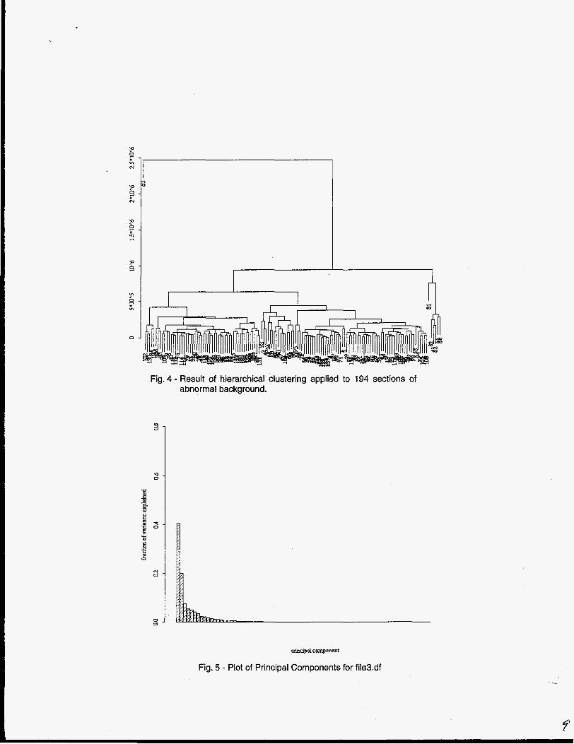
Fig. 4 - Result of hierarchical clustering applied to 194 sections of abnormal background.

n

plinapalcmprmult

Fig. 5 - Plot of Principal Components for file3.df

reasonably well reduced by choosing 3 main clus- ters and 1 outlying cluster of size 1. So, as with kmeans we again find reasonably convincing evi- dence for 4 clusters. Because the hierarchical clustering indicated that case 63 is an outlier, we investigated the cause. First, we used a standard dimension-reduction technique that uses the covariance matrix contain- ing the variances of each feature on the diagonal of the matrix, and the covariances between each fea- ture in the off-diagonals. The dimension-reduction technique then uses eigenvectors of the covari- ance matrix to define a new coordinate system for the data. The first coordinate (called the first principal coordinate (PC)) is the eigenvector corre- sponding to the largest eigenvalue, the second coordinate corresponds to the second largest eigenvalue, etc. If the data is projected in the direc- tion of the principal components, then the variance of transformed data for PC1 is maximum, and the variance of PC2 is next largest constrained to be uncorrelated with PCI. Figure 4 shows the fraction of the total variance of the original data (sum of diagonal entries of covariance matrix) by each PC. Informally, we see that the first two or perhaps the first three PCs contain most of the variance. There- fore, we can see which variables (features) from case 63 contribute most to the first two or three PCs. Also, we can plot PC1 versus PC2 for each case and confirm that case 63 still appears to be an outlier even for this reduced representation of the data (see Fig. 5). By calculating the contribu- tion of each variable to PCl and PC2, we can see that case 63 is an outlier for a surprising reason: the variance of the gamma counts over points 1-20 is unusually high while the mean over points 1-20 is unusually low. To further investigate case 63, we rescaled the data so that all variables would have variance=l . It is a well-known fact that clustering results using covariance matrices can be very dif- ferent from results using correlation matrices, so we wanted to know if case 63 would still appear to be an outlier using the rescaled data. The result was that case 63 continues to appear as an outlier on the rescaled data, but the important variables become the Poisson checks (mean to variance ratios of sections of the data) rather than the vari- ance and mean gamma counts over points 1-20. We currently have no explanation for this behavior.

3) Model-based clustering is a relatively new cluster- ing technique that uses an extended version of hierarchical clustering /15/. The extensions are a Bayesian criterion helps choose the number of clusters, and noise or outliers can be explicitly modeled. Using model-based clustering, again there was evidence for four clusters based on the Bayesian criterion.

To summarize: one of the useful conclusions from the cluster analysis was that one or two true outliers were identified, and a second useful conclusion was a reasonably strong suggestion that the abnormal back- ground contains three clusters, plus a single outlier cluster.

If we have used cluster analysis to define the classes (clusters) of abnormal background, then it is reasonable to develop simple rules involving distance measures to decide if the next section of abnormal data looks reasonably close to an established ("recog- nized") cluster. If not, then either an expert is used to decide if a new cluster for abnormal data should be defined or if the event of interest occurred. In the next section we present classification methods (pattern rec- ognition) that can be used in conjunction with that simple procedure or as a means of discovering better ways to separate the clusters (classes).

3.2 Adaptation and application of several pattern recognition methods

In this section I briefly describe the following pat- tern recognition methods: decision trees, linear dis- criminant analysis, mixture discriminant analysis, flexible discriminant analysis, k-nearest neighbor methods, a new mixture discriminant analysis (written at Los Alamos), and a particular (well-known) neural network called learning vector quantization.

Decision trees. There are several approaches to building decision trees. Figure 6 is a decision tree for file6.df (4 classes and 33 features). The approach I prefer is that implemented in the commercial software CART (classification and regression trees). CART was mentioned in Section 2.1 in connection with MARS. One key issue is how to select one tree from the infi- nitely many possible trees, or how to combine informa- tion from several selected trees. The issue of com- bining information from multiple trees will not be con- sidered here, except to say that simple majority rule voting can be effective. Here we present single trees that were selected from a combination of ad hoc and formal methods. The idea behind CART trees is to build a large tree with many terminal nodes, then to use held-out test data to help select the degree to which the large tree should be pruned back. As is always the case, there is a tendency to overfit the training data (build too many terminal nodes) so it is essential to use held-out test data to counter this ten- dency. Nonterminal nodes are associated with a split criterion such as file6.30 e 30.574 at the root node in Fig. 6. The notation conveys that feature (or predictor) variable number 30 was used and cases with variable 30 < 30.574 travel left through the tree. Variable 30 is the maximum forecast error between points 16 and 25. Such a split criterion is obtained by a trial-and-error method that tries splitting a given node at all feasible

I 3 1 r-

I 4

1 1

Fig. 6 - Decision tree for file6.df with 4 classes, 33 candidate features

breakpoints for numeric variables, or for all possible subset partitions for categorical variables. Other important variables (used in splitting criteria) in the tree shown in Fig. 6 are variable 31 is the position of the maximum error, variable 12 is the slope of the gamma counts over points 1-20, and variable 13 is the error at point 21. Notice that the file6.26 < 4.05 node splits into two nodes that are both labeled class 1. Those labels are the predicted class, so splitting a node into two nodes that will both be predicted to be class 1 cases has no effect on the performance of this tree. However, because the tree was first grown larger and then pruned back, it did have an effect on the larger trees.

The CART software also considers using linear combinations of variables at a given node, but we rarely find that linear combinations of variables are needed. Therefore, this report restricts attention to results using CART-like software that is in the statisti- cal programming language S+, which does not con- sider linear combinations of variables as possible split criteria. The advantages of decision trees include robust with respect to outliers, easy way to allow miss- ing data through use of surrogate splits (each node has second, third, ..., best split criteria that can be used if a case is missing the variable that the best split crite- rion uses), excellent exploratory tool, and simple to use once constructed. For further details, see Ref. 16.

Figure 7 is a decision tree for file5.df (4 classes and 85 features). Variable 82 is the average forecast error over points 21-25. This is a satisfying result because the Neyman-Pearson lemma would suggest that using either a weighted or unweighted sum of the forecast errors over points 21 -25 would be a good dis- criminator. See Ref. 7 for further detail on the applica- tion of the Neyman-Pearson lemma to this type of problem. Variable 55 is the average of the gamma counts over points 29-38 minus the average of the

gamma counts over points 1-20. Variable 44 is the variance of the gamma counts over points 1-20. Recall that case 63 was an outlier largely because of having a very high variance and low mean of the gamma counts over points 1-20. And variable 83 is the slope of the gamma counts over points 1-20. As in Fig. 6, ter- minal nodes are labeled with the predicted class for cases that fall into that node.

p). Linear Discrimi- nant Analysis is the original (dates to 1930s with R. Fisher) pattern recognition method. The assump- tions: for a given class i , the data has a multivariate normal distribution with mean vector hi and covari- ance matrix Z , which is denoted ?li - N(Gi, Z) . That is the mechanisms generating the data for different classes differ only in the mean vector. Under that assumption, Ida is the theoretical best method and is also called Bayes method for that reason. Of course, real data never follow any theoretical distribution exactly, and even if the normality assumption was rea- sonably well met, the assumption of equal covariance matrices remains, as well as the assumption that each class has only one mean vector. Nonetheless, Ida per- forms remarkably well for a variety of real data sets so continues to be a benchmark method.

k - l \ l e a r e s t n ) . The knn method is the simplest to describe. Classify a given case in the testing set according to the classes assigned to the nearest (in the predictor space) k cases in the training set by using majority rule. Break ties randomly. For example, with k=2, if the two near- est cases in the training set have class 1 and 2, then assign class 1 with probability 0.5 and class 2 with probability 0.5. The important issue is choice of metric to compute distances. Also, for extensive use of knn, it is important to restrict the size of the training set

6le5.44 I

4 1

4 1

Fig. 7 - Decision tree for fle5.df with 4 classes, 85 candidate feature

because of the requirement to compute and sort all distances between each test case and all training cases.

Mixture Discriminant Analysis (mda). Mixture Dis- criminant Analysis is a natural extension of Ida, though it is very recent /17L The idea is to allow any number of mean vectors for a given class. A clever application of the EM algorithm (estimation-maximization) is applied to treat the issue that the proportion of cases for a given class that belong to a particular subclass is unknown and therefore is treated as missing in the EM algorithm. The number of subclasses for each class is treated as a “meta-parameter:’ not formally treated in the EM algorithm, but treated by trial and error.

Modified Mixture Discriminant Analysis (mmda). Modified mda was written at Los Alamos in 1995. It is a simpler version of mda that uses kmeans or hierar- chical clustering within a given class to suggest the appropriate number of subclasses (clusters) for each class. Another option to choose the number of clusters is model-based clustering, but we frequently experi- ence computational difficulties with the S+ implemen- tation of it, so have not used it routinely. Having selected a good number of subclass “centers,” we apply the knn approach using the subclass centers with class labels to replace the training data used in the knn approach. That is, class i is represented by ki subclasses, with ki selected by kmeans or hierarchical clustering. Then for a given case in the testing set, the distances from that case to each of the subclass “centers” is computed, and knn is then used with those distances to predict the class of the given case. So at the stage where knn is used, in effect, the subclass centroids replace the training data. That makes knn much faster to use because the number of subclasses is typically much less than the size of the training data.

Neural Network: Learnina Vector Quantization m. The Ivq neural network is similar to our mmda, but with the resulting subclass “centers” replaced by “codebook vectors.” The codebook vectors are selected by trial-and-error, as well as the number of codebook vectors per class. These vectors are not likely to be either an actual training case or a mean vector for a group of training cases because the itera- tive trial-and-error method works in a unique way described, for example, in Ref. 16.

Flexible Discriminant Analvsis (Ma). Flexible Dis- criminant Analysis /18/ is another recent method that exploits the following not-well-known fact. Linear Dis- criminant analysis can be derived by repeated linear regression of the class (viewed as a response) on the predictors. In the first regression, all class=l cases have response=l and all other cases have response=O. In the second regression, all class=2 cases have response=l and all other cases have response=O, and so on. The end result will be esti- mated (scaled) probabilities of each class which can be used to predict class membership. The idea of fda is to replace the linear restriction with any of the regression methods such as described in section 3.2. Our implementation currently uses MARS only.

3.3 Results of the seven pattern recognition methods

In this section we give results of each of the seven pattern recognition methods to file5.df and file6.df and to a simulated data set we call waveform. The wave- form data is described in Ref. 15 and is considered to be a challenging pattern recognition problem for which mda is ideally designed. The theoretically lowest pos- sible misclassification probability is 0.14 for the wave- form data. We used 400 cases to train and 400 cases to test the waveform data.

Recall that file5.df has 4 classes, 85 predictors, and 373 cases. File6.df has 4 classes, 33 predictors, and 373 cases. We presented a selected decision tree for file6.df in Fig. 6 and a decision tree for file5.df in Fig. 7. We created the training and testing set as fol- lows. The number of cases for classes 1-4 were 194, 50, 19, and 1 10, respectively. One half of the cases for each class were randomly selected for training and the other half were used for testing. Here, we record the misclassification rate for the held-out test cases.

Note that for file5.df and file6.df the decision tree performs best, while the mmda and Ivq perform the worst. Recall that the waveform data was designed to showcase mda so it is not surprising that mda does the best on that data. We were pleased with the perfor- mance of mmda on the waveform data however, and though we are disappointed by the poor performance of mmda on file5.df and file6.df, we do believe the method can be competitive on some data sets. We are also surprised by the poor performance of Ivq on file5.df and file6.df. We should emphasize that we did not attempt to fine tune any of the methods. However, we did create file6.df that contained fewer candidate predictors, partly to help all of the classifiers by elimi- nating some possibly unneeded predictors. We do plan to implement ways to fine tune the various classi- fiers. Until we do, the results should be interpreted accordingly. Our intentions in applying and developing pattern recognition methods in such a setting have been to (1) reduce the false alarm rate by sending all alarms into a discriminant function to attempt to sepa- rate true from false alarms, and (2) provide a means to better understand the background data, as in the present case where there appears to be three distinct clusters (plus one outlier) in the class=true cases. To give an example of how we reduce the false alarm rate, consider the result with the decision tree. The “confusion matrix” in Table 2 gives the true class in each column and the tree’s prediction in each row for the cases in the testing set from file6.df.

In Table 2, consider only the cases for which the tree predicted class=4 (the event of interest) when the class was not 4. That occurred 4 times out of 50. That is, of the 50 times that class=4 was predicted, in only 4 cases was the true class not 4. This is an 8% false alarm rate. Therefore, ths overall false alarm rate has been reduced to 8% of the original false alarm rate that is in effect in the rate of creation of the event records. As an important aside, we are beginning to experiment with building multiple trees based on ran- dom resamples (bootstrap samples) of the training set, and then use majority rule to classify. This method is called bagging (bootstrap aggregation). With the wave- form data, the misclassification rate of the bagged tree is about 0.16, which is competitive with any of the methods. Therefore, we believe that tree methods or bagged-tree methods show great promise for a wide range of data sets. Also, we should point out that the reduction in false alarm rate does not come for free. We also have 109 cases that the tree predicted to be class=l (not the event of interest) and of those 109 there were 9 class=4 cases. That means we have approximately a 10% failure-to-detect probability. If the failure-to-detect probability must be reduced, then we would suggest a version of Ida so the user can select the thresholds accordingly.

TABLE 2. Confusion matrix for the tree classifier for file6.df. Column is true class. Row is predicted class.

2 0 23 0 0

4. Conclusions

There is much current research in the area of com- bining information, which I informally defined to include both data and judgment. Some degree of infor- mation combination is done in nearly any data analy- sis. The particular situation considered in Sections 2 and 3 assumed that we have more data than judg- ment, and wish to use the data in a somewhat explor- atory mode in order to refine our judgment. For example, we want to learn how frequently the data looks abnormal, how many different types (clusters or classes) of abnormal data is present, and how well we can separate the abnormal but not the event of interest data from the event of interest data. With that goal in mind, I have presented a suite of approaches to mod- eling and forecasting the ordinary background to enhance the method used for flagging unusual back- ground that must be further analyzed by pattern recog- nition. The suite ranged from the most basic to the most modern and each method will have some suit- able domain of application. In this report the best

13

b > -

c

modeling method was defined to be the one that had minimum average squared error for the held-out testing set. Using that definition, the simplest forecast- ing methods such as the exponentially weighted mov- ing average is best for the one main data set analyzed. That will not always be the case, so it is important to have a suite of modeling tools available.

Also, I presented a study of the application of pat- tern recognition to the sections of abnormal data. We anticipate that many surveillance settings will operate in a similar manner: monitor a subset of key time series and keep a short buffer of data available at per- haps higher resolution for all time series that can be further analyzed when “suspicion level” is raised as judged by some alarm threshold. Follow all alarms with “anomaly resolution” to attempt to assign causes to each alarm. For example, note from the confusion matrix shown in Section 3 that of the 25 class=2 cases, 23 were correctly identified. With a little fine tuning of the classifier we expect nearly all of the class=2 events could be easily identified. Of course in this setting the operators already know that the cali- bration event caused the alarm that caused the cre- ation of the event record, but the idea is still quite useful here and should be very useful in other settings. It can also sometimes be of interest to better charac- terize the background also, and in our case there was strong indication of three distinct clusters plus one out- lier. We believe that this approach will have multiple applications.

5. References

1. J. Pill, ”The Delphi method: Substance, context, a cri- tique and an annotated bibliography,” Socio-Econ. Plan. Sci. 557-71, (1971).

2. D. Geman and S. Geman, “Stochastic relaxation, Gibbbs distributions and the Bayesian resotration of images,” IEEE Trans. Pattern Anal. Machine Install. 121721 -741, (1 984).

3. P. A. Morris, “Combining expert judgments: A Bayesian approach,” Management Science 23:679-693 (1 977).

4. A. f? Dempster, “Probability, evidence, and judgment,” Bayesian Statistics 2:119-131, (1 985).

5. G. E. P. Box, G. M. Jenkins, Time Series Analysis: Forecasting and Control, 3rd Ed. (Holden-Day, San Francisco, 1994).

6. S. Bleasdale, T. Burr, A. Coulter, J. Doak, B. Hoffbauer, .D. Martinez, J. Prommel, C. Scovel, R. Strittmatter, T. Thomas, A. Zardecki, “Knowledge Fusion: Analysis of Vector-Based Time Series with an Example from the SABRS Project,” Los Alamos National Laboratory report LA-1 2931 -MS, April 1995.

7. S. Bleasdale, T. Burr, J. Scovel, R. Strittmatter, “Knowl- edge Fusion: An Approach to Time Series Model Selec- tion Followed by Pattern Recognition,” Los Alamos National Laboratory report LA-1 3095-MS ( 1 996).

8. T. Burr, “Prediction of Linear and Nonlinear Time Series With an Application in Nuclear Safeguards and Nonpro- liferation,’’ Los Alamos National Laboratory report LA-12766-MS, April 1994.

9. J. Friedman, “Multivariate Additive Regression Splines,” Annals of Statistics, 1991

10. T. Burr, R. Strittmatter, “Knowledge Fusion: Comparison of Fuzzy Curve Smoother to Statistically-motivated Curve Smoothers,” Los Alamos National Laboratory report LA-13076-MS (1996).

11. L. Wang, J. Mendel, “Generating Fuzzy Rules by Learn- ing from Examples”, IEEE Transactions on Systems, Man, and Cybernetics, Vol. 22, No. 6, NovIDec 1992,

12. P. Robinson, “Nonparametric Estimators for Time Series,” Journal of Time Series Analysis Vol. 4, No. 3,

13. T. Burr, J. Doak, J. Howell, D. Martinez, R. Strittmatter, “Knowledge Fusion: Time Series Modeling Followed by Pattern Recognition Applied to Unusual Sections of Background Data: Los Alamos National Laboratory report LA-13075-MS (1996).

14. J. Hartigan, Clustering Algorithms (Wiley, New York,

15. J. Banfield, A. Raftery, “Model-based Gaussian and non-Gaussian clustering,” Biometrics, Vol. 49, No. 3, pp 803-822 (Sept 1993).

16. L. Brieman, J. Friedman, R. Olshen, C. Stone, Classifi- cation and Regression Trees (Wadsworth & Brooks, Monterey, California, 1984)

17. T. Hastie, R. Tibshirani, “Discriminant Analysis by Gaus- sian Mixtures,” Journal of the Royal Statistical Society-B (1 994)

18. T. Kohonen, ‘The self-organizing map,” Proceedings

19. T. Hastie, R. Tibshirani, A. Buja, “Flexible Discriminant Analysis by Optimal Scoring,” Journal of the American Statistical Association, Vol. 89, No. 428, pp. 1255-1270 (1994).

pp.1414-1427.

pp. 185-207.

1975).

IEEE, 78, pp. 464-1480

6. Acknowledgement

The author thanks the Knowledge Fusion Project Team: S. Bleasdale, A. Coulter, J. Doak, B. Hoffbauer, D. Martinez, J. Prommel, C. Scovel, R. Strittmatter, T. Thomas, A. Zardecki.

This work was supported by the US Department of Energy, Office of Nonproliferation and National Security.