Solvency II - An important case in Applied VaR

Alfredo D. Egídio dos Reis1, Raquel M. Gaspar2, and Ana T. Vicente3

Abstract:

Value-at-Risk (VaR) is an extremely popular risk measure and many financial companies

have successfully used it to manage their risks. Recent developments towards a general

single European financial regulation, lead to a great increase in the use of VaR. At least,

for European Bank and Insurance industry, VaR is no longer an optional risk

management tool, but it became mandatory.

In this chapter we focus on the Insurance business and discuss the use of VaR as it has

been proposed in the context of the Solvency II (undergoing) negotiations. Our goals are,

on the one hand, to present the underlying assumptions of the models that have been

proposed in the Quantitative Impact Studies (QIS) and, on the other hand, to suggest

alternative VaR implementations, based upon estimation methods and firm specific

characteristics. Our suggestions may be used to develop internal models as suggested in

Solvency II context. Finally, we analyze the case a of Portuguese insurer operating in the

motor branch and compare QIS and internal model VaR implementations. In our concrete

application, (one year horizon) capital requirements are similar under the two

alternatives, allowing us to conclude for the robustness of the models proposed in QIS.

Keywords: Value-at-Risk, Financial risk regulation, insurance regulation, Solvency II

1 CEMAPRE and ISEG, Technical University of Lisbon. Partial financial support from FCT-Fundação para a Cieência e Tecnologia (Programme FEDER/POCI 2010) is gratefully acknowledged. 2 ADVANCE and ISEG, Technical University of Lisbon. Support for this author was provided by FCT under grant PTDC/MAT/64838/2006. 3 ISP-Instituto de Seguros de Portugal (Portuguese Insurance and Pension Fund Supervision Authority)

1

1. Introduction

Insurance is a risky and a risk business and insurance companies’ role, in the economic

activity as an institutional investors, is increasingly important.

On the one hand and given the purpose of its business, an insurer is a risk taker by selling

insurance. So, to be able to survive in their industry, insurers needs to make sure they are

able to satisfy the responsibilities assumed towards their clients. To fulfil that purpose an

insurer needs not only, to appropriately evaluate the risks at stake charging appropriate

insurance premiums, but also to calculate the amount of capital that should be kept in

order to face other losses that, in some situations, can be quite adverse. Naturally, such

capital requirements are based on risk taking and depend upon the concrete nature and

amount of risks a specific insurer covers. Risks that can be associated with the insurance

firm core activity are many times called insurance risks. Examples of such risks are the

following: possible wrong assessment of the risks insured (premiums charged may not be

enough to cover the assumed responsibilities), defaults from their clients (in paying

agreed future premiums); or counterparty risk from re-insurers (other entities whom they

sold their risks to and may default on their contracts leaving the insurance company with

the original obligations they thought they no longer had as they had been resold).

On the other hand, an insurer is an investor and a natural player on financial or capital

markets. As any investor, an insurer’s portfolio typically consists of various assets of

different types with different risk profiles. The assets portfolio of an insurer include all

types of products, from simple deposits, to stocks, bonds, investment funds units, real

estate investments and various types of derivative products on a variety of possible

underlying. These risks should also be accessed, both in nature and amount, and taken

2

into account when computing capital requirements. These are risks that do not result

directly from the insurer’s core activity but from the fact that cash-flows resulting from

that activity are invested in risky financial products. They are, therefore, globally called

market risk.

The insurance sector carries significant importance in Europe. On voluntary, as well as on

statutory basis, it provides cover against various risks facing the citizens, corporations

and other organizations. In addition, collecting long-term savings of millions of

Europeans, it is the largest institutional investor on EU stock exchanges. An appropriate

prudential framework for insurance is therefore of extreme importance. Recent

catastrophic events – whether natural or man-made – have highlighted the significance of

having a stable and solvent insurance sector.

The previous EU solvency system, introduced in the 1970s, was conceived in a period

when the general economic features, as well as insurance practices, were different.

Capital requirements of insurance undertakings were determined based on simple ratios

that were calculated as percentages of risk exposure measures (e.g. technical provisions,

premiums or claims). Nowadays, insurance companies are faced with a different business

situation with increasing competition, convergence between financial sectors as well as

international dependence. At the same time insurance, asset, and risk management

methods and techniques have been significantly refined. The recent economic downturn

and volatile financial markets have also put the insurance sector solvency and risk

management under significant pressure.

The inadequacy of the old solvency system started to be discussed in 1998, when the

European Commission acknowledge the need of “enhancing consumer confidence by

3

promoting full financial market integration while ensuring high levels of consumer

protection” [European Commission (1998)] and initiated several changes to the existing

directives, leading the European control authorities (of the insurance business) into the

development of a new solvency project. For further details, on the background and

international context of the new project, we refer to Linder and Ronkainen (2004).

The new European Solvency Project was organized in two phases: In the first phase,

known as Solvency I, fundamental arrangements were specified, a general framework

was defined, and several studies were ordered by the European Commission. The most

well-known studies are the KPMG (2002) study and what became known as the Sharma

(2002) Report. For a survey on all studies ordered by the European Commission and their

recommendations see Eling, Schmeiser and Schmit (2007). This first phase ended during

2003 and its recommendations became effective as of January 2004.4 In a second phase,

called Solvency II, these fundamentals are being developed into specific rules and

guidelines. This project follows in spirit the so called Basel II agreement, established and

already in application in the European banking industry. The solvency working group is,

thus, moving towards convergence of insurance and banking regulatory systems. Still, a

significant difference between the two is that Solvency II focuses more heavily on a

holistic risk management approach rather than on management of single risks

independently. The Solvency II project is not yet established, as is still under scrutiny by

different supervisory authorities in each EU country and changes may still occur. In fact,

this input capacity was specifically sought by the EU as part of the regulatory

development process. See European Commission (2003). Value-at-Risk (VaR) has

4 Solvency I addressed many of the coordination issues across regulatory bodies and provided an initial rules-based set of capital requirements (see EU Directive 2002/13/EC for non-life insurers and EU Directive 2002/83/EC for life insurers).

4

emerged as a key instrument and will continue to be so. This study discusses the use of

VaR, as it has been proposed in the context of the Solvency II and it is organized as

follows. In the next section, Section 2, we make a summary presentation of the Solvency

II project and discuss the possibility insurance companies have of developing their own

internal models when computing capital requirements. In Section 3 we do a critical

presentation the standard method for capital requirement calculation suggested in

Solvency II and put into practice by the Third Quantitative Impact Study (QIS3)5. We

highlight the standard method assumptions and propose alternatives that could be useful

in building internal models. In Section 4, we consider the case of an insurer operating in

the Portuguese motor branch. For this concrete insurer we compute (one year) capital

requirement both directly applying the QIS3 rules and thought an internal model that

takes into account our suggestions. In the last section we finish the work by addressing

final remarks and criticisms on the models used and results obtained.

2. Solvency II and QIS3

Traditional European solvency systems, monitored by control authorities in each country,

were based on solvency margins and technical reserves for each branch. Even in the

current system – Solvency I – the solvency level depends only on the amount of

premiums or claims, and there is no relation with capital requirements and risk taken.

Solvency II aims to be a major improvement over the previous schemes. For the first time

a solvency scheme acknowledge the important role insurers play in the world financial

markets, and has the ambition of taking into account the financial market risk associated

5 Several quantitative impact studies have been put in place by the CEA-Comité Européen des Assurances by request of CEIOPS-Committee of European Insurance and Occupational Pension Supervision. Their purpose is to study the impact of the introduction of Solvency II rules.

5

with insurers’ investments – the market risk. In addition, Solvency II also acknowledges

the business of risk is risky in itself, classifying and taking into account various insurance

risks: underwriting risk, counterparty risk, operational risk. Similarly to its banking

industry counterpart, the Basel II project, Solvency II has been structured along three

main objectives – called the three pillars. Pillar I defines the financial resources that a

company needs to hold in order to be considered solvent. Two thresholds are defined, the

first called the Solvency Capital Requirement (SCR), and another lower threshold called

the Minimum Capital Requirement (MCR). The SCR level is a first action level, that is,

supervisory action will be triggered if resources fall below its level. The MCR is a severe

action level by the control authority, which can include company closure to new business.

While Pillar I focus on quantitative requirements Pillar II defines more qualitative

requirements and supplements the first. For instance, it defines the framework of

intervention of the supervisory authority . Finally, Pillar III addresses issues such as risk

disclosure requirements, transparency or free access to information.

In this chapter our main focus is on the quantitative aspects of Solvency II and thus, on

Pilar I and, in particular, in evaluating the SCR. For the calculation of the SCR, Solvency

II proposes a standard (simple) model but encourages the development of internal models

that would provide a better adequacy to the kind, spread and amount of risks taken by

each insurer. This is underlined by Ronkainen et al. (2007). Still, as mentioned in

Liebwein (2006), any internal model alternative would have to accomplish legal

requirements, provide greater added value to shareholders when risk management

processes are included, and be subject to approval by the control authorities.

6

On what concerns technical reserves, i.e. those directly connected with insurance risks,

the premium reserves and the reserves for pending claims must be computed separately.

In the absence of an active market, the technical reserves must be estimated and a risk

margin must be added. For the estimating procedure a probability distribution of the cash-

flows must be estimated, the mean value of this distribution will then be used as an

estimate. This is known as the Best Estimate. The risk margin works as loading and

intends to cover the volatility of the risk factors, the uncertainty of the best estimate, the

risk associated to the insurance portfolio of the company and natural estimation errors,

from the model and its parameters. It is also used to compute a market value for the

insurer or branch. The Best Estimate will be used as an approximation to the future costs

that the insurer is expected to cover, and this will be the basis of the computation of its

capital needs. For such calculation the insurer must have reliable and organized loss past

data to allow the use of proper statistical methods. For instance, claim payments of

accidents occurring in one year develop along one or more future years. Typically, we

need to fill out an empty triangle with properly estimated values.6 The discounted sum of

the estimated claim payments of each occurrence year will be our estimate for the loss

reserves for that year. There are several methods to compute the future payments; the

most popular is the so called Chain Ladder. For more details on this and other methods

please see Taylor (2000). Further discussion on this subject can also be found in Mack

(1994) and Verral (1994).

6 An example is shown in Table 3 with the data of our application. There, we can see, for instance that losses occurred in 2001 can develop until 2006 or even more, that needs to be estimated as well. Along each line we have payments for losses occurred in each starting year, here the values are incremental payments.

7

Market risk can, in a more straightforward way, be computed from market quotes. These

risks are also not related with each insurance firm, instead they are related to specificities

of particular classes of assets. So, one can think of general rules that may apply to such

classes of assets and that should be implemented by all firms.

Whether implied from market quotes or estimated, future uncertainty should be evaluated

using a risk measure. Although the European working parties suggest the use of both the

VaR measure and the Conditional Tail Expectation measure – also known as Tail VaR –

at the moment only the VaR measure is considered as a standard 7.

Definition 1: Let X be a random variable representing the values of an asset or a return

rate for instance. The Value-at-Risk, denoted as , is defined as VaRα

( ){VaR inf : Pr100% x X x αα×= ∈ > ≤ }

(1)

In the following we critically present the standard model proposed by the Committee of

European Insurance and Occupational Pension Supervision (CEIOPS), as it stands in the

latest Quantitative Impact Study (QIS3) and discuss possible alternatives for

implementing VaR, whenever we feel it is appropriate.

One first point we would like to make is that the VaR measure makes no assumption

concerning the distribution of the random variable we are interested in computing the

quantile. Thus, various approaches exist, some called parametric and based upon

7 In any situation, we will stick to the use of VaR as it is the only risk measure considered as standard in the context of Solvency II. We notice, however, that VaR as a risk measurement has been quite criticized, in the financial literature. A subtle technical problem is that VaR is not sub-additive. That is, it is possible to construct two portfolios, A and B, in such a way that VaR (A+B) > VaR(A)+VaR(B), which contradicts the idea of diversification. A theory of coherent risk measures exists outlining the properties we would want any measure of risk to possess. As opposed to VaR, Tail VaR is a coherent risk measure. For further details on this subject we refer to the canonical paper on the subject: Artzner, et al (1999).

8

assumptions about the underlying distributions – the most commonly used is the

Gaussian distribution, others based upon empirical distributions. This last approach

requires collecting (usually historical) past information on the random variable we are

interested in and observing the appropriate quantile and is, thus, known as historical

approach to VaR. Both parametric and historical approaches to implementing VaR have

their own advantages and disadvantages. On the one hand, any parametric model requires

parameter estimation which require choosing the appropriate estimation method and

evaluating the ability of the model to explain the data. Furthermore, many of the variables

we are interested in are far from the most well known parametric distributions (and

clearly far from Gaussian), indicating a historical approach could be best. The historical

approach to determining VaR is a nonparametric approach that requires no direct

estimation. On the other hand, however, and especially because we are concerned with

extreme events the amount of historical information one may need to collect in order to

capture well the tail behavior of a distribution can be substantial. Also, we may want to

consider the possibility that some extreme events that have not yet occurred in the past,

may occur in the future. This advocates in favor of parametric methods. Probably the

sensible attitude is to use either both methods – choosing the worst case scenario – or a

mixture of them. For a detailed discussion on various VaR implementations we refer to

Linsmeier and Pearson (1996) and Jorion (2001).

As we will see, the standard model, as proposed in QIS3, relies considerably on a

parametric Gaussian implementation of VaR. We propose, instead that, provided there is

enough information on the relevant variables – which is typically the case at least on what

concerns with financial data – an historical approach will be more accurate evaluating

9

VaR. The QIS3 computations rely considerably on the following VaR result for normally

distributed random variables.

Result 2: Suppose you have N random variables, for , all normally

distributed with mean zero and variance . Let Y define a linear

combination of the random variables , where the ’s are constants. We denote

shortly by the VaR of order of each random variable. Then the VaR of Y ,

nX 1,2 ,,n =

1 nN

nnw X

=∑

N

nσ =

nwnX

αVaR( )nX

, 1

) VaR( )VVaR(N

ij i j i ji j

Y w w Xρ=

= ∑ ar( )X , (2)

where all VaR are computed for the same probability . α

For the remaining of this section we discuss in detail the implementation of both

alternatives. The various risks were divided according to their nature into: market risk,

counterparty risk, underwriting risk and operational risk. The final assessment of the

capital requirement is obtained by a risk aggregation, considering all the above

mentioned risks.

We aim at applying the methods here discussed to an insurer operating in the motor

branch. We, therefore focus, as far as insurance risks are concerned, on risks specific of

that branch. Also, we do not include in our study catastrophe risk as appropriate data

would be hard to find and its complexity is beyond the scope of our application. As far as

market risks are concerned, we refrain from discussing the impact of two important

classes of assets in capital requirements: risk management assets (such as derivatives) and

real estate assets. Both these classes of assets were absent from our concrete insurer

10

portfolio, but deserve special attention in QIS3. For details on how to include risks or

these types of assets not mentioned in this study we refer to CEIOPS (2007a,b,c).

2.1 Market Risk

When evaluating market risk we are mainly concerned with measuring the impact that

changes in the market value of various assets have in the overall investments that insurers

do when applying the cash-flows of its activity, in risky financial markets. The standard

approach suggested in QIS3 relies on two key assumptions: (i) that financial returns are

normally distributed and (ii) that such a distribution is static, i.e., is does not evolve over

time. Both these assumptions have been widely studied in the financial literature and it

has been found enough evidence allowing us to clearly reject any of them. See, for

instance, Cont (2001). Moreover, capital requirements are computed assuming a static

portfolio, i.e. that a portfolio does not change over time. Good risk management practice,

however, requires rebalancing the portfolio periodically. There is a clear inconsistency

between accessing risk (via capital requirements) assuming a static portfolio when good

risk management lead to a dynamic portfolio. The best we can suggest to overcome this

difficulty is to periodically re-evaluate the capital requirements estimation; with a

periodicity similar to the periodicity each firm changes their portfolio. We now look

deeper into each asset class, present the QIS3 standard model suggestion and propose our

alternative. For exact formulas concerning the QIS3 approach we refer to CEIOPS

(2007a,b,c).

As far as equity risk is concerned, QIS3 divides it into specific and systematic risk. As

the first type of risk can be eliminated in a well diversified portfolio, QIS3 considers it as

concentration risk (and not equity risk). Having to deal only with the systematic part of

11

equity risk, QIS3 relies on two indices: a “Global index” that includes all stocks from

European countries and other global markets, and a second index called “Others index”

where the remaining countries should be included as well as any non quoted stocks

(irrespective of their country). Based upon collected historical information and assuming

a Gaussian distribution with mean zero for each index returns, QIS3 estimated each index

obtaining -32% and -45%, for the Global and Others indices, respectively.

Also, QIS 3 suggests the use of a correlation of 0.75 between the two indices and

equation

99.5%VaR

(2) to take into account the diversification effect across indices.8

An insurer is exposed to interest rate risk via all assets and liabilities whose value is

sensitive to changes in the term structure of interest rates. Example of such assets and

liabilities are fixed-income investments, insurance liabilities, loans, etc. The QIS3

standard model assumes that default-free interest rates (also known as zero-rates)

maturing each year from 1y to 20y are independent variables. For each of these variables,

QIS3 estimates both with and , assuming that changes in

rates of any maturity are normally distributed with mean zero. Even though the

independence across maturities and the Gaussian assumption are questionable, the

proposed standard method allows considering the risk of various movements of the term

structure taking into account that rates with different maturities have different volatilities.

Also, computing two quantiles for each variable makes sense has an insurer may be more

exposed to the risk of interest rates increasing, or decreasing. Finally, when implementing

the standard method each insurer must decompose the payoffs of each interest rate

VaR 0.005α = 0.995α =

8 To the best of our knowledge, only the “Global Index” volatility was estimated based upon quarterly data on the MSCI Developed Markets index, from 1970 to 2005. The “Others index” volatility and correlation between both indices are add-hoc values suggested in QIS3.

12

sensitive asset or liability to match the yearly maturities up to 20 years9. Table 1 presents

QIS3 VaR estimates for changes in zero rates of different maturities10.

VaR \ T 1 2 3 4 5 6 7 8 9 10-15 16 17 18 19 20+

0.005α = 0.94 0.77 0.69 0.62 0.56 0.52 0.49 0.46 0.44 0.42 0.41 0.40 0.39 0.38 0.37 0.995α = -0.51 -0.47 -0.44 -0.42 -0.40 -0.38 -0.37 -0.35 -0.34 -0.34 -0.33 -0.33 -0.32 -0.31 -0.31

Table 1 :VaR for changes in zero rates of several maturities (QIS3 estimates).

Currency risk arises from the level of volatility of currency exchange rates. An insurer is

exposed to that risk whenever she directly invests in foreign currencies or when some of

her assets or liabilities are denominated in a currency other than its home currency. Once

again, the standard model in QIS3 assumes that changes in exchange rates follow a

Normal distribution with zero mean. Supposing quotes are in a (Foreign/Home) form,

whenever a foreign currency depreciates the mentioned ratio increases. So, provided we

subtract the liabilities to the assets denominated in foreign currency (i.e. we consider only

the net asset value), adverse movements are measured by VaR with . QIS3,

considered only the variation of the euro relative to a index of foreign currencies and

estimates, therefore, only one which turned out to be of 20%.

0.005α =

VaR 11

Spread or credit risk is part of the risk an insurer is exposed to via its investments in

financial markets. It is associated with the credit worthiness of some financial products

issued by corporations. The typical example are corporate bonds whose value is lower

than a (otherwise equivalent) government bond because it may happen that the

corporation fails to pay some of the coupons or capital. Credit risk can be measured by

9 The QIS3 recommends for maturities longer than 20 years, the use of the 20 year VaR. 10 These estimates we obtained using German monthly zero-coupon rates, from 1y to 10y maturities since 1972 and also extracted from daily data European Swaps with 1y,5y,10y,15y,20y, 25y and 30y, since 1997. 11 This estimation was performed using monthly exchange rate quotes towards the euro from 1958 to 2006, excluding the Bretton-Woods period (1992-2001). The foreign currencies considered were the US dollar, the British pound, the Japanese yen, the Swedish crone, the Swiss franc and the Australian dollar.

13

the difference in yields between corporate and government bonds. Such a difference is

called the credit spread. Clearly, in the same way interest rates vary across maturities

also credit spreads will do so, originating what is known as a credit curve or credit spread

terms structure. Moreover, naturally, credit spreads vary across ratings: products with less

credit risk (higher rating) will have lower spreads than those with lower credit worthiness

(lower rating). The QIS3 standard approach takes both these facts into account and

analyse various pairs of (duration12, credit rating class). Nonetheless, credit spreads of

each pair are taken as independent random variables. For an insurer the risk is that their

investments will be worth less due to a decrease in credibility, which is the same as an

increase in credit spreads. Thus, the appropriate figure we are looking for when trying to

access this risk is a VaR with . 0.995α = Table 2 presents such a VaR for some

combinations of duration/credit class13.

Table 2: VaR for assets with different durations and credit spreads. (Based upon QIS3 calibrations).

99.5%VaR 2 4 6 8 10 12 14

AAA or AA 0.5% 1% 1.5% 2% 2.5% 3% 3.5% A 2.06% 4.12% 6.18% 8.24% 10.30% 12.36% 14.42%

BBB 2.25% 4.50% 6.75% 9% 11.25% 13. 05% 15.30% BB 6.78% 13.56% 20.34% 27.12% 27.12% 27.12% 27.12% B 11.2% 22.4% 33.6% 33.6% 33.6% 33.6% 33.6%

CCC 22.4% 44.8% 44.8% 44.8% 44.8% 44.8% 44.8% Unrated 4% 8% 12% 16% 20% 24% 28%

The last risk we must refer to before aggregating all market risks is concentration risk.

In QIS3, the definition of concentration risk is restricted to the risk regarding the

accumulation of exposures with the same counterparty also called name. It does not

12 Here we refer to the Fisher-Weil Duration measure that can be interpreted as an average payment time of a cash-flow stream paid at several points in time. For further detail we refer to Weil (1973). 13 QIS are not presented as in Table 2. Instead, they present two separate functions, a function dependent upon the rating class and an independent function that depends upon duration alone. The final VaR measure is then obtained multiplying the two functions. We believe the above table allows a better understanding of the risks at stake and refer to CEIOPS (2007c) for further details.

14

include other types of concentrations such as geographical concentration, industry sector

concentration, etc. All entities belonging to the same group are interpreted as the same

name. An add-hoc concentration threshold is defined based upon the credit rating of each

product: for products with A or higher rating the threshold is 5% for the insurer total

assets value while for products with lower rating is 3%. QIS proposes an excess expose

measure based upon those thresholds and VaR corrections that should be preformed when

the insurer’s assets are not well diversified enough. Most insurers do have well

diversified portfolios, so it is quite common to obtain zero concentration risk. This is the

case in our case study, we refer to CEIOPS (2007a) for calibration details and actual VaR

corrections. Finally, to compute the overall market risk VaR, QIS3 simply suggests the

use of equation (2) with an add-hoc correlation matrix14 and take into account each asset

class weight in terms of the total assets considered in the market risk analysis.

We now briefly discuss an alternative, to the QIS3 standard VaR, for measuring all

market risks. In the case study we will use this alternative as our Internal Model. Our

suggestion relies on two main ideas: (i) to consider the historical approach to VaR when

evaluating market risks and (ii) to use information each insurer has easy access to its own

current portfolio composition. The historical approach to VaR is considered by many

authors as “the simplest and most transparent method of calculation” [Dowd (2005)]. It

involves running the current portfolio across a set of historical asset values and to build a

historical return distribution to obtain the relevant percentile (the VaR). The key aspect

here is that we do not assume a normal distribution of asset returns. Moreover, using the

insurer specific portfolio composition, we focus on the exact risks the insurer take and not

14 The exact correlation matrix suggested in QIS3 is presented in Table 4 where it is compared with an alternative matrix estimated considering our case study Insurer specific portfolio.

15

all the risk it could take. The main drawbacks that could be pointed out are the

requirement for a large market database and the computationally intensive calculations.

The first is hardly a problem in the concrete case of market risks as long financial time

series are typically available. The second drawback depends upon the complexity of the

insurer portfolio and can be overcome with a good computer program. Our suggestion,

for computing market risk takes into account the current issuer portfolio and, for each risk

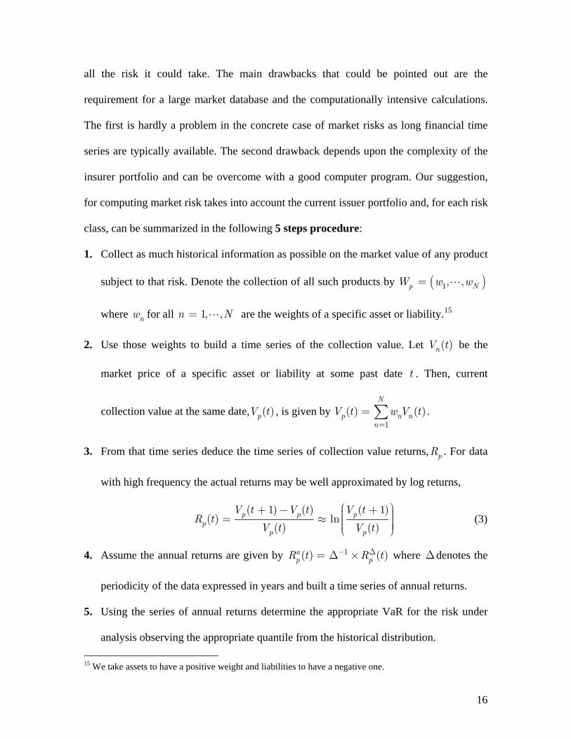
class, can be summarized in the following 5 steps procedure:

1. Collect as much historical information as possible on the market value of any product

subject to that risk. Denote the collection of all such products by ( )1, ,p NW w w=

where nw for all , ,1n N are the weights of a specific asset or liability.= 15

2. Use those weights to build a time series of the collection value. Let ( )nV t be the

market price of a specific asset or liability at some past date t . Then, current

collection value at the same date, ( )pV t , is given by )n t . 1

( )N

p nn

V t w=

= ∑ (V

3. From that time series deduce the time series of collection value returns, pR . For data

with high frequency the actual returns may be well approximated by log returns,

( 1) ( ) ( 1)

( ) ln( ) ( )

p p pp

p p

V t V t V tt

VR

V t t

⎛ ⎞+ − + ⎟⎜ ⎟⎜= ≈ ⎟⎜ ⎟⎟⎜⎝ ⎠ (3)

4. Assume the annual returns are given by p t where Δdenotes the

periodicity of the data expressed in years and built a time series of annual returns.

1( ) ( )ap tR R− Δ= Δ ×

5. Using the series of annual returns determine the appropriate VaR for the risk under

analysis observing the appropriate quantile from the historical distribution. 15 We take assets to have a positive weight and liabilities to have a negative one.

16

To aggregate the total market risk, estimate the correlations between each type of risks

from the various time series determined in 5. Then, using the estimated correlations and

the previously obtained VaR for each risk, we apply equation (2) and obtain the SCR for

market risk using.

We note that our Internal Model approach to estimate market risk is similar, at least in

spirit, to the ideas underlying the QIS3 proposal. To be more concrete, when dealing

with interest rate risk, we recommend considering several points of the interest rate term

structure and computing the VaR for each of them. The difference is that we believe the

relevant points should be chosen taking into account the durations of the assets and

liabilities exposed to interest rate risk in the insurer current portfolio. For credit spread

risk, we also suggest grouping the products according to their rating and duration.

However, taking a historical VaR approach would mean estimating a VaR for each pair

(duration, rating) based upon past yield changes. Finally, we notice that using this

approach it makes no sense to define a concentration risk as we have not considered only

the systematic risk of each product but its actual total risk16 We now go on analyzing

insurance risks, i.e. risks that are more related to an insurer’s core activity.

2.2 Counterparty Default Risk

This is the risk of default of a counterparty to risk mitigation contracts like reinsurance

and financial OTC17 derivatives. In terms of the amounts at stake, reinsurance

counterparty risk tends to be the most important. In our case-study it is also the only one.

Here we analyze only reinsurance counterparty risk. If case of default from a reinsurance 16 Due to space restrictions we do not describe in detail our approach to each of the market risks. Instead, we present the main steps and refer to Vicente (2008) for further details. 17 Over-the-Counter (OTC) derivatives are bilateral contracts traded outside exchanges and thus subject to counterparty risk.

17

counterparty, the insurer will incur in replacement costs (RC), which can be evaluated as

the sum of the technical reserves of the ceded reinsurance plus the extra (previously paid)

premium minus any recoveries. QIS3 assumes zero recovery in case of default and

estimates probabilities of default (PD) for different reinsurance rating classes. The rating

classes are the same as those in Table 2, except that the first two, AAA and AA, come

separated and the last two come merged. The figures (in %) in a decreasing rating scale

come, 0.002%, 0.01%, 0.05%, 0.24%, 1.2%, 6.04% and 30.41%, respectively. The VaR

for this risk is computed in three steps: (1) calculation of the so called Herfindahl index18,

(2) calculation of capital requirement per counterparty and (3) aggregation. The final

formula for the VaR depends on an implicit correlation of counterparty default. In our

case-study the correlation is 1 and the formula is give by

. We refer to CEIOPS (2007a) for details on this method

or on how QIS3 handles derivative related counterparty risk. Given the complexity of

counterparty risk modeling we suggest no Internal Model to the QIS3 approach.

min{100VaR RC PD;1}× ×=

2.3 Underwriting Risk

This sort of risk arises directly from the nature of the insurance activity. In the case of

non-life insurance, it basically includes premium risk and the reserve risk.19 On what

concerns premium and reserve risk, QIS3 standard approach rely on two measures: a

premium volume measure (PVM) and a reserve volume measure (RVM) and in

evaluating the variations of such measures to compute their volatilities. For the premium

risk the QIS3 suggestion are either to directly observe the PMV from the insurer’s 18 The Herfindahl index is a measure of the size of firms in relationship to the industry and an indicator of the amount of competition among them. 19 Catastrophe risk (Cat risk) is also considered as underwriting risk. However, as previously mentioned, we do not analyse this risk in the context of this study.

18

estimate of the premiums for next year, net of reinsurance or to consider an increase of

5% on the actual net premiums. Even though 5% is an add-hoc, lack of information

makes this second option quite used in practice. This will also be the option we will

choose for our case-study. QIS3, then suggests to obtain the PVM volatility, , by the

well known Bühlmann and Straub’s credibility formula:

prσ

2 2(1

VM+

)prI Mc c σ= + −σ σ

where is the insurer’s sigma, is the market sigma and c is a constant dependent

upon the sample size n ( if and otherwise).

Iσ

σ

Mσ

/ (

Mσ

4)c n n= + 7n ≥

Iσ

0c

P

= 20 QIS 3

uses a fixed value of 10% for , and suggest to be computed by (historical)

estimation, calculating a (weighted) sample standard deviation of the loss ratio, annual

claims cost over premiums net of reinsurance. For the reserve risk, their suggestion is to

use the figure for the loss reserves from the insurer’s last year balance sheet as RVM.

This is an amount supervised by the control authorities. QIS3 computes the RVM

volatility, , first computing the volatility of the line of business third party liabilities

and of the other classes and then aggregating it. QIS3 recommends the use of 12.5% and

7.5%, respectively, for the two mentioned volatilities. Finally, the overall underwriting

VaR is obtained using the sum of the volume measures VM and to

the following formula,

res

VM R=

( ){ }2

99.5%N ln( 1)

2VaR with ( ) 1

1

eVMf fσ

σ σσ

+

= =+

−

/

(4)

where stands for the 99.5 percentile of a standard normal distribution and σ is

an overall volatility given by . The function

99.5%N

2 2( )pr resPVM RVM VMσ σ σ= × × ×

20 See Buhlmann and Gisler (2005) for more details on the credibility formula.

19

)(f σ implicitly assumes that the underwriting risk follows a lognormal distribution and

is such that, for a small and medium size σ , gives roughly 3σ .

Next, we discuss alternative procedures, that may be used an Internal Model, to evaluate

the underwriting risk. For premium risk we consider a sum of loss and expense ratios,

called combined ratio CR, . The loss ratio (incurred losses and loss-

adjustment expenses divided by net earned premium) is added to the expense ratio

(underwriting expenses divided by net premium written) to determine the company's

combined ratio. The combined ratio is a reflection of the company's overall

CR LR R= +

it

E

premium

profitability. A combined ratio of less than 100 percent indicates premium profitability,

while anything over 100 indicates an underwriting loss. The expense ratio, ER , tends to

be relatively constant over time, so most of the premium risk is, in fact associated with

the loss ratio that should be properly evaluated. Our suggestion is to follow El-

Bassiouni’s (1991) model where LR is assumed to follow a lognormal distribution. The

proposed model can be understood a linear regression model on the logarithm of the loss

ratio,Y Lln( )it it i tR λ β= = +

itY iλ

ϖ+

;~ 2

, with i and t the insurer and year indices. The expected

value is given by , while )0( θβ Nt and 10; /it itN R )P~ (ϖ θ with

itRP the

received premiums. Note that, to estimate an insurer loss ratio all the loss ratios of other

insurers in the same branch are used. The model has (n+2) parameters that need to be

estimated. Its (stepwise) estimation is a mix of data estimation and simulation. With

these estimates and the distribution assumed we simulated 5000 values for and built

the empirical distribution. The is then used to compute the VaR for

overall risk V As far as the reserve risk we follow

itY

99.5%(VaR LR

( ) 100LR ER= +

)

R−aR (VaRpr ) P .

20

Hersterber et al. (2003). In some sense the computations are related to those of the best

estimate for the loss reserving but they go further computing an (estimated) distribution

for the future liabilities, since we should estimate a maximum value for reserves under

that distribution. For that we use the Bootstrap re-sampling technique to simulate the

residues obtained from the Chain-Ladder method. Finally, we produce an estimate

distribution of reserves. The VaR for this risk will be the difference between that 99.5%

percentile of the estimated distribution and its mean value.21 The VaR that evaluates the

overall underwriting risk will be the result of the aggregation of the premium risk and

the reserve risk using the formula in equation (2).

2.4 Operational Risk

Operational risk arises with potential losses from a group of misconducts of internal

systems, procedures, human resources, external events, legal risk and others. For this risk

we follow fully the QIS3 lines, i.e. we consider the same approach in our internal model.

By its nature it is not easy to make an allocation of this risk among all possible different

branches. QIS3 considers information along major branches like life, non-life and health

insurance. For our application, we only need information on the non-life branch. Based

upon studies on operational misconducts in non-life insurance QIS3 suggests a

calculation formula for this risk, underlining however that it is not definite as it needs

further developments. QIS3 computes the solvency operational capital requirement,

, as be the minimum between two risk figures: (i) 30% of they call the

and (ii) 2% of either gross technical reserves or gross premiums, whichever is

operationalSCR

basicSCR

21 For more details on the procedures concerning the underwriting risk, we refer to Vicente (2008) where all details can be found.

21

bigger. The basic SCR results from the aggregation of the market, counterparty and

underwriting VaRs using equation (2) and assuming correlations of 0.25, 0.25 and 0.5

between the pairs (market, counterparty), (market, underwriting) and (counterparty,

underwriting), respectively. Operational risk assessment is complex and reliable

information hard to obtain, so we propose no Internal models concerning this risk.

2.5 Final Capital Requirements and Risk Margin

The final Solvency Capital Requirement, , for the period under analysis is the

sum of the and the . Under the Swiss Solvency Test, the

solvency of other periods than the one we are interested in – run-off periods - should also

be considered in building up a prudential risk margin. Given our main goal – discuss the

use of VaR in the context of Solvency II – we refrain from explaining the exact risk

margin computations that are non VaR related.

finalSCR

erationalbasicSCR opSCR

3. Case Study

In this section we illustrate the ideas previously presented and compute the Solvency

Capital Requirements for the case of a Portuguese Insurer operating in the motor branch.

From now on we refer to this insurer, shortly, as the “Insurer”. We present in parallel the

results from QIS3 standard model and the Internal Model (IM) proposed by the authors.

Our analysis is a static one (thus, limited) and based upon the Insurer information at the

end of 2006. We note that the data from the automobile insurance includes some other

additional, but smaller, covers. We have decided not to work the models for the different

lines of business as were not quite sure on the reliability of the separation. Figure 1

presents the composition of the Insurer’s assets and liabilities.

22

Assets5%

41%

24%

0%

8%

18%

4%

Liabilities

55%

45%

Stock Investments Fixed-income investments Investment FundsLong-lived Assets Differed aquisition costs Insurance Takers LoansDeposits Claims Provisions Premium Reserve

Figure 1: Assets and Liabilities of the Insurer

3.1 Market Risks

The Insurer “portfolio”, i.e. the amount of assets or liabilities that is exposed to market

risk, represented 70.5 % of its total assets and 54.6% of its total liabilities. We note that

the same asset, for instance corporate bonds in foreign currencies, exposes the Insurer to

several market risks at the same time: interest rate risk, credit spread risk and currency

risk. This, together with the fact that risk (and risk measures) are non additive (due to the

diversification effects), makes far from trivial to present the proportion of each risk class

on the total “portfolio” market risk. Table 3 compares the QIS3 and the IM VaR results.

For the IM estimates we have used daily market data, from the previous five years22 on

all possible portfolio products. The analysis can be easily extended to a longer data

series.23 All information – stock quotes, bonds technical information and quotes, interest

rate quotes and exchange rates – was extracted from the Bloomberg, L.P. information

system. The deviations column in Table 3 shows the difference between the QIS3 and

Internal Model VaR estimates both in absolute terms and measured in percentage of the

QIS3 results. We start by noticing that the internal model VaR results can be considerably

higher or lower. For instance the IM currency risk VaR is 42.1% lower and the IM

22 For a few stocks which were not listed during the entire period the information was somewhat shorter. 23 It is far from clear whether going further into the past would be more accurate in estimating future risks, which is really what we are trying to access.

23

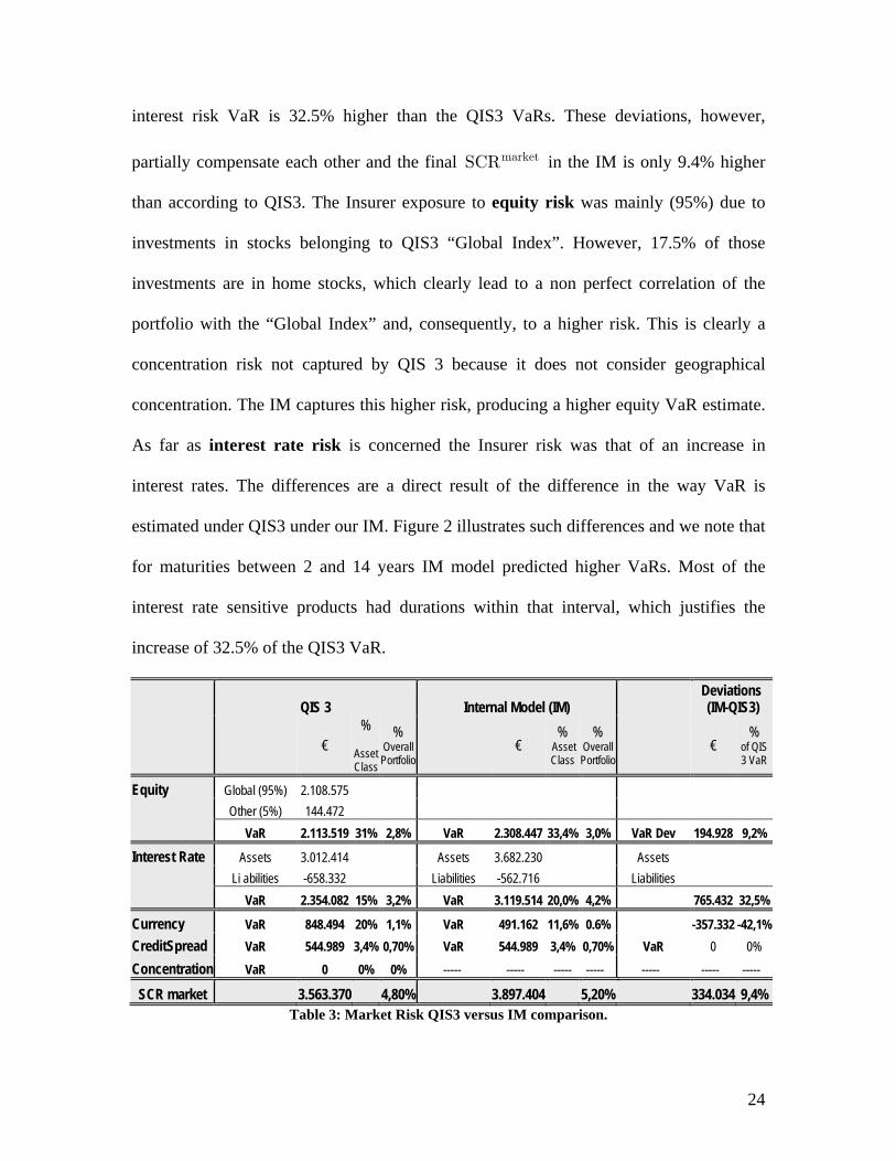
interest risk VaR is 32.5% higher than the QIS3 VaRs. These deviations, however,

partially compensate each other and the final in the IM is only 9.4% higher

than according to QIS3. The Insurer exposure to equity risk was mainly (95%) due to

investments in stocks belonging to QIS3 “Global Index”. However, 17.5% of those

investments are in home stocks, which clearly lead to a non perfect correlation of the

portfolio with the “Global Index” and, consequently, to a higher risk. This is clearly a

concentration risk not captured by QIS 3 because it does not consider geographical

concentration. The IM captures this higher risk, producing a higher equity VaR estimate.

As far as interest rate risk is concerned the Insurer risk was that of an increase in

interest rates. The differences are a direct result of the difference in the way VaR is

estimated under QIS3 under our IM.

marketSCR

Figure 2 illustrates such differences and we note that

for maturities between 2 and 14 years IM model predicted higher VaRs. Most of the

interest rate sensitive products had durations within that interval, which justifies the

increase of 32.5% of the QIS3 VaR.

QIS 3 Internal Model (IM) Deviations (IM-QIS3)

€

%

Asset Class

% Overall Portfolio

€ %

Asset Class

% Overall Portfolio

€ %

of QIS 3 VaR

Equity Global (95%) 2.108.575 Other (5%) 144.472 VaR 2.113.519 31% 2,8% VaR 2.308.447 33,4% 3,0% VaR Dev 194.928 9,2%

Interest Rate Assets 3.012.414 Assets 3.682.230 Assets Li abilities -658.332 Liabilities -562.716 Liabilities VaR 2.354.082 15% 3,2% VaR 3.119.514 20,0% 4,2% 765.432 32,5%

Currency VaR 848.494 20% 1,1% VaR 491.162 11,6% 0.6% -357.332 -42,1% CreditSpread VaR 544.989 3,4% 0,70% VaR 544.989 3,4% 0,70% VaR 0 0% Concentration VaR 0 0% 0% ----- ----- ----- ----- ----- ----- -----

SCR market 3.563.370 4,80% 3.897.404 5,20% 334.034 9,4% Table 3: Market Risk QIS3 versus IM comparison.

24

30,0%

40,0%

50,0%

60,0%

70,0%

80,0%

90,0%

100,0%

1 3 5 7 9 11 13 15 17 19 21 23 25 27

29

QIS3 Internal Model

Figure 2: Comparison of QIS3 and IM VaR for interest rate changes

The Insurer was exposed to currency risk both because of direct investments in foreign

currency and because it had investments in products denominated in foreign currencies.

The exposure was, however, only in the following currencies: GBP (38%), CHF (32%),

SEK (17%) and NOK (13%). The lower VaR produced by the IM can easily be

understood as all these currencies are strong currencies with low variation relative to the

euro. Despite that the QIS3 approach fixed a 20% depreciation to compute the VaR. The

absence of credit spread risk difference results from having adopted, for the IM, the

standard approach proposed in QIS3. In our Insurer case 65.2% of credit sensitive

investment were rated AAA or AA, 30.3% A and the remaining BBB. So, to some

extend, this exposure was too small to justifying the development of an IM alternative.

QIS 3 Equity Interest Rate Currency Credit Spread IM Equity Interest Rate Currency Credit Spread Equity 1 Equity 1 Interest Rate 0 1 Interest Rate -0,033 1 Currency 0,25 0,25 1 Currency -0,064 0,045 1 Credit Spread 0,25 0,25 0,25 1 Credit Spread 0,079 -0,154 -0,007 1

Table 4: QIS3 versus Internal Model estimated correlations between the various market risks.

Table 4 compares the correlations used by the QIS3 and IM for aggregating all market

risk. We note that the QIS3 numbers are not based upon estimations while the IM are.

The QIS3 suggested matrix gives higher correlations than what seems to realistic.

25

3.2 Insurance Risks

Table 6, bellow, presents the results concerning the underwriting risk. To estimate the

premium risk in the IM we have used premium and loss data on 20 Portuguese insurers

during 20 years. Starting values for the parameters were and

. After 4 additional steps we reached the final values of

and The final 20 values for the ‘s can be seen in Vicente

(2008), is the value for the Insurer. From there we got the values for the

mean and variance of

(0)1 0.0539θ =

(0)2 0.0125θ =

(4)1 1.019.543€θ =

14λ =

(4)2 0€θ = iλ

4.2969

2006[ ]EY = 4.297 and 2006[ ] 0V Y = .189 . Concerning reserve risk

there was available a triangle of data from 2001 to 2006 with the occurrence year and the

corresponding claim payment developments, see Table 5.

1 2 3 4 5 6 2001 7.792.345 2.262.154 166.760 393.132 206.338 86.2682002 9.545.760 4.324.696 768.550 613.266 240.614 2003 11.879.234 5.522.645 646.284 571.696 2004 13.804.560 4.993.800 1.230.524 2005 15.336.473 7.390.653 2006 18.170.211

Table 5: Matrix of the incremental paid claims

Because we have insufficient data for the estimation of the correlation coefficients we use

as an estimate the average of the coefficients of the Portuguese insurers in the motor

branch. The standard deviations are calculated with the data of received premiums and

loss reserves. The final results for the premium risk and the reserve risk are shown in

Table 6. More details on the all procedure can be found in Vicente (2008). The main

difference between the QIS3 and IM underwriting risk evaluation is due to the fact that

the IM uses basically information of the Portuguese instead of the European market as the

26

QIS3 does. This application concerns with the motor insurance and is known that

Portuguese drivers have a loss rate greater than the European counterpart, giving support

to using Portuguese data only.

QIS3 IM Deviation Premium Risk PMV 58.610.179 RP 51,549,852

Iσ 49,8% LR 120.03%

Mσ 10,0% ER 25,46% C 0,667 VaR 23,448,828 prσ 41%

Reserve Risk RMV 28.972.444 Mean 14,615,425 resσ 12,5% RES 27,483,984

SE 5,339,722 VaR 12,868,559

Underwriting Risk VM 87.582.623

σ 10,70% ,pr resρ 0.3789 )(f σ 0,3133

underwritingSCR 27.395.091 28.805.711 1.410.620 5,15% Table 6: Underwriting Risk, QIS3 versus IM comparison

On what concerns counterparty risk and operational risk we followed fully the QIS3

directives. Our Insurer had only one reinsurance contract and no financial derivatives. As

the reinsurer had rated “A” by Standard&Poors its estimated probability of default was

considered to be of 0.05%. The replacement cost was of 6,079,915€ and, thus the final

For operational risk, we got the following values for the

pairs (Gross Premiums, Gross Technical Reserves) as (55,660,560, 51,549,852) and

(39,026,522, 51,549,852) respectively for the QIS3 and the Internal Model.

counterpartySCR 303,996€.=

Across all insurance risks the main difference, between the two models are in the way

they handle the underwriting risk. Not surprisingly it is here that we find bigger SCR

discrepancies.

27

3.3 Conclusion

QIS 3 IM Deviations (%) marketSCR 3.563.370 3.897.404 9,40% counterpartySCR 3.03.9.96 303.996 0% underwritingSCR 27.395.091 28.805.711 5,10% basicSCR 28.144.636 29.627.565 5,30% operationalSCR 1.113.211 1.030.997 -7,40%

SCR Final 29.257.847 30.658.562 4,80% Table 7: SCR, QIS3 vs Internal Model

Table 7 summarizes the quantities for the two approaches we worked out for the different

risks. The structures of the two methods are similar allowing for a risk to risk

comparison. On a quick look we find that the capital requirements are quite similar

although the Internal Model gives (slightly) higher requirements. Given a company value,

at the end of 2006, of about 50 million €, the Insurer remain solvent under any of the

proposed approaches. However, we must say that the models used have obvious

limitations. The analysis is not dynamic, for instance it assumes that the business

structure remains the unchanged, no new insurance contracts and the asset structure is the

same. Also, the IM is quite simplified, to ease the calculations and adapt to the

information available, which quite often is limited. Finally, the QIS3 approach is not yet

settled and it is expected soon that a new project, called QIS4, is launched by CEIOPS.

Besides that, there are risks not developed like cat risk, by its complexity (e.g. see the

model by Lescourret and Robert (2006)). Also, as we said earlier, operational risk needs a

better development. The possibility of a derivatives market was not considered here and

could serve as risk mitigation. Also we made the (usual) assumptions concerning

probability distributions fit of some random factors, like the lognormal for the loss ratio,

without enough supporting data.

28

As a final remark we must say that a great step has been taken concerning risk assessment

for insurers, and that the official model proposed by the European control bodies can be

the model built by the insurer herself, although subject to approval. This is in fact

encouraged.

References

Artzner, P., F. Delbaen, J.-M. Eber and D. Heath. “Coherent Measures of Risk”, Mathematical Finance, Vol.9 No.3 (1999), 203-228.

Bühlmann, H. and Gisler, A. (2005) A Course in Credibility Theory and its Applications, Springer.

Comitee of European Insurance and Occupational Pensions Supervisors, “QIS3 – Technical Specifications”, CEIOPS Consultive Document, CEIOPS-FS-11/07 (2007a).

Comitee of European Insurance and Occupational Pensions Supervisors, “QIS3 – Callibration of the underwriting risk and MCR”, CEIOPS Consultive Document, CEIOPS-FS-14/07 (2007b).

Comitee of European Insurance and Occupational Pensions Supervisors, “QIS3 – Callibration of credit risk”, CEIOPS Consultive Document, CEIOPS-FS-23/07 (2007c).

Cont, R. “Empirical properties of asset returns: stylized facts and statistical issues”, Quantitative Finance, Vol.1 No.2 (2001), 223-236.

Dowd, K. (2005). Measuring Market Risk, 2nd Ed., MA:John Wiley & Sons.

El-Bassiouni, M.Y. “A Mixed Model for Loss Ratio Analysis”, ASTIN Bulletin, Vol.21 No.2 (1991), 231-238.

Eling, M., H. Schmeiser and J.T. Schmit “The Solvency II Process: Overview and Critical Analysis”, Risk Management & Insurance Review, Vol.10 N.1 (2007), pp. 69-85

European Commission, “Financial Services: Building a Framework for Action, Communication of the Commission”, Working Paper, 1998-10-28, Brussel 1998.

European Commission, “Design of a Future Prudential Supervisory System in the EU – Recommendations by the Commission Services” Markt/2509/03, Working Paper, Brussels, 2003.

Hesterberg, T., Monaghan, S., Moore, D., Clipson, A. and Epstein, R. (2003), Bootstrap Methods and Permutation Tests, New York: W. H. Freeman and Company.

29

30

Jorion, P. (2001). Value at Risk: The New Benchmark for Managing Financial Risk, 2nd Ed., MA: McGraw-Hill Trade.

KPMG "Study into the Methodologies to Assess the Overall Financial Position of an Insurance Undertaking from the Perspective of Prudential Supervision", Brussels, (2002).

Lescourret, L. and C. Robert “Extreme dependence of multivariate catastrophic losses”, Scandinavian Actuarial Journal, Vol.2006 No.4 (2006), 203-225.

Liebwein, Risk models for capital adequacy: applications in the context of Solvency II and Beyond, The Geneva Papers, Vol.31 No.2 (2006), pp. 528-550.

Linder, U. and V. Ronkainen “Solvency II, Towards a New Insurance Supervisory System in the EU”, Scandinavian Actuarial Journal, Vol.104 No.6 (2004), pp. 462-474.

Linsmeier, T. and Pearson, N. (1996) Risk Measurement: An Introduction to Value at Risk, University of Illinois at Urbana – Champaign.

Lynn Wirch, J. and M.R. Hardy M.R.. “A synthesis of risk measures for capital adequacy”, Insurance Mathematics and Economics, Vol.25 No.11 (1999), pp. 337-347

Lowe, J., “A Practical Guide to measuring reserve variability using: Bootstrapping, operational time and distribution free approach”, Proceedings of the 1994 General Insurance Convention, Institute of Actuaries and Faculty of Actuaries (1994), 157-196.

Mack, T. “Measuring the Variability of Chain Ladder Reserve Estimates”, Casualty Actuarial Society Forum, Vol.1 Spring (1994), 101-182.

McNeil, A., F. Rüdiger and Embrechts Paul (2005). Quantitative Risk Management: Concepts Techniques and Tools, Princenton, MA: Princeton University Press.

Ronkainen, V., L. Koskinen and R. Berglund “Topical modelling issues in Solvency II”, Scandinavian Actuarial Journal, Vol.2007 No.2 (2007), pp. 135 - 146

Sharma, P. “Prudential Supervision of Insurance Undertakings”, report of the conference of the Insurance supervisory services Conference London, 2002.

Taylor, G. (2000) Loss Reserving: An Actuarial Perspective, Kluwer Academic.

Verrall, R.J. Statistical Methods for the Chain Ladder Technique, (1994), 393-446.

Vicente, A.T. (2008) Requisitos de Capital e Solvência II. Uma Aplicação ao Seguro Automóvel, Master Thesis, ISEG, Technical University of Lisbon.

Weil, R., “Macaulay’s Duration: An Appreciation”, Journal of Business, Vol.46 No.4 (1973), pp. 589-92.