TITLE OF THE PAPER (Arial, 14pct, Bold) - Revista Hidraulica · concurenta nu trebuie sa intelegem...
81
No.4/2015
Transcript of TITLE OF THE PAPER (Arial, 14pct, Bold) - Revista Hidraulica · concurenta nu trebuie sa intelegem...

No.4/2015

ISSN 1453 – 7303 “HIDRAULICA” (No. 4/2015) Magazine of Hydraulics, Pneumatics, Tribology, Ecology, Sensorics, Mechatronics
3
CONTENTS
• EDITORIAL: Nu mai este concurenta factor de progres? / Is Competition No Longer a Factor of Progress?
Ph.D. Petrin DRUMEA
5 - 6
• The Calculation of the Pelton and Francis Turbine Hill Chart Using the HydroHillChart Software
Prof. Dorian NEDELCU PhD, St. PhD Eng. Adelina GHICAN (BOSTAN)
7 - 16
• Experimental Model of Pneumatic Tracking System for Photovoltaic Panel Dr. Eng. Ionel Laurentiu ALBOTEANU
17 - 22
• CFD Study on the Distribution of Fertilizer in the Fertigation Plant Lecturer PhD.eng. Petru Marian CÂRLESCU, PhD.Stud.eng. Oana-Raluca CORDUNEANU, Prof. PhD.eng. Ioan ȚENU, PhD.eng. Gheorghe SOVAIALA, PhD.eng. Gabriela MATACHE, Dipl.eng. Sava ANGHEL, PhD.eng. Nicolae TANASESCU
23 - 31
• Wear Properties of Some W/Cu Materials Prepared by Powder Metallurgy PhD. Claudiu NICOLICESCU, PhD. Iulian ŞTEFAN, PhD. Victor Horia NICOARĂ, PhD. Marius Cătălin CRIVEANU
32- 39
• Research on Cam Channels for Zoom Riflescopes Dipl. eng. Dana GRANCIU
40 - 45
• Researches upon Cavitation Erosion Behavior of some Stainless Steels with Different Structures
Lecturer PhD.Eng. Lavinia Madalina MICU, Prof. PhD.Eng. Ilare BORDEASU, Prof. PhD.Eng. Mircea Octavian POPOVICIU, PhD.Eng. Octavian Victor OANCA, PhD. Student Eng. Laura Cornelia SALCIANU, PhD. Student Eng. Cristian GHERA, Lecturer PhD.Eng. Anton IOSIF
46 - 54
• Multiplexed Delay Compensation and Circular Buffer Method for Moving Average Filtering of Signal Acquired from Tactile Sensors in a Mechatronics System for Walking Analysis
PhDc. Eng. Anghel CONSTANTIN, Prof. PhD. Eng. Constantine DAVID
55- 61
• Effects of Turbo Charging of Spark Ignition Engines Aman GUPTA, Sunny NARAYAN
62- 65
• Validation of a Multiple Linear Regression Model Marin RUSĂNESCU, Anca Alexandra PURCĂREA
66- 70
• Using Load Sensing Control Systems to Increase Energy Efficiency of Hydrostatic Transmissions
PhD. Eng. Corneliu CRISTESCU, Lecturer PhD. Eng. Lavinia Madalina MICU, PhD. Eng. Catalin DUMITRESCU, PhD. Student Eng. Petrica KREVEY
71 - 77
• Experimental Stand for Diagnosis of Mechano-Hydraulic Continuous Variable Transmission
PhD. Student Eng. Nicolae Florin ROTARU, Prof. Liviu Ioan VAIDA, PhD.
78 -81

ISSN 1453 – 7303 “HIDRAULICA” (No. 4/2015) Magazine of Hydraulics, Pneumatics, Tribology, Ecology, Sensorics, Mechatronics
4
BOARD
DIRECTOR OF PUBLICATION
- PhD. Eng. Petrin DRUMEA - Hydraulics and Pneumatics Research Institute in Bucharest, Romania
EDITOR-IN-CHIEF
- PhD.Eng. Gabriela MATACHE - Hydraulics and Pneumatics Research Institute in Bucharest, Romania
EXECUTIVE EDITOR
- Ana-Maria POPESCU - Hydraulics and Pneumatics Research Institute in Bucharest, Romania
EDITORIAL BOARD
PhD.Eng. Gabriela MATACHE - Hydraulics and Pneumatics Research Institute in Bucharest, Romania
Assoc. Prof. Adolfo SENATORE, PhD. – University of Salerno, Italy
PhD.Eng. Catalin DUMITRESCU - Hydraulics and Pneumatics Research Institute in Bucharest, Romania
Assoc. Prof. Constantin CHIRITA, PhD. – “Gheorghe Asachi” Technical University of Iasi, Romania
PhD.Eng. Radu Iulian RADOI - Hydraulics and Pneumatics Research Institute in Bucharest, Romania
Assoc. Prof. Constantin RANEA, PhD. – University Politehnica of Bucharest; National Authority for Scientific Research
and Innovation (ANCSI), Romania
Prof. Aurelian FATU, PhD. – Institute Pprime – University of Poitiers, France
PhD.Eng. Małgorzata MALEC – KOMAG Institute of Mining Technology in Gliwice, Poland
Lect. Ioan-Lucian MARCU, PhD. – Technical University of Cluj-Napoca, Romania
Prof. Mihai AVRAM, PhD. – University Politehnica of Bucharest, Romania
COMMITTEE OF REVIEWERS
PhD.Eng. Corneliu CRISTESCU – Hydraulics and Pneumatics Research Institute in Bucharest, Romania
Assoc. Prof. Pavel MACH, PhD. – Czech Technical University in Prague, Czech Republic
Prof. Ilare BORDEASU, PhD. – Politehnica University of Timisoara, Romania
Prof. Valeriu DULGHERU, PhD. – Technical University of Moldova, Chisinau, Republic of Moldova
Assist. Prof. Krzysztof KĘDZIA, PhD. – Wroclaw University of Technology, Poland
Assoc. Prof. Andrei DRUMEA, PhD. – University Politehnica of Bucharest, Romania
PhD.Eng. Marian BLEJAN - Hydraulics and Pneumatics Research Institute in Bucharest, Romania
Prof. Dan OPRUTA, PhD. – Technical University of Cluj-Napoca, Romania
Ph.D. Amir ROSTAMI – Georgia Institute of Technology, USA
Prof. Adrian CIOCANEA, PhD. – University Politehnica of Bucharest, Romania
Prof. Carmen-Anca SAFTA, PhD. - University Politehnica of Bucharest, Romania
Prof. Ion PIRNA, PhD. – The National Institute of Research and Development for Machines and Installations Designed to
Agriculture and Food Industry - INMA Bucharest, Romania Published by: Hydraulics and Pneumatics Research Institute, Bucharest-Romania Address: 14 Cuţitul de Argint, district 4, Bucharest, 040558, Romania Phone: +40 21 336 39 91; Fax:+40 21 337 30 40; e-Mail: [email protected]; Web: www.ihp.ro with support from: National Professional Association of Hydraulics and Pneumatics in Romania - FLUIDAS e-Mail: [email protected]; Web: www.fluidas.ro HIDRAULICA Magazine is indexed by international databases:
ISSN 1453 – 7303; ISSN – L 1453 – 7303

ISSN 1453 – 7303 “HIDRAULICA” (No. 4/2015) Magazine of Hydraulics, Pneumatics, Tribology, Ecology, Sensorics, Mechatronics
5
EDITORIAL Nu mai este concurenta factor de progres?
De cand am inceput sa fiu interesat de dezvoltarea tehnicii si tehnologiei am fost invatat ca nu poate exista progres tehnic fara concurenta. A fost nevoie de multi ani pentru a intelege ca nu orice fel de lupta este o concurenta generatoare de progres.
Primul care m-a pus pe ganduri a fost un prieten dintr-o tara dezvoltata care mi-a povestit cum ca el are un exemplu destul de interesant. In tara lui existau cateva companii (din cate imi amintesc doua sau trei) de telefonie mobila (sau poate altceva la moda)
Dr. ing. Petrin DRUMEA DIRECTOR DE PUBLICATIE
care se aflau in primele randuri ale domeniului, la nivel european, prin ofertele de inalt nivel tehnic si destul de acceptabile economic. Data fiind dezvoltarea cererii, a aparut in tara respectiva inca o firma (poate chiar doua) care pentru a castiga piata a redus preturile la serviciile oferite. Vechile firme au fost obligate sa reduca si ele preturile pentru a ramane in piata. Reducerea preturilor s-a facut pe seama reducerii calitatii serviciilor, astfel incat in doi ani lucrurile au progresat tehnic foarte putin, iar oamenii au constatat ca nu toate lucrurile merg bine in relatia cu aceste firme. Sigur ca lucrurile s-au redresat in timp (cativa ani), calitatea serviciilor a revenit la un nivel inalt, iar lumea a fost din nou multumita.
Am tratat spusele prietenului din strainatate ca pe o poveste interesanta si nimic mai mult, pana cand am aflat tot de la un prieten, dar de data aceasta din tara, ca la o universitate, destul de importanta, exista doua (sau trei?) departamente care au ca preocupare domeniile mecanica si actionarile hidraulice. Concurenta dintre aceste departamente nu a condus la mai multe laboratoare de inalta tinuta, ci la niste laboratoare formale si de scazut nivel tehnico-stiintific, nu a crescut numarul de brevete de inventii si nici de articole stiintifice de inalt nivel, intrucat nici unii si nici altii nu aveau fonduri suficiente si nici un numar convenabil de specialisti adevarati.
Poate ar fi de interes si situatia de concurenta formala intre specialistii, unii chiar profesori din diversele domenii, care se lupta pe glorie nu prin rezultate stiintifice sau tehnice deosebite, ci prin vorbe, comportament si/sau functii, in asa fel incat in final nu apare in niciun fel factorul de progres.
Mai am cateva exemple de acest fel extinse la toate domeniile si care m-au pus pe ganduri. Oare nu e adevarat ce stie toata lumea cum ca pentru a progresa e nevoie de concurenta? Eu cred ca este adevarata ideea progresului prin concurenta, insa trebuie facuta precizarea ca prin concurenta nu trebuie sa intelegem lupta pentru bani, putere sau avantaje prin metode incorecte, abuzive, neeconomice si neloiale, ci acestea sa rezulte in urma unei dezvoltari serioase, corecte si sustenabile.

ISSN 1453 – 7303 “HIDRAULICA” (No. 4/2015) Magazine of Hydraulics, Pneumatics, Tribology, Ecology, Sensorics, Mechatronics
6
EDITORIAL Is Competition No Longer a Factor of Progress?
Ever since I started to be interested in the development of techniques and technology I was taught that there can be no technical progress without competition. It took many years for me to understand that not just any fighting is competition which generates progress.
The first one who got me thinking was a friend from a more economically developed country who told me that he has a rather interesting example. In his country there were a few (as I recall two or three) mobile phone (or something else popular) companies
Ph.D.Eng. Petrin DRUMEA DIRECTOR OF PUBLICATION
which were in the forefront of the field at European level, by their high technical level and economically quite acceptable market offerings. Given the increasing development in demand, there emerged in that country another company (possibly two of them) which in order to gain market share cut prices for the services provided. The old companies were forced to reduce in turn their prices in order to remain in market. Cutting down prices was made at the expense of service quality, so that in two years things have progressed very little from the technical point of view, and people have found that not all things were going well in the relationship with these companies. Of course, things have recovered with time (in a few years), quality of services went back to a high level, and people were again satisfied.
I took the words of my friend from abroad as an interesting story and nothing more, until I found out, also from a friend, this time from our country, that in an important enough university there were two (or three?) departments dealing with the areas of Mechanics and Fluid Power. Competition between these departments has not resulted in more high quality laboratories but in some formal and low technical and scientific level laboratories, it has not resulted in an increased number of patents or high level scientific papers, as none of them had neither adequate funding nor a fair number of real specialists.
It might also be of interest the case of formal competition between specialists, some of them even professors in various areas, who compete for glory not through outstanding scientific or technological results but through speech, behavior and / or positions, so that in the end there is no way for the factor of progress to arise.
I have some more examples of this kind, extended to all areas, which got me thinking. Isn’t it true what everyone knows, namely that to make progress we need competition? I believe that the idea of progress through competition is true, but it must be made clear that by competition we should not understand the struggle for money, power or benefits by unfair, abusive, uneconomical and dirty means, but all mentioned above should arise from serious, fair and sustainable development.

ISSN 1453 – 7303 “HIDRAULICA” (No. 4/2015) Magazine of Hydraulics, Pneumatics, Tribology, Ecology, Sensorics, Mechatronics
7
The Calculation of the Pelton and Francis Turbine Hill Chart Using the HydroHillChart Software
Prof. Dorian NEDELCU PhD1, St. PhD Eng. Adelina GHICAN (BOSTAN)1
1 “Eftimie Murgu” University of Reşiţa, Romania, [email protected]
Abstract: The paper presents the HydroHillChart software, which is designed to calculate the hill chart for hydraulic turbines (Pelton, Francis and Kaplan) and the operation diagram, based on the energetic primary data that is obtained through turbine model measurements performed on the test rig. The HydroHillChart software is made up of the following four modules: the Pelton, Francis and Kaplan modules – which are used to calculate the turbine model hill chart and the DEX module – which is used to calculate the operation diagram for the industrial turbine prototype. The results of the software consist of graphical curves and numerical results which can be viewed in HydroHillChart and exported as Excel files with a template structure and also as PDF and Word files. The lack of paper space will limit the presentation to the Pelton and Francis modules only.
Keywords: model, turbine, Pelton, Francis, Kaplan, hill chart, software, Python
1. Introduction
The design of hydraulic turbines is based on energetic and cavitation characteristics, obtained by measuring the turbine models in the test rig. The efficiency hill chart can be obtained through graphical packages, like general graphic processing and by computer-aided design programs, or through specialized programs like [1]. The HydroHillChart software was created using Python – a high-level object-oriented language and related modules: wxPython - a graphical user interface toolkit for the Python language, matplotlib - a python 2D plotting library which produces publication quality figures, SQLite – a database engine, SciPy - a Python-based ecosystem of open-source softwares for mathematics, science, and engineering. The HydroHillChart software, presented at http://www.cchapt.ro/HydroHillChart.htm, is a continuation of the Preldate software, which was originally conceived to compute the characteristics of hydraulic turbines [2], [3] and is the result of a PhD thesis [4], using tools similar with those from [5]. 2. The HydroHillChart main interface
The HydroHillChart software is equipped with instruments for zooming (fit, pan, zoom in, zoom out), for spline curves interpolations, for graph intersections with constant X or Y values, for saving the graph as an image file and for the modification of the general/graph setting. For each graph generated by the HydroHillChart software, a toolbar with command buttons that are marked with specific icons appears at the bottom of the window. It performs the following functions:
Home - Return to initial view;
Pan - Left click & hold to zoom,
zoom in/out with the right mouse button pressed;
Back - Back to previous view;
Forward - Forward to the next view;
Save - Save chart format: EPS;
JPG, PGF, PDF; PNG, PS; RAW, SVG, TIF;
Zoom - Enlarge selected area; Subplots - Chart configuration.
Fig. 1 shows the main menu of the HydroHillChart software. From the “File” menu, one can select the type of turbine for which the hill chart will be calculated (Pelton, Francis or Kaplan turbine) or the DEX option for which the operation diagram can be calculated. Based on the measured data of the turbine model, the software generates the hill chart for turbine models and the operation diagram for the industrial turbine prototype, providing the necessary tools for designing a turbine:

ISSN 1453 – 7303 “HIDRAULICA” (No. 4/2015) Magazine of Hydraulics, Pneumatics, Tribology, Ecology, Sensorics, Mechatronics
8
graphic visualization of functional dependencies, intersections in the hill chart and in the operation diagram, the generation of numerical results and their export in the usual programs: Excel, Word, PDF. The 2D curve interpolations are calculated by using the cubic spline functions. The constant efficiency curves are numerically and graphically generated using the mplot3d toolkit, which is included in the matplotlib library [6].
Fig. 1. The HydroHillChart main menu
3. HydroHillChart – Pelton module
The Pelton module [7], [8] can be selected from the “Pelton Turbine” option of the main menu and it displays a window with a specific interface, Fig. 2, composed of: a toolbar, a measured data table, called “Measured Points”, which stores measured data for a model runner and a table called “Intersection with efficiency constant values”, where the application stores values arising from the intersection of primary curves with constant efficiency values.
Fig. 2. The HydroHillChart interface for the Pelton module
The primary data is taken from Excel and stored in the table called “Puncte măsurate - Measured Points” by completing the following fields:
• ID Point - represents the current number for the measured point; • S [mm] - represents the nozzle spear opening of a Pelton model; • Q11 [m
3/s] - represents the unit discharge; • n11 [rot/min] - represents the unit speed; • η [%] - represents the efficiency;

ISSN 1453 – 7303 “HIDRAULICA” (No. 4/2015) Magazine of Hydraulics, Pneumatics, Tribology, Ecology, Sensorics, Mechatronics
9
• Eliminated point – allows the removal of a measured point, by selecting a Check Box control.
The Pelton module toolbar is located at the top of the window and includes control buttons marked with specific icons, figure 2, which fulfill the following functions:
- informative icon for the Pelton runner, without a related function;
New
- create a new database for Pelton runners;
Open
- open and load an existing database for Pelton runners;
Info
- provides information about the current database;
Data
- primary data visualization in graphic form: 3D curves and ),,( SQnf=1111
η 3D
surface, respectively 2D curves at S parameter and S = f (Q11); )(
11nf=η
,(11
Qnf=η ( )11
Qf=η ( )Sf=η
),( 1111 Qnf=η
),( Qnf=η
),(1111
Qnf=η
Hill Chart
- calculating and plotting of the hill chart for a number of specified efficiencies values;
n11
- imposing a double unit speed n11 to calculate the characteristics’ intersection
in order to determine the curve respectively ; )11
Q11-n11
- imposing a double unit speed n11 and unit discharge Q11, followed by a hill chart
intersection in order to calculate the efficiency point (Q11, n11);
Excel
- export results in an Excel file: input data and the numerical and graphical processing carried out;
Word
- graphics export in a Word file;
- graphics export in a PDF file;
Exit
- return to the main window of the HydroHillChart software.
The HydroHillChart - Pelton module software will be verified through calculation and a hill chart comparison for the following Pelton models which was taken from literature:
• K560 runner with a diameter D = 375 mm, 24 buckets and 6 nozzle spears with a diameter of Ø42mm; the primary data was taken from measurements performed on the [11] model, page 98; from the hill chart of Fig. 3, a matrix point was extracted for the following nozzle spear openings S=5, 10, 15, 20, 25, 30, 40 mm and imported as primary data to the HydroHillChart – Pelton module software;
• K600/461 runner with a diameter D = 450 mm, 20 buckets and 6 nozzle spears with Ø47.25 mm in diameter [12], page 31; from the hill chart of Fig. 4, a matrix point was extracted for the following nozzle spear openings S=7.5, 10, 12.5, 15, 20, 40 mm and imported as primary data to the HydroHillChart – Pelton module software;
Fig. 5, 6 and 7 show the 3D surface, the 3D intersection curves with constant efficiency values and the hill chart for the Pelton K560 runner, generated by the HydroHillChart –Pelton module software. Fig. 11 shows the HydroHillChart comparison for the Pelton K560 runner.
1111
Fig. 8, 9 and 10 show the 3D surface, the 3D intersection curves with constant efficiency values and the hill chart for the Pelton K600/461 runner, generated by the HydroHillChart – Pelton module software. Fig. 12 shows the HydroHillChart comparison for the Pelton K600/461 runner.

ISSN 1453 – 7303 “HIDRAULICA” (No. 4/2015)
10
Magazine of Hydraulics, Pneumatics, Tribology, Ecology, Sensorics, Mechatronics
Fig. 3. The hill chart for the Pelton K560 runner and the matrix points
Fig. 4. The hill chart for the Pelton K600/461 runner and the matrix points
Fig. 5. The 3D surface ),(1111
Qnf=η
for the Pelton K560 runner
Fig. 6. The 3D intersection curves with constant
efficiency values for the Pelton K560 runner
Fig. 7. The 2D hill chart for the Pelton K560 runner calculated by using HydroHillChart

ISSN 1453 – 7303 “HIDRAULICA” (No. 4/2015) of Hydraulics, Pneumatics, Tribology, Ecology, Sensorics,
11
Magazine Mechatronics
Fig. 8. The ),(1111
Qnf=η 3D surface Fig. 9. The 3D intersection curves with constant
Fig. 11. The 2D hill chart comparison for the Pelton K560 runner
For the P runner elton K600/461efficiency values for the Pelton K600/461 runner
Fig. 10. The 2D hill chart for the Pelton K600/461 runner calculated by using HydroHillChart

ISSN 1453 – 7303 “HIDRAULICA” (No. 4/2015)
12
Magazine of Hydraulics, Pneumatics, Tribology, Ecology, Sensorics, Mechatronics
Fig. 12. The 2D hill chart comparison for the Pelton K600/461 runner
. HydroHillChart – Fra
lected from the “Francis Turbine” option of the main menu
Fig. 13. The HydroHillChart interface for the Francis module
The Francis module des control buttons
4 ncis module
The Francis module [9], [10] can be seand it displays a window with a specific interface, Fig. 13, composed of: a toolbar, a measured data table, called “Measured Points”, which stores measured data for a model runner and a table called “Intersection with efficiency constant values”, where the application stores values arising from the intersection of primary curves with constant efficiency values.
toolbar is located at the top of the window and inclumarked with specific icons, which fulfill functions similar to those of the Pelton module. The primary data is similar to the Pelton module, with the exception of ao [mm], which represents the wicked gate opening and replaces the S parameter. For a Francis turbine model, measurements can be performed by using the following parameters ao=const., wicked gate opening, or n11=const., unit speed. Although the input data fields are identical, for all measurement scenarios, graphic representation and calculation algorithms differ for the two scenarios. The resulting curves are

ISSN 1453 – 7303 “HIDRAULICA” (No. 4/2015) Magazine of Hydraulics, Pneumatics, Tribology, Ecology, Sensorics, Mechatronics
13
different, but if the interpolations are precise enough, the hill chart should coincide. Thereby, for a data set where the matrix point (n11, Q11, ao, η) is at the intersection of a ao=const. range of values with a n11=const. range of values, the hill chart, which arises from the primary data considered to be measured at ao=const., should overlap with the one which arises from the primary data considered to be measured at n11=const. An example of the comparison is presented in Fig. 14. As shown in the figure, the difference between the isolines is insignificant and that validates the interpolation algorithms used to calculate the hill chart with the HydroHillChart software.
Fig. 14. The 2D hill chart comparison for ao / n11=const. scenarios
The HydroHillChart and a hill chart
he primary data was
ith a diameter D = 460 mm and 13 runner blades; the primary data was
Fig. 15. The hill chart for the Francis F316.5 runner Fig. 16. The hill chart for the Francis RO 115
- Francis module software will be verified through calculation comparison for the following Francis models which was taken from literature:
• F316.5 runner with a diameter D = 460 mm and 14 runner blades; ttaken from measurements performed on the [13] model, page 68; from the hill chart of Fig. 15, a matrix point was extracted for the following wicked gate openings: ao=14, 18, 22, 26, 30, 34, 38, 42, 46, 50 mm and imported as primary data to the HydroHillChart – Francis module software;
• RO 115 runner wtaken from measurements performed on the [12] model, page 69; from the hill chart of Fig. 16, a matrix point was extracted for the following wicked gate openings : ao=14, 18, 22, 26, 30, 34, 38, 42 mm and imported as primary data to the HydroHillChart – Francis module software;
and the matrix points runner and the matrix points

ISSN 1453 – 7303 “HIDRAULICA” (No. 4/2015) Magazine of Hydraulics, Pneumatics, Tribology, Ecology, Sensorics, Mechatronics
14
Fig. 17, 18 and 19 show the 3D surface, the 3D intersection curves with constant efficiency values and the hill chart for the Francis F316.5 runner, generated by the HydroHillChart –Francis module software. Fig. 23 shows the HydroHillChart comparison for the Francis F316.5 runner.
),(1111
Qnf=η
),(1111
Qnf=η
Fig. 18. The 3
),(1111
Qnf=
Fig. 20, 21 and 22 show the 3D surface, the 3D intersection curves with constant efficiency values and the hill chart for the Francis RO 115 runner, generated by the HydroHillChart –Francis module software. Fig. 24 shows the HydroHillChart comparison for the Francis RO 115 runner.
Fig. 17. The 3D surface ),(1111
Qnf=η
For the Francis F316.5 runner
D intersection curves with constant
es for the Francis F316.5 runner efficiency valu
Fig. 19. The 2D hill chart for the Francis F316.5 runner calculated by using HydroHillChart
Fig. 20. The η 3D surface
for the Francis RO 115 runner
Fig. 21. The 3
efficiency valu
D intersection curves with constant
es for the Francis RO 115 runner

ISSN 1453 – 7303 “HIDRAULICA” (No. 4/2015) of Hydraulics, Pneumatics, Tribology, Ecology, Sensorics,
15
Magazine Mechatronics
r the Francis RO 115 runner
Fig. 22. The 2D hill chart for the Francis RO 115 runner calculated by using HydroHillChart
Fig. 23. The 2D hill chart comparison for the Francis F316.5 runner
Fig. 24. The 2D hill chart comparison fo

ISSN 1453 – 7303 “HIDRAULICA” (No. 4/2015) Magazine of Hydraulics, Pneumatics, Tribology, Ecology, Sensorics, Mechatronics
16
5. Conclusions
Small differences between the original efficiency curves which were taken from literature and the HydroHillChart calculated curves can be observed in Fig. 11, Fig. 12, Fig. 23, Fig. 24, but the shapes are similar and the curves overlap on their longest length. Those hill charts were calculated by using different mathematical interpolation tools and by starting from different primary data: the original efficiency curves taken from literature were calculated by starting from the points that were measured on the turbine model; the HydroHillChart curves were calculated by starting from the matrix points that were extracted from the literature hill chart, Fig. 3, Fig. 4, Fig. 15, Fig. 16, which also lead to these differences. The differences can be reduced by increasing the number of matrix points extracted from the literature hill chart. HydroHillChart is a powerful software, equipped with all the necessary instruments to calculate, generate and explore the hill chart, based on the turbine model measurements, offering 2D/3D graphical and numerical results. The comparison of characteristics that were taken from literature with those calculated using the HydroHillChart software confirms the correctness of the interpolation algorithms that were used. In the future, the software will focus on the characteristics of the cavitation turbines [14].
Acknowledgements
The work has been funded by the Sectoral Operational Programme Human Resources Development 2007-2013 of the Ministry of European Funds through the Financial Agreement POSDRU/159/1.5/S/132395.
References
[1] G. A. Aggidis*, A. Zidonis, “Hydro turbine prototype testing and generation of performance curves: Fully automated approach”, Renewable Energy, 71, 2014, pp 433-441;
[2] D. Nedelcu, C.V. Campian, “Software for Computing of the Hydraulic Turbines Characteristics”, The 6th International Conference on Hydraulic Machinery and Hydrodynamics, Timisoara, Romania, October 21 - 22, 2004, pp 137-142;
[3] D. Nedelcu, “Numerical Methodology for Computing the Hydraulic Turbine Hill Chart“, Proceedings of the Workshop on Numerical Methods in Fluid Mechanics and Fluent Applications, Timişoara, May 22-23, 2003, pp. 179-186;
[4] A. Ghican (Bostan),”Contributions regarding the improving of experimental measurement methods and processing the results on the test rig for hydraulic turbine models”, PhD Thesis, PhD Supervisor Prof. D. Nedelcu, “Eftimie Murgu” University of Reşiţa, 2015;
[5] D. Nedelcu, “Voice commands of a 2D graph“, SISOM 2010 and Session of the Commission of Acoustics, Bucharest, May 27-28, 2010;
[6] J. D. Hunter, “Matplotlib. A 2D graphics environment”, Computing In Science & Engineering, Vol. 9, No. 3, pp. 90-954, Publisher IEEE COMPUTER SOC., 2007.
[7] D. Nedelcu, A. Ghican (Bostan), F. Periş-Bendu, “HydroHillChart - Pelton module. Software for calculating universal characteristic of Pelton hydraulic turbines“, “Eftimie Murgu” University Annals, Year XXI, No. 1, ISSN 1453 - 7397, Reşiţa, 2015;
[8] A. Ghican (Bostan), D., Nedelcu, F. Periş-Bendu, “Calculation of universal characteristics for Pelton runner models using the HydroHillChart - Pelton module software“,“Eftimie Murgu” University Annals”, Year XXI, No. 1, ISSN 1453 - 7397, Reşiţa, 2015;
[9] D., Nedelcu, A. Ghican (Bostan), F. Periş-Bendu, “HydroHillChart – Francis module. Software for calculating universal characteristic of Francis hydraulic turbines“,“Eftimie Murgu” University Annals, Year XXI, No. 1, ISSN 1453 - 7397, Reşiţa, 2015;
[10] A. Ghican (Bostan), D., Nedelcu, F. Periş-Bendu, “Calculation of universal characteristics for Francis runner models using the HydroHillChart - Francis module software“Eftimie Murgu” University Annals, Year XXI, No. 1, ISSN 1453 - 7397, Reşiţa, 2015;
[11] Iu.U. Edel, “Turbine hidraulice Pelton. Teorie, cercetare, calcule” (Russian translation), Masghiz Publisher, Moscova, 1963;
[12] N. N. Kovalev, “Turbine hidraulice. Construcții și probleme de proiectare”, (Russian translation), Mașinostroienie Publisher, Leningrad, 1971;
[13] D.S. Shavelev, “Echipament hidroenergetic și auxiliar de la centralele hidroelectrice”, (Russian translation), Vol. 1, Energoizdat Publisher, Moscova, 1988;
[14] I. Bordeiaşu, M.O. Popoviciu, “Cavitation erosion resistance for a set of stainless steels having 10% Nickel and variable Chromium concentrations”, Revista Hidraulica, no. 1/ 2013, pp. 79-85.

ISSN 1453 – 7303 “HIDRAULICA” (No. 4/2015) Magazine of Hydraulics, Pneumatics, Tribology, Ecology, Sensorics, Mechatronics
17
Experimental Model of Pneumatic Tracking System for Photovoltaic Panel
Dr. Eng. Ionel Laurentiu ALBOTEANU1
1 University of Craiova, Faculty of Electrical Engineering, [email protected]
Abstract: Because conventional energy production resources are limited, mankind headed for using other sources of energy, alternative, inexhaustible. Solar energy is an alternative to traditional sources. However, the conversion of solar energy into electricity using photovoltaic effect is achieved with low yield (15-18% when using monocrystalline silicon). A method for increasing the yield is based on the use of tracking systems for photovoltaic panels. The paper aims to experimentally validate the theory presented in the paper ˝Pneumatic Tracking System for Photovoltaic Panel˝ [2].
Keywords: pneumatic drive, tracking system, photovoltaic (PV) panel, programmable logic controller (PLC)
1. Introduction
To increase photovoltaic yield and electricity production photovoltaic tracking systems are sometimes used. The photovoltaic tracking system is a device capable of turning after the Sun, which means following the Sun’s track from its rising in the east to its setting in the west. The photovoltaic tracking system is a mechanical construction and the photovoltaic panels are attached to this construction. Because the tracking system turns after the Sun all day long, the solar panels are set to face the Sun directly all day long, and so is their performance substantially enhanced. This process allows the energy usually generated using static photovoltaic panels to be increased by as much as 45% [19]. Optimal alignment is made possible by a precise astronomical control mechanism which can plot the course of the sun from any geographical location at a given time of the year. The most of photovoltaic tracking systems uses the electric drive. In the paper ˝Pneumatic Tracking System for Photovoltaic Panel˝ [2] is shown another type of tracking system based on a pneumatic drive. Of the existing tracking systems in literature [8], the pseudo-equatorial system was adopted. This tracking system was particularized for Craiova location.
2. Structure of mechanical part of tracking system
The tracking systems contain controlled mechanisms that allow maximization of direct normal radiation received on PV panel [9]. As specified in [2], a pseudo-equatorial tracking system type has been adopted for reason of savings in terms of energy efficiency and material consumption. Pneumatic drive was chosen due to the following advantages [2], [10], [17]: - their structures are simple and suited for mass production; - the forces, moments and engine speeds can be adjusted easily using simple devices; - pneumatic motor overload does not introduce risk of damage; - pneumatic transmissions allow starts, stops, frequent and sudden changes of direction without risk of damage; - compressed air is relatively easy to produce and transport network is environmentally friendly non-flammable; - can be stored in high quantity; - risk of injury is reduced; - easy maintenance. The structure of the mechanical part of a tracking system is shown in Figure 1. As shown in the figure, a single pneumatic cylinder was used for orientation of a photovoltaic panel after E-W (azimuth) axis. For S-N axis (elevation) a screw-nut mechanism of orientation was used. According to schematic diagram in Figure 1, it was started the effective realization of an experimental tracking system. The experimental model achieved is shown in Figure 2.

ISSN 1453 – 7303 “HIDRAULICA” (No. 4/2015) Magazine Mechatronics
18
of Hydraulics, Pneumatics, Tribology, Ecology, Sensorics,
Fig. 1. Structure of the mechanical part of a tracking system : 1- photovoltaic (PV) panel; 2- mechanical
mount of PV panel; 3- azimuth tracking mechanism (E-W direction); 4- azimuth joint motion; 5- pneumatic cylinder; 6- elevation joint motion (S-N direction); 7- elevation tracking mechanism; 8- support tower
Fig. 2. Experimental model of tracking system: 1- PV panel; 2- mechanical mount of PV panel; 3- azimuth
tracking mechanism; 4- azimuth joint motion; 5- pneumatic cylinder; 6- elevation tracking mechanism; 7- throttles; 8- position sensors; 9- electrical equipment for power supply and control;10- support tower

ISSN 1453 – 7303 “HIDRAULICA” (No. 4/2015) Magazine of Hydraulics, Pneumatics, Tribology, Ecology, Sensorics, Mechatronics
19
3. Structure of power supply and control part of tracking system
After achieving the mechanical part of tracking system there has been made the power supply and automatic control part. The orientation of PV panel will be made automatically according to astronomical data using a PLC. For reasons of optimization in terms of economic efficiency, PV panel will perform a movement in steps, with three stationary positions over the day. The experimental model finished is shown in Figure 3.
Fig. 3. Experimental model of tracking system – electrical part:
1- equipment for production and preparation of compressed air (compressor, air storage accumulator, filter, pressure regulator, decanter, pressure gauge); 2- DC power supply 24V; 3- terminal strip; 4- programmable
logic controller (PLC) Easy Moeller; 5- solenoid valve (electrically controlled distributor); 6- Start-Stop switch; 7- mechanical part of tracking system.
For automatic orientation of the photovoltaic panel a PLC from Moeller family, namely Easy 512 DC-RC, was chosen due to its advantages over other control equipment [21]. Figure 4 presents the wiring diagram of the tracking system. It contains the following equipment: PLC; two power supplies (one for input circuits of the PLC and the other for output circuits); X and Y coils of valve; Start / Stop buttons for power supply; L1, L2, L3 - position sensors; BP- button of work program initialization. Figure 5 shows how to achieve electrical wiring and pneumatic ways with elements related to pneumatic actuation. One can notice the two DR1 and DR2 throttles path having the role of regulating the speed of pneumatic cylinder rod.

ISSN 1453 – 7303 “HIDRAULICA” (No. 4/2015)
20
Magazine of Hydraulics, Pneumatics, Tribology, Ecology, Sensorics, Mechatronics
Fig. 4. Wiring diagram of the pneumatic tracking system
Fig. 5. Diagram of Easy Moeller PLC connecting to the pneumatic actuation

ISSN 1453 – 7303 “HIDRAULICA” (No. 4/2015) Magazine of Hydraulics, Pneumatics, Tribology, Ecology, Sensorics, Mechatronics
21
For the development of the photovoltaic panel orientation program there has been used the dedicated software for family Easy Moeller PLC, called Easy Soft [21]. The program may be made easier if initially there is developed the flow chart based on logic functions "Function Block". In Figure 6 is shown the program window made by way of diagram of connections.
Fig. 6. Window program for tracking system of PV panel
The notations in the figure have the following meanings: I01- PLC input 1- Button Start/Stop program; I02, I03, I04 – PLC 2,3,4 inputs, corresponding to the three position sensors; T01, T02, T03 – timings; M01...M04 – markers (memory elements of the command - latching); Q1, Q2 – PLC outputs 1 and 2 of PLC corresponding to the power supply of the two coils of valves. For activation of inputs I01, the coil of M01 marker is supplied, which will feed 3 timers (T01, T02, T03), through the switch M01. The three relays will be adjusted so timings: T01=4hours; T02=8 hours; T03=12 hours. So during the day the photovoltaic panel is moved 3 times (will have 3 positions). Timing T01 will start at 8:00 AM and upon passing of 4 hours the switch T01 will close and Q01 output will be activated. The PV panel is moved up to touch sensor corresponding to I03 input latching marker M03. 8 hours after the time given by T02, the panel is moved again up to touch of the sensor corresponding to I02 input, latching of marker M02. After 12 hours of delay time given by T03, the panel will be brought to its original position by T03 contact closure which will enable the Q03 output of PLC, which will power supply the other coil of the distributor. Stopping of the PV panel will be given by the sensor corresponding to I04 input. The command will be maintained by M04 marker. Stopping of the running program will be done by disabling input I01.

ISSN 1453 – 7303 “HIDRAULICA” (No. 4/2015) Magazine of Hydraulics, Pneumatics, Tribology, Ecology, Sensorics, Mechatronics
22
Conclusions
In this work are presented practical aspects regarding the implementation of a tracking system for photovoltaic panels based on a pneumatic drive. The elements relating to practice have been made based on theoretical solutions proposed in the paper [2]. Both the mechanical part of developed tracking system as well as power supply and command part have been proven correct functioning according to the solution and protocol required in [2].
References
[1] I. L. Alboteanu, ˝Advanced stand-alone photovoltaic system˝, Universitaria Publishing House, Craiova, 2013;
[2] I. L. Alboteanu, ˝Pneumatic Tracking System for Photovoltaic Panel˝, ˝ Hidraulica˝, No. 1/2015, ISSN 145-7303, pp. 32-39;
[3] I. L. Alboteanu, F. Ravigan, and A. Novac, ˝Automation of a Sun Tracking System for Photovoltaic Panel with Low Concentration of Solar Radiation˝, ˝Annals of the University of Craiova: Engineering series˝, No38/2014, ISBN 1842-4805, pp. 157-163;
[4] I. L. Alboteanu, F. Ravigan, and S. Degeratu, ˝Methods for Increasing Energy Efficiency of Photovoltaic Systems˝, ˝International Journal of Power and Renewable Energy Systems˝, No.1/2014, ISBN: 2374-376X, pp. 51-61;
[5] I. L. Alboteanu, Gh. Manolea, F. Ravigan, and A. Nour, ˝Strategy of Control for Solar Panels Positioning Systems˝, ˝Annals of the University of Petrosani, Electrical Engineering˝, vol. 9, 2007, ISSN: 1343-8418, pp. 347-363;
[6] I. L. Alboteanu, F. Ravigan, S. Degeratu, C. Sulea, “Aspects of designing the tracking systems for photovoltaic panels with low concentration of solar radiation”, ˝Computational problems in Engineering˝, 2015, Springer-Verlag Publishing House;
[7] M. Avram, C. Bucşan, V. Banu, ˝Innovative Systems for Incremental Positioning in Pneumatics˝ , ˝Hidraulica˝, No. 2/2015, ISSN 145-7303, pp. 52-56;
[8] I. Bostan, V. Dulgheru, I. Sobor, V. Bostan, and A. Sochirean, ˝Renewable energy conversion systems˝, Tehnica-Info Publishing House, Chisinau, 2007;
[9] M. Comşiţ, “Specific orientation mechanisms of solar energy conversion systems”, PhD thesis, Transilvania University of Brasov, 2007;
[10] C. Cristescu, C. Dumitrescu, I. Ilie, L. Dumitrescu, ˝Hydrostatic Transmissions Used to Drive Electric Generators in Wind Power Plants˝, ˝Hidraulica˝, No. 1/2015, ISSN 145-7303, pp. 60-72;
[11] T. Owada, M. Kagami, “Motorized Linear Module for Tracking System of Solar Light/Solar Heat Power Generation”, “NTN TECHNICAL REVIEW”, No.80, 2012, pp.19-22;
[12] C. O. Rusănescu, M. Rusănescu, D. Stoica, ˝Analysis solar radiation˝, ˝Hidraulica˝, No. 3/2013, ISSN 145-7303, pp. 26-31;
[13] F. Ravigan, N. Boteanu, I. L. Alboteanu, and E. Subtirelu, ˝Remote control of a positioning system˝, 2nd International Conference on Systems, Control and Informatics (SCI 2014), Athens, Greece, November 28-30, 2014, ˝Recent Advances in Electrical Engineering and Educational Technologies˝, 2014, ISBN: 978-1-61804-254-5, pp.175-179;
[14] B. Robert, van Varseveld and G. M. Bone, ˝Accurate Position Control of a Pneumatic Actuator Using On/Off Solenoid Valves˝, ˝IEEE/ASME Transactions on Mechatronics˝, Vol. 2, No. 3, September, 1997, pp. 195-204;
[15] O. Stalter, B. Burger, S. Bacha, and D. Roye, “Integrated Solar Tracker Positioning Unit in Distributed Grid-Feeding Inverters for CPV Power Plants”, ICIT 2009, Australia;
[16] J. Tang and G. Walker, “Variable structure control of a pneumatic actuator”, ˝ASME J. Dynamic Syst., Measur., Contr.˝, vol. 117, Mar. 1995, pp. 88–92;
[17] S. Vijayalakshmi P. Blessy, “Harnessing optimal solar power with Self-tracking based on sundial”, “International Journal of Advanced Research in Electrical and Electronics Engineering”, Volume: 3, Issue: 1 26-Jun-2014, ISSN 2321-4775, pp. 79-85;
[18] http://www.solar-trackers.com/default.asp; [19] http://www.sonnensystems.com/products/tracker; [20] http://www.sgem.org/sgemlib/spip.php?article3225; [21] http://www.moeller.net/

ISSN 1453 – 7303 “HIDRAULICA” (No. 4/2015) Magazine of Hydraulics, Pneumatics, Tribology, Ecology, Sensorics, Mechatronics
23
CFD Study on the Distribution of Fertilizer in the Fertigation Plant
Lecturer PhD.eng. Petru Marian CÂRLESCU1, PhD.Stud.eng. Oana-Raluca CORDUNEANU1, Prof. PhD.eng. Ioan ȚENU1, PhD.eng. Gheorghe ȘOVĂIALĂ2, PhD.eng. Gabriela MATACHE2,
Dipl.eng. Sava ANGHEL2, PhD.eng. Nicolae TĂNĂSESCU3
1 Department of Agricultural Machinery, University of Agricultural Sciences, Iasi, Romania, [email protected]
2 Hydraulics and Pneumatics Research Institute INOE 2000-IHP, Bucharest, Romania, [email protected]
3 Research Institute for Fruit Growing ICDP Piteşti-Mărăcineni, Romania, [email protected]
Abstract: Population growth and the reduction of freshwater resources suitable for agriculture bring forward the use of high performance irrigation systems with minimum water consumption. Drip irrigation is characterized by the distribution of water slowly, dropwise, to the plant roots. Increasing soil fertility in a more intensive agriculture requires judicious application of fertilizers along with irrigation water, called fertirigation process. Drip fertigation installations have proven their effectiveness also in orchards. Studying the distribution of irrigation water has been achieved in the past by analytical and numerical methods; currently, it is based on the known relations of hydrotechnics calculation for pipeline networks operating at atmospheric pressure or overpressure. The study of the distribution of primary solution of fertilization and irrigation water in the final solution for a drip fertigation system has been less well studied in the literature. In this article, based on mathematical models which have successfully simulated fluid flow pipeline there have been made CFD (Computational Fluid Dynamics) simulations to a fertigation plant through drip with droppers used in horticulture, to determine distribution of fertilizing solution. The diffusion of fertilizers in irrigation water solution is more difficult to track due to very low concentrations and its variation with pressure pipeline network. The mathematical model was built based on the assumption that the fertilizer is in the form of solid spherical with a diameter of 100 μm which do not chemically interact with water. In this mode is a hydraulic transport of particles from the main pipe to the dropping watering. The concentration and distribution of fertilizer granules and velocity field inside fertigation system is achieved by the CFD simulation, considering turbulent flow with the k-ε model.
Keywords: drip irrigation, chemigation-fertigation, CFD
1. Introduction
The need for food security in the context of population growth, brings to the fore the issue of agriculture and hence the effectiveness of the soil. Expanding and intensifying crop areas as a measure does so, entails the use of natural resources that can depleting. Soil is the main source of mineral nutrients and water for plants, its ability to provide plant nutrients needed varies according to the level of fertility. Historically, where soil tillage is done with intensity, along with soil tillage technique, it has a special role fertilizer application. The application of fertilizers taking into account the characteristics of the soil and plant physiological response to, some fertilizers acidify the soil pH and other changes - to the base. Fertilizer requirement varies by species during plant growth and development. In addition to providing nutrients, a fruit tree culture can survive without water. Crop yields may increase by a good fertility management, weed and disease control especially of consumption, preferably water economically and efficiently. Drip irrigation is characterized by the distribution of water slowly, dropwise, to the plant roots. Drip watering method is beginning its development in Germany in the 1860s, when researchers began experimenting watering with underground pipes, clay, to create a combination of irrigation and drainage system. Research has evolved in the 20s by applying a system of perforated tubes and the use of plastics for water accumulation and distribution was developed in Australia after it emerged PVC pipes [1]. Using a plastic dropper in the drip equipment was developed in Israel, which, instead of distributing water through tiny holes practiced pipe watering that easily block water was distributed through channels larger and broader a constant flow. Types of chemigation include fertilization (a process

ISSN 1453 – 7303 “HIDRAULICA” (No. 4/2015) Magazine of Hydraulics, Pneumatics, Tribology, Ecology, Sensorics, Mechatronics
24
known as fertirigation), herbicides, fungicides and insecticides application. Fertigation is distributing fertilizers through irrigation water soluble fertilizers and chemicals. The method is advantageous due to fertilizer use at maximum efficiency. Applying fertilizer as chemical solution in irrigation water - fertigation - can run in two ways: drip (drip lines with plastic dropper) and micro aspersion (micro aspersions Super fogger). The drip fertigation installations are currently used arrangements by dropping (using dripper watering the tab) and ramps (localized watering perforated pipes). Drip fertigation installations with dropper were developed a wide range of dropping the needs of water and fertilizer plant. Studying the distribution of irrigation water has been accomplished in the past by analytical methods known relationships based on the hydraulic engineering the calculation of the duct and pipe networks operating at atmospheric pressure or overpressure. Currently these calculations are performed by numerical methods using performance computers. Calculation of all components of a drip irrigation facilities in hydro schemes shall take into account the functional considerations, slope, soil characteristics, type of dropper used of different sizes, available pressure. Studying the distribution of fertilizer primary solution irrigation water and the final solution in fertigation system has been studied less in literature. In this paper, based on mathematical models which have successfully simulating fluid flow pipeline were simulations CFD (Computational Fluid Dynamics) to a equipment fertigation through drip with droppers used in horticulture, to determine distribution fertilizing solution. The mathematical model is CFD simulation users fully in discrete phases of DPM (Discrete Phase Model) for tracking the trajectory of the fertilizer particles in fertigation system. The paper assumes that the fertilizer is in the form of solid spherical with a diameter of 100 μm, and does not interact chemically with water. In this mode is a hydraulic transport of particles from the dripper watering pipelines. The concentration and distribution of fertilizer granules and velocity field inside fertigation system is achieved by considering the CFD simulation with the k-ε model at turbulent flow.
2. Numerical Methods
2.1 Geometry and Meshes
CFD requires defining geometry drip fertigation system, as shown in Fig.1.
Fig. 1. Geometry drip fertigation system
The detailed dimension has shown in Table 1. Dimensions fertigation system used in the CFD simulation were reduced compared with those used in the experiment stage of fruit tree plantation, without affecting the physical phenomena occurring in the flow of irrigation water and fertilizer.

ISSN 1453 – 7303 “HIDRAULICA” (No. 4/2015) Magazine of Hydraulics, Pneumatics, Tribology, Ecology, Sensorics, Mechatronics
25
TABLE 1: Dimensions of the drip fertigation installations with dropper used in the CFD simulation
Dimension mm
Diameter pipelines 28
Diameter injection pipe for fertilizer particles 12
Diameter pipe with droppers 16
The inner diameter dropper 0.8
The length of pipelines 61000
The length of pipe with droppers 20000
The distance between the pipes with droppers 3000
The distance from the injection pipe to the first pipe droppers 600
A grid independence study was carried out with three different mesh densities with mesh sizes varying from 1,250,000, 4,440,000 to 6,453,000. A mesh density of 4,440,000 cells (volumes) was optimal for good simulation and reasonable computational time. Optimizing the meshing had as main objective to avoid errors occurring in calculation stage. Meshing of the fertigation system was of the unstructured type with tetrahedral elements at quality 0.8, developed with Gambit v. 2.2.30 software, shown in Fig. 2.
a
b
Fig. 2. Tetrahedral mesh model of the drip fertigation installations with dropper. a. Meshing quality b. Meshing the dropper
2.2 Turbulence Model
The model is a simplified form of the original reduction and efficient operators, or its inclusion in mathematical equations for analysis. A mathematical model is a system of algebraic and/or differential equations describing the process behavior studied. To study a particular process establishes a mathematical model which is based on laws and principles known under the action of external factors known [2]. In developing the mathematical model of the process of working specific fertigation system, are the equations of flow of irrigation water, fertilizer particle trajectory equations, working conditions, hence the fundamental parameters and process variables and process restrictions. Fertigation process specific parameters are obtained by experimental tests on existing fertigation plant fruit tree plantation. Stokes equations describe the Navier-principle all flows occurring in the continuum mechanics (Newtonian). They express equal amount of variation in the volume of fluid motion and considered external forces (mass) combined with those due to pressure or elastic and superficial forces. The mathematical model used is based on the general Navier-Stokes equations averaged Reynolds (if turbulent):
( ) ijiji
j
j
i
ji
i guuxx
u
x
u
xx
p
Dt
Duρ+′′ρ−
∂∂
+⎥⎥⎦
⎤
⎢⎢⎣
⎡⎟⎟⎠
⎞⎜⎜⎝
⎛
∂
∂+
∂∂
μ∂∂
+∂∂
−=ρ (1)

ISSN 1453 – 7303 “HIDRAULICA” (No. 4/2015) Magazine of Hydraulics, Pneumatics, Tribology, Ecology, Sensorics, Mechatronics
26
and continuity equation (mass conservation) averaged Reynolds
( )+∂∂
0=∂∂
ii
uxt
ρρ (2)
where: ρ - density of the liquid; μ - viscosity fluid; p - pressure in one direction; g - acceleration of gravity; xi, j, k - considered as a remote position; t - time; ui, j - the liquid velocity on direction i end j respectively. In equations (1 and 2) ui is decomposed into the average component of velocity iu and fluctuating
componentu , and (= 1, 2, 3) represents the three directions. Relationship velocity is: i′
iii uuu ′+= (3)
Considering the turbulent fluid flow in fertigation system, equations (1) and (2) a further two equations, resulting in k-ε model proposed standard for CFD simulation. The k-ε standard model is the "full" of turbulence simplest model. It is turbulence shape with two transport equations, which allows independent assessment of the turbulent velocity and length scale of turbulence. This model works well technically in a wide variety of fluid flow. Values k turbulent kinetic energy dissipation rate and ε are obtained from the transport system of equations:
Mbkik
t
i
YGGx
k
xDt
Dk−−++⎥
⎦
⎤⎢⎣
⎡
∂∂
⎟⎟⎠
⎞⎜⎜⎝
⎛+
∂∂
= ρεμμρPr
(4)
and
( )k
CCGGk
CxPrxDt
D 2
2b3k1i
t
i
ερ−+
ε+⎥
⎦
⎤⎢⎣
⎡
∂ε∂
⎟⎟⎠
⎞⎜⎜⎝
⎛ μ+ϖ
∂∂
=ε
ρ εηεε
(5)
where - term generation turbulent kinetic energy; G - the term that takes into account the effect
of buoyancy; Y - The term that takes into account the effect of compressibility. and -
turbulent Prandtl numbers for k and ε respectively.
kG b
M kPr εPr
The kinetic energy per unit mass is given:
ji2uu
1 ′′=k (6)
The term generation turbulent kinetic energy is:
i
j
jik x
uuuG
∂
∂′′ρ−= (7)
The term buoyancy in this case is neglected because it considered that the density is variable temperature or otherwise and gravity forces also appear neglecting. The effect of compressibility on turbulence occurs at higher flow velocity of sound, resulting in the neglect to the present model. The calculation is done with the relationship for turbulent viscosity:
ε
ρ= μ
2
t
kC
ε1C ε2C kPr εPr
μ (8)
Original constants k-ε model has been determined by experience with water, similar results to the experiment ( =1.44; =1.92; =0.09; =1.0; =1.3). μC
All equations (1, 2, 4, 5) of the system obtained will vary depending on certain terms and imposed assumptions.

ISSN 1453 – 7303 “HIDRAULICA” (No. 4/2015) Magazine of Hydraulics, Pneumatics, Tribology, Ecology, Sensorics, Mechatronics
27
2.3 Discrete Particle Model
ich can simulate particles trajectory of discrete phase with the FLUENT software in a liquid-solid mixture is achieved by integrating the force balance on a particle
h includes the effect of instantaneous turbulent velocity fluctuations on the particle trajectory.
The mathematical model wh
[3]. The dispersion of particles due to turbulence can be predicted using the stochastic tracking model, whicThe force balance between floatability and drag forces in a Lagrangian reference frame can be written as:
( ) ( )z
p
p
pD
pF
guuF
dt
ud+
−+−=
ρρρ
; (9)
where is t particle acceleration and the force of gravity that in zF he sum of the force of the simulation it was considered very low, taking into account the particle size of the order of micrometers; ( )pD uuF − is the drag force per unit particle mass and
cpp
D CdF
182ρμ
= (10)
where: 3); ρp density of r viscosity (Pa s); d particle diameter (μm) and C Cunningham coefficient.
ρ density of fluid medium (kg/m solid particles (kg/m3); μ moleculap c
Cunningham correction coefficient is given by Stokes transport law and calculated with the relationship:
⎟⎟
⎠
⎞
⎜⎜
⎝
⎛++=
⎟⎠⎞
⎜⎝⎛− λλ 21.1
4.0257.12
1pd
pc e
dC (11)
where: λ- molecular viscosity between free particle surface and water as a transport medium. The coupling between the dispersed phase (the fertilizer particles) and continuous phase (water) in
the
essing the mathematical models are used to define the purpose of obtaining the flow field of the irrigation water and the trajectory of the fertilizer particles, from the set of equations
ry conditions for the CFD simulation
Bou
the CFD simulation of the proposed mathematical model is carried out by, provided thatcontinuous phase to the dispersed phase influence, the reverse is not true. To achieve this it is necessary to first deal with the flow of the continuous phase to achieve a stability of the solution, after which solves the discrete phase model.
2.4. Processing
In the step of proc
and equations describing part physical properties of substances. In FLUENT simulation program to create an algorithm that is based on a mathematical model, which is added in addition to the contour conditions defined in the pre-processing (table 2).
TABLE 2: Bounda
ndary sections Status Boundary conditions
Fluid Fertilizer particles Inlet water normal u =con - stant
Inlet fertilizer normal - pu = constant
Outlet dropper open 0p = catch
Wall pipe close 0n
u=
∂∂
* -
* n = normal to the surface

ISSN 1453 – 7303 “HIDRAULICA” (No. 4/2015) Magazine of Hydraulics, Pneumatics, Tribology, Ecology, Sensorics, Mechatronics
28
Since the current of water that reaches the outline of input water is generated by the pump for accuracy simulation input section was considered at a sufficient distance from the pump so that the input speed of irrigation water remain constant over time (u = 0.715 m/s). The input section of the
om water inlet section of the particle velocity is assumed constant (u =
170) to the
fertilizer particles differing fr p
0.636 m/s). At 800 droppers, output is imposed on the outline provided free exhaust air (outflow type), where there than atmospheric pressure (101325 Pa = 1 atm.) And overpressure is considered null (p = 0). The water flow through the pipe walls or plant fertilizer is void. Particles of fertilizer (Magnisal) of the primary solution with a concentration of 0.25 g/l are introduced into the plant through the fertigation vertical pipe with a diameter of 12 mm (Fig. 2 a). These particles are considered solid spherical shape with a diameter of 100 μm. Knowing that the density of fertilizer is 800 kg/m3 calculate the number of particles introduced (about 4concentration primary solution. The conditions for solving systems of equations for the fertigation system simulation are shown in table 3.
TABLE 3: Terms of solving differential equations
Terms of solving differential equations Algorithm/Scheme Order Velocity- pressure coupling Simple -
Mesh equations
Pressure upwinding (meshing
1
scheme) Moment 1
Turbulent kinetic energy 1 Turbulent dissipation rate 1
When city-pressure rs and tim s of continuity was perform E algoThe meshing pressure and other conservation equations were used for meshing upwind scheme
elocity value u is "transported" to the edge of the volume relative to local velocity purposes) first
ility of the final solution. Quadratic scheme is more
tic energy - 0.8; turbulent dissipation rate -
ectories tracking probabilistic model, called the DPM model (Discrete
length of the fertilizer particle trajectory
The convergence of the solution through the stationary server was performed using the coefficients of the sub-relaxation time of 0.35 to 0.5 for the equation of equations turbulence. The convergence criterion used for all variables w solutions to the value of 0,001. The number of iterations required for convergence equation system solutions in the processing was 555 (Fig. 4).
connecting veloed using SIMPL
paramete e between equationrithm [4,5,6].
(vorder [3]. It was used in the simulation scheme linear (first order kinetics) for solving the equation of pressure in order to maintain the stabsensitive to pressure deformation, leading to instability in the calculation of the solution for the multiphase flow field (water plus particles) and the density of the mesh required. All the simulations carried out were steady. Flow regime for the simulation is tested in order to obtain a steady state of convergent evolution residues. Density and viscosity of water were considered constant for a given temperature (25˚C) with the conditions of boundary. For the stability of the calculation flow of water applications was under-relaxation following factors: pressure - 0.3; moment - 0.7; density - 1; turbulent kine0.8; turbulent viscosity - 1. Simulated movement of fertilizer particles in water is achieved by Lagrangian particle trajParticle Model) [7]. The trajectory of the particles is accomplished in several steps to a volume of fluid. Factor step length is initially set to value 5 and later for a more precise trajectory choose value 10 (Fig. 3).
Fig. 3. Representation of the fluid volume and the step
as imposed

ISSN 1453 – 7303 “HIDRAULICA” (No. 4/2015) Magazine of Hydraulics, Pneumatics, Tribology, Ecology, Sensorics, Mechatronics
29
Fig. 4. Evolution of the processing residues for steady state
Processing subjected model simulation was performed with TYAN Workstation (Intel Xeon 2XCPU-3.33GHz; RAM - 16 GB DDR3 2600). The numerical solution tends to converge when analytic solution and the mesh step tend to zero. A numerical solution converges if the values of variables in , the process of solving numerical errors is considered stable if not growing significantly discreet solution that the result is
n the simulation of fertigation system. The ultimate goal is to present trajectory and mode dispersion of particles of fertilizer at the level of 800 droppers, and a tendency to move to their
f three-dimensional simulation of flow and particle motion is that it provides an overview as close to real fertigation process in fruit tree plantation. Plus adding a new
and17 moving the fertilizer particles to droppers 36 and 25 respectively. It is noted
g too quickly fertilizer
ppers with fertilizer, but with a more uniform distribution in
the field of computing nodes tend to approach the exact solution. Also
not real.
3. Results and Discussion
The results are presented as the processing velocity field, and that the trajectory of the fertilizer particles i
installation. The advantage o
dimension to the two-dimensional patterns lead to a more complex model but more realistic, given the turbulent flow of the simulated and the opportunity to observe the evolution of particle trajectories. The distribution of the fertilizer particles is carried out uniformly in all of the 20 pipes of the drip fertigation system (Fig. 5). Following the loss of reducing the linear load and velocity of the final solution and fertilizer particles in the entire system, it appears that the last and penultimate dropping pipe the particles are distributed fairly evenly over all 40 dropping. The pipes 18that a non-uniform and incomplete is observed at the droppers from pipes 1 to 4. The particles are moving into pipe 1 up to the dropper 33, on pipe 2 to the dropper 35 and the pipes 3 and 4 particles are up to droppers 25 and 22. This non-uniform distribution in the first 4 pipes can be explained by movinparticles, the first drip as it did enter into them. The smaller number of dropping fertilizer used for the first 4 pipes is due to the high velocity of the particles in the main pipe to let in a small number of particles in the first half of the installation and a larger number in the last half. The pipes 11 and 12 to register a total of only 27 or 25 droeach dropper.

ISSN 1453 – 7303 “HIDRAULICA” (No. 4/2015) nics
30
Magazine of Hydraulics, Pneumatics, Tribology, Ecology, Sensorics, Mechatro
Fig. 5. Distribution of fertilizer particles in the system (color bar - fertilizer particle velocity) By analyzing the particle distribution of fertilizer in the plant it is observed that only a percentage of 15% of fertigation pipes have fertilized all 40 dropping. The remaining pipes have a lower or higher percentage of the fertilizer dropping. Furthermore fertilizer particle distribution is non-uniform distribution in droppers in the first half compared to the last half of the plant. Knowing can be arried out in a similar way an analysis of the same type with the fertilizer solution. The
nted velocity field only
ar
Fig. 6. Velocity field of fertilizers into the main pipe to the first pipe with droppers
the distribution of the fertilizer particle, in all the 800 droppers in the installationcconcentration of the fertilizer follows the pattern of fertilizer particle distribution in the fertigation system. Since the distribution is uneven fertilizer particles on the first pipe with dropping as a result of the great length of pipelines (61 m) relative to its diameter (0.028 m) was preseto the first line with dropping (fig. 6). The distribution of the velocity field in the median plane of the main pipe to the fertilizer ranges from 0 to 0.72 m/s in the pipe wall to the center flow and the vertical pipe of the fertilizer input velocity v ies from 0 to 0.64 m/s from wall to the flow center.

ISSN 1453 – 7303 “HIDRAULICA” (No. 4/2015) Magazine of Hydraulics, Pneumatics, Tribology, Ecology, Sensorics, Mechatronics
31
4. Conclusions By simulating CFD (Computational Fluid Dynamics) to a drip fertigation system with drippers used in horticulture has been taken to determine the distribution of fertilizing solution. The diffusion of fertilizers in irrigation water solution is more difficult to track due to very low levels and variation of pressure pipeline network. The mathematical model was built based on the assumption that the fertilizer is in the form of solid spherical with a diameter of 100 μm which do not chemically interact with water. The concentration and distribution of fertilizer granules and velocity field inside fertigation system is achieved by the CFD simulation, considering turbulent flow with the k-ε model. The advantage of three-dimensional simulation of flow and particle motion is that it provides an overview as close to real fertigation process in fruit tree plantation, plus adding a new dimension to the two-dimensional patterns, leading to a more complex model but more realistic, given the turbulent flow of the simulated process and the opportunity to observe the evolution of particle trajectories. By analyzing the particle distribution of fertilizer in the plant it is observed that only a percentage of 15% of fertigation pipes have fertilized all 40 dropping. The remaining pipes have a lower or higher percentage of the fertilizer dropping. Furthermore fertilizer particle distribution is non-uniform distribution in droppers in the first half compared to the last half of the plant.
Acknowledge
d in this paper has been developed with financial support of UEFISCDI (Executive Unit for inancing Higher Education, Research, Development and Innovation) under PCCA 2013 Programme,
r. Heat Trans. 7, 1984, pp. 147-163;
ment
Research presenteFFinancial Agreement no. 158/2014.
References
[1] U. Kafkafi, “Global Aspects of Fertigation Usage”. International Symposium on Fertigation-Optimizing the utilization of water and nutrients, Beijing, 20-24 September, 2005, pp. 8-23;
[2] P. Cârlescu, “Modelarea si simularea proceselor fizice industriale”( “Modeling and simulation of industrial physical processes”), Performantica Publishing House, Iasi, 2005;
[3] *** Ansys-Fluent – User Guide, 2010; [4] S.V. Patankar, D.B. Spalding, “A Calculation Procedure for Heat, Mass and Momentum Transfer in Three-
Dimensional Parabolic Flows”, Int. J. Heat Mass Tran. 14, 1972, pp. 1787-1806; [5] J.P. Vandoormaal, G.D. Raithby, “Enhancements of the SIMPLE Method for Predicting Incompressible
Fluid Flows”, Nume[6] B. E. Launder, G. J. Reece, W. Rodi, “Progress in development of a Reynolds-stress turbulence”. J. Fluid
Mech. 68, 1975, pp. 537-545;. [7] GA. Kallio, MW. Reeks, “A numerical simulation of particle deposition in turbulent boundary layers”. Int J
Multiphase Flow. 15, 1989, pp. 433–446.

ISSN 1453 – 7303 “HIDRAULICA” (No. 4/2015) Magazine of Hydraulics, Pneumatics, Tribology, Ecology, Sensorics, Mechatronics
32
Wear Properties of Some W/Cu Materials Prepared by Powder Metallurgy
PhD. Claudiu NICOLICESCU1, PhD. Iulian ŞTEFAN1, PhD. Victor Horia NICOARĂ1, PhD. Marius Cătălin CRIVEANU1
1 University of Craiova, Faculty of Mechanics, Department of IMST, [email protected]
Abstract: The aim of the paper is to present experimental research in the field of W/Cu materials processed by Powder Metallurgy (PM) technologies. In order to fabricate W/Cu materials, mechanical alloying (MA) technique was used to obtain nanocomposite powders with the following compositions (85W/Cu, 80W/Cu and 75W/Cu). For the MA process was used a high energy vario planetary ball mill, Pulverisette 4 made by Fritsch and the milling times were between 2 and 8 hours. Green billets were obtained by die pressing at 600 MPa and then were sintered at 1180 oC for two hours. Scanning electron microscopy (SEM), ball on disk tribometer, profilometer were used in order to study the morphology and wear behaviour of the samples.
Keywords: mechanical alloying, nanocomposite powders, sintering, wear
1. Introduction
Materials based W/Cu present particular interest especially because their fields of applicability as following: electrical contacts, welding electrodes, heat sinks, etc. [1, 2]. Electrical contacts play an important role in the electrical circuit in the way that, if a contact not working properly it lead to the damage of all circuit and also all the circuit take fire. To ensure a good functionality of these parts, W/Cu materials are suitable because their good thermal and electrical properties provided by copper combined with lower thermal expansion coefficient, wear and arc resistance properties provided by tungsten [3]. Due to the lack of solubility between W and Cu it’s difficult to prepare these types of materials by classical method like casting. However, there are some methods to produce materials based on W/Cu with higher concentration of W, namely: infiltration method which consists in the infiltration of molten copper in tungsten skeleton which is difficult to use at higher copper content (>20%) [4]; method of sintering of the mixed powders. In the liquid sintering process of mixed powders the final product presents lower density and non-homogeneous structure [5]. Another technique to synthesis of nanocrystalline 80W/Cu composite powders with good sintering ability is sol-spray drying and hydrogen reduction [6, 7]. W/Cu alloys with 5, 8 and 20% copper content can quickly synthesized by microwave infiltration sintering [8]. Microwave sintering attracts attention especially in the field of ceramic, magnetic and hard materials [9-13]. High energy ball milling is a process which assures homogeneity and densities close to the theoretical one. Ball milling has different meaning as following: Mechanical Alloying (MA) and Reactive Milling (RM) which involves the synthesis of a new phase in materials by solid state reaction; Mechanical Milling (MM) refers to the process of milling of pure metals or compounds without solid state reaction [14]. The present work is focused on the MA and MM process of tungsten and copper powders in order to synthesize of parts obtained by W/Cu nanocomposite powders and to study their tribological behaviour. Friction coefficient and wear rate are very important properties for a lot of materials used in the field of electrical applications, automotive, biomedical etc. For example a human joint has a friction coefficient between 0.01-0.1 and for an endoprosthesis is almost 0.3 [15].
2. Raw Materials
Tungsten nanopowders obtained by MM process and copper micron powders type SE from Pometon were used in order to prepare the mixtures used for the experimental work. Copper characteristics are presented in table 1 and SEM images of the initial powders are presented in fig. 1 and 2. Three types of mixtures with the following composition (% weight) were prepared as following: 85W/Cu, 80W/Cu and 75W/Cu. All the three mixture were subjected to MA process

ISSN 1453 – 7303 “HIDRAULICA” (No. 4/2015) Magazine of Hydraulics, Pneumatics, Tribology, Ecology, Sensorics, Mechatronics
33
using a Pulverisette 4 vario planetary ball mill made by Fritsch. The parameters for the MA were: grinding vials volume: 250 ml; grinding vials material: stainless steels; balls diameter: 10 mm; number of balls: 50; material of balls: stainless steel; ball/powder ratio: 5/1 (40 grams powder and 200 grams balls); alloying medium: air; alloying times: 2, 4, 6 and 8 hours (samples were taken at each interval).
TABLE 1: Properties of Cu powder
Average grain size[μm] >212 180-212 180-106 106-45 <45 Cu Min. 99.7 Max 2 25 45-65 rest
Fig. 1. SEM image of W nanopowders Fig. 2. SEM image of copper micronic powders As it can be seen from fig. 1, the W nanoparticles [73-90] nm are agglomerated and from fig. 2 copper particles are dendritically which correspond to the electrolytic process by which are made. In fig. 3 are presented SEM images of the three homogenous mixtures and in fig. 4 are presented SEM images of the mixtures MA for 8 hours.
a) b) c)
Fig.3. SEM images of homogenous mixtures: a) 85W/Cu; b) 80W/Cu; c) 75W/Cu
Physical properties Properties Admitted Values Standard
Apparent density [g/cm3] 2.30-2.50 SR EN 23923-1/98 Flow time [sec/50g] Max 40 SR ISO 4490:2000
Chemical composition Element Admitted Values Standard
Cu Min. 99.7 IL-08-0-94 O2 Max 0.15 SREN 24491-4:1994
Particle size distribution

ISSN 1453 – 7303 “HIDRAULICA” (No. 4/2015) Magazine of Hydraulics, Pneumatics, Tribology, Ecology, Sensorics, Mechatronics
34
a) b) c)
Fig. 4. SEM images of MA mixture: a) 85W/Cu; b) 80W/Cu; c) 75W/Cu A lot of W nanoparticles are placed between the dendrites of Cu powders in the case of homogenous mixtures, fig. 3. The dendritically shape of the copper particles isn’t observed after 8 hours of MA, fig. 4. The particle size distribution of the mixtures after 8 hours MA is in the range of [100-500] nm. The presence of nanoparticles (<100nm) it’s observed especially in the case of mixtures MA 8 hours with 15 and 20% copper. This is possible due to the presence of lower content of ductile phase (copper).
3. Experimental work
The samples were made in accordance with the operations presented in fig. 5.
Fig. 5. Flow chart of operations made in order to elaborate the sintered parts
In order to eliminate the oxygen from the powders, they were subjected to a reduction treatment in H2. By this process, the tensions that were accumulated in the powders during the MA process were eliminated too. Due to lower dimensions of the particles it is very difficult to die pressing the powders without any binder, so, in this case 2% (weight) of paraffin was added. For die pressing to types of dies were used (cylindrical with Φ=12mm and rectangular with dimensions of 50x7x10 mm). The sintering treatment was carried out in a resistive furnace at 1180 oC using inert atmosphere (Ar). The samples were cut and prepared in order to study the microstructural aspects. The wear behaviour was performed using a CSM Instruments tribometer and a Surtronic 25+ profilometer, fig. 6.The parameters for wear testing were: load – 2N; testing method - circular; radius - 2mm; speed - 1cm/s; distance – 1500 mm; ball material – 100Cr6; temperature - 25 oC.

ISSN 1453 – 7303 “HIDRAULICA” (No. 4/2015) Magazine of Hydraulics, Pneumatics, Tribology, Ecology, Sensorics, Mechatronics
35
Fig. 6. Tribometer mechanism (left) and profilometer (right)
4. Results and discussions
After die pressing the green density was measured according to relation 1 and the results are plotted in the graph from fig. 7.
(1)
Fig. 7. Evolution of green density
The green density is influenced by the composition, the highest values being attained for the mixture 85W/Cu. The green density decreases with the increasing of MA time, which is normal, because at higher MA times the particles are smaller and lead to a reduction of compressibility of powders.
8,00
8,50
9,00
9,50
10,00
10,50
0 2 4 6 8
GR
EEN
DEN
SITY
[g/
cm3 ]
MA TIME [hours]
85W-15Cu
80W-20Cu
75W-25Cu

ISSN 1453 – 7303 “HIDRAULICA” (No. 4/2015) Magazine of Hydraulics, Pneumatics, Tribology, Ecology, Sensorics, Mechatronics
36
The evolution of density after the sintering treatment is presented in fig. 8.
Fig. 8. Evolution of sintered density
Comparative with the green density, in the case of sintered density it is observed that it increase with the increasing of MA time. The highest value of the sintered density was attained for the sample 80W/Cu. The relative density is almost 80% from theoretical density. The microstructures of the sintered samples obtained by nanocomposite powders processed 8 hours by MA are presented in fig. 9.
a)
11,00
11,50
12,00
12,50
13,00
13,50
14,00
0 2 4 6 8
DEN
SITY
[g/
cm3 ]
MA TIME [hours]
85W-15Cu
80W-20Cu
75W-25Cu

ISSN 1453 – 7303 “HIDRAULICA” (No. 4/2015) Magazine of Hydraulics, Pneumatics, Tribology, Ecology, Sensorics, Mechatronics
37
b)
c)
Fig. 9. SEM images and EDS analysis of the sintered samples
From SEM images it is observed the presence of the pores for all the samples. According to EDS analysis the samples present homogenous distribution of elements.

ISSN 1453 – 7303 “HIDRAULICA” (No. 4/2015) Magazine of Hydraulics, Pneumatics, Tribology, Ecology, Sensorics, Mechatronics
38
Evolution of friction coefficients is presented in fig. 10.
Fig. 10. Evolution of friction coefficient
From fig. 10, it is observed that friction coefficient hasn’t a linear evolution. This is due to the fact that comparative with bulk materials, sintered materials are characterised by the presence of the porosity. The pores on the surface of the materials are filled with material of the counter piece and because of that is very difficult to obtain a linear variation of friction coefficients. The wear rate evolution of the samples is plotted in fig. 11.
Fig. 11. Evolution of wear rates
The wear rate decrease with the increasing of MA times and the lower value of 0.05 [mm3/N/m]*10-2was attained for the sample 80W/Cu obtained by mixture MA 6 hours.
3. Conclusions
According to the experimental results there can be underline some conclusions: - Nanocomposite powders based on W/Cu with the particle size in the range of [100-500] nm can
be achieve by MA process; - Due to lower dimensions of the particles it is hard to attained relative densities above 80% by
die pressing; - Corroborating the values of the densities with the microstructures it is observed the presence of
the pores in the structure of obtained materials; - The materials present homogenous microstructures as it can be seen from EDS analysis; - Wear parameters are influenced by MA times and composition and the wear rates obtained
make these materials suitable for friction parts.
0 2 4 6 8
85W/Cu 0,172 0,12 0,06 0,126 0,079
80W/Cu 0,164 0,134 0,086 0,083 0,102
75W/Cu 0,116 0,074 0,118 0,098 0,146
0,04
0,06
0,08
0,1
0,12
0,14
0,16
0,18
Fric
tio
n c
oef
fici
ent
- µ
0 2 4 6 8
85W/Cu 2,562 1,843 1,658 0,2267 0,2154
80W/Cu 1,202 0,9196 0,0675 0,05058 0,1807
75W/Cu 2,905 2,548 2,085 1,792 1,425
0
0,5
1
1,5
2
2,5
3
3,5
We
ar r
ate
[m
m3 /
N/m
]*1
0-2

ISSN 1453 – 7303 “HIDRAULICA” (No. 4/2015) Magazine of Hydraulics, Pneumatics, Tribology, Ecology, Sensorics, Mechatronics
39
Acknowledgement
“This work was supported by the strategic grant POSDRU/159/1.5/S/133255, Project ID 133255 (2014), co-financed by the European Social Fund within the Sectorial Operational Program Human Resources Development 2007 – 2013”.
References
[1] Hiraoka Y, Hanado H, Inoue T., “Deformation behaviour at room temperature of W-80vol%Cu composite”. Int J Refract Metals Hard Mater 2004;22 (2–3), pp.87–93;
[2] Kim YD, Oh NL, Oh ST, Moon IH., “Thermal conductivity of W-Cu composites at various temperatures”. Mater Lett2001;51 (5), pp.420–424;
[3] German RM., “Sintering theory and practice”. New York: John Wiley & Sons; 1996; [4] Fan JL, Yan DJ, Huang BY, Liu J, Wang DL., “Current status of R&D of W–Cu composite materials in
China and Abroad”. Powder Metall Ind. 2003;13 (2), pp.9–14; [5] Johnson JL, German RM., “Phase equilibria effect on the enhanced liquid phase sintering of tungsten-
copper”. Metall Trans A 1993;24A(11), pp.2369–2375; [6] Fan JL, Liu J, Yan DJ, Huang BY., “Study of process of fine-grained W–Cu composites”. Powder Metall
Technol2004;22 (2), pp.83-86; [7] Liu T, Fan JL, Cheng HC, Tian JM., “Preparation and sintering of W–20 wt%Cu ultrafine composite
powder”. Powder MetallTechnol 2007;25 (4), pp.259–261; [8] Lei Xu, Mi Yan, Yi Xia, Jinhui Peng, Wei Li, Libo Zhang, Chenhui Liu, Guo Chen, Yun Li, “Influence of
copper content on the property of Cu–W alloy prepared by microwave vacuum infiltration sintering”, Journal of Alloys and Compounds 592, 2014, pp. 202–206;
[9] D. Agrawal, J.P. Cheng, H. Peng, et al., Am. Ceram. Soc. Bull. 87 2008, pp. 39–44; [10] J.W. Lekse, T.J. Stagger, J.A. Aitken, Chem. Mater. 19 2007, pp. 3601–3603; [11] D. Agrawal, Sohn Int. Symp. Adv. Process. Met. Mater. 4 2006, pp. 183–192; [12] D. Agrawal, J. Cheng, P. Seegopaul, L. Gao, Powder Metall. 43 2000, pp. 15–16; [13] S. Chandrasekaran, T. Basak, S. Ramanathan, J. Mater. Process. Tech. 211 2011, pp. 482–487; [14] E. Gaffet, G. Le Caër, Encyclopedia of Nanoscience and Nanotechnology, Edited by H.S.Nalwa, Volume
X: pp. 1–39; [15] A. Haringová, K. Stračár, K. Prikkel, “The experimental verification of effect of lubrication on coefficient
of friction in endoprosthesis of hip joint”, Magazine of Hydraulics, Pneumatics, Tribology, Ecology, Sensorics, Mechatronics, “Hidraulica” No. 3, 2014, ISSN 1453 – 7303, pp. 7-12.

ISSN 1453 – 7303 “HIDRAULICA” (No. 4/2015) Magazine of Hydraulics, Pneumatics, Tribology, Ecology, Sensorics, Mechatronics
40
Research on Cam Channels for Zoom Riflescopes
Dipl. eng. Dana GRANCIU
S.C. IOR. S.A., Bucharest, Romania, [email protected]
Abstract: A modern riflescope is a complex device which incorporates some of the latest technologies for processing optical, mechanical and electronic components. Most of mechanical parts are manufactured using CNC technologies. A key optomechanical sub-assembly is the zoom system. In this paper are presented some aspects regarding the calculation and execution techniques of the riflescope zoom system, in particular focusing on cam channels.
Keywords: cam, zoom system, riflescope
1. Introduction
A telescopic sight or riflescope (Fig.1) is an optical device with fixed or continuously variable magnification. The main assemblies are the objective lens, the central tube and the eyepiece.
Fig. 1. Zoom riflescope: main optomechanical parts
The central tube is made out of steel or high quality aluminum alloy and contains important subassemblies such as the zoom/erector system (including also a field lens), the reticle, the elevation and windage adjustment mechanisms and the illumination system. In addition the central tube is the place to attach the mounting rings.
2. The zoom system
Zoom means continuously variable magnification. The magnification value depends on objective focal length, eyepiece focal length and erecting system magnification. The technical solution to achieve a variable magnification in a riflescope is to design a special erecting system with magnification values in a specific range. Ratio between the maximum and the minimum magnification is called zoom factor. The erecting system has also the role to change the magnification and is called zoom system. Usually the optical system for this zoom erector consists of a lens pair moving inside a tube. The motion low is controlled by a cam mechanism ([2]). Figure 2 shows a zoom optical system of a riflescope in two positions: for maximum and minimum magnification. It is very important to keep a constant distance between the two image planes, namely the front focal plane (FFP) and the second focal plane (SFP). The basic principle in a „two lens” zoom is to move one part to change the image size (magnification) and another part to keep the image plane in a constant position. The zoom system must correct the optical aberation for an entire magnification range, to have a sharp image during zooming.

ISSN 1453 – 7303 “HIDRAULICA” (No. 4/2015) Magazine of Hydraulics, Pneumatics, Tribology, Ecology, Sensorics, Mechatronics
41
The two lens groups must move along very precise curves calculated based on the laws of optics and materialized by the cam channels.
Fig. 2. Zoom optical system of a riflescope In the present time ([1]) the industrial manufacturing of zoom riflescopes is inconceivable without the help of modern CNC technologies. A large part of the mechanical sub-assemblies such as the main tube, the zoom system, the eyepiece, are processed on machine tools of this type. By far the zoom system has the highest degree of complexity. Figure 3 shows an example of a cam barrel with the moving lens groups inside, in two different positions. The motion of the two lenses is controlled by the barrel cam mechanism. There is an inner barrel with a linear cam and an outer barrel with the two curved cam channels. When the outer cam barrel is turned, the lenses move along the curved cam grooves.
Fig. 3. Zoom system sub-assembly: cam barrel
The system requires a great precision and the cams must be machined by computer controlled machining tools (CNC) to micron tolerances.

ISSN 1453 – 7303 “HIDRAULICA” (No. 4/2015) Magazine of Hydraulics, Pneumatics, Tribology, Ecology, Sensorics, Mechatronics
42
3. Design
The design of a zoom system for a riflescope starts with the optical computing for the erecting system. The next step is to study the motion low and to establish the cam grooves profile. It is a very complex process and involves the development of special software programs that combine automatic optical correction with mathematics calculations to find the best cam profile, based also on technical and technological considerations. Based on these first design data it is important to check the cam profile by computer simulation ([5]). Figure 4 presents the cam barrel designed in SolidWorks.
Fig. 4. Cam channels simulation
Any error or profile irregularity can be easily detected. The next step is to start the design of the optomechanical system. This stage ends with a new computer simulation. Figure 5 presents the entire zoom system designed in SolidWorks.
Fig. 5. Zoom system simulation
Once the cam channel profile is established, the designer can prepare the necessary data for the manufacturing on computer controlled machining tools, more specifically the points for the two curved cam channels. The number of points is important because the grooves surfaces must be smooth and without burrs. The newer CNC increased memory allows a larger number of points. In the latest systems ([3], [4]) more than six hundred points for each channel are used. The lens movement improvement was obvious.
4. Manufacturing
The CNC manufacturing engineer designs the technological process. The latest CNC machining tools models allow a computer simulation of the entire execution process. A final check is recommended. Figure 6(a) presents the cam channel execution, step by step. After the turning of

ISSN 1453 – 7303 “HIDRAULICA” (No. 4/2015) Magazine of Hydraulics, Pneumatics, Tribology, Ecology, Sensorics, Mechatronics
43
the outside and inside barrel diameters, the two grooves are cut. It is possible to verify if the system design and CNC data, are both correct. To compare the simulated to the real cam barrel processing, Figure 6(b) presents real time processing sequences. First the outside and inside barrel diameters are turned, than, the two grooves are cut.
a) Process simulation b) Real cam barrel processing
Fig. 6. Cam execution process

ISSN 1453 – 7303 “HIDRAULICA” (No. 4/2015) Magazine of Hydraulics, Pneumatics, Tribology, Ecology, Sensorics, Mechatronics
44
Summarizing the above presented, the following sequence can be proposed, for cam channels design and simulation:
Very suggestive for the accuracy and usefulness of this step by step design-simulation process is the image presented in Figure 7, representing the cam barrel simulated model (in SolidWorks) and the real processed piece.
Fig. 7. Cam barrel: simulated and real piece

ISSN 1453 – 7303 “HIDRAULICA” (No. 4/2015) Magazine of Hydraulics, Pneumatics, Tribology, Ecology, Sensorics, Mechatronics
45
5. Conclusions
The zomm erecting system of a telescopic sight is one of the more complicated assemblies of the scope. To design a performant zoom system multidisciplinary knowledge is required. The riflescope development in the last years has seen a very rapid evolution which can be supported only by applying modern technologies. For riflescopes with high zoom factor it is extremely important to ensure a very accurate cam channels design and manufacturing process. In Figure 8 is presented the new series of IOR riflescope with zoom factor 8, developed within a recent research project.
Fig. 8. Riflescopes series LUTAZ: 2-16x42; 3-25x50;5-40x56 Acknowledgement
Presented work is supported by a grant of the Romanian National Authority for Scientific Research CCCDI - UEFISCDI, Project number: PN-II-IN-DPST-2012-1-0063.
References
[1] D. Granciu, “Recent developments in tactical riflescope construction”, Proceedings of the 40th Communication Session, ACTTM, Bucharest, October, 2011, Romania;
[2] A. Drumea and R. Al. Dobre, “Clicks counting methods for a scope knob”, Hidraulica no. 4/2013, ISSN 1453–7303, pp.79-84;
[3] R. Radoi, I. Dutu and G.Matache, “Data acquisition system for static and dynamic testing of pneumatic axes”, Hidraulica no. 4/2013, ISSN 1453–7303, pp.18-22;
[4] R. Radoi, M. Blejan and I. Ilie, “Mechatronic drive system for cleaning machine of photovoltaic panels”, Hidraulica no. 4/2014, ISSN 1453–7303, pp.22-26;
[5] C. I. Marghescu and A. Drumea, “Modelling and simulation of energy harvesting with solar cell”, Proceedings of SPIE 9258, Advanced Topics in Optoelectronics, Microelectronics, and Nanotechnologies, pp. 92582L-92582L-8.

ISSN 1453 – 7303 “HIDRAULICA” (No. 4/2015) Magazine of Hydraulics, Pneumatics, Tribology, Ecology, Sensorics, Mechatronics
46
Researches upon Cavitation Erosion Behavior of Some Stainless Steels with Different Structures
Lecturer PhD.Eng. Lavinia Madalina MICU1, Prof. PhD.Eng. Ilare BORDEASU2, Prof. PhD.Eng. Mircea Octavian POPOVICIU3, PhD.Eng. Octavian Victor OANCA4,
PhD. Student Eng. Laura Cornelia SALCIANU5, PhD. Student Eng. Cristian GHERA6, Lecturer PhD.Eng. Anton IOSIF7
1Politehnica University of Timisoara, [email protected] 2 Politehnica University of Timisoara, [email protected] 3 Academy of Romanian Scientists, Timisoara Branch, [email protected] 4 Politehnica University of Timisoara, [email protected] 5 Politehnica University of Timisoara, [email protected] 6 Politehnica University of Timisoara, [email protected] 7 Politehnica University of Timisoara, [email protected]
Abstract: The paper is focused on the stainless steel structures and their effect upon the resistance to cavitation erosion. The research was carried out in the Cavitation Laboratory of Timisoara Polytechnic University, on three samples of steel: one with a martensitic structure and the other two samples were duplex steel with structures formed from different proportions of martensite and ferrite (one having 40% martensite and 60% ferrite and the other 76% martensite and 24% ferrite). Those non standard steels were created by SC Prod SRL Bucharest, a company specialized in such matters. The laboratory method used was the standard one, described in ASTM G 32-2010. The laboratory device is of vibratory type, with piezoelectric crystals, having the power of 500 W, double amplitude of 50 μm and a vibration frequency of 2000±100 Hz. The experimental results are presented through characteristic curves, images of the eroded structures and the roughness profiles after cavitation. The experimental results show that martensite is the component, which confers the greatest resistance to cavitation, confirming the technical observations made on the blades and runners of the hydraulic machineries exploited for years in Romania and other countries. The chemical composition, the mechanical properties and the structure are the elements of the steel with the greatest importance upon the behavior with the impact of the micro-jets and shockwaves generated by the implosion of the cavitation bubbles.
Keywords: Stainless steels, cavitation erosion resistance, roughness, mechanical properties, microstructure
1. Introduction
Cavitation, as a destructive hydraulic phenomenon, manifests itself very frequently and uncontrollably in some mechanical devices, especially in the runners of hydraulic machinery (turbines and pumps) and the ship propellers. Such devices must be repaired after 5000 till 12000 hours of running [1] [2]. Their destruction occurs regardless of the employed material. The finding of technical solutions for the reduction of the erosion produced by cavitation forced the scientists to research continuously materials and structures to find the best ones resisting in the same time to a great number of factors (cavitation, corrosion, fatigue strength etc.) The research effectuated in the past by Edel and Palaev [2],[7], Pernik [8] and Orahelasvili [10], on the turbines at CHE V.I Lenin and CHE Timeleansk, show that in spite of the quality of the steel (carbon steel, alloyed steel and stainless steel), cavitation erosion is always present, but in different degrees. It occurs frequently in an unacceptable degree for non-alloyed steel and less for stainless steels, especially for those with a martensitic structure [2], the destruction being dependent on the nature and the percentage of the alloying elements (alpha gens and gamma gens) as well as the main characteristics of mechanic resistance and hardness. The researches effectuated by Popoviciu [6], on the Kaplan turbine at the power plant Iron Gates I (Romania), shows that one and the same material (OH12NDL) has a destruction degree dependent on the intensity of the hydrodynamic

ISSN 1453 – 7303 “HIDRAULICA” (No. 4/2015) Magazine of Hydraulics, Pneumatics, Tribology, Ecology, Sensorics, Mechatronics
47
flow. This aspect must be taken into account because the hydraulic machine is running at different coefficients of cavitation and even the most eroded area is moving in different places. Therefore, the research regarding the understanding of the mechanism of destruction of the materials through cavitation continues to remain the subject of studies focused on extend life expectancy.
2. Researched Materials
The researched materials are stainless steels. Those were manufactured by SC PROD SRL Bucharest, through genuine receipts, based on studies on the new tendencies of using new stainless steel for manufacturing hydraulic turbines runners and blades.
In Table 1 and 2 are given the chemical composition, the values of the important mechanical characteristics as well as the structures, obtained from the Schäffler diagram, (fig 1) using the equivalent values of chrome (Cre) and nickel (Nie), computed with specific relations [3], [4], [5]. Because those steels are not standard ones, in the present research the following symbols were used:
Steel I - the stainless steel with the structure formed from 100% martensite (Cre = 13.118%; Nie = 6.927%)
Steel II - the stainless steel with the structure formed from 40% martensite and 60% ferrite (Cre =17.425%; Nie = 3.79%)
Steel III - the stainless steel with the structure formed from 76% martensite and 24% ferrite (Cre=12.692%; Nie=3.152%)
TABLE 1: Chemical composition of the researched steels
Steel Symbol
Chemical composition, % C Si Mn P S Cr Ni Mo Fe Other
elementsI 0.03 0.68 0.86 0.05 0.012 12.059 5.597 0.039 rest II 0.03 1.57 1.06 0.07 0.013 12.89 1.86 2.18 rest 0.18 III 0.036 0.642 0.204 0.007 0.013 11.96 1.97 0.036 rest 0.29
TABLE 2: Mechanical properties and structure of the researched steels
Steel Symbol
Rm [MPa]
Rp0.2 [MPa]
Microhardness Vickers (µHV0,1)
A5
[%] Structure
I 1035 725 253 15 100 % M II 968 678 119 15 40%M+60%F III 1008 709 189 18 74%M+26%F

ISSN 1453 – 7303 “HIDRAULICA” (No. 4/2015) Magazine of Hydraulics, Pneumatics, Tribology, Ecology, Sensorics, Mechatronics
48
Fig. 1. Position of researched stainless steels on the Schäffler diagram [2]
As it can be seen on the Schäffler diagram, even if the steels have similar chemical compositions (Table 1), the structure is different and Table 2 presents also the differences of the mechanical resistance. As it results from the present research, those differences determine the resistance to the shock, induced by the impact of the steel with the micro jets and shockwaves, created, during cavitation, by the implosion of the bubbles.
3. The laboratory devices and procedures used for the experimental research
The laboratory device for cavitation erosion is of vibratory type, with piezoelectric crystals, having the following running parameters [9]:
‐ double amplitude of the vibrations = 50μm ‐ frequency of the vibrations = 2000±100 Hz ‐ specimen diameter = 15.8 mm ‐ power of the ultrasonic electric generator = 500 W ‐ cavitation liquid: distilled water
The research procedure respect the recommendations of the ASTM 32-2010 Standard [11] some details being those used in the Timisoara Polytechnic Cavitation Laboratory in the past 60 years [5].Those details are: the total exposure to the cavitation attack is 165 minutes, this period is divided into measuring intervals of 5,10 and 15 minutes, the specimen preparation procedure (washing, drying, storage in desiccators), evaluation of the mass loss by material weighing as well as tracking the evolution of the specimen surface (photographic images, periodic analysis under optic and electronic scanning microscopy and measurements of the roughness produced by the erosion). From every type of steel, in accordance with standard procedure, there have been tested three samples. The experimental curves were constructed by using the arithmetic mean of those values. The experimental results are presented through cavitation erosion characteristic curves such as MDE(t) the evolution in time of the mean depths erosion or MDER(t) the mean depth of the erosion, respecting the ASTM 32-2010 Standard.

ISSN 1453 – 7303 “HIDRAULICA” (No. 4/2015) Magazine of Hydraulics, Pneumatics, Tribology, Ecology, Sensorics, Mechatronics
49
4. Experimental Results. Analysis and Discussion
The cavitation erosion evolution during 165 minutes of tests are presented in the specific curves (fig 2 and 3), through pictures of the finally eroded samples surfaces (fig 4-6 and 8) and respectively through the roughness (fig 7), measured in the eroded surface after three radius, randomly chosen. The dispersion of the experimental points around the mean curves, for all three stainless steels tested, in accordance with the literature [2], [4], suggests an increased behavior and resistance to cavitation attack.
Fig. 2. Mean depth erosion against time
Fig. 3. Mean depth erosion rate against attack time
Regardless if the structure is of martensitic type or duplex one (martensite + ferrite) there appear scatter of measured points around the mean curves. This behavior is increased by the quantity of ferrite as can be seen for the steel II which has the greatest degree of scatter (see Fig. 3). These deviations are also a measure of the values for mechanical characteristics (see Table 1). As can
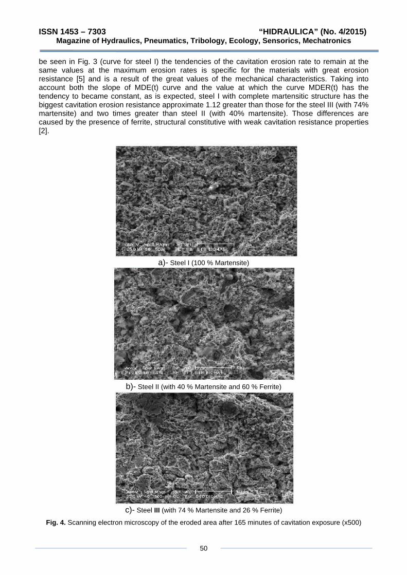
ISSN 1453 – 7303 “HIDRAULICA” (No. 4/2015) Magazine of Hydraulics, Pneumatics, Tribology, Ecology, Sensorics, Mechatronics
50
be seen in Fig. 3 (curve for steel I) the tendencies of the cavitation erosion rate to remain at the same values at the maximum erosion rates is specific for the materials with great erosion resistance [5] and is a result of the great values of the mechanical characteristics. Taking into account both the slope of MDE(t) curve and the value at which the curve MDER(t) has the tendency to became constant, as is expected, steel I with complete martensitic structure has the biggest cavitation erosion resistance approximate 1.12 greater than those for the steel III (with 74% martensite) and two times greater than steel II (with 40% martensite). Those differences are caused by the presence of ferrite, structural constitutive with weak cavitation resistance properties [2].
a)- Steel I (100 % Martensite)
b)- Steel II (with 40 % Martensite and 60 % Ferrite)
c)- Steel III (with 74 % Martensite and 26 % Ferrite)
Fig. 4. Scanning electron microscopy of the eroded area after 165 minutes of cavitation exposure (x500)

ISSN 1453 – 7303 “HIDRAULICA” (No. 4/2015) Magazine of Hydraulics, Pneumatics, Tribology, Ecology, Sensorics, Mechatronics
51
In Fig. 4 are presented pictures of the eroded area taken with scanning electron microscopy. Figs. 5 - 7 are images of the surface degradation of the samples, after 165 minutes of cavitation exposure, registered with a high definition camera (zoomed in 8 times). There are also presented the lines used for roughness measurements. The roughness parameters Ra, Rz and Rt, presented in these pictures have been registered with a MITUTOYO apparatus at the Timisoara National Institute for Research and Development for Welding and Material Testing [9], which has allowed the cartography of the measurement zones (see Fig. 8).
Fig. 5. Roughness for Steel I (100 % Martensite) before and after cavitation exposure
Fig. 6. Roughness for Steel II (with 40 % Martensite and 60 % Ferrite)

ISSN 1453 – 7303 “HIDRAULICA” (No. 4/2015) Magazine of Hydraulics, Pneumatics, Tribology, Ecology, Sensorics, Mechatronics
52
Fig. 7. Roughness for Steel III (with 74 % Martensite and 26 % Ferrite)
Fig. 8. Roughness before cavitation exposure

ISSN 1453 – 7303 “HIDRAULICA” (No. 4/2015) Magazine of Hydraulics, Pneumatics, Tribology, Ecology, Sensorics, Mechatronics
53
The values of the parameters Ra, Rz, Rt from fig. 5-8, reconfirm the increased resistance conferred by the structure with great content of martensite, respectively the progressive decrease of resistance depending on the increase quantity of ferrite. Figure 9 presents sections with an axial plan (perpendicular on the surface attacked by the cavitation) and the erosion maximum depth value Hmax which appear in this section. In comparison with the mean depth erosion (MDE) used in Fig. 1, the value Hmax have differences, especially for steel II (with 60% ferrite). The explanation is given by the small cavitation erosion resistance of the structural component ferrite which gives deep erosions in some particular area and so the value Hmax differ substantially from the mean depth and is closer to the roughness values measured with the Mitutoyo apparatus. On the contrary, for the steel I, with a structure formed exclusively of martensite, the difference between the MDE (at 165 minutes), Hmax and Rt is very reduced, as a consequence of increased cavitation resistance on this component.
Fig. 9. Aspects of the sectioned specimens: a) the manner in which the specimens were sectioned;
b) maximum depth erosion Hmax after 165 minutes of cavitation exposure in this section 5. Conclusions
The research presented in this paper shows that for the pieces having a constant and heavy exposure to cavitation erosion (such as hydraulic machinery runner or blades) it is preferable to use stainless steels with a great content of martensite in the structural constitution. In the case of duplex steels, with structures formed from martensite and ferrite, the ones with a smaller quantity of ferrite have the best behavior. The evaluation of the resistance to cavitation can be also done by measuring the roughness, especially the value Rt, which is enough close to Hmax (the maximum depth generated by cavitation). Even if the roughness measurements are easier to be done, we do not recommend modifying the prescription of the ASTM 32-2010 Standard which is more reliable.
Acknowledgement
The work is funded by the internal competition of research projects USAMVBT 2015.

ISSN 1453 – 7303 “HIDRAULICA” (No. 4/2015) Magazine of Hydraulics, Pneumatics, Tribology, Ecology, Sensorics, Mechatronics
54
References
[1] I. Anton, ”Cavitation”, Tom II, Romanian Academy Publishing House, Bucharest, 1985 (in Romanian); [2] I. Bordeaşu, “Cavitation Erosion of Materials”, Timisoara Polytechnic Publishing House, 2006, (in
Romanian); [3] I. Bordeaşu, I. Mitelea, “Cavitation Erosion Behavior for some Stainless Steels with Constant Nickel and
variable Chromium Content”, MP Materiall Testing, Issue 01, ISSN: 0025-530, pp. 53-58, 2012; [4] I. Bordeaşu, M.O. Popoviciu, “Cavitation Erosion Resistance for a Set of Stainless Steels Having 10 %
Nickel and Variable Chromium Concentrations”, “Hidraulica” (No. 1/2013), Magazine of Hydraulics, Pneumatics, Tribology, Ecology, Sensorics, Mechatronics, ISSN 1453 – 7303, pp.79-85;
[5] I. Bordeasu , M.O. Popoviciu, I. Mitelea I., LM. Micu, OV. Oanca, C. Bordeasu, L. Salcianu, C. Ghera, “Cavitation Erosion Resistance of Ampco 45 Bronze with Heat Treatments”, “Hidraulica” (No. 2/2014), Magazine of Hydraulics, Pneumatics, Tribology, Ecology, Sensorics, Mechatronics, ISSN 1453 – 7303, pp.53-61;
[6] M. Popoviciu, AF.Kuzman, “Contributions to the study of cavitation erosion on Kaplan turbine runners”, Conference “Hydroforum “, Gdansk, 1985;
[7] N. I. Palaev, Iu. U.Edel, -“Kavitatia v ghidroturbinah”, Masinostroenie, Leningrad, 1974; [8] A.D. Perenik , “Problema kavitatii”, Sudpromghiz, 1963; [9] O.V. Oanca, “Tehnici de optimizare a rezistenţei la eroziunea prin cavitaţie a unor aliaje CuAlNiFeMn
destinate execuţiei elicelor navale” Teza de doctorat, Timișoara, 2014; [10] M.M.Orakelasvili,„Iznosostoikost reaklivnih ghidroturbin”, Gosenergoizdat, 1960; [11] *** “Standard method of vibratory cavitation erosion test”, ASTM, Standard G32-10, 2010.

ISSN 1453 – 7303 “HIDRAULICA” (No. 4/2015) Magazine of Hydraulics, Pneumatics, Tribology, Ecology, Sensorics, Mechatronics
55
Multiplexed Delay Compensation and Circular Buffer Method for moving Average Filtering of Signal Acquired from Tactile Sensors in a
Mechatronics System for Walking Analysis
PhDc. Eng. Anghel CONSTANTIN1, Prof. Dr. Ing. Constantine DAVID2
1 Doctoral School of Valahia University Targoviste, 130105, Romania, e-mail: [email protected] 2Technological Education Institute of Central Macedonia -Serres, Greece, e-mail: [email protected]
Abstract: Traditional filtering performs very well when the frequency content of signal and noise do not overlap. When the noise bandwidth is completely separated from the signal bandwidth, the noise can be decreased easily by means of a linear filter. On the other hand, when the signal and noise bandwidth overlap and the noise amplitude is enough to seriously corrupt the signal, a traditional filter, designed to cancel the noise, besides might introduce signal cancellation or, at least, would result in signal distortion. The paper presents a multiplexed delay compensation and circular buffer method for moving average filtering of signals. The application refers to the measurement of the ground reaction force during walking using 20 tactile-sensors in order to calculate the caloric energy consumption of the human body. The proposed method is an improved version of a previous one, where a low-speed microprocessor was used and there was not enough time to complete the required calculations and corrections. The current results are very promising, as the error correction due to delay of the samples between sensors by applying the moving average filtering method and using as well circular buffer is minimized.
Keywords: DSP, ring buffer, circular buffer, tactile sensors
1. Introduction
Advanced technology and new generation industrial applications, both matured and under development, contribute substantially to the design, development, validation and integration of Intelligent Mechatronics Systems [1]. However in many mechatronics applications there is a major problem how to prepare and process sufficiently the signals acquired from the sensors. This research work aims at the calculation of the caloric energy that is consumed by a human body during walking. To achieve that the ground reaction forces (GRF) acting on the foot sole at walking are experimentally assessed. The signals we are looking for are acquired from appropriate touch sensors applied on the sole. The force data are used for further analysis, whereby interesting technical aspects and restrictions have to be considered as following:
The large number of sensors (10 on each foot) demands sampling and multiplexing digital analog conversion.
The high impedance sensors cause noise and there is need to signal filtering, etc.
Figure 1 illustrates graphically the signal acquisition set-up. The signals recorded from the sensors after proper conditioning are acquired by a microcontroller supported device. The analog multiplexer allows the use of a single analog digital converter with a 10 bits resolution, which is included in the microcontroller, for the 20 analog input channels. The closing and opening command for the analog switchers is performed by the means of 5 selection inputs commanded by the microcontroller. This sampling process within the time domain creates a delay of the observation moments for each channel, which is proportional to the number of that channel multiplied by the time needed for the conversion of each channel. This phenomenon introduces errors within the calculation needed by the processing in order to find out the powers developed by different compounds of the reaction force and the total caloric energy which is consumed. The maximum error shows up at the maximum frequency and at the sensor No. 20 as shown hereinafter.
(1)
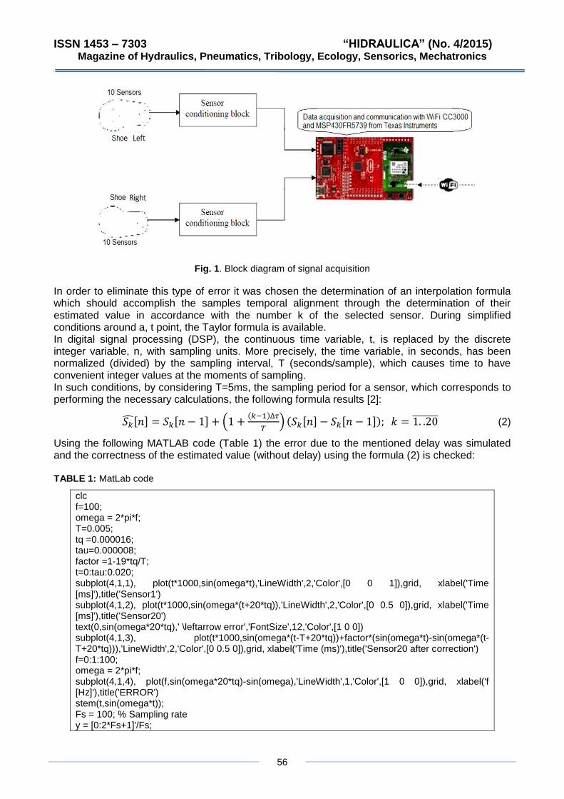
ISSN 1453 – 7303 “HIDRAULICA” (No. 4/2015) Magazine of Hydraulics, Pneumatics, Tribology, Ecology, Sensorics, Mechatronics
56
Fig. 1. Block diagram of signal acquisition
In order to eliminate this type of error it was chosen the determination of an interpolation formula which should accomplish the samples temporal alignment through the determination of their estimated value in accordance with the number k of the selected sensor. During simplified conditions around a, t point, the Taylor formula is available. In digital signal processing (DSP), the continuous time variable, t, is replaced by the discrete integer variable, n, with sampling units. More precisely, the time variable, in seconds, has been normalized (divided) by the sampling interval, T (seconds/sample), which causes time to have convenient integer values at the moments of sampling. In such conditions, by considering T=5ms, the sampling period for a sensor, which corresponds to performing the necessary calculations, the following formula results [2]:
(2)
Using the following MATLAB code (Table 1) the error due to the mentioned delay was simulated and the correctness of the estimated value (without delay) using the formula (2) is checked: TABLE 1: MatLab code
clc f=100; omega = 2*pi*f; T=0.005; tq =0.000016; tau=0.000008; factor =1-19*tq/T; t=0:tau:0.020; subplot(4,1,1), plot(t*1000,sin(omega*t),'LineWidth',2,'Color',[0 0 1]),grid, xlabel('Time [ms]'),title('Sensor1') subplot(4,1,2), plot(t*1000,sin(omega*(t+20*tq)),'LineWidth',2,'Color',[0 0.5 0]),grid, xlabel('Time [ms]'),title('Sensor20') text(0,sin(omega*20*tq),' \leftarrow error','FontSize',12,'Color',[1 0 0]) subplot(4,1,3), plot(t*1000,sin(omega*(t-T+20*tq))+factor*(sin(omega*t)-sin(omega*(t-T+20*tq))),'LineWidth',2,'Color',[0 0.5 0]),grid, xlabel('Time (ms)'),title('Sensor20 after correction') f=0:1:100; omega = 2*pi*f; subplot(4,1,4), plot(f,sin(omega*20*tq)-sin(omega),'LineWidth',1,'Color',[1 0 0]),grid, xlabel('f [Hz]'),title('ERROR') stem(t,sin(omega*t)); Fs = 100; % Sampling rate y = [0:2*Fs+1]'/Fs;

ISSN 1453 – 7303 “HIDRAULICA” (No. 4/2015) Magazine of Hydraulics, Pneumatics, Tribology, Ecology, Sensorics, Mechatronics
57
In Figure 2 the ground reaction force measurement from the sensor No1 and sensor No20 is shown, as well as the dependency of the frequency error.
Fig. 2. Signal from two sensors and the resulted frequency error
2. Filter implementation and methods
In practice the difference between simulation and real signal to be processed is the action of noise. Because the input amplifier of a signal conditioning system has high impedance the main component of the noise has 50Hz frequency due to the power line capacitive common mode coupled with other power lines belong to the environment. In order to minimize this influence a conditioning amplifier was designed in differential topology with antialiasing filter and a moving average digital filter using a circular buffer on the basis of a signal processing software was developed. Signal averaging is a signal processing technique applied in the time domain, intends to increase the strength of a signal relative to noise [3]. By averaging a set of replicate measurements, the signal-to-noise ratio, S/N, will be increased, ideally in proportion to the square root of the number of measurements [4]. If, x[n] is the input signal, y[n] is the output samples of the signal, M is the number of points used in the moving average window then the equation using only points on one side of the output sample is calculated as following:
(3)
For example, in an eight points moving average filter, ten points in the output signal is given by:
(4)
2.1 Recursive implementation
Based on equation (3) two adjacent output points [n] and y[n+1], can be calculated using the recursive fast calculus. After the first point is calculated in y[1], all other points can be found with only a single addition and subtraction per point. This can be expressed as the equation (5) declares:
(5)

ISSN 1453 – 7303 “HIDRAULICA” (No. 4/2015) Magazine of Hydraulics, Pneumatics, Tribology, Ecology, Sensorics, Mechatronics
58
Where:
and (6)
Before using the equation (3), the first point in the signal must be calculated using a standard summation.
Fig. 3. Standard summation scheme of the signal
In Figure 3, the average within a sampling region [4] is illustrated, rather than just being equal to the signal value at the sampling instant. A coherent averaging procedure can be perceived as a digital filtering process, and the frequency characteristics can be also investigated. In expression (7) through the z- transform, the transfer function of the filtering operation results in:
(7)
Where N is the number of elements in the average, and n is the number of samples in each response. This is a moving average low-pass filter as discussed earlier, where the output is a function of the preceding value with N samples. In practice, the filter does not operate on the time sequence but in the sweep sequence on corresponding samples. Basically the moving average filter is a convolution of the input signal with a rectangular pulse having an area of one. By the aid of a MatLab application the frequency response of the filter as shown in Fig. 4 can be calculated.

ISSN 1453 – 7303 “HIDRAULICA” (No. 4/2015) Magazine of Hydraulics, Pneumatics, Tribology, Ecology, Sensorics, Mechatronics
59
Fig. 4. Frequency response of the filter
The moving average filtering method proved to be a very good solution for many applications, it is optimal for reducing the noise while keeping the sharpest step response. The roll-off is very slow and the stop band attenuation is very bluff but the moving average filtering cannot separate one band of frequencies from another band [5]. In conclusion the moving average filtering has good performance in the time domain and poor performance in the frequency domain, and vice versa. In other words the moving average is an exceptionally good smoothing filter (the action in the time domain), but a bad low-pass filter (the action in the frequency domain).
2.2 Circular buffer implementation
In off-line processing, the entire input signal resides in the memory at the same time. This means for example, a doctor has the possibility to record the ground reaction force during human walking and analyze that afterward. Another example of off-line processing is medical imaging, such as computed tomography and MRI. This method supposes the existence of huge data recording and big memory support. In real-time processing, the result of output signal is produced at the same time that the input signal is being acquired. For example, this is needed in voice communication, radar or other applications where there is an indispensable demand to have the information immediately available, although it can be delayed by a short amount. For instance, a 10 millisecond delay in a telephone call cannot be detected by the speaker or listener. Real-time applications input a sample, perform the algorithm of calculus, and output a sample, over-and-over [5]. To calculate the output sample, we must have access to a certain number of the most recent samples from the input. For example, we suppose eight coefficients in this filter. This means, it is required to know the value a1,..,a7 of the eight most recent samples from the input signal, x[n], x[n+1],…,x[n+7]. These eight samples must be stored in memory and continually updated as new samples are acquired. The most satisfactory solution for memory managing is to use a circular buffering presented as principle in the Figure 5.

ISSN 1453 – 7303 “HIDRAULICA” (No. 4/2015) Magazine of Hydraulics, Pneumatics, Tribology, Ecology, Sensorics, Mechatronics
60
Fig. 5. Circular buffering principle scheme In table 2 below a short listing of the C code used in the application is demonstrated. The code aims at the real-time filtering of the digital data acquired from the ground reaction force, which is recorded by means of 20 tactile sensors during walking. TABLE 2: C code listing
#define BUFFER_SIZE 16 typedefstructcircular_buffer { int buffer[BUFFER_SIZE]; volatileunsignedint head; volatileunsignedintrear; }ring_buffer; ring_buffermy_buf = { {0}, 0, 0 }; /*******************************************************************************/ voidstore_in_buffer(int data) { unsignedint next = (unsignedint)(my_buf.head + 1) % BUFFER_SIZE; if (next != my_buf.rear) { my_buf.buffer[my_buf.head] = data; my_buf.head = next; } /*******************************************************************************/
for (index_filtru=0;index_filtru<BUFFER_SIZE;index_filtru++) { if (my_buf.head == my_buf.rear) { } else { data = my_buf.buffer[my_buf.rear]; my_buf.tail = (unsignedint)(my_buf.rear + 1) % BUFFER_SIZE; } dADC1 =(double)data, dSum=dSum+dADC1; }

ISSN 1453 – 7303 “HIDRAULICA” (No. 4/2015) Magazine of Hydraulics, Pneumatics, Tribology, Ecology, Sensorics, Mechatronics
61
4. Conclusions
The moving average method is the most common filtering technique in DSP, mainly because it is the simplest digital filter to understand and to use and it is optimum for a common task because of reducing random noise, while at the same time retaining a sharp step response [6]. This makes it the premier filter for time domain encoded signals. However, the moving average is the worst filter for frequency domain encoded signals because it does not have the ability to separate one band of frequencies from another. Simultaneous Sampling eliminates time skew between channels, simplifies however both time and frequency based analysis techniques. Multiplexed Sampling channels are sampled sequentially requiring also software correction for detecting certain patterns.
Acknowledgements
This paper has been prepared with the financial support of the project “Quality European Doctorate - EURODOC”, Contract no. POSDRU/187/1.5/S/155450, project co-financed by the European Social Fund through the Sectoral Operational Programme “Human Resources Development” 2007-2013.
References
[1] Gh. I. Gheorghe, “Adaptronica Sistemelor Inteligente”, AGIR Publishing House, Bucharest, Romania, 2014, ISBN: 978-973-720-509-4, p.15, 2014;
[2] S. Pasca, R. Strungaru, A. Constantin, G. Capris, “New Data Acquisition and Processing Methods for Resistive Sensors in Pedometric Measurement Systems”, Nonlinear Optics, Quantum Optics: Concepts in Modern Optics; 2009, NLOQO 39.2-3, pp. 117-136;
[3] Ed. Joseph D. Bronzino, “The Biomedical Engineering Handbook, Second Edition”, CRC Press LLC, ISBN 0-8493-0461-X, pp.238, 988 2000;
[4] S. D. Stearns and D. R. Hush, “Digital Signal Analysis”, 2nd Ed., Englewood Cliffs, NJ: Prentice Hall, 1990;
[5] Texas Instruments, Inc., TMS320C55x Chip Support Library API Reference Guide, Literature no. SPRU433J, Sep. 2004;
[6] R. Rădoi, I. Duțu, “Virtual instrument for plotting servo-valves characteristics after significant maintenance operations”, In: Hidraulica no. 1/ 2013, pp. 86-89.

ISSN 1453 – 7303 “HIDRAULICA” (No. 4/2015) Magazine of Hydraulics, Pneumatics, Tribology, Ecology, Sensorics, Mechatronics
62
Effects of Turbo Charging of Spark Ignition Engines
Aman GUPTA1, Sunny NARAYAN2
1 Indus University, India, [email protected] 2 Indus University, India, [email protected]
Abstract: Turbocharging is an important method that is aimed at achieving maximum mechanical efficiency & fuel-economy, both simultaneously in automobiles. The principle objective of turbo charging is to increase the power output per volume and cost of engine. A fact that a turbocharger increases the mass of air in the cylinder and consequently allows more fuels to be burnt, improves the volumetric efficiency of the engine and simultaneously improves engine efficiency by a small but worthwhile amount. Turbochargers are commonly being used on diesel engines for many years. In contrast only a few petrol engines have been turbocharged until recently and it is unlikely that a large fraction of the world petrol engine will be so equipped. There would be a tremendous growth in demand of Gasoline downsizing, in next few years. The present work aims at analyzing the various benefits associated with Turbo charging in SI engines and designing it for future automotive engines. Design calculations were performed to compare improvements in performance of engine with and without turbocharging which highlight the advantages of turbocharging process.
Keywords: S.I. Engines, Turbo charging
1. Introduction
A turbocharger basically consists of a compressor and a turbine coupled on a common shaft [1].The exhaust gases from the engine are directed by the turbine inlet casing on to the blades of the turbine and subsequently discharged to atmosphere through a turbine outlet casing [2].The exhaust gases are utilized in the turbine to drive the compressor, which compresses the air and directs it to the engine induction manifold, to supply the engine cylinders with air of higher density than is available to a naturally aspirated engine [3]. The higher value of air-pressure achieved using a turbo-unit is called Boost-pressure [4].There exist a number of different types of compressors and turbines, but few of these are ideally suitable to form the basis of an exhaust gas driven supercharging system. The combination of a single stage centrifugal compressor and a single stage axial flow or radial flow turbine is almost universally used in turbochargers [5].The former type is used for medium and large size engines, while the latter type is used for small engines of automotive type. Some merits of this technology include: 1. Increase the fuel volumetric efficiency by about 30% to 40%. 2. Increase the number of power stroke i.e. increase the final output. Some demerits include: 1. A disadvantage of turbo charger is its resistance to high temperature at high load, which imposes to increase equivalent ratio (enrichment). 2. The main disadvantage in the turbine inertia and the corresponding long response time needed to obtain the supercharging pressure.
2. Turbocharging in S.I. engines
In SI engines, fuel and air are pre-mixed before the air enters the cylinder of petrol engine. Whether a carburetor or manifold petrol injection system is used, cylinder comprises of homogeneous air and fuel mixture, the proportion of fuel being carefully controlled [6].The homogeneous mixture is ignited by the spark plug. Unlike diesel engine the rate at which combustion proceeds is governed by heat and mass transfer from an area that is burning to an area that is not, and temperature increase due to continued compression thus flame advances across the combustion chamber, from the spark plug until all the fuel is burned [7].

ISSN 1453 – 7303 “HIDRAULICA” (No. 4/2015) Magazine nics
63
of Hydraulics, Pneumatics, Tribology, Ecology, Sensorics, Mechatro
Fig. 1. Sketch of a turbocharged SI-engine
Self ignition is avoided by low compression ratios, enough to hold the temperature of mixture below the self ignition point of the fuel, and by self ignition temperature [8]. The rate at which the flame progresses is governed by local turbulence, heat transfer between burning and unburned region, compression heating of the unburned gas due to piston motion and expansion of burning mixture, air/fuel ratio and heat transfer to the surrounding walls [9]. Since the unburnt gas that is removed from the advancing flame front is heated by compression and to some extent by radiation etc. [10].This gas can reach its self ignition temperature before the flame front arrives, thus increasing the chances of knocking in the end gas region 11].This extremely rapid combustion generates a high rate of pressure rise in the cylinder, the impulse of force causing the bearing to knock, generally referred to as detonation [12].
3. Parts of Turbocharger
3.1 Turbine [13]
The turbine wheel is made from a high nickel super-alloy investment casting. This method produces accurate turbine blade sections and forms. Larger units are cast individually. For smaller sizes the foundry will cast multiple wheels using a tree configuration.
Fig. 2. Sketch of a turbine wheel

ISSN 1453 – 7303 “HIDRAULICA” (No. 4/2015) Magazine of Hydraulics, Pneumatics, Tribology, Ecology, Sensorics, Mechatronics
64
3.2 Compressor [14]
Compressor impellers are produced using a variant of the aluminum investment casting process. A rubber former is made to replicate the impeller around which a casting mould is created. The rubber former can then be extracted from the mould into which the metal is poured. Accurate blade sections and profiles are important in achieving compressor performance. Back face profile machining optimizes impeller stress conditions. Boring to tight tolerance and burnishing assist balancing and fatigue resistance. The impeller is located on the shaft assembly using a threaded nut. Compressor housings are also made in cast aluminum (cast iron for high-pressure applications). Various grades are used to suit the application. Both gravity die and sand casting techniques are used. Profile machining to match the developed compressor blade shape is important to achieve performance consistency.
Fig. 3. Sketch of a compressor wheel
Fig. 4. Sketch of a P-V curve turbocharged SI-engine

ISSN 1453 – 7303 “HIDRAULICA” (No. 4/2015) Magazine of Hydraulics, Pneumatics, Tribology, Ecology, Sensorics, Mechatronics
65
4. Conclusion
This work compares the engine performance of a spark ignition engine with and without use of turbocharging system. A decrease in specific fuel consumption is observed with increased torque output and thermal efficiency. In the 1980s, turbocharged cars were difficult to handle. The tuned engines fitted to the cars, and the often primitive turbocharger technology meant that power delivery was unpredictable and the engine often suddenly delivered a huge boost in power at certain speeds.. As turbocharger technology improved, it became possible to produce turbocharged engines with a smoother, more predictable but just as effective power delivery. Today, turbo charging is most commonly used on two types of engines: Gasoline engines in high-performance automobiles and diesel engines in transportation and other industrial equipment. Small cars in particular benefit from this technology, as there is often little room to fit a larger-output (and physically larger) engine. In future, to meet U.S. emission regulations, injector systems will have to be optimized with increased functionalities, multiple injection strategies and increase pressures (up to 2000 bars or more). However improved combustion systems will have to be supplemented with after - treatment techniques like selective catalytic reduction (SCR) for NOx reduction and state of art particulate filters. Turbo charging would be adopted much faster in downsized engines for entry level vehicles, on account of their low costs.
References
[1] Payri F, Serrano JR, Piqueras P, García-Afonso O. ,''Performance analysis of a turbocharged heavy duty diesel engine with a pre-turbo diesel particulate filter configuration'', SAE Int J Engines 2011;4(2):2559-72;
[2] Bermúdez V, Luj_an JM, Piqueras P, Campos D., ''Pollutants emission and particle behavior in a pre-turbo aftertreatment light-duty diesel engine'', Energy, 2014;66:509-22;
[3] Bermúdez V, Serrano JR, Piqueras P, García-Afonso O. ,''Assessment by means of gas dynamic modelling of a pre-turbo diesel particulate filter configuration in a turbocharged HSDI diesel engine under full-load transient operation'', P I Mech Eng D-J Aut 2011;225(9):1134-55;
[4] Serrano JR, Arnau FJ, Dolz V, Piqueras P.,'' Methodology for characterization and simulation of turbocharged diesel engines combustion during transient operation. Part 1: data acquisition and post-processing'', Appl Therm Eng 2009;29(1):142e9;
[5] Payri F, Benajes J, Galindo J, Serrano JR.,'' Modelling of turbocharged diesel engines in transient operation. Part 2: wave action models for calculating the operation in a high speed direct injection engine'', P I Mech Eng D-J Aut 2002; 216:479-93;
[6] Serrano JR, Climent H, Piqueras P, Angiolini E.,'' Analysis of fluid-dynamic guidelines in diesel particulate filter sizing for fuel consumption reduction in post-turbo and pre-turbo placement'', Appl. Energ. 2014;132:507-23;
[7] Jenny E, Hansel J, Mayer A.,'' The transient behavior of supercharged passenger car diesel engines fitted with particulate traps'', In: SAE Technical Paper890171; 1989;
[8] www.openwam.org; [9] Serrano JR, Arnau FJ, Dolz V, Tiseira A, Lejeune M, Auffret N.,'' Analysis of the capabilities of a two-
stage turbocharging system to fulfill the US2007 antipollution directive for heavy duty diesel engines'', Int J Automot Techn 2008;9(3):277-88;
[10] Hiereth H.,''Car tests with a free-running pressure-wave charger -A study for an advanced supercharging system'', In: SAE Technical Paper 890453; 1989;
[11] Tourlonias P, Koltsakis GC. ,''Model-based comparative study of Euro 6 diesel after treatment concepts, focusing on fuel consumption'', Int J Engine Res, 2011;12:238-51;
[12] Serrano JR, Guardiola C, Piqueras P, Angiolini E. ,''Analysis of the after treatment sizing for pre-turbo DPF and DOC exhaust line configuration'', SAE Tech Pap 2014-01-149;
[13] Dragomirescu A., ''Configurations of flow induced by a fan impeller without impeller casing'', Hiraulica no 3, 2015;
[14] Budea S., Simionescu S., ''Numerical simulation of viscous fluid flow by sealing labyrinth'', Hiraulica no 1, 2014.

ISSN 1453 – 7303 “HIDRAULICA” (No. 4/2015) Magazine of Hydraulics, Pneumatics, Tribology, Ecology, Sensorics, Mechatronics
66
Validation of a Multiple Linear Regression Model
Marin RUSĂNESCU1, Anca Alexandra PURCĂREA2
1 Valplast Industry Bucharest, [email protected] 2 Politehnica University of Bucharest, Faculty of Entrepreneurship, Business Engineering and Management,
Romania
Abstract: In this paper, we present a model of multiple linear regressions for the margin trade.
Keywords: inventory, performance of organization, margin trade, multiple linear regression model
1. Introduction
In the current economy, it has become imperative to have a professional management of the firms. The relationship between inventory management and organizational performance is fairly debated. Overall it is accepted that good management of inventories influences the performance of the organization. However, all stocks were not analyzed in detail. It is proposed to establish a framework for analyzing the influence of the inventories on the performance of organization. Beside the method MRP, that is another method to control the inventory [1] and the method ABC, that is a method of control for inventories [2], we can control inventories even at a summary level using a model of relation between a dependent variable and others dependent variables, a model that we will propose below.
2. The proposal of a multiple linear regression model
It is known that the performance of the organization is primarily measured in financial terms. For example, the index Gartner, according to [3], has about 10 years old when calculating and aims to make a ranking of the top 25 supply chain companies, ranking focuses on idea-driven application, has two main components, namely 50% based on the opinion of two panels of voters and 50% on financial metrics such as: ROA (return on assets), inventory turnover and income growth. We analyze the impact of inventories on the performance of the organization financially. Inventory turnover defined, shows how well managed stocks are, where big is said to be good. But this opinion should be relaxed because of the possibility to rotate inventories less so to have a lower value of this indicator and simultaneously to have a gross margin greater unlike the version in which you have an inventory turnover greater and gross margin small. The inventory turnover is different on sectors, industries, within the branches, may be different from companies operating in the field. In order to obtain a regression function, seek to highlight the inventory turnover in conjunction with inventory growth rate, rate margin / cost of goods sold and commercial margin was calculated. It is tried to show that the commercial margin is a function of inventory turnover, inventory growth rate, rate margin / cost of goods sold, based on data analyzed company operating in industrial processing branch. Commercial margin is the rate of financial performance and inventories turnover is a metric important to inventory, supply activity; it can be global or types of stocks; rate margin / cost of goods sold is the ratio between margin and cost of goods sold, also an important metric of supply, the rate of growth inventory is relevant to the situation of inventory and succeed in modeling of commercial margin based on inventory turnover, rate margin / cost of goods sold and inventory growth rates demonstrate the influence of supply on performance. All three dependent variables make sense to influence the commercial margin. It is proposed as a model for determining the rate of commercial margin, a model where the dependent variable is the rate of commercial margin and as independent variables: inventory turnover, rate margin / cost of goods sold, inventory growth rate.

ISSN 1453 – 7303 “HIDRAULICA” (No. 4/2015) Magazine of Hydraulics, Pneumatics, Tribology, Ecology, Sensorics, Mechatronics
y=α0+α1X1+α2X2+α3X3+ε[4]
• y is the dependent variable (explained endogenous outcome) and the rate of commercial margin • x is the vector of independent variables (explanatory exogenous), the size 1×p, in this case X 1-inventory turnover, X2-rate margin/cost of goods sold X3- inventory growth rate, • α is the vector coefficients of size p × 1, the model parameters, • ε is a variable interpreted as an error.
3. Validation of the model
In this paper we try to analyze the influence of the inventories on the performance of the financial statements of the company. We chose to analyze the data of a company; for confidentiality reasons we noted the enterprise CA = analyzed. We chose its data from the 2009-2013 periods to extract conclusion in as well founded. To see the influence of inventories we show a table with primary data, Table 1.
TABLE 1: Primary data
Lei-absolute value 2009 2010 2011 2012 2013
Turnover 69,115,487 62,304,542 71,453,534 70,673,051 98,376,866
Cost of goods sold 50,459,012 49,149,779 57,989,330 56,272,156 76,688,403
Commercial margin 18,656,475 13,154,763 13,464,204 14,400,894 21,688,463
Inventory 5,801,992 8,900,550 10,759,210 11,433,702 11,159,340
Average of inventory 7,353,042 7,351,271 9,829,880 11,096,456 11,296,521
Inventory growth rate 0.65 1.53 1.21 1.06 0.98
Rata margin/cost of
goods sold 0.37 0.27 0.23 0.26 0.28
Rata of commercial
MARGIN 0.27 0.21 0.19 0.20 0.22
Inventory turnover 6.86 6.69 5.90 5.07 6.79
Inventories for year
2008=8904091
Company performance is the commercial margin rate calculated by the formula
Turnover
margin Commercialmargin commercial of Rate = (1),[5]
Commercial margin rate is also a dependent variable explained by some inventory rate:
year previousInventory
yearcurent Inventory sinventoriein increase Rate = (2),
sold goods ofCost
margin Commercialsold goods ofcost on margin Rate = (3),
67

ISSN 1453 – 7303 “HIDRAULICA” (No. 4/2015) Mechatronics
68
Magazine of Hydraulics, Pneumatics, Tribology, Ecology, Sensorics,
inventory of valueAverage
sold goods ofCost turnoverInventory = (4), [6]
In order to determine a linear regression model the commercial margin rate based on inventory turnover, rate margin / cost of goods sold, inventory growth rate, these data are presented in Table 2. TABLE 2: The rate of inventory turnover depending on commercial margin, rate margin / cost of goods sold and inventory growth rate in 2009-2013 for the company analyzed
Year Rate of commercial
margin Inventory turnover Rate margin/Cost of
goods sold Inventory growth rate
2009 0.27 6.86 0.37 0.65
2010 0.21 6.69 0.27 1.53
2011 0.19 5.90 0.23 1.21
2012 0.20 5.07 0.26 1.06
2013 0.22 6.79 0.28 0.98
After analyzing the data in Data Analysis, Analysis Tools, regression function following data were found, as shown in Table 3. TABLE 3: Regression model
SUMMARY OUTPUT
Regression Statistics
Multiple R 0.999621
R Square 0.999243 Adjusted R Square 0.996971 Standard Error 0.001702
Observations 5
ANOVA
Df SS MS F Significance
F
Regression 3 0.003821 0.001274 439.8718 0.035032
Residual 1 2.9E-06 2.9E-06
Total 4 0.003824
Coefficients Standard
Error t Stat P-value Lower 95% Upper 95%
Lower 95.0%
Upper 95.0%
Intercept 0.049989 0.010323 4.84257 0.129641 -0.08117 0.181152 -0.08117 0.181152
X Variable 1 0.000324 0.001631 0.198454 0.875281 -0.0204 0.021045 -0.0204 0.021045
X Variable 2 0.588665 0.034965 16.83584 0.037769 0.144392 1.032937 0.144392 1.032937
X Variable 3 0.000855 0.004631 0.184565 0.88381 -0.05799 0.059695 -0.05799 0.059695
RESIDUAL OUTPUT PROBABILITY OUTPUT
Observation Predicted Y Residuals Standard Residuals Percentile Y
1 0.270417 -0.00048 -0.56971 10 0.188433
2 0.211018 0.000119 0.139677 30 0.203768
3 0.18961 -0.00118 -1.38302 50 0.211137
4 0.203186 0.000581 0.68339 70 0.220463
5 0.219502 0.000961 1.129666 90 0.269932

ISSN 1453 – 7303 “HIDRAULICA” (No. 4/2015) Magazine of Hydraulics, Pneumatics, Tribology, Ecology, Sensorics, Mechatronics
69
Analyzing the data shows that there is a strong link between variables, pointer Multiple R = 0.999621, it is close to the maximum possible one, and according R Square = 0.999243 variance variable rate commercial margin is explained by the three independent variables- inventory turnover, rate margin / cost of goods sold and inventory growth rate in the proportion of 99.9243%, which translates into the fact that the three independent variables strongly influence trading margin rate. Interpretation of the F is required to validate the regression model, [4]; there are 2 assumptions: H0: α1 = α2 = α3 = 0 H1: there is at least one nonzero coefficient αi. This test refers to all independent variables (H0 does not refer to the term free), considering that the whole significance of this test verifies regressions. Significance F - sided probability is critical and the resulting value is lower than the materiality threshold set, then the null hypothesis in favor of the alternative hypothesis; Statistics F test is obtained as a ratio of the average of squared deviations from the average of squared deviations from regression and residue, calculated with the appropriate degrees of freedom. If the test F has a high value and the value corresponding Significance F statistics is low (less than 0.05), the independent variables explain the variation in the dependent variable and vice versa. In this case the value of F is 439.8718 (is large), and the Significance F is 0.035032, is less than 0.05 materiality. It follows that the null hypothesis in favor of the alternative hypothesis H1, the model is valid. The values of these coefficients are: α0 = 0.049989 (free term) α1 = 0.000324 α2 = 0.588665 α3 = 0.00085 It follows that the dependent variable variation of the three independent variables takes the form of multiple linear regression equations of the form y=0.049989 + 0.000324x1 + 0.588665x2 + 0.000855x3 In terms of the regression equation graphically expressed in Figure 1 it is of the following form:
Fig. 1. The graphical representation of the equation, normal probability
This means that the group has a normal probability. We have the possibility that the data available in the future to make a forecast for values of commercial margin rate, thanks to the regression function above. This verifies the multiple linear regression model of the form y = α0+α1x1+α2x2+α3x3+ε

ISSN 1453 – 7303 “HIDRAULICA” (No. 4/2015) Magazine of Hydraulics, Pneumatics, Tribology, Ecology, Sensorics, Mechatronics
70
Conclusions
In this paper we have established a strong link between the rate of performance, margin rate commercial and three dependent variables - inventory turnover, rate margin / cost of goods sold, inventory growth rate - setting a model for the future of the dependent variable according to three independent variables. We can observe that this model can be performed by the supply system, as a part of the enterprise, that it is a rational system, that it has a goal to obtain profit, [7].
References
[1] Rusănescu, M., (2014a), "Material requirements planning, inventory control system in industry." Network impact (2014): p. 21. ISSN 1453 – 7303 “Hidraulica” (No. 1/2014) Magazine of Hydraulics, Pneumatics, Tribology, Ecology, Sensorics, Mechatronics;
[2] Rusănescu, M. (2014b), “ABC analysis, model for classifying inventory”. Loads an automated system using vacuum technology, p. 17. ISSN 1453 – 7303 “Hidraulica” (No. 2/2014) Magazine of Hydraulics, Pneumatics, Tribology, Ecology, Sensorics, Mechatronics;
[3] http://www.gartner.com/imagesrv/summits/docs/na/supply-chain/Gartner-2013-SupplyChainTop25.pdf; [4] http://thor.info.uaic.ro/~val/statistica/StatWork_8.pdf; [5] Brezeanu, P., Boştinaru, A., Prăjişteanu, B., (2003) Diagnostic financiar Instrumente de analiză
financiară, Bucharest, Economic Publishing House; [6] Jacobs, F.R., Chase, R.B., (2013), Operations and Supply Chain Management: The Core McGraw-Hill
Third Edition; [7] Rusanescu, M., Purcarea, A. A., & Rusanescu, C. O. (2013, November), “Comparative analysis of
different approaches to industrial organization as a system”. In International Conference on Management and Industrial Engineering (No. 6, p. 395), Niculescu Publishing House.

ISSN 1453 – 7303 “HIDRAULICA” (No. 4/2015) Magazine of Hydraulics, Pneumatics, Tribology, Ecology, Sensorics, Mechatronics
71
Using Load Sensing Control Systems to Increase Energy Efficiency of Hydrostatic Transmissions
PhD. Eng. Corneliu CRISTESCU1, Lecturer PhD. Eng. Lavinia Madalina MICU2, PhD. Eng. Catalin DUMITRESCU1, PhD. Student Eng. Petrica KREVEY1
1 Hydraulics and Pneumatics Research Institute INOE 2000-IHP, Bucharest, Romania, [email protected]
2 Banat`s University of Agricultural Sciences and Veterinary Medicine “King Michael I of Romania” in Timisoara (USAMVBT), [email protected]
Abstract: This paper makes a pleading reasoning the promotion of devices type "Load sensing" to control the flow and pressure in hydrostatic drive systems, in order to increase their energy efficiency. There are shown the operating principle, typical basic diagrams and some industrial applications. There is also shown a hydraulic diagram developed in INOE 2000-IHP, which is to be tested in the Laboratory of Hydraulics of the Institute.
Keywords: load sensing, hydrostatic transmissions, regulator, energy efficiency
1. Introduction
There are well known the great advantages of using hydrostatic transmissions, which in addition to high power density per kilogram of equipment, in combination with electronics provide a great flexibility and very broad possibilities for automation of drive processes. There are situations where electronics cannot be used to its full capabilities, especially in mobile equipment/ machinery which also have heavy-duty regimes, such as shovels etc. A most current issue is energy saving, especially saving of fossil fuels, which are on the verge of depletion globally. Therefore, increasing energy efficiency of devices, machinery and equipment, particularly the mobile ones, including the hydrostatic drive ones, is required acutely. The overwhelming majority of hydrostatic drives must provide variable speed at hydraulically driven working mechanisms and, consequently, variable flow at hydraulic motor of the driven mechanism, and also control of working pressures. The most efficient way in terms of energy for ensuring variable flow is for the pump supplying such flow to have adjustable / variable capacity / displacement. To this end, there have been developed a couple of devices for adjustment of capacity / displacement of positive displacement pumps and therefore adjustment of flow and pressure, but also power adjustment. There are a variety of regulators which, according to the way they reduce energy losses in the system, are classified into: pressure regulators and power regulators. Regulators are automatic devices for adjustment of displacement; during operation they do not require human operator intervention. They are mounted directly onto the pump or motor body, and adjustment of displacement is achieved under the effect of steering fluid pressure, fluid which can be collected from inside or outside the body [1]. Pressure regulators maintain a constant (or almost constant) pressure inside the circuit as long as the total flow rate demanded by consumers is lower than "breaking" flow rate. They are particularly useful when consumers of the system require variable flow rates. The existence of a pressure regulator causes the pump to provide a flow rate in line with requirements of the consumers in the system; it prevents the conversion into heat of certain part of the energy supplied by the pump as a result of excess fluid spilling toward the tank via system safety valve, as it happens in systems equipped with fixed displacement pump [2]. One particularly interesting version of pressure regulator is the one in which the regulators track actual variations in the load of working parts, that is they are regulators/compensators sensitive to

ISSN 1453 – 7303 “HIDRAULICA” (No. 4/2015) Magazine of Hydraulics, Pneumatics, Tribology, Ecology, Sensorics, Mechatronics
72
load variations, also known as devices / compensators type "Load sensing", which will be discussed below.
2. Operating principle of load sensing type devices
Load sensing type devices have emerged from the desire to improve the energy balance of hydrostatic drive systems. Equipping a variable capacity/displacement pump with such a device makes the flow and pressure along its discharge / working circuit be in line with requirements of the motor in the system; thus, there are always provided speed and torque, or force, needed at the output element of the motor. Many companies active in the field of fluid power have developed such devices, with very good practical outcomes [3], [4], [5]. Control based on load sensing is a type of control of a variable displacement pump used in hydraulic drive open circuits [6].
Basically, this controller is made up of the same components as a piloted pressure regulator. The difference is that in this case for the level of “pressure balance” there is made a comparison between the pressure
force Spx and the force developed by the
pressure Sp y , plus force of balance
adjustment spring, where S is surface of “pressure balance” spool valve. Pressure
yp must be collected as close to the motor
as possible; to this end, there can be used a circuit selector consisting of two one-way valves, Figure 1. Presence of the pressure
force Sp y in the equilibrium equation of
forces acting on the spool valve determines changes in control pressure, so that the latter could be permanently in line with the pressure required by the motor.
Fig. 1. Basic diagram with Load Sensing
This is the reason why these regulators have been named pressure regulators / compensators that track load variations. The adjustment spring (rather a spring for returning the spool valve to the neutral position) in the absence of pressures yp si xp is dimensioned such that pressure
difference yx ppp be enough for the balance spool valve to pass from neutral position (0) to
position (1): normal MPa. 2...1p When the main directional control valve in the system (the directional control valve serving the motor, in this case a 4-port and 3-position directional control valve) is in the neutral position (position 0) pilot pressure yp is zero. In order for the flow discharged by the pump to be null (in this
case the consumer does not require flow) it is necessary that cylinder rod be fully emerged; hence the balance spool valve must be maintained in position (1), and consequently ppr . As the value of p is very small, flow losses and friction moments are almost eliminated in their entirety, which reduces heat generation and power consumption even more.

ISSN 1453 – 7303 “HIDRAULICA” (No. 4/2015) Magazine of Hydraulics, Pneumatics, Tribology, Ecology, Sensorics, Mechatronics
73
When the main directional control valve executes one of the side positions (1) or (2), flow inside the circuit is adjusted using the throttle Dr; pressure loss on this equipment is:
,mrDr ppp (1)
where mp is pressure inside the motor active chamber. When writing the above relation load loss
in directional control valve was neglected. Since mrx ppp yp and , it follows that load loss in
throttle is p itself. It is known that the flow rate is calculated according to the following relation:
(2)
where: Q is flow rate in l/min, S is drain hole section in cm2, ρ is fluid density in kg/cm3, C is orifice flow coefficient (rank 0.72), and Δp is pressure difference at section holes, in bar. Since load loss in throttle p is very small, power loss imputable to the throttle is negligible and energy efficiency of the system is significantly improved. Moreover, this load loss remains constant even if the load of the motor in the system varies. The flow rate, respectively the speed at the working element is thus kept constant, regardless of load variation.
3. Basic diagrams and applications of load sensing devices
In scientific literature there are many examples of using control devices type load sensing, there being many companies that have created their own schematic diagrams and systems.
3.1. Hydraulic diagrams with Load sensing
Figure 2 presents a Load Sensing hydraulic control system, for linear motion (linear hydraulic motor), where both pressure and pump flow adapt to the conditions required by the consumer, based on pressure drop through proportional solenoids (1). In order to maintain the required pressure in the hydraulic cylinder (4), the variable displacement pump with Load Sensing type device (2) changes its geometric displacement volume, so that the flow of oil coming from the tank (3) to maintain constant pressure drop, that is constant speed at the cylinder rod, whatever the variation of resistant forces. Load Sensing helps to increase energy efficiency, because power losses are reduced [7].
Fig. 2. Linear motion control with Load Sensing device
Fig. 3. Rotary motion control with Load Sensing device

ISSN 1453 – 7303 “HIDRAULICA” (No. 4/2015) Magazine of Hydraulics, Pneumatics, Tribology, Ecology, Sensorics, Mechatronics
74
Figure 3 presents another Load Sensing hydraulic control system, for rotary motion (rotary hydraulic motor) of a hydraulically driven winch [8]. The Load sensing device detects variation in work load by measuring the pressure, and adjusts pump flow to the requirements of the installation, achieving thus optimization of hydraulic drive efficiency. The system compares the pressure P2, downstream of the throttle Sr, necessary to the hydraulic motor, with pump discharge pressure P1, and through this "pressure balance" it maintains constant pressure drop ΔP = P2 – P1, that is, according to the calculus relationship of flow shown above, maintains constant flow respectively working speed, regardless of the variation of work load. A Load Sensing control system belonging to MOOG is shown in Figures 4 and 5; on principle, it is a flow and pressure regulator / compensator. The system is based on a variable flow pump [3, 4], a variable throttle (hydraulic resistance) (1) and a pressure balance with a slide valve (7), comparing the pressures upstream and downstream of the throttle valve, the pressure drop being typically 10...12 bar, and according to some authors, up to no more than 20 bar. Figure 4 presents the pump equipped with Load Sensing type device, and Figure 5 shows the schematic diagram of the system [9].
Fig. 4. Pump with Load Sensing device
Fig. 5. Schematic diagram of Load Sensing pump
As one can seen in the diagram in Figure 4, the Load sensing device is simultaneously a flow and pressure regulator / compensator. Flow is adjusted by use of throttle 1, and pressure by use of valve 6. The function of pressure control is performed identically to the pressure regulators. Pump displacement is proportional to the throttle 1 opening. The pressure upstream of the throttle 1 is taken over and it acts on the lower area of the slide valve 7, and the one downstream - on the upper area. The pressure drop in the throttle 1 and the spring 8 together generate balance of the slide valve 7. Changing the throttle 1 setting entails change in the pressure difference between upstream and downstream of the throttle, putting the slide valve 7 out of balance, change in position of the piston 8, and hence in the pump capacity. Changing the pump capacity/displacement entails change in the pump flow, to the amount that produces the pressure drop preset by the throttle 1. Figure 6 presents a hydraulic diagram with Load Sensing type device designed in INOE 2000-IHP, which has been designed in order to control the speed of descent of the masses / weights, to a laboratory experimental model of a load lowering-lifting installation (crane). The experimental model has an actuation based on a fixed-displacement hydraulic rotary motor. The fixed-displacement pump, originally planned, is to be replaced with a variable-displacement pump, equipped with a Load Sensing type device [10]. Testing the below presented hydrostatic drive diagram in the Laboratory of General Hydraulics within INOE 2000-IHP will give the opportunity to improve it, if necessary, and in the end will lead to validation of the proposed solution, which has two ways to improve energy efficiency of hydrostatic drive systems: first- using Load Sensing type devices, and second- the concept of energy recovery.

ISSN 1453 – 7303 “HIDRAULICA” (No. 4/2015) Magazine of Hydraulics, Pneumatics, Tribology, Ecology, Sensorics, Mechatronics
75
Fig. 6. Hydraulic diagram with Load Sensing type device designed in INOE 2000-IHP
3.2. Industrial applications
Worldwide, there are a lot of industrial applications using Load sensing type devices/compensators. Thus, the company Bosch-Rexroth Group has created a special range of open circuit pumps, provided in product design stage with compensation systems / devices type load sensing, which are called axial piston Load sensing pumps, Figure 7, [11]. The pumps have displacement volume of 55, 80 and 107 cm3, and they are working at a pressure of 400 bar. This is a Load sensing pump with axial conical piston driving gear in bent axis design with special features and dimensions meant for use in commercial vehicles. The load sensing pump only carries as much pressure fluid as needed by the end user. In case the operational pressure exceeds the setpoint adjusted at the integrated pressure control valve, the pump is turned back and the deviation from the norm is reduced.
Fig. 7. Axial piston Load sensing pump
Fig. 8. The A1VO variable axial piston pump Also, REXROTH has developed the A1VO variable axial piston pump, Figure 8, specifically for the smaller power classes of mobile machinery. In this manner, there is facilitated the economical

ISSN 1453 – 7303 “HIDRAULICA” (No. 4/2015) Magazine of Hydraulics, Pneumatics, Tribology, Ecology, Sensorics, Mechatronics
76
switch to a load sensing system. In tractors of 100 hp or less or forklifts up to around four tons the A1VO reduces fuel consumption by several thousand liters over the entire service life – and all without sacrificing performance [12]. The pump has displacement volume of 36 cm3, and it operates at a rated pressure of 250 bar, but it can also reach 280 bar for a short period of time. Maximum working speed can be 3000 rpm. Calculations based on a 90 hp diesel motor commonly used in tractors and a corresponding load range indicate fuel savings between 10 and 15 % per operating hour in mixed use. Assuming a life time of 6,000 hours for the tractor, this translates into fuel savings of up to 10,000 liters. The efficiency rate of the new A1VO is almost 90 percent. The calculation of specific savings potential is based, especially, on Rexroth’s expertise about the hydraulic system in question (load-sensing technology with A1VO variable axial piston pump). In Figure 9 there is shown the hydraulic block diagram for driving the mechanisms of a 90 hp tractor, which, by using a manifold block (control block), enables simultaneous control of its working mechanisms [12].
Fig. 9. Schematic diagram and installation location of A1VO in a 90 hp tractor
This diagram includes all work which does not demand full hydraulic power, such as vibration damping of the attachment, the chassis and the cabin while traveling on field and road, steering movements or various other activities [12]. Accounting for more than two thirds from working time, such operations considerably outweigh the times under full load, when the saving is not possible. The hydraulic system contains a A1VO axial piston pump, with variable capacity and Load Sensing device, which has an up significant savings potential in the partial load range. In paper work [12], there is presented another application, namely: Schematic diagram and installation location of A1VO pump, for a forklift up to four tons.

ISSN 1453 – 7303 “HIDRAULICA” (No. 4/2015) Magazine of Hydraulics, Pneumatics, Tribology, Ecology, Sensorics, Mechatronics
77
In the references consulted, and especially on the Internet, there are presented plenty of applications of Load Sensing type devices, but in this paper we stop here.
4. Conclusions
Load Sensing type devices have emerged from the desire to improve the energy balance of hydrostatic drive systems on industrial machinery and equipment. The Load Sensing system is a hydraulic servo control attached to a variable displacement pump, used in open drive circuits, by which load variation is sensed, which results in varying the pump flow to maintain a constant pressure in the circuit. The Load Sensing hydraulic system ensures maximum efficiency, distributing the oil flow where and when needed, thus achieving substantial energy savings. Variable displacement pumps provide the exact oil flow required with no loss, and they guarantee a minimum power consumption, and also major productivity of the machine, which will automatically adapt to operator requirements. Also, Load Sensing system allows simultaneous movement of multiple motors / actuators powered by the same pump [3]. As the variable displacement pump equipped with Load Sensing control produces only the flow effectively required by the actuator, the system consumes little energy, and heat losses are also small. In this way it is avoided increased oxidation of hydraulic oil leading thus to extended oil lifetime, greatly improving operation of the actuator [6]. Load sensing devices are very energy efficient devices and they create the possibility for faster and more precise operations, and also increase comfort in operation due to the minor vibrations.
Acknowledgements
This paper has been prepared in a partnership between INOE 2000-IHP (with the financial support of ANCSI under the research programme NUCLEU- research project: Using mechano-hydro-pneumatic systems within equipment for energy obtaining, recovery and storage) and USAMVBT (financial support from Internal Research Project Competition 2015).
References
[1] V. Marin., s.a., “Sisteme hidraulice de acţionare şi reglare automată” (Automatic drive and control hydraulic systems), Technical Publishing House, Bucharest, 1981;
[2] N. Vasiliu, D. Vasiliu, “Acţionări hidraulice şi pneumatice”(Fluid Power Systems), Technical Publishing House, Bucharest, 2004;
[3] REXROTH BOSCH GROUP. Control Blocks. On: http://www.boschrexroth.com/en/us/products/product-groups/mobile-hydraulics/mobile-controls/control-blocks/index;
[4] MOOG RKP-II User Manual: Load Sensing Compensator, J1. On: http://www.manualslib.com/manual/471354/Moog-Rkp-Ii.html?page=27;
[5] WOMACK MACHINE SUPPLY Co. A load sensing control increases pump and circuit efficiency, On: http://www.womackmachine.com/media/265528/design-data-sheet-34.pdf;
www.womack-educational.com; [6] Brendan Casey. Understanding Load-sensing Control, In: Machinery Lubrication,
http://www.machinerylubrication.com/Read/859/load-sensing-control; [7] FS-SCHIFFSTECHNIK.Techniktipps Wie funktioniert Load Sensing.
On: http://fs-schiffstechnik.de/techniktipps/; [8] *** Circuit à détection de charge.
On : https ://fr.wikipedia.org/wiki/Circuit_%C3%A0_d%C3%A9tection_de_charge; [9] *** MOOG RKP-II User Manual: Load Sensing Compensator, J1.
On: http://www.manualslib.com/manual/471354/Moog-Rkp-Ii.html?page=27; [10] *** INOE 2000-IHP. “Studiu privind introducerea in sistemele hidraulice de dispozitive de optimizare a
consumurilor energetice de tip load-sensing si lock-up” (“Study on introducing into hydraulic systems of devices type load-sensing and lock-up to optimize energy consumption”), Programme NUCLEU, October 30, 2015 (internal document);
[11] BOSCH REXROTH Axial piston load sensing pumps On: https://static.palfinger.com/medias/sys.../8802734997534.pdf; [12] REXROTH, A1VO Variable Axial Piston Pump: Economical load-sensing now for the smaller power
classes. On: http://www.livhaven.com/pdf/A1VO-Overview.pdf.

ISSN 1453 – 7303 “HIDRAULICA” (No. 4/2015) Magazine of Hydraulics, Pneumatics, Tribology, Ecology, Sensorics, Mechatronics
78
Experimental Stand for Diagnosis of Mechano-Hydraulic Continuous Variable Transmission
PhD. Student Eng. Nicolae Florin ROTARU1, Prof. Liviu Ioan VAIDA, PhD2
1 Technical University of Cluj-Napoca, [email protected] 2 Technical University of Cluj-Napoca, [email protected]
Abstract: The paper presents an experimental setup able to identify the malfunctions of the dynamic equipment, using spectral analysis of the mechanical vibrations. For this study, it was chosen a continuous variable transmission (CVT) equipped with piezoelectric transmitter which measures the level of vibrations (accelerometer). The acquisition data are then processed to determine the technical conditions and the faults of the machines. The importance of achieving this stand results from the large number of such systems that equip vehicles and the possibility of their use in other systems, such as those for energy production from wind.
Keywords: vibration analysis, CVT diagnosis, fault location.
1. Introduction
A concept more and more common among modern machinery and tools is the maintenance of function status. According to this, the machinery interventions are made only when machine condition deteriorates over a set point. The problem is to determine the state of the machine at any time of its operation. Such a concept was applied in the particular case of the exploitation of gearbox with variable speed- CVT type. Combining the softwares specialized in the acquisition, processing and analysing the data collected from the sensors attached to a technical system, in order to control, monitor or diagnose it, has become an indispensable tool nowadays. [1, 2] The usage of different components product status worsens, leading to a situation where performances are not insured by the system, and therefore it cannot be used. This wear that does not involve a fundamental change in functional parameters, occurs gradually over time, and leads to a certain limit, the irreversible damage to the gearbox. Signal analysis product is the wide body wave frequency can be used for surveillance gearboxes, monitor the technical and product defects diagnosis. Structurally, CVT transmissions are like variators with movable cones and belt or chain, combining, but the advantages it presents these two types of variators. Thus, the drive and driven washers are composed of two conical discs on the inside, which can change the axial distance between them, by axial displacement of one of the disk, following a command from the outside. The flexible element presents, however, features both of the belts and chains, is called pushing belt and is made of steel elements. The belt runs on two pulleys, namely the primary pulley (driver) at the engine side and the secondary pulley (driven) at the wheel side. Each pulley is composed of one fixed conical sheave and second conical sheave movable in its axial direction. Because the axial distance between the two wheels of each pulley varies, the belt can move radially inward or outward, causing a speed that works safely, as shown in figure 1. Thus, if the transmissions with gearbox have a capacity index of 100 points, at the transmission with pushing belt by metal this index can reach 60...70 points, while on the variable conventional chain index maximum is 18, and those classic with belt is 10. Also, the durability is higher due to hertzian contact between metal surfaces.
The main element is a transmission kinematic gear ratio according to formula 1:
(1)

ISSN 1453 – 7303 “HIDRAULICA” (No. 4/2015) Magazine of Hydraulics, Pneumatics, Tribology, Ecology, Sensorics, Mechatronics
79
where ω1 and ω2 represent the angular speeds of the driving and driven element, also the rolling rays (contact) R1 and R2.
Fig. 1. CVT components
The adjustment range is defined by the relationship of formula 2:
(2)
The torque that is transmitted through the variator can be calculated using the force balance on a pulley:
(3)
where Ѳ is the rolling cone angle, Rp is the major axis radius, Rs is the secondary axis radius.
2. The experimental set-up
The diagnostic process for automatic gear boxes requires, first of all, a large number of tests and the processing of a large quantity of data and information. This thing isn’t possible if we don’t use a performance device. The need to diagnose these automatic gearboxes, made in an efficient and effective way, inevitably led to the apparition and the consecration of the electrical control systems of the functional parameters of the machines. The systems allow data acquisition and storage during the operation, with the possibility of saving and of processing those using computers and advanced software. Was used a CVT type gearbox, set in motion by an electric motor and equipped with an acoustic sensor in order to record its behavior in dynamic working regime figure 2. In order to be interpreted the acoustic emission signals requires a chain of subsystems, devices or appliances, which are designed primarily to separate the useful part of the signal from the source "interesting" in terms of the control of the background noise, produced by the environment or some phenomena which are not examined now. To this end, the signals are filtered in a suitable frequency band, amplified, digitized, counted.

ISSN 1453 – 7303 “HIDRAULICA” (No. 4/2015) Magazine of Hydraulics, Pneumatics, Tribology, Ecology, Sensorics, Mechatronics
80
Fig. 2. CVT with its sensors
The experimental stand is presented in figure 3, consisting of multiple systems: 1 – hydraulic group, 2- electrical motor cabinet, 3- engine control unit, 4- CVT gearbox, 5 – sensor power supply unit, 6 –dSPACE Board and National Instruments, 7- computer.
Fig. 3. CVT gearbox with sensor components
In figure 4 are presented the results obtained with the vibration analysis experimental stand, for a new CVT and one with a defect.

ISSN 1453 – 7303 “HIDRAULICA” (No. 4/2015) Magazine of Hydraulics, Pneumatics, Tribology, Ecology, Sensorics, Mechatronics
81
Etalon Defect
Fig. 4. Spectral analysis standard gearbox compared to the damage We can note that depending on the defect placed on one of the axes of the gear transmission, this leads to the emergence of large amplitude signals which are frequently different depending on the defect.
3. Conclusions
Diagnosing of the automatic gearbox based on experimental data it falls into the category of modern methods of analytical to their behaviour in different function modes. The existence of the data relating to the good functioning of the automatic transmission or malfunction and/or its components, in the form of some dynamic experimental series (vector values), they enable the establishment of the overall operating equations by applying the procedures to identify of the faults systems. It has been shown that the comparison between the oscillatory processes continuously variable transmission can substitute whole package of evidence on the stand to the manufacturer for their execution quality certification and have established technical and economic arguments recommending diagnostics using oscillating signal. The importance of achieving this stand results from the large number of such systems that equip vehicles, and the possibility of their use in other systems such as the energy production from wind [5, 6].
References
[1] G. Matache, R. Radoi, Gh. Sovaiala, I. Pavel, “Experimental determinations on improving dynamic and energy performance of pneumatic systems”, Hidraulica no. 2/ 2015, pp. 40-47, ISSN 1453-7303;
[2] G. Sovaiala, R. Radoi, G. Matache, I. Pavel, ”Determining the Response of a Pneumatic System with Medium and High Pressure Actuators to Step Signal”, Hidraulica no. 1/ 2015, pp. 46-51, ISSN 1453-7303;
[3] D. Opruta, L. Vaida, A. Pleşa, C. Vaida, “Using Acoustic Emission in Monitoring Hydraulic Devices”, IEEE International Conference on Automation, Quality and Testing, Robotics – AQTR–2006, ISBN:1-4244-0360-X, vol. 2, 2006;
[4] L. Marcu, D. Banyai, “Analytical model of the connection pipes of the alternating flow driven hydraulic systems”, “Hidraulica”, Magazine of Hydraulics, Pneumatics, Tribology, Ecology, Senzorics, Mechatronics, no. 3/2013, pp. 80-85, ISSN 1453–7303;
[5] C. Cristescu, C. Dumitrescu, I. Ilie, L. Dumitrescu, “Hydrostatic Transmissions Used to Drive Electric Generators in Wind Power Plants”, Hidraulica no. 1/ 2015, pp. 60-72, ISSN 1453-7303;
[6] D. Banyai, D. Opruta, L. Vaida, L. Marcu, “Hydrostatic transmission for low power wind turbines”, ICPR - QIEM 2014 Proceedings, pp. 17-21, ISBN: 978-973-662-978-5.

http://hidraulica.fluidas.ro