Title Mathematical analysis of super-resolution methodology

Author(s) Ng, MK; Bose, NK

Citation IEEE - Signal Processing Magazine, 2003, v. 20 n. 3, p. 62-74

Issued Date 2003

URL http://hdl.handle.net/10722/43001

Rights

This work is licensed under a Creative Commons Attribution-NonCommercial-NoDerivatives 4.0 International License.; ©2003IEEE. Personal use of this material is permitted. However,permission to reprint/republish this material for advertising orpromotional purposes or for creating new collective works forresale or redistribution to servers or lists, or to reuse anycopyrighted component of this work in other works must beobtained from the IEEE.

Mathematical Analysisof Super-ResolutionMethodology

62 IEEE SIGNAL PROCESSING MAGAZINE MAY 20031053-5888/03/$17.00©2003IEEE

n image acquisition system com-posed of an array of sensors,

where each sensor has asubarray of sensing ele-

ments of suitable size, has recently beenpopular for increasing the spatial resolu-tion with high signal-to-noise ratio be-yond the performance bound of technologies thatconstrain the manufacture of imaging devices. The attain-ment of super resolution (SR) from a sequence of de-graded undersampled images could be viewed asreconstruction of the high-resolution (HR) image from afinite set of its projections on a sampling lattice. This canthen be formulated as an optimization problem whose so-lution is obtained by minimizing a cost function. The ap-proaches adopted and their analysis to solve theformulated optimization problem are crucial, and thesubsequent documentation will trace the issues leading tocutting-edge research in the subject.

The image acquisition scheme is important in themodeling of the degradation process. The need for modelaccuracy is undeniable in the attainment of SR along withthe design of the algorithm whose robust implementa-tion will produce the desired quality in the presence ofmodel parameter uncertainty. To keep the presentationfocused and of reasonable size, data acquisition withmultisensors instead of, say, a video camera is considered.Multiple undersampled images of a scene are often ob-

tained by using multiple identical image sensors whichare shifted relative to each other by subpixel displace-ments [8], [21], [22]. The resulting HR image recon-struction problem using a set of low-resolution (LR)images captured by the image sensors is interesting be-cause it is closely related to the design of high-definitiontelevision (HDTV) and very high-definition (VHD) im-age sensors. Charge-coupled device (CCD) image sensorarrays, where each sensor consists of a rectangularsubarray of sensing elements, produce discrete imageswhose sampling rate and resolution are determined by thephysical size of the sensing elements. If multiple CCD im-age sensor arrays are shifted relative to each other by exactsubpixel values, the reconstruction of HR images issometimes modeled [8] by

g f g g= = +H and η, (1)

where f is the desired HR image, H is the blur matrix, andg is the observed HR image by interlacing the LR imagesfrom sensors. η is the additive, possibly Gaussian, noise.Figure 1 shows the method of forming a 4 4× image gwitha 2 2× sensor array where each g ij has a 2 2× sensing ele-ments, i.e., four 2 2× LR images. Here the blur matrix isconstructed from the averaging of the pixel values. As anexample, Figure 2(a) illustrates that the point spread func-

©DIGITAL VISION, LTD.

Michael K. Ng and Nirmal K. Bose

tion of the sensor applies to the image by averaging of thefour pixel values. Since the system described in (1) isill-conditioned, a solution for f is constructed by applyinga regularization technique that involves a functional �( )f ,which captures the regularity in f , and a tuning (regulariza-tion) parameter α that controls the degree of regularity ofthe solution to the minimization problem:

{ }min ( )f

f g fH − +22 α� . (2)

The maximum a posteriori (MAP) reg-ularization technique [8], [39], theL2 -norm regularization functional�( )f f= 2

2 , and the H1 -norm regular-ization functional �( )f f= L 2

2 [36],where L is the discretization matrix ofthe first order differential operator, havebeen considered and used in HR imagereconstruction.

The main task is to recover the HRimage f given the blurring matrix Hand a blurred and noisy image g usingregularization models. There are severalproblems that must be handled andsolved to efficiently obtain a high qual-ity HR image.� Owing to the blurring (convolution)process, the boundary values of g are notcompletely determined by the original HR image f in-side the scene. They are also affected by the values of foutside the scene. How can we handle boundary condi-tions?� Iterative methods can be applied to solve theminimization problem (2). However, due to the ill-con-ditioning of the blurring matrix, the convergence of itera-tive methods can be very slow. How can we speed up theconvergence of iterative methods?� Usually, we assume that subpixel displacements areknown. However, this assumption may not hold in prac-tice. How can we estimate subpixel displacements?� In some situations, we do not have enough LR imagesto resolve the HR image. How can we modify the regu-larization model to deal with this situation?� The H1 -norm regularization tends to attenuate thehigh frequency information of the HR image. If we con-sider edge-preserving regularization models, can we de-sign an efficient iterative method for solving thecorresponding minimization problem?

In the following sections, we will study theabove-mentioned problems and provide effective and ef-ficient methodologies to solve these problems.

Image BoundaryThe boundary values of the observed image g, because ofthe blurring process, are affected by the values of originalimage f outside the scene. Figure 2(b) illustrates that theapplication of the point spread function of the sensor to

the image involves the pixel values outside the scene.When solving for f from (2), some assumptions on thevalues of f outside the scene are needed. These assump-tions are linked to boundary conditions [1], [16].

The traditional choice was the imposition of zeroboundary condition outside the scene [8], i.e., a darkbackground was assumed outside the scene. The blur ma-trix, in this case, is a block-Toeplitz with Toeplitz-block(BTTB) matrix [35], which occurs naturally in many

MAY 2003 IEEE SIGNAL PROCESSING MAGAZINE 63

a1 b1 a2 b2

c1

a3

c3 d3 c4 d4

b4

d2c2d1

a4b3

a1 a2 b1 b2

b4

d2

d4d3c4c3

b3

d1c2c1

a3 a4

g00 g01

g10 g11

g

� 1. Formation of the observed HR image.

a b

c d

a 128 128 PixelIntensity =

×c

a 64 64 PixelIntensity = ( )/4

×+ + +a b c d

Sensor 3 Pixel

Sensor 2 Pixel

Sensor 1 Pixel

Sensor 4 Pixel

c

(a)

(b)

� 2. Example of blur operator.

applications. When the blur is of the linear shift-invarianttype, the image restoration problem is often modeled as asystem of linear equations, where the characterizing ma-trix has a structure that can be very ill-conditioned. An ef-fective way to combat this problem is to approximate theBTTB matrix by means of a block-circulant withcirculant-block (BCCB) matrix. The sequences of BTTBand BCCB matrices of increasing size are asymptoticallyequivalent in a certain sense and the BCCB matrix is avery natural and well-used preconditioner [6].

For practical applications, one often resorts to periodicboundary conditions [1], [16]. The blur matrix, in thiscase, is a BCCB matrix which can be diagonalized and in-verted by the efficiently implementable two-dimensional(2-D) discrete Fourier transform (DFT) matrix. Whenthe assumptions of either zero or periodic boundary con-ditions are not satisfied by the captured images, however,ringing effects may occur at the boundary of the recon-structed image. Figure 3 shows the boundary artifacts ofthe reconstructed images by using the zero and periodicboundary conditions. The problem tends to be more se-vere if the image is reconstructed from data acquired by alarge sensor array since the number of pixel values of theimage affected by the sensor array increases.

The Neumann boundary condition on the image (thescene immediately outside is a reflection of the originalscene at the boundary) is then assumed [3], [24], [28]. Inthis case, the blur matrix is a block-Toeplitz-plus-Hankelwith Toeplitz-plus-Hankel-block (BTHTHB) matrix[35]. A symmetric BTHTHB matrix can be diagonalizedby the DCT matrix, and because of this a BTTB matrixencountered in image reconstruction problems is oftenapproximated by a symmetric BTHTHB matrix for com-putational efficiency in implementation. Very recently,the error caused by the approximation is analyzed and asimple modification of the observed image that can re-duce the approximation error is proposed in [23]. Experi-mental results in [10] and [35] have shown that theNeumann image model gives better reconstructed HRimages than those using the zero or periodic boundary

conditions. In Figure 3, we see that the boundary artifactsof the reconstructed image using the Neumann boundarycondition is very small. In [39], it has been shown that theuse of the Neumann boundary condition leads to smallerexpected errors in the reconstructed image when the orig-inal image is statistically stationary near the boundary.

Here we visualize the structures of blurring matricesbased on these three different boundary conditions.

Zero boundary condition (BTTB matrix):

h h

h h

h h

m

m m

m

0

0

0

0

⋅⋅⋅

⋅⋅⋅

−

−

M O O O

O O O

O O O M

Periodic boundary condition (BCCB matrix):

h h

h h

h h

m

m m

m

0

0

0

0

⋅⋅⋅

⋅⋅⋅

+

−

−

M O O O

O O O

O O O M

0

0

1

1

h h

h h

h h

m

m m

m

⋅⋅⋅

⋅⋅⋅

−

− −

O M

M O

Neumann boundary condition (BTHBTH matrix):

h h

h h

h h

m

m m

m

0

0

0

0

⋅⋅⋅

⋅⋅⋅

+

−

−

M O O O

O O O

O O O M

h h

h h

h h

m

m m

m m

1 0

0

⋅⋅⋅

⋅⋅⋅

−

− −

M O

O M

.

64 IEEE SIGNAL PROCESSING MAGAZINE MAY 2003

(a) (b) (c)

� 3. Reconstructed images using (a) the zero boundary condition, (b) the periodic boundary condition, and (c) the Neumann boundarycondition.

Fast Iterative MethodsIn the case of Tikhonov regularization in(2), the linear system of equations to besolved is

( )H H R HT T+ =α f g (3)

where R is the matrix associated withthe regularization functional �( )f in(2). When the MAP regularizationtechnique is used, R I S I ST= − −( ) ( ),where S comes from a symmetricnoncausal statistical model of the image[8], [39], [5]. With the Neumannboundary condition, this matrix S, re-sulting from a symmetric blurring func-tion, is a symmetric BTHTHB matrixand, therefore, can be diagonalized by2-D DCT [35], [39]. When �( )f f=

2

2

or �( )f f= L2

2 , the matrix R is eitherequal to the identity matrix or the dis-crete Laplacian matrix. Note that in allcases the matrix R can be diagonalizedby the 2-D DCT matrix. Hence, inver-sion in (3) can be done using threetwo-dimensional (2-D) fast cosinetransforms (one for finding theeigenvalues of the coefficient matrixand the remaining two for transform-ing the right-hand side and the solution vector). Thusthe total cost of reconstruction of an n-by-n HR imagerequires O n n( log )2 operations akin to what is requiredfor the periodic boundary condition (characterized byBCCB matrix diagonalizable by 2-D DFT).

Perfect subpixel displacements e are practically impossi-ble to realize. Therefore, blur operators in multisensor HRimage reconstruction are space variant. The blur matrix forthe whole L-by-L sensor array is made up of blur matricesfrom each sensor:

H D Hl lL

l

L

l

l l( ) ( )e e=−−

==

∑∑ 1 2

2 01 0

1 211

,(4)

were Dl l1 2is a diagonal matrix with diagonal element

equal to 1 if the corresponding component of g comesfrom the ( , )l l1 2 th sensor and zero otherwise. With theTikhonov regularization, the linear system is

( )A H H R HT Tf e e f e g b≡ + = ≡( ) ( ) ( )α . (5)

The blurring matrix H( )e has the same banded struc-ture as that of H, but with some entries perturbed. It is anear BTHTHB matrix but it can no longer bediagonalized by the DCT. Therefore, the correspondinglinear system may be solved by the preconditioned conju-gate gradient method [32], [39].

Convergence RateThe conjugate gradient (CG) method was invented in the1950s [18] as a direct method for solving symmetric posi-tive definite systems. It has come into wide use over thelast 20 years as an iterative method. Let us consider (5)where the coefficient matrix Ais a symmetric positive def-inite matrix and the right-hand side vector b. Given aninitial guess f 0 and the corresponding initial residualr b f0 0= − A , the kth iterate f k of CG minimizes the func-tional Ψ( ) ( / )f f f f b≡ −1 2 T TA , over f 0 + � k where � kis the kth Krylov subspace

( )� kkA A k≡ =−span r r r0 0

10 1 2, , , , , , .K K

Note that if f * minimizes Ψ( )f , then ∇ = − =Ψ( )*f f bA 0and hence f * is the solution.

Denote f * the true solution of the system and definethe norm

f f fA

T A≡ .

One can show that minimizing Ψ( )f over f 0 + K k is thesame as minimizing f f− *

Aover f 0 + K k . Since any

y f∈ +0 K k can be written as

y f r= +=

−

∑00

1

0β ii

kiA

MAY 2003 IEEE SIGNAL PROCESSING MAGAZINE 65

100

10−5

10−10

0 2 4 6 8 10L=2 and = 0.1α

100

10−5

10−10

0 20 40 60L=2 and = 0.001α

100

10−5

10−10

0 10 20 30 40L=4 and = 0.01α

100

10−5

10−10

0 5 10 15 20 25L=2 and = 0.01α

100

10−5

10−10

0 5 10 15L=4 and = 0.1α

100

10−5

10−10

0 20 40 60 80 100L=4 and = 0.001α

� 4. The convergence curves of using preconditioners and without usingpreconditioners for different sizes L of sensor array and regularization parametersα. The unbroken and broken lines are associated, respectively, with and without theuse of preconditioners.

for some coefficients { }β i ik=−01 , we can express f y* − as

f y f f r* *− = − −=

−

∑00

1

0β ii

kiA .

As r b f f f0 0 0= − = −A A( )* , we have

f y f f f f f f* * * *( ) ( )( )− = − − − = −=

−+∑0

0

11

0 0β ii

kiA p A ,

where the polynomial

p z zii

ki( )= −

=

−+∑1

0

11β

has degree k and satisfies p( )0 1= . Hence

f f f f*

, ( )

*min ( )( )− = −∈ =k A p p Ak

p A� 0 1 0 , (6)

where �k is the set of polynomials of degree k. Sincesymmetric positive definite matrices asserts thatA U U= Λ * , where U is a unitary matrix whose columnsare the eigenvectors of A and Λ is the diagonal matrixwith the positive eigenvalues of Aon the diagonal. SinceUU U U I* *= = , we have A U Uk k= Λ * . Hence p A( )=Up U( ) *Λ . Define A U U

12

12= Λ * , we have

p A A p A p AA A

( ) ( ) ( )f f f= ≤12

2 2.

Together with (6), this implies that

f f f f* *

, ( ) ( )min max ( )− ≤ −

∈ = ∈k A A p P p Ak

p0 0 1 λ σλ (7)

where σ( )A is the set of eigenvalues of A.The convergence rate of the conjugate gradient

method has been well studied (see, for example, Goluband Van Loan [15]). It depends on the condition numberκ( )A of the matrix Aand on how clustered the spectrumof A is. If the spectrum is not clustered, as is usually thecase for blur matrices, a good estimate of the convergencerate is given in terms of the condition number

κ( )AA

=the largest eigenvalue ofthesmallest eigenvalue of A

.

The convergence rate of the method can be expressed as

f f

f fk A

A

kA

A

−

−<

−

+

*

*

( )

( ).

0

21

1

κ

κ

This indicates that the rate of convergence can be veryslow if κ( )A is large. Thus, the method will converge in alarge number of iterations and hence the complexity of

solving the system (5) is very large.Figure 4 shows the slow convergenceof the conjugate gradient methodwhen applied to solving the system(5) for different values of L and α.

One way to speed up the conver-gence rate of the method is to precon-dition the system. Thus, instead ofsolving (5), one solves the precondi-tioned system

( )P H H R

P H .

T

T

−

−

+

=

1

1

(e e f

(e g

) ( )

)

α

(8)

The symmetric positive definite ma-trix P, called the preconditioner,should be chosen according to thefollowing criteria:� P should be constructed very effi-ciently.� Px y= should be solved for x veryefficiently.� The spectrum of P H e HT−1 ( ( )( ) )e R+ α should be clustered or its con-dition number should be reduced.

The first two criteria occur fromthe operation count per iteration asthat is the count for the non-precondi-tioned system. The third criterioncomes from the fact that the more

66 IEEE SIGNAL PROCESSING MAGAZINE MAY 2003

Original Image Low-Resolution Image

Observed High-Resolution Image Reconstructed Image at the 3 Iteration

Reconstructed Image at the 7 Iteration Reconstruction Image at the 11 Iteration

� 5. Reconstructed images using different PCG iterations.

clustered the eigenvalues are (or the less the conditionnumber is), the faster the convergence of the method willbe (see, for instance, [27]).

Since H H RT + α can be diagonalized by the DCT ma-trix, therefore H H RT + α can be employed as thepreconditioner for H H RT (e e) ( )+ α (the first two crite-ria). In [39], it was shown that when either the MAP regu-larization or the L2 -norm or the H1 -norm regularizationfunctional is used, the eigenvalues of the preconditionedmatrix ( ) ( ) ( ) )H H R H H RT T+ +−α α1 (e e are clusteredaround the fixed point at 1 for sufficiently small subpixeldisplacement errors [32]. The conjugate gradient method,when applied to solving the preconditioned system (8),converges superlinearly [36]. Figure 4 shows the fast con-vergence of the conjugate gradient method when appliedto solving the preconditioned system for different values ofLandα. In Figure 5, we also show the reconstructed imagecan be obtained within a few PCG iterations. More pre-cisely, for any given ε >0, there exists a constant c( )ε >0such that the error vector f fk − * of the preconditionedconjugate gradient method at the kth iteration satisfies

f f

f fk A

A

kc−

−≤

*

*( )

0

ε ε .(9)

In [32], it was further shown that theconvergence rate of the conjugategradient method for (8) depends lin-early on the displacement errors aris-ing from imperfect subpixellocations. Thus the cost per each iter-ation is O n n( log )2 operations andhence the total cost for finding theHR image vector from (8) using theMAP, L2 -norm or H1 -norm regular-ization is still O n n( log )2 operations.

We remark that the use of cosinetransform-based matr ices aspreconditioners for HR image re-construction problems allows theuse of fast cosine transform through-out the computations. Notice thatfast cosine transform is highlyparallelizable and has been imple-mented on multiprocessors effi-ciently. Since the PCG method iseasily parallelizable, too, the cosinetransform-based preconditionedconjugate gradient method is welladapted for parallel computing [30].

Regularized ConstrainedTotal Least SquaresThe spatial resolution of an image isoften determined by imaging sen-sors. In a CCD camera, the image res-

olution is determined by the size of its photo-detector. Anensemble of several shifted images could be collected by aprefabricated planar array of CCD sensors and one mayreconstruct with higher resolution. This is equivalent toan effective increase of the sampling rate by interpolation.Fabrication limitations are known to cause subpixel dis-placement errors, which, coupled with observation noise,limit the deployment of least squares techniques in thisscenario. However, the displacement errors may not beknown exactly. Total least squares (TLS) [43] is an effec-tive technique for solving a set of such error-contami-nated equations and, therefore, is an appropriate methodfor consideration in our HR image reconstruction appli-cations. The TLS HR image reconstruction problem canbe formulated as follows:

[ ]min ( ( ) ) ( ),f

e f g farbitrary V

H V+ − +2

2α� .

(10)

The solution of the minimization problem (10) can bedetermined by solving an eigenvalue problem [43].

A possible drawback of using such a conventional TLSapproach is that the matrix V is arbitrary in theminimization process and the formulation in (10) is notconstrained to handle special structure of the blur matrix

MAY 2003 IEEE SIGNAL PROCESSING MAGAZINE 67

(a) (b)

(c) (d)

� 6. (a) Original image of size 256 256× . (b) Observed blurred and noisy image256 256× ; PSNR = 24.20 dB. (c) Reconstructed image by RLS; PSNR = 25.64 dB. (d)Reconstructed image by RCTLS; PSNR = 25.88 dB.

from multisensors. We note that the spatial invariance ofthe blurring matrix for each sensor translates into the spa-tial invariance of the displacement error in the blur ma-trix. In [32], an image processing technique that leads tothe deployment of constrained total least squares (CTLS)theory is described. The regularized constrained totalleast squares (RCTLS) solution to the problem given re-quires the minimization of a nonconvex and nonlinearcost functional:

J HTLS H( , ) min [ ( ) ]

( )f e e f g

f,e e≡ − +

such that is BTHBTH 2

2 α�( )f .

(11)The solution of the minimization problem (11) cannot bedetermined by solving an eigenvalue problem. In [31], an

iterative algorithm that takes advantage, computationally,of the fast solvers for image reconstruction problems withknown displacement errors is developed. Before solvingfor f in the RCTLS formulation, it is first noted that for agiven f , the function J TLS ( ,)f ⋅ is convex with respect to e(up to negligible terms), and for a given e, the functionJ TLS ( , )⋅ e is also convex with respect to f . Therefore, withan initial guess e 0 , one can minimize (11) by first solving

J J TLSTLS ( , ) min ( , )f e ef1 0 0= ⋅

and then

J J TLSTLS ( ) min ( ,),f e fe1 1 1

1

= ⋅ .

We note that the first subproblem can be solved by usingthe preconditioned conjugate gradient method, and thesecond subproblem requires solving a small least squaresproblem. Therefore, both subproblems can be solvedvery efficiently. An alternating minimization algorithm isdeveloped in which the function value J n nTLS ( , )f e al-ways decreases as n increases. In most cases, the algorithm

68 IEEE SIGNAL PROCESSING MAGAZINE MAY 2003

0.050

0.048

0.046

0.044

0.042

0.040

0.038

0.036

0.034

Nor

mof

Err

or

Iteration

4035302520151050

0.18

0.16

0.14

0.12

0.10

0.08

0.06

Nor

mof

Err

or

Iteration

100706050403020100

3.0

2.5

2.0

1.5

1.0

0.5

0.0

||||

Lf

||Hf− ||g

350030002500200015001000500

0.050

0.045

0.040

0.035

0.030

0.025

0.020

0.015

Nor

mof

Err

or

Iteration

4035302520151050

(a)

80 90

x 104

(b)

(d)(c)

� 7. The norm of the errors with (a) α = × −1 10 4 , (b) α =1, (c) α α= opt , and (d) the L-curve.

The image acquisition schemeis important in the modeling ofthe degradation process.

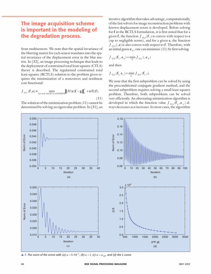
converges to a local minimizer. It is interesting to notethat the convergence analysis of this algorithm is still un-der investigation. The reconstructed image by regular-ized least squares (RLS) and the reconstructed image byRCTLS are shown in Figure 6(c) and (d), respectively.The reconstructed HR image using RCTLS shows im-provement both in image quality and PSNR.

In the proposed RCTLS algorithm, we find that thechoice of “proper” regularization parameterα is very im-portant. In Figure 7, we plot the norm of the error be-tween the real subpixel displacements and the estimatedsubpixel displacements by the algorithm for different val-ues of α. The speed of convergence decreases as α in-creases. In the case when α = −10 4 [Figure 7(a)] and α =1[Figure 7(b)], the norm of error after convergence isgreater than that in the first iteration. The “inappropri-ate” value of α makes the RCTLS solution fall into a localminimum. The L-curve method [17] may be used to getthe optimum value of the regularization parameter. TheL-curve method to estimate the “proper” α for RCTLS isused here. The L-curve plot is shown in Figure 7(d). Withα opt retrieved by L-curve, we see in Figure 7(c) that theRCTLS converges to a better minimum point (the normof error is significantly smaller than those obtained bychoosing α = −10 4 and α =1).

Color ImagesMultispectral restoration of a single image is a three-di-mensional (3-D) reconstruction problem where the thirdaxis incorporates different wavelengths. We are interestedin color images because there are many applications.Color image can be regarded as a set of three images intheir primary color channels (red, green, and blue).Monochrome processing algorithms applied to eachchannel independently are not optimal because they failto incorporate the spectral correlation between the chan-nels. Under the assumption that the spatial intrachanneland spectral interchannel correlationfunctions are product separable,Hunt and Kubler [20] showed that amultispectral (e.g., color) image canbe decorrelated by the Karhunen-Loeve transform (KLT). Afterdecorrelating multispectral images,the Wiener filter can be applied inde-pendently to each channel, and theinverse KLT gives the restored colorimage. It has recently been shown[33] that single color image restora-tion with multisensors can be formu-lated as a regularized least squaresproblem that can be solved efficientlyusing the fact that the DCT candiagonalize the linear system of equa-tions (resulting from the use ofNeumann boundary conditions),characterized by a BTHTHB matrix.

There is considerable scope for incorporatingregularization methods like the L-curve [7] in this ap-proach for further improvement in quality of restorationboth in the case of a single image as well as multispectralvideo sequences. In [34], Ng et al. also extended the HRimage reconstruction method to multiple undersampledcolor images. The key issue is to employ the cross-channelregularization matrix to capture the changes of reflectivityacross the channels.

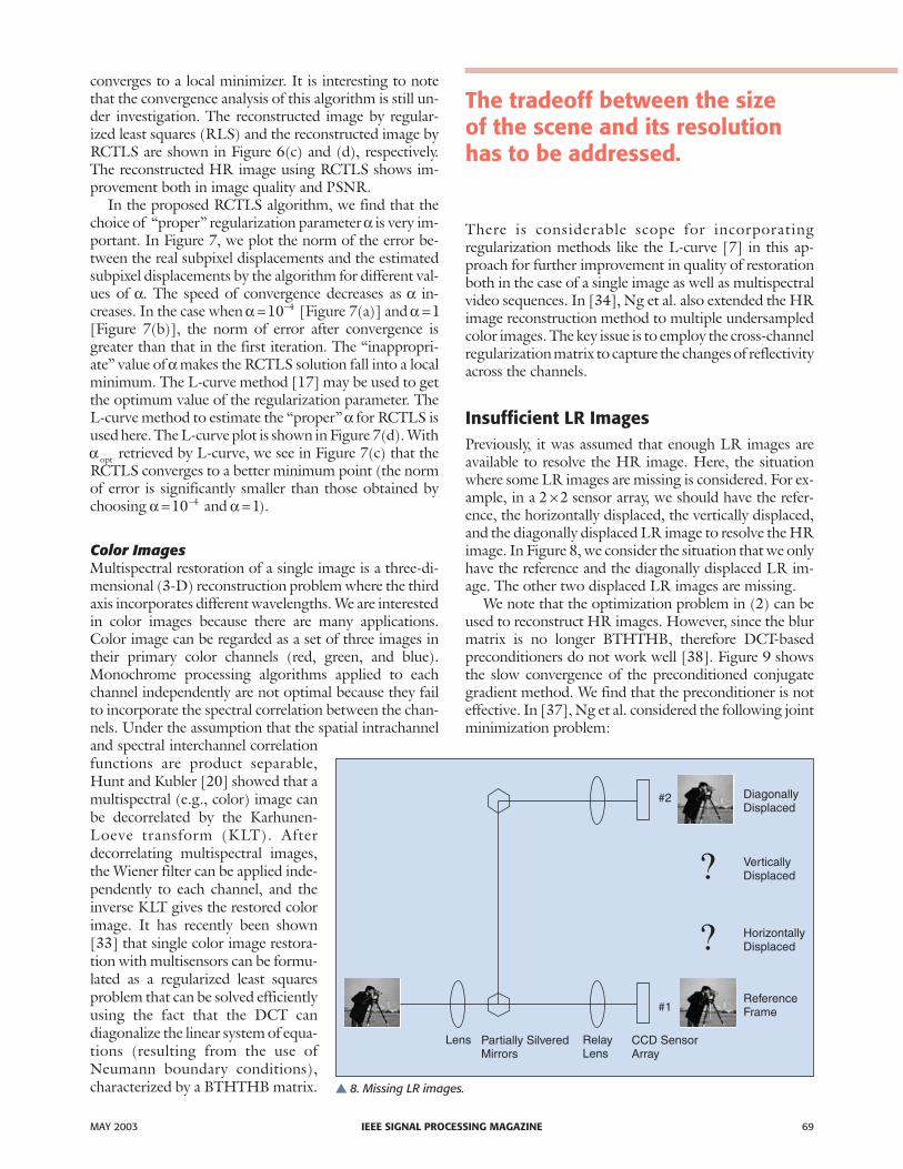
Insufficient LR ImagesPreviously, it was assumed that enough LR images areavailable to resolve the HR image. Here, the situationwhere some LR images are missing is considered. For ex-ample, in a 2 2× sensor array, we should have the refer-ence, the horizontally displaced, the vertically displaced,and the diagonally displaced LR image to resolve the HRimage. In Figure 8, we consider the situation that we onlyhave the reference and the diagonally displaced LR im-age. The other two displaced LR images are missing.

We note that the optimization problem in (2) can beused to reconstruct HR images. However, since the blurmatrix is no longer BTHTHB, therefore DCT-basedpreconditioners do not work well [38]. Figure 9 showsthe slow convergence of the preconditioned conjugategradient method. We find that the preconditioner is noteffective. In [37], Ng et al. considered the following jointminimization problem:

MAY 2003 IEEE SIGNAL PROCESSING MAGAZINE 69

#2

#1

DiagonallyDisplaced

VerticallyDisplaced

HorizontallyDisplaced

ReferenceFrame

Lens Partially SilveredMirrors

RelayLens

CCD SensorArray

� 8. Missing LR images.

The tradeoff between the sizeof the scene and its resolutionhas to be addressed.

min ( , ) min ( ) ( )

( ) ~(

, ,f f uf u e f u v

f u

u ILJ H≡ − +

+ +

12 2

2

1 2α α� � ) (12)

where u corresponds to the missing observed image pix-els because of the missing or faulty sensors in the sensorarray and u v+ and H are the full observed HR image anddegradation matrix, respectively, by combining all thesensors in the sensor array. Here � is the regularizationfunctional that was discussed earlier, and ~

� is the regular-ization functional for u, α1 and α 2 are positive parame-ters which measure the tradeoff between a good fit andthe regularity of the solutions f and u. Due to the local av-eraging of the pixel values in the image formation, the ob-served image pixel values are close to the neighbor imagepixel values. Our idea is to estimate u est , the missing ob-served image pixel u by using its neighbor image pixel val-ues v by, for instance, splines interpolation method [19].The regularization functional ~( )� u is defined to be

~( )� u u u≡ −12 2

2est .

Similarly, an alternating minimization algorithm is devel-oped for solving the joint minimization model (12).

Given u 0 : iterating k =1 2, ,K, until convergence

� Step i) Determine f f ufk IL kJ= −arg min ( , )1 by solving

the corresponding Euler-Lagrange equation:

( )H H R HTk

Tk( ) ( ) ( )( )e e f e u v+ = +−α1 1 .

� Step ii) Solve u f uuk kJ=arg min ( , ) by solving the cor-

responding Euler-Lagrange equation:

( ( )

( )

( )

1 21 2

1 2+ − −

× −

∈∑α )u

e f v

kl l s

l l

k

I D

H

missing sensor

− =α 2 0u est .

For Step i), the linear system can again be solved by thepreconditioned conjugate gradient method with the co-sine transform preconditioner. Therefore the linear sys-tem can be solved very efficiently. For Step ii), the vectoru k can be computed by using the matrix-vectormultiplication. Therefore the proposed algorithm for thejoint minimization model is more efficient than the directapplication of the cosine transform preconditioner formodel (2). Moreover, we see in Figures 10 and 11 that thequality of reconstructed images using the jointminimization model in (12) is better than those using themodel in (2).

The convergence of the above alternatingminimization algorithm can be analyzed by using theframework of fixed point theory. We just combine the twosteps of the alternating minimizing algorithm and derive

70 IEEE SIGNAL PROCESSING MAGAZINE MAY 2003

Rel

ativ

eR

esid

ual

Iterations

0 20 40 60 80 100 120 140 0 5 10 15 20 25 30

100

10−1

10−2

10−3

10−4

10−5

10−6

10−7

100

10−1

10−2

10−3

10−4

10−5

10−6

10−7

(a) (b)

� 9. Convergence behavior of the original system (- - -) and the cosine transform preconditioned system (—) when SNRs are (a) 50 dBand (b) 30 dB for missing two LR images.

Due to the ill-conditioning ofthe blurring matrix, theconvergence of iterative methodscan be very slow. How can wespeed up the convergence?

f e e ekT T

l l

H H R H=+

+

×

−

∈

11 2

11

1 2

αα[ ( ) ( ) ] ( )

( ) missing senso

[ ]rs

e

∑ −

+ +

×+

−

−

( ) ( )

( ) ( )

( )

I D H

H H R

H

l l k

T

T

1 2 1

1

1

2

21

e f

e e

e u

α

αα st +

+

1

1 2αv .

In [37], it has been shown that the spectral radius of thematrix

[ ]11 2

1

1

1 2

1 2

++

× −

−

∈

ααH H R

H I D

T

Tl l

l l

( ) ( )

( ) (( )

e e

emissing sensors∑ ) ( )H e

is less than one, and therefore the alternatingminimization algorithm converges globally to a mini-mizer for any given initial guess.

Edge-Preserving RegularizationThe H1 -norm regularization tends to attenuate the highfrequency information of the HR image. Therefore,

MAY 2003 IEEE SIGNAL PROCESSING MAGAZINE 71

(a) (b) (c)

� 10. (a) Original and (b), (c) two LR images.

(a) (b) (c)

� 11. Reconstructed images using (a) the model in (2) [relative error = 0.0614], (b) the joint minimization model with the H 1-norm reg-ularization [relative error = 0.0574], and (c) the joint minimization model with the total variation regularization [relative error =0.0931].

If we consider edge-preservingregularization models,can we design an efficientiterative method for solvingthe correspondingminimization problem?

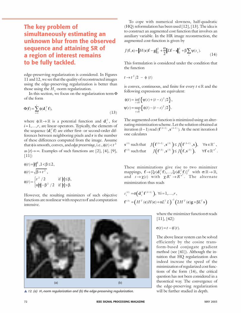
edge-preserving regularization is considered. In Figures11 and 12, we see that the quality of reconstructed imagesusing the edge-preserving regularization is better thanthose using the H1 -norm regularization.

In this section, we focus on the regularization term Φof the form

Φ( ) ( )f d f==∑φi

r

iT

1

,(13)

where φ:� �→ is a potential function and d iT , for

i r=1, ,K , are linear operators. Typically, the elements ofthe sequence { }d fi

T are either first- or second-order dif-ferences between neighboring pixels and r is the numberof these differences computed from the image. Assumethat φ is smooth, convex, and edge preserving, i.e., φ( )t t< 2

as| |t → ∞. Examples of such functions are [2], [4], [9],[11]:

φ = < ≤

φ = +

φ =≤

− >

( ) , ,

( ) ,

( )/ ,

/

t t

t t

tt

β β

β

βα τ β

1 2

22

2

2

2

if tif t β.

However, the resulting minimizers of such objectivefunctions are nonlinear with respect to f and computationintensive.

To cope with numerical slowness, half-quadratic(HQ) reformulation has been used [12], [13]. The idea isto construct an augmented cost function that involves anauxiliary variable. In the HR image reconstruction, theaugmented cost-function is given by

J H L si

i( , ) ( ) ( )f s e f g f s= − + − + ∑2

2

2

2

2α β ψ .

(14)

This formulation is considered under the condition thatthe function

t t t→ −2 2/ ( )φ

is convex, continuous, and finite for every t ∈� and thefollowing expressions are equivalent:

{ }{ }

φ ψ

ψ φ

( ) inf ( ) ( ) / ,

( ) ( ) ( ) / .

t s t s

s t t ss R

t R

= + −

= − −∈

∈

2

2

2

2sup

The augmented cost function is minimized using an alter-nating minimization scheme. Let the solution obtained atiteration ( )k −1 read ( , )( ) ( )f sk k− −1 1 . At the next iteration kone calculates

( ) ( )s f s f s s

f

( ) ( ) ( ) ( )

( )

, , , ,k k k k r

k

J Jsuch that

such t

− −≤ ∀ ∈1 1�

( ) ( )hat J Jk k k nf s f s f( ) ( ) ( ), , , .≤ ∀ ∈�2

These minimizations give rise to two minimizermappings, f d f d f→ [ ( ), , ( )]ξ ξs sT

rT T

1 K with σ:� �→ ,and s s→ χ( ) with χ:R Rr n→

2

. The alternateminimization thus reads

( )( )

s i r

H H L L H

ik

iT k

k T T T

( ) ( )

( )

, , , ,

( ) ( )

= ∀ =

= +

−

−

σ

α

d f

f e e

1

1

1

2

K

( )( )e g s+ βLT

where the minimizer functionσ reads[11], [42]:

σ φ( ) '( )t t t= − .

The above linear system can be solvedefficiently by the cosine trans-form-based conjugate gradientmethod (see [41]). Although the in-tuition that HQ regularization doesindeed increase the speed of theminimization of regularized cost func-tions of the form (14), the criticalquestion has not been considered in atheoretical way. The convergence ofthe edge-preserving regularizationwill be further studied in depth.

72 IEEE SIGNAL PROCESSING MAGAZINE MAY 2003

(a) (b)

� 12. (a) H1-norm regularization and (b) the edge-preserving regularization.

The key problem ofsimultaneously estimating anunknown blur from the observedsequence and attaining SR ofa region of interest remainsto be fully tackled.

Future ResearchIt is usually not possible at the outset to achieve the de-sired resolution because of technology and cost con-straints. For example, the technology of a CCD islimited by factors like physical dimension, shot noise,and parasitic effects. In applications like astronomicalimaging, the reduced size and weight of cameras in aspaceship or satellite affect its quality. The need fortradeoff between size, weight, and quality of the CCDarray necessitates the design of SR algorithms to obtainthe desired HR image of a common region of interest inthe frames of a video sequence without modifying thephysical characteristics of the CCD array. Imperfect op-tics, finite detector arrays, and finite individual detectorsizes all contribute to a variety of degradation processesto which an image acquisition system is susceptible.Dramatic progress has been documented during the lastdecade in the area of HR image processing that encom-passes the stages of image registration or camera motionparameter estimation, deblurring, noise reduction (fil-tering), and interpolation.

Considerable research activity is being witnessed inareas pertaining to the construction of a panoramic mo-saic followed by the attainment of spatial resolution in-crease of regions of interest in the mosaic. In video, theuser gets the sequence of images containing both spatialand temporal information. The number of pixels in eachframe is fixed to a known resolution. To generate one bigsnapshot of the scene that covers all desired areas (pan-oramic mosaic), one needs to adjust the camera in vari-ous ways to capture the effects of zooming, panning,tilting, etc., that may be required for capturing the entirescene. Usually, the resulting picture will suffer fromundersampling or LR effect because the whole scene hasto be represented by the limited number of pixels. There-fore, the bigger the scene, the lower will be the resolu-tion. On the other hand, higher resolution of regions ofinterest in the scene can be obtained if the camera iszoomed to those specific regions. Therefore the tradeoffbetween the size of the scene and its resolution has to beaddressed. In the future, more research is needed on howto take advantage of the intraframe spatial informationalong with interframe temporal information to createthe HR panoramic image and then attain SR of regionsof interest in the mosaic.

The key problem of simultaneously estimating an un-known blur from the observed sequence and attainingSR of a region of interest remains to be fully tackled.Blind deconvolution refers to the problem of restoringthe original image from a degraded observation and in-complete blur informat ion. Exis t ing bl inddeconvolution techniques can be categorized into twomain classes. One approach treats blur identification andimage super resolution separately. The other approachimplements the two subtasks simultaneously. Both ap-proaches are adaptable from the single image case to themultiframe situation of interest here. Initial results in

this area of blind robust super resolution have beenreported recently [26]. Recently, Nguyen et al. [40] con-sidered the blind deconvolution problem in themultiframe case. Their algorithm can handle only thePSF, which is modeled by one parameter. This restric-tion is very limited in many applications.

AcknowledgmentsThis research was supported in part by RGC GrantsHKU 7132/00P and 7130/02P and by Army ResearchOffice Grant DAAD 19-00-1-0539.

Michael K. Ng received the B.Sc. and M.Phil. degrees inmathematics from the University of Hong Kong in 1990and 1993, respectively, and the Ph.D. degree in mathe-matics from the Chinese University of Hong Kong, in1995. From 1995 to 1997 he was a research fellow at theAustralian National University, Canberra. He is currentlyan associate professor in the Department of Mathematicsat the University of Hong Kong. His research interestsare in the areas of data mining, operations research, andscientific computing. He was one of the recipients of theOutstanding Young Researcher Award of the Universityof Hong Kong in 2001.

Nirmal K. Bose received the B. Tech (Hons.), M.S., andPh.D. degrees in electrical engineering from I.I.T.,Kharagpur, India, Cornell University, and Syracuse Uni-versity, respectively. He was a professor of electrical engi-neering and of mathematics at the University ofPittsburgh. He joined Pennsylvania State University,University Park, in 1986 as Singer Professor and in 1992was named the HRB-Systems Professor of electrical engi-neering. He is the author of several recognized texts andsince is the founding editor-in-chief of the InternationalJournal on Multidimensional Systems and Signal Processing.He has served as visiting faculty at several institutions, in-cluding the American University of Beirut, Lebanon, andPrinceton University, New Jersey. He is a Fellow of theIEEE. His most recent honors include the InvitationalFellowship from the Japan Society for the Promotion ofScience in 1999, the Alexander von Humboldt ResearchAward from Germany in 2000, and the Charles H. FetterUniversity Endowed Fellowship in Electrical Engineer-ing from 2001-2004.

References[1] H. Andrew and B. Hunt, Digital Image Restoration. Englewood Cliffs, NJ:

Prentice-Hall, 1977.

[2] G. Aubert and L. Vese, “A variational method in image recovery,” SIAM J.Numer. Anal., vol. 34, pp. 1948-1979, 1997.

[3] M. Banham and A. Katsaggelos, “Digital image restoration,” IEEE SignalProcessing Mag.,vol. 14, pp. 24-41, Mar. 1997.

[4] M. Black and A. Rangarajan, “On the unification of line processes, outlierrejection, and robust statistics with applications to early vision,” Int. J.Comput. Vision, vol. 19, pp. 57-91, 1996.

MAY 2003 IEEE SIGNAL PROCESSING MAGAZINE 73

[5] K. Boo and N.K. Bose, “Two-dimensional model-based power spectrumestimation for nonextendible correlation bisequences,” Circuits Syst. SignalProcess., vol. 16, no. 2, pp. 141-163, 1997.

[6] N.K. Bose and K. Boo, “Asymptotic eigenvalue distribution ofblock-Toeplitz matrices,” IEEE Trans. Inform. Theory, vol. 44, no. 2, pp.858-861, 1998.

[7] N.K. Bose, S. Lertrattanapanich, and J. Koo, “Advances in superresolutionusing the L-curve,” in Proc. Int. Symp. Circuits and Systems, Sydney, Austra-lia, May 2001, pp. 433-436.

[8] N.K. Bose and K. Boo, “High-resolution image reconstruction withmultisensors,” Int. J. Imaging Syst. Technol., vol. 9, pp. 294-304, 1998.

[9] C. Bouman and K. Sauer, “A generalized Gaussian image model foredge-preserving MAP estimation,” IEEE Trans. Image Processing, vol. 2, pp.296-310, July 1993.

[10] R. Chan, T. Chan, M. Ng, W. Tang, and C. Wong, “Preconditioned itera-tive methods for high-resolution image reconstruction with multisensors,”in Proc. SPIE Symp. Advanced Signal Processing: Algorithms, Architectures, andImplementations, vol. 3461, San Diego, CA, July, 1998, pp. 348-357.

[11] P. Charbonnier, L. Blanc-Feraud, G. Aubert, and M. Barlaud, “Determin-istic edge-preserving regularization in computer imaging,” IEEE Trans. Im-age Processing, vol. 6, pp. 298-311, Feb. 1997.

[12] D. Geman and G. Reynolds, “Constrained restoration and recovery of dis-continuities,” IEEE Trans. Pattern Anal. Machine Intell., vol. 14, pp.367-383, Mar. 1992.

[13] D. Geman and C. Yang, “Nonlinear image recovery with half-quadraticregularization,” IEEE Trans. Image Processing, vol. 4, pp. 932-946, July1995.

[14] J. Gillete, T. Stadtmiller, and R. Hardie, “Aliasing reduction in staring in-frared images using subpixel techniques,” Opt. Eng., vol. 34, pp.3130-3137, Nov. 1995.

[15] G. Golub and C. Van Loan, Matrix Computations, 2nd ed. Baltimore,MD: Johns Hopkins Univ. Press, 1989.

[16] R. Gonzalez and R. Woods, Digital Image Processing. New York: AddisonWesley, 1992.

[17] P. Hansen and D. O’Leary, “The use of the L-curve in the regularzationof discrete ill-posed problems,” SIAM J. Sci. Comput., vol. 14, pp.1487-1503, 1993.

[18] M. Hestenes and E. Steifel, “Methods of conjugate gradient for solvinglinear systems,” J. Res. Nat. Bureau Stand., vol. 49, pp. 409-436, 1952.

[19] H. Hou and H. Andrews, “Cubic splines for image interpolation and di-agonal filtering,” IEEE Trans. Accoust Speech Signal Processing, vol. 26, pp.508-517, Dec. 1978.

[20] B. Hunt and O. Kubler, “Karhunen-Loeve multispectral image restora-tion, part I: Theory,” IEEE Trans. Acoust., Speech, Signal Processing, vol. 32,pp. 592-600, June 1984.

[21] G. Jacquemod, C. Odet, and R. Goutte, “Image resolution enhancementusing subpixel camera displacement,” Signal Processing, vol. 26, pp.139-146, 1992.

[22] T. Komatsu, K. Aizawa, T. Igarashi, and T. Saito, “Signal-processingbased method for acquiring very high resolution images with multiple cam-eras and its theoretical analysis,” Proc. Inst. Elec. Eng. vol. 140, no. 3, pt. I,pp. 19-25, 1993.

[23] J. Koo and N.K. Bose, “Spatial restoration with reduced boundary error,”in Proc. Mathematical Theory of Networks and Systems (MTNS), Univ. of No-tre Dame, South Bend, IN., Aug. 12-16, 2002 [Online]. Available:http://www.ndu.edu/~mtns/talksalph.html

[24] R. Lagendijk and J. Biemond, Iterative Identification and Restoration of Im-ages. Norwell, MA: Kluwer, 1991.

[25] S. Lertrattanapanich and N.K. Bose, “Latest results on high-resolution re-construction from video sequences,” Inst. Electronic, Information andCommunication Eng., Japan, Tech. Rep. IEICE, DSP99-140, Dec. 1999,pp. 59-65.

[26] S. Lertrattanapanich and N.K. Bose, “High resolution image formationfrom low resolution frames using Delaunay triangulation,” IEEE Trans. Im-age Processing, vol. 11, no. 12, pp. 1427-1441, Dec. 2002.

[27] D. Luenberger, Linear and Nonlinear Programming, 2nd ed. Reading,MA: Addison-Wesley,1984.

[28] F. Luk and D. Vandevoorde, “Reducing boundary distortion in imagerestoration,” in Proc. SPIE 2296, Advanced Signal Processing Algorithms, Ar-chitectures and Implementations VI, 1994, pp. 554-565.

[29] S. Mann and R. Picard, “Video Orbits of the projective group: A simpleapproach to featureless estimation of parameters,” IEEE Trans. Image Pro-cessing, vol. 6, pp. 1281-1295, Sept. 1997.

[30] M. Ng, “An efficient parallel algorithm for high-resolution color image re-construction,” Proc. the Seventh Int. Conf. Parallel and Distributed Systems:Workshops, Iwate, Japan, 4-7 July, 2000, pp. 547-552,

[31] M. Ng, N.K. Bose, and J. Koo, “Constrained total least squares computa-tions for high resolution image reconstruction with multisensors,” Int. J.Imaging Syst. Technol., vol. 12, pp. 35-42, 2000.

[32] M. Ng and N.K. Bose, “Analysis of displacement errors in high-resolutionimage reconstruction with multisensors,” IEEE Trans. Circuits Syst. I, vol.49, pp. 806-813, June 2002.

[33] M. Ng and N.K. Bose, “Fast color image restoration with multisensors,”Int. J. Imaging Syst. Technol., to be published.

[34] M. Ng, N.K. Bose, and J. Koo, “Constrained total least squares for colorimage reconstruction,” in Total Least Squares and Errors-in-Variables Model-ling III: Analysis, Algorithms and Applications, S. Huffel and P. Lemmerling,Eds. Norwell, MA: Kluwer, 2002, pp. 365-374.

[35] M. Ng, R. Chan, and W. Tang, “A fast algorithm for deblurring modelswith Neumann boundary conditions,” SIAM J. Sci. Comput., vol. 21, pp.851-866, 1999.

[36] M. Ng, R. Chan, T. Chan, and A. Yip, “Cosine transform preconditionersfor high resolution image reconstruction,” Linear Algebra Applicat., vol.316, pp. 89-104, 2000.

[37] M. Ng, W. Ching, K. Sze, and A. Yau, “Super-resolution image recon-struction using multisensors,” Numerical Linear Algebra with Applications, tobe published.

[38] M. Ng and K. Sze, “Preconditioned iterative methods for superresolutionimage reconstruction with multisensors,” SPIE, Symp. Advanced Signal Pro-cessing: Algorithms, Architectures and Implementations, vol. 4116, San DiegoCA, 2000, pp. 396-405.

[39] M. Ng and A. Yip, “A fast MAP algorithm for high-resolution image re-construction with multisensors,” Multidimensional Syst. Signal Process., vol.12, no. 2, pp. 143-164, 2001.

[40] N. Nguyen, P. Milanfar, and G. Golub, “Efficient generalized cross-valida-tion with applications to parametric image restoratioin and resolution en-hancement,” IEEE Trans. Image Processing, vol. 10, pp. 1299-1308, Sept.2001.

[41] M. Nikolova and M. Ng, “Fast image reconstruction algorithms combin-ing half-quadratic regularization and preconditioning,” in Proc. IEEE Int.Conf. Image Processing, 2001, vol. I, pp. 277-280.

[42] M. Nikolova and M. Ng, “Comparison of the main forms of half-qua-dratic regularization,” in Proc. IEEE Int. Conf. Image Processing, Rochester,NY, Sept. 2002, vol. I, pp. 349-352.

[43] S. Van Huffel and J. Vandewalle, The Total Least Squares Problem: Compu-tational Aspects and Analysis. Philadelphia, PA: SIAM, 1991.

74 IEEE SIGNAL PROCESSING MAGAZINE MAY 2003