TITLE: Generative Representations for the Automated Design of Modular Physical Robots

Gregory S. Hornby1, Hod Lipson2, Jordan B. Pollack

Computer Science Dept, Brandeis University, Waltham, MA 02454 USA

Contact author: Hod Lipson (IEEE Member) Mechanical & Aerospace Engineering Cornell University, 216 Upson Hall, Ithaca NY 14853, USA Office: (607) 255 1686 Fax: 255 1222 Email: Hod.Lipson@cornell.edu http://www.mae.cornell.edu/lipson Gregory S. Hornby Computational Sciences Division, NASA Ames Research Center, Moffett field, CA, USA Email: hornby@email.arc.nasa.gov Jordan B. Pollack Computer Science Department Center for Complex Systems Brandeis University (781) 736-2713 pollack@cs.brandeis.edu KEYWORD: Evolutionary robotics, design automation, generative representations The material in this paper was partially presented at the IEEE Conference on robotics and Automation, ICRA 2001

1 Current address: Computational Sciences Division, NASA Ames Research Center, Moffett field, CA, USA 2 Current address: Mechanical & Aerospace Engineering, Cornell University, Ithaca NY, USA

2

ABSTRACT

The field of evolutionary robotics has demonstrated the ability to automatically design the

morphology and controller of simple physical robots through synthetic evolutionary

processes. However, it is not clear if variation-based search processes can attain the

complexity of design necessary for practical engineering of robots. Here we demonstrate an

automatic design system that produces complex robots by exploiting the principles of

regularity, modularity, hierarchy and reuse. These techniques are already established

principles of scaling in engineering design and have been observed in nature, but have not

been broadly used in artificial evolution. We gain these advantages through the use of a

generative representation, which combines a programmatic representation with an

algorithmic process that compiles the representation into a detailed construction plan. This

approach is shown to have two benefits: (a) it can reuse components in regular and

hierarchical ways, providing a systematic way to create more complex modules from

simpler ones, and (b) the evolved representations can capture intrinsic properties of the

design space, so that variations in the representations move through the design space more

effectively than equivalent sized changes in a non-generative representation. Using this

system we demonstrate for the first time the evolution and construction of modular, three-

dimensional, physically locomoting robots, comprising many more components than

previous work on body-brain evolution.

3

Introduction

The field of evolutionary robotics has demonstrated the ability to automatically design both the

morphology and controller of simple physical robots through synthetic evolutionary processes (e.g.

Sims, 1994; Nolfi and Floreano, 2000; Lipson and Pollack, 2000). Despite these results, it is not

clear if these genetically inspired search algorithms can attain the design complexity necessary for

practical engineering. The ultimate success of these methods as tools for design automation is

critically dependent on the scaling properties of the representations. Representations in which each

element of the encoded design are used at most once in translating to the design (non-generative

representations) scale linearly with the number of parts in the artifact. Consequently, search

algorithms that use this style of representation will quickly become exponentially intractable, and

thus will not scale to complex tasks.

In this paper we seek ways to circumvent this fundamental restriction with the automated design of

robots by using a generative representation for encoding each robot. A robot is defined by a

compact programmatic form (its generative representation) and the evolutionary variation takes

place on this form. Evaluation requires the representation to be compiled into a detailed

construction plan for manufacturing the robot in simulation or reality Thus, the generative

representations are varied through the evolutionary search process, while the evaluation or fitness

function is applied to the construction plans.

Compared to previous work in evolutionary robotics, generative representations demonstrate two

advantages. First, a generative representation allows for the reuse of components in regular and

hierarchical ways, providing a systematic way to create more complex modules out of simpler ones.

We show this through our evolved designs. Second, the evolved generative representation may

itself capture intrinsic properties of the design problem, so that variations in the representations

move through the design space very effectively. We demonstrate this by showing that across many

generations of machines, mutations on the generative representation, despite causing larger-scale

changes, are more productive than mutations on a non-generative representation. Both of these

aspects maintain the evolvability of the design while its complexity rises.

In this paper we bring together ideas of automated design and generative representations, and apply

them to the design of physical working robots for a limited physical domain. Although the robots

4

we have built from this process are still very simple compared to human-engineered machines, their

structure is more principled (regular, modular and hierarchical) compared to previously evolved

machines of comparable functionality, and the virtual designs which are achieved by the system

have an order of magnitude more moving parts. Moreover, we quantitatively demonstrate for this

design space how the generative representation is capable of searching more efficiently than a non-

generative representation.

Structure of this paper

We will begin with a brief background of evolutionary robotics and related work, and demonstrate

the scaling problem with our own prior results. Next we propose the use of an evolved generative

representation as opposed to a non-generative representation. We describe this representation in

detail as well as the evolutionary process that uses it. We then compare progress of evolved robots

with and without the use of the grammar, and quantify the obtained advantage. Working two-

dimensional and three-dimensional physical robots produced by the system are shown.

Background

Biological evolution is characterized as a process applied to a population of individuals, which are

subject to selective replication with variation (Maynard-Smith and Szathmary, 1995). Evolutionary

design systems use the same principles of biological evolution to achieve machine design, yet add a

target to the evolution – the functional requirements specified by the designer. Candidate designs in

a population are thus still selected, replicated and varied, but selection is governed by an external

design criteria. After a number of generations the selective evolutionary process may breed an

acceptable design.

Genetic algorithms – a subset of evolutionary computation involving mutation and crossover in a

population of fixed length bit strings (Holland, 1975) – have been applied for several decades in

many engineering problems as an optimization technique for a fixed set of parameters.

Alternatively, more recent open-ended evolutionary design systems, in which the process is

allowed to add more and more building blocks and parameters, seem particularly adequate to

design problems requiring synthesis. Such open-ended evolutionary design systems have been

demonstrated for a variety of simple design problems, including structures, mechanisms, software,

optics, robotics, control, and many others (for overviews see, for example, Koza, 1992; Bentley,

5

1999; Husbands et al, 1998). Yet these accomplishments remain simple compared to what teams of

human engineers can design and what nature has produced. The evolutionary design approach is

often criticized as scaling badly when challenged with design requirements of higher complexity.

(Mataric and Cliff, 1996)

While there are still many poorly understood factors that determine the success of evolutionary

design – such as starting conditions, variation operators, primitive building blocks and fidelity of

simulation – one problem is that the design space is exponentially large, because there is an

exponentially increasing number of ways a linearly increasing set of components can be assembled.

Consequently, evolutionary approaches that operate on non-generative representations quickly

become intractable.

Indeed, while our own experiments in open-ended evolutionary design of mechanisms and

controllers for locomotion (Lipson and Pollack, 2000) have produced physically viable

mechanisms, the design progress appears to eventually reach a plateau. Figures 1a and Figure 1b

show the progress of a typical run. The abscissa represents evolutionary time (generations), the

ordinate measures fitness (net movement on a horizontal plane) and each point in the scatter plot

represents one candidate robot. In general, after an initial period of drift, with zero fitness, we

observe rapid growth followed by a logarithmic slowdown in progress3, characterized by longer

and longer durations4 between successive step-improvements in the fitness. We thus hypothesize

that one of the primary challenges in evolutionary robotics research is that of allowing the process

to identify and reuse assemblies of parts, creating more complex components from simpler ones.

This reuse would, in turn, lead to acceleration in the discovery process, leading in turn to higher

level of search, and so forth. This scaling in knowledge and unit of construction – hierarchical

modularity – is observable in the engineering (.e. Ulrich and Tung, 1991; Huang and Kusiak,

1998), economic organization (Langlois, 2001) and in nature (e.g. Hartwell et al, 1999).

Theoretical analysis reveals that allowing an evolutionary process to repeatedly aggregate low-level

3 However, note that because of the stochastic nature of the process, it is hard to determine definitely whether

progress has actually halted, and improvements may still occur after long periods of apparent stagnation (Figures 1c

and 1d). 4 This real time lingering is amplified by the fact that evaluation time or duration of a generation (in simulation or

in physical reality) also increases as solutions become more complex

6

building blocks into higher-level groups in a hierarchical fashion, potentially transforms the design

problem from exponential complexity to polynomial complexity under certain conditions (Watson

and Pollack, 2001). The challenge then becomes the continuous identification of discovered

components and the encapsulation of them as basic units of change in the variation operators. In

other words, the design space in which the machines are specified and the effects of mutations and

crossovers which move through the space need to evolve over time as well.

Generative representations

Generative representations (Hornby and Pollack 2001) are a class of representations in which

elements in the encoded data structure of a design can be reused in creating the design.

Implemented as a kind of a computer program, a generative representation can allow the definition

of reusable sub-procedures that can be activated in loops and recursive calls, allowing the design

system to scale to more complex tasks, in fewer steps, than can be achieved with a non-generative

representation. Examples of representations that are generative are genetic programming with

automatically defined functions (Koza, 92) and cellular encoding (Gruau, 94), which has

procedures and loops.

Here we use Lindenmayer systems (L-systems) as the generative representation for robot designs.

L-systems are a grammatical rewriting system introduced to model the biological development of

multicellular organisms (Lindenmayer, 1968). Rules are applied in parallel to all characters in the

string, just as cell divisions happen in parallel in multicellular organisms. Complex objects are

created by successively replacing parts of a simple object by using the set of rewriting rules. A

detailed specification of the L-system used in this work follows in the next section.

L-systems and evolutionary algorithms have been used both on their own and together to create

designs. L-systems have been used mainly to construct tree-like plants, (Prusinkiewicz and

Lindenmayer, 1990). However, it is difficult to manually design an L-system to produce a desired

form. L-systems have been combined with evolutionary algorithms in previous work, such as the

evolution of plant-like structures (Prusinkiewicz and Lindenmayer, 1990; Jacob, 1994; Ochoa,

1998) and architectural floor designs (Coates, 1999), but only limited results have been achieved,

and none have resulted in dynamic physical machines comprising any form of control.

7

Robot morphology and controllers have been automatically designed both separately and

concurrently. Genetic algorithms have been used to evolve a variety of different control

architectures for a fixed morphology, such as: stimulus-response rules (Ngo and Marks, 1993);

neural controllers (Grzeszczuk 1995); and gait parameters (Hornby et al, 1999). Again using

genetic algorithms, serial manipulators have been evolved by evaluating the ability of their end

manipulator to achieve a set of configurations (Kim and Khosla, 1993; Chen and Burdick, 1995;

Paredis, 1996; and Chocron and Bidaud, 1997); and tree-structured robots have been evolved that

met a set of requirements on static stability, power consumption and geometry (Farritor et al, 1996;

Farritor and Dubowsky, 2001). Leger’s Darwin2K (1999) uses fixed control algorithms to evaluate

evolved robot morphologies. Unlike the previous systems, which did not allow for reuse or the

hierarchical construction of modules, Darwin2K has a kind of abstraction that allows the same

assembly of parts to be reused. But the ability to design controllers is necessary for evaluating

robots for more complex tasks or in dynamic environments (Roston, 1994; Pollack et al, 2000).

Concurrent development of robot morphology and controllers has been achieved previously by

Sims (1994), Komosinski and Rotaru-Varga (2000) and ourselves (Lipson and Pollack, 2000), all

of which used evolutionary algorithms to simultaneously create the morphology and a neural

controller in simulation. Whereas Sims and Komosinski et al were not concerned with the

feasibility of their creations in reality, the focus of our own line of work is to show that robots

created through evolution in simulation could be successfully transferred to reality. This work

extends our initial results by investigating generative representations as a mechanism to overcome

the complexity barrier.

Method

We used four levels of computation, as follows:

1. An evolutionary process that evolves generative representations of robots.

2. Each generative representation is an L-System program that, when compiled, produces a

sequence of build commands, called an assembly procedure.

3. A constructor executes an assembly procedure to generate a robot (both morphology and

control).

8

4. A physical simulator tests a specific robots’ performance according to a fitness criteria, to

yield a figure of merit that is fed back into the evolutionary process (1).

We will describe each of the above four levels.

Constructor and design language

The design constructor builds a model from a sequence of build commands. The language of build

commands is based upon instructions to a LOGO-style turtle, which direct it to move forward,

backward or rotate about a coordinate axis. The commands are listed in Table I. Robots (called

“Genobots”, for generatively encoded robots) are constructed from rods and joints,

Figure 2, that are placed along the turtle’s path. Actuated joints are created by commands that direct

the turtle to move forward and place an actuated joint at its new location, with oscillatory motion

and a given offset.

The operators “[“ and “]” push and pop the current state – consisting of the current rod, current

orientation, and current joint oscillation offset – to and from a stack. Forward moves the turtle

forward in the current direction, creating a rod if none exists or traversing to the end of the existing

rod. Backward goes back up the parent of the current rod. The rotation commands turn the turtle

about the Z-axis in steps of 60°, for 2D robots, and about the X, Y or Z axes, in steps of 90°, for 3D

robot. Joint commands move the turtle forward, creating a rod, and end with an actuated joint. The

parameter to these commands specify the speed at which the joint oscillates, using integer values

from 0 to 5, and the relative phase-offset of the oscillation cycle is taken from the turtle’s state.

The commands “Increase-offset” and “decrease-offset” change the offset value n the turtle's state

by ±25% of a total cycle. Command sequences enclosed by “{ }” are repeated a number of times

specified by the brackets' argument.

For example, the string,

{ joint(1) [ joint(1) forward(1) ] clockwise(2)}(3)

is interpreted as:

{joint(1) [ joint(1) forward(1) ] clockwise(2)

joint(1) [ joint(1) forward(1) ] clockwise(2)

9

joint(1) [ joint(1) forward(1) ] clockwise(2)}

and produces the robot in .

Constructed robots do not have a central controller; rather each joint oscillates independent of the

others. More recent work has integrated a recurrent neural network as the robot controller (Hornby

and Pollack, in press). In the figures, large crosses (×’s) are used to show the location of actuated

joints and small crosses show unactuated joints. The left image shows the robot with all actuated

joints in their starting orientation and the image on the right shows the same robot with all actuated

joints at the other extreme of their actuation cycle. In this example all actuated joints are moving in

phase.

Parametric OL-Systems

The class of L-systems used as the representation is a parametric, context-free L-system (P0L-

system). Formally, a P0L-system is defined as an ordered quadruplet, G = (V, Σ, ω, P) where,

V is the alphabet of the system,

Σ is the set of formal parameters,

ω ∈ (V × ℜ*)+ is a nonempty parametric word called the axiom, and

P ⊂ (V × Σ*) × C(Σ) × (V × ξ(Σ))* is a finite set of productions.

The symbols “:” and “à” are used to separate the three components of a production: the

predecessor, the condition and the successor. For example, a production with predecessor A(n0,n1),

condition n1>5 and successor B(n1+1)cD(n1+0.5, n0-2) is written as:

A(n0, n1): n1 > 5 à B(n1+1)cD(n1+0.5, n0-2)

A production matches a module in a parametric word if and only if the letter in the module and the

letter in the production predecessor are the same, the number of actual parameters in the module is

equal to the number of formal parameters in the production predecessor, and the condition

evaluates to true if the actual parameter values are substituted for the formal parameters in the

production.

10

For ease of implementation we add constraints to our P0L-system. The condition is restricted to be

comparisons as to whether a production parameter is greater than a constant value. Parameters to

design commands are either a constant value or a production parameter.

Parameters to productions are equations of the form:

[production parameter | constant ] [+ | – | × | \ ] [production parameter | constant ]

The following is a P0L-system using the language defined in Table I and consists of two

productions with each production containing two condition-successor pairs:

P0(n): n > 2 à {P0(n – 1) }(n)

n > 0 à joint(1) P1(n × 2) clockwise(2)

P1(n): n > 2 à [ P1(n / 4) ]

n > 0 à joint(1) forward(1)

If the P0L-system is started with P0(3), the resulting sequence of strings is produced:

P0(3)

{ P0(2) }(3)

{ joint(1) P1(4) clockwise(2) }(3)

{ joint(1) [ P1(1) ] clockwise(2) }(3)

{ joint(1) [ joint(1) forward(1) ] clockwise(2) }(3)

This produces the robot in .

The evolutionary process

An evolutionary algorithm is used to evolve individual L-systems. Evolutionary algorithms are a

stochastic search and optimization technique inspired by natural evolution (Holland, 1975; Back et

al, 1991). An evolutionary algorithm maintains a population of candidate solutions from which it

performs search by iteratively replacing poor members of the population with individuals generated

by applying variation to good members of the population. The initial population of L-systems is

11

created by making random production rules. Evolution then proceeds by iteratively selecting a

collection of individuals with high fitness for parents and using them to create a new population of

individual L-systems through mutation and recombination. Since the initialization process and the

variation operators are customized for our representation we discuss them in greater detail.

Mutation creates a new individual by copying the parent individual and making a small change to

it. Changes that can occur are: replacing one command with another; perturbing the parameter to a

command by adding/subtracting a small value to it; changing the parameter equation to a

production; adding/deleting a sequence of commands in a successor; or changing the condition

equation.

Recombination takes two individuals, p1 and p2, as parents and creates one child individual, c, by

making it a copy of p1 and then inserting a small part of p2 into it. This is done by replacing one

successor of c with a successor of p2, inserting a sub-sequence of commands from a successor in p2

into c, or replacing a sub-sequence of commands in a successor of c within a sub-sequence of

commands from a successor in p2. Details of the mutation and recombination operators used here,

as well as other evolutionary algorithm parameters, are described in an earlier report (Hornby and

Pollack 2000).

Since we were trying to evolve machines that could locomote, fitness was defined as the distance

moved by the robot's center of mass after 10 simulated oscillation cycles. This distance is

normalized by one tenth of the length of a basic bar, to produce a dimensionless figure.

The evolutionary algorithm described in the methods section of this paper is essentially a canonical

evolutionary algorithm, differing only in the representation. First, a population size of one hundred

individuals is used and this is run for five hundred generations. Once individuals are evaluated,

their fitness score is adjusted to a probability of reproducing using exponential scaling with a

scaling factor of 0.03 (Michalewicz, 92). Individuals are then selected as parents using stochastic

remainder selection (Back, 96). New individuals are created through applying mutation or

recombination (chosen with equal probability) to individuals selected as parents. The two best

individuals from each generation were copied directly to the next generation without mutation or

crossover (elitism of 2). Since the initialization process, mutation operator and recombination

operator are all tightly coupled to the representation we describe each of these parts in greater

detail.

12

Initializing the population consists of creating a set of random L-systems. A random L-system has

a fixed number of production rules, with each having the same number of condition successor pairs,

so creating a new individual consists of creating a number of random conditions and successors. A

new condition is created by selecting a random parameter and a random value to compare against.

New successors are created by stringing together sequences of one to three construction symbols,

with each sequence being enclosed with push/pop brackets, block replication parenthesis, or

neither. Examples of these blocks of commands are:

Forward(n0) left(4.0)

{ up(1.0) }(2.0)

[ back(2.0) down(1.0) joint(n1) ]

After a new L-system is created it is evaluated. Individuals that score below a minimum fitness

value are deleted and a new one is randomly created. In this way all robots in the initial population

have a minimum degree of viability.

The mutation operator creates a new robot encoding by copying an existing robot encoding and

making a random change to it. This is implemented by selecting one of the production rules at

random and changing its condition or successor. For example, if the condition P4 is selected to be

mutated,

P4(n0,n1) :- (n1 > 6.0) [ P1(n0-1.0,n1/3.0) ]

(n0 > 2.0) { left(1.0) forward(2.0) }(n0)

then some of the possible mutations are,

Mutate an argument to a construction command:

P4(n0,n1) :- (n1 > 6.0) [ P1(n0-1.0,n1/2.0) ]

(n0 > 2.0) { left(1.0) forward(2.0) }(n0)

Delete random command(s):

P4(n0,n1) :- (n1 > 6.0) [ P1(n0-1.0,n1/3.0) ]

(n0 > 2.0) { forward(2.0) }(n0)

Insert a random block of command(s):

13

P4(n0,n1) :- (n1 > 6.0) [ P1(n0-1.0,n1/3.0) { up(1.0) back(2.0) }(2.0) ]

(n0 > 2.0) { left(1.0) forward(2.0) }(n0)

The other method of creating new design encodings is recombination, which takes two individuals

as parents and creates a new child individual by copying the first parent and inserting a small parent

of the second parent into it. This insertion can replace an entire condition-successor pair, just the

successor, or a subsequence of commands in the successor. For example if P4 is selected to be

changed and in the first parent it is,

P4(n0,n1) :- (n1 > 6.0) [ P1(n0-1.0,n1/3.0) ]

(n0 > 2.0) { left(1.0) forward(2.0) }(n0)

and in the second parent it is,

P4(n0,n1) :- (n0 > 4.0) forward(1.0) joint(2.0)

(n0 > 3.0) P2(n1-1.0,n1-2.0) [ up(2.0) joint(3.0) ]

Then some of the possible results of recombination are:

Replace an entire condition-successor pair:

P4(n0,n1) :- (n0 > 3.0) P2(n1-1.0,n1-2.0) [ up(2.0) joint(3.0) ]

(n0 > 2.0) { left(1.0) forward(2.0) }(n0)

Replace just a successor:

P4(n0,n1) :- (n1 > 6.0) [ P1(n0-1.0,n1/3.0) ]

(n0 > 2.0) forward(1.0) joint(2.0)

Replace one sequence of commands with another:

P4(n0,n1) :- (n1 > 6.0) [ P1(n0-1.0,n1/3.0) ]

(n0 > 2.0) { left(1.0) [ up(2.0) joint(3.0) ] }(n0)

Simulator

To evaluate a robot design it is simulated in a quasi-static simulator. The simulation consists of

moving the actuated joints in small angular increments of up to 0.001 radians (depending on joint

speed). After each update, the robot is settled by calculating the location of its center of mass and

14

then repeatedly rotating the robot about the edge of its footprint nearest to the center of mass until it

is stable. In performing this simulation, masses of the different connectors are taken into account

for calculating the center of mass, but not in calculating inertia. Torques are not calculated, and

power considerations are undefined in quasi-static motion.

To create robot designs that are robust to imperfections in real-world construction, error is added to

the simulation similar to the method of Jakobi (1998) and Hornby et. al. (2000). This consists of

simulating a robot design three times, once without error and twice with different error values

applied to joint angles. Error consists of adding a random rotation (in the range of +/-0.1 radians

about each of the three coordinate axis) to every joint that is not part of a cycle. A robot's fitness is

the minimum score from these three trials.

The assumptions made in these simulations are geared towards making a simulator that is robust

and fast, and sufficiently realistic so that results produced will transfer well into reality. Quasi-static

simulation also eliminates the need to accurately model masses, inertias, torques and power, and

avoids real-time control issues entirely when transferring to reality. This assumption of low

momentum was indeed justified in light of our results, however inevitably more realistic and

complex tasks will require more realistic and higher fidelity simulation.

Results

We now describe how our system has been used to create modular designs that locomote in

simulation and were shown to work in reality. To show that a generative representation has better

scaling properties and captures intrinsic properties of the problem we ran a number of experiments

with both a non-generative representation and a generative representation. The non-generative

representation consisted of a string of up to 10000 build commands. The generative representation

used a P0L-system with up to 15 productions, each with two parameters and three sets of condition-

successor pairs. The maximum number of commands in each condition-successor pair is 15 and

maximum length of a command string generated by the L-system is 10000 build commands. In

these runs fitness is defined as the distance moved by the robot's center of mass after 10 simulated

15

oscillation cycles, with the constraint that robots could not have a sequence of more than 4 bars in a

row that was not part of a structural loop, as a structural constraint5.

Evolutionary runs were similar in many ways. The first individuals started with a few rods and

joints and would slowly slide on the ground. Robots produced from runs using the non-generative

representation would improve upon their sliding motion over the course of the evolutionary run.

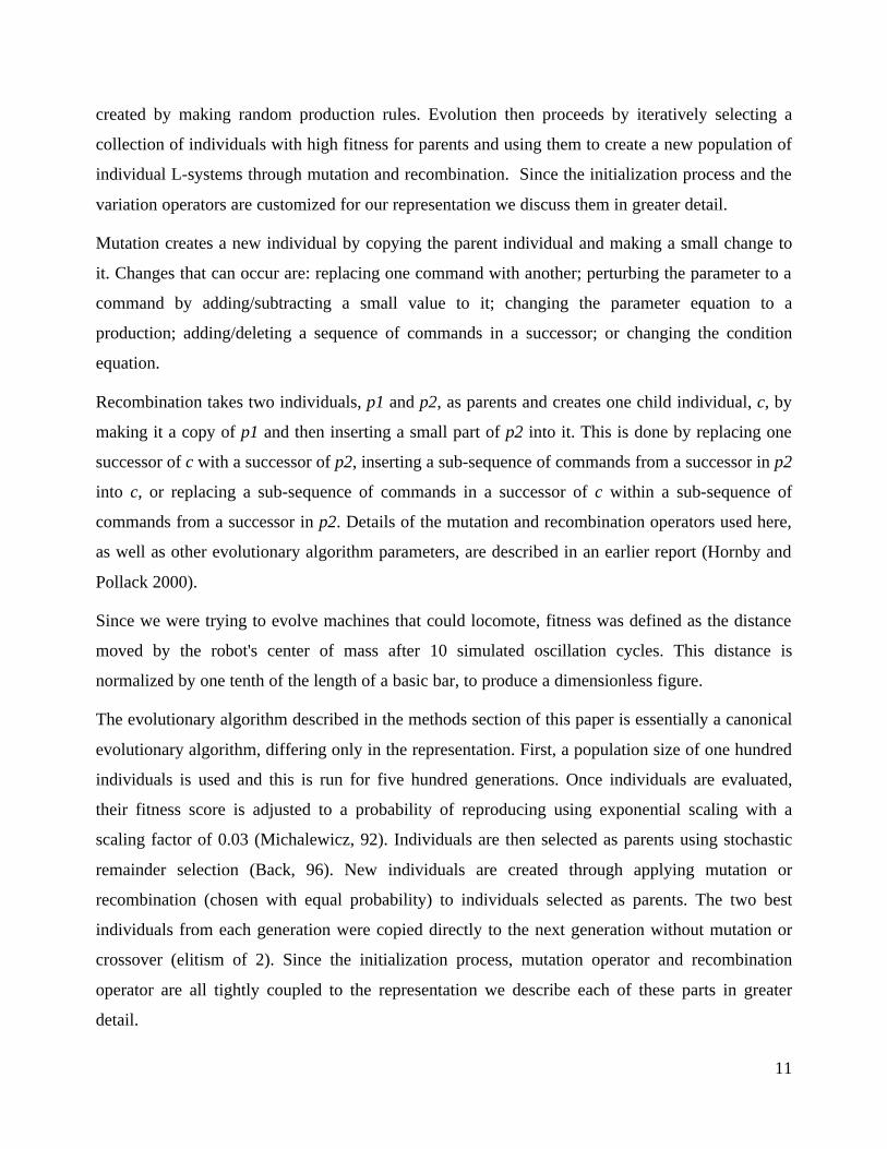
Approximately half the runs produce “interesting” viable results. Nine selected machines out of 20

runs are shown in

Figure 4. The two main forms of locomotion found used one or more oscillating appendages to

push along, or had two main body parts connected by a sequence of rods that twisted in such a way

that first one half of the robot would rotate forward, then the other. The two fastest robots evolved

with the non-generative representation, shown in

Figure 4, are #3 (fitness 1188 with 49 rods and moves by twisting) and #7 (fitness 1000 with 31

rods which moves by pushing). Half the robots had only a handful of rods, such as robot #6. Robot

#4 is an example of one that uses its appendages to roll over.

Robots evolved with the generative representation not only had higher average fitness, but tended

to move in a more continuous manner. Here the two fastest were #1 (a sequence of interlocking X's

that rolls along with fitness 2754 and 268 rods) and #5 (whose segments are shaped like a coil and

it moves by rolling sideways with fitness of 3604 and 325 rods). Not all were regular as

demonstrated by robot #2, an asymmetric robot that moves by sliding along similar to many of the

robots generated with a non-generative representation (fitness 766 and .63 rods) Robot #11 is a

four-legged walker with fitness 2170 and 109 rods. An example of the movement cycle of a robot

produced with the generative representation is shown in

, sequence a-d. This robot has fitness 686 and 80 rods and moves by passing a loop from back to

front.

5 In a true dynamics simulator actual torques on joints would be calculated and then a constraint on the allowable

torque could be used instead.

16

In general, robots evolved using the generative representation increased their speed by repeating

rolling segments to smoothen out their gaits, and increasing the size of these segments/appendages

to increase the distance moved in each oscillation.

Finally, we construct some of the evolved Genobots6. We picked three robots that were small (in

number of parts and motors) and easy to build. The “M” robot in Figure 6 shows two parts of the

locomotion cycle of the two-dimensional robot. With its two outer arms evolved to be 25% out of

phase, it moves by bringing them together to lift its middle arm and then to shift its center of mass

to the right. One modification to the constructed robot is the addition of sandpaper on the feet of the

two outer arms to compensate for the friction modeled by our simulator and that of the actual

surface used.

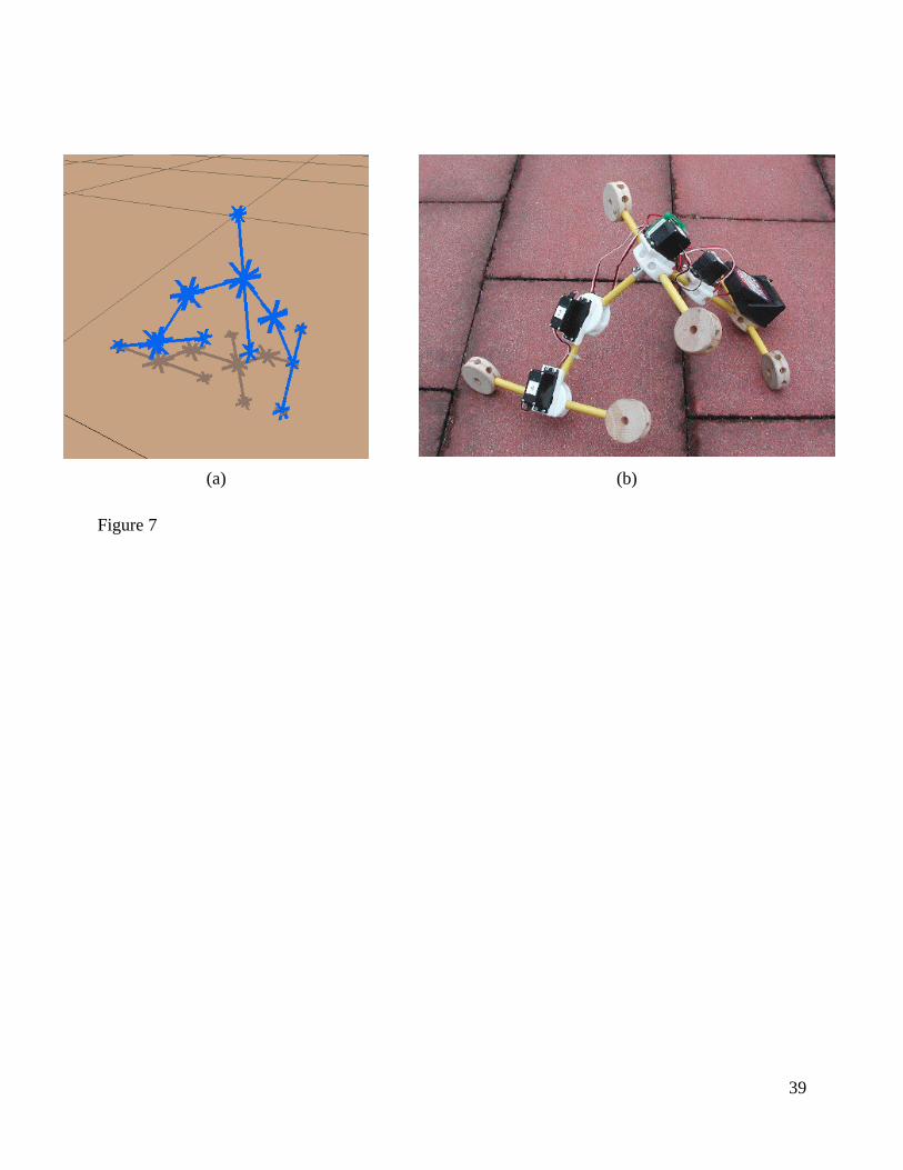
The “Kayak” robot (so called because of its form of locomotion, see video) in Figure 7 moves by

curling up in alternating directions. At the extreme stages of these oscillations, the robot contacts

the ground at only three points, freeing its fourth point to move forward. Repeated oscillations

gradually push the machine forward while its rear support is dragged across the ground.

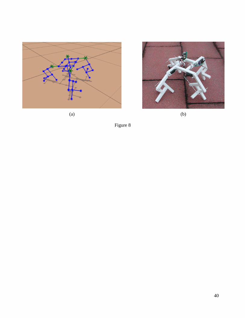
The “Quatrobot” robot in Figure 8 has one actuated joint on each of its four legs and walks by

raising and lowering its legs. Each leg 12.5% out of phase with the ones next to it and the robot

moves in the direction of the lead leg. Instead of constructing this robot out of the components in

Figure 2, it was manufactured using rapid prototyping equipment in a manner similar to our

original robots (Lipson and Pollack, 2000).

Scaling

The results shown so far demonstrate that the generative system is capable of producing non-trivial

robot designs that transfer well into reality. We now address the question of scaling – the progress

of performance of the design process over evolutionary time. This aspect determines whether

evolutionary robotics might ultimately be used as a practical engineering tool.

6 The “M” and “Kayak” robots were evolved in runs that did not use the structural constraint limiting the

maximum number of rods without a structural loop.

17

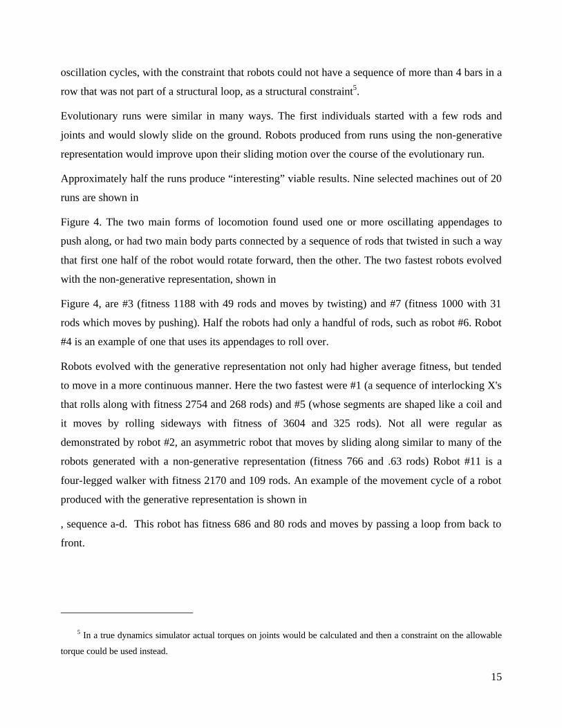
Figure 9 examines the progress of average population fitness over the generations, averaged over

10 evolutionary runs. Each run used a population of 100 individuals and was evolved for 500

generations. The lower curve corresponds to the non-generative representation, while the upper

curve shows progress for generative representation over the same substrate. It is evident that the

generative representation makes faster progress at the initial stage: Fitness increase per generation

is more than 6 times faster in the first 100 generations, as shown by the linear dashed lines. In that

short period, the generative system consistently outperforms the non-generative representation,

which does not reach an equivalent level within the entire experiment7. After around 200

generations, progress rate with the generative representation is slowed down, yet still is

approximately twice the rate of the non-generative representation.

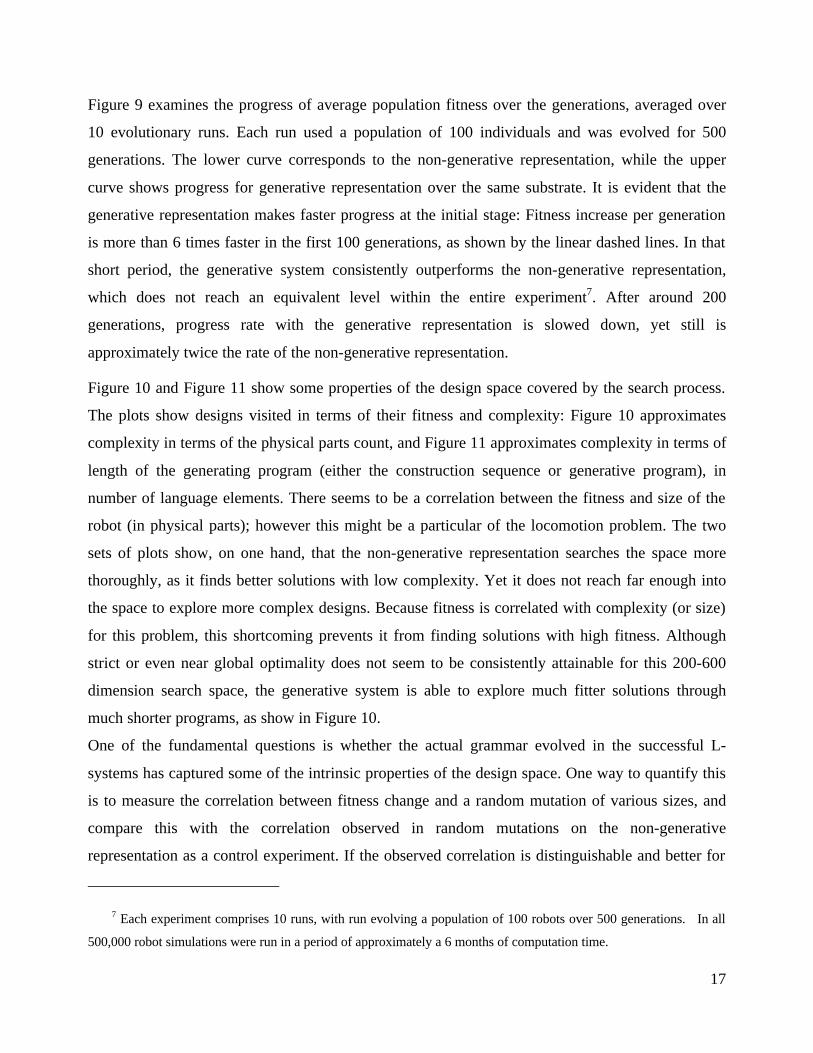
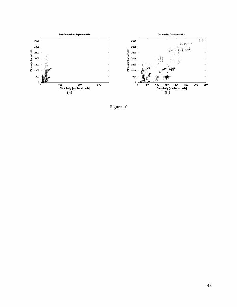
Figure 10 and Figure 11 show some properties of the design space covered by the search process.

The plots show designs visited in terms of their fitness and complexity: Figure 10 approximates

complexity in terms of the physical parts count, and Figure 11 approximates complexity in terms of

length of the generating program (either the construction sequence or generative program), in

number of language elements. There seems to be a correlation between the fitness and size of the

robot (in physical parts); however this might be a particular of the locomotion problem. The two

sets of plots show, on one hand, that the non-generative representation searches the space more

thoroughly, as it finds better solutions with low complexity. Yet it does not reach far enough into

the space to explore more complex designs. Because fitness is correlated with complexity (or size)

for this problem, this shortcoming prevents it from finding solutions with high fitness. Although

strict or even near global optimality does not seem to be consistently attainable for this 200-600

dimension search space, the generative system is able to explore much fitter solutions through

much shorter programs, as show in Figure 10.

One of the fundamental questions is whether the actual grammar evolved in the successful L-

systems has captured some of the intrinsic properties of the design space. One way to quantify this

is to measure the correlation between fitness change and a random mutation of various sizes, and

compare this with the correlation observed in random mutations on the non-generative

representation as a control experiment. If the observed correlation is distinguishable and better for

7 Each experiment comprises 10 runs, with run evolving a population of 100 robots over 500 generations. In all

500,000 robot simulations were run in a period of approximately a 6 months of computation time.

18

the generative system than it is for the blind system, then the generative system must have captured

some useful properties.

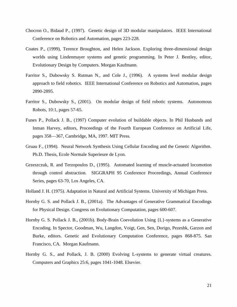
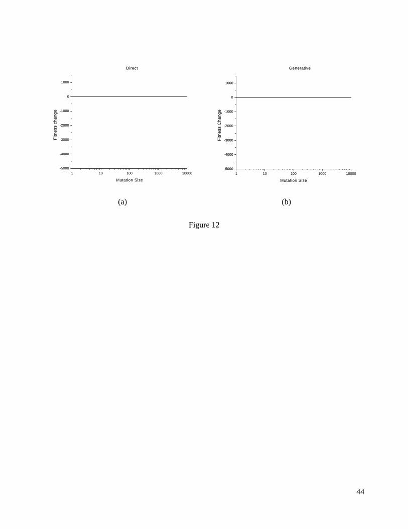
The graph in Figure 12 is a comparison of the fitness-mutation correlation between a generative

representation and a random control experiment on the same substrate and on the same set of

randomly selected individuals. For this analysis, 80,000 individuals were selected uniformly from

16 runs and over 100 generations using a generative representation. Each point represents a

particular fitness change (positive or negative) associated with a particular mutation size. The

points on the left plot (Figure 12a) were carried out on the non-generative representation generated

by the generative representation and serve as the control set. For these points, 1 to 6 mutations were

applied so as to approximate mutations of similar phenotypic-size as those on the generative

representation. Each mutation could modify or swap a sequence of characters. The points on the

right (Figure 12b) were also carried out randomly but on the generative representations of the same

randomly selected individuals. Only a single mutation was applied to the generative representation,

and consisted of modifying or swapping a single keyword or parameter. Mutation size was

measured in both cases as the number of modified commands in the final construction sequences.

The two distributions in Figure 12 have distinct features. The data points separate into two

distinguishable clusters, with some overlap. Mutations generated on the generative representations

clearly correlate with both positive fitness and negative fitness changes, whereas most mutations on

the non-generative representation result in fitness decrease. Statistics of both systems, averaged

over 8 runs each, are summarized in Table III below. A one-way ANOVA test revealed that the two

means are different with at least 95% confidence. Cross-correlation showed that in 40% of the

instances where a non-generative mutation was successful, a generative mutation was also

successful, whereas in only 20% of the instances where a generative mutation was successful, was

a non-generative mutation successful too. In both cases smaller mutations are significantly more

successful than larger mutations. However large mutations (>100) were an order of magnitude

more often successful in the generative case than in the non-generative case. All these measures

indicate that the generative representation is more efficient in exploiting useful search paths in the

design space.

19

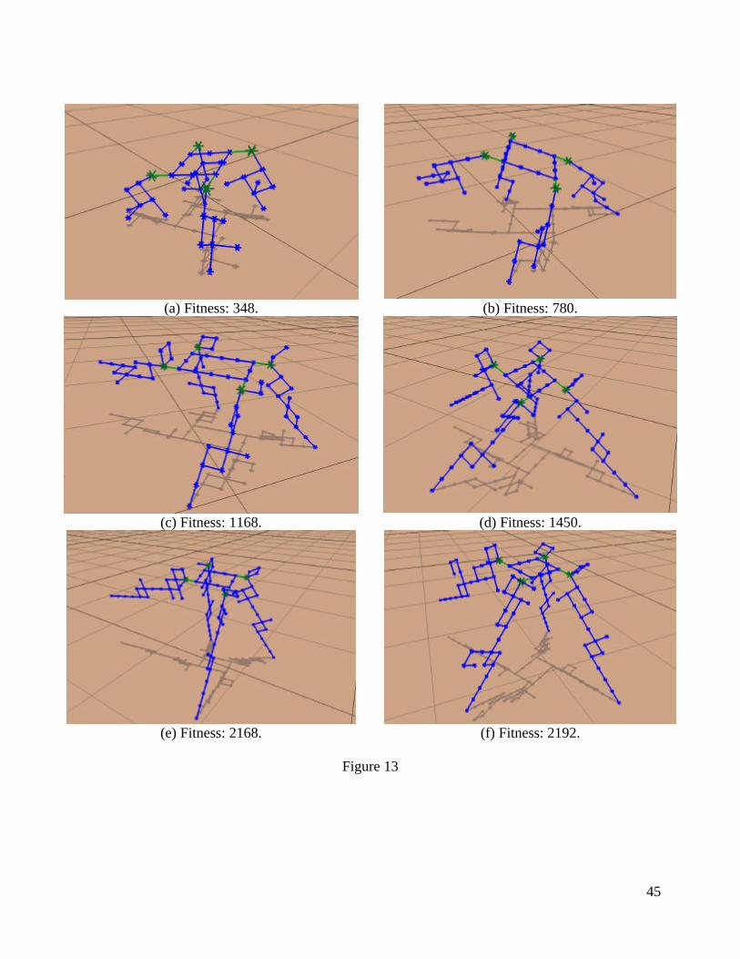
An example of how the generative representation is being used to make coordinated changes can be

seen by individuals taken from different generations of one of the evolutionary runs. The sequence

of images in Figure 13, which are the best individual in the population taken from different

generations, show two changes occurring. First, the rectangle that forms the body of the robot goes

from being two-by-two, to three-by-three, to two-by-three. This change is possible with a single

change of the generative representation but requires multiple coordinated changes on the non-

generative representation. The second change is the evolution of the robot’s legs. Even though the

legs are changing from image to image, all four legs are the same in each of the six images. As

with the body, changing all four legs simultaneously can be done easily with the generative

representation by changing the one module that is used for constructing them, but would require

simultaneously making the same change to all four occurrences of the leg assembly procedure in a

non-generative representation.

Conclusions

The purpose of the work reported in this paper is twofold. First, to demonstrate the ability of an

evolutionary process to design both the morphology and control of a physically viable three-

dimensional robot that, while it has the same basic locomotion functionality as previously evolved

machines, demonstrates a much better form of design. In this work the evolved designs are an order

of magnitude more complex, in terms of the number of given basic building blocks, than previous

work. Both the evolved designs, as well as the physically realized machines, show a significantly

higher degree of modularity, regularity and hierarchy than previous machines whose morphology

and control were generated fully automatically.

The second goal of this work is to investigate the scaling properties of generative systems when

applied to a robotic design problem. We have shown that the use of a generative representation has

significantly accelerated the rate of progress at early stages of the design search, reaching levels

that are not reached through direct mutation on the same design space and through the same

number of evaluations. Most importantly, we have shown that at least for this design space, a

generative representation is significantly more efficient in exploiting useful search paths in the

design space than a non-generative representation.

20

While the physically realized results shown here do not compare to design capabilities of teams of

human engineers, we point out that the field is still very young. Naturally, more complex machines

that can accomplish more complex tasks can be attained merely by starting with more advanced

building blocks and more sophisticated genetic operators; but the eventual inventiveness of a

design system is not measured by its final outcome, but rather by the distance of its outcome from

its starting point. We believe that careful inclusions of fundamental design principles such as

modularity, regularity, and hierarchy into self-organizing stochastic design processes like evolution

can ultimately lead to powerful design automation tools for robots which can prosper in the real

world.

Acknowledgements

This work was partially sponsored by the Defense Advanced Research Projects Administration

(DARPA grant DASG60-99-1-0004). Thanks to John Rieffel for construction help with the

Quatrobot.

References

Bäck T., Hoffmeister F, Schwefel H-P. (1991) A survey of evolution strategies. In Richard K.

Belew; Lashon B. Booker, editor, Proc. of the Fourth Int. Conf. on Genetic Algorithms, pages

2—9. Morgan Kaufmann.

Back, T., (1996). Evolutionary Algorithms in Theory and Practice. Oxford University Press, New

York.

Bentley P. J. (1996) Generic Evolutionary Design of Solid Objects Using a Genetic Algorithm.

PhD thesis, University of Huddersfield

Bentley P. J., (ed.). (1999) Evolutionary Design by Computers. Morgan Kaufman

Bentley P., Kumar S. (1999). Three ways to grow designs: A comparison of embryogenies of an

evolutionary design problem. In Banzhaf, Daida, Eiben, Garzon, Honavar, Jakiel, and Smith,

editors, Proc. Genetic and Evolutionary Computation Conference, pages 35—43.

Chen I., Burdick J., (1995). Determining task optimal robot assembly configurations. IEEE

International Conference on Robotics and Automation, pages 132-137.

21

Chocron O., Bidaud P., (1997). Genetic design of 3D modular manipulators. IEEE International

Conference on Robotics and Automation, pages 223-228.

Coates P., (1999), Terence Broughton, and Helen Jackson. Exploring three-dimensional design

worlds using Lindenmayer systems and genetic programming. In Peter J. Bentley, editor,

Evolutionary Design by Computers. Morgan Kaufmann.

Farritor S., Dubowsky S. Rutman N., and Cole J., (1996). A systems level modular design

approach to field robotics. IEEE International Conference on Robotics and Automation, pages

2890-2895.

Farritor S., Dubowsky S., (2001). On modular design of field robotic systems. Autonomous

Robots, 10:1, pages 57-65.

Funes P., Pollack J. B., (1997) Computer evolution of buildable objects. In Phil Husbands and

Inman Harvey, editors, Proceedings of the Fourth European Conference on Artificial Life,

pages 358—367, Cambridge, MA, 1997. MIT Press.

Gruau F., (1994). Neural Network Synthesis Using Cellular Encoding and the Genetic Algorithm.

Ph.D. Thesis, Ecole Normale Superieure de Lyon.

Grzeszczuk, R. and Terzopoulos D., (1995). Automated learning of muscle-actuated locomotion

through control abstraction. SIGGRAPH 95 Conference Proceedings, Annual Conference

Series, pages 63-70, Los Angeles, CA.

Holland J. H. (1975). Adaptation in Natural and Artificial Systems. University of Michigan Press.

Hornby G. S. and Pollack J. B., (2001a). The Advantages of Generative Grammatical Encodings

for Physical Design. Congress on Evolutionary Computation, pages 600-607.

Hornby G. S. Pollack J. B., (2001b). Body-Brain Coevolution Using {L}-systems as a Generative

Encoding. In Spector, Goodman, Wu, Langdon, Voigt, Gen, Sen, Dorigo, Pezeshk, Garzon and

Burke, editors. Genetic and Evolutionary Computation Conference, pages 868-875. San

Francisco, CA. Morgan Kaufmann.

Hornby G. S., and Pollack, J. B. (2000) Evolving L-systems to generate virtual creatures.

Computers and Graphics 25:6, pages 1041-1048. Elsevier.

22

Hornby G. S., Fujita M., Takamura S., and Yamamoto T., (1999). Autonomous evolution of gaits

with the Sony quadruped robot. In Banzhaf W., Daida J., Eiben A. E., Garzon M., Honavar V.,

Jakiela M., and Smith R. E., editors. Proceedings of the Genetic and Evolutionary Computation

Conference. Morgan Kaufmann.

Hornby G. S., Takamure S., Hanagata O. and Fujita M., (2000). Evolution of Controllers from a

High-Level Simulator to a High DOF Robot. In Miller J., editor. Evolvable Systems: from

biology to hardware; Proceedings of the Third Intl. Conf., Lecture Notes in Computer Science;

Vol. 1801, pages 80-89. Springer.

Hornby, G. S., Pollack, J. B. “Creating High-level Components with a Generative Representation

for Body-Brain Evolution” Artificial Life (in press)

Husbands P., Germy G., McIlhagga M., Ives R.. (1996) Two applications of genetic algorithms to

component design. In T. Fogarty, editor, Evolutionary Computing. LNCS 1143, pages 50—61.

Springer-Verlag,

Jacob C. (1994) Genetic L-system Programming. In Y. Davidor and P. Schwefel, editors, Parallel

Problem Solving from Nature, Lecture Notes in Computer Science, volume 866, pages 334—

343. Springer-Verlag

Jakobi N., (1998). Minimal Simulations for Evolutionary Robotics, Ph.D. Thesis, School of

Cognitive and Computing Sciences, University of Sussex

Kane C., Schoenauer M, (1995). Genetic operators for two-dimentional shape optimization. In J.-

M. Alliot, E. Lutton, E. Ronald, M. Schoenauer, and D. Snyers, editors, Artificiale Evolution -

EA95. Springer-Verlag

Kim J.-O., Khosla P. K.(1993). Design of space shuttle tile servicing robot: an application of task

based kinematic design. IEEE International Conference on Robotics and Automation, pages

867-874.

Komosinski M., Rotaru-Varga A (2000). From directed to open-ended evolution in a complex

simulation model. In Bedau, McCaskill, Packard, and Rasmussen, editors, Artificial Life 7,

pages 293—299. Morgan Kaufmann.

Koza J. R. (1992). Genetic Programming: on the programming of computers by means of natural

selection. MIT Press. Cambridge, MA.

23

Leger P. C., (1999). Automated synthesis and optimization of robot configurations: an

evolutionary approach. Ph.D. Thesis, The Robotics Institute, Carnegie Mellon University.

Pittsburgh, PA.

Lindenmayer A (1968). Mathematical models for cellular interaction in development, parts I and II.

Journal of Theoretical Biology, 18:280—299 and 300—315

Lindenmayer A. (1974). Adding continuous components to L-Systems. In G. Rozenberg and A.

Salomaa, editors, L Systems, Lecture Notes in Computer Science 15, pages 53—68. Springer-

Verlag, 1974.

Lipson H., Pollack J.B. (2000). Automatic design and manufacture of robotic lifeforms. Nature,

406:974—978

M. Mataric & D. Cliff (1996)``Challenges in Evolving Controllers for Physical Robots'' Robotics

and Autonomous Systems 19(1):67--83, 1996.

Maynard-Smith, J, and E. Szathmary. (1995) The major transitions in evolution. Oxford: Oxford

Press.

Michalewicz, Z., (1992). Genetic Algorithms + Data Structures = Evolution Programs. Springer-

Verlag, New York

Ngo J. T., and Marks J., (1993). Spacetime Constraints Revisited. In SIGGRAPH 93 Conference

Proceedings, Annual Conference Series, pages 343-350.

Nolfi, S. & Floreano, D. Evolutionary Robotics. The Biology, Intelligence, and Technology of Self-

organizing Machines. Cambridge, MA: MIT Press, 2000

Ochoa G. (1998). On genetic algorithms and lindenmayer systems. In A. Eiben, T. Baeck, M.

Schoenauer, and H. P. Schwefel, editors, Parallel Problem Solving from Nature V, pages 335—

344. Springer-Verlag.

Paredis C., (1996). An agent-based approach to the design of rapidly deployable fault tolerant

manipulators. Ph.D. Thesis, Dept. of Electrical and Computer Engineering, CMU. Pittsburgh,

PA.

Pollack J. B., Lipson H., Ficici S., Funes P., Hornby G., Watson R., (2000). Evolutionary

techniques in physical robotics. In Miller J., editor, Evolvable Systems: from biology to

24

hardware; Proc. Of the Third Intl. Conf., pages 175-186. Lecture Notes In Computer Science;

Vol. 1801. Springer.

Prusinkiewicz P., Lindenmayer A (1990). The Algorithmic Beauty of Plants. Springer-Verlag

Roston G. P., (1994). A genetic methodology for configuration design. Ph. D. Thesis, Dept. of

Mechanical Engineering, Carnegie Mellon University.

Schoenauer M (1996). Shape representations and evolution schemes. In L. J. Fogel, P. J. Angeline,

and T. Back, editors, Evolutionary Programming 5. MIT Press, 1996.

Simon, H., (1969). The sciences of the artificial. MIT Press. Cambridge, MA.

Sims K. (1994). Evolving Virtual Creatures. In SIGGRAPH 94 Conference Proceedings, Annual

Conference Series, pages 15—22

Watson, R.A. and Pollack, J.B. (To appear). A Computational Model of Symbiotic Composition in

Evolutionary Transitions. Biosystems,

25

Appendix

Generative representation for robot “M”

Generative Representation Construction Sequence This generative representation is started with P0(3.0,3.0) and run for ten

iterations. (T) indicates that the condition always succeeds. P0: (n0>3.0) :- clockwise(1.0) cntr-clockwise(n1) [clockwise(1.0) clockwise(1.0)

back(5.0) ] (n0>3.0) :- clockwise(1.0) cntr-clockwise(n1) [clockwise(1.0) clockwise(1.0)

back(5.0) ] (T) :- [cntr-clockwise(1.0) P7(n0+1.0,n1-n0) ] P1: (n0>3.0) :- [clockwise(1.0) ] (n0>3.0) :- [clockwise(1.0) ] (T) :- P0(n1,n0-1.0) clockwise(1.0) {forward(1.0) }(2.0) P3: (n1>5.0) :- clockwise(1.0) decrease-offset(1.0) P8(5.0,n0/5.0) decrease-

offset(1.0) (n1>1.0) :- clockwise(1.0) cntr-clockwise(n1) [clockwise(1.0) clockwise(1.0)

back(5.0) ] (T) :- clockwise(1.0) cntr-clockwise(n1) clockwise(1.0) clockwise(1.0)

back(5.0) P5: (n1>3.0) :- {joint(5.0) }(3.0) P6(n1-2.0,n0/n1) back(1.0) (n1>3.0) :- {joint(5.0) }(3.0) back(1.0) P6(n1-2.0,n0/n1) (T) :- P12(n1/3.0,5.0) back(1.0) P6: (n1>3.0) :- [clockwise(1.0) clockwise(n1) ] (n1>3.0) :- [clockwise(1.0) clockwise(n1) ] (T) :- forward(2.0) decrease-offset(1.0) cntr-clockwise(1.0)

P13(n1+1.0,n1/n0) forward(1.0) P7: (n1>1.0) :- {cntr-clockwise(1.0) decrease-offset(1.0) }(1.0) (n1>1.0) :- {cntr-clockwise(1.0) decrease-offset(1.0) }(1.0) (T) :- clockwise(1.0) [cntr-clockwise(1.0) ] P9(n1+1.0,n1+1.0) P3(n1-

4.0,n1+1.0) P9: (n1>1.0) :- [P11(1.0,n0+2.0) P10(n0+5.0,n0) cntr-clockwise(1.0) ] (n1>1.0) :- [P11(1.0,n0+2.0) P10(n0+5.0,n0) cntr-clockwise(1.0) ] (T) :- clockwise(n0) increase-offset1.0) cntr-clockwise(5.0) P3(3.0,3.0)

P6(n1-1.0,1.0) P13: (n1>4.0) :- [P14(n0-n1,n1+2.0) cntr-clockwise(1.0) ] (n1>4.0) :- [P14(n0-n1,n1+2.0) cntr-clockwise(1.0) ]

(T) :- [P5(n0,n1+4.0) ] [P1(n1+n0,5.0) cntr-clockwise(3.0) ]

[ cntr-clockwise(1) clockwise(1) [ cntr-clockwise(1) ] clockwise(1) offset-increase(1) cntr-clockwise(5) clockwise(1) cntr-clockwise(3) [ clockwise(1) clockwise(1) back(5) ] forward(2) offset-decrease(1) cntr-clockwise(1) [ joint(5) joint(5) joint(5) forward(2) offset-decrease(1) cntr-clockwise(1) [ joint(5) joint(5) joint(5) forward(2) offset-decrease(1) cntr-clockwise(1) forward(1) back(1) ] [ clockwise(1) cntr-clockwise(0) [ clockwise(1) clockwise(1) back(5) ] clockwise(1) forward(1) forward(1) cntr-clockwise(3) ] forward(1) back(1) ] [ clockwise(1) cntr-clockwise(2) [ clockwise(1) clockwise(1) back(5) ] clockwise(1) forward(1) forward(1) cntr-clockwise(3) ] forward(1) clockwise(1) cntr-clockwise(1) clockwise(1) clockwise(1) back(5) ] See Table I for meaning of commands.

26

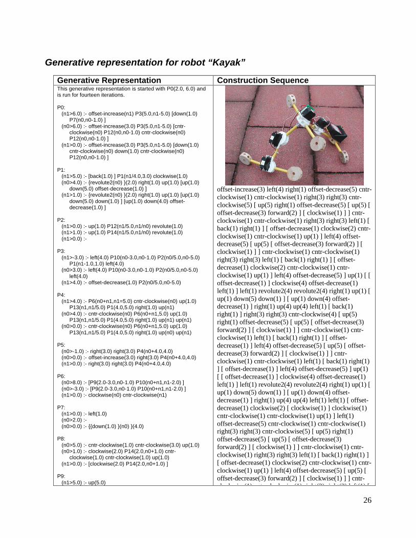
Generative representation for robot “Kayak”

Generative Representation Construction Sequence This generative representation is started with P0(2.0, 6.0) and is run for fourteen iterations. P0: (n1>6.0) :- offset-increase(n1) P3(5.0,n1-5.0) [down(1.0)

P7(n0,n0-1.0) ] (n0>6.0) :- offset-increase(3.0) P3(5.0,n1-5.0) [cntr-

clockwise(n0) P12(n0,n0-1.0) cntr-clockwise(n0) P12(n0,n0-1.0) ]

(n1>0.0) :- offset-increase(3.0) P3(5.0,n1-5.0) [down(1.0) cntr-clockwise(n0) down(1.0) cntr-clockwise(n0) P12(n0,n0-1.0) ]

P1: (n1>5.0) :- [back(1.0) ] P1(n1/4.0,3.0) clockwise(1.0) (n0>4.0) :- {revolute2(n0) }(2.0) right(1.0) up(1.0) [up(1.0)

down(5.0) offset-decrease(1.0) ] (n1>1.0) :- {revolute2(n0) }(2.0) right(1.0) up(1.0) [up(1.0)

down(5.0) down(1.0) ] [up(1.0) down(4.0) offset-decrease(1.0) ]

P2: (n1>0.0) :- up(1.0) P12(n1/5.0,n1/n0) revolute(1.0) (n1>1.0) :- up(1.0) P14(n1/5.0,n1/n0) revolute(1.0) (n1>0.0) :- P3: (n1>-3.0) :- left(4.0) P10(n0-3.0,n0-1.0) P2(n0/5.0,n0-5.0)

P1(n1-1.0,1.0) left(4.0) (n0>3.0) :- left(4.0) P10(n0-3.0,n0-1.0) P2(n0/5.0,n0-5.0)

left(4.0) (n1>4.0) :- offset-decrease(1.0) P2(n0/5.0,n0-5.0) P4: (n1>4.0) :- P6(n0+n1,n1=5.0) cntr-clockwise(n0) up(1.0)

P13(n1,n1/5.0) P1(4.0,5.0) right(1.0) up(n1) (n0>4.0) :- cntr-clockwise(n0) P6(n0+n1,5.0) up(1.0)

P13(n1,n1/5.0) P1(4.0,5.0) right(1.0) up(n1) up(n1) (n0>0.0) :- cntr-clockwise(n0) P6(n0+n1,5.0) up(1.0)

P13(n1,n1/5.0) P1(4.0,5.0) right(1.0) up(n0) up(n1) P5: (n0>-1.0) :- right(3.0) right(3.0) P4(n0+4.0,4.0) (n0>0.0) :- offset-increase(3.0) right(3.0) P4(n0+4.0,4.0) (n1>0.0) :- right(3.0) right(3.0) P4(n0+4.0,4.0) P6: (n0>8.0) :- [P9(2.0-3.0,n0-1.0) P10(n0+n1,n1-2.0) ] (n0>-3.0) :- [P9(2.0-3.0,n0-1.0) P10(n0+n1,n1-2.0) ] (n1>0.0) :- clockwise(n0) cntr-clockwise(n1) P7: (n1>0.0) :- left(1.0) (n0>2.0) :- (n0>0.0) :- {{down(1.0) }(n0) }(4.0) P8: (n0>5.0) :- cntr-clockwise(1.0) cntr-clockwise(3.0) up(1.0) (n0>1.0) :- clockwise(2.0) P14(2.0,n0+1.0) cntr-

clockwise(1.0) cntr-clockwise(1.0) up(1.0) (n1>0.0) :- [clockwise(2.0) P14(2.0,n0+1.0) ] P9: (n1>5.0) :- up(5.0)

offset-increase(3) left(4) right(1) offset-decrease(5) cntr-clockwise(1) cntr-clockwise(1) right(3) right(3) cntr-clockwise(5) [ up(5) right(1) offset-decrease(5) [ up(5) [ offset-decrease(3) forward(2) ] [ clockwise(1) ] ] cntr-clockwise(1) cntr-clockwise(1) right(3) right(3) left(1) [ back(1) right(1) ] [ offset-decrease(1) clockwise(2) cntr-clockwise(1) cntr-clockwise(1) up(1) ] left(4) offset-decrease(5) [ up(5) [ offset-decrease(3) forward(2) ] [ clockwise(1) ] ] cntr-clockwise(1) cntr-clockwise(1) right(3) right(3) left(1) [ back(1) right(1) ] [ offset-decrease(1) clockwise(2) cntr-clockwise(1) cntr-clockwise(1) up(1) ] left(4) offset-decrease(5) ] up(1) [ [ offset-decrease(1) ] clockwise(4) offset-decrease(1) left(1) ] left(1) revolute2(4) revolute2(4) right(1) up(1) [ up(1) down(5) down(1) ] [ up(1) down(4) offset-decrease(1) ] right(1) up(4) up(4) left(1) [ back(1) right(1) ] right(3) right(3) cntr-clockwise(4) [ up(5) right(1) offset-decrease(5) [ up(5) [ offset-decrease(3) forward(2) ] [ clockwise(1) ] ] cntr-clockwise(1) cntr-clockwise(1) left(1) [ back(1) right(1) ] [ offset-decrease(1) ] left(4) offset-decrease(5) [ up(5) [ offset-decrease(3) forward(2) ] [ clockwise(1) ] ] cntr-clockwise(1) cntr-clockwise(1) left(1) [ back(1) right(1) ] [ offset-decrease(1) ] left(4) offset-decrease(5) ] up(1) [ [ offset-decrease(1) ] clockwise(4) offset-decrease(1) left(1) ] left(1) revolute2(4) revolute2(4) right(1) up(1) [ up(1) down(5) down(1) ] [ up(1) down(4) offset-decrease(1) ] right(1) up(4) up(4) left(1) left(1) [ offset-decrease(1) clockwise(2) [ clockwise(1) ] clockwise(1) cntr-clockwise(1) cntr-clockwise(1) up(1) ] left(1) offset-decrease(5) cntr-clockwise(1) cntr-clockwise(1) right(3) right(3) cntr-clockwise(5) [ up(5) right(1) offset-decrease(5) [ up(5) [ offset-decrease(3) forward(2) ] [ clockwise(1) ] ] cntr-clockwise(1) cntr-clockwise(1) right(3) right(3) left(1) [ back(1) right(1) ] [ offset-decrease(1) clockwise(2) cntr-clockwise(1) cntr-clockwise(1) up(1) ] left(4) offset-decrease(5) [ up(5) [ offset-decrease(3) forward(2) ] [ clockwise(1) ] ] cntr-clockwise(1) cntr-clockwise(1) right(3) right(3) left(1) [

27

(n1>1.0) :- P5(n0-1.0,n0/5.0) P7(n1/n0,5.0/4.0) P7(n1/n0,n1/1.0)

(n0>0.0) :- P5(n0-1.0,n0/5.0) P10: (n1>4.0) :- [offset-decrease(3.0) forward(2.0) ]

[clockwise(1.0) ] (n1>3.0) :- right(1.0) {offset-decrease(5.0) P11(3.0,n1+n0)

P6(n0-5.0,n0-4.0) }(2.0) (n1>0.0) :- right(1.0) {offset-decrease(5.0) P6(n0-5.0,n0-4.0)

P11(4.0,n1+n0) }(2.0) offset-decrease(5.0) P11: (n0>1.0) :- cntr-clockwise(1.0) P11(n0/4.0,n0+n1) (n0>0.0) :- cntr-clockwise(1.0) P9(n1/4.0,n0-1.0)

P12(n1/5.0,5.0) (n0>0.0) :- cntr-clockwise(1.0) P12(n1/5.0,5.0) P12: (n1>1.0) :- left(1.0) [back(1.0) right(1.0) ] P9(n1-4.0,3.0)

[offset-decrease(1.0) P8(n1,n1+n0) ] left(n0) (n1>-1.0) :- left(1.0) [back(1.0) down(n0) ] P9(n1-4.0,3.0)

left(n1) (n1>0.0) :- [back(1.0) down(n0) ] [P8(n0,n0-n1) ] P13: (n0>4.0) :- left(1.0) P12(4.0,1.0-2.0) (n0>3.0) :- [[offset-decrease(1.0) ] clockwise(4.0) offset-

decrease(1.0) left(1.0) ] left(1.0) P12(4.0,1.0-2.0) (n1>0.0) :- left(1.0) clockwise(4.0) P14: (n0>5.0) :- (n0>5.0) :- clockwise(1.0) P5(n1+n0,n1/5.0) (n0>0.0) :- [clockwise(1.0) ] clockwise(1.0)

clockwise(1) cntr-clockwise(1) right(3) right(3) left(1) [ back(1) right(1) ] [ offset-decrease(1) clockwise(2) cntr-clockwise(1) cntr-clockwise(1) up(1) ] left(4) offset-decrease(5) ] up(1) [ [ offset-decrease(1) ] clockwise(4) offset-decrease(1) left(1) ] left(1) revolute2(4) revolute2(4) right(1) up(1) [ up(1) down(5) down(1) ] [ up(1) down(4) offset-decrease(1) ] right(1) up(4) up(4) left(1) [ back(1) right(1) ] right(3) right(3) cntr-clockwise(4) [ up(5) right(1) offset-decrease(5) [ up(5) [ offset-decrease(3) forward(2) ] [ clockwise(1) ] ] cntr-clockwise(1) cntr-clockwise(1) left(1) [ back(1) right(1) ] [ offset-decrease(1) ] left(4) offset-decrease(5) [ up(5) [ offset-decrease(3) forward(2) ] [ clockwise(1) ] ] cntr-clockwise(1) cntr-clockwise(1) left(1) [ back(1) right(1) ] [ offset-decrease(1) ] left(4) offset-decrease(5) ] up(1) [ [ offset-decrease(1) ] clockwise(4) offset-decrease(1) left(1) ] left(1) revolute2(4) revolute2(4) right(1) up(1) [ up(1) down(5) down(1) ] [ up(1) down(4) offset-decrease(1) ] right(1) up(4) up(4) left(1) left(1) [ offset-decrease(1) clockwise(2) [ clockwise(1) ] clockwise(1) cntr-clockwise(1) cntr-clockwise(1) up(1) ] left(1) left(4) [ down(1) cntr-clockwise(2) down(1) cntr-clockwise(2) left(1) [ back(1) down(2) ] left(1) left(1) left(1) ] See Table II for meaning of commands.

28

Generative representation for robot “Quatrobot”

Generative Representation Construction Sequence This generative representation is started with P0(5.0,4.0) and run

thirten iterations. (T) indicates that the condition always succeeds. The assembly procedure is not included because it consists of almost 900 commands.

P0: (n1>1.0) :- [P12(n0-0.0,n1-0.0) ] [P3(4.0,n1/1.0) forward(1.0)

P0(n1/2.0,5.0) decrease-offset(n0) ] (n1>0.0) :- [decrease-offset(1.0) cntr-clockwise(1.0) left(1.0)

forward(1.0) ] increase-offset(1.0) P1: (n1>1.0) :- increase-offset(1.0) P8(n1,n0+5.0) [P7(n1-

n0,n1+n0) right(5.0) P10(n1/n0,n0-4.0) increase-offset(1.0) ] left(1.0) forward(1.0) clockwise(1.0)

(n0>0.0) :- decrease-offset(1.0) P3: (n1>2.0) :- [forward(1.0) revolute(n1) down(1.0) forward(1.0)

P6(n0+2.0,3.0) increase-offset(1.0) forward(1.0) ] forward(1.0) right(1.0) increase-offset(1.0)

(n1>0.0) :- [forward(1.0) revolute(n1) forward(1.0) down(1.0) P6(n0+2.0,3.0) increase-offset(1.0) forward(1.0) ] forward(1.0) right(1.0) increase-offset(1.0)

P4: (n1>6.0) :- [forward(n0) down(1.0) ] forward(n0) [down(1.0) ]

[left(1.0) forward(1.0) ] [P7(n1-n0,n1/5.0) cntr-clockwise(3.0) ] revolute(1.0) back(5.0) P1(2.0,n1/2.0)

(n0>0.0) :- [forward(n0) down(1.0) ] [forward(n0) down(1.0) ] [left(1.0) forward(1.0) ] [P7(n1-n0,n1/5.0) cntr-clockwise(3.0) ] revolute(1.0) back(5.0) P1(2.0,n1/2.0)

P6: (n0>2.0) :- right(1.0) down(1.0) [forward(1.0) forward(1.0) ]

[right(5.0) cntr-clockwise(2.0) ] increase-offset(n1) P4(n0-2.0,n1+3.0) back(n1) left(1.0)

(n0>0.0) :- [right(1.0) revolute2(1.0) revolute2(1.0) left(1.0) ] [cntr-clockwise(n1) left(n1) up(n0) left(4.0) ]

P7: (n1>2.0) :- clockwise(n0) clockwise(n0) (n1>0.0) :- [decrease-offset(1.0) forward(1.0) increase-

offset(1.0) ] clockwise(n0) clockwise(n0) P8: (n1>5.0) :- forward(5.0) left(1.0) cntr-clockwise(1.0)

clockwise(1.0) decrease-offset(1.0) forward(5.0) cntr-clockwise(1.0) [clockwise(3.0) revolute2(1.0) left(1.0) ]

(n1>0.0) :- back(1.0) P10: (n1>-2.0) :- forward(n1) P14(n1-5.0,n0/3.0) [increase-offset(3.0)

increase-offset(1.0) right(1.0) ] [up(1.0) ] {right(1.0) }(2.0) (n0>0.0) :- P14(n1-5.0,n0/3.0) forward(n1) [increase-offset(3.0)

increase-offset(1.0) up(1.0) ] [up(1.0) ] {right(1.0) }(2.0) P12: (n1>3.0) :- clockwise(2.0) up(5.0) up(4.0) (n1>0.0) :- clockwise(2.0) forward(5.0) up(4.0) P14: (n1>2.0) :- [P0(n0+1.0,n0/3.0) down(5.0) increase-offset(1.0)

clockwise(3.0) ] down(n0) down(4.0) back(1.0) down(1.0)

(Construction sequence has not been included do to its length)

29

down(1.0) decrease-offset(1.0) (n0>0.0) :- up(1.0) right(1.0) forward(4.0) P14(2.0,n1-2.0)

P8(3.0,n0+2.0) forward(1.0) clockwise(1.0) decrease-offset(1.0) back(1.0) forward(1.0) increase-offset(1.0)

30

List of footnotes (besides those appearing on title page)

3. However, note that because of the stochastic nature of the process, it is hard to determine definitely whether progress has actually halted, and improvements may still occur after long periods of apparent stagnation (Figures 1c and 1d).

4. This real time lingering is amplified by the fact that evaluation time or duration of a generation (in simulation or in physical reality) also increases as solutions become more complex

5. In a true dynamics simulator actual torques on joints would be calculated and then a constraint on the allowable torque could be used instead.

6. The “M” and “Kayak” robots were evolved in runs that did not use the structural constraint limiting the maximum number of rods without a structural loop.

7. Each experiment comprises 10 runs, with run evolving a population of 100 robots over 500 generations. In all 500,000 robot simulations were run in a period of approximately a 6 months of computation time.

31

Figure Captions

Figure 1. Progress of a typical evolutionary design run comprising only direct mutations. The abscissa represents evolutionary time (generations) and the ordinate measures fitness. Each point in the scatter plot represents one candidate design. In general, a logarithmic slowdown in progress can be observed, characterized by longer and longer durations between successive step-jumps in the fitness (a,b). Occasionally, however, progress is made after long periods of stagnation (c,d).

Figure 2. Basic building blocks of the system: bars of regular lengths and fixes or actuated joints.

Figure 3. Sample L-Robot, (a) a construction sequence leading to a tri-star 2D robot with three

actuated joints, (b) resulting robot, with joints at 180°, and (c) with joints at 120°

Figure 4. Evolved robots through non-generative and generative representations. (For full motion

see videos at http://www.demo.cs.brandeis.edu/pr/evo_design/evo_design.html)

Figure 5. The locomotion cycle of a 80-rod robot evolved using generative representation and

reaching a fitness of 686. The robot moves by passing a loop from back to front. Frames (a-d) show

four stages in the locomotion cycle. (For full motion see video at

http://www.demo.cs.brandeis.edu/pr/evo_design/evo_design.html)

Figure 6. Two parts of the locomotion cycle of an evolved two-dimensional robot “M”. (a, b)

Simulated, (c, d) physical. Notice regularity and symmetry.

Figure 7. An evolved 3D robot “Kayak”, (a) Simulated, (b) physical. Notice the reuse of a T-

junction.

Figure 8. An evolved 3D robot “Quatrobot”, (a) Simulated, (b) physical. Notice the reuse of the leg

assembly. For video of the robots in motion see

http://www.demo.cs.brandeis.edu/pr/evo_design/evo_design/html

32

Figure 9. Fitness over time, comparing non-generative representation with generated

representation. Data averaged over 10 runs.

Figure 10. Comparison of fitness versus number of parts: (a) non-generative representation; (b)

generative representation. One dot for the best individual of each generation for all 10 runs.

Figure 11. Comparison of fitness versus length of generating program, measured in number of

elements in encoded design: (a) non-generative representation; (b) generative representation. One

dot for the best individual of each generation for all ten runs.

Figure 12. Comparison of fitness change per mutation, in (a) non-generative representation and (b)

generative representation

Figure 13. Evolution of a four-legged walking robot.

33

(a) (b)

(c) (d)

Figure 1

34

Figure 2

35

forward(1)

push, joint(1), forward(1)

pop, clockwise(2)

joint(1), push, joint(1), forward(1), pop, clockwise(2)

joint(1), push, joint(1), forward(1), pop, clockwise(2)

Turtle Bar Actuator

(b)

(a) (c)

Figure 3

36

#3, Non-generative #4, Non-generative #6, Non-generative

#7, Non-generative #9, Non-generative #1, Generative

#2, Generative #5, Generative #11, Generative

Figure 4

37

(a) (b)

(c) (d)

Figure 5

38

(a) (b)

(c) (d)

Figure 6

39

(a) (b)

Figure 7

40

(a) (b)

Figure 8

41

0 100 200 300 400 5000

200

400

600

800

1000

1200

1400

Average Fitness of Population

Fitn

ess

[Vel

ocity

]

Generations

Generative Direct Linear fit to first 100 generations

Figure 9

42

(a) (b)

Figure 10

43

(a) (b)

Figure 11

44

1 10 100 1000 10000-5000

-4000

-3000

-2000

-1000

0

1000

Direct

Fitn

ess

chan

ge

Mutation Size

1 10 100 1000 10000-5000

-4000

-3000

-2000

-1000

0

1000

Generative

Fitn

ess

Cha

nge

Mutation Size

(a) (b)

Figure 12

45

(a) Fitness: 348. (b) Fitness: 780.

(c) Fitness: 1168. (d) Fitness: 1450.

(e) Fitness: 2168. (f) Fitness: 2192.

Figure 13

46

Table I: Design Language for 2D robot

Command Description [ ] Push/pop orientation stack { block }(n) Repeat enclosed block n times Forward(n) moves the turtle forward in the current direction,

creating a bar if none exists or traversing to the end of the existing bar

Back(n) Move up n levels of parents Joint(n) Forward, end with an actuated joint which

oscillates at speed n Clockwise(n) Rotate heading clockwise n × 60° CounterClockwise(n) Rotate heading counterclockwise n × 60° IncreaseOffset(n) Increase current joint phase offset by n × 25% DecreaseOffset(n) Decrease current joint phase offset by n × 25%

47

Table II: Design Language for 3D robot

Command Description [ ] Push/pop orientation stack { block }(n) Repeat enclosed block n times Forward(n) moves the turtle forward in the current direction,

creating a bar if none exists or traversing to the end of the existing bar

Back(n) Move up n levels of parents Revolute1(n) Forward, end with a joint with range 0° to 90° about the

current Z-axis that oscillates with speed n. Revolute2(n) Forward, end with a joint with range –45° to +45° about

the current Z-axis that oscillates with speed n. Twist90(n) Forward, end with a joint with range 0° to 90° about the

current X-axis that oscillates with speed n. Twist180(n) Forward, end with a joint with range -90° to +180° about

the current X-axis that oscillates with speed n. Up(n) Rotate heading n times 90° about the turtle's Z axis Down(n) Rotate heading n times -90° about the turtle's Z axis Left(n) Rotate heading n times 90° about the turtle's Y axis Right(n) Rotate heading n times -90° about the turtle's Y axis Clockwise(n) Rotate heading clockwise n × 90° about the turtle's Z

axis CounterClockwise(n) Rotate heading counterclockwise n × -90° about the

turtle's Z axis IncreaseOffset(n) Increase current joint phase offset by n × 25% DecreaseOffset(n) Decrease current joint phase offset by n × 25%

48

Table III: Evolvability comparison

Statistics for the experiments Non-generative (Control)

Generative

Average fitness change –502 –173

Standard deviation of fitness changes ±736 ±404

% Successful mutations 11% 23%

Average fitness change of successful mutations +104 +124

% Cross correlation of success 20% 40%

Success rate of large mutations (>100 characters) 2.3% 17%

49

Gregory S. Hornby is a Computer Scientist with QSS Group Inc. working at the Computational Sciences division of NASA Ames Research Center. He received his Ph.D. in Computer Science from Brandeis University in 2002 for his work using Generative Representations in Evolutionary Design. Previously he was a visiting researcher at Sony's Digital Creatures Laboratory, where he evolved the dynamic gait used on the consumer version of AIBO. His current work consists of using evolutionary algorithms to assist NASA missions, such as designing better antennas for satellites.

50

Hod Lipson is an assistant professor at Cornell University’s department of Mechanical & Aerospace Engineering and Computing & Information Science. Prior to this appointment, he was a postdoctoral researcher at Brandeis University's Computer Science Department, working on evolutionary computation and evolutionary robotics. He was also a Lecturer at MIT's Mechanical Engineering Department, where he taught design and conducted research in design automation. His current research interests are in the area of automatic synthesis – both physical and computational.

51

Jordan Pollack has worked on Artificial Intelligence using computers since 1975. In 1987, he received a Ph. D. in Computer Science from the University of Illinois. He is now a professor at Brandeis University, where he is Director of the Dynamical and Evolutionary Machine Organization, known as the DEMO Laboratory . A prolific scientist, inventor and entrepreneur, Dr. Pollack has made several significant contributions to the fields of Artificial Intelligence and Artificial Life. Through his work on machine learning, neural networks, evolutionary computation and dynamical systems, Pollack has sought to understand the processes by which systems can self-organize and develop complex and cognitive behaviors. At DEMO, Pollack and his colleagues have applied evolutionary learning to significant problems in game playing, problem solving, search, language induction, robotics, and even educational learning across the Internet.