Title: A of Space 4099 Levy, A., et ai.

AP-42 Section Number: 1.3

Reference Number: 6

Title: A Field Investigation of Emissions fiom Fuel Oil Combustion for Space Heating, API Bulletin 4099

Levy, A., et ai.

Battelle Columbus Laboratories

November 1971

aingram

Text Box

Note: This is a reference cited in AP 42, Compilation of Air Pollutant Emission Factors, Volume I Stationary Point and Area Sources. AP42 is located on the EPA web site at www.epa.gov/ttn/chief/ap42/ The file name refers to the reference number, the AP42 chapter and section. The file name "ref02_c01s02.pdf" would mean the reference is from AP42 chapter 1 section 2. The reference maybe from a previous version of the section and no longer cited. The primary source should always be checked.

RESEARCH REPORT

on

A FIELD INVESTIGATION OF EMISSIONS FROM FUEL OIL COMBUSTION FOR SPACE HEATING

API Project SS-5

to

AMERICAN PETROLE.UM INSTITUTE Committee on Air and Water Conservation

November 1. 1971

A. Levy, S. E. Miller, R. E. Barren, E. J. Schulz, R. H. Melvin, W. H. Axtman, and D. W. Locklin

BATTELLE Columbus Laboratories

505 King Avenue Columbus. Ohio 43201

. . . . . . . . ._ 1 . .

. . . . . . . . _

. . . . i

. <.

. . . . . . .

. . . . ... . _.

.. . . .

. . . . . . . . . . . . . . . . ;..

. . . . . . ' . - ' . -.: . . . . . .. . . . .- .- . . . . . . . .

. _. - . . . . . . . . .

. .

. .

- . . . . . . . . . . . . . . . . . . . . I . . . . . . . . . . . . . .

: ' . ABSTRACT . . . . . . . . . . . . ... . . . . . i .- . .

.. - . . . .

. . . . . . ' . , 'A field investigation was conducted by the Columbus Laboratories of

.Battelle, under sponsorship of the American Petroleum Institute, to develop more

.comprehensive and up-to-date information on emission of air pollutants from oil-fired combustion equipment used for residential and commercial space heating. . . . . . . . .

Measurements' 'of ' operating parameters. and of gaseous and particulate emissions were made on 20 oil-fired residential heating units and 8' commercial boilers during the 1970-71 heating season. These units were chosen to represent a cross section of oil-fired heating equipment in service. Measurements were made under several equipment operating conditions for smoke, C02, 02, CO, total HC, S02, N02, NO,, filterable particulate, and total particulate.

In addition to providing new data on emission factors, results of the Phase I

. . . . . . . . . . . . . .. . . . ',, . - . . . . . . . . . . . . . . . ;. -:

.. . .

->:. I

.. ' . . .. . ~. . . I .'.- !.L~ . __ . .

. I .

. ' .

investigation showed that:

0 Measured emission factors were similar to values published by the Environmental Protection Agency (EPA) for some pollutants and classes of equipment; however, measured emissions were significantly different for some cases - generally higher for CO and NO, and lower for HC and filterable particulate.

0 The most significant step to reduce area-wide emissions from residential heating units is to identify and renovate or replace those units in poor operating condition.

0 For the majority of residential heating units, those that were in typical operating condition, tuning to lower smoke levels by normal adjustment procedures did not significantly reduce average emissions.

0 NO, emission factors for the commercial boilers increased generally with increasing fuel nitrogen content and increasing firing rate.

0 Smoke number on the Bacharach scale a t steady-itate conditions was not a good measure of integrated particulate emissions on a weight basis as determined by the EPA sampling train.

This report contains descriptions of the equipment investigated and the measure ment techniques used, and it presents data on emission concentrations in ppm or grain loading and emission factors in pounds of pollutant per 1000 gallons of fuel. More detailed analyses of some particulate samples are included.

. . . . . . . . , . . . . . . .

. . . . . . . . . . .

. . . .

. .

B A T T E L L E - C O L U M B U S

TABLE OF CONTENTS

Section

1 . EXECUTIVE SUMMARY . . . . . . . . . . . . . . . . .

Residential Units . . . . . . . . . . . . . . . . Commercial Boilers . . . . . . . . . . . . . . . Emission Measurements . . . . . . . . . . . . .

Summary of Results . . . . . . . . . . . . . . . . . Measurements on Residential Units . . . . . . . . . . Measurements on Commercial Boilers . . . . . . . . .

Comparison of Measurements With Published Emission Factors . . Emission Factorsfor Residential Units . . . . . . . . Emission Factors for Commercial Boilers . . . . . . . .

Conclusions and Perspective . . . . . . . . . . . . . . Residential Units . . . . . . . . . . . . . . . . Commerciai Boilers . . . . . . . . . . . . . . . General Observations . . . . . . . . . . . . . .

Objective and Scow of Investigation . . . . . . . . . . .

References for Summary Tables . . . . . . . . . . . . .

SCOPE OF EQUIPMENT COVERED IN THE INVESTIGATION . . . . II . Basis for Selection of Equipment . . . . . . . . . .

Residential Units . . . . . . . . . . . . . . . . . . Selection of Equipment Mix and Individual Units . . . . . Description of Residential Units . . . . . . . . . . .

Selection of Equipment Mix and Individual Units Description of Commercial Units . . . . . . . . . .

Commercial Boilers . . . . . . . . . . . . . . . . . . . . . .

111 . FIELD INVESTIGATION AND PROCEDURES . . . Residential Units . . . . . . . . . . . .

Burner Conditions Investigated . . . . . Definitionof Tuned Condition . . . . . Cycle Selection for Emission Measurements . Reference Fuel . . . . . . . . . . Gas-Fired Units . . . . . . . . . .

Commercial Boilers . . . . . . . . . . . Load Conditions . . . . . . . . . .

Instrumentation . . . . . . . . . . . . Gaseous Emissions and Smoke Measurements

Presentation of Results . . . . . . . . Particulate Sampling . . . . . . . .

. . . . . .

. . . . . .

. . . . . .

. . . . . .

. . . . . .

. . . . . .

. . . . . .

. . . . . .

. . . . . .

. . . . . .

. . . . . .

. . . . . .

. . . . . .

I v . EMISSIONS FROM RESIDENTIAL UNITS . . . . . . . . . Emission Measurements . . . . . . . . . . . . . . .

Gaseous.Emission Profiles . . . . . . . . . . . . . Gaseous-Emission Data . . . . . . . . . . . . . . Particulate Loading . . . . . . . . . . . . . . .

Emission Factors for Residential Units . . . . . . . . . . Oil-Fired Units . . . . . . . . . . . . . . . . &+Fired Units . . . . . . . . . . . . . . . .

I - 1

- 1 - 2 - 2 - 3

- 7 - 7 -10

-1 2 -12 -12

-15 -15 -16 -17

-18

(I- 1

- 1

- 2 - 2 - 2

- 5 - 5 - 6

111- 1

- 1 - 1 - 1 - 3 - 6 - 6

- 6 - 6

- 7 - 7 - 8 - 9

IV- 1

- 1 - 1 - 1 - 3

- 3 - 3 -10

TABLE OF CONTENTS (Continued)

SecEtion

V .

VI .

VI1 .

VII I .

A . 8 . C . D . E .

F . G .

H .

DISCUSSION OF FINDINGS . RESIDENTIAL UNITS . . . . . . . Tuning Effects . . . . . . . . . . . . . . . . . .

FollowLIp Measurements . . . . . . . . . . . . . Particulate Emissions and Smoke

Comparison of Residential Burner and Unit Types . . . . . . . Smoke . . . . . . . . . . . . . . . . . . . Filterable Particulates . . . . . . . . . . . . . . NO, . . . . . . . . . . . . . . . . . . . .

Other Observations . . . . . . . . . . . . . . . . .

SO2 Measured and Calculated . . . . . . . . . . . HC Emission Levels . . . . . . . . . . . . . . .

NOx and Fuel Nitrogen . . . . . . . . . . . . .

EMISSIONS FROM COMMERCIAL BOILERS

Emission Measurements . . . . . . . . . . . . . . . Gaseous Emission Data . . . . . . . . . . . . . . Particulate Loading . . . . . . . . . . . . . . .

Emission Factors . . . . . . . . . . . . . . . . . . Oil-Fired Boilers . . . . . . . . . . . . . . . . Gas-Fired Boiler . . . . . . . . . . . . . . . .

DISCUSSION OF FINDINGS - COMMERCIAL BOILERS.

Factors Influencing NO, . . . . . . . . . . . . . . . Fuel-Nitrogen Effect . . . . . . . . . . . . . . Firing-Rate Effect . . . . . . . . . . . . . . .

Factors Influencing Smoke and Particulate . . . . . . . . . Fuel Viscosity . . . . . . . . . . . . . . . . . Fuel Type . . . . . . . . . . . . . . . . . . Fuel-Ash Content . . . . . . . . . . . . . . .

. . . . . . . . .

ACKNOWLEDGMENTS . . . . . . . . . . . . . . . . .

Trial Correlations of Smoke Vs Particulate

APPENDICES BACKGROUND DATA ON OIL-BURNER POPULATION

FUEL ANALYSES

DETAILS OF FIELD PROCEDURES . . . . . . . . . . . . . SAMPLING AND ANALYTICAL PROCEDURES FOR GASEOUS EMISSIONS . . . . . . . . . . . . . . . . . . . . . SAMPLING AND ANALYTICAL PROCEDURES FOR PARTICULATE AND SMOKE . . . . . . . . . . . . . . . CHARACTERIZATION OF PARTICULATE SAMPLES . . . . . . DETAILS OF EMISSION-FACTOR CALCULATIONS AND CONVERSION FACTORS . . . . . . . . . . . . . . . . REFERENCES . . .

. . . . . .

v- 1

- 1 - 3

- 3

- 9 - 9 -11 -11

-11 -11 -11 -12

VI- 1

- 1 - 1 - 4

- 4 - 4 -10

VII- 1

- 1 - 1 - 1

- 1 - 4 - 4 - 4

- 4

VIII- 1

A- 1

8- 1

c- 1

D- 1

E- 1

F- 1

G- 1

H- 1

I- 1

A FIELD INVESTIGATION OF EMISSIONS FROM F U E L OIL COMBUSTION FOR SPACE HEATING

API Project SS-5

to

AMERICAN PETROLEUM INSTITUTE Committee on Air and Water Conservation

bv

A. Levy, S. E. Miller, R. E. Barren, E. J. Schulz, R. H. Melvin, W. H. Axtman, and D. W. Locklin

November 1, 1971

1. EXECUTIVE SUMMARY

In support of the national effort to control air quality, upto-date information on pollutant emissions from combustion equipment is needed to provide a proper perspective for planning air-pollution control activities and for developing equipment design criteria. Presently, only a limited amount of data are available on emissions from representative combustion equipment used for space heating. Available information on fuel-oil combustion is limited both in amount and in the scope of coverage of equipment types and current fuels.

To provide additional information of the type needed, the American Petroleum Institute, through the program of its Committee on Air and Water Conservation, initiated this field investigation under contract with the Columbus Laboratories of Battelle.

OBJECTIVE AND SCOPE OF INVESTIGATION

The principal objective of Phase I of this study was to develop, through appropriate field measurements, more comprehensive and up-to-date emission data from combustion equipment used for residential and commercial space heating - particularly, distillate-oil-fwed and residual- oil-fired equipment.

Measurements of gaseous and particulate emissions were made by a 3-man field sampling team for a total of 20 oil-fwed and 2 gas-fwed residential heating installations and 8 commercial boiler installations, under various conditions of operation and for various fuels. These measurements were'made during the 1970-71 heating season.*

'A Phase 11 investigation is planned during the 1971-72 heating season to cover additional equipment and to further explore the effect of combustion parameters on emissions.


. ~~~

1-2

Residential Units

Twenty residential oil-heating units were selected as a representative sample of burner types and heating system types, considering present equipment population and current trends. This mix of installations included both conversion burners and matched units having firing rates from 0.5 to 3.5 gph. The mix is summarized below by installation type and by burner type.

Mix of 20 Residential Oil-Fired Units

0 By Installation Type Modern furnace-burner matched units 3

Modern boiler-burner matched units 7

Water heater 1

Older conversions in CI boilers 7

1

1

20

Older conversion in CI furnace

- Older matched.boiler unit

0 By Burner Type

Conventional pressure burners 12

Flame.retention head 4

Shell-head 2

Low preSwre. 1

1

20 Vertical rotary -

Gaseous and particulate measurements obtained with the equipment operating on the homeowner’s fuel supply were made in the as-found condition of adjustment and a funed condition achieved by normal service and adjustment practices. Measurements were also made for a cold starf condition after a one-hour shutdown period. For comparative purposes, gaseousemission measurements were also made firing a reference fuel under the final condition of adjustment. Measurements were made on two residential gas-fired furnaces, using similar pro- ce dures of measurement,

To insure a uniform operating mode for measurements, all residential oil burners were controlled to operate on a repeating cycle of IO minutes on and 20 minutes off.

Commercial Boilers

The commercial boilers were selected to be representative of boiler types and burner types covering a range of fuels from No. 2 to No. 6 . These boilers, ranging in size from 60 to 350 boiler horsepower, were operating as heating or laboratory test units in the plants of boiler or burner manufacturers and are referred to as “house” boilers. These house boilers were selected .


1-3

, . for this investigation because of existing facilities that permitted control of load during the measurement runs. The mix of commercial equipment is summarized as follows:

i Mix of Eight Commercial Boilera

0 By Boiler Type

Scotch 7

Firebox firetube 1

By Burner Type

Air atomizing 4

Pressure atomizing 2

Rotary atomizing 1

Natural gas 1

By Fuel

No. 2 2

NOS. 4 & 5 4

No. 6 1

Natural gas 1

For one commercial boiler, emissions were investigated while firing four residual fuels of different sulfur contents. Both distillate oil and natural gas were fired in one 60-hp boiler equipped for dual-fuel firing, with operation on gas designated in this report as a separate boiler and fuel combination.

Measurements on the commercial boilers were made at four different loads or firing rates: a low-fire setting, a mid-range load, 80 percent of rated load, and the normal full-load setting typical of the particular installation. As a result of discussions with the ABMA Commercial- Industrial Air Pollution Committee and the API S S 5 Task Force, a setting of 12 percent C 0 2 at 80 percent load was selected as the baseline point for adjustment of the commercial boilers.

Emission Measurements

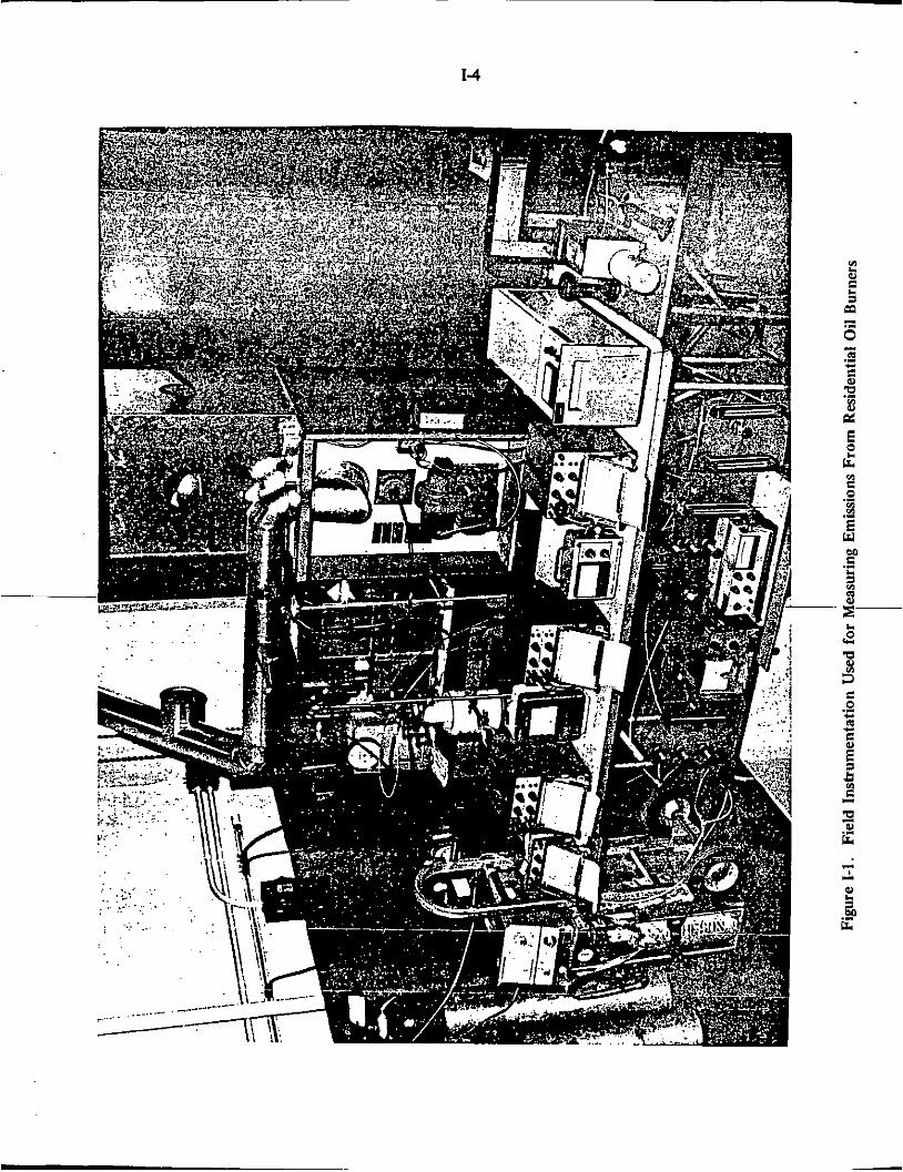
Figure 1-1 shows the emission measurement equipment being checked out on a residential burner-furnace unit in the BattelleColumbus laboratory prior to the field measurements. Figure 1-2 shows the instrumentation as set up in the field for measurements on a 150-hp Scotch boiler. I

Gaseous Measurements. In addition to the flue-gas analyses of oxygen and carbon dioxide needed to define the operating conditions in terms of excess-air level, the following gaseous pollutants were measured by continuous monitoring equipment sampling in the stack:


1-5

Figure 1-2. Field Instrumentation Used for Measuring Emissions From Commercial Boilers

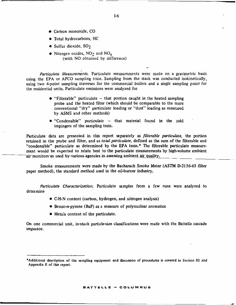
Carbon monoxide, CO

0 Total hydrocarbons, HC

0 Sulfur dioxide, SO2

Nitrogen oxides, NO2 and NOx (with NO obtained by difference)

Particulate Measurements. Particulate measurements were made on a gravimetric basis using the EPA or APCO sampling train. Sampling from the stack was conducted isokinetically, using two 4-point sampling traverses for the commercial boilers and a single sampling point for the residential units. Particulate emissions were analyzed for

“Filterable” particulate - that portion caught in the heated sampling probe and the heated fdter (which should be comparable to the more conventional “dry” particulate loading or “dust” loading as measured by ASME and other methods)

0 “Condensible” particulate - that material found in the cold impingers of the sampling train.

Particulate data are presented in this report separately as filterable porticulate, the portion retained in the probe and filter, and as total particulate, defmed as the sum of the filterable and “condensible” particulate as determined by the EPA train.* The filterable particulate measure ment would be expected to relate best to the particulate measurements by high-volume ambient air~monitors-as~used-byvarious agencies in-assessing ambient air quality. -

Smoke measurements were made by the Bacharach Smoke Meter (ASTM D2156-65 filter paper method), the standard method used in the oil-burner industry.

Particulate Characterization. Particulate samples from a few runs were analyzed to determine

0 C-H-N content (carbon, hydrogen, and nitrogen analysis)

0 Benzo-cu-pyrene (BaP) as a measure of polynuclear aromatics

0 Metals content of the particulate.

On one commercial unit, instack particlesize classifications were made with the Battelle cascade impactor.

‘Additional description of the sampling equipment and discussion of procedures is covered in Section 111 and Appendix E of this report.

E A T T E L L E - C O L U M E U S

SUMMARY OF RESULTS

Measurements on Residential Units

For the 20 oil-fired units in the as-foitnd conditions, the average smoke level was Number 4.2 on the Bacharach scale, with readings ranging from I to 8, and the average C 0 2 level was 7.9 percent. Adjustment by normal cleanup and service procedures to the tuned condition reduced the average smoke level to 1.6, with smoke readings ranging from 0.5 to 3; this was accomplished with an increase in the C 0 2 adjustment for some units and a decrease for others, but the average C 0 2 level for all tuned units remained unchanged at 7.9 percent.

The effect of tuning on gaseous and particulate emissions was variable, with emissions decreasing for some pollutants on some units and increasing for others; the most consistent pattern was that NO, emission levels generally increased on tuning. Emission levels for the cold-start condition were not significantly different from the as-found condition; the emissions measured with the reference fuel were not significantly different from the tuned condition, except lower SO2 levels reflected a lower fuel-sulfur content.

Figures 1-3 and 1-4 show the distribution of emission factors* and smoke levels measured on the residential units for the as-found and tuned conditions. It should be noted that two units were in poor condition and in obvious need of replacement; these units yielded oily smoke spots and gave CO, HC, and particulate emission factors that are completely out of the range of those for the remaining units. These units could be identified as needing replacement by a serviceman's inspection.

Table 1-1 shows the reduction in total pollutant emissions that were achieved by

1.. Identifying and replacing the two units in obviously poor condition

2. Completing Step 1 and, in addition, tuning the remaining units to low-smoke levels.

It can be seen for this selection of units that essentially the entire reduction of pollutant emissions was accomplished by replacing the units obviously in poor condition and that tuning of the remaining units effected only a minor reduction in emissions.

Emissions measured on one gas-fired furnace unit that was readjusted showed little change on tuning. In general, the emission factors for two gas-fired furnaces were lower than the mean for the oil equipment, but the HC levels with gas-fired units were nearly as high.

'Emission factors are based on fuel input and in this report are expressed in pounds of pollutant per 1000 gallons of fuel.

E A T T E L L E - C O L U M B U S

I

1-9

c .. .A - '5

c z

v) .a .- e 3

C 0

:'i E w

d) * 0

m c 0

E

Y 3

1-1 0

Table 1-1. Screening and Tuning of Units

Changed Mean Emissions by These Amounts(')

Smoke

co HC

Replacement Only

-63

-92

NO, +5

Filterable Particulate -21

Total Paniculate -38

Replacement Plus Tuning

-60%

-65

-93

+16

-14Ibl

-39

(a) Based on original sample of 20 units. Minus indicates emission reduction and plus indicates emission increase by percentage shown. Numerical averages of a l l data give 38 percent reduction of filterable particulate on tuning, but are believed to be distorted by lack of complete particulate data on one unit having high emissions in the as-found condition. Thus, the value shown here was calculated by assuming that emissions in the tuned condition and the as-found condition were identical for this unit.

( b )

Measurements on Commercial Boilers

Table 1-2 summarizes emission measurements on the oil-fired. commercial boilers for the baseline condition of 80 percent !oad and 12 percent C 0 2 nominal, setting. Also included is information on burner atomizer type and fuel properties. Boilers are listed in order of capacity within the categories of distillate fuel and residual fuel.

Emission levels for the boilen fixing distillate fuel were generally lower than for those firing residual fuel, as would be expected. The highest particulate emissions were measured with the heaviest residual fuels, SO2 emission levels increased in proportion to sulfur content of the fuel, and NOx emissions generally increased with increasing fuel-nitrogen content and increasing firing rate.

- The number of variables is so large (boiler sizes, burner types, fuel characteristics, etc.)

tha t i t is difficult to draw other significant conclusions as to the influence of single variables on emissions. However, some interesting trends are examined in Section VI1 of this report.


p ! " m $ !

" c ! - N

u? O -

N N

z z .o d

1-12

COMPARISON OF MEASUREMENTS WITH PUBLISHED EMISSION FACTORS

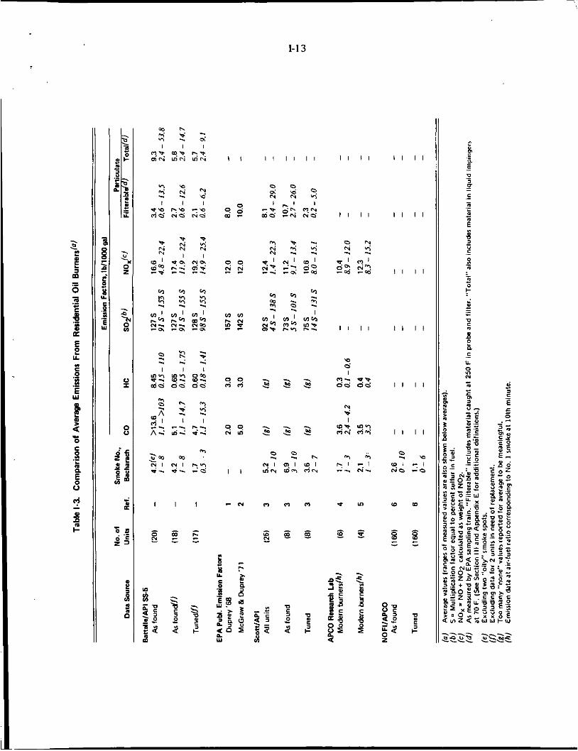
Tables 1-3 and 1-4 present a comparison of the emission factors from various sources, including

0 Data obtained in this investigation

0 Values listed in the various editions of Compilation of Air PoNutnnt

0 Data obtained from the earlier Scott/API investigation(3)

Data on residential units as measured by APC0(4,5)

0 Various other sources(6,7).

Emission Factors, published by EPA( 1,2)*

Both mean values and ranges of measured emission factors are listed.

In the summary tables, emission factors for SO2 are expressed in terms of pounds of SO2 per 1000 gallons fuel per percent sulfur content of the fuel, which allows for the adjustment of the emission factor for different fuel-sulfur levels. EPA’s published particulateemission factors are considered as “filterable” as no previous data are available on residential units and few data are available on commercial boilers using impingers in the particulate sampling train.

Emission Factors for Residential Units

For the residential units in this investigation, emission factors are summariZd-inTi6le 1-3 as follows:

0 As-found condition - mean for 20 units

As-found condition - mean for 18 units (excluding two units needing replacement)

Tuned condition - mean for 17 units (excluding the two units needing replacement and one unit that was not tuned).

Emission Factors for Commercial Boilers

For the commercial boilers, Table 1-4 shows a comparison of emission factors obtained in this study for the baseline condition, with factors from other sources. Comparisons are made separately for boilers fired with distillate and residual fuels.

‘References i itcd are listed 02 page 1-18.


1-1 3

I 1 I 1 I /

- _ \ * * t ?

I 1

I 1

I 1

I 1

I 1

I 1

I 1

1 1

I 1

I t

I 1

I 1

E e E '3 .E

U

0

W

- 0

i 2

B E 0

W

3

I 1 I l l 1

I 2s -0. I I I I

si I

Ki8 1 1 1 1

5 I

35 1 1 1 1

-. 2 1 1 I 1

. .~ , . .: . . - - '. . , I , . . . . -..... .......... 1-15 . . . I . ,

. . . . . . . . . . . ^ , . . . ... . . . -, .

. . . i

. . . ? . I

. . . . ._

..I . . . . . . . . .

CONCLUSIONS AND PERSPECTIVE

. . . ' The principal conclusions reached as' a result Gf this investigation on oil-fned equipmeit are as follows:

~ .. ' . . , -

.. i . . . . . . . . . .... . .

, . . . . . . . . . . . . . . . . . . . .~ . . . - ... . -

Residential Units . . : . . .

. . . . . . . . . . . . . . . I . . ,. , , < : . r . ' . . .

I .

';. 1: Emission. factors measured for residential units compare with other published .. . . . . . . ' I data and emission factors as follows: ~.

. .

- , - . . . . : ~ . - . . . . . . .

CO - Higher than values reported for other field and lab measure- . ments and about equal to the value published by EPA in

. . . . .

. . .. .,. , . . . . . . - . . - . 1971

HC - Higher than values reported for other field and lab measurements and about 80 percent lower than EPA's published value

. .

SO2 - Slightly-higher than values reported for other field measurements. Lower than EPA's published value and emission factors calculated from sulfur content of the fuel. (SO2 was generally proportional to sulfur content.)

,

NO,- Fifty percent higher than the reported values for other field and lab measurements and EPA's published value (although all NO, measurements for residential units in this investigation were below 100 ppm)

. .

Filterable particulate - Emission factors for the as-found condition are only about one-third of values reported for other field measurements and EPA's published values. Emission factors

Total

for the tuned condition were about the same as values reported for other field measurements and about one-fourth of EPA's published values. (Filterable particulate averaged about 40 percent of total particulate emissions.)

particulate - No previous data on residential units were found and EPA has no comparable published value.

2. Screening and tuning of the residential oil burners significantly reduced total pollutant emissions of the entire sample of 20 oil burners by identifying two units in need of replacerent. These two units were contributing 63 percent of the CO, 92 percent of the HC, and 38 percent of the total particulate emitted

. by the entire sample of 20 units. Tuning did not significantly reduce average .. pollutant emissions for the remaining 18 units;although average smoke number

was reduced from above No. 4 to below No. .2. . . . . . .

. . . . . . . .


. . . .

. . . . ., _ . .

(' with other published emission factors as follows (No other field or lab data &e found for distillate-fired boilers.): . . . . .

- : . . . . . . . . - . . . c . . '

tiy higher than the value published by EPA k 1968 higher than the value published

..L. . . . . . 1 ....... ,:.?'~~'.:.< . than EPA's pubhshed h u e ' '

.............. . . . . - .......... . . . .; . . . . . . . . . . . . . . . . . . . . . . . . . .

. . . . . . . . . . . . ., ;- . , . . . . . . .

. .

. . . . .

. . . . ..SO2 - Equal to EPA's published value and generally proportional . . . . . . . .... ~ .... ?.. . . .

. . . . . ' . . . . . . . . . . . . . . . . . . . . . . . . . . . . . . . . . . . . . . . . .

. . . . . I . to fuel sulfur content . , '

. . . . . . . . . . . . . . - . . .. . . , .

- . .,. .

i . . . . . . .: . 'NO, - Significantly lower than EPA's published value . . . . . . . . . . . . . . . . - . . . . . . . . . . . . . . . . . . . ~ . . ..., . . . ". . - . . . .

~

~ . .

. . ' ~ Filterable particulate - Only about oneeighth 'of EPA's published value for particulate emissions

. . Total particulate' - Although total particulate is not considered

comparable to particulate as reported by EPA, the emission .. factor for total particulate as determined in this study is

. . . about equal to EPA's published value for particulate ,

. . ~' emissions. . .

4. Emission factors m e a s u r ~ d - f o ~ i e s i d u a I ; f u e l ~ ~ ~ e d - c o ~ ~ c ~ l - ~ ~ e r s - c o m p a r e with other published data and emission factors as follows:

. . CO - Within the range of values reported for other field measurements, twice the value reported by EPA in 1968, and much higher than the value reported by EPA in 1971

HC - One-fourth of values reported for other field measurements .

SO2 I Equal io EPA's published value and generally proportional . . to fuel sulfur content (cannot be directly compared with

. : and less than one-tenth of EPA's published value . . . . . . . . . .

. . . . . . . \ _ . . . .-existing field data, as sulfur levels of fuels fired in the . . .

. . earlier trials were not reported) , . .. . .

. . . . . . NO, - Significantly higher than values reported for other field measurements and within the range of EPA's published values

.. . . .. -

. . . . Filterable 'particulate - Equal to value reported for one field study . ' .and one-half the value reported for another field study and . . .. . . .

. . . . .

. .

. . . , , ' . . ; . 1;- .. EPA's published value

. ' :.

. . . . . . . . . . . . . . . . . . . -

' .Total particulate - Slightly lower than the value reported for one

. value). .

. . - . . _ . . . . . 1: " previous field study (EPA has not published a comparable

. .

. .


" . . . . .fuel and by firing rate, although other factors may also have influenced

. . . ' emission levels. The .trend of NO, levels generally @creased with fuel nitrogen ': and with f ~ n g rate, the lower limit of measured values inkeasing as the f h g

. . . . . . . . . . .

. ' ~ .- , . .."T i:..

. .... . . . . . . . . . . . . . . . . <',;:', . . . . . '_ . % 1 . <.'.. ~ .. . . - . . . . . . . . . . . . . . . . . . . . . .

..- .:: . . , , ..I . - : rate increased.

. . .I ,. . - . . . , . . .. I .~ . . . . - . . . . I

: I .6. 'HC e m k o k measured in .this investimtion were v e 4 low -' freauentlv lower . . . , . - .. : t hm ' the background level a t the measurement location. . ' . . .

.. .. . . . . . ' I . . . . . j , . - ,: . . . - . . - .;. s . -

' 7. Bacharach smoke number'at steady-state conditions was not a good measure of

. residential units operating on a cyclic basis and commercial bailers operating .. . . . ..integrated particulate ekssions on a weight basis. This was true for both

. . . .

. . . . . . . . . . . . . . . .. . . on a steady-state basis. . .

. . -.

'In drawing conclusions, the wide. range in emission factors from field measurements must be recognized. Emission factors for oil-fired 'equipment vary over a significant > c range, and these variations are related partly to differences in the nature of the oil-burning equipment (size and type) and partly to the nature of the fuel. The variations notwithstanding, until more extensive data become available, the emission factors obtained in this investigation of a limited equipment sample offer a reasonable basis for assessing emissions from oil-fired equipment for space heating.

. . . . . . .

. . . . . . ., . . . . . .

. . . .

- .

. . . . . . . . - . . , . .

. E A T T E L L E - C O L U M E U S

. . . .

. . . . . . . ... .. . . . . . .... . . . . . . . c . . . . . . . .

~ . . I. . ..

. . . . .

&.

. .

. . . . . . . .

, ’ . .

. . . . ,

- . .

. . .

, , . . .* . .

. . . . -

REFERENCES FOR SUMMARY TABLES

1. Duprey, R. L., “Compilation of Air Pollutant Emission Factors”; National Center for Air . . . . . . .

: Pollution Control,’ U.S. Public Health Service Publication No. 999-AP-42, 1968, p 7.

. . . . . . . . . ‘2. McGraw, M. J., A d Duprey, R: L.,. “Compiiation of Air Pollution Emission Factors”,

Preliminary Document, Environmental Protection Agency, April, 1971, p 10.

3. Burroughs, L. C., “Air Pollution by.Oilburners - Measurable but Insignificant”, Fuel Oil and Oil Heat, June, 1963, pp 43-46 +.

4. ‘Howekamp, D. P., and Hooper, M. H., “Effects of Combustion-Improving Devices on Air Pollutant Emissions from Residential Oil-Fired Furnaces”, AFCA Paper No. 70-45, 1970, 33 PP. . .

5. Howekamp, D. P., “Flame Retention - Effects on ‘Air Pollution”, Presented at 9th Annual Convention, NOFI, Atlantic City, New Jersey, June 9-11, 1970,.10 pp.

6. Bunyard, F. L., and Copeland, J. O., “Soiling Characteristics and Performance of Domestic and Commercial Oil Burning Units”, NAPCA, January 28, 1968.

. .

7. Scott Research ‘hboratories, Inc., reports on NCAPC Contracts/No. PH 27-00154 and PH . . . . . . . . . . . . . . . .

. .

. . . . . . . . I . .

. . . . . . . . . . . . . . . . . -~

22-68-125, 1968. ,, . . . .

. .

,; ~. - . . . . .

. .

. . . . . . . I .

. .

, .

, .

. . . .

- . .

. . . . . . . . . . . . . . . . . . . . . . . . . . . . . . . . . . .

. . . . . . . . . . . . . . . . . . . . .

. . . . ,

. . . ’ ..

. . - . . . .

. . . 1 .

-

. . . .

. . :. . . .

.. , . . :_

. . . . . .. . . . ~ .

. . I . . .

. . . .

. . .. , ,

. . . . . . . .

. . . . . . .. .. . . . . . .

. . ’ . . . .

. . . . . .


11. SCOPE OF EQUIPMENT COVERED IN THE INVESTIGATION

The scope of equipment included in this investigation extended from 20 oil-fired residential units and wiiter heaters, with firing rates from 0.5 to 3.5 gph, to 7 oil-fired commercial boilers in the 60 to 350 HP range firing from 7.6 to 104 gph. Two gas-fired residential furnaces and one gas-fired commercial boiler were included for comparative purposes.

Basis for Selection of Equipment

The oil-burning equipment installations selected for this program were intended to be representative of the population of equipment in service considering such factors as:

Classes of equipment o r application - residential or commercial

Installation type - matched unit (burner-boiler unit or burner-furnace unit) or

conversion burner

Burner type - atomizing type, combustion head, etc.

Capacity or firing rate

Fuel grade

Heating system type - hot water, steam, or warm air

Age of installation.

Obviously, within the limits of a program of this size, it was not possible to include a large number of units in each category. However, an attempt was made to include a distribution of oil-fired units similar to the distribution of units now in service.

As a basis for this selection, various sources of statistics on oil-fired equipment were consulted including Fueloil & Oil Heat magazine, the National Oil Fuel Institute, and the American Boiler Manufacturers Association (ABMA). This information, combined with the experience background of the project team, was used in establishing a suitable mix of units. The Battelle-Columbus recommendations as to the general equipment mix were then examined and approved by the API SS-5 Task Force.


-

11-2

RESIDENTIAL UNITS

Selection of Equipment Mix and Individual Units

Table 11-1 outlines the types of equipment included in the residential equipment mix and shows the number of units in each type included in the investigation.

Background data used in establishing the mix of domestic equipment are shown in Appendix A. These data represent statistics on equipment sales and, to some extent, units in service. No direct statistical data are available covering detailed categories of equipment now in service on a national basis; however, the data in Table A-2 can be used as a rough guide to the population of burner types by assuming that the present population is closer to the recent sales distribution than to the prewar distribution. High-pressure gun-type burners are clearly the dominant burner type for residential heating.

Selection of the individual residential field units was made with the assistance of Consultant W. H. Axtman and with the aid of a qualified oil-burner servicing organization. The servicing organization supplied a skilled serviceman to tune or adjust the burners following the initial measurements. The majority of the units investigated were selected from the service contract files of the organization, and the initial contact with the homeowner was made by the servicing organization.

Desccption of Residential Units

Table 11-2 shows the number designation used to identify emission data elsewhere in this report for the specific residential units selected. This table also includes a brief identification of burner type, firing rate, heating system type, and burner and system age - including whether the installation is ( I ) a “matched” factorydesigned burner-furnace or burner-boiler unit or (2) a “conversion” installation where the burner has been added in the field to a basic furnace or boiler; possibly originally coal fired. (Nearly all furnaces and boilers being installed today are matched units.)

Twenty of the units were oil fired and two of the units were gas fired. Eighteen of the oil-fired field units were high-pressure gun-type, four with flame-retention heads and two with Shell combustion heads. One of the units was a low-pressure burner and one was a vertical rotary wall-flame burner.

Four of the oil-fired field units were warm-air furnaces, fifteen were water or steam boilers, and one was a tank-type water heater. Seven of the twenty units investigated were conversion units. The ages of the burners and heating systems ranged from 1 to over 30 years.

An additional unit, identified as “0”, was a new residential oil-fired furnace which was set up in the laboratory a t BatteUe-Columbus for the calibration and checkout of instruments, UmpLng procedures, and the operating cycle timing.

A summary of the tuning procedures required to achieve acceptable smoke levels for each unit is contained in Appendix C.


11-3

Table 11-1. M i x of 22 Residential Installations Sampled

(Units Unit i in in

Subclan) clau

DISTILLATE OIL BURNERS - 20

a Modern furnace-burner matched units, pressure. atomizing burner 3

a Modern boiler-burner matched units, preaure- atomizing burners 7

- Steel boiler (2)

- Cart iron boiler (6) -Conventional burner (2) - Flame-retention head (2) - New, 3450 rpm burner (1)

a Modern water heater-burner matched units

Older conversion burners in cast4ron boilers

- High-pressure gun type -Conventional burner (3) - Flame.retention head (1) -Shell head (2)

- Vertical rotary wall flame

a Older matched unit, low-pressure type

a Conversion. cast-iron warm-air furnace

1

7

NATURAL GAS BURNERS - 2

Modern burner.furnace matched units 2

-Sectional furnace, multiport ribbon (1) - Drum-type furnace, multiport burner (1)

11-4

Table 11-2. Description of Residential Units

Firing Rate (b), Estimated Age, y n

Unit Burner Type (0) wh HeatingSystem Type IC) Burner System

1

2

3

4

5

6

7

8

9

10

11

12

13

14

15

16

17

18

19

20

21

22

0

Hi-press gun

Hi-press gun

Hi.press gun

Hi.press gun

Hi.press gun

Hi~press gun, flame.ret. head

Hi.press gun, flame-ret. head

Hbpress gun. flame-ret. head

Hi-press gun

Hi-press gun

Hi-press gun

Hi-press gun

.Hi.press gun, Shell comb. head

Hi-press gun

Hi-press gun, flame-ret. Gd-/d)-

Hi-press gun. Shell comb. head

Hi-press gun

Hi-press gun

Low pressure

Vertical rotary

Sectional gas burner

Multiport gas burner

Hi-press gun

1.35

1 .oo 3.00

1.25

1.25

1.35

2.50

1.50

3.25

2.50

0.50

1 .oo 1.25

1.35

3.50

1.75

2.50

1.35

2.10

0.58fe)

137 lf)

- - - _

1 50 If) 1 .oQ

Steel-boiler unit, water

Horizontal steel forced-air furnace unit

Steel-boiler unit, water

CI gravity warm-air furnace, conversion

CI boiler, conversion, water

CI boiler unit. water

CI boiler unit, water



CI boiler, conversion, steam

Storage-type water heater

Steel forced-air furnace unit

CI boiler, conversion, water


C l - b % i l f i i t , water


CI boiler unit, steam

Steel forcedair furnace unit

Steel boiler unit, steam


Gas-fired, forced-air sectional furnace

Gas-fired, forced-air drum furnace

Steel forced-air furnace unit

~

12

13

9

>30

15

1

12

1

1

15

1

3

4

15

-1-

1

3

3

>20

>20

5

11

<1

12

13

9

>30

15

1

12

1

1

>30

1

3

15

>20

1

8

15

3

>20

>20

5

11

<1

(a) (b ) IC)

(d) (e) Firing rate, tuned condition.

If)

Burner atomizing type: special combustion heads noted, including flame-retention heads. Nominal firing rate or nozzle capacity as found, gph.

"Unit" describes "matched" burner-furnace or burner-boiler units engineered by the manufacturer. CI denotes cast.iron construction.

High-speed burner, 3450-rpm fan motor.

Gas burner input in lo3 Btu/hr.

11-5

COMMERCIAL BOILERS

Selection of Equipment Mix and Individual Units .

Table 11-3 outlines the mix of commercial boilers covered in the investigation as representative of commercial heating boilers in the field. The selection of this equipment mix was made by the Battelle-Columbus project team after discussions with the ABMA Commercial- Industrial Air Pollution Committee and Consultant W. H. Axtman.

Table 11-3. Mix of Eight Commercial Boilers Sampled

Number of Units

Boiler Type

Scotch

Firebox firetube

Burner Type

Air atomizing

Pressure atomizing

Rotary atomizing

Natural gada)

Fuel

No. 2 oil

No. 4 & 5 oils

No. 6 oil

Natural gasla)

7

1

~~

(a) Natural gas was fired in one boiler equipped for duabfuel operation and recorded as a separate boiler for identifica. tion of data.

Background statistics from ABMA are presented in Appendix A on commercial-industrial burners showing the distribution of sales by burner atomizing type and by fuel class.

Two types of boilers, modified package Scotch and fiiebox, were identified as having furnace volumes and operating characteristics analogous to most other types. These two types also represent a large portion of the commercial boiler market in recent years.

B A T T E L L E - C O L U M E U S

11-6 i l I Burner selection was determined by an analysis similar to that used for selecting

residential units. However, particular attention was given to burners in the 400,000 to , 25,000,000 Btuh range. Air-atomizing burners accounted for 46 percent of the burners sold in the size range of interest. Consequently, four burners of this type were selected. Pressure atomizing burners accounted for 38 percent of the commercial sales in 1969, therefore two burners of this type were included. Although rotary cup atomizing burners accounted for less than 7 percent of sales, the number of these burners was significantly higher in past years. Since many burners of this type remain in use, a rotary burner was included in the equipment mix. As steam-atomizing burners are not common in this size range, none were included in the equipment mix selected for this investigation.

Another criterion used in the selection of commercial equipment was fuel grade. In 1969, 37 percent of the commercial boilers sold were operating on No. 2 fuel oil and 63 percent on residual oil (Nos. 4, 5, and 6). Therefore, two boilers were selected for No. 2 oil, two for No. 4, two for No. 5, and one for No. 6 oil. In addition, Boiler C1002, using an air-atomizing burner, was investigated while firing three residual oils of different sulfur contents; the three oils are representative of fuels in current use in various geographic locations. One power-type gas burner was included in the equipment mix for comparative purposes.

The final criterion for boiler selection was method of combustion control or operating mode. Because modulating type control is most commonly used (especially for larger boilers) and is also required by several regulatory authorities, five boilers having this type of control were included. The remaining boilers had on/off (or on/off with low-fire start) controls.

These boiler selections are believed to be generally representative of boilers in the field today, within the limits placed by the size of the sample.

_ _ For purposes of this investigation, it was important to select boilers for which load could

be controlled at a desired level for extended periods to provide stable conditions for emission measurements. This requirement was met, through the cooperation of ABMA, by choice of equipment installed as house boilers or test boilers in plants of boiler manufacturers. In addition, competent personnel already familiar with the specific equipment were available to adjust the boilers to the desired operating conditions. Normally, these boilers were in day-to-day operation to supply steam, to provide service training, or a burner test facility for the manufacturing plants. These boilers did not appear to have received any better service attention than would be reasonably typical of similar boilers in commercial or industrial applications.

Description of Commercial Units

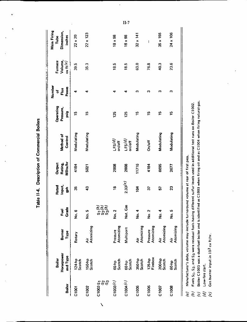
Table 11-4 shows the number designation for each commercial boiler, with identification of boiler type and size, burner type, nominal fuel grade, and other descriptive data.

Boilers C1001, C1002, and C1003 were typical “house boilers”, C1005, C1006, and C1007 were burner test boilers, and C1008 was a laboratory installation. One boiler was equipped for dual-fuel operation and was fired with No. 2 fuel oil identified as Boiler C1003 and with natural gas as C1004.

~ A T T E L L E - C O L U M ~ U ~

11-7 ,o

E

m m 0 - .- - m a,

.- e E E s r 0

e -

P m E Z

L o o n o

w m

z z 0 0

cn C N ._ .-

4- $ E 0 .= s a a a

QC PI:

0 0 0 N U m u - v ) - v )

6 s g s

- N 0 0

0 0 0 0 L

\

111. FIELD INVESTIGATION AND PROCEDURES

The principal effort in this investigation was devoted to field measurements of emissions and was conducted during the heating season of 1970-71. The measurements were made by a three-man field team, supported by other Battelle-Columbus staff and a consultant.

Measurements on residential heating units were started in February, 1971, and, except for two follow-up runs, were completed in April, 1971. The investigation of each residential unit required from 2 to 3 days, including instrument setup and measurements under the test conditions.

Commercial boiler measurements were conducted in April and May, 1971, each boiler requiring approximately 3 to 5 days depending on conditions and fuels run.

RESIDENTIAL UNITS

Burner Conditions Investigated

Emissions from residential units were monitored under four sets of burner conditions:

“Cold-start condition”, measurements with the as-found burner adjustment during the first IO-minute run (after >60-minute off period)

“As found condition” of burner adjustment, measurements made after several repeated cycles of 10 minutes on and 20 minutes off.

“Tuned condition”, only if the performance of the as-found conditions warranted adjustment (smoke above No. I), measurements after several repeated cycles.

“Reference fuel run”, generally run at the tuned adjustments after several repeated cycles to provide a baseline for comparison of units.

C -

- A

- T

- R

The letter designations (C_, ,4, 1, and - R) are used elsewhere in this report to key the condition of the measurements.

Definition of Tuned Condition

Experience on the first five residential units indicated some variability among servicemen in their criteria for a well-tuned unit. For the other units, the tuned condition was specifically d e f i e d as the best adjustment (in terms of the smoke-CO2 relationship) that could be achieved by a skilled serviceman with normal cleanup, nozzle replacement, simple sealing, and adjustment procedures with the benefit of field instruments. It did not include major repairs, modernization, or replacement of major parts that would require s F i a l charges to the homeowner (e.g., replacement of a combustion chamber). Further details of the adjustment procedure are presented in Appendix C.

111-2

14

0 4

Legend

0 As-found 0 Tuned + No change on tuning

CO, in Flue Gas, percent

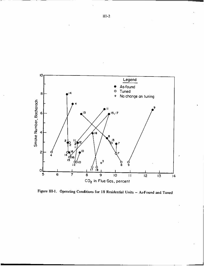
Figure 111-1. Operating Conditions for 18 Residential Units - As-Found and Tuned

111-3 .3

Operating Conditions. Figure 111-1 shows the smoke and CO2 level of 18 residential units, with unit numbers identified.* In those cases where the unit was tuned, the lines connect the as-found condition and the tuned condition. The CO2 levels were generally reduced in tuning to lower smoke, even though 4 units were tuned to higher C02; the nozzle was replaced in all 4 of these units as part of the tuning procedure.

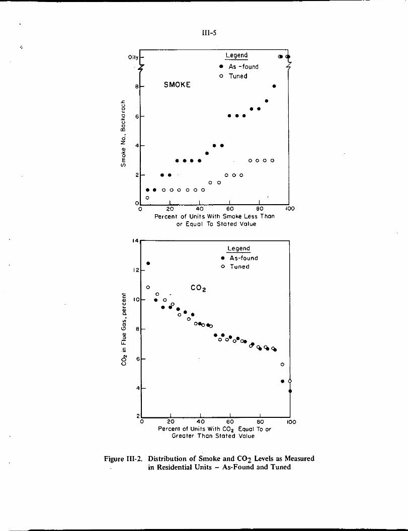
Figure 111-2 shows the distribution of smoke and C02 levels for the residential units. These data represent all 20 units, 18 of which were tuned. In the as-found condition, 55 percect of the units operated with a No. 4 smoke or less, and 20 percent with No. 2 smoke or less. In the tuned condition, all of the units except Units 5 and 20 were capable of operating at No. 3 smoke or less, and 70 percent of the units operated with No. 2 smoke or less. The mean smoke level for 18 units as-found was 4.2 and for 17 units tuned was I .6.

While changes in C02 were affected by 'tuning some units, little overall difference in distribution was noted and the mean was 7.9 percent both as-found and tuned.

Complete data on operating conditions (for the cold-stat, as-found, tuned, and reference- fuel runs) are tabulated in Section IV.

Cycle Selection for Emission Measurements

A uniform operating cycle was used for all the residential units to provide a consistent operating mode for emission measurements. After consideration of the various factors involved, a cycle of 10 minutes on and 20 minutes off was chosen. The rationale of the fixed firing cycle was based on the following criteria.

I . The resulting emission data should be capable of comparison between installations on a common basis, independent of the effects of outdoor weather on operating modes.

2. The field program should not be seriously delayed or limited by weather during the normal heating season. (Attempts at making measurements during normal control cycles encountered very erratic timing.)

3. Multiple cycles of controlled operation should allow the burner and combustion chamber to reach a repeatable thermal condition.

4. The on-period should be long enough to allow for the response time of monitoring equipment and allow measurements to reach equilibrium.

*Two of the 20 residential oil-fired units (No. 5 and 20) yielded yellow smoke spots with traces of unburned oil such that smoke readings were not meaningful and could not be averaged with other data. These units were in such poor repair that performance was completely unsatisfactory and proper adjustments could not be achieved without major replacement beyond that planned for this investigation; these units would be recognized as needing replacement by a competent serviceman. Unit 6 had been tuned only three weeks before the measurements were made and was not considered t o need additional tuning; these data are included in averages and summaries for as-found and tuned units. Unit 19 was not tuned due to difficulties in adjustment.


111-4

5. A IO-minute on-time is longer than will be encountered with direct burner control by a modern heat-anticipating room thermostat, where 5 cycles per hour at 50 percent on-time is the design basis,@) but may be shorter than encountered for a hydronic system controlled by the temperature of a water circuit or by steam pressure. A choice of IO minutes is a reasonable compromise.

6. The 113 operating time or “load” of the 10-minutesun/20- minutes-off cycle represents a reasonable average load condition during the colder part of a heating season.(9) (When warm weather was encountered, the heating load was increased by opening doors or by drawing water from a domestic hot-water hookup.)

Similar considerations have led other investigators to choose the l@minutes- on/2&minutes-off cycle as a basis for their studies. For example, Mobil Oil Corporation(9) uses this cycle in various burner and fuel evaluation tests, and EPA investigators have used this cycle as a standard for laboratory programs to simulate operation of residential equipment.(4,10)

I t can be argued that additional investigation should be made of the effect of cycle. However, for purposes of this limited field investigation, the use of the I@minutes- on/?@minutes-off cycle was selected to be a practical compromise.

Timing of Sarnphg. Measurement of gaseous emissions were made continuously over the IO-minute-on period of the cycle. However, due to time lag in the instrumentation, S02, NO, and NO2 readings required nearly IO minutes to reach equilibrium; hence, these emission factors were calculated on the basis of the 10th minute reading. Emission factors for CO and HC were based on time-average values over the l@minute-on period, including peaks at starting but not including peaks at shutdown - when the combustion air flow was diminished and recorded concentrations were not meaningful. (Appendix D contains a comparison of the 5th minute, 10th minute, and average ppm values for CO and HC.)

Bacharach smoke measurements were made at the midpoint of the firing cycle (5 minutes) and, in most instances, at I and 9 minutes. The smoke numbers reported are for the 5-minute point in the cycle.

Particulate sampling was conducted during the 1 O-minute+n period of the burner for five or six consecutive cycles after the initial cold-start cycle. The particulate sampler was started just before burner startup and continued to just beyond shutdown.

~

(8) Private communication: to D. W. Locklin, Battelle-Columbus, from Norton Saude, Honeywell, Inc. (February 26, 1971).

(9) m a t e communication: to D. W. Locklin, BattelleColumbus, from W. F. Herpeter, Mobil Oil Corporation (April 22, 1971).

(IO) Wasser, I. H., Hangebrauck, R. P., and Schwartz, A. I., “Effects of Air-Fuel Stoichiometry on Air Pollutant Emissions from an Oil-Fired Test Furnace”, Journal of Air Pollution Control Association, Vol 18, No. 5, pp 332-337 (May: 1968).

111-5

Oily Legend

AS -found 0 Tuned

SMOKE

d = 4 w 1

2 m t ul

2t

a 0 . ...

0 . . .... 0 0 0 0

0 . 0 0 0 0 0

..ooo 0 0 0 0

0 I I I I 0 20 40 60 80

Percent of Units With Smoke Less Than or Equal To Stated Value

L E al

al Y a VI 0 a al a e c .-

0" V

Legend

8 As-found 0 Tuned

D O

0 . 2 0 20 40 60 80

Percent of Units With COP Equal To or Greater Than Stated Value

Figure 111-2. Distribution of Smoke and C02 Levels as Measured in Residential Units - As-Found and Tuned

111-6

Reference Fuel

To obtain a baseline or reference for the variety of burner units tested, gaseous emissions were measured for each residential unit for several cycles while firing a reference fuel. This reference fuel was selected as a high-quality NO. 2 hydrotreated fuel and was run after the units had been tuned.

Properties of all fuels used in this investigation are tabulated in Appendix B, Tables B-I and 8-2.

Gar-Fired Units

Emission measurements were made on two gas-fired residential furnaces in the Columbus, Ohio, area. Measurements were made for the cold-start condition and the as-found condition (warm). Unit 21 was tuned by a serviceman and measurements then were made for the tuned condition. Unit 22 was not tuned.

These gas-fired units did not have high-temperature, high-thermal-capacity combustion chambers and, therefore, the data from coldstart and warmstart runs in the as-found condition were essentially identical. As tuning was limited to adjusting the primary air setting, it did not significantly affect emissions.

Both of the gas-fired units had built-in draft diverters. Due to the difficulty of achieving representative sampling from the individual flue sections upstream of the down-draft diverter, measurements were made downstream of the diverter and, therefore, included dilution air. While the ppm concentrations of pollutants are affected by this diIution, emission factors based on fuel input are not affected. .

COMMERCIAL BOILERS

The instrumentation technique and 'emission measurements employed for the commercial units were similar to those used for the residential units. However, the conditions under which the measurements were made were quite different.

The commercial boilers were all sampled in the as-found condition; no cleaning (except for the exhaust stack) or other servicing of the units was done prior to measurements. Wherever practical, the exhaust stacks were thoroughly cleaned prior to sampling to minimize collection of previously deposited material during particulate sampling.

Load Conditions

Emission data from the commercial units were obtained under steady-state firing conditions at four different load levels


111-7

80 percent of rated load and 12 percent C02

An intermediate load

Normal low-fire setting

Typical load - the generally accepted or established firing rate for the installation.

To assure a steadystate condition, the boilers were operated for at least 30 minutes a t each load setting before sampling was started. Particulate samples were obtained at two loads: 80 percent load and low fire. Gaseous emission measurements were obtained at all four loads.

After discussions with the ABMA Air Pollution Committee and the API Task Force, a baseline operating condition of 12 percent C 0 2 and 80 percent load was established. No other adjustments were made after the air-fuel proportioning linkage was adjusted to this setting, thus, the air-fuel ratios at the low and intermediate loads were controlled by the linkage. The run at the typical operating condition for the boiler was made at the C02 level at which the boiler is generally fired for the particular installation.

In addition to the house fuel, three residual fuel oils with different sulfur levels were examined in one of the commercial boilers at the 80 percent load setting. These fuels were typical of the current commercially available East Coast fuels at these sulfur levels. Their compositions and properties were quite different (see Tables B-3 and B-4) as a result of the r e f i n g or blending processes used to lower the sulfur levels t o meet regulations in various localities.

INSTRUMENTATION

Prior to measurements in the field, all the equipment and instruments required for the investigation were standardized and checked out in several runs on a residential oil-fired furnace in the Battelle-Columbus laboratory. Sampling procedures and test sequences were also checked out at this time.

An established set of operational procedures was routinely followed for each unit investigated. Stack gdses were sampled and supplied directly to continuous monitoring equipment set up alongside the heating unit.

Gaseous Emissions and Smoke Measurements

Measurements were made of the following stack emissions under various conditions of operation using the methods noted as follows. (Details of instrumentation and measurement procedures are described in Appendices D and E.)


111-8

Emission Measurement Method

Smoke . . . . . . . . . Bacharach (and Von Brand for monitoring) CO2 . . . . . . . . . . NDIR (nondispersive infrared) and Fyrite 0 2 . . . . . . . . . . Amperometric and Fyrite CO . . . . . . . . . . NDIR Hydrocarbons (total) , . . Flame ionization SO2 . . . . . . . . . . Dry electrochemical NO,. . . . . . . . . . Dry and wet electrochemical N02. . . . . . . . . . Wet electrochemical Particulate . . . . . . . EPA (AFCO) sampling train.

In addition to these measurements, other combustion conditions were measured, including:

Draft, overfire and stack

Firing rate, measured volumetrically

Stack temperature, measured in the flue at the particulate sampling location.

For the residential gas-fued units, measurements were taken downstream of the draft diverter because of the difficulty in obtaining representative sampling upstream of this location. The bleed air entering through the diverter affected ppm levels but not emission factors.

Particulate Sampling

Particulate samples were collected using the EPA (APCO) sampling rig.(11,12) This rig was developed by the Environmental Protection Agency for sampling particulate emissions from incinerators in accord with the EPA definition of particulate matter as alI solids and condensible materials which are liquid at standard conditions of I atmosphere and 70 F, excepting uncom- bined warer(l3).

A special feature of this sampling train is the inclusion of two water impingers or bubblers (at 70 F) downstream of the filter. This train is described in Appendix E. The impingers are intended to collect any condensible material (at 70 F) that would exist as vapor at filter temperature and, thus, pass through the filter and any solid particulate that passes through the filter. There is concern that reactions occur in the impinger to generate material that is included in the weight measurement of particulate, even though the material does not exist as particulate either in the flue gas or in the atmosphere. Battelle-Columbus is currently investi- gating the composition of particulate from fossil-fuel-fied equipment as sampled with this train.*

~~

( I 1) “Specifications for Incinerator Testing at Federal Facilities”, US. Dept. of Health, Education, and Welfare, Public Health Service, Bureau of Disease Revention and Environmental Control, National Center for Air Pollution Control, October, 1967, 34 pp.

(12) “Standards of Performance for New Stationary Sources”, Federal Register, Vol. 36, No. 139, Part 11, pp 15704-15722, August 17, 1971.

(13) NAPCA RFP No. CPA 7ONeg 218, Scope of Work, p I ( l 9 7 1 ) .

*EPA Contract No. EHSD 71-29, “The Chemical Composition of Particulate Air Pollutants from Fossil Fuel Combustion Sources”.


111-9

To' insure that the most meaningful information was obtained from the particulate samples collected on this API investigation, the probe wash, the filter catch, and the impinger wash were treated separately and particulate weights recorded on each. In this report, particulate data are reported as filterable (including the probe and filter catches) and total (combining the filterable and the material found in the water impingers). However, it should be pointed out that even the filterable catch obtained using the EPA sampling train may not be directly comparable to the particulate catch obtained using other sampling trains, because the EPA procedure requires washing the probe and most other procedures require dry brushing to clean the probe. The uncertainty comes in the drying of the probe wash, as discussed further in Appendix E.

* * * * *

Presentation of Results

Data obtained using these measurement methods are presented and discussed in the following sections:

Residential Units

Section IV

Section V

Emissions from Residential Units

Discussion of Findings - Residential Units

Commercial Boilers

Section VI

Section VI1

Emissions from Commercial Boilers

Discussion of Findings - Commercial Boilers


1v- I

IV. EMISSIONS FROM RESIDENTIAL UNITS

EMISSION MEASUREMENTS

Emission data were obtained for CO, total HC, S 0 2 , NO, NO2, and particulate (filterable and total). Gaseous emissions as measured in ppm and particulate loadings in grains per standard cubic foot are presented in this section, followed by calculated emission facfors in terms of Ibs per 1000 gallons of fuel fired for oil and Ibs per million cubic feet for gas.

Gaseous-Emission Profiles

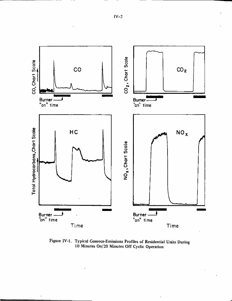
It is well recognized that a time delay exists in reaching steady state during the firing cycle. Using the 1 O-minutes-on/20-minutes-off cycle, it was possible to observe transients with the fast-responding monitoring equipment for C 0 2 , 0 2 , CO, and HC. Figure IV-1 portrays a complete on-off cycle for the C02, CO, HC, and NO, recordings. In the case of NO, NO,, and SO2 monitoring, response time of the instruments to full-scale reading was too slow to fully portray on-off cycle effects; however, the apparent increase in NO, with burner on time can be attributed partly to the increasing combustion-chamber temperature.

In the case of CO and HC, a marked increase (peak) in emission concentrations was observed as the burner started and as the burner shut off. This increase may be related to several factors. At the start of the “on” cycle there may be (1) slow buildup in air flow as the fuel is injected into the combustion chamber, (2) delayed ignition, or (3) incomplete combustion. At the end of the cycle, the peak is probably related mainly to delay in complete oil shutoff.

The question arises as to the influence of the peak in the average emission during the entire on period of the cycle. Table D-2* presents the 5th-minute and 10th-minute readings and the dose averages for CO and HC. (The dosage is defined as the area under the ppm vs. time

m x m i n - - curve during the “on” cycle. The dose average is this area divided by IO minutes, i.e., pp

dose average.) In general, the 10th-minute HC reading is greater than 90 percent of the dose-average reading over the IO-minute on period. For CO, the difference between the 10th- minute and dose average values is greater. Reasons for the greater deviations are not apparent. For NO, and S02, the 10th-minute readings at the end of the “on” cycle, Le., just before shutoff, were used for emission factor calculations. However, for CO and HC, the dose average values were used for emission factor calculations.

10

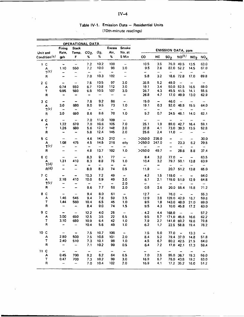
Gaseous-Emission Data

Table IV-1 lists the gaseousemission data measured at the 10th-minute point in the “on” cycle for the five gaseous species.” Also shown are levels of C 0 2 and 0 2 , excess air, Bacharach Smoke Number, firing rate, and stack temperature (at the sampling point) for the conditions run on each residential unit.

‘See Appendix D. **Examination of Table IV-l reveals that NO2 emission measurements for Units 1 through 15 were generally higher

than expected and higher than measurements for the remainder ofunits. Examination of the procedures and the data have not provided an explanation. However, direct measurements of total nitrogen oxides, NO,, for these units were in the expected range and are believed t o be correct.

~ A T T E L L E - C O L U M B U S

Burner 2 "on" time

Burner -A on" time I1

Ti me

L Burner 7 'bn" time

Burner A on'' time I 1

Ti me

Figure IV-1. Typical Gaseous-Emissions Profiles of Residential Units During 10 Minutes 0 4 2 0 Minutes Off Cyclic Operation

IV-3

CO and HC Emissions. The HC data, and in a few instances the CO data, point out an ‘interesting result in residential oil-burner emissions - namely, that the stack gases in many instances are cleaner, relative to CO and HC, than the ambient air. Data for HC emissions at the 10th minute are compared to ambient concentrations in the basements and stacks in Table D-3. Ambient CO and HC levels frequently range from 2 to 10 ppm, and similar levels were measured in stacks of the residential units.

Particulate Loading

Particulate loadings, as measured and corrected to 12 percent C02, are tabulated in Table IV-2 for the oil-fired residential units for the as-found and tuned conditions. The percent filterable column in Table IV-2 includes material deposited in the probe and in the filter; the balance is that portion which passed through the filter and was collected in the impingers. It is of interest to note that in many instances over half the total “particulate” is material found in the impinger section.

EMISSION FACTORS FOR RESIDENTIAL UNITS

Oil-Fired Units

Table IV-3 summarizes the emission factors as lb/1000 gal fuel for the residential units. Separate factors are presented for C, cold start; A, as found; T, tuned; and R, reference fuel.* - - - -

Mean values with standard deviations are presented in Table IV-4 for all 20 residential units and for 18 units, omitting Units 5 and 20. As noted in the previous section, these two units exhibited extremely high CO and HC emissions. These units were in such poor condition that any competent serviceman would recommend replacing or rebuilding the units. Although emissions were measured on these units, it was beyond the scope of this program to make the major modifications needed by these units.

Data from these two units distort the average emission data for units in the as-found condition. The mean values in Table IV-4 bring this point out rather markedly, especially in the case of the HC data. Units 5 and 20 are obviously not representative of well-operating or even normally maintained units, and their effect on the mean is, in the authors’ opinion, excessive.

A comparison of mean emission factors for gaseous pollutants measured in the as-found and in the tuned condition shows only minor differences between the two. Only for CO and HC are there significant differences in emission factors. CO and HC emissions for the tuned condition were about 10 percent less than for the as-found condition. It may be concluded that, except for screening units needing replacement such as Units 5 and 20, tuning had minor effect on the gaseous emissions.

It is of interest to note also that the difference between “cold-start” emission factors and the “warm” as-found or tuned emission factors for CO, HC, S02 , and NOx are not great.

‘Conversion factors for expressing emissions in other units are presented in Appendix G.

E A T T E L L E - C O L U M S U S

IV-4

Table IV-1. Emission Data - Residential Units

(10th-minute readings)

OPERATIONAL DATA Firing Stack Excess Smoke

Unit and Rate, Temp, COz. 02. Air, No.at Condition/a) wh F % % % 5Min

__ co

z c - A 0.74 T 0.95 R

3 c

- -

A 3.0

R 3.0

4 c -

T k I -

A 1.22 T 1.26 R -

5 c -

- R

6 C - A 1.31 rid) - Rid) -

7 c - A 2.10 T(C1 - R -

8 C - . . A 1.46 T 1.44 R -

9 c - A 3.00 T 3.10 - R

10 c - A 2.80 T 2.40 R -

11 c - A 0.45 T 0.47 R -

650 680

- 500 510 -

- 700 700 -

7.2 7.2

7 .O -

7.5 6.7 6.6 - 7.6 9.0

8.6

7.0 7.0 5.6 5.8

4.6 4.5

4.8

-

-

8.3 8.3 - 8.0

10.3 10.0

9.6 -

9.4 9.4

10.4 8.4

12.2 12.5 10.9 10.4

7.5 7.5 7.3 7.1

9.2 7.3 7.0

10.2 10.0

10.3

10.5 10.8 10.5

-

- 9.2 9.5

8.6

11.0 10.6 12.2 12.4

14.3 14.5

13.7

9.1 8.8

8.3

7.2 6.9

7.7

8.0 7.6 6.5 9.0

4.0 3.5 6.4 5.6

10.7 10.8 10.1 10.2

-

-

-

-

- 8.2

10.2 10.4

100 - 98 3.0 - -

- 1 02

97 3.0 112 3.0 107 3.0 - - 86 - 73 1.0

70 1.0 - -

109 - 105 7.0 142 2.0 145 2.0

212 - 216 oily

'192 1.0

77 - 75 1.0

74 0.5

49 - 49 3.0 - 2.0 56 2.0

61 - 59 3.5 45 1.0 74 1.5

25 - 22 6.5 42 1.0 40 1.0

- -

- -

100 - 101 2.0 98 1.0 99 0.5 - - 64 6.5 99 3.0

102 2.0

10.5 9.5

5.8

35.5 19.1 26.7 26.8

15.0 19.1

5.2

-

- -

25.1 37.8 25.6

>250.0 >250.0

>250.0

8.4 10.4

11.9

-

-

4.2 6.1

0.5

12.7 12.9 9.5 9.5

4.2 9.5 7.9 6.2

7.5 8.4 4.5 6.4

-

- 7.0

16.9 16.9

EMISSION DATA, ppm

HC SO2 Ndb) NO2

3.5 76.0 49.5 13.5 2.6 82.0 52.2 14.5

3.2 16.6 72.8 17.0

5.2 49.0 - - 3.4 50.0 52.5 16.5 4.3 45.5 41.5 14.1 4.7 17.0 49.9 13.0

- 46.0 - - 0.3 52.0 48.5 15.5

0.7 24.5 48.1 14.0

- - - -

- - - -

- - - - 1.9 89.0 42.7 16.4 4.1 73.0 39.3 13.5 2.4 11.0 - -

235.0 - - - 247.0 - 23.3 6.2

49.7 - 28.6 8.8

3.2 77.0 - - 3.2 79.7 50.1 13.8

- 20.7 51.2 13.8

1.5 119.0 - 2.1 119.0 51.9 12.9

2.6 20.0 55.4 15.8

- 76.0 - - 3.8 128.0 42.9 16.7 1.9 143.048.0 21.0 4.3 10.0 45.8 17.2

4.4 166.0 - - 5.7 171.0 45.6 16.6 2.7 141.0 60.2 19.6 1.7 22.5 58.8 19.4

5.0 77.0 - 13.3 5.2 79.4 37.0 14.8 6.7 80.2 42.5 21.5 7.2 17.0 42.1 17.3

- - - -

- - - -

- - - - -

- - - - 2.5 95.0 36.7 19.3 6.7 76.0 43.8 19.2 4.1 17.2 35.2 16.0

- NO, 63.0 67 .O

89.8 -

- 69.0 55.6 62.9

- 64.0

62.1 -

- 59.1 52.8 -

30.0 29.5 - 37.4

63.5 63.9

65.0

64.0 64 .8

71.2

55.3 59.6 69.0 63.0

57.2 62.2 79.8 78.2

-

-

- 51.8 64.0 59.4 -

56.0 63.0 51.2

0

IV-5

Table IV.1. (Continued)

OPERATIONAL D A T A

Firing Stack Excess Smoke

Unit and Rate, Temp. CO2. 02. Air, No. at

Condition'al p h F % % % 5 M i n CO HC SO2 NO/b) NO2 NOx

EMISSION D A T A , ppm

12 c A T R

13 C A T R

14 C A T R

15 C A T R

16 C A T R

17 C A T R

18 c A T R

19 c A T R (4

20 c A Tiel R

21 gaslit C A T

22 ws/ll A

- - 0.96 590 0.98 600 - -

- - 1.20 560 1.23 - - - - -

1.49 470 1.23 490 - - - -

3.50 €80 2.80 610 - - - -

1.60 520 1.75 - - - - -

1.91 550 2.12 350 - - - -

1.20 560 1.22 - - - - -

2.10 640 - - - - - -

0.58 280 - - - -

- - - 280 - -

- 255

7.4 10.5 99 7.4 10.3 97 7.2 10.5 102 6.7 10.8 1 1 1

8.0 7.4 71 7.6 7.0 74 9.7 6.3 50 9.2 6.8 54 - 11.4 121 6.6 11.2 119 6.7 11.9 125 5.0 13.7 186

- 7.7 58 9.5 7.5 57 6.8 11.6 119 6.9 11.2 1 1 1

6.6 11.4 120 6.7 11.3 118 6.9 11 . 1 112 6.9 11.2 1 1 1

9.5 8.3 62 9.5 8.2 61 8.4 8.8 75 8.4 8.7 72 - - - 8.4 9.4 78 8.7 8.8 71 8.8 8.4 67 - - - 7.6 10.2 94

7.2 10.2 98 - - -

- - - 3.8 17.0 346 8.2 7.1 66 7.4 8.5 83

7.1 8.7 61 7.2 8.5 59 7.9 8.0 49

3.6 15.0 214

- 3.0 1 .o 1.0 - 6.0 3.0 1.5 -

8.0 2.0 1 .o - 6.0 1.5 0.5

- 2.0 1.5 1 .o - 6.0 0.5 0.5 - 4.0 1 .o 1 .o - 4.0

2.0 -

- oily oily oily

0 0 0

0

23.4 3.2 49.0 - - 62.0 19.1 4.0 51.0 55.0 17.0 72.0 36.6 0.6 47.0 64.0 17.0 81.0 30.6 4.6 - 52.0 13.0 65.0

1.7 5.2 106.0 - - 51.3 8.9 6.0 113.0 31.7 21.1 52.8 2.4 - 119.0 40.5 21.5 62.0 14.0 12.0 17.5 42.0 20.0 62.0

12.2 8.2 58.0 - - 50.5 10.1 6.9 63.0 32.3 19.1 51.4 8.9 10.4 63.0 45.5 22.0 67.5 14.8 12.8 6.0 34.2 19.8 54.0

16.3 7.9 - 18.0 8.4 57.0 76.5 15.5 92.0 15.9 5.0 44.0 44.0 10.6 54.6 8.4 6.0 8.8 52.2 11.3 63.5

- - -

16.9 6.15 12.3 6.46 12.4 6.36 12.6 6.14

80.4 11.0 68.0 9.9 15.5 7.0 14.4 7.9

42.0 57.8 6.7 64.5 43.0 52.3 7.3 59.6 44.0 53.6 7.7 61.3 5.7 61.5 7.8 69.3

65.0 - 5.2 - 67.0 66.7 5.5 72.2 75.0 86.7 7.0 93.7 33.5 77.5 7.0 84.5

- - - - - - 34.4 4.8 43.0 59.9 6.4 66.3

33.3 6.8 16.5 67.5 6.7 74.2 - 5.8 56.0 64.5 7.0 71.5

- - - - - - 70.4 13.7 52.5 38.3 3.5 41.8

61.6 15.2 11.0 32.8 4.7 37.5 - - - - - -

- - - - - - >250.0 493.0 25.0 6.0 1.0 7.0 >250.0 - 31.0 16.6 2.0 18.6 >250.0 65.0 16.5 23.9 2.6 26.5

17.0 4.2 <1.0 55.0 7.5 62.5 15.9 2.8 <1.0 55.0 13.0 68.0 9.5 2.3 <1.0 54.8 13.2 68.0

6.7 2.4 <1.0 26.6 8.0 34.6

1 0 ) ( b ) Calculated. NO = NO,-NO*.

( c )

( d ) /e) //I

Operating condition: C = Cold start: A = As-found: T = Tuned; R = Reference fuel run.

Tuned condition not significantly different than as-found condition, thus no additional measurements were recorded. unit did not require tuning. reference fuel run in %-found" condilion.

No. 1 oil used for tuned run. Measurements taken downstream of draft diverter.

1V-6

Table IV-2. Particulate Loading - Residential Oil-Fired Units

Pamiulaie Loading,

graindSCF (dry1 Filterable Corrected(a/ Particulate,

COz, Smoke Sample Collected. rng Measured @ 12% c 0 2 Percent Unit Condition % Number Probe Filter lrnpinger Total Filterable Total Filterable of Total

1

2

3

4

5

6

7

8

9

10

11

12

13

14

15

16

17

18

19

20

2llgas)

A

A T

A R

A T

A

A

A

A T

A T

A T

A T

A T

A

A T

A T

A

A T

A

A

A

A

7.2

6.7 6.8

9.0 8.6

7.0 5.6

4.5

8.3

10.0

9.4 10.4

12.5 10.9

7.5 7.3

9.2 7.3

7.4 7.2

7.6

6.6 6.7

9.5 6.8

6.7

9.5 8.4

8.4

7.6

3.8

7.2

3

3 3 1 1

7 2

oily

1

3

3.5 1

6.5 1

2 1

6.5 3

3 1

6

8 2

6 1.5

2

6 0.5

4

4

oily

0

- - - - - - - -

7.2

1.4

2.0 1 .o 5.2 2.4

1.8 32.2

1.2 25.4

1.8 1 .o

10.2

1.6 1.2

3.8 5.2

4.6

5.6 4.4

3.8

5.6

5.0

6.6

6.1 126.21fC) ,0154

4.6 (21.01/C) ,0114 3.9 (15.61/C/ .0108

2.9 '(17.4)fC) ,0140

15.7 17.4)fc) ,0109 9.5 (27.6)fC) ,0175

1.9 (122.0)fC) ,0513

2.1 11.4 ,0102

3.8 15.4 ,0082

6.0 15.2 ,0099 4.2 12.0 ,0132

6.8 26.8 ,0168 5.5 46.0 ,0300

2.7 10.8 ,0113 5.1 17.6 .0234

10.2 76.8 .0376 8.0 22.0 ,0197

6.7 19.2 ,0147 6.9 11.2 ,0075

5.3 17.2 ,0182

23.6 15.6 ,0171 3.0 13.6 ,0096

7.7 52.2 .0317 1.6 15.6 ,0177

5.4 13.6 ,0101

9.4 12.6 ,0115 5.7 15.8 ,0090

70.3 12.4 ,0414

5.8 8.4 ,0122

18.3 69.4 ,0617

0.6 16.2 ,0075

5.5 127.2)fC) .01m

,0031 fb)

.0020fbl ,0021 fb)

.0028fbl

.0020/b)

.0074/b)

.0045/b)

.ooo8(bl

,0046

.0020

,0030 .ow0

,0052 ,0045

,0034 .0160

.OW9 ,0119

,0046 ,0031

,0086

,0106 ,0023

,0057 ,0054

,0043

,0066 ,0035

,0354

,0071

,0155

,0023

,0247

,0177 ,0183

.02 12 ,0189

,0179 ,0352

,1246

,0143

,0096

,0123 ,0149

,0164 ,0324

,0174 ,0370

,0473 ,0310

,0230 ,0121

,0276

,0298 ,0166

,0390 ,0298

,0175

.0141

.0125

,0581

,0186

,1851 -

.o049/bJ

,0031 lbl .0037/b)

.0036/b)

.0027/b)

.012ifbl ,0091 fb)

.0020/bJ

.0064

,0024

.0037 ,0046

,0057 ,0048

,0051 ,0253

,0061 ,0186

,0071 ,0050

,0132

,0184 ,0039

,007 1 ,0091

,0074

,0077 ,0049

.0498

,0107

,0465 -

- - -

- - - - -

44.9

25.2

30.2 30.5

30.9 14.7

29.4 68.1

12.9 60.3

30.7 4F.4

47.7

62.0 23.6

18.1 30.4

42.4

54.3 39.0

85.7

57.6

25.1

30.8

(a) fb) IC)

Corrected to 12 percent C02. Probe catch not included for Units 1 through 5.

Sum of probe and impinger catches for Units 1 through 5.

IV-7

Table IV-3. Emission Factors - Residential Oil Fired Units

lb/1000 gal

Particulate NO./b) Filterable Total Unit -

1

colal

3.39 2.83

2.13

8.17 4.94 7.32 7.10

-

Condition

0.579 0.341

0.596

0.240 0.566 0.525 0.634

- 19.7 20.8

27.8 -

- 6.00 -

34.79 37.22

8.45

21.64 23.70 21.12 7.91

19.15 20.15

9.37

-

-

C A Tfdl R

C A T R

C A Tfd l R

C A T R

C A T ld l R

C A

R

C A T /dl R

C A T R

C A T R

T (el

2 - 4.67 4.30 -

- 22.4 17.7 20.0

- 16.5

16.6 -

3 - 0.92fCI

- 5.46

4.63 -

- 4.34 8.40 -

- 3.42

0.86 -

- 0.372

0.086 -

4 - 3.88

17.78 14.14

>76.42 . >77.29

>72.00

1.88 2.20

2.95

0.93 1.08

0.44

2.86 2.34 1.40 2.54

0.83 1.27 1.17 1 .oo

-

-

- 0.148 0.610 0.387

45.05 47.45 - 8.263

0.339 0.342 - -

0.230 0.208

0.262 -

- 41.13 40.89

6.09

- 18.7 20.2 -

13.8 14.2

16.8

17.3 172

17.4

14.7 14.9

17.0

14.0 14.8 15.8 17.0

34.8 11.9 17.7 16.8

-

-

-

5 - 31.34 -

30.81 31.52

8.12

39.98 40.15

7.01

27.99 46.66 47.59

3.93

47.99 47.63 45.89

7.07

-

-

6 - 1.58 -

- 3.50 -

7 - 0.60

-

- 2.39 -

- 0.93 1.15 -

- 3.08 3.77 -

- 0.349 0.178 0.574

0.339 0.409 0.247 0.228

- 1.25 1.23 -

- 4.04 8.38 -

- - 10 C - 0.585 35.23 4.4 A 1.97 0.598 36.50 16.3 1.32 4.49 T 1.15 0.779 36.21 19.9 6.20 9.10 R 1.37 0.823 7.64 18.3 - -

IV-8

Table IV-3. (Continued)

Particulate

. Unit Condition COlOl HC/oI ~ 0 2 l b ) NO,/bl Filterable Total

11

12

13

14

15

16

17

18

19

20

- C A 1.79 T 6.69 R 6.16

C 15.13 A 12.94 T 15.33 R 16.79

C 0.64 A 1.72 T 1.65 R 3.09

C 4.63 A 3.31 T 2.50 R 792

C 4.17 A 3.25 T 3.94 R 2.93

C 5.50 A 3.66 T 3.59 R 3.65

C 20.03 A 13.70 T 3.04 R 2.85

C - A 11.97 T - R 6.02

C - A 14.72 T - R 12.74

C - A > 103.20 T >41.00

- 0.346 1.045 0.676

1.944 1.048 0.631 1.383

0.630 0.638

1.198

1.116 0.91 1 1.412 2.348

1.029 0.830 0.675 0.779

0.811 0.835 0.797 0.804

1.499 1.151 0.776 0.898

-

- 0.779 0.678 0.775

- 1.749

1.931 -

- 110.00 -

R >44.00 10.58

- 35.42 34.46 7.85

22.06 22.75 21.45 6.18

41.53 44.99 40.70 6.07

29.21 31.43 32.31 3 87

- 20.12 21.78 4.20

20.96 21.19 21.16 2.72

24.04 24.69 30.04 13.01

- 17.36 21.69 6.19

- 23.04

4.91 -

- 25.34 11.67 6.79

- 14.4 19.6 16.1

19.1 22.0 25.2 21.1

13.9 14.5 14.6 14.8

17.6 17.7 23.8 24.0

- 22.1 18.4 20.6

21.8 19.9 20.0 22.4

1.4 18.0 25.4 22.2

- 18.1 18.8 18.8

- 12.4

11.3 -

- 4.8 4.7 7.4

- 1.55 4.64 -

- 1.74 1.23 -

- 2.96 - -

- 4.56 1.01 -

- 1.74 2.29 -

- 1.62 - -

- 1.97 1.23 -

- 12.60 - -

- 2.65 - -

- 13.49 - -

- 12.05 7.69 -

- 5.67 2.98 -

- 7.33 4.28 -

- 9.62 7.53 -

- 3.63 3.14 -

- 14.71 - -

- 4.61 -

- 53.79 -

('2) Rased on dole average values. ( b l Based on 10th-minute readings.

(cl Filter only. not including probe wash.

ldl NO change observed upon tuning. ~ e n c e , as.found values also were used for obtaining tuned averages.

le] Unit not tuned. As-found values used for obtaining tuned averages.

. .

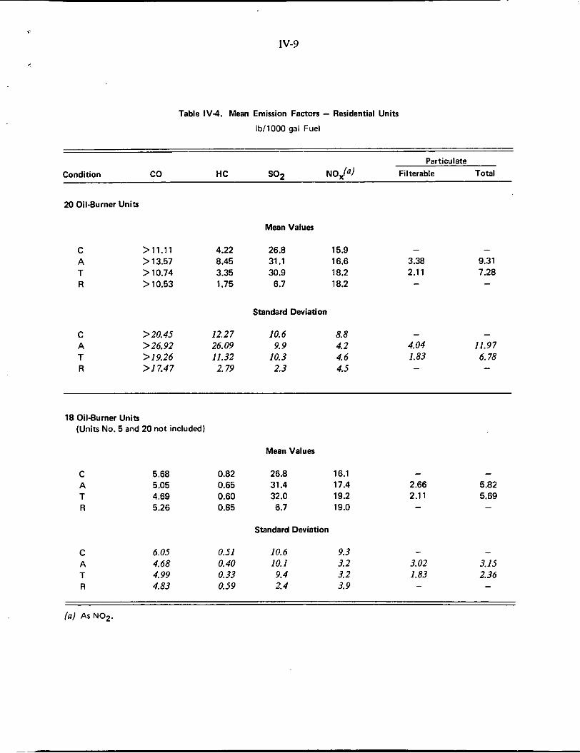
IV-9

Table IV-4. Mean Emission Factors - Residential Units

lbI1000 gal Fuel

Particulate Condition co HC so2 N O P ) Filterable Total

20 Oil-Burner Units

Mean Values

C >11.11 4.22 26.8 15.9 A > 13.57 8.45 31.1 16.6 T > 10.74 3.35 30.9 18.2 R > 10.53 1.75 6.7 18.2

- 3.38 2.11

- 9.31 7.28

Standard Deviation

- - C >20.45 12.27 10.6 8.8 A >26.92 26.09 9.9 4.2 4.04 11.97 T >19.26 11.32 10.3 4.6 1.83 6.78 R >17.47 2.79 2.3 4.5 - -

18 Oil-Burner Units (Units No. 5 and 20 not included)

C 5.68 A 5.05 T 4.69 R 5.26

C 6.05 A 4.68 T 4.99 R 4.83

0.82 0.65 0.60 0.85

0.51 0.40 0.33 0.59

Mean Values

26.8 16.1 31.4 17.4 32.0 19.2 6.7 19.0

Standard Deviation

10.6 9.3 10.1 3.2 9.4 3.2 2.4 3.9

- 2.66 2.1 1 -

- 3.02 1.83 -

- 5.82 5.69 -

- 3.15 2.36 -

f a ) As NO2.

IV-IO

The average particulate emission factors for the tuned and as-found conditions are essentially identical, indicating no effect of tuning on average particulate emission, even though smoke numbers are generally reduced in the tuning operation and particulate emissions from individual units changed considerably upon tuning. The average filterable particulate values for the tuned condition were about 20 percent less than for the as-found condition. This small change would suggest that tuning did not change the nature of the particulates produced.

Except for the HC and SO2 emission factors, the reference fuel data also compare well with data from house fuels. It is to be expected that the SO2 factors would be lower for the reference fuel since the sulfur content of the hydrotreated reference fuel was only. 0.05 weight percent, compared with the average house-fuel sulfur content of the order of 0.2 percent.

The average emission factor for HC using reference fuel was approximately 50 percent higher than that using the house fuels. The higher HC emission factor for the reference fuel is more difficult to rationalize. It is probably not significant, however, since HC emissions are so near ambient levels. It might logically be expected that a higher CO factor would accompany the higher HC factor; this was not observed.

A more extensive discussion of the effect of various burner and tuning aspects and combustion parameters on emission factors is contained in the following chapter.

Gas-Fired Units

Table IV-5 gives the emission factors for the runs on the two gas-fired residential units (in lb/106 cu ft of natural gas), plus the mean factor for aU runs. Also shown are the emission factors for gas-fired residential heating equipment reported in EPA publications(l 12) and equivalent emission factors for oil-fired units. (The values in Table IV-5 can be reduced to emission factors equivalent to lb/1000 gal fuel oil by multiplying by 0.133 to compare the data with results from the oil-fired units.)

The emission factors found in this investigation for the gas-fired residential units are equal to the EPA values for CO, lower than the EPA values for HC and filterable particulate, and higher than the EPA values for NO,. Both sources report negligible S02.

The CO, NO,, and particulate emission factors measured for the two gas-fired units were much less than the mean of the as-found oil-fired units; the HC emission .factors were slightly less than for the oil-fired units.


IV-11

Table IV.5. Emission Factors for Two Gas-Fired Residential Units, Including Comparison With EPA Factors and Mean Factors for Oil-Fired Units

ib/106 cu ft natural-gas input or ib/109 8tu

21 Cold start 27.1 3.6 0 75.6 - - As found 23.4 3.3 0 &.e 4.8 15.4

Tuned 14.6 2.8 0 78.8 - -

22 As found 14.9 6.2 0 89.0 - -

Mean 20.0 4.0 0 81.8 4.8 15.4

-.

EPA.l963(l) 9.4 Neg. 0.4 116.0 19.0 -

EPA-1971 (2) 20.0 8.0 0.6 50.0 19.0 -

Mean for 18 oil-fired units 37.9 4.9 236 131.0 19.9 43.7 in as-found condition

(a) NO, as NO2.

v- 1

d

V. DISCUSSION OF FINDINGS - RESIDENTIAL UNITS

Aside from the numerical emission data, the two most significant points uncovered in this investigdtion of residential units are:

I . Tuning appears to have little effect on reducing emissions from normally maintained units.

2. Steady-state smoke readings do not appear to be good indicators of particulate emissions integrated over several cycles, including start-up and shutdown.

Both of these points have significant implications in view of possible control strategies based on a smoke limit, for example, requiring residential oil burners to be tuned to No. 3 or even No. 2 smoke.

TUNING EFFECTS

In essence, servicemen’s tuning procedures are designed around smoke and C 0 2 readings. Thus, i t might be expected that tuning would reduce HC, CO, particulate, and smoke emissions - with the probable undesirable result that NO, emissions might increase. In fact, however, this was not’always so.

Table V-I is a qualitative compilation, based on emission-factor data, of the effect of tuning on emissions. In a number of situations, tuning did not result in the “expected” change. The plus and minus signs in Table V-1 indicate where emissions of. the indicated pollutant increased or decreased by five percent or more, respectively. The tabulation shows that:

1. HC, CO, and filterable, and total particulate did not always change in the same direction, and

2. In some instances, NOx and combustibles (CO, HC and/or particulate) both increased after tuning.

These results suggest that tuning can result in a variety of effects on the residential units. The effects of tuning may also be examined in terms of the mean emission factors. Table V-2 presents mean emission factors for CO, HC, S02 , NO,, and filterable and total particulate for residential units in the as-found condition for all 20 units and in the as-found and tuned conditions for all units except Units 5 and 20. Identifying and eliminating units in need of replacement (such as Units 5 and 20) accomplishes much more in the way of reducing emissions than f6rther tuning of the other units. It is noted that, for units not needing replacement, tuning had no marked effect on the mean emissions of any pollutant. On the average, tuning resulted in a slight reduction in CO and HC emissions, about a 20 percent reduction in filterable particulate emissions, and an increase in NOx emissions of about 10 perccnt.


v-2

Table V- I . Qualitative Summary of Tuning Effects on Emissions From Residential Units

Change in Pollutant Emission Factor(a) Smoke Number Particulate

Unit &Found Tuned co HC NO, Filterable Total

1 (a) 3.0

2 3.0 3.0 .!= - - - 3/bJ 1 .o 4 7.0 2 .o + + + + 5 (b) oily

7 (b) 3.0 2.0

8 3.5 1 .o - - + + + 9 6.5 1 .o - + +

10 2.0 1 .o - + + + + 11 6.5 3.0 + + + + - 12 3.0 1 .o + - + - - 13 6.0 3.0

14 8.0 2.0 - + + - - - - + - 15 6.0 1.5 +

16 2.0 1.5

17 6.0 0.5

18 4.0 1 .o 20 oily oily

(a) {b)

-

- - + - - -

+and - indicate an increase or decrease exceeding 5 percent. Tuned condition not significantly different than as-found condition; pollutant emissions not recorded.

v-3

Figures V-1 and V-2 show the effect of tuning the burner (to lower smoke numbers) on filterable and total particulate emissions for the individual units. The data from this investigation show that tuning a burner to a lower smoke number was about as likely to increase particulate emissions (either filterable or total) as to decrease them.

Figure V-3 shows the effect on NOx emissions of tuning the individual burners to lower smoke levels. For most units (IO of the 13 units for which smoke number was improved by tuning), tuning the burner to reduce smoke number resulted in an increase in NOx emissions. Although this would likely be attributed to increased flame temperature due to improved mixing, it should be noted that tuning frequently resulted in increasing the excess air and, thus, might have been expected to decrease flame temperature and NOx emissions. However, a portion of the NOx may have been formed as a result of localized “abnormal” conditions, rather than at the average combustion chamber condition.

Follow-Up Measurements

A general question in any such investigation relates to the effect of time on the condition of the space-heating unit. Besides the question of normal day-to-day variability, there is also the question of the effect of time since cleanup (or tuning) on the condition of the burner. To obtain some information on this effect, follow-up measurements were made on two units which had been tuned during the first visit.

Table V-3 presents gaseous emission data and smoke data for the initial and follow-up measurements on two units. In the case of Unit 3, the emission data for the fust and second calls did not show any significant changes. Unit 12, on the other hand, did show some change. In the 6-week interval, the smoke, CO, and HC appear to have increased, although the HC levels (and the CO for Unit 3) were likely below the ambient levels. The lower NO, on the follow-up measurement is consistent with this trend.

These follow-up data are very limited. A more complete examination of follow-up measurements is needed to evaluate the importance of tuneup procedures in reducing emissions. (Some additional follow-up information will be obtained in the Phase I1 investigation.)

PARTICULATE EMISSIONS AN0 SMOKE

Although some data in the Literature show a correlation of particulate emissions with smoke number for a single unit at steady-state condition(l4), data from this investigation indicate that steady-state smoke number was not a direct measure of particulate emissions integrated over several cycles. An earlier study(3) showed similar lack of correlation.

In the present investigation, plots of filterable and total particulate emissions prove to be essentially independent of smoke number (Figures V-4 and V-5). This observation would be expected if the startup and shutdown “puffs” contribute disproportionate quantities of particulate to the integrated value, a not unlikely possibility. Examination of smoke data for the I-, 5-, and 9-minute points did not yield any better correlations.

(14) Hunt, R. A., Jr., and Biller, R. E., Conference Paper CP61-6, Proceedings: API Research Conference on Combustion, API Publication No. 1541 (1961).

B A T T E L L E - C O L U M e U S

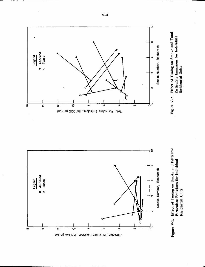
e o

e o

- w

- w

--P

--N

- 0) a c

Legend

VI 0 1

In c 0 In In

.-

.- E w

v-5

30t As-found 0 Tuned

'I 5

0 1 0 2 4 6 0

Smoke Number, 'Bachorach

Figure V-3. Effect of Tuning on NO, Emissions for Individual Residential Units

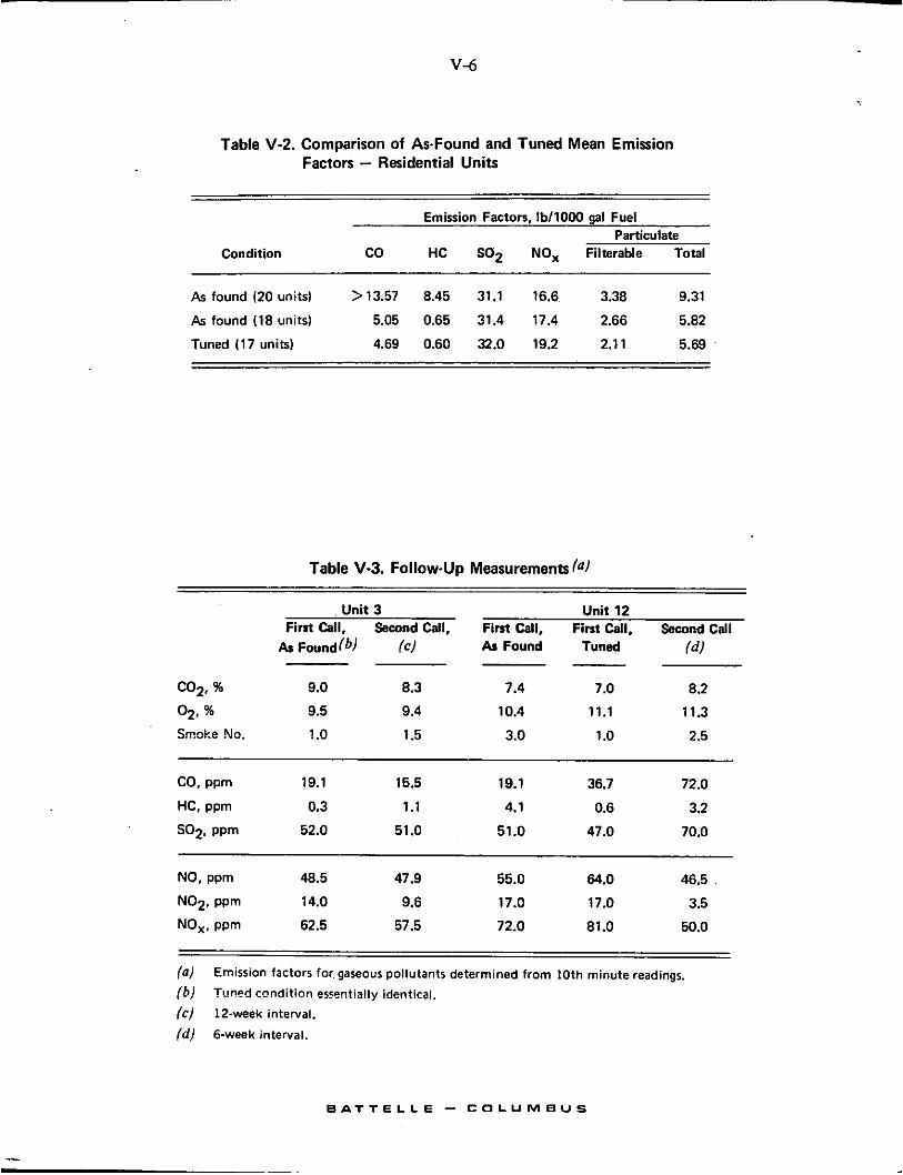
V-6

Table V-2. Comparison of As-Found and Tuned Mean Emission Factors - Residential Units

~ ~

Emission Factors, IbllOOO gal Fuel Particulate

Condition co HC SO2 NO, Filterable Total

As found (20 units) >13.57 8.45 31.1 16.6 3.38 9.31

As found (18 units) 5.05 0.65 31.4 17.4 2.66 5.82

Tuned (17 units) 4.69 0.60 32.0 19.2 2.1 1 5.69

Table V-3. Follow-Up Measurements (a)

Unit 3 Unit 12 First Call, Second Call, First Call, First Call, Second Call

As Found(b) As Found Tuned (d )

co2. % 9.0 8.3 7.4 7.0 8.2

02. % 9.5 9.4 10.4 11.1 11.3

Smoke No. 1 .o 1.5 3.0 1 .o 2.5 ~ ~~

CO. ppm 19.1 15.5 19.1 36.7 72.0

HC. ppm 0.3 1.1 4.1 0.6 3.2

SO2. ppm 52.0 51 .O 51.0 47.0 70.0

NO. ppm 48.5 47.9 55.0 64.0 46.5

N02. ppm 14.0 9.6 17.0 17.0 3.5

NO,. ppm 62.5 57.5 72.0 81.0 50.0

(0)

(b,! Tuned condition essentially identical. (c) 12-week interval.

( d ) 6-week interval.

Emission factors for. gaseous pollutants determined from 10th minute readings.


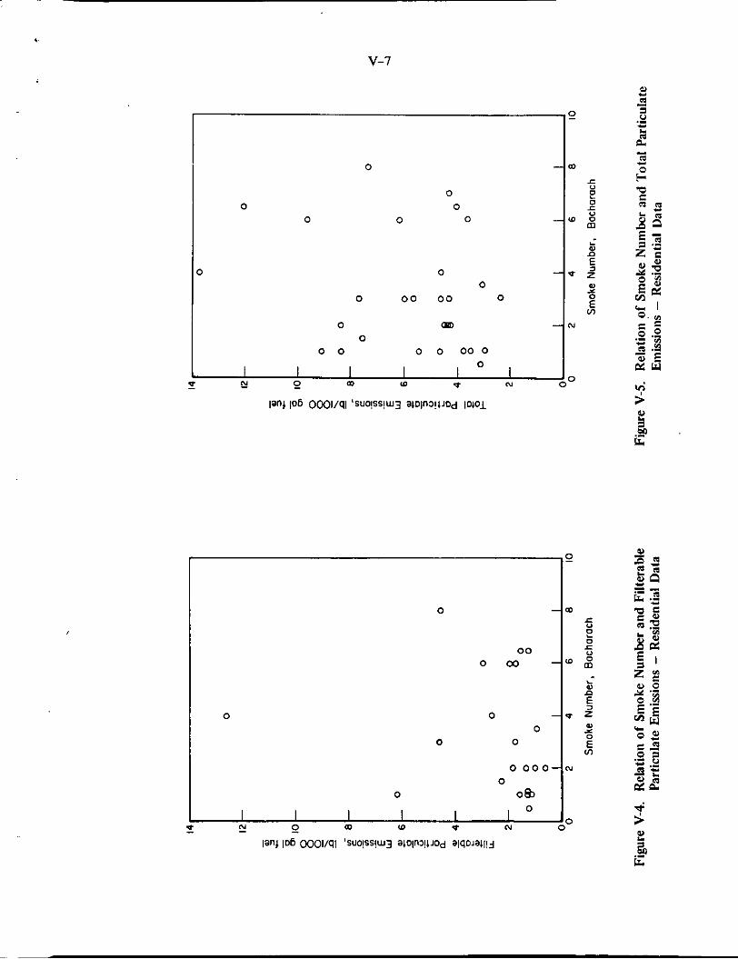
v-7

0

0 0 0

0

00 0

m

0

0 00 0

0

0

00 o m

0 0

0 0

5

4

3

2

I

0

IOC

8C

6C

40

2c

0

V-8

CARBON PARTICULATE EMISSION FACTOR

PERCENT CARBON I N FILTER CATCH / -

-

I I 1 I 2 4 6 8

Smoke Number, Bacharach

Figure V-6. Relation of Carbon Content of Filter Catch and Smoke Number - Residential Units

v-9

As a result of these observations, it can be concluded that steady-state smoke number does not appear to be a suitable basis for standards aimed at limiting the weight of particulate emissions from oil-ftred heating units per unit of fuel input. However, it should be recognized that high smoke numbers, above No. 3 or 4, are indications of tendency for soot buildup on heat exchanger surfaces and, over the long term, this buildup can cause reductions in overall thermal efficiency of the system and can accelerate deterioration of combustion conditions.

Another consideration is that smoke number readings place a greater emphasis on small or low-density particles, which may not contribute significantly to particulate emissions on a weight basis. These particulates are likely to remain airborne longer and be of respirable size. Therefore, smoke number may be a better measure of the health hazard and visibility reduction caused by combustion equipment than is weight of particulate emissions. Additional information in needed on particle size distribution before this aspect can be fully evaluated.

Figure V-6 shows that the carbon content of the filter catch did correlate with smoke number for the limited data available and also shows the relationship of carbon particulate emissions (based on filter catch only) to smoke number. The significance of these correlations is not established, and they should be tested on additional units.

COMPARISON OF RESIDENTIAL BURNER A N 0 UNIT TYPES

It can be useful to examine the data to compare general types of residential burners and installations. The following comparisons were made for smoke number, NO,, and particulate by considering unit types as follows:

Furnaces vs boilers

For high-pressure burners, flame-retention heads and Shell heads vs conventional combustion heads

Matched units vs conversion installations.

Table V-4 shows these comparisons, and some observations are noted below based on average data. These observations should not be considered as f m and significant conclusions, because of the scatter of data, other variables involved, and the fact that the sample size is too small in each case to be representative of an entire class of equipment.

Smoke

From the standpoint of smoke level after tuning, or with reference runs, matched units showed slight advantages, probably due to better mixing. The special and conventional combustion heads were not significantly different in smoke level. Boilers had slightly lower smoke levels than furnaces, an observation that appears t o have no explanation and is possibly a coincidence in the sample of equipment.


v-10

Furnace Boiler

Table V-4. Comparison of Residential Unit Types

Flame retention Conventional + Shell heads heads Comparison

20.0 18.9 3 13

Smoke Number at Tun& Condition

Mean

No. of Units

18.2 20.6 6 9

Smoke Number for Reference Fuel Run

Mean

No. of Units

Filterable Paniculate Emission Factor for Tuned Condition, lb/1000 gal fuel

Mean

No. o f Units

NO, Emission Factor for Reference Fuel Run. ibilOW gal fue,

Mean

No. of Units

1.8 1.5 4 12

1.7 1.6 6 10

I

1.23 1.91 1 8

1.26 2.18 4 5

Matched Conversion

1.5 1.9 1 1 5

1.1 1.2 10 5

1.37 3.61 7 2

18.9 19.9 12 4

v-11

Filterable Particulates

The number of units for which particulate data is available is so limited that comparisons are risky. However, the special burner heads and matched units as categories showed slight advantages in lower particulate for the tuned condition, possibly due to the burner mixing aspect. The particulate-emission mean was lower for furnaces than for boilers, possibly attributable to higher combustion temperatures for furnaces.

NO,

For the reference-fuel runs, furnaces had a slightly higher NO, emission factor compared with boilers - possibly attributable to the fact that the combustion chamber and flame in boilers may operate at lower temperatures, as they generally “see” cooler surfaces. Special combustion heads showed an NO, emission slightly lower than that of conventional heads, possibly due to the greater uniformity of fuel-air mixing (characteristic of newer heads). Matched units had a slightly lower emission factor than conversion installations.

OTHER OBSERVATIONS

Attempts were made to correlate other emission-factor data with various furnace operating parameters. In many cases, no correlation was obtained. However, the lack of correlation may also prove to be of significance and some of these points are noted here.

NO, and Fuel Nitrogen

Unlike the commercial units, where a variety of fuels was used and the nitrogen and sulfur content of the fuel varied, distillate fuels used in the residential units were all low in nitrogen, about 0.05 weight percent. It is not surprising then to observe no correlation of NO, emission factors with distillate fuel-nitrogen content. Likewise, plots of NO, emission factors against firing rates or against C02 show no correlation.

SO2 Measured and Calculated

SO2 levels for the residential units were low as expected in view of the low sulfur content of distillate fuels compared to residual fuels. The question is often raised as to whether SO2 can be satisfactorily calculated rather than measured. I t is a generally well-accepted fact that the sulfur in the fuel oil will be oxidized to sulfur dioxide and, thus, calculating SO2 from a sulfur analysis of the fuel might be sufficient.

Figure V-7 compares measured and calculated SO2 data for the 20 residential oil-burner units. There is some scatter in the data and the measured SO2 values tend to be low. However, at these low levels, SO2 concentration and fuel sulfur determinations are difficult to accomplish accurately. For instance, an error of only 0.05 percent in the sulfur analysis of the fuel produces an error of approximately 4.0 lb/1000 gal in the calculated SO2 value.


v-12

60

- 0) 5 0 - a L - 0 0 0 5 40-

e b Theoretical based on

sulfur content of fuel

\

- c

30 - 0

2 c 0 In In .- .- E

20-

-Range for reference fuel

Calculated SO, Emission Factor, lb/1000 gal fuel

Figure V-7. Measured and Calculated SO2 Emission Factors - Residential Units

0

HC Emission Levels

The data substantiate an important point, namely that the HC levels are too low to be significant. I t should be recalled that in an earlier section it was pointed out that the HC levels being emitted are frequently below, or very close to, ambient levels. (See data in Appendix D, Table D-3.) Thus, with respect to HC, the residential units can “clean up” the intake air.


VI- 1

VI. EMISSIONS FROM COMMERCIAL BOILERS

Eight commercial boilers, as described earlier, were examined in this study. The boilers were operated at 80 percent load, H; an intermediate load, M; - low fire setting, - L; and typical load for the plant, T.

- -

EMISSION MEASUREMENTS

Gaseous-Emission Data

The gaseous-mission data obtained are summarized in Table VI-I. The principal observation in examining these data is the higher levels of SO2 and NO, which are emitted by boilers firing the heavier fuel grades (Nos. 4, 5 , and 6) which contain higher concentrations of sulfur and nitrogen. However, the NO, levels are not solely a function of nitrogen control of the fuel, as f i a t ion may contribute a significant portion of the NO, at higher combustion intensities. The NO, levels increased with increasing load, primarily as a result of the higher intensity combustion.

CO and HC emissions are low and, in fact, are not significantly higher than emissions of residential units (or observed background levels).

The linkage controlling fuel/air ratio a t different levels lacked proportionality for some boilers at low loads. Higher excess air at low loads resulted in lower ppm levels of S02.

For purposes of evaluating the experimental techniques and the data, a comparison can be made’between calculated C02 and SO2 values (with excess air based on oxygen content of the flue gas) and measured values of C02 and S02. Table VI-2 compares calculated and measured values for C02 and SO2 and for NO,, assuming that all of the C, S, and N in the fuel appear as C02, S02, and NO, in the flue gas. The assumption is sufficiently sound for C 0 2 and S02; however, the NO, calculations should be considered only on hypothetical grounds. The calculation assumes that all the nitrogen in the fuel appears as NO,, and ignores NO, formed by fixation of nitrogen in tFe air. This is not, in fact, the case; only a portion of the NO, is attributed to chemically bound fuel nitrogen, the remainder of the NO, being the result of nitrogen fixation.(l5,16,17)

The C02 measurements agree well with the calculated C02. In the instance where the agreement was not good (C1007, Run M), it appears that the 0 2 measurement may have been in error.

(15) Paterson, R. E., “Nitrogen Oxides in Combustion Gases”, Internal Report, Chevron Research Corporation, File 084.0, April I I , 1961.

(16) Martin, G. B., Pershing, D. W., and Berkau, E. E., “Kinetics of the Conversion of Various Fuel Nitrogen Compounds to Nitrogen Oxides in Oil Fired Furnaces”, AIChE Paper No. 37f, 70th National Meeting, Atlantic City, August 29-September I , 1971.

(17) Bartok, W . , Engleman, V. S., Goldstein, R., and Vane, E. D., “Basic Kinetic Studies and Modeling of Nitric Oxide Formation in Combustion Processes”, AIChE Paper 37d, 7 0 National Meeting, Atlantic City, August 29-September I , 1971.

B A T T E L L E - C O L U M e U S

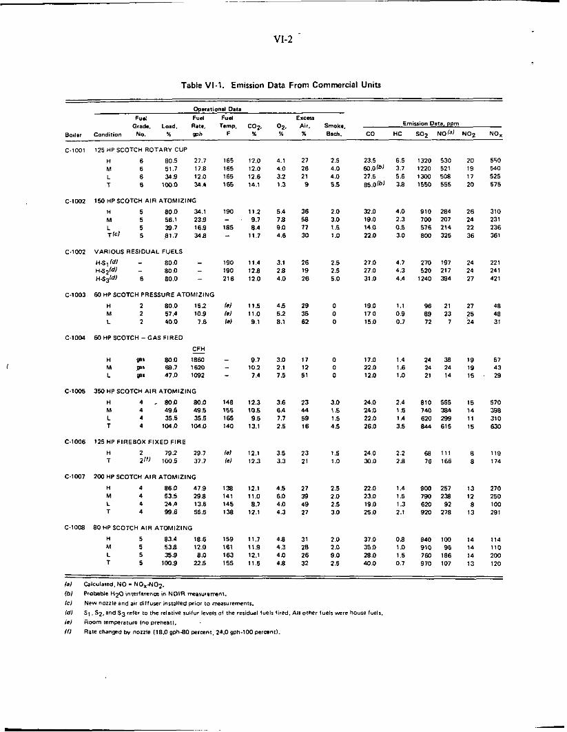
VI-2

Table VI.1. Emission Data From Commercial Units

0p.r.tion.l 0.1.

FUh. Fual Fuel E I C s u Grad.. Load. Rata. Temp, CO2. 02, Air, Smoke, Emission Data, ppm

EO HC SO2 Nola) NO2 NO. 0ail.r Condition No. b wh F 4 X 4 0ach.

C.1001 125 HP SCOTCH ROTARY CUP

H 6 80.5 21.1 165 12.0 4.1 21 2.5 23.5

L 6 34.9 12.0 165 12.6 3.2 21 4.0 21.5 T 6 1W.O 39.4 165 14.1 1.3 9 5 5 85.0fb)

M 6 51.1 17.8 165 12.0 4.0 26 4.0 60.o1bl

C-lW2 150 HPSCOTCH AIR ATOMlZlNG

H 5 80.0 34.1 190 11.2 5.4 36 2 .o 32.0 M 5 56.1 239 - . 9.7 7 8 58 3.0 19.0 L 5 39.7 169 185 8.4 9.0 17 1.5 14.0 TIC) 5 81.1 348 - 11.7 4.6 30 1 .o 22.0

n.s1 Id1 - 60.0 - 190 11.4 3.1 26 2.5 21.0

C.1002 VARIOUS RESIDUAL FUELS

H S ~ l d l - 80.0 - I90 128 2 8 19 2.5 27.0 H.s31dl 6 80.0 - 216 12.0 4.0 26 5.0 31 .O

c.1003 m HP SCOTCH PRESSURE ATOMIZING

H 2 80.0 152 Id 11.5 4.5 29 0 19.0 M 2 51.4 10.9 kl 11 D 5.2 35 0 110 L 2 40.0 1.6 IS) 9.1 8.1 62 0 15.0

C.IOM m HP SCOTCH - G A S FIRED

E H sr 80.0 ma M P* 69.1 1620 L ss 41.0 1092

c . 1 ~ 350 w SCOTCH AIR ATOMIZING

H 4 . 80.0 80.0 M 4 49.6 49.5 L 4 35.5 3 5 5 T 4 104.0 104.0

C.1006 125 HP FIREBOX FIXED FIRE

H 2 19.2 29.1 T 21') lW.5 31.1

- 9.1 3.0 1 1 0 11.0 - 10.2 2.1 12 0 22.0 - 1.4 7.5 51 0 12.0

148 12.3 3.6 23 3.0 24.0 155 105 6.4 44 I 6 14.0 165 9.5 7.7 59 1.5 22.0 140 13.1 2.5 16 4.5 26.0

Id 12.1 3.5 23 1.5 24.0 Id 12.3 3.3 21 1 .o 30.0

C.lW7 2p0 HP SCOTCH AIR ATOMIZING

H 4 86.0 41.9 138 12.1 4.5 2 1 2.5 22.0 M 4 53.5 298 141 11.0 6.0 39 2 .o 23.0 L 4 24.4 13.6 145 8.7 4.0 49 2.5 19.0 T 4 99.6 55.5 138 12.1 4.3 21 3.0 25.0

C-I008 80 HP SCOTCH AIR ATOMIZING

H 5 83.4 18.6 159 11.1 4 8 31 2 .o 31.0 M 5 5 3 8 12.0 161 11.9 4.3 28 2 a 35.0 L 5 359 8.0 163 12.1 4.0 26 9.0 28 .O T 5 1009 22.5 155 11.5 4 8 32 2 .5 40.0

6.5 1320 530 20 3.1 1220 521 19 5 .6 1303 508 17 3 8 1550 555 20

4.0 910 264 26 2.3 700 201 24 0.5 516 214 22 3.0 800 325 36

4.1 210 191 24 4.3 520 211 24 4.4 1240 394 21

1.1 96 21 21 0.9 89 23 25 0.1 12 7 24

1.4 24 38 19 1.6 24 24 19 1.0 21 14 15

2.4 810 555 15 1.6 140 384 14 1.4 620 299 11 3.5 844 615 15

2.2 6 8 1 1 1 8 2.8 16 166 6

1.4 9W 251 13 1.5 190 238 12

2.1 9x) 278 I3 1.3 6m 92 8

0 8 940 1W 14 I D 910 96 14

0.1 910 101 13 1.5 i m 186 14

550 540 525 515

310 231 236 361

221 241 421

48 48 31

57 43 29

510 398 310 630

119 114

210 250 IO0 29 I

I14 110 2W 120

- -

VI-3

Table V I 2 Calculated and Measured Flue Gas Composition, Based on 0 2 Measurement and Fuel Properties - Commercial Boilers

coz. % SOz. ppm NO,. ppm 02. Boiler Condition % Calc'd Meas'd Calc'd Maas'd Cals'd(0) Mem'd

ClOOl

c 1002

c1002

C1003

ClOM

ClOffi

C 1006

C1007

ClOCs

H M L T

H M L T

H .S 1

H.S3

H M L

H M L

H M L T

H T

H M L T

H M L T

H 52

4.1 4.0 3.2 1.3

5.4 7.8 9.0 4.6

3.1 2.8 4.0

4.5 5.2 8.1

3.0 2.1 7.5

3.6 6.4 7.7 2.5

3.5 3.3

4.5 6.0 4.0 4.3

4.8 4.3 4.0 4.8

12.1 12.2 12.8 14.3

11.1 9.3 8.3 11.7

12.6 13.0 12.2

11.5 11.0 8.8

- - -

12.4 10.3 9.3 13.2

12.2 12.4

11.7 10.6 12.1 11.9

11.6 11.9 12.2 11.6

12.0 1190 12.0 1190 12.6 1250 14.1 1390

11.2 761 9.7 636 8.4 575 11.7 8 W

11.4 286 12.8 542 12.0 1250

11.5 99 11.0 94 9.1 76

9.7 - 10.2 - 7.4 -

12.3 954 10.5 791 9.5 715 13.1 1020

12.1 131 12.3 133

12.1 901 11.0 815 8.7 930 12.1 913

11.7 926 11.9 957 12.1 975 11.5 926

1320 1220 13W 1550

910 700 576 8 W

270 520 1240

96 89 72

24 24 21

810 740 620 844

ea 76

900 790 620 920

940 910 760 970

515 520 545 607

354 297 267 375

197 316 460

30 29 23

- - -

265 220 199 282

28 28

25 1 226 259 254

235 243 247 235

550 540 525 575

310 2 30 236 360

220 240 420

48 48 30

57 43 29

570 398 310 630

118 174

270 250 100 290

114 110 200 120

/ a ) Calculated assuming 100% Converlion of fuel nitrogen and no nitrogen fixation. Sea text. p VI.]

v1-4

Examination of the SO2 data suggests that the SO2 measurements for Units ClOOl and ~ 1 0 0 2 were slightly high. Some trouble was experienced in the field measurements at the point when the field team shifted from residential to commercial measurements. The heavier particulate loading and higher sulfur level of the commercial units required that the monitoring equipment be cleaned more frequently and that the gas stream be filtered more efficiently.

Although the assumptions made in calculating NOx are based on rather hypothetical grounds, i t is interesting to note that a general correlation exists between nitrogen content of the fuel and measured NO,. Figure VI-l shows the correlation for the fuel oils and units examined. (Boiler C1005 is the only unit for which data did not correlate reasonably well.) The correlation is particularly strong where four fuels of different nitrogen content were fired in Boiler C1002. However, fuel properties other than fuel nitrogen (e& viscosity, gravity, etc.) vaned for the four fuels fired in this boiler, and the quantitative influence of these properties on the correlation between NOx and nitrogen in the fuel is unknown. .

Particulate Loading

Particulate loadings for the commercial boilers, both measured and corrected to 12 percent C02, are tabulated in Table VI-3. Examination of the smoke and particulate loading data suggests no direct relationship between the two parameters. Likewise, particulate loading and fuel grade show no positive correlation. The highest loading was observed in Unit C1002, Run H43, where a No. 6 fuel oil was fired with insufficient preheat. Although not evident in all runs, in most the particulate loading was higher at 80 percent load than at reduced loads.

EMISSION FACTORS

Oil-Fired Boilers

Emission factors for the gaseous species and particulates for the oil-fired commercial units are presented in Table VI-4. The data are presented as lb/1000 gal fuel. Appendix G includes convcrsiori factors for obtaining emission factors in other units, such as lb/1000 Ib fuel, Ib/million Btu fuel input, and Ib/million standard cubic feet of flue gas at 12 percent C 0 2 (the last for particulates only).

Table VI-5 shows mean values and standard deviations for the emission factors for the commercial boilers. These values are presented separately for distillate and residual fuel oils and for all fuel oils. They are also presented separately for all runs at 80 percent load (Condition H) and for all loads.

As is the case of the residential units, the CO and HC factors are fairly low. The mean values for the SO2 factors are significantly higher than those obtained in the residential units. This obviously is related to the higher sulfur content of the fuels used in the commercial units. A word of caution in examining the SO2 emission factors is in order; the mean average value may be misleading since it averages all the commercial fuels used, which ranged from 0.2 to 2.4 weight percent sulfur.

Table VI-6 presents SO2 emission factors in lb/1000 gal per % S. These factors are more useful for interpreting SO2 emissions. The mean emission factor on this basis is 145.


E a a

d z

VI-5

Legend

Boiler C1002 with four fuels 0 Other boilers

0 0

7 /

/

0 0

0. I 0.2 0.3 0.4

Nitrogen in Fuel, weight percent

0.5

Figure VI-1. Relation of Measured NO, and Fuel Nitrogen

(Commercial boilers at 80 percent load and fuel-nitrogen content from Table B-3)

VI-6

(DN !=g 0 0 0 0

+ C D

m u z g P O N P O m m n N

VI-I

Table VI4. Emission Factors - Oil-Fired Commercial Units

lb/1000 gal fuel

Fuel Grade, Particulate

NO,/") Filterable Total Unit Condition NO. co HC s o 2

C l O O l H M L T

c 1002 H M L T

c1002 H.S1

H.S3 H.S2

c1003 H M L

C1006

C1007

C1005 H M L T

c 1008 H M L T

- - 6

2 2 2

4 4 4 4

2 2

4 4 4 4

5 5 5 5

3.19 0.50 8.13 0.29 3.56 0.41 9.94 0.25

4.53 0.32 3.12 0.22 2.58 0.05 2.98 0.23

3.51 0.35 3.37 0.31 4.16 0.34

2.41 0.08 2.21 0.07 2.36 0.06

3.07 0.18 3.60 0.14 3.62 0.13 3.13 0.24

2.89 0.15 3.57 0.19

2.91 0.11 3.33 0.12 2.95 0.12 3.28 0.16

5.04 0.06 4.67 0.08 3.67 0.1 1 5.50 0.06

410. 378. 385. 415.

294. 263. 243. 248.

80. 148. 381.

'28. 26. 26.

237. 254. 234. 233.

19. 21.

272. 262. 220. 277.

293. 278. 228. 305.

115. 113. 105. 104.

68. 59. 68. 76.

44. 46. 87.

10. 7.

11.

112. 92. 79.

117.

22. 32.

55. 56. 24. 59.

24. 23. 41. 26.

20.9 31.3

12.1 26.3

- -

11.6 37.9

8.6 44.3 - -

- -

12.0 47.8 8.4 17.7

40.0 76.0

1.5 18.2

4.4 10.7

9.0 35.7

7.7 16.9

- -

- -

2.3 12.2 - - 7.9 21.1

7.5 14.8 - -

- - 8.8 18.0

17.3 32.5 - -

- -

fa] NOx as N02.

VI-8

Table VI-5. Mean Emission Factors - Oil-Fired Commercial Boilers lb/1000 gal fuel

Particulate

Fuel Condition co HC SO2 NO,(a) Filterable Total

Distillate (No. 21

Mean Values

H 2.65 0.12 24. 16. 1.9 15.2 All 2.69 0.1 1 24. 16. 2.7 13.7

Residual H(b) 3.75 0.23 301. 75. 11.6 28.8 (No. 4, 5, and 6) All(c) 4.08 0.21 276. 69. 13.2 32.3

All fuel oils H 3.59 0.24 222. 58. 8.9 24.9 All 3.83 0.19 230. 60. 11.3 28.8

Standard Deviation

Distillate

Residual

H (dl (dl (4 (4 (4 (dl

H(b) 0.97 0.18 65. 39. 5.4 8.8

All 0.55 0.06 3.8 10.4 1.5 4.0

1.74 0.12 80. 32. 9.0 17.0

All fuel oils H 0.85 0.16 146. 43. 6.5 10.0 All 1.68 0.12 122. 36. 9.1 17.0

(a) NO, as N02.

(b) (c) (d)

Does not include runs on Boiler C1002 with fuels 51. 52, and 53. Includes runs on Boiler C1002 with fuels 51. 52. and 53. Standard deviation meaningless a s only two runs are in this category.

VI-9

Table VI-6. Sulfur Dioxide Emission Factors (on a Percent Sulfur Basis)

% S Emission Factor Boiler Condition in Fuel oer % Sulfurla)

ClOOl H M L T

c1002

c1002

C1003

c1005

c1006

C1007

ClO08

H M L T

H 6 1

H 4 3

H M L

H M L T

H T

H-S2

2.30 178 2.30 164 2.30 167 2.30 180

1.62 181 1.62 162 1 .e2 150 1.62 153

0.53 151 0.98 151 2.43 157

0.20 140 0.20 130 0.20 130

1.81 131 1.81 140 1.81 129 1.81 129

0.25 76 0.25 84

1.81 150 1.81 145 1.81 122 1.81 153

1 .89 162 1 .a9 154 1 .89 126 1 .89 168

Mean 145

Standard Dev. 25

(0) LbI1000 gal fuel per % S.

VI- IO

The NO, emission factors were significantly greater for the commercial boilers than comparable residential emission factors, reflecting the higher fuel-nitrogen content and the higher intensity combustion.

Additional discussion of the significance of these results and their correlation with important variables is contained in Section VIl.

Gas-Fired Boiler

Table VI-7 gives emission factors for the gas-fired runs in Boiler C1004. These data show higher CO and SO2 emissions for this one unit than the currently reported EPA values. The emission factors for HC and filterable particulate are substantially below the EPA values. The high level of SO2 emissions is probably related to deposits in the boiler from earlier oil-fired Nns.

Emission factors for natural-gas firing were about the same as those for oil firing for CO and HC and were substantially below those for oil firing for NO, and particulate. (Multiply emission factors in lb/106 cu ft of natural gas by 0.133 to convert to a Btu value equivalent to 1000 gal of No. 2 fuel oil.)

Table VI-7. Emission Factors for Gas-Fired Commercial Boilers, ib/106 cu ft Natural Gas

Particulate Unit Condition co HC so., NO, Filterable Total

c1004 H 23.8 1.1 77 101 18 36

- - M 21.2 1 .o 85 70

L 29.4 1.2 73 76 4 21

Mean 24.8 1.1 78 82 11 29

E P A - I ~ ~ ~ ) 0.4 Neg. 0.4 116 19 -

€PA-1971 (2) 20 8 0.6 100 19 -

E A T T E L L E - C O L U M ~ U S

VII-I

VII. DISCUSSION OF FINDINGS - COMMERCIAL BOILERS

Within the scope of this investigation on commercial boilers, the principal parameters which showed some pattern of correlation were fuel nitrogen and firing rate as they affected NO, emissions. As shown in Table VI-6 in the previous section, sulfur dioxide emissions are proportional to sulfur content. In addition, fuel type had some influence on smoke and particulate emissions. Smoke and particulate data for the commercial boilers showed poor correlation. These aspects are further discussed in the following section.

FACTORS INFLUENCING NO,

Increasing either fuel nitrogen or firing rate generally tended to increase NO, emissions, although examples contrary to this general trend are evident. Undoubtedly, NO, emissions are related to both of these factors, as well as other parameters.

Fuel-Nitrogen Effect

Figure VII-1 shows measured NO, emission factors (as N 0 2 ) plotted against nitrogen content of the fuel. As pointed out with respect to Figure VI-1 showing NO, ppm levels, there appears to be a general trend for NO, emission factors to be higher for the fuels containing greater quantities of nitrogen. This is particularly true when viewing the data from firing four different fuels in Boiler C1001. However, there is sufficient scatter in the data to suggest that other variables, i.e., nitrogen fmation, also have an important influence on NO, emissions. The fact that some points are well below the curve suggests that the combustion process might be modified to provide low NO, .combustion.

FiringRate Effect

Figure VII-2 presents a plot of NO, emission factors as a function of firing rate. The plot shows that all NO, data were above a lower boundary which increased with fming rate. This is not surprising in that combustion temperature generally increases with firing rate in real systems due to the reduced surface-to-volume ratio of the flame which reduces heat transfer from the flame.

Also shown on Figure VII-2 are the ranges of nitrogen contents of the fuels for different data points. It can be seen that the runs with higher nitrogen content fuels tended to have NO, emission levels farther above the curve of minimum NO,.

FACTORS INFLUENCING SMOKE AND PARTICULATE

It is difficult to separate the many variables which may affect smoke and particulate, but several factors are normally expected to contribute - including atomization, fuel-air mixing, and fuel characteristics. In this investigation, atomization and fuel-air mixing were not examined, except indirectly as fuel viscosity and overall atomizing methods were involved.


VII-2

160

140

120

100

80

60

40

20

-

-

-

-

-

- 0

0 - Q 0

e 0

L e g e n d

Boiler C 1002 at 80% load Other boilers and loods

0 0

0

0 e

8

0 : 0 e

0

0 0

Q

e

01 I I I I 0 0. I 0.2 0.3 0.4 0.5

Nitrogen in Fuel, percent

Figure VII-1. Relation of Fuel Nitrogen and NO, Emissions

(Commercial boiler runs at all loads and firing condirions; Cue1 nitrogen dala from Table B-3)

180

160

140

In c 0 In In .- .- E w 60

0" z

40

20

0

VII-3

Legend

Fuel Nitroqen Content

- +

0 0.023 -0.025 '10 + 0.16 - 0.25 '10

0.33-0.39 O/o

rn

rn

e

0.44 O/o

rn

0

+ e

e

e f

$

Firing Rate, gph

Figure WI-2. Relation of Firing Rate and NO, Emissions

(Commercial boiler runs at all loads and firing conditions, with fuel nitrogen contents identified)

Fuel Viscosity

Figure VII-3 is a plot of smoke and filterable particulate emission factors vs the fuel ‘viscosity estimated for the firing temperature.* With the exception of the data for the rotary burner of Boiler C1001, this shows that, as expected, lower smoke and particulate emissions were generally observed at lower atomizing viscosities, even though both air and pressure atomizers were involved.

Fuel Type

To examine the effect of fuel properties other than viscosity, API gravity was used as a general indicator of fuel composition, the heavier fuels having lower values of API gravity.

Figure VI1-4 shows a plot of smoke vs API gravity for the commercial boilers operating at 80 percent load; this reveals a general trend toward lower smoke for fuels with higher API gravities, but with considerable scatter of data. Figure VIId shows similar plots for particulate emission factors; here filterable particulate yielded a somewhat more consistent relation than total particulate.

Fuel-Ash Content

Figure VII-6 shows that there is not a strong correlation between filterable particulate and ash content of the fuel. In fact, fuel ash only accounted for an average of about 25 percent of the filterable particulate emissions.

TRIAL CORRELAT’IONS OF SMOKE VS PARTICULATE

Figures VII-7 and VIE8 illustrate an attempt to investigate the possible correlation of smoke and particulate for the data on commercial boilers; smoke measurements are more convenient and a correlation would be useful for different types of equipment. However, particle-size differences can interfere with the correlation.

Figure VII-7 compares particulate emission factors with smoke number, and Figure VI1-8 compares measured particulate loadings with smoke numbers.

As found in the residential class of equipment, it is apparent that the attempted correlations are too indefinite for smoke to be a reliable indicator of particulate loading emissions for commercial boilers.

‘The atomizing viscosity was estimated from data at 100 F using slopes typical for fuel oils, although the low- sulfur-residual oils S 1 and S2 may possibly have different temperature-viscosity characteristics.


VII-5

30

20

10

I Legend

'

'

0 Boiler C- 1002. air atomizing Other boilers

0 Rotory atomizing A Pressure atomizing

FILTER ABLE PARTICULATE

0 Air atomizing

+O t s3

- 0

A 0 I I A I I I I

"I SMOKE

t

0

I I A I I I I 20 30 50 100 200 300 5

Fuel Viscosity, SSU at atomizing temperature ( log scale)

Figure VII-3. Relation of Firing Viscosity to Smoke and Filterable Particulate for the Commercial Boilers Operating at 80 Percent Load, Condition H -

I I I I n l 20 30

8

c

0 r 0 z - b n E t al 1 0 E v)

Legend

Boiler Cl002, 4 fuels 0 Other boilers

6 - . s3 4-

0

0 s, . 0 SI 2- 0.

0

I API Gravity at 60 F

Figure VU-4. Relation of Fuel Gravity and Smoke Number for the Commercial Boilers Operating at 80 Percent Load, Condition - H

9

VII-7

- Q) a c - 0 0

0 0 Q e \ - L

c 0 0 0 LL c 0 In ln .- .- E

W

0)

0

0

o

c - a .- c L

a

4c 0 F I LTER ABLE PARTICULATE

0 0

0 0 0 0

I I I I 01 0

0 IO 20 30 40

0

0

TOTAL PARTICULATE

0

0 0

0 00 0

0

0 20 30 10

API Gravity at 60 F

Figure VIM. Relation of Fuel Gravity and Particulate Emission Factors for the Commercial Boilers Operating at 80 Percent Load, Condition.;

vii-8

44

40

1 24

20

16

12

8

4

0

0

0

0

0 0

0 0 0 0 8

0

0-

10 \’ Contribution of ash to emission factor, calculated 0

0 0

0 1 0-

0 0 0 0 0~

4 1 1 1 0.02 0.04 0.06 0.08 C

Ash in Fuel Oil, percent

Figure VII-6. Contribution of Ash in Fuel Oil to Filterable Particulate Emissions - Commercial Boilers

VI1-9

50

40

- al a c - 0 0

0 0 0 e \

~

L

c 0 0 0

L L

c 0 u) in

.-

.- E

W

a 0

0

c - a .- c L

2

Legend FILTER ABLE

Boiler C1002 PARTICULATE 0 Other Boilers

s3 -

Figure VII-7

SI

0 0

0

. O t 0

s3

TOTAL PARTICULATE

0

0

I I I I

Smoke Number, Bachorach

2 4 6 8 I

'. Trial Correlation of Smoke Number and Particulate Emission Factors - AU Data for Commercial Boilers, Conditions fi and - L

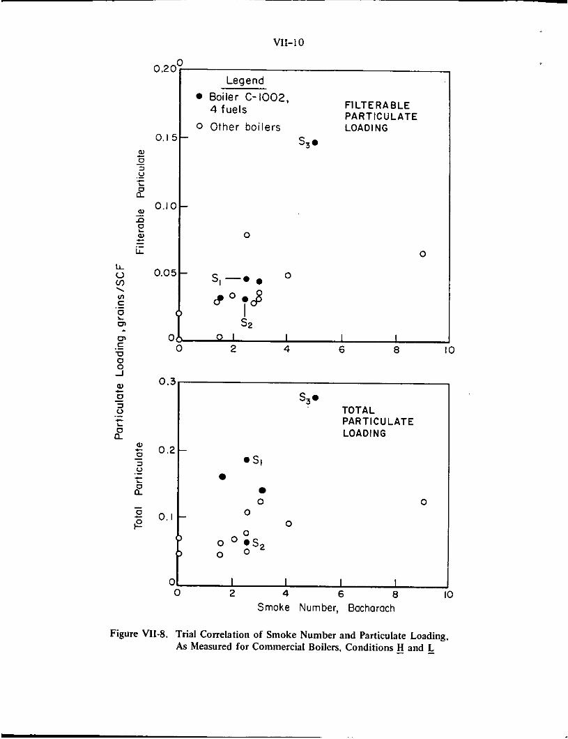
0.2

VII-10

Legend .

0 Boiler C-1002, FI LT E R A B L E P A R T I C U L A T E 4 fuels

0 Other boilers LOADING

S3. 0. I

0

0 s,-* 0 0.051

O b 0 1 I I I 0 2 4 6 8

0.:

0.2

0. I

c

.SI

0 0

T O T A L PAR T I C U L A T E LOADING

S3@

0

0 0

0 0 O S , 0 0

I I I I 2 4 6 8

Smoke Number, Bachorach

Figure VII-8. Trial Correlation of Smoke Number and Particulate Loading, As Measured for Commercial Boilers, Conditions H and L - -

6

VIII-I

VIII. ACKNOWLEDGMENTS

The authors wish to acknowledge the assistance of the API SS-5 Task Force for helpful comments during the course of this program. Membership on the SS-5 Task Force was as follows:

E. Landau (Chairman) . . . . R. C. Amero . . . . . . . . S. P. Cauley . . . . . . . . H. E. Leikkanen . . . . . . . B. L. Mickel . . . . . . . : R. E. Paterson . . . . . . . . C. W. Siegmund . . . . . . . R. A. Beak. . . . . . . . . J. R. Could. . . . . . . . .

Asiatic Petroleum Corp. Gulf Research & Development Co. Mobil Oil Corporation Texaco Inc. American Oil Company Chevron Research Co. Esso Research & Engineering Co. National Oil Fuel Institute, Inc. American Petroleum Institute

In addition, the assistance of the Commercial-Industrial Air-Pollution Committee of the American Boiler Manufacturers Association is acknowledged for their cooperation in the selection of commercial units and assistance in defming appropriate test conditions.

Acknowledgment is made of the assistance of Gulf Oil Corporation in providing the distillate reference fuel, and of Esso Research and Engineering Company for assistance in providing the low-sulfur residual fuels and the analysis of all the commercial fuels.

Special acknowledgment is due the cooperation and patience of the homeowners who permitted the field team to move in and set up the battery of instruments and who tolerated the inconvenience of having normal comfort control of their heating system interrupted during 2 or 3 days of measurements. The authors also wish to acknowledge similar cooperation by the manufacturers of the commercial equipment, plus their providing services of skilled service technicians to assist in adjustment of conditions.

The authors are also indebted to numerous Battelle-Columbus staff members who con- tributed to various aspects of the program. Special acknowledgment is made to Technicians J. J. Fancelli and G. F. Ward who served on the field team making the measurements,* and to various supporting staff to D. R. Hopper and D. W. Joseph for their assistance in the computer analysis of data; to R. E. Heffelfinger, L. J. Hillenbrand, F. E. Huber, and W. E. Schwartz who conducted the analytical measurements for the particulate characterization; and to the patient secretaries who assisted in the tabulation of data and preparation of this report.

'Authors of this report who served on the field team during portions of the investigation are S. E. Miller, E. 1. Schulz, R. H. Melvin, and Consultant W. H. Axtman.


. . . i

. . . . . . . . . . . . . . . . .

. .

..

. . . . . . . . . . .

. . . . .

. - I . .

<. . -. . .. . .

. . A. BACKGROUND DATA ON OIL-BURNER POPULATION

6. FUEL ANALYSES

C. DETAILS OF FIELD PROCEDURES

.D. SAMPLING AND ANALYTICAL PROCEDURES FOR GASEOUS

. > I

. .

. . . . , .

' EMISSIONS

. . . E. SAMPLING AND ANALYTICAL PROCEDURES FOR PARTICULATE AND SMOKE

. . . . . . F. CHARACTERIZATION OF PARTICULATE SAMPLES

. G. DETAILS OF EMISSION-FACTOR CALCULATIONS AND ..... . . . . - . . . .

. . . . .- .

CONVERSION FACTORS ~.

. . . . . . . . . . ... .. . . . . . . . . . . . . . . . . . .

. . H. REFERENCES

%

. . . . . . . . . . . . . . . . . . . . . . . _ .

. . . . . . . ~ - . . .I.'.. ~ . . . . . . . - . . . . ..; . ' . . . . -~ . . . . . . _ . . .

. I , , . . . .

. . , . L . . .

. . . . . . . . . . , . . . . . . . . . . . . . . . . . . . . . . . . , . , . . . - . . . . . . .

. , . I .. . . . . . . . . . . . . . . . . . . . .,-. . . . . . . . . . . . . . . . . . . <:.. . . . . . . . . . ,

._ . . . . . .- . . . . . . . .. - . .

. . . . . .

. .

. . . .

. . . . . . , .

. .

. . . . . . . . . . . . . . . . . . . . . . . - - . - . . . . . . . . . . .... . . . . . . . . . . , . . . . . . . . . . . . . . . . . . ... . . . . . .

. . . ... . . . . . . . . . .

. I

. _ . > . . . . . . .

. . . I . , . .. . . . .

. - .

. . . . . . . . . . . . . . . . . . . . . . " . ' , . . . , , . .

. . . . .

. . . . . . . . - .

. . . . . . . .

. .;..

. . . . . . .

..

. . . . .

. * ; . .

. . . . . . .

. .

. . . . . . . . . .

. . . . . . - .

. . . . . . . . . . . . . ,

' . ' I * . k _ . . . . .

. . . . . . . . . . . .

. . - .

, - . . . . .

. . , . . ' _ . '

. .

. . . . . . . .

. . . .

. .

. . .. . .

. , - B A T T E L L E ' - C 0 L U M S U S , .

. . I

. .

.: A- 1

APPENDIX A

BACKGROUND DATA ON OIL-BURNER POPULATION

Residential Units

Tables A-1 through A-4 provide background data used in the selection of the residential equipment mix included in this investigation. Although a general survey of the existing burner population by detailed burner and system type is not available, data contained in these tables provides a guideline for estimating the population and selecting a representative equipment mix.

Commercial Boilers

Table A-5 provides data on commercial-industrial boiler sales by burner (atomizer type) and by fuel for a recent year. Again, these data serve as a guide in selecting a representative equipment mix.

Table A-1. Oil-Fired Equipment Population (a)

Units in Service Units Sold End of 1970, in 1970,

Equipment Type thousands thousands

Central Heating, Residential Sizes 11,300 472

Oil-Fired Furnaces(b) 5,900 347

Oil-Fired Water Heaters 20Old 49 le)

Commercial-Industrial, >6.0 gph 1,100 39

Oil-Fired Boilers 5,400 139

(a) Source: Fueloil and Oil Heat. (b) Includes mobile-home installations. (e) Estimated.


A-2

~~~ ~

Table A.2. Sales of Domestic Oil Burners by Type (a)

1969, he-1941, Oil Burner Type percent percent

High-pressure Gun Burners 95.0 71.7

Low-Pressure Burners 3.4 6.2

Vertical-Rotary Burners 0.4 11.0

Vaporizing Burners 1.2 10.8

Miscellaneous Types - 0.3

(a) Source: Fueloiland Oil H a t .

Table A-3. Distribution of Sizes of Domestic Oil-Fired Equipment (Data for 1970 Sales) la)

By Firing Rates, gph, All 197G installations

Rat0 Percent

< 1.0 32

1.0- 1.35 37

1.35- 1.65 12

1.66 - 2.0 7

2.01 - 3.0 7

> 3.0 5

-

By Boiler Sizes, 1@ Btuh

Size Percent

< 75 3

76 - 100 26

101 - 125 45

126 - 150 16

> 150 10

-

By Furnace Sizes, 1@ Btuh

Size Percent

< 50 2

50 - 75 11

76 - 100 42

101 - 125 32

> 125 13

-

(a) Source: Fueloiland Oil Heut.

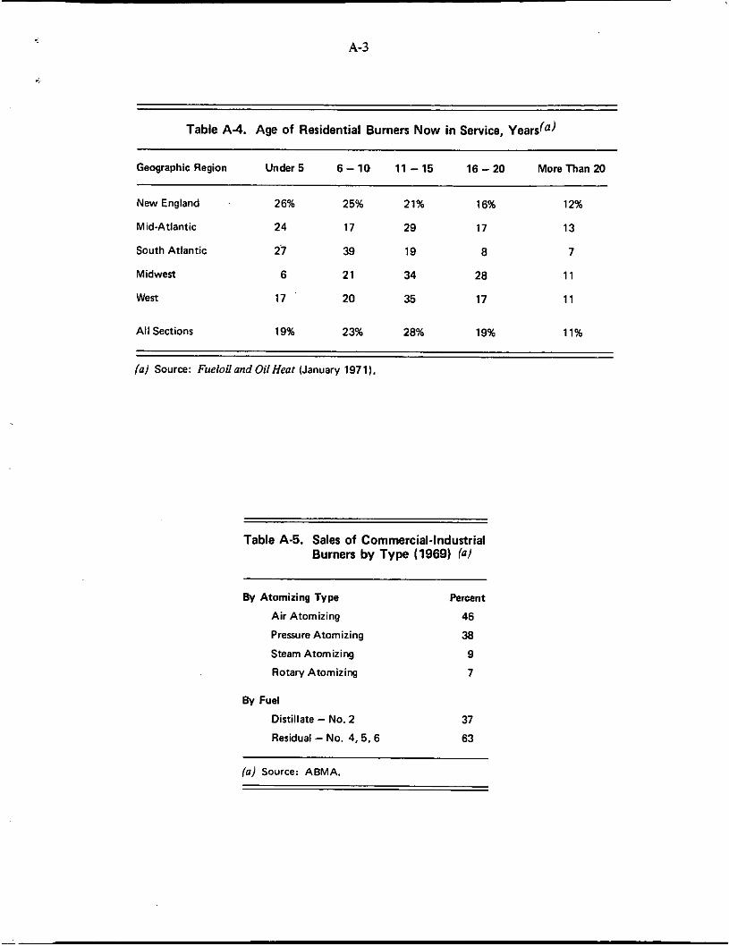
A-3

Table A 4 Age of Residential Burners Now in Service, Years(a)

Geographic Region Under 5 6-10 11-15 16 - 20 More Than 20

New England 26% 25% 21% 16% 12%

Mid-Atlantic 24 17 29 17 13

South Atlantic 2i 39 19 a 7

Midwest 6 21 34 28 1 1

West 17 20 35 17 1 1

All Sections 19% 23% 28% 19% 11%

Table A-5. Sales of Commercial-Industrial Burners by Type (1969) (01

By Atomizing Type Percent

Air Atomizing 46 Pressure Atomizing 38

Steam Atomizing 9 Rotarv Atomizing 7

By Fuel

Distillate - No. 2 37 Residual - No. 4,5. 6 63

(0) Source: ABMA.

5 1

APPENDIX B

FUEL ANALYSES

Residential Fuels

Table B-1 Lists properties of the No. 2 oils fired in residential units for this investigation. Also shown for comparisons are data from the Bureau of Mines fuel survey in terms of average, minimum, and maximum values for each fuel property for fuels marketed in the Eastern Region.(l8)

Table B-2 reports results of chemical analyses for C, H, and N contents of each of these residential fuels.

Commercial Fuels

Table 5 3 lists the generally reported properties for the fuel oils fired in the commercial boilers. These include fuel grades No. 2, 4, 5 , and 6.

Table B-4 reports results of chemical analyses for C, H, and N contents of the commercial fuels.

(18) Shelton, E. M., Burner Fuel Oils, 1971, U. S. Dept. of Interior, Bureau of Mines, Petroleum Products Survey No. 71, August, 1971, p 19.


B-2

I

d

2 - h

c h

d

9 w 9 m - X & ? & $ m N - h N o w m m h ” - - e - I N ? ? * ! 1 q - r - z x z x g 0 0 0 0 0 0 0 0 0 0 0 0 0 0 0 0 0 0 0 0 0 0 0 0 0

9 z 8 8 8 - - -

- x ( 0 - 9 - 9 9 N N N

N

N 10.

h N

N N NLD

m o o Z R ;

Y ” ” N - n n o o - o n n n n

m n N m - - 0nFi n o n

c

n o

2 F:

B-3

Table 8-2. Chemical Analyses of Residential Fuels(0)

Weight Percent Fuel Fired in Unit d b J nib) N ~ C J

1 87.2 2 87.0 3 87.0 4 86.9 5 87.2

6 87.1 7 86.8 8 87.4 9 87.7

10 87.2

11 87.2 12 87 .O 13 87 .o 14 87.3 15 87.4

16 87.2 17 87.2 18 87.1 19 87.1 20 87.0

o(dJ 87.0 &) 86.8

12.5 12.8 12.9 12.8 12.8

12.7 12.6 12.2 12.0 12.3

12.3 12.6 12.2 12.4 12.6

12.5 12.2 12.6 12.6 12.8

12.9 13.2

0.05 0.03 0.03 0.04 0.06

0.05 0.04 0.04 0.03 0.05

0.05 0.03 0.05 0.04 0.03

0.03 0.04 0.05 0.05 0.06

0.07 0.05

(a) Analyses by Battelle-Columbus Analytical

( b ) Reg1 method.

(cJ Kjeldahl method.

( d ) Fuel used in instrument check-out runs at Battelle-Columbus.

(el Reference fuel - a high-quality hydrotreated fuel.

Laboratory.

B-5

Table 8-4. Chemical Analyses of Commercial Fuels(a1

Fuel Weight Percent Fuel Fired Grade,

in Boiler NO. Clbl ~ ( c )

ClOOl C1001’(d)

c1 W2 c1002s1 c1002 52 c1002s3

C1003 c1 OOddJ

C1005

C1006

C1 W7

ClW8

2 2

A

2

4

5

85.4 11.1 0.40 85.4 11.0 0.39

86.2 11.4 0.31 86.6 12.4 0.19 87.0 11.7 0.20 85.1 11.2 0.37

87 .O 12.8 0.05 86.3 12.5 0.04

86.0 11.6 0.25

87.0 . 12.7 0.07

86.0 11.6 0.25

85.9 11.3 0.27

(a) Analyses by Battelle-Columbus Analytical Laboratory. (b) Pregl method.

(e) Kjeldahl method.

(d) Shipment of oil delivered during measurements.

C- I

APPENDIX C

DETAILS OF FIELD PROCEDURES

Residential Units

Prior to setting up the monitoring equipment in the field, each homeowner was visited by a Battelle staff member in advance of the scheduled arrival of the field team. During this visit, the heating unit was examined for accessibility, space requirements, and material needs for rerouting the flue pipe to accommodate the particulate sampling equipment.

The monitoring instruments were set up and recalibrated at each site. Any stack changes were made at this time and the test section of duct (needed for particulate sampling) was placed in the stack. The gaseous sampling trains were set up and the instruments checked out. Stack velocities were measured with an S-type pitot tube; flue-gas flow rate and excess air were calculated. Pressure and temperature measurements were made, and the fuel rate determined volumetrically by connecting the pump suction to a calibrated container and timing fuel consumption.

After all the instruments were operating correctly and leak checked, a firing cycle of 10 minutes on and 20 minutes off was established by by-passing the thermostat with an automatic timer.

Measurements were made of the following stack emissions under various conditions of operation:

c 0 2

0 2

so2

co

NOx and NO2 (NO obtained by difference)

Hydrocarbons (total)

Particulate loading.

In addition to these measurements, the combustion conditions normally observed by servicemen were measured. These conditions included: draft (over-fne and stack), flue-gas temperature (at the sampling point) - plus smoke, C02, and 02 as measured by standard field-type instruments.

Sampling of stack gases from the heating unit was done directly, with a sample fed to continuous monitoring equipment set up near the oil-burner unit. Details of instrumentation and measurement procedures are described in Appendix D and E.


c-2

Emissions from residential units were monitored under the following sets of conditions:

(1) The as-found condition

(a) cold start, C (b) warm, after repeated cycles, - A

(2) A tuned condition,

(3) Firing a No. 2 hydrotreated reference fuel, R. -

As-Found Condition. The initial tests on the heating unit were made in the “as-found” condition, Le., no servicing or changes were made except for the rerouting of the flue pipe. The first cycle was made from a relatively cold start, generally after a minimum 60-minute off period. Gaseous-emission measurements were made for the entire period, including both the on and off portion of the cycles. Particulate measurements were started at the beginning of the second cycle and measured during each 10 minutes firing portion of four or five additional cycles. A total of SO to 60 minutes of firing time (about 3 hours elapsed time) was required for the particulate sampling.

Tuned Condirmn. Following the test run in the “as-found’’ condition on 18 of the units, the serviceman cleaned and tuned the burner. This was not an “eye-ball” adjustment, but it was intended to be a tuning that a skilled serviceman would achieve with normal procedures of good practice with the benefit of instrument readings of draft, C02, and smoke. The following steps were included in the serviceman’s procedure to establish the tuned condition.

Cleaning and adjusting the electrodes

Cleaning the blast tube and blower wheel

Cleaning or replacing the nozzle (even by a different size or spray

Cleaning or replacing the oil fiter

Simple sealing of air leaks at inspection door, around blast tube, or in other easily accessible locations

Change in draft-regulator setting (replaced regulator when necessary)

0 Change in combustion air adjustment.

pattern if it were better suited to the installation)

The following items, being major repairs or modernization requiring special charges to the homeowner, were not - included in the serviceman’s procedure.

Replacement of the combustion chamber or liner

Replacement of the combustion head

Seaiing of air leaks that would require disasasrnbly o l the boiler or furnace jacket.


->

c-3 -1

The field team developed a rough C02-smoke curve as part of defining the well-tuned conditions. The air adjustment was then made just off the “knuckle” of this curve. The instructions for adjusting to the tuned condition consisted of these steps:

( I ) Compare the CO? level in the stack with that obtained in sampling by traversing above the fire using a simple averaging procedure. An appreciable difference between stack and over-fire C02 is indicative of air infiltration through leaks; easily accessible leaks are to be repaired.

(2) Establish a smokeC02 curve by use of the continuous C 0 2 reading and the Von Brand smoke trace (with only enough points to define the general shape, and particularly the location of the “knuckle”).

(3) I f No. 1 or less Bacharach smoke can be achieved with air adjustment alone, adjust the burner t o the maximum C02 for No. 1 smoke, but allowing a cushion no nearer the “knuckle” than 0.5 to 1.0 percent C02. (It would be expected that a well-tuned burner should operate with at least 8 percent C02).

(4) If Step (3) cannot be accomplished to reach a No. 1 smoke, carry out any of the specific tuning steps listed above to achieve that performance, or approach it as closely as possible. In this procedure, first priority should be given to reducing smoke level t o at least No. 2, and second priority to maintaining high C 0 2 (with 0.5 to 1 .O percent cushion from the “knuckle”). The smokeC02 curve should be repeated to define the burner performance and to locate the desired setting for the tuned test run.

Table C-l shows the steps in tuning the residential units. All the units were tuned except for Units 6 and 19. Unit 6 was serviced 3 weeks prior t o testing, and Unit 19 presented excessive difficulties in tuning.

Gaseous emissions were measured on all tuned units but data was not recorded for four units where tuned data appeared identical to as-found data. Particulate was measured when appreciable change in smoke or emission data were observed from the as-found condition.

Reference Fuel. After completing the tests for the as-found and tuned conditions, each residential unit was operated for a short period of time on a reference fuel; and gaseous emissions and smoke were measured during the I O minutes 0 4 2 0 minutes off cycle. The reference fuel was a high quality No. 2 hydrotreated fuel. The purpose of the reference fuel measurements was to provide a baseline in comparing the variety of burner units on a common fuel basis and, thus, to remove the effect of randomness in the quality of house fuels.

Commercial Boilers

Although the instrumentation techniques and the emission measurements used for the commercial boilers were similar to those employed for the residential units, the conditions under which the measurements were made were quite different.


c-4

Table C-1. Information on Condition and Tuning of Residential Units

Normal . . . Atomizing Nozzls Cleaning &

size. Renun. psi Electrode Unit Iph Cleaned Replaced &.Found Tuned Adi. other step* Remarks

1.35

2 1.00

3ia1 3.00

4 1.25

X - - X

X

- X

-

Good condition

Good Condition

Average condition

Very old unit. with cracks in combustion chamber: p w r condition. dirty house fuel.

very old uni1:yellw make spot: p w r condition: unburned fuel in Rack: hould be replaced.

Excellent condition: cleaned and serviced 3 weeks prior to test

12-year old Combustion chamber. could not tune properly: poor condition

Leak in v z w m side of fuel wrtern. could not repair: mod condition.

Good condition

Average condition: very old bailer.

Good condition.

Average condition.

Average condition.

Average condition.

Average condition.

Cleaned pump filter

- Replaced draft damper

d") 1.25 - X X Resealed combustion chamber door

db) 1.35 1 w

71a/ 2.50 - X X Replaced fuel filtei

8 1.50 - X 95 105

-

X

9 3.25

l e 2.50

X - X -

100

120

X

X

11 0.50

12 1.w X - - X

90

1W

X

X Replaced fuel pump filter

13 1.25

14 1.35

- X

X - 110

185

90

105

X

X Replafad fuel pump wring and bellows

Replaced fuel pump filter: cleaned chimney base

Replaced fuel pump filter and g d e t and oil filter

Replaced blast tube. draw arrembly. filter and pump filter

15 3.50 - X 1W X

16 1.75 X - 100 X Good condition

17 2.50 X - 90 X Soot accumulation in flue p-: removed side panels and cleaned bailer tuber:

chimney base: good condition

h u t down: could not repair: average condition

resealed panel% cleaned

Fuel after drip when burner

Unit 1w1 not 1uned:adiust.

Yellow smoke Ipot: owner

men1 difficultia

witched from No. 1 to NO. 2 fuel 2 months before without adjusting burner: unburned fuel in stack: this unit w- tuned and adiusted on NO. 1 oil: flame pattern indicated air leaks around heaRh

18 1.35 X - 80 1w X Removed obstruction from chimney

19fbJ 12.1)

20 (0.6) Removed and cleaned grills: cleaned chimney chimney base

fa/ Unit tuned. but no emission data taken owing to insignificant change in performance. f b ) Unit not tuned.

c-5 d

The commercial boilers were all investigated in the as-found condition, Le., no cleaning (except for the exhaust stack) or other servicing was done prior to testing. Wherever practical, the exhaust stacks were thoroughly cleaned prior to testing; this cleaning procedure was not economically feasible in three of the units because particulate sampling for two of the units (Boilers ClOOS and C1006) was done from the roof, and the exhaust stack from the third boiler (Boiler ‘21007) was not readily accessible for cleaning.

The commercial measurements were conducted in late spring 1971 (April-May) near the end of the heating season. Visual inspection of the units showed the normal accumulation of soot and ash one would expect to find over a typical heating season.

Emission data from the commercial units were obtained under steady-state conditions at four load levels:

H, - 80 percent of rated load - L, normal low-fire setting

M, - an intermediate load

- T, typical plant or rated load - the generally accepted or established firing rate for the installation.

Each burner was set to operate at 12 percent C02 at the 80 percent load, the conditions established as a baseline after discussions with the ABMA Commercial-Industrial Air Pollution Committee. The normal air-fuel proportioning linkage provided the air adjustment at low fire setting. Since particulate analyses required extensive sampling times (approximately 80 minutes at each load setting), particulates were only obtained at 2 loads: 80 percent and low load. To assure the attainment of steady-state conditions when changing load or excess air, the boilers were operated at the new setting for 30 minutes before particulate sampling was begun.

Boiler C1006 was fired with a burner having a fixed firing rate and was only operated at two load settings: 80 and 100 percent. The two rates were obtained by changing the nozzle size.

The fuel supply used during the sampling runs were those available in the supply tanks at the site at the time of the measurements, the only exception being for one boiler in which three additional residual oil samples were supplied from drums.


D-1

APPENDIX D

SAMPLING AND ANALYTICAL PROCEDURES FOR GASEOUS EMISSIONS

Sampling

Selection of installations with adequate space and accessibility made it possible to sample the gaseous emissions from stacks directly. Direct sampling was accomplished by drilling two holes (1/2 inch in diameter) in the flue pipe and inserting sampling probes with lines leading directly to the monitoring equipment. Direct sampling with the shortest possible lines minimized line losses by condensation, reaction, and/or adsorption.

A schematic drawing of the sampling train used in monitoring gaseous emissions from both residential and commercial units is shown in Figure D-I.

Stack ( A

L w W a t e r traps

Figure P1. Sampling Trains for Gaseous Emissions

Two sampling trains were used, one for S02, NO,, and NO2 and a second for C02, 0 2 , CO, and total hydrocarbons. Each train consisted of a Pyrex ice-water trap (with a side arm sufficiently long to reach the center of the largest flue pipe) and a small glass-wool particulate trap. Teflon lines were used in the first train and a stainless steel manifold with polyethylene lines was used in the second. Figures 1-1 and 1-2 show the instrumentation setup used in the field for residential and commercial units, respectively. .


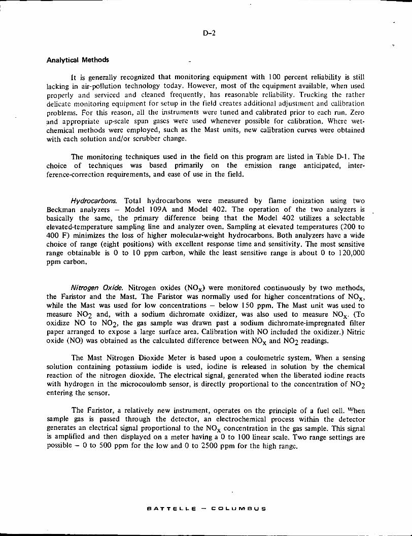
D-2

Analytical Methods

It is generally recognized that monitoring equipment with 100 percent reliability is still lacking in air-pollution technology today. However, most of the equipment available, when used properly and serviced and cleaned frequently, has reasonable reliability. Trucking the rather delicate monitoring eqiiipnirnt for sctup in the field creates additional adjustment and calibration problems. For this reason, all the instruments were tuned and calibrated prior to each run. Zero and appropriate up-scale span gases were used whenever possible for Calibration. Where wet- chemical methods were employed, such as the Mast units, new calibration curves were obtained with each solution and/or scrubber change.

The monitoring techniques used in the field on this program are listed in Table D-I. The choice of techniques was based primarily on the emission range anticipated, interference-correction requirements, and ease of use in the field.

Hydrocarbons. Total hydrocarbons were measured by flame ionization using two Beckman analyzers - Model 109A and Model 402. The operation of the two analyzers is basically the same, the primary difference being that the Model 402 utilizes a selectable elevated-temperature sampling line and analyzer oven. Sampling at elevated temperatures (200 to 400 F) minimizes the loss of higher molecular-weight hydrocarbons. Both analyzers have a wide choice of range (eight positions) with excellent response time and sensitivity. The most sensitive range obtainable is 0 to I O ppm carbon, while the least sensitive range is about 0 to 120,000 ppm carbon.

Nirrogen Oxide. Nitrogen oxides (NO,) were monitored coatinuously by two methods, the Faristor and the Mast. The Faristor was normally used for higher concentrations of NO,, while the Mast was used for low concentrations - below 150 ppm. The Mast unit was used to measure NO2 and, with a sodium dichromate oxidizer, was also used to measure NO,. (To oxidize NO to NO2, the gas sample was drawn past a sodium dichromate-impregnated filter paper arranged to expose a large surface area. Calibration with NO included the oxidizer.) Nitric oxide (NO) was obtained as the calculated difference between NOx and NO2 readings.

The Mast Nitrogen Dioxide Meter is based upon a coulometric system. When a sensing solution containing potassium iodide is used, iodine is released in solution by the chemical reaction of the nitrogen dioxide. The electrical signal, generated when the liberated iodine reacts with hydrogen in the microcoulomb sensor, is directly proportional to the concentration of NO2 entering the sensor.

The Faristor, a relatively new instrument, operates on the principle of a fuel cell. ?!hen sample gas is passed through the detector, an electrochemical process within the detector generates an electrical signal proportional to the NOx concentration in the gas sample. This signal is amplified and then displayed on a meter having a 0 to 100 linear scale. Two range settings are possible - 0 to 500 ppm for the low and 0 to 2500 ppm for the high range.


D3

Table D-1. Gaseous Emission Instrumentation Used in Field Survey

Pollutant lnnrument Rangefa) Principle of Operation Comments

Beckman Model 109 0120,000 Beckman Model 402 0120.000

Varian HiFi 111 Variable

Faristor 02500

Mast 0.1-200

Mast 05000

Faristor 02500

Beckman Model 215A 0-600

MSA, Model 300 020%

Beckman Model 215A 020%

Beckman Model 715 025%

Flame ionization Flame ionization

Gas chromatography

Electrochemical (dry)

Electrochemical (wet)

Electrochemical (wet)

Electrochemical (dry)

NDlR

NDlR

NDlR

Amperometric

Continuous, fast response, portatile Selectable elevated temperature

C2C6, choice of solumns, semi- sampling line and oven

portable batch operation

Continuous, fast response, portable; SO2 interference can be accommodated

Continuous, fast response, portable; NO oxidizer and SO2 correction required

Continuous, fast response, portable; SO2 correction required

Continuous, fast response, portable; no NO2 interference

Continuous, portable; water and C02 interference can be accommodated

Continuous, portable; water interference can be accommodated

Continuous, portable; water interference can be accommodated

Continuous, portable

fa) ppm except as noted.

I

D-4

SuZfur Dioxide. The Faristor was also used to measure SO2. The series NS-200 SO2/ Nitrogen Oxide Analyzer operates in the bimodular mode using two Faristor plug-in detectors, Type N76H2 for measuring NOx and Type S64H2 for measuring SO2. Two analog outputs are available on the Faristor which permits simultaneous monitoring of both gases.

Carbon Monoxide. Carbon monoxide was continuously monitored by nondispersive infrared, using a Beckman Model 215A analyzer. The instrument has three ranges. Range 1 is 0 to 250 ppm, and Ranges 2 and 3 have adjustable ranges to 600 ppm. The sensitivity is 0.5 percent of full scale with an accuracy of ? I percent.

Carbon Dioxide. Nondispersive infrared was also used in monitoring CO2. The instrument, a Beckman Model 215A, has two ranges (0 to 5 percent and 0 to 20 percent CO2 by volume). The sensitivity is 0.5 percent of full scale with an accuracy of ?I percent on Range 1 and t 2 percent on Range 2.

Oxygen. The Beckman Model 715 Rocess Oxygen Analyzer was used to continuously monitor gaseous oxygen. The analyzer has ranges of 0 to 5 percent and 0 to 25 percent oxygen. Sensor response is 90 percent of full scale in less than 20 seconds.

The amperometric oxygen sensor contains a gold cathode and silver anode. The two electrodes are separately mounted within the PVC body, and are electrically connected by a potassium chloride electrolyte. A gas-permeable Teflon membrane separates the electrodes from the process sample and fits fumly against the gold cathode. Oxygen from the sample diffuses through the membrane and is reduced at the gold cathode. The resultant electrical current flow between the electrodes is proportional to the partial pressure of oxygen in the sample.

Interpretation of Cyclic Data, Instantaneous Versus Average Values

The instruments for measuring CO and HC had fast response times, essentially instantaneous values of emission concentrations of these gases were obtained - including peaks at startup and shutdown. Table D2 provides a comparison of two instantaneous values (5th minute and 10th minute) and dose average values (obtained by dividing the area under the ppm versus time curve by the cycle length). The differences between these values are generally small, but the dose average values were used in calculating emission factors for CO and HC.

Due to time-lag in the instrumentation, instantaneous values could not be obtained for S02, NO,, and N02. Therefore, these emission factors were calculated on the basis of the 10th minute emission measurements.


D-5

Table D-2. Carbon Monoxide and Hydrocarbon Emissions - Comparison of Instantaneous and Average Values for Residential Units

CO, ppm HC. ppm Unit Condition 5th min 10th min Dose Avq. 5th min 10th min Dore Avg.

1

2

3

4

5

6

7

8

9

10

C A T R

C A T R

C A T R

C A T R

C A T R

C A T R

C A T R

C A T R

C A T R

C A T R

12.5 10.5 8.9 9.5

6.3 5.8

37.5 35.5 22.5 19.1 26.7 26.7 24.5 26.8

- 15.0 18.7 19.1

4.5 5.2

- -

- -

- - 18.0 25.1 55.9 37.7 41.1 25.6

> 250.0 > 250.0 > 250.0 >250.0

> 250.0 >250.0

10.7 8.4 10.7 10.4

13.1 11.9

4.2 4.2 5.7 6.1

0.5 0.5

16.7 12.7 13.0 12.9 10.0 9.5 12.5 9.5

4.2 4.2 10.0 9.5 7.5 7.9 7.0 6.3

- 7.5 9.5 8.4 5.0 4.5 6.7 6.4

- -

- -

- -

16.9 14.3

10.7

42.4 23.8 36.1 34.9

-

- 20.2

5.1

-

- 19.2 72.7 58.4

> 250.0 > 250.0

>250.0

10.8 12.7

17.2

6.3 7.3

2.8

17.7 14.8 9.6

14.8

7.0 10.4 8.3 7.3

-

-

-

- 9.8 5.8 7.0

4.0 2.8

4.0

5.5 3.3 3.4 4.7

-

- 2.2

0.8 -

- 1.1 3.8 2.3

265 277 -

52.3

3.0 2.9

4.0

2.5 1 .8

2.7

-

-

- 3.7 1.9 4.5

4.4 4.5 2.7 2.2

4.8 5.1 6.7 7.1

3.5 2.6

3.2

5.2 3.4 4.3 4.7

-

- 0.3

0.7 -

- 1.9 4.1 2.4

235 247 -

49.7

3.2 3.2 - -

1.5 2.1

2.6

-

- 3.8 1.9 4.3

4.4 5.7 2.7 1.7

5.0 5.2 6.7 7.2

5.1 3.0

5.2

6.7 4.8 4.5 5.5

-

- 3.8

0.9 -

- 1.3 4.4 2.8

258 268

- 50.2

3.4 3.5 - -

2.7 2.5

3.6

-

- 3.8 2.1 5.8

4.7 5.9 3.0 2.9

5.1 5.2 6.9 7.3

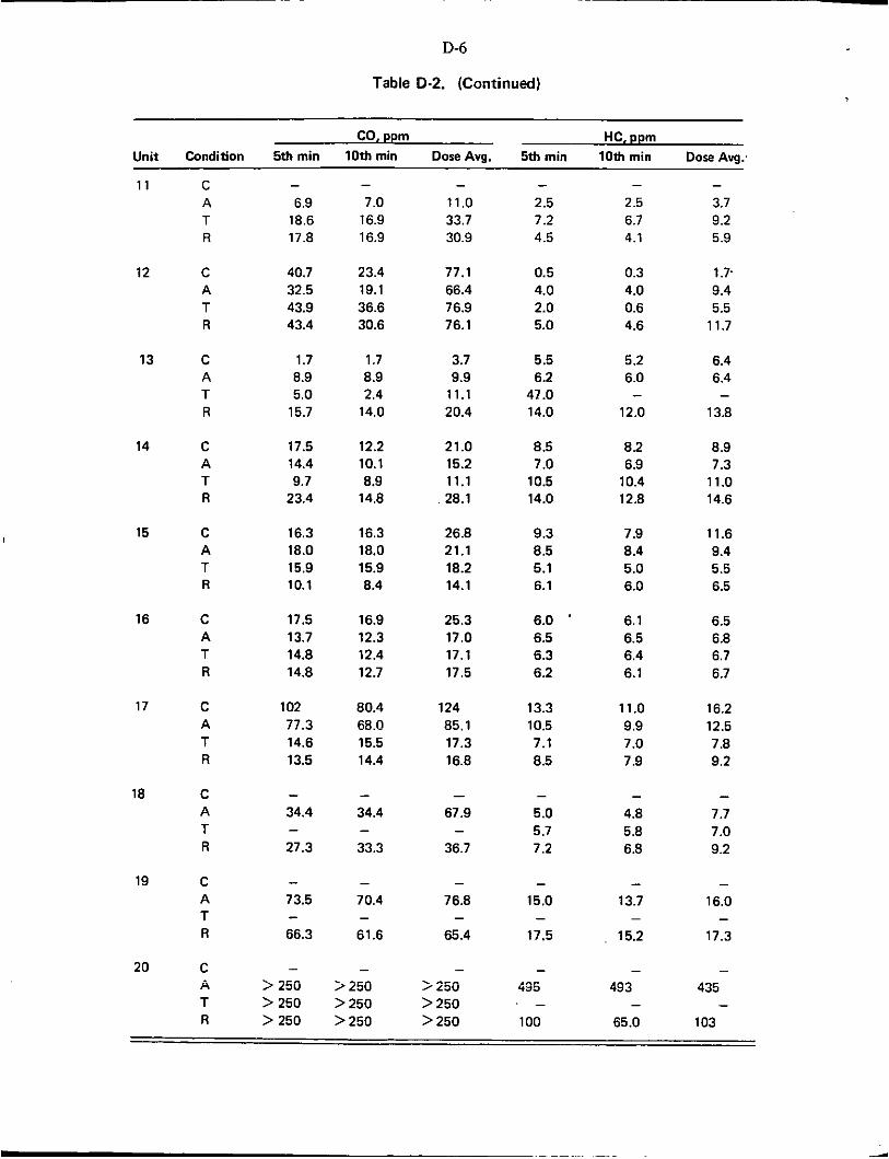
D-6

Table D-2. (Continued)

CO, ppm HC, ppm

Unit Condition 5th min 10th min Dose Avg. 5th min 10th min Do= Avg.

11

12

13

14

15

16

17

18

19

20

C A T R

C A T R

C A T R

C A T R

C A T R

C A T R

C

T R

C A T R

C A T R

C A T R

A ..

- 6.9

18.6 17.8

40.7 32.5 43.9 43.4

1.7 8.9 5.0

15.7

17.5 14.4 9.7

23.4

16.3 18.0 15.9 10.1

17.5 13.7 14.8 14.8

102 77.3 14.6 13.5

- 34.4

27.3

-

- 73.5

66.3 -

- > 250 > 250 > 250

- 7.0

16.9 16.9

23.4 19.1 36.6 30.6

1.7 8.9 2.4

14.0

12.2 10.1 8.9

14.8

16.3 18.0 15.9 8.4

16.9 12.3 12.4 12.7

80.4 68.0 15.5 14.4

- 34.4

33.3

-

- 70.4

61.6 -

- > 2% > 250 > 250

- 11.0 33.7 30.9

77.1 66.4 76.9 76.1

3.7 9.9

11.1 20.4

21.0 15.2 11.1 28.1

26.8 21.1 18.2 14.1

25.3 17.0 17.1 17.5

124 85.1 17.3 16.8

- 67.9

36.7

-

- 76.8

65.4

-

- > 250 > 250 > 250

- 2.5 7.2 4.5

0.5 4.0 2.0 5.0

5.5 6.2

47.0 14.0

8.5 7.0

10.5 14.0

9.3 8.5 5.1 6.1

6.0 '

6.5 6.3 6.2

13.3 10.5 7.1 8.5

- 5.0 5.7 7.2

- 15.0

17.5 -

- 435

100

. -

-

2.5 6.7 4.1

0.3 4.0 0.6 4.6

5.2 6.0

12.0

8.2 6.9

10.4 12.8

7.9 8.4 5.0 6.0

6.1 6.5 6.4 6.1

11.0 9.9 7.0 7.9

-

- 4.8 5.8 6.8

- 13.7

15.2

-

- 493

65.0 -

- 3.7 9.2 5.9

1 .? 9.4 5.5

11.7

6.4 6.4

13.8

8.9 7.3

11.0 14.6

11.6 9.4 5.5 6.5

6.5 6.8 6.7 6.7

16.2 12.5 7.8 9.2

-

- 7.7 7.0 9.2

- 16.0

17.3 -

- 435

103 -

n 7

Measured HC Levels Compared to Ambient Levels

Table D-3 provides a comparison of the measured HC emission concentrations (at the 10th minute point for the as-found condition) and the ambient HC concentrations in the basement near the furnace and in the stack after the unit has been off for at least one hour. These data show that the residential units actually reduced HC levels below the intake air in some cases. It should be noted that the ambient HC levels in the basements were somewhpt higher than normally measured for outdoor ambient levels because of oil spillage which occurred when disconnecting oil lines to measure fuel firing rates.

Table 0-3. Total Hydrocarbons for Residential Units

HC Concentration, ppm Room Flue &-Found,

Unit Ambient(a) Ambient fa) 10 min.

1 2 3 4 5

6 7 8 9

10

11 12 13 14 15

16 17 18 19 20

5.2 4.0 3.4 0.9 2.3

4.4 3.4 5.0 4.6 5.7

- 3.2 5.0

10.0 7.0

6.8 6.0

5.2 10.5

-

5.5 3.5 1.5 1.4 2.5

4.2 3.6 4.5 4.8 6.3

1.7 4.0 5.0

10.2 6.6

6.8 6.7 4.8 5.2

10.2

2.6 3.4 0.3 1.9

247.0

3.2 2.1 3.8 5.7 5.2

2.5 4.0 6.0 6.9 8.4

6.5 9.9 4.8

13.7 493.0

fa) "Room ambient" and "flue ambient" data obtained prior to cold start condition.

E- I

APPENDIX E

SAMPLING AND ANALYTICAL PROCEDURES FOR PARTICULATE AND SMOKE

PARTICULATE SAMPLl NG

The particulate sampling rig used in th i s investigation was the EPA or APCO sampling train, with modifications for oil burner emissions measurements. Figure E-1 shows the particulate sampling train. For the residential runs, the sampling probes used were a combination nozzle and probe 12 and 15 inches long extending out of the top of the heated chamber of the sampling train. The cyclone included in the EPA rig was not used and the probe was connected directly to the filter. For the commercial runs, a 36-inch combination probe and nozzle was used and the cyclone was used. The rest of the train was as shown in Figure E-1, and the procedures of operation (except probe and impinger washing) were those specified by EPA publicationsll 1,12)

Velocities in the stacks were measured by S type pitot tube. However, it was not always possible to get a reliable velocity pressure reading readily, as some flue gas velocities were so low that the pitot tube velocity pressures were in the range of 0.002 to 0.005 inch of water. To insure isokinetic sampling, it was necessary to check these measurements with the calculated flows from the fuel feed rate and the excess air.

As the firing o! the residential units is relatively constant during the 10-minute fning period, S-type pitot tube measurements were made during the cycles preceding the beginning of sampling. Temperatures were measured both before and during the runs. For sampling from commercial boilers, the S type pitot tube and thermocouple were attached to the probe and positioned adjacent to the sampling nozzle. In all cases, fuel41 firing rate was measured previous to the run. Excess air was determined and the flue-gas volume and average velocity were calculated and compared with the pitot tube measurements to assure isokinetic sampling.

In cases where the velocity profile across the duct was relatively uniform, the sample was collected by isokinetic sampling at a velocity about equal to the average velocity. Sampling at the average velocity was not possible where velocity profiles were not uniform.

The sampling rig was operated in accord with the EPA (APCO) recommendation, Le., the filter was kept at a temperature between 230 and 250 F and the impingers were kept in an ice bath. The first two impingers contained 100 ml of double-distilled water each, a third impinger was initially dry and the fourth impinger contained about 175 grams of Drierite. Moisture was collected in the impingers and in the Drierite. The dry flue gas was measured by a dry gas meter during the run.

Before the sampler was put in operation, it was leak-checked to see that all the joints were tight. The nozzle was plugged with a rubber stopper and 10 inches of vacuum was placed on the system. With this vacuum, no more than 0.02 cubic foot leakage was permitted; checks showed this usually was much less than this value.


E-2

Probe Filter Impingers I

A I

1.

2. 3.

4.

5 . 6. 7.

8.

9. IO.

\ W a t e r bubblers

19

Stainless steel, buttonhook-type probe tip Stainless steel coupling Robe body, S/S-inch OD, medium-wall &rex tubelogarithmically wound with 25 feet 26 ga. nickel-chromium wire Cyclone and flask (not used for residential units) Fritted-glass filter holder Electrically heated enclosed box Ice bath containing four impingers connected in series The Greenburg-Smith type impinger with tip removal Second impinger with tip

Third impinger with tip removed

1 I . Fourth impinger with tip removed and containing approximately 175 grams of accurately weighed dry silica gel

12. Pressure gauge 13. Checkvalve 14. Flexible-rubber vacuum tubing 15. Vacuum gauge 16. Needle valve 17. Leakless vacuum pump 18. By-pass valve 19. Dry-gas meter 20. Calibrated orifice 21. Draft gauge

22. S-type pitot tube

Figure E-1. EPA or APCO Particulate Sampling Train

‘1

E-3

Silver membrane filters were used. The filter for the residential unit was a 3-inch diameter silver membrane with a pore size of 0.8 micron. Because of the higher loadings for the commercial units, a larger 5-inch-diameter silver membrane filter with a pore size of 0.8 micron was used in those cases.

For the residential units, particulate sampling was initiated just before the IO-minute “on” cycle started and was stopped just after the burner was shut down. During the 20-minute. “off’ cycle, there was no particulate sampling. Five or six firing cycles were required to collect sufficient particulate catch for weighing and analysis.

\

PARTICULATE ANALYSIS

Moisture Content

After the particulate run was completed, the moisture content of the sampled gas was determined as follows: the Drierite was weighed to determine the gain in weight and the amount of moisture in each of the impingers was measured. These measurements were accumulated to obtain the total increase of water in the system and the moisture content of the flue gas calculated.

Particulate Loading

The silver membrane filters were dried and the tare weight obtained before the run was started. After the run was made, the filter was removed, dried, desiccated, and weighed t o obtain the quantity of material collected on the filter.

The internal parts of the sampling probe nozzle and connecting tubes plus the first half of the filter holder were washed with water, acetone, and methylene chloride, and again with acetone.* The glassware including, the last half of the fdter holder and the three impingers were washed with the water in the system, then with acetone, with methylene chloride, and with a final acetone wash.* The wash fractions were separated in each of these stages into two jars and sealed and labeled for analysis.

One-half of the probe wash and of the impinger solution was dried and weighed as shown in Figure E-2 to determine the weight of particulate collected.

*The EPA procedure (References 11 and 12) specifies washing the probe with acetone and the impinger with water and acetone. Experience at Battelle has shown that this is not sufficient to wash all material from the probe and impinger surfaces.


Water portion methylene

Evaporate visible water at 212 F

Dry in - air

Desiccate at room temperature for several days

Weigh

Figure E-2. Drying Procedure for Probe and lrnpinger Washes

As the result of work on another project being conducted at BattelleColumbus under EPA contract, questions have arisen as to whether the samples are really dry after using the procedure shown in Figure E-2. Therefore, several probe and impinger samples were dried by an additional and more extensive procedure. This additional procedure, and the sample weights obtained at each step, are shown in Table E-I. The additional drying caused a weight change in the probe samples of from +I3 percent to -24 percent, this was not a substantial change. However, the weight of the impinger samples decreased by from 32 to 56 percent, quite a substantial change.

Although the exact nature of the material driven off in this drying is not known, it is suspected to be primarily water. However, the slow changes in weight, both positive and negative, that occurred during extended periods of dessication and heat treatment imply that the weight changes may not be due to changes in free water content alone, but also due to some uncertain chemical changes involving sulfates, organics, and possibly carbonates and nitrates. More extensive research is urgently needed to establish reproducible methods for determining dried sample weights and composition. Meanwhile, it is believed that the results tabulated in this report are consistent with the EPA method and are meaningful within the limits of the present state of the art of particulate sampling and analysis.


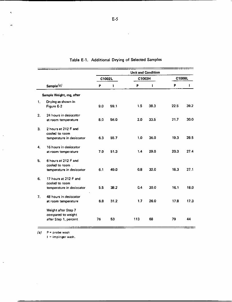
Table E-1. Additional Drying of Selected Samples

Unit and Condition

C1002L C1003H C1008L

Sampleia) P I P I P I

Sample Weight, mg, after

1. Drying as shown in 9.0 59.1 1.5 38.3 22.5 39.2 Figure E-2

2. 24 hours in desiccator a t room temperature 8.0 56.0 2.0 33.5 21.7 30.0

2 hoursat 212 F and cooled to room temperature in desiccator 6.3 55.7 1.0 36.0 19.3 28.5

3.

4. 16 hours in desiccator a t room temperature 7.0 51.3 1.4 29.0 20.3 27.4

6 hoursat 212 F and cooled to room temperature in desiccator 6.1 49.0 0.8 32.0 18.3 27.1

17 hours at 212 F and cooled to room temperature in desiccator 5.5 38.2 0.4 30.0 16.1 18.0

5.

6.

7. 48 hours in desiccator at r m m temperature 6.8 31.2 1.7 26.0 17.8 17.3

Weight after Step 7 compared to weight after Step 1. percent 76 53 113 68 79 44

fa) P = probe wash I = impinger wash.

E-6

Other Analyses

Some of the particulate samples were analyzed for polynuclear aromatics (PNA) as benzo-a-pyrene (BaP), C-H-N content, and metals. For these samples, the acetone and methylene chloride used were high-purity distilled-in-glass chemicals. All the liquid samples were stored in glass jars with Teflon sealed caps. For shipping to the lab, the filters and solution were kept cool in an ice chamber and were refrigerated at the lab so that loss would be minimum in transit and in storage.

The procedure developed for analysis of the particulate samples is outlined in Figure E-3. The evaporations were carried out in 80 x 45-mm Pyrex evaporating dishes and the residues were weighed as collected in these dishes.

PNA. For the benzo-x-pyrene analysis, one-half of the filter was combined with one-half of both the probe wash and the impingers wash. BaP was analyzed by using high-pressure liquid chromatography and checked with thin layer chromatography.

The BaP analysis is substantially that published in Heulrh Luborufory Science, I, 56-9, January Supplement (1970) in which the BaP is separated from most other organic material by TLC and then analyzed by fluorescence at the H i s 0 4 salt of BaP.

C-KN. One-quarter of the filter material and aliqouts of the probe and impinger collections were analyzed for C-H-N and also the benzene soluble portion of the C-H-N. For the C-H-N analyses, the residue samples were reslurried in ethanol and then evaporated to deposit them in suitable small platinum boats.

Six samples were heated in air at 750 F to obtain an estimate of the weight fraction of the sample that can be volatilized or combusted.

Metals. Another quarter of the fiiter and aliqouts of the probe and impinger collections were used for the metal identification by optical emission spectrometry. The optical emission spectrosLuyic analyses were made on I cm2 portions of the silver filtcr bearing corresponding portions of the particulate collection. Standards were made by mixing metal salts with pure silver powder. Metals analyzed by optical emissions spectrometry were those metals that were detect- able.

Particle Sizing

Particle-size measurements were made for one commercial boiler run. The Battelle Cascade Impactor provided a method for classifying particles into 6 sizes. 0.2 p, 0.4 p, 0.9 p, 1.8 p, 3.5 /A, and 7.0 p. The design of the impactor is based on the principle of particles in a moving aerosol impacting on a slide placed in the air stream. If a particle is sufficiently large it will impact; the smaller particles will continue to travel around the slide to the next stage. The jet diameter of each succeeding stage decreases. Thus, the particle will increase in velocity until it ubiaiiis suffide;lii iiteriia tu impact as illustrated ili Figure E-4( 19).

(19) Pilcher, J . M., Mitchell, R. I . , and Thomas, R. E., ‘The Cascade Impactor for ParticlsSize Analysis of Aerosols”, Resented to the Chemical Specialists Manufacturers Assoc., Inc., New York City, December 6 and 7, 1955.


',

E-I

U I

U

E-8

First Stage: Large jet Low velocity Large particles impact

Succeeding Stages: Smaller jets Higher velocities Smaller particles impact

Figure E-4. Schematic Diagram Showing Principle of the Cascade Impactor

E-9

Several tests were required to determine the length of sampling time required to.obtain a sample of measurable weight for this analysis. In addition, calculations were made to determine proper nozzle size to meet isokinetic conditions. These preliminary runs were made on glass slides. Silver membrane filters, 25 mm in diameter were used to collect the actual sample. A glass slide backing acted as support for this material. Because of the small weight gain involved, the silver membrane, with a relatively small tare weight, provided a more reliable method of collection than would have the stmdard glass slide only. Sampling time for unit C1002-S3 was two minutes a t a fixed flow rate of 0.023 scfm. To prevent disturbances in air flow caused by the impactor in the stack, the nozzle was displaced 12 inches ahead of the first stage.

Prior to inserting the impactor into the stack, it was heated to stack temperature to prevent moisture from condensing in the impactor. Although the dewpoints of many substances in flue gas are below stack temperature, it was felt that impaction at this temperature would minimize the possibility of obtaining false size distribution. If a particle enters the impactor when moisture is present, it may become the nucleus of a moist droplet and impact as a larger size particle.

SMOKE SAMPLING TECHNIQUES

Two techniques of sampling smoke were used. The standard Bacharach hand-pump smoke meter was the primary method of spot sampling. In some instances, Bacharach smoke readings were made at the I-minute, 5-minute, and 9-minute points of the “on” cycle. As expected, the smoke number decreased as the cycle proceeded. The decrease between the 1 and 5-minute points was much greater than that between the 5 and 9-minute points. (By the 5-minute point, the stack had reached approximately 80 percent of its steadystate temperature.)

The ports used for the gaseous measurements generally served as sampling locations for smoke measurements. If conditions suggested erroneous readings due to greatly disturbed air flow, the sample was taken through the particulate sampling port. However, in most cases, the gaseous ports were adequate.

To monitor the variations in smoke as the cycle progressed, a Von Brand continuous recording smoke meter was used. Readings were obtained by using the Von Brand reflectometer. During a run, the vacuum pump was started 15 seconds prior to ignition. This permitted ambient stack air to be recorded prior to the “on puff”. The equipment was sampled continually throughout each on-cycle until all evidence of the “off puff’ ceased. The length of the “off puff’ varied from 1 second to 30 seconds. The “on- and off-puffs’’ coincide with the CO and HC peaks noted for the gaseous emissions (see Section IV, Figure IV-1).

A Photovolt reflectometer with tri-color filter was used to assist evaluation of Bacharach smoke readings on the commercial boilers. This provided a means of accurately reading the smoke spot while reducing the possibility of human error caused by inadequate lighting or yellow sulfurous material or oil on the smoke spot.


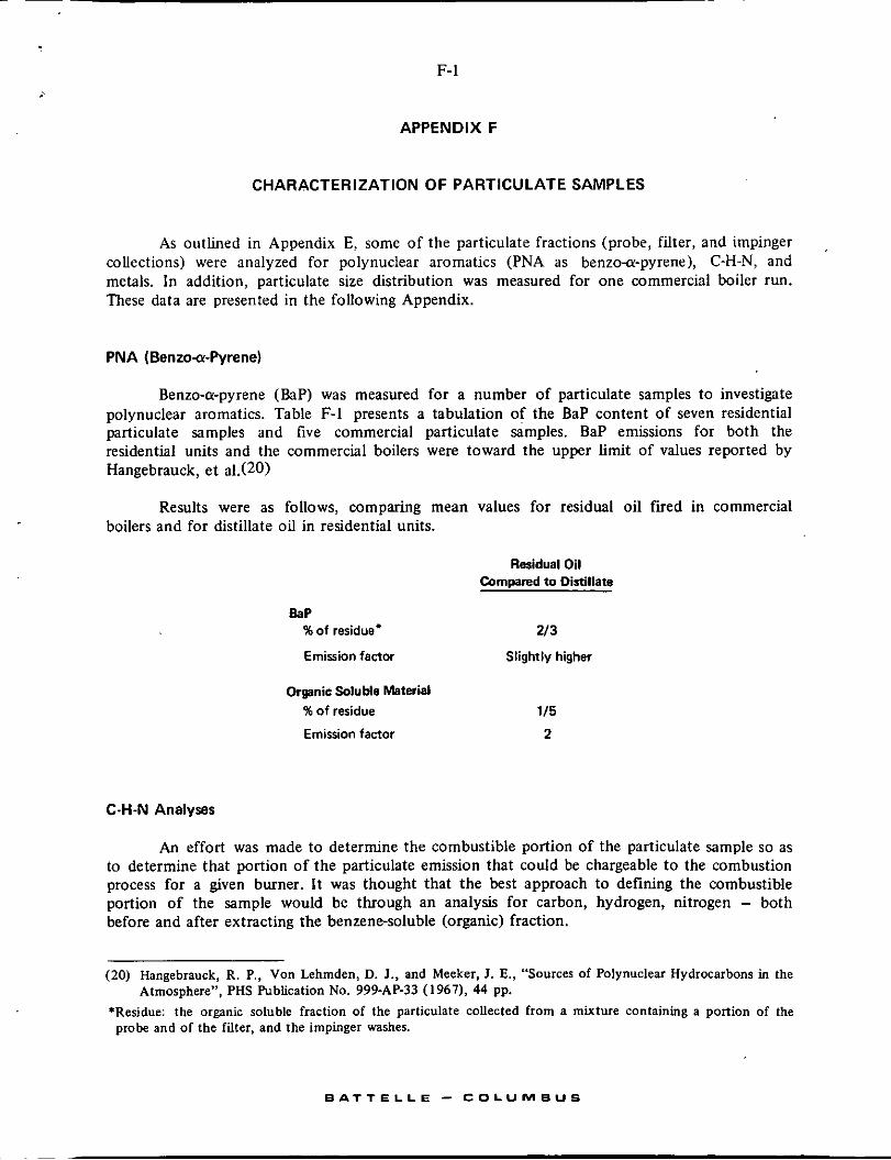
F- 1

APPENDIX F

CHARACTERIZATION OF PARTICULATE SAMPLES

As outlined in Appendix E, some of the particulate fractions (probe, filter, and impinger collections) were analyzed for polynuclear aromatics (PNA as benzoa-pyrene), C-H-N, and metals. In addition, particulate size distribution was measured for one commercial boiler run. These data are presented in the following Appendix.

PNA (Benzoa-F‘yrene)

Benzo-a-pyrene (BaP) was measured for a number of particulate samples to investigate polynuclear aromatics. Table F-1 presents a tabulation of the BaP content of seven residential particulate samples and five commercial particulate samples. BaP emissions for both the residential units and the commercial boilers were toward the upper limit of values reported by Hangebrauck, e t a1.(20)

Results were as follows, comparing mean values for residual oil fired in commercial boilers and for distillate oil in residential units.

Raridual Oil Compared to Disiillau,

BaP %of residue’

Emission factor

Organic Soluble Material %of residue

Emission factor

21 3

Slightly higher

115 2

C-H-N Analyses

An effort was made to determine the combustible portion of the particulate sample so as to determine that portion of the particulate emission that could be chargeable to the combustion process for a given burner. It was thought that the best approach to defining the combustible portion of the sample would be through an analysis for carbon, hydrogen, nitrogen - both before and after extracting the benzene-soluble (organic) fraction.

(20) Hangebrauck, R. P., Von Lehmden, D. I., and Meeker, J. E., “Sources of Polynuclear Hydrocarbons in the

‘Residue: the organic soluble fraction of the particulate collected from a mixture containing a portion of the Atmosphere”, PHS Publication No. 999-AP-33 (19671, 44 pp.

probe and of the filter, and the impinger washes.


F-2

Table F-1. Benzo-a-Pyrene Analyses

Unit and Fuel pg BaP(0) mg Residue Ib Residue Ib BaP Cundition Grade mg Residue mg Particulate 1000 gal Fuel 1000 gal Fuel

R as i d mti a l

3A

8A

8T

9A

9T

14A

1 4T

Mean -

Commercial

c1001 L

Cl002 H

C1002 H-S3

C1005 H

C1008 H

Mean

2 0.23

2 0.26

2 0.43

2 0.31

2 0.43

2 0.76

0.34 2

0.39

-

0.153

0.233

0.244

0.180

0.074

0.073

0.236

0.170 -

0.73

0.62

0.80

0.60

0.53

0.48 0.91

0.67 -

Range reported by Hangebrauck, et a((’’)

6 0.13

5 0.29

6 0.30

4 0.29

0.31 5

0.26 -

Range reporte

0.064 1.68

0.037 1.40

0.020 1.52

0.020 0.71

0.77 0.043

0.037 1.22 - -

I Hangebrauck, et al (22)

o.om17

0.00016

0.00034

0.00019

0.00024

0.00037

0.00031

0.00025

0.00001

{ 0.&31

-

0 . m 2 0.00041

0 . W 6

0.00021

0.00024

0.00031

0.00001 to

O.WO31

-

~~

(a) Mean precision f 12 percent.

F-4

Tables F-2 and F-3 present C-H-N analyses samples from residential units and commercial boilers, respectively. Table F-4 gives the C-H-N analyses of the sample portion remaining after benzene extraction for a few selected samples. The scatter in these few data is so large that it is impossible to draw meaningful conclusions from them.

I f the assumption is made that the carbon and hydrogen in the samples are solely carbon and organic compounds, the data could be used to calculate a “combustible fraction” of the particulate. However, the spread in these data is large, and 3 more detailed analysis on a larger number of samples is needed to quantify the combustible fraction of the particulate.

Table F-4. C-H-N Analyses of Particulate From Residential Units After Benzene Extractionlal

Analyses of lnroluble Residue Portion

Unit and Extraction, percent percent Condition C H N C H

Remaining After Benzene Extracted,

8A 16.1 0.60 <0.27 11.2 - 9A 53.6 0.58 <0.24 5.2 0.00

9T 4.4 0.87 <0.29 2.4 0.22

14A 77.6 0.69 <0.07 17.7 0.11

1 4T 17.7 0.39 <0.53 10.4 1.34

(0) Percentage based on filter sample weight before extraction.

Because the C-H-N data only accounted for a portion of the sample, a total sulfur analysis was performed on several samples to determine if significant portions of the samples were sulfur. Table F-5 shows that, for the samples analyzed, about 5 percent of the probe wash and 15 to YY percent of the impinger wash was sulfur. Results of these analyses indicate that more complete analyses (or a t least sulfur analyses) should be performed on further samples.

Table F-5. Sulfur Content of Several Particulate Samples

Boiler and Condition Robe Wash lmpinger Wash

Total Sulfur Content, percent

C1001H 3.7 99

C1002H-S1 7.1 15

C1002H-S2 4.4 26

C1007H 5.8 96


F-5

Trace Metals

It is recognized that numerous trace metals are introduced into the atmosphere as a result of the combustion of oil and coal. A number of the particulate samples collected from residential and from commercial units were analyzed by optical emission spectroscopy for trace metals. These dJta are semiquantitative and are presented in Tables F-6 and F-7.

Tables F-8 and F-9 show emission factors for the metals for these samples. It is cf interest to note that a larger number of trace metals are observed in the probe and impinger fractions. The levels of the trace metals are sufficiently low that they may only reflect trace impurities in the probe and impinger glass apparatus. It will be noted that the principal trace metals observed in the filter samples collected from residential units are iron, magnesium, lead, and aluminum. In the case of the commercial units, vanadium, nickel, aluminum, and calcium are highest, reflecting the fact that the three samples were obtained when fuing No. 4, No. 5, and No. 6 residual oils.

Particle-Size Distribution

A particle-size distribution was obtained on the particulate in one commercial boiler, C1002, Run H-S3, firing No. 6 fuel oil with a No. 5 Bacharach smoke number. The results of two cascade impactor measurements were averaged and the data are presented in Figure F-I. The particle-size range is based on an estimated specific gravity of 3.86 for the particles. On this basis, 25 percent (by weight) of the particles were smaller than 0.21 micron and 80 percent were smaller than 7.4 microns with a mass mean particle size of about 1.2 microns. (Additional investigation of particle size is planned in Phase I1 of this program.)

B A T T E L L E - E O L U M ~ U S

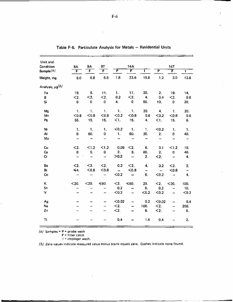
F-6

Table F-6. Particulate Analysis for Metals - Residential Units

Unit and Condition sample fa)

Weight, mg 6.0 6.8 5.5 1.8 23.6 15.6 1.2 3.0 13.6

Analysis, pdb)

8A 9A 9T 14A 14T --- F F F P F I P F I - - - - - - - - -

Fe 19. 5. 11. 1 . 11. 20. 2. 19. 14. B <2. <2. <2. 0.2 <2. 4. 0.4 <2. 0.6 Si 0 0 0 4. 0 50. 10. 0 20.

Mg 1. 1. 1 . 1. 1. 20. 4. 1 . 20. Mn <0.8 <0.8 <0.8 <0.2 <0.8 0.6 <0.2 <OB 0.6 Pb 55. 15. 15. <l. 15. 4. <l. 15. 6.

Ni AI Mo

1. 1. 1. (0.2 1. 1. <0.2 1. 1. 0 60. 0 1. 60. 30. 2. 0 40.

- - - - - - - - -

cu <2. <1.2 <1.2 0.06 <2. 6. 0.1 <1.2 10. ca 0 5. 0 2. 3. 60. 2. 0 40.

- >0.2 - 2. <2. - 4. cr

Ba <2. <2. <2. 0.2 <2. 4. 0.2 <2. 2. Bi G4. < O B <0.8 - <0.8 - - <0.8 -

- <0.2 - 6. <0.2 - 4. co

K <20. <20. G60. <2. -30. 20. <2. <20. 100. 0.2 - 6. 0.2 - 10. Sn

V - - - <0.2 - <0.2 <0.2 - <0.2

- -

- -

- - -

Ag Na Zn

- - - <0.02 - 0.2 <0.02 - 0.4 - - - <2. - 100. <2. - 200.

- <2. - 6. <2. - 6. - -

0.4 - 1.6 0.4 - 2 - - - Ti

(a) Samples = P = probe wash F = filter catch I = impinger wash.

(b) Zero values indicate measured value minus blank equals zero. Dashes indicate none found,

' J

F-7

Table F-7. Particulate Analysis for Metals - Commercial Boilers(')

Unit and Condition c1001 L C1002H C1007L Sample(") Weight, mg 21. 52.1 85.8 21.6 28.8 115. 6.2 25.8 31.

Analysis. &fb)

P F I P F I P F I - - - - - - - - -

Fe 10. 16. 20. 40. 16. 10. 10. 4. 10. 8 1. <2. 10. 20. <2. 10. 14. <2. 0.4 Si 40. 0 60. 100. 0 60. EO. 0 30.

Mg 20. 14. 60. 60. 2. 10. 20. 14. 6. Mn 0.4 <0.8 2. 1. <0.8 1. 0.4 <0.8 0.2 Pb 6. 0 6. 4. 0 4. 2. 0 1.

Ni 4. 396. 100. 80. 196. 1. 10. 196. 0.4 AI 60. 480. 600. 60. 680. 10. 60. 480. 6. MO <0.2 1.2-2. 0.2 0.6 < O B <0.2 <0.2 <0.8 <0.2

cu 8. 0 4. 4. 0 1. 2. 0 4. cd 400. 52. 300. 400. 52. 100. EO. 52. 30. Cr 0.4 0 20. 2. 0 1. 1. 0 0.2

Ba 2. <2. 30. 10. 2. 1. 30. <2. 2. Bi <0.2 0 <0.2 <0.2 0 <0.2 <0.2 0 <0.2 co 100. 2. 0.6 0.6 2. 4. <0.2 <2.0 <0.2

K 20. <20. 60. 40. <20. 10. 10. <20. 10. Sn 4. <0.8 4. 2. <0.8 <l. 2. < O B 2. V 10. 1600. 400. 200. 200. 1. 30. 800. 2.

Ag 1. - 4. 4. - <0.02 2. - 0.1 Na 200. 60. 400. 200. <60. 100. 20. 60. 40. Zn 4. <4. 6. 4. <4. <2. 4. <4. 2.

Ti 1. 15.2-16. 4. 2. 7.2-8. 1. 4. 3.2-4. 0.2 Zr <0.2 <20. <0.2 <0.2 16.-20. <0.2 <0.2 16:20. <0.2

(a) Sampler: P = probe wash F = filter catch I = impinger wash.

( b ) Zero values indicate measured value minus blank equals zero. Dashes indicate none found.

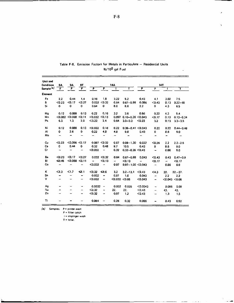
Table F-8. Emission Factors for Metals in Particulate - Residential Units lb1106 gal Fuel

Unit and Condition 8A 9A 9T 14A 14T S.mplsl"l F - F F - P F I T P F I T - - - - - - __ - - __ Element

Fe 8 Si

Mg M" Pb

Ni AI M O

C" Ca Cr

Ba Bi CO

K S" V

Ag N. Z"

Ti

2.2 0.44 1.4 <0.23 <0.17 <0.27

0 0 0

0.12 0.088 0.13 <0.092 <0.068 <0.11

6.3 1.3 2.0

0.12 0.088 0.13 0 2.6 0 - -

<0.23 <0.096 <0.17 0 0.44 0 - - -

<0.23 <0.17 <0.27 a . 4 5 <o.oEa <0.11 - - -

a . 3 <1.7 c8.1 - - - - - -

0.16 1.8 0.032 < O X 0.64 0

0.22 0.16 <0.032 <0.13 <0.22 2.4

<0.032 0.16 0.22 4.8' - -

0.097 <0.32 0.32 0.48

<0.032 -

0.032 <OX' - <0.13

<0.032 - <0.32 C9.6

0.032 - <0.032 -

0.W32 - <0.32 - <0.32 -

0.064 -

3.22 5.2 0.43 0.64 0.67-0.99 0.086 8.0 8.6 2.2

32 3.6 0.86 0.097 0.10-0.26 <0.043 0.64 3.0-3.2 <012

0.22 0.38-0.41 <0.043 4.8 9.8 0.43 - - -

0.97 0.98-1.30 0.022 9.7 10.5 0.43 0.32 0.32-0.35 <0.43

0.64 0.67-0.99 0.043 - <0.13 - 0.97 0.97-1.00 <0.043

3.2 3.2-13.1 <0.43 0.97 1.0 0.043

<0.032 <0.06 <0.043

0.032 0.035 <0.0043 22. 22. <0.43 0.97 1.2 <0.43

0.26 0.32 0.086

4.1 <0.43

0

0.22 <0.17

3.2

0.22 0 -

<026 0 -

<0.43 <0.17 -

<4.3 - - - - - -

3.02 7.5 0.13 0.22-65 4.3 6.5

4.3 5.4 0.13 0.13-0.34 0.13 3.3-3.5

0.22 0.44-0.48 8.6 9.0 - -

2.2 2.2-2.5 8.6 9.0 0.86 9.0

0.43 0.47-0.9 - <0.17 0.86 0.9

22. 22.-27 2.2 2.2

<0.043 <0.08

0.086 0.09

1.3 1.5

0.43 0.62

43. 43.

lo) Samples: P - probe Wash F - filter Catch I - impinper wash

T - total.

~

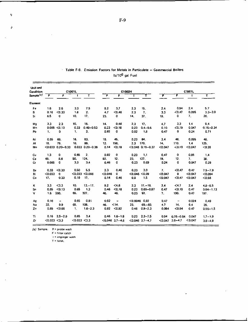
t

F-9

Table F-9. Emission Factors for Metals in Particulate - Commercial Boilers lb/1o6 gal F U ~ I

Unit and Condition C l O O l L ClWZH C1007L

F I T P F I T P F I T

Element

Fe 8 Si

Mg M" Pb

Ni AI MO

C" Ca C I

Ea Bi c o

K Sn V

AO Na Zn

Ti Z I

--- 1.6 2.6 3.3 7.5 0.16 <0.33 1.6 2. 6.5 0 10. 17.

9.2 3.7 2.3 15. 4.7 <0.46 2.3 7.

23. 0 14. 37.

2.4 0.94 2.4 3.3 40.47 0.W5

19. 0 7.

3.3 2.3 10. 16. 14. 0.46 2.3 17. 4.7 3.3 1.4 0.065<0.13 0.33 0.40-0.53 0.23 <0.18 0.23 0.4-0.6 0.10 10.19 0.047 1. 0 1. 2.

0.66 66. 16. 83. 10. 79. 10. 99. <0.033 0.20-0.33 0.033 0.20-0.38

1.3 0 0.65 2. 65. 8.6 50. 124. 0.065 0 3.3 3.4

0.33 <0.33 0.50 5.5 <0.033 0 <0.033 <0.066 17. 0.33 0.10 17.

3.3 <3.3 10. 13.-17. 0.65 <0.13 0.65 1.3 1.6 2W. 65. 327.

0.16 - 0.65 0.81

0.65 <0.66 1. 1.6-2.3

0.16 2.5-2.6 0.65 3.4 <0.033 <3.3 <0.033 <3.3

33. 9.9 65. loa.

0.92 0 0.92 1.8

19. 45. 0.23 64. 12. 156. 2.3 170. 0.14 <O.l8 <0.046 0.19-0.37

0.92 0 0.23 1.1

0.46 0 0.23 0.69 92. 12. 23. 127.

2.3 0.46 0.23 3.0 <0.046 0 <OB46 <O.W

0.14 0.46 0.9 1.5

9.2 <4.6 2.3 11.-16. 0.46 <0.18 0.23 0.69-0.87

46. 46. 0.23 92

0.92 - <O.W46 0.92 46. <14. 23. 69.43. 0.92 <0.92 0.46 0.9-2.3

0.46 1.6-1.8 0.23 2.3-2.5 <OD46 3.7-4.6 < O M 6 3.7-4.7

0.47 0 0.24

2.4 46. 0.095 14. 110. 1.4

<0.047 10.19 <OB47

0.47 0 0.95

0.24 0 0.047 19. 12. 7.

7. 10.47 0.47 <O.047 0 <O.M7 <OM7 <0.47 <0.047

2.4 <4.7 2.4 0.47 <0.19 0.47 7. 190. 0.47

0.47 - 0.024 4.7 14. 9.4 0.094 ~ 0 . 9 4 0.47

0.94 0.75-0.94 0.047 < O M 7 3.8-4.7 <0.047

5.7 3.3-3.9

26.

9.4

0.71 0.15-0.34

48. 125. <0.28

1.4

0.29

7.5-7.9 <0.094 <OS6

4.8-9.5 0.94- 1.13

38.

197.

0.49 28. 0.56- 1.5

1.7-1.9 3.8-4.8

(0) Sample: P = probe wash F = fi lter Catch I = impinger wash

T = total.

9

9

9

9

8

7

6

5

4'

31

21

I 1

O.!

0.0 0.2

F-IO

u-u 0.3 0.4 0.5 0.6 0.8 I 2 3 4 5 6 7 8 9

Particle size,p

7.0 3.5 I .8 0.88 0.44 0.2

Particles less than this size, weight percent

81 68 57 45 35 20

Figure F-1. Particle-Size Distribution - Boiler C1002, Run H-S3

. G- 1

APPENDIX G

DETAILS OF EMISSION-FACTOR CALCULATIONS AND CONVERSION FACTORS

Emission factors are commonly defined in terms of the weight of pollutant emissions per unit of fuel input - either weight, volume, or Btu heating value of the fuel. For purposes of this report, emission factors for oil-fired equipment are expressed in terms of pounds pollutant per thousand gallons of fuel oil input as this is the basis of the published emission factors compiled by Duprey and is convenient in developing emission inventories.

Calculation of the emission factors requires data on ( I ) the concentration .of the pollutant (e.g., ppm for gaseous pollutants or grains per cubic foot of flue gas for particulate) and (2) the rate of generation of flue gas. This latter quantity may be determined by one of several approaches, depending on data available. Four alternate approaches are feasible, requiring the following information:

1. Measurement of flue-gas flow rate, plus flue-gas analysis (used where

2. Measurement of flue-gas flow rate, plus fuel firing rate

3. Fuel firing rate, plus flue-gas analysis (the most frequently used technique)

4. Fuel composition (C-H), plus flue-gas analysis.

fuel composition and firing rate are unknown)

Of these approaches, the fourth was chosen as being consistently the most accurate for the conditions of the field investigation. This approach is outlined in the following section for distillate fuel oil and residual fuel oil respectively.

Emission Factor Calculations for Distillate Fuel Oil

The combustion equation, assuming negligible CO and HC, is

CHE + ( 1 .O + 0.25E + X) 0 2 + [( 1 .O + 0.25E + X)3.77] N2

= C02 + 0.5E H 2 0 + X 02 + [(1.0 + 0.25E + X)3.77]N2

, where E = ratio of hydrogen atoms to carbon atoms in the fuel,

12.01 (% H in fuel) 1.008 (% C in fuel) E =

X = ratio of percent 0 2 to percent C 0 2 in flue gas.


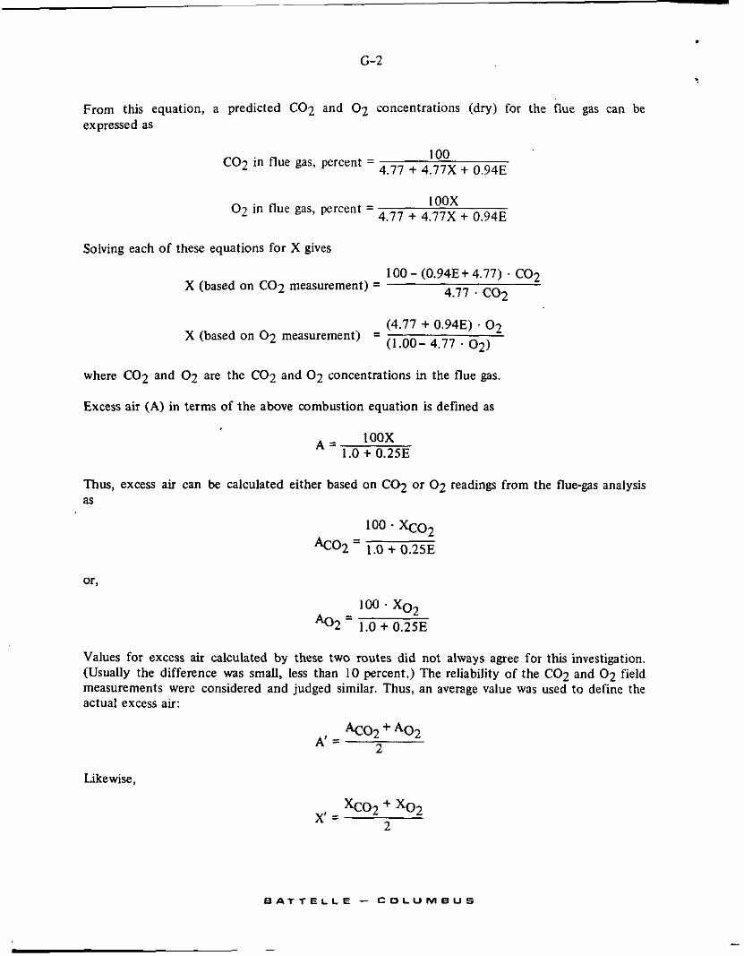
G 2

From this equation, a predicted CO2 and 0 2 concentrations (dry) for the flue gas can be expressed as

100 4.77 t 4.77X + 0.94E CO2 in flue gas, percent =

I oox 4.77 -t 4.77X t 0.94E 0 2 in flue gas, percent =

Solving each of these equations for X gives

100 - (0.94E+ 4.77) . C02 4.77 . c 0 2 X (based on CO2 measurement) =

(4.77 + 0.94E) . 0 2 (1.00- 4.77 ' 0 2 )

X (based on 0 2 measurement) =

where C02 and 0 2 are the C02 and 0 2 concentrations in the flue gas.

Excess air (A) in terms of the above combustion equation is defined as

1 oox 1.0 + 0.25E A =

Thus, excess air can be calculated either based on C02 or 0 2 readings from the flue-gas analysis as

or, 100 ' xo2

A'2 = 1.0 + 0.25E

Values for excess air calculated by these two routes did not always agree for this investigation. (Usually the difference was small, less than IO percent.) The reliability of the CO2 and 0 2 field measurements were considered and judged similar. Thus, an average value was used to define the actual excess air:

4 0 2 t A 0 2 A' E

2

Likewise,


i

G 3 c

The weight (W) of dry flue gas generated in pounds per pound of fuel fired at this average excess air is

1.0 . 44.01) + (X' . 32.0) +{[(l.O + 0.25E + X')3.77128.02) (12.01) + (E . 1.008) W = I

The volume (V) of dry flue gas generated (cubic feet at 7 0 F per pound of fuel tired) is

W v=- 0.075

Gaseous emission factors, EF, can now be calculated as

V . PPM . MW . FD 386 . 1000 EFa (Ib pollutant/ IO00 gal fuel) =

where PPM = concentration of pollutant in flue gas (dry)

MW = molecular weight of pollutant

FD = fuel density in Ib/gal.

Particulate emission factors, EF', can be calculated as follows:

V . GL . FD EF', (Ib pollutant/l000 gal fuel) =

GL = grain loading measured in sampled gas in grains per standard where cubic foot (dry at 70 F).

Conversion Factors for No. 2 Fuel Oil

Emission factors in lb/1000 gal may be converted to other units as follows:

Gaseous Emissions

EFb (kg pollutant/1000 liter fuel) = EFa . 0.1198

EFc (Ib pollutant/l000 Ib fuel) EFa = - FD

which, for a typical No. 2 fuel oil of 33 degrees API gravity, becomes

EFC = E F a . 0.139

EFd (g pollutantlkg fuel) = EFc = EFa . 0.139 - EF, . 103 EFe (Ib pollutant/l06 Btu) -

Heating value of fuel (Btu/gal)


which, for No. 2 fuel of API gravity 33, becomes

EFe = EFa . 0.00715.

It is sometimes convenient to express emissions in ppm at some standard condition, for example:

PPM . V EFf (ppm pollutant at 12% CO2 dry) = "I 2% c 0 2

or

which, for No. 2 fuel of MI gravity 33, becomes

EFa , 218 E F f = MW .

Particu/ate Emissions. Similarly for particulate, EFb', EF,', EFd', and EF,' follow from EF,'. An additional emission factor is sometimes used for particulate emissions as follows:

EFf' (Ib pollutant/106 scf flue gas at 12 percent C02, dry)

- GL . 1000 V - 7 V12% c 0 2

or

EF,' . 1000 - - FD . "1 2% c02

which, for No. 2 fuel oil of APl gravity 33, becomes

EFf' = EF,' . 0.565 . Emission Factor Calculations for Residual Fuels .B'

A similar technique to that described above was used to calculate emission factors for residual fuels. However, these calculations included the sulfur and nitrogen in the fuel, assuming all of the S and N from the fuel appeared as SO2 and NO in the flue gas, respectively. The combustion equation became

CHESFNG + ( 1 .O + 0.2SE + F + 0.5G + X)02

+[(1.0 + 0.2SE + F + 0.5G + X)3.771N2 = C 0 2 + 0.SE-H20

+ F.SO2 + G.NO + X.02

+ I ( l . O + 0.25E + F + 0.5G + X)3.77lN2


. G-5

where

F = ratio of sulfur atoms to carbon atoms in the fuel

- 12.01 . (%S in fuel) 32.06 . (%C in fuel)

-

and

G = ratio of nitrogen atoms to carbon atoms in the fuel

- 12.01 . (%N in fuel) - 14.008 . (%C in fuel)

It follows that

W = (1.0.44.0 I)+(F~64.06)+(C~30.01 )+(X'.32.0)+{[( 1.0+0.25E+F+O.SG+X')3.77] 28.02) (1 2.01 )+(E~l.008)+(F~32.06)+(G~14.02)

where the expression for X' includes SO2 and NO, terms.

However, V, EF,, and EF,' follow using the same relationships as for residential units.

Conversion Factors for No. 6 Oil

Conversion factors for obtaining emission factors in other units are similar to those used for residential units except where fuel properties are required. The conversion factors for a typical No. 6 fuel oil of 15 degrees API gravity are as follows.

Gaseous Emissions.

EFb = EFa . 0.1 198

EFc =. EFa . 0.124 EFd = EFa ' 0. I24

EFe = EFa 0.00661 lb/106 Btu.

kg/lOOO liter fuel

lb/1000 Ib fuzl

g/lOOO kg fuel

EFa . 200 EFf = -MW ppm @ 12% C02

Particulate Emissions. Similarly EFb,', EF,', EFd', and EF,' follow from EF,' and

EFf' = EF; . 0.520 lb/106 scf flue gas @ 12% C02

E A T T E L L E - E O L U M E U S

'. G-6

I

Summary of Conversion Multipliers

Table GI summarizes conversion multipliers for some of the common methods of expressing emission factors.

Table G-1. Multipliers to Convert Emission Factors From lbll000 gal to Other Units

Multiply Emissions Factor in lb/1000 gal Fuel (EFJ To Obtain Emission Factor

In These Units for NO. 2 Oil la) for No. 6 Oillb)

kg/1000 liter fuel 0.1198 0.1198

lb/lOOO Ib fuel 0.139 0.124

gmkg fuel 0.139 0.124

lb1106 8tu input 0.00715 0.00661

218 200 Gaseous pollutants(c), - ppm at 12% CO2 MW

Particulates, lb/106 scf flue gas a t 12% CO2 0.565 0.520

(a) /b) (c)

Typical No. 2 fuel oil having 33 API gravity. Typical No. 6 fuel oil having 15 API gravity, MW = molecular weight of pollutant.


R

1 u’

H- 1

APPENDIX H

REFERENCES

I . Duprey, R. L., “Compilation of Air Pollutant Emission Factors”, National Center for Air Pollution Control, U.S. Public Health Service Publication NO. 999-AP-42, 1968, p 7.

2. McGraw, M. J., and Duprey, R. L., “Compilation of Air Pollution Emission Factors”, Preliminary Document, Environmental Protection Agency, April, 1971, p IO.

3. Burroughs, L. C., “Air Pollution by Oilburners - Measurable but Insignificant”, Fuel Oil and Oil Heat, June, 1963, pp 43-46+.

4. Howekamp, D. P., and Hooper, M. H., “Effects of Combustion-Improving Devices on Air Pollutant Emissions from Residential Oil-Fired Furnaces”, APCA Paper No. 70-45, 1970, 33 PP.

5. Howekamp, D. P., “Flame Retention - Effects on Air Pollution”, Presented at 9th Annual Convention, NOFI, Atlantic City, New Jersey, June 9-11, 1970, 10 pp.

6. Bunyard, F. L., and Copeland, J. O., “Soiling Characteristics and Performance of Domestic and Commercial Oil Burning Units”, NAPCA, January 28, 1968.

7. Scott Research Laboratories, Inc., reports on NCAPC Contracts No. PH 27-00154 and PH 22-68-125, 1968.

8. Private communication: to D. W. Lmklin, Battelle-Columbus, from Norton Saude, Honeywell, Inc. (February 26, 1971).

9. Private communication: t o D. W. Locklin, Battelle-Columbus, from W. F. Hergrueter, Mobil Oil Corporation (April 22, 1971).

10. Wasser, J. H., Hangebrauck, R. P., and Schwartz, A. J., “Effects of Air-Fuel Stoichiometry on Air Pollutant Emissions from an Oil-Fired Test Furnace”, Journal of Air Pollution Control Association, Vol 18, No. 5 , May, 1968, pp 332-337.

1 1. “Specifications for Incinerator Testing at Federal Facilities”, U.S. Department of Health, Education, and Welfare, Public Health Service, Bureau of Disease Prevention and Environ- mental Control, National Center for Air Pollution Control, October, 1967, 34 pp.

12. “Standards of Performance for New Stationary Sources”, Federal Register, Vol. 36, No, 139, Part 11, pp 15704-15722, August 17, 1971.


1

H-2 I

13. NAPCA RFP No. CPA 70-Neg. 218, Scope of Work, 1971, p 1 .

14. Hunt, R. A., Jr., and Biller, R. E., Conference Paper CP61-6, Proceedings: API Research Conference on Distillate Fuel Combustion, API Publication 1541, 1961.

15. Paterson, R. E., “Nitrogen Oxides in Combustion Gases”, Chevron Research Corporation, Internal Report, File 084.0, April I I , 1961.

16. Martin, G. B., Pershing, D. W., and Berkau, E. E., “Kinetics of the Conversion of Various Fuel Nitrogen Compounds to Nitrogen Oxides in Oil Fired Furnaces”, AIChE Paper No. 37f, 70th National Meeting, Atlantic City, August 29-September 1, 1971.

17. Bartok, W., Engleman, V. S., Goldstein, R., and Valle, E. D., “Basic Kinetic Studies and Modeling of Nitric Oxide Formation in Combustion Processes”, AIChE Paper 37d, 70th National Meeting, Atlantic City, August 29-September I , 1971.

18. Shelton, E. M., “Burner Fuel Oils”, 1971, U S . Department of Interior, Bureau of Mines, Petroleum Products Survey No. 71, August, 1971, p 19.

19. Pilcher, J . M., Mitchell, R. I. , and Thomas, R. E., “The Cascade Impactor for Particle-Size Analysis of Aerosols”, Presented to Chemical Specialists Manufacturers Assoc., Inc., New York City, December 6 and 7, 1955.

20. Hangebrauck, R. P., Von Lehmden, D. J., and Meeker, J. E., “Sources of Polynuclear Hydrocarbons in the Atmosphere”, PHS Publication No. 999-AP-33, 1967, 44 pp.

’


Title: A of Space 4099 Levy, A., et ai.

Documents

Transcript of Title: A of Space 4099 Levy, A., et ai.