Tissue Fluorescence Spectroscopy

Lecture 16

Outline• Steady-state fluorescence

– Instrumentation and Data Analysis Methods• Statistical methods: Principal components analysis• Empirical methods: Ratio imaging• Modeling: Quantitative extraction of biochemical info

– Fluorescence in disease diagnostics– Fluorescence in disease therapeutics

Fluorescence spectra provide a rich source of information on

tissue state

-1

-0.5

0

0.5

1

1.5

350 400 450 500 550 600300

350

400

450

Emission (nm)

Exc

itatio

n (

nm)

NADH

FAD

Collagen

Trp

Protein expression

Structural integrity

Metabolic activity

Courtesy of Nimmi Ramanujam, University of Wisconsin, Madison

Development of cancer involves a series of changes some of which can be probed by fluorescence

•protein expression (Trp)•metabolic activity (NADH/FAD)•nuclear morphology

•organization•structural integrity (collagen)•angiogenesis

Instrumentation for clinical tissue fluorescence measurements can be very simple, compact and

relatively cheap

Courtesy of Urs Utzinger, University of Arizona

Light Source

CCD

Control

ImagingSpectrograph

Optical fiber probe

Consistent autofluorescence differences have been detected between normal, pre-

cancerous and cancerous spectra

300 400 500 600 700

0.0

0.2

0.4

0.6

0.8

1.0

Non-dysplastic Barrett’s esophagus Low-grade dysplasiaHigh-grade dysplasia

Wavelength (nm)

Nor

mal

ized

fluo

res c

enc e

inte

nsi ty

Promising studies in•GI tract•Cervix•Lung•Oral cavity•Breast•Artery•Bladder

Methods of data analysis

• Main goal for fluorescence diagnostics: Identify fluorescence features that can be used to identify/classify tissue as normal or diseased.

• Main approaches– Statistical– Empirical – Model Based

Data analysis: Empirical and statistical algorithms

Data pre-processing

Normalization

Data reductionand

Feature extraction

Principal ComponentAnalysis Ratio methods

Classification

Detection of cervical pre-cancerous lesions using

fluorescence spectroscopy: Principal components analysis

Rebecca Richards Kortum group UT Austin

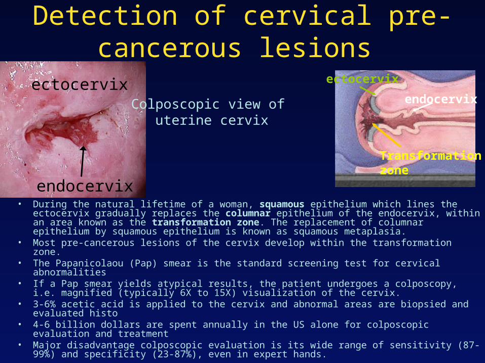
Detection of cervical pre-cancerous lesions

• During the natural lifetime of a woman, squamous epithelium which lines the ectocervix gradually replaces the columnar epithelium of the endocervix, within an area known as the transformation zone. The replacement of columnar epithelium by squamous epithelium is known as squamous metaplasia.

• Most pre-cancerous lesions of the cervix develop within the transformation zone.• The Papanicolaou (Pap) smear is the standard screening test for cervical abnormalities• If a Pap smear yields atypical results, the patient undergoes a colposcopy, i.e. magnified

(typically 6X to 15X) visualization of the cervix.• 3-6% acetic acid is applied to the cervix and abnormal areas are biopsied and evaluated

histo• 4-6 billion dollars are spent annually in the US alone for colposcopic evaluation and treatment• Major disadvantage colposcopic evaluation is its wide range of sensitivity (87-99%) and

specificity (23-87%), even in expert hands.

endocervix

ectocervix

Transformation zone

Colposcopic view of uterine cervix

ectocervix

endocervix

Major tissue histopathological classifications

• Normal squamous epithelium• Squamous metaplasia• Low-grade squamous intraepithelial lesion• High-grade squamous intraepithelial lesion• Carcinoma

Instrumentation

Nitrogen Pumped Dye

Laser

Nitrogen Pumped Dye

Laser

337 nm

380 nm

460 nm

PolychromatorIntensifiedDiode Array

Gate Pulser Controller Computer

collection fibers

excitation fibers

excitation fiberscollection fibers quartz

shield

Spectral Resolution: 10 nm

30 Hz rep rate5 ns pulse duration

probe

PRE-PROCESSING

Normalized Spectra at Three Excitation Wavelengths

Normalized, Mean-scaled Spectra at Three Excitation Wavelengths

DIMENSION REDUCTION: PRINCIPAL COMPONENT ANALYSIS 

CLASSIFICATION: LOGISTIC DISCRIMINATION 

Posterior Probability of being NS or SIL

Posterior Probability of being LG or HG

Posterior Probability of being NC or SIL

Posterior Probability of being SIL or NON SIL

Posterior Probability of being HG SIL or NON HG SIL

DEVELOPMENT OF COMPOSITE ALGORITHMS

Constituent Algorithm 1 Constituent Algorithm 3 Constituent Algorithm 2

(1,2) (1,2,3)

SELECTION OF DIAGNOSTIC PRINCIPAL COMPONENTS: T-TEST 

Composite Screening Algorithm Composite Diagnostic Algorithm

337 nm Excitation 380 nm Excitation 460 nm Excitation

0

0.1

0.2

0.3

0.4

0.5

350 400 450 500 550 600 650

Wavelength (nm)

Flu

ores

cenc

e In

tens

ity

NS

NC

LGHG

0

0.1

0.2

0.3

400 450 500 550 600 650

Wavelength (nm)

Flu

ores

cenc

e In

tens

ity

NS

NCHG

LG

0

0.1

0.2

0.3

460 510 560 610 660

Wavelength (nm)

Fluo

resc

ence

Inte

nsity

NS

NCLG

 

Courtesy of N. Ramanujam; Photochem. Photobiol. 64: 720-735, 1996

00.10.20.30.40.5

350 450 550 650

Wavelength (nm)F

luo

resc

ence

In

ten

sity

(c

.u.)

00.20.40.60.8

11.2

350 450 550 650

Wavelength (nm)

No

rmali

zed

Flu

ore

scen

ce I

nte

nsit

y

(c.u

.)

-0.4-0.2

00.20.4

350 450 550 650

Wavelength (nm)

Nor

mal

ized

, m

ean-

scal

ed

Flu

ores

cenc

e

Data

Pre-ProcessingStep 1

Pre-ProcessingStep 2

Normal squamousLow-gradeHigh-gradeNormal columnar

Principal Component Analysis

Spectrum= wi*Bi

w=component weightB=component loading describing data variance

00.20.40.60.8

11.2

350 450 550 650

Wavelength (nm)

No

rmali

zed

Flu

ore

scen

ce I

nte

nsi

ty

(c.u

.)

spectra Component loadings

Dimension reduction: Principal Component Analysis

00.20.40.60.8

11.2

350 450 550 650

Wavelength (nm)

No

rmali

zed

Flu

ore

scen

ce I

nte

nsit

y

(c.u

.)

0

0.2

0.4

0.6

0.8

1

1.2

400 500 600

Wavelength (nm)

No

rm

alized

F

lu

orescen

ce

In

ten

sity

(c.u

.)

0

0.2

0.4

0.6

0.8

1

460 560 660

Wavelength (nm)

Norm

ali

zed F

luo

rescence

Inte

nsit

y (

c.u

.)

Component loadingsspectra337 nm

380 nm

460 nm

PCA Step 2: Calculate probability of belonging to category based on component weights and classify

Sample Number

Post

erio

r Pr

obab

ilit

y of

SIL

0

0.25

0.5

0.75

1

0 50 100 150 200

Low Grade SIL

High Grade SIL

Normal Squamous

Sample Number

Post

erio

r Pr

obab

ilit

y of

SIL

0

0.25

0.5

0.75

1

80 100 120 140 160 180 200

Low Grade SIL

High Grade SIL

Normal Columnar

▲Low-grade SIL

●High-grade SIL

□Normal squamous

▲Low-grade SIL

●High-grade SIL

□Normal columnar□ Non-dysplastic Barrett’s esophagus

X Dysplatic Barrett’s esophagus

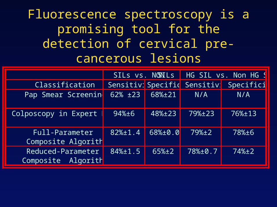
Fluorescence spectroscopy is a promising tool for the detection of cervical pre-

cancerous lesions

SILs vs. NON SILs HG SIL vs. Non HG SILClassification Sensitivity Specificity Sensitivity Specificity

Pap Smear Screening 62% ±23 68%±21 N/A N/A

Colposcopy in Expert Hands 94%±6 48%±23 79%±23 76%±13

Full-Parameter Composite Algorithm

82%±1.4 68%±0.0 79%±2 78%±6

Reduced-ParameterComposite Algorithm

84%±1.5 65%±2 78%±0.7 74%±2

Spectroscopic analysis using PCA

• Uses full spectrum information to optimize sensitivity and specificity

• Relatively easy to implement (automated software)

• Provides no intuition with regards to the origin of spectral differences

Spectroscopic imaging: fluorescence ratio methods for

detection of lung neoplasia

B. Palcic et al, Chest 99:742-3, 1991

LIFE schematic

B. Palcic et al, Chest 99:742-3, 1991

Detection of lung carcinoma in situ using the LIFE imaging

system

Courtesy of Xillix Technologies (www.xillix.com)

White light bronchoscopy Autofluorescence ratioimage

Carcinoma in situ

Autofluorescence enhances ability to localize small neoplastic lesions

Severe dysplasia/Worse Intraepithelial Neoplasia WLB WLB+LIFE WLB WLB+LIFE

Sensitivity 0.25 0.67 0.09 0.56

Positive predictive value

0.39 0.33 0.14 0.23

Negative predictive value

0.83 0.89 0.84 0.89

False positive rate 0.10 0.34 0.10 0.34

Relative sensitivity 2.71 6.3

S Lam et al. Chest 113: 696-702, 1998

Test DefinitionsHas disease Does not have

disease

Tests positive (A)

True positive

(B)

False positive

(A+B)

Total # who test positive

Tests negative (C)

False negative

(D)

True negative

(C+D)

Total # who test negative

(A+C)

Total # who have disease

(B+D)

Total # who do not have disease

Sensitivity=A/(A+C)Specificity=D/(B+D)

Positive predictive value=A/(A+B)Negative predictive value=D/(C+D)

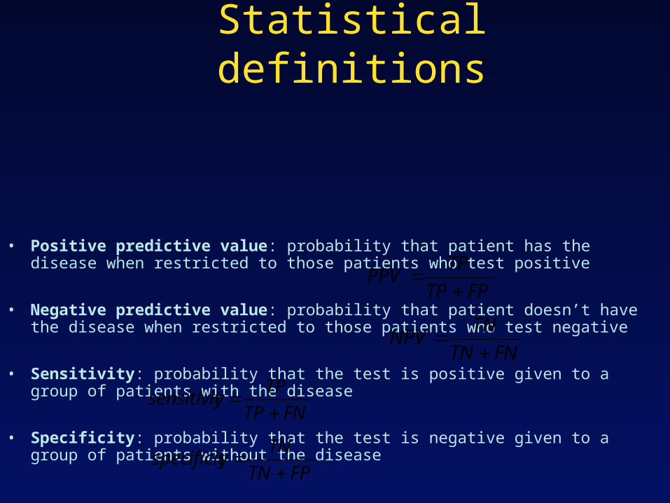
Statistical definitions

• Positive predictive value: probability that patient has the disease when restricted to those patients who test positive

• Negative predictive value: probability that patient doesn’t have the disease when restricted to those patients who test negative

• Sensitivity: probability that the test is positive given to a group of patients with the disease

• Specificity: probability that the test is negative given to a group of patients without the disease

FPTP

TPPPV

FNTN

TNNPV

FNTP

TPysensitivit

FPTN

TNyspecificit

Fluorescence imaging based on ratio methods

• Wide field of view (probably a huge advantage for most clinical settings)

• Eliminates effects of distance and angle of illumination

• Easy to implement• Provides no intuition with regards to

origins of spectral differences

What are the origins of the observed differences?

350 400 450 500 550 600 650 700 750

0.00

0.02

0.04

0.06

0.08

0.10

0.12

350 400 450 500 550 600 650 700 750

0.00

0.02

0.04

0.06

0.08

0.10

0.12

wavelength (nm)wavelength (nm)

Intr

insi

c fl

uo

resc

ence

Intr

insi

c fl

uo

resc

ence

337 nm excitation358 nm excitation381 nm excitation

397 nm excitation412 nm excitation425 nm excitation

Collagen NADH

Collagen and NADH spectra are sufficiently distinct only for some excitation

wavelengths

337 nm excitation 358 nm excitation

Tissue absorption and scattering may affect significantly tissue

fluorescence• scattering

– elastic scattering• multiple scattering

• absorption– Hemoglobin, beta carotene

• fluorescence

• single scattering

epithelium

Connective tissue

Is hemoglobin absorption a problem?

300 400 500 600 700 800

0.0

0.1

0.2

0.3

0.4

0.5

0.6

0.7

0.8

0.9

1.0

flu

ore

scen

ce

300 400 500 600 700 800

0.10

0.15

0.20

0.25

0.30

0.35

0.40

wavelength (nm)

refl

ecta

nce

337 nm excitation

wavelength (nm)

To get answer use

Monte Carlo simulations

Analytical Modeling