Time-Varying Demand for Lottery:

Speculation Ahead of Earnings Announcements*

Huijun Wang Jianfeng Yu Shen Zhao

March 2017

Abstract

Existing studies find that compared to non-lottery stocks, lottery-like stocks tend tobe overpriced and earn lower subsequent returns, probably due to investor preferencesfor lottery-like assets. We argue that investor preferences for holding speculative assetsare more pronounced ahead of firms’ earnings announcements, probably due to lowerinventory costs and immediate payoffs. We show that there is indeed stronger demandfor lottery-like stocks ahead of earnings announcements, leading to a price run-up forthese stocks. In sharp contrast to the standard underperformance of lottery-like stocks,we find that lottery-like stocks outperform non-lottery stocks by about 52 basis pointsin the 5-day window ahead of earnings announcements. However, this return spread isreversed by 75 basis points within five days after the announcements. Moreover, thisinverted-V shaped pattern on cumulative return spreads is more pronounced amongfirms with more retail order imbalance, with low institutional ownership, and in regionswith stronger gambling propensity.

JEL Classification: G02, G12, G14

Keywords: speculation, lottery, earnings announcements, skewness

*We thank Zhuo Chen and Zhiguo He for helpful comments and discussions. Wang: Lerner College

of Business and Economics, University of Delaware, 307A Purnell Hall, Newark, DE 19716. Email:

wangh@udel.edu, Phone: 302-831-7087. Yu: Carlson School of Management, University of Minnesota, 321

19th Avenue South, Suite 3-122, Minneapolis, MN 55455. Email: jianfeng@umn.edu, Phone: 612-625-5498,

Fax: 612-626-1335, and PBCSF, Tsinghua University, 43 Chengfu Road, Haidian District, Beijing, China.

Zhao: School of Management and Economics, Chinese University of Hong Kong (Shenzhen), 2001 Longxiang

Blvd, Longgang District, Shenzhen, China. Email: shenzhao@cuhk.edu.cn.

1 Introduction

Many studies find that investors exhibit a preference for speculative assets, and thus these

assets tend to be overvalued on average, leading to underperformance of these stocks relative

to non-speculative assets.1 In this paper, we argue that investors’ preferences for speculative

stocks are time-varying, and are especially strong ahead of firms’ earnings announcements.

Because the positions are held only for a short period of time, trading ahead of earnings

announcements reduces holding costs and inventory risk. Thus, speculative trading tends

to increase prior to earnings announcements. Since lottery-like assets are especially good

for speculation, the excess demand for these stocks should be notably higher especially

before earnings announcements. Moreover, due to the inventory and idiosyncratic volatility

concerns leading up to earnings announcements, the ability of arbitrageurs to act against

the excess demand from noise traders is weakened. Taken together, during the days ahead

of earnings announcements, lottery-like assets should earn higher returns than non-lottery

assets, which is exactly the opposite pattern of the usual underperformance of the lottery-like

assets documented in the existing literature. Here, we use speculative assets and lottery-like

assets interchangeably.

By contrast, after earnings announcements, we should expect the usual underperformance

of lottery-like assets. This is because there are again two reinforcing mechanisms. First,

investors might be surprised by negative earnings news associated with lottery-like stocks.2

Second, after the earnings announcements, uncertainty about the earnings news is resolved.

Thus, potential concerns about inventory and idiosyncratic volatility also subside. As a

result, the arbitrage forces are restored, and thus price reversal for lottery-like stocks is

expected.

We empirically test this idea by the following procedure. We first choose a few popular

proxies for the speculative feature of a stock. Following Kumar (2009), we choose stock price

1A partial list includes Barberis and Huang (2008), Boyer, Mitton, and Vorkink (2010), Bali, Cakici,and Whitelaw (2011), Green and Hwang (2012), Bali, Brown, Murray and Tang (2014), Conrad, Kapaida,and Xing (2014), and An, Wang, Wang, and Yu (2016), among others.

2Indeed, in untabulated analysis, we find that the expectation error is more severe for lottery-likestocks, suggesting that investors may not only overweight the small probability events, but they mayalso overestimate the small probability for large return outcomes. This is consistent with Fox (1999) whoargues that individuals tend to both overweight and overestimate small probability outcomes. In addition,Brunnermeier, Gollier, and Parker (2007) show that investors’ optimal belief could be overly optimisticabout the probability of good states, leading to preferences for skewness. Thus, the more pronouncedunderperformance on and after announcement days could be partially due to the usual expectation errors,corrected upon the announcements.

1

level, idiosyncratic volatility, and expected idiosyncratic skewness as our measures for the

degree of speculativeness of a stock. In addition, the maximum daily return proposed by

Bali, Cakici, and Whitelaw (2011) is also a proxy for speculativeness. They show that this

measure is negatively associated with future stock returns in the cross-section. More recently,

Conrad, Kapadia, and Xing (2014) show that jackpot probability is another good proxy for

lottery features, and firms with high predicted jackpot probability tend to be overvalued on

average and earn lower subsequent returns. Thus, we use these five popular proxies for a

stock’s speculative feature. In addition, based on these five individual proxies, we construct

a composite z-score to proxy for the lottery feature.

Using these six measures, we find that the 5-day return spread between lottery-like stocks

and non-lottery stocks is about 0.52% ahead of earnings announcements. In sharp contrast,

the spread is reversed by 0.75% within the first 5 days after earnings announcements. Figure

1 plots the cumulative lottery spread during the (-5,+5) 11-day event window and presents

the key results of our paper. This is consistent with the view that the stronger demand for

lottery-like assets ahead of earnings announcements drives up their stock prices, and later

on stock prices are reversed due to the diminished demand for lottery-like stocks to gamble

after the news announcements and earnings surprises. Since most anomalies tend to be

more pronounced during the earnings announcements,3 the strong underperformance of the

lottery-like stocks right after the earnings announcements is expected. However, the novel

finding of our study is that ahead of the earnings announcements, we show a sharp price run

up for lottery-like stocks relative to non-lottery stocks. Most prior studies argue that lottery-

like stocks could be overvalued and focus on the subsequent return reversal of these stocks.

Our focus on pre-announcement periods provides useful information on the mechanism and

the timing of the overvaluation in the first place and its subsequent corrections. In particular,

we identify specific periods when the overvaluation is exacerbated, while prior studies mostly

focus on the subsequent reversals.

One might argue that the more intense speculative trading behavior may also hold for

other anomaly characteristics, and thus there is nothing special about our results on the

inverted-V shaped cumulative lottery return spreads. For comparison, we also perform the

same exercise for a set of prominent anomaly-related characteristics, in particular, value,

momentum, profitability, and investment. We find that the cumulative return spreads based

on book-to-market, past stock returns, profitability and minus investment over assets are

3For a recent comprehensive study on anomaly returns around earnings announcements, see Engelberg,McLean, and Pontiff (2015).

2

increasing both before and after earnings announcements. Thus, the inverted-V shaped

cumulative return spread is unique to lottery-related characteristics. This contrast in the

shape of cumulative return spreads highlights the unique role of speculation ahead of earnings

announcements for our lottery-related characteristics.

Due to short-sale constraints, stock prices tend to reflect optimistic opinions (Miller

(1977)). Berkman, Dimitrov, Jain, and Tice (2009) find that stocks subject to high

differences of opinion also have a price run-up prior to earnings announcements. One might

argue that the dispersion of opinion is higher for lottery-like stocks, especially ahead of

earnings announcements. Thus, due to short-sale constraints, there is a higher price run-up

for lottery-like stocks ahead of earnings announcements. Using analyst forecast dispersion

and share turnover as proxies for differences of opinion, we show that lottery-like stocks

still outperform non-lottery stocks ahead of earnings announcements even after controlling

for the differences of opinion. Thus, our results indicate that differences of opinion are not

the key driving force for our documented pattern on the lottery-spread around earnings

announcements.

To further investigate the underlying mechanisms for our findings during the pre-event

window, we use transaction data to examine the change in retail trade imbalance for lottery-

like assets before the earnings announcements. The daily retail trade imbalance is calculated

as the difference between buy-initiated and sell-initiated small-trade volume divided by the

total of buy-initiated and sell-initiated small-trade volume. We find that the retail trade

imbalance increases significantly more for lottery-like stocks than non-lottery stocks ahead

of earnings announcements. Since there is stronger buying pressure from retail investors

before earnings announcements for lottery-like stocks, we observe a positive lottery return

spread during this period. Thus, the pattern in retail trade imbalance before the earnings

announcements is consistent with our findings on the return behavior for lottery-like and non-

lottery stocks. Moreover, in Fama-MacBeth regressions, we find that the interaction term

between retail trade imbalance and the lottery proxy is statistically significant in predicting

pre-event 5-day returns, suggesting that the positive lottery effect is stronger when there is

higher retail trade imbalance.

In addition to retail trade imbalance, we also use option data to gauge the gambling

behavior around earnings announcements. In particular, we study the daily adjusted volume

spread of short-term OTM call options relative to ATM call options during the (-5,+5) event

window centered at the earnings announcement date. The adjusted volume for OTM (ATM)

calls is defined as the percentage change of daily OTM (ATM) volume from its 3-month

3

moving average, and the adjusted volume spread is the difference between the adjusted

volume of OTM and ATM calls. We find that the adjusted volume spread increases ahead of

earnings announcements and decreases after the announcements, consistent with the notion

that the gambling behavior is more prominent ahead of earnings announcements.

Kumar, Page, and Spalt (2011) argue that gambling preferences would be stronger in

regions with a higher concentration of Catholics relative to Protestants since the Catholic

religion is more tolerant of gambling behavior. Indeed, they show that investors located in

regions with a higher Catholic-Protestant ratio (CPRATIO) exhibit a stronger propensity to

hold stocks with lottery features. Thus, if our positive lottery return spread ahead of earnings

announcements is driven by the excess demand from investors with gambling preferences, we

should expect that this positive lottery spread is higher for firms located in high CPRATIO

regions where local speculative demand is expected to be stronger. Using Fama-MacBeth

regression analysis, we indeed confirm this hypothesis.

In addition, since individuals tend to exhibit stronger preferences for lottery-like stocks,

we expect that this pattern on lottery return spread is more pronounced among firms with

lower institutional ownership. Moreover, lower institutional ownership impedes arbitrage

forces more severely, and thus the price run-up for lottery-like stocks ahead of earnings

announcements is also expected to be stronger among this group of stocks. Indeed, we

find that the lottery return spread pattern is stronger among firms with lower institutional

ownership, although it is still significant among firms with higher institutional ownership.

Lastly, we show that the same lottery return spread pattern holds among other G7 countries

except for Italy. In particular, the inverted-V shaped pattern on cumulative lottery return

spreads around earnings announcements is similar across all the G7 countries except for

Italy.

In terms of related literature, our paper is related to a long list of anomaly papers on

lottery. A large strand of literature documents that lottery-like assets have low subsequent

returns. Boyer, Mitton, and Vorkink (2010) find that expected idiosyncratic skewness

and future returns are negatively correlated. Bali, Cakici, and Whitelaw (2011) show

that maximum daily returns in the previous month are negatively associated with future

returns.4 More recently, Conrad, Kapaida, and Xing (2014) document that firms with a

high probability of extremely large returns (i.e., jackpot) usually earn abnormally low future

4Bali, Cakici, and Whitelaw (2011) and Bali, Brown, Murray and Tang (2014) argue that preferences forlottery-like stocks can also account for the puzzle that firms with low volatility and low beta tend to earnhigher risk-adjusted returns.

4

returns. All of these empirical studies suggest that positively skewed stocks can be overpriced

and earn lower future returns.5 In contrast to this literature, we show that lottery-like stocks

actually outperform non-lottery stocks ahead of earnings announcements. We also show

that by taking this pre-announcement pattern into account, we can improve the traditional

lottery strategy significantly. Further, Doran, Jiang, and Peterson(2011) show that investors’

preferences for lottery features is stronger during January due to the New Year gambling

effect and lottery-like stocks outperform in January. Our study differs by investigating the

news-driven time-variation in lottery demand.

Our paper is also related to a recent study by Rosch, Subrahmanyam, and van Dijk (2016).

They hypothesize that stock-specific information events (such as earnings announcements)

may affect price efficiency because inventory and idiosyncratic volatility concerns leading up

to the event could temporarily challenge the ability of arbitrageurs to act against predictable

patterns in returns and price deviations from the efficient market benchmark. Thus, the stock

market is less efficient ahead of earnings announcements. Our results are consistent with their

general view since lottery-like stocks are indeed more overvalued ahead of earnings news. We

differ from them by focusing on one specific set of firm characteristics, i.e., firm-level lottery

features, and we provide an in-depth study of investor demand for lottery around earnings

announcements.

Prior studies find that most anomalies tend to be more pronounced around earnings

announcements. For example, La Porta, Lakonishok, Shleifer, and Vishny (1997) find

that the value strategy performs much better around earnings announcements. Berkman,

Dimitrov, Jain, Koch, and Tice (2009) find that firms with high differences of opinion earn

significantly lower returns around earnings announcements than firms with low differences of

opinion. More recently, Engelberg, McLean, and Pontiff (2015) use a large set of stock return

anomalies and find that anomaly returns are about 7 times higher on earnings announcement

dates. On the one hand, the pattern of more pronounced anomaly returns around earnings

announcements is consistent with biased expectations, which are at least partially corrected

upon news arrival. On the other hand, this pattern could also be consistent with a

disproportionally large risk associated with earnings news. However, our results are hard to

reconcile with a pure risk-based story since the sign on the return spread has switched before

and after the event. It is hard to build a risk-based model where lottery-like stocks are more

risky before earnings announcements and less risky after earnings announcements. Lastly,

5In addition, several studies have employed options data to study the relation between alternativeskewness measures and future returns. For instance, see Xing, Zhang, and Zhao (2010), Bali and Murray(2013), and Conrad, Dittmar, and Ghysels (2013).

5

our paper is also related to So and Wang (2015) which studies short-term return reversal

effect ahead of earnings announcements. They argue that market makers demand higher

expected returns for the liquidity provision prior to earnings announcements because of the

increased inventory risk ahead of the anticipated earnings news. Indeed, they document a

strong increase in short-term return reversals ahead of earnings announcements. We differ

by focusing on the time-varying demand for lottery-like stocks rather than time-varying

liquidity provision. Moreover, while they show the short-term reversals effect is stronger

ahead of earnings announcements, we show that the lottery-return spread is reversed ahead

of earnings announcements, compared to other periods.

2 Data and Definitions of Key Variables

This section describes our data sources and empirical measures. We also provide summary

statistics for our key variables used in our subsequent analysis.

2.1 Data

Our sample includes quarterly earnings announcements made by firms listed on the NYSE,

AMEX, and NASDAQ from January 1972 to December 2014. To reduce the potential

effects of penny stocks, we delete stocks with a price less than $1 per share at the end

of the month prior to the earnings announcements. Our data come from several data

sources. Earnings announcement dates are from the Compustat Quarterly files. Stock

returns data are from CRSP and accounting data are from Compustat. Analyst data are

from the Institutional Brokers Estimates System (IBES) from 1985 to 2014.6 Institutional

ownership data are from the Thomson Financial 13F file from 1980 to 2014. The transaction

data are from the Institute for the Study of Securities Market (ISSM) from 1983 to 1992

and the Trade and Quote (TAQ) data from 1993 to 2000 for NYSE and AMEX common

stocks.7 Religious composition data are from “Churches and Church Membership” files from

the American Religion Data Archive (ARDA). Options data are from the OptionMetris

6Following Berkman et al. (2009), our IBES data starts from 1985 due to the insufficient data prior tothat year.

7We follow previous literature (Barber, Odean, and Zhu (2009)) to restrict our analysis to the sampleperiod of 1983 to 2000 for NYSE/AMEX stocks, because it’s not appropriate to distinguish institutionalfrom retail trades based on the order size after the decimalization since 2000, and the trading mechanism isdifferent in NASDAQ.

6

database. Our international stock and accounting data come from Compustat Global

database. The earnings announcement dates for international companies are from Thomson

Reuters Worldscope, Bloomberg, and Compustat North American database. To ensure the

data quality of earnings announcement dates for international companies, we use multiple

databases to validate the dates. In particular, we only use dates to exist in both Thomson

Reuters Worldscope database and Bloomberg for other G7 countries except for Canada, for

which we require the dates to exist in all three data sources: Thomson Reuters Worldscope

database, Compustat North American database and Bloomberg.

2.2 Lottery Measures

For US stocks, we use six variables to proxy for the lottery feature of stocks following

prior studies. These measures include the maximum daily return (Maxret), expected

idiosyncratic skewness (Skewexp), stock price (Prc), the probability of jackpot returns

(Jackpotp), idiosyncratic volatility (Ivol), and a composite z-score (Z-score) based on these

five variables.This section briefly describes how these measures are calculated. More details

on the construction of these measures are provided in the Appendix.

Maxret : Bali, Cakici, and Whitelaw (2011) document a significant and negative relation

between the maximum daily return over the previous month and the returns in the future.

They also show that firms with larger maximum daily returns have higher return skewness.

It is conjectured that the negative relation between the maximum daily return and future

returns is due to investors’ preference for lottery-like stocks. Following their study, we use

each stock’s maximum daily return (Maxret) as our first measure of lottery feature.

Skewexp: Boyer, Mitton, and Vorkink (2010) estimate a cross-sectional model of expected

idiosyncratic skewness and find that it negatively predicts future returns. We use the

expected idiosyncratic skewness estimated from their model (model 6 of Table 2 on page

179) as our second measure. Following their estimation, this measure starts from 1988.

Prc: Stocks with low prices attract gamblers because they create an illusion of more

potential for future price increase, so we use each stock’s closing price as our third measure

of the lottery feature. Since low-price stocks are lottery-like assets, so we take a nonessential

transformation of stock prices in our empirical tests to be consistent with other proxies, i.e.,

Prc = −log(1 + Price).

7

Jackpotp: Conrad, Kapadia, and Xing (2014) show that stocks with a high predicted

probability of extremely large payoffs earn abnormally low subsequent returns. Their finding

suggests that investors prefer lottery-like payoffs which are positively skewed. Thus, we use

the predicted probability of jackpot (log returns greater than 100% over the next year)

which is estimated from their baseline model (Panel A of Table 3 on page 461) as our fourth

measure.

Ivol : Stocks with high idiosyncratic volatility are attractive to investors with gambling

preferences because the high volatility creates the misconception of a high probability

to realize high returns. Following Ang, Hodrick, Xing, and Zhang (2006), we compute

idiosyncratic volatility (Ivol) as the standard deviation of daily residual returns relative to

Fama and French (1993) three-factor model, and use it as our fifth measure of the lottery

feature.

Z-score: Z-score is a monthly composite lottery measure calculated as the average of the

individual z-scores of the previous five lottery measures: Maxret, Skewexp, Prc, Jackpotp,

and Ivol. Each month for each stock, each one of the five lottery measures is first converted

into its rank and then standardized to obtain its z-score. We require a minimum of three

nonmissing lottery measures out of five to compute this measure.

2.3 Analyst Forecast Dispersion

The analyst forecast dispersion (DISP) is measured by the standard deviation of all valid

forecasts of next quarter’s EPS during the period of 90 days prior to the announcement date

and ending 10 days prior to the announcement date, divided by the absolute value of the

mean forecast during the same period.8 We remove the stale forecasts that were stopped or

excluded from the I/B/E/S detail history dataset to calculate this measure.

2.4 Retail Trade Imbalance

To measure retail trade imbalance (RIMB), we follow Hvidkjaer (2006) and use the imbalance

inferred from the transaction data from ISSM and TAQ. We only include NYSE and AMEX

8We follow previous literature in using a 90-day window (e.g. Mendenhall (2004), Livnat and Mendenhall(2006)), but our results are not sensitive to this choice. We repeat our tests using forecasts during the 45-dayperiod, 30-day period, and 60-day period prior to the announcement dates, and obtain similar results. Allthese results are available upon request.

8

common stocks from 1983 to 2000. We apply the standard filters and delete trades and

quotes with irregular terms and those with likely erroneous prices.

The RIMB is computed in two steps.9 In the first step, all eligible trades are identified as

small, medium or large trades using a variation of the Lee (1992) firm-specific dollar-based

trade-size proxy. Each month, we use the size-quintile-specific dollar value below as the

breakpoints to form five portfolios based on firm size at the end of the previous month:

Firm-size quintile Small 2 3 4 Large

Small trade cut-off, in $ 3400 4800 7300 10,300 16,400

Large trade cut-off, in $ 6800 9600 14,600 20,600 32,800

All trades are further classified as either buy-initiated or sell-initiated based on the tick and

the trades rule according to the Lee and Ready (1991) algorithm. A trade is sell-initiated

if it is executed at a price below the quote midpoint, and is buy-initiated if it is executed

at a price above the quote midpoint. If a trade is executed at the quote midpoint, we

use the tick rule: it’s sell-initiated if the trade price is below the last executed trade price;

it’s buy-initiated if the trade price is above the last executed trade price. This procedure

classifies all eligible trades into one of six categories: buy-initiated small trades, sell-initiated

small trades, buy-initiated medium trades, sell-initiated medium trades, buy-initiated large

trades, and sell-initiated large trades. In the second step, for each stock on each day, we

compute its retail trade imbalance as the difference between the buy-initiated and sell-

initiated small-trade volume divided by the sum of the buy-initiated and sell-initiated small-

trade volume: RIMB = (BUYVOL−SELLVOL)/(BUYVOL+SELLVOL), where BUYVOL

and SELLVOL are the daily buy-initiated and sell-initiated small-trade volume of this stock,

respectively. We then aggregate the daily trade imbalance during the (-10,-6) and (-5,-1)

event windows, with day 0 referring to the earnings announcement date. Lastly, to capture

the change in the sentiment among retail investors before the earnings announcements, we

compute the pre-event change as the (-5,-1) RIMB minus (-10,-6) RIMB, normalized by the

absolute value of the (-5,-1) RIMB.

2.5 Option Volume

Our option data is from OptionMetrics starting from 1996. Out-of-the-money (OTM) call

options are particularly attractive to investors with a gambling preference because the highly

9See Hvidkjaer (2006) for more details on the construction of this measure.

9

skewed payoffs make them like lottery-like assets. If investors are more likely to gamble before

earnings announcements, then they might tend to trade more OTM calls than during other

periods as well. To capture this sentiment, we use the at-the-money (ATM) call options of

the same stock as a benchmark to measure whether investors are more interested in the OTM

calls before the announcements. If investors show a stronger gambling preference before the

announcements, the daily option volume spread between the adjusted daily volume of OTM

and ATM calls should increase during the pre-event window. To compute the adjusted daily

volume, we start from all short-term ATM and OTM call options expiring in the following

month. An option is defined as ATM if its strike price to stock price ratio is between

0.975 and 1.025. If its strike price to stock price ratio is greater than 1.05, then the option

is defined as OTM. We remove options with nonstandard settlement, options that violate

basic arbitrage conditions, and options with zero open interest, missing bid or offer prices.

After applying these filters, for each stock at each day, we aggregate the trading volume for

all its valid OTM and ATM short-term calls, respectively. Lastly, we compute the adjusted

volume as the percentage change of daily volume from its past 3-month moving average to

remove the upward time trend of the trading volume.

2.6 Religious Characteristics

Our main religion proxy is the Catholic-Protestant ratio (CPRATIO) as defined in Kumar

et al. (2011). Glenmary Research center collects detailed county-level data on the number

of churches and the number of adherents of each church for the years 1971, 1980, 1990,

2000, and 2010, and publishes the data in “Churches and Church Membership” files in the

American Religion Data Archive (ARDA). We follow previous literature (e.g., Hilary and Hui

(2009), Kumar et al. (2011)) to linearly interpolate the data in the intermediate years. We

further merge this religion variable with the firm headquarter location data from Compustat

and use it as the firm-level CPRATIO.

2.7 Summary Statistics

Table 1 presents summary statistics. There are a total of 643,729 quarterly earnings

announcements in our sample. EXRET (−1,+1), EXRET (−5,−1), and EXRET (0,+5),

are the buy-and-hold excess returns for the (-1,+1), (-5,-1), and (0,+5) earnings

announcements window periods, respectively, with day 0 referring to the earnings

10

announcement date. The excess return is the difference between the stock return and the

return of the value-weighted CRSP index. Firm size (ME) is calculated as price multiplied

by the number of shares outstanding, and market-to-book (MB) ratio is ME divided by book

value of common stock, both measured at the end of the prior fiscal quarter. Momentum

(MOM(−12,−1)) is calculated as cumulative stock returns over the past year skipping one

month. Turnover is calculated as monthly trading volume divided by the number of shares

outstanding. To address the issue of double counting of volume for NASDAQ stocks, we

follow Anderson and Dyl (2005) and scale down the volume of NASDAQ stocks by 50%

before 1997 and 38% after 1997 to make it roughly comparable to the volume on the NYSE.

3 Pre-event and Post-event Returns

3.1 Portfolio Sorts

In this section, we present our main results that excess returns for lottery-like stocks

are significantly higher than non-lottery stocks before earnings announcements, with the

opposite pattern holding after earnings announcements. Each quarter, firms with earnings

announcements in that quarter are sorted into five portfolios based on each one of the six

lottery proxies from the month prior to earnings announcements. If announcement dates

are in the first 10 trading days of a month, we lag one more month for the proxies. 10

We calculate equal-weighted excess returns of these lottery portfolios during the (-5,-1) pre-

event period and the (0,+5) post-event period.11 The t-statistics are calculated based on the

heteroskedasticity-consistent standard errors of White (1980).

Panel A.1 of Table 2 reports the results for the pre-event period, and Panel B.1 reports

the results for the post-event period. A striking pattern appears: the top quintile lottery

portfolio significantly outperforms the bottom quintile before the events, while the opposite

pattern appears after the events. Take Maxret as an example. During the (-5,-1) pre-event

window, firms in the top Maxret quintile portfolio earn a return of 34 basis points higher

10We skip 10 days prior to the earnings announcement date to avoid any look-ahead bias. For example,GM released its 2007 third quarter earnings on Nov. 7, 2007; 10 days before this event was Oct. 24, 2007. Tomake sure that all the information is publicly available and to avoid any market microstructure complexity,we use proxies from the end of September of 2007 in our portfolio analysis.

11For quarterly earnings announcements that firms make on a regular basis, firms are required by law toannounce the conference call a reasonable period of time ahead. Thus, most firms (about 90%) announcetheir earnings announcement schedule at least 6 days ahead (see, e.g., Boulland and Dessaint (2014)).

11

than the bottom quintile portfolio with the t-stat equal to 3.46. In other words, the lottery

anomaly is completely inverted during this period. In sharp contrast, during the (0,+5) post-

event window, firms in the top Maxret quintile portfolio earn a return of 81 basis points less

than the bottom quintile portfolio with the t-stat equal to -6.91.

The other five proxies display similar patterns. In particular, during the pre-event

window, the lottery spread is 0.41%, 0.54%, 0.57%, 0.41%, 0.52% for Skewexp, Prc, Jackpotp,

Ivol, and Z-score, respectively, indicating that lottery-like stocks significantly outperform

non-lottery stocks before earnings announcements. On the other hand, during the post-

event window, the lottery spread is -0.53%, -0.41%, -0.52%, -0.79%, -0.75% for Skewexp,

Prc, Jackpotp, Ivol, and Z-score, respectively, suggesting that lottery-like stocks significantly

underperform non-lottery stocks after earnings announcements.

Further, to make sure that the patterns we discovered are specific to earnings

announcements, rather than a general phenomenon for any date, we compare the

announcement period returns to the non-announcement period using a placebo test based

on “pseudo-event” dates. In particular, we repeat our portfolio analysis in Panel A.1

and Panel B.1 using randomly selected non-announcement dates. Following So and Wang

(2015), pseudo-announcement dates are chosen from a baseline period relative to the actual

announcement dates by subtracting a randomly selected number of days that is drawn from a

uniform distribution from 10 to 40 days. We skip 10 days from the actual announcement dates

to avoid the scenario that the post-event period of the pseudo-announcement dates overlaps

with the pre-event period of the actual-announcement dates. Panel A.2 and Panel B.2

report the results for these ‘pseudo-announcement” portfolios. Lottery-like stocks generally

earn similar returns to non-lottery stocks. More importantly, Panel A.3 and Panel B.3

compare the “actual-announcement” and ‘pseudo-announcement” portfolios and report their

differences. All the difference-in-differences are significant with the right sign during both

pre-event and post-event periods, in both the statistical and economical sense.

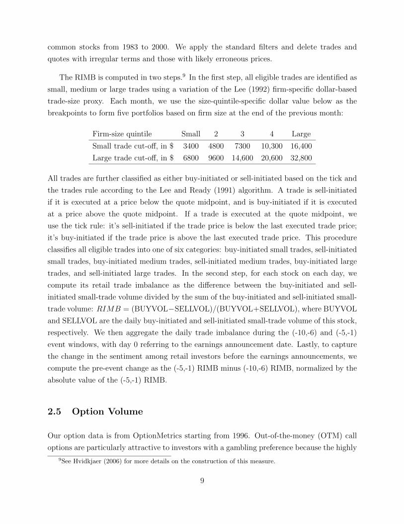
Figure 1 plots the difference of cumulative buy-and-hold excess returns between top and

bottom quintile portfolios based on lottery proxies over the (-5,+5) 11 trading days centered

around the earnings announcement dates. In particular, we calculate equal-weighted average

buy-and-hold excess returns accumulated starting from day -5. We plot the difference of the

average returns between the top and the bottom quintile lottery portfolios. For all six lottery

proxies, the returns of these hedge portfolios start to increase 5 days prior to the event date

and then decrease immediately after the event, with the biggest drop happening on the date

right after the event. Further, a similar pattern holds if we use the (-10,+10) 21 trading

12

days event window as shown in Figure 2. In sum, we provide information on when the

overvaluation of lottery-like stocks occurs in the first place, while most prior studies focus

on the subsequent reversals for lottery-like stocks.

We have documented an inverted-V shaped cumulative return spread based on lottery

proxies before and after earnings announcements in Figure 1. One might think that the

more intense speculative trading behavior may also hold for other anomaly characteristics,

and thus there is nothing special about our results for the inverted-V shaped cumulative

lottery spreads. Thus, for comparison, we also perform the same exercise for a set of other

anomaly-related characteristics. Probably the most well-known anomalies are value and

momentum. Recently, profitability and investment have also attracted a lot of attention. In

particular, Novy-Marx (2013), Fama and French (2015, 2016), and Hou, Xue, and Zhang

(2015) show that new factor models with additional factors related to profitability and

investment can account for a large set of asset pricing anomalies. Thus, we repeat our exercise

for value, momentum, profitability, and investment, and plot the cumulative anomaly return

spreads around the earnings announcements in Figure 3. First, the return spreads are more

pronounced around the earning announcements than in other periods, a finding consistent

with La Porta et al (1997) and Engelberg, McLean, and Pontiff (2015). More importantly,

the cumulative return spreads based on book-to-market, past returns, profitability and the

opposite of investment over assets increase both before and after earnings announcements.

It is worth noting that the shape for cumulative return spread in Figure 3 is monotonically

increasing, whereas for lottery characteristics, an inverted-V shape obtains. This contrast

highlights the unique role of speculation ahead of earnings announcements for our lottery-

related characteristics.

3.2 Fama-MacBeth Regressions

The portfolio approach in the previous section is simple and intuitive, but it cannot

explicitly control for other variables that may influence returns. To control for other firm

characteristics, we perform a series of Fama and MacBeth (1973) cross-sectional regressions.

In all of the Fama-MacBeth regressions below, we regress event-window excess returns

on a list of lagged traditional variables, such as firm size, book-to-market, and past returns.

Independent variables (except for returns) are winsorized at their cross-sectional 1st and

99th percentiles, and t-statistics are calculated based on the heteroskedasticity-consistent

standard errors of White (1980). Panel A of Table 3 reports the regressions during the

13

(-5,-1) pre-event window. Consistent with our prediction, the lottery proxy is positive and

significant for all six lottery proxies. Further, the regressions during the (0,+5) post-event

window reported in Panel B show the negative and significant predictive power of all lottery

measures as well. In particular, when the composite z-score increases by one standard

deviation, the pre-event 5-day return tends to increase by 0.188%, and the post-event 5-day

return tends to decrease by an even larger amount of 0.471%.

In sum, the evidence based on both the portfolio sorting approach and Fama-MacBeth

regressions is consistent with the notion that investors are especially attracted to lottery-like

stocks before earnings announcements, which generates positive lottery spreads that are in

the opposite direction from the traditional lottery anomalies.

4 Inspecting the Mechanisms

In this section, we provide further evidence of inventors’ gambling behavior before earnings

announcements. In particular, we will present results controlling for differences of opinion

as well as results from the retail trade imbalance and the trading behavior on the options

market.

4.1 Differences of Opinion

Berkman et al. (2009) also argue that speculative trading tends to increase prior to earnings

announcements. In addition, the Miller (1977) model suggests that stock prices are likely

to reflect optimists’ opinions due to short-sale impediments. Consequently, the net effect

of intensified speculative trading on prices is expected to be positive and should lead to

increasing overvaluation just ahead of earnings announcements. Moreover, because investors

who are more optimistic are more likely to take such speculative positions, the increase in

overvaluation should be larger for stocks with higher levels of differences of opinion. Based

on these arguments, Berkman et al. (2009) hypothesize that the price run-up during the

days leading up to earnings announcements for stocks with large differences of opinion should

be greater than those with small differences of opinion. Indeed, Berkman et al. (2009) find

supportive empirical evidence.

Lottery-like stocks might have more information uncertainty, which induces larger

14

differences of opinion among investors. Thus, to make sure that our results are not driven by

the potential correlation between our proxies for the lottery feature and differences of opinion,

we directly control for differences of opinion in Fama-MacBeth regressions. We adopt two

common proxies for differences of opinion: analyst forecast dispersion and turnover. Table 4

reports the results. Panel A adds analyst forecast dispersions before the announcements

and Panel B adds turnover in the previous month into the Fama-MacBeth regressions.

In the pre-event regressions, the lottery proxy is still positive and significant for all six

proxies, controlling for either analyst forecast dispersion or turnover. More interestingly,

the dispersion is not significant in any of the six pre-event regressions, suggesting that our

results cannot be explained by the differences of opinion story. Actually, our results indicate

that once lottery proxies are controlled, the level of differences of opinion is not positively

related to returns ahead of the earnings announcements, suggesting that the lottery effect

might play a role in the findings in Berkman et al (2009).12

Lastly, in untabulated analysis, we also replace the level of differences of opinion with

changes in differences of opinion ahead of the earnings announcements.13 We find that our

results remain quantitatively similar. In addition, since stocks with analyst coverage tend

to be larger, the evidence in Table 4 also indicates that our results hold for relatively large

stocks and are not completely driven by small stocks.

4.2 Evidence from Retail Trade Imbalance

Lottery preferences, like other behavioral biases, tend to be more prominent among individual

investors (see, e.g., Kumar (2009)). Therefore, we expect to see more trading initiated by

retail investors before earnings announcements, especially among lottery-like stocks. Table

5 compares the change in retail trade imbalance of lottery-like and non-lottery stocks prior

to the announcements. As shown in Panel A, there is indeed an increase in retail trade

12The main focus of Berkman et al. (2009) is on the more pronounced underperformance of stocks withhigh levels of differences of opinion around the earnings announcements due to reduction in disagreement,rather than the outperformance of these stocks ahead of earnings announcements. Thus, even if the lotteryeffect plays a significant role in their finding on the outperformance of high dispersion stocks ahead of earningsannouncements, it does not weaken the main argument and conclusion in Berkman et al. (2009).

13The reason that we control for changes in differences of opinion is the following. Differences of opinionmight be more severe before earnings announcements because of the high uncertainty during the pre-eventperiod. After the announcements, the uncertainty will be partly resolved as will be the differences ofopinion. Furthermore, this effect might be more pronounced for firms with large differences of opinion. Inother words, the change in the differences of opinion among investors has a similar time trend as the returnpattern we documented in the previous section in Figure 1. Coupled with short-sale constraints, this patternon differences of opinion could potentially explain our results.

15

imbalance for an average stock ahead of earnings announcements. Moreover, the increase in

retail trade imbalance is generally significantly larger among lottery-like stocks than among

non-lottery stocks.14

The more pronounced increases in retail trade imbalance on lottery-like stocks is likely

to lead to price increases of those stocks. When there is an imbalance between buy and sell

orders, market markers may absorb the order imbalance by serving as the trade counterparty.

However, market makers may demand greater compensation for incurring inventory risks

due to the greater anticipated volatility associated with the information event (see, e.g.,

Nagel (2012) and So and Wang (2015)). In addition, as discussed in the introduction,

arbitrage forces should also be more limited ahead of earnings announcements due to greater

uncertainty. Taken together, it implies a greater price run-up for lottery-like stocks ahead

of earnings announcements, consistent with our main findings in Table 2.

In light of the above discussion, we also study how retail trade imbalance affects returns

ahead earnings announcements. In Panel B, we use the regression approach where we include

the (-5,-1) RIMB and its interaction with lottery proxies along with all other controls in the

Fama-MacBeth regressions framework used by the previous section (i.e., Table 4, Panel

B). All the interaction terms between retail trade imbalance and lottery proxies appear to

be positive and significant, indicating that an increased retail investor interest before the

announcements tends to amplify the positive lottery spread before the announcements.

4.3 Evidence from the Option Markets

In addition to the direct evidence from investors’ trading behavior on the stock market,

we also examine whether the gambling preference exists in the options market and whether

it is intensified ahead of earnings announcements. OTM calls are a natural candidate for

gambling because they are cheap and have highly skewed payoffs. Therefore, if investors

have a stronger demand for lottery before the earnings announcements, they would be more

likely to buy short-term OTM calls prior to the event. We use the ATM calls on the same

stock as the benchmark, and plot the dynamics of the OTM call trading volume relative to

the ATM call trading volume during the (-5,+5) event window in Figure 4. As expected, the

relative trading volume starts to increase from 5 days prior to the event, peaks at the event

14In untabulated tests, we also conduct the same analysis for investors’ visits to company filings at theSEC Edgar website. We find a similar pattern that the lottery-like stocks experience significant increases ininvestors’ requests during the pre-event period.

16

date, and then sharply drops immediately after the event. This pre-event increase pattern

echoes that of the retail trade imbalance of the lottery-like stocks in the stock market.

In sum, the results from investors’ trading behavior on the stock market and the options

market provide further support for our hypothesis on investors’ amplified demand for lottery

ahead of earnings announcements.

4.4 Evidence from Religious Beliefs in Gambling Propensity

In this subsection, we examine the role of religious beliefs in gambling propensity. Kumar et

al. (2011) finds that there is geographic variation in religion-induced gambling preference,

and the lottery-stock premium is larger when a firm is located in a region with high

concentrations of Catholics relative to Protestants. Compared to the more tolerant gambling

views of Catholic churches, many Protestant churches have strong moral opposition to

gambling and consider it as a sinful activity.

Following their logic, if the speculative trading is due to lottery-like preferences, we

expect the effect to be stronger for firms in high CPRATIO regions as well. To test this

conjecture, we add the log of CPRATIO and its interaction with our lottery proxies into the

Fama-MacBeth regressions. Table 6 reports the results. Consistent with our prediction, the

interaction terms are all positive in the pre-event regressions and the sign completely flips

in the post-event regressions. That is, the inverted-V shaped pattern on cumulative return

spreads is more pronounced among firms in the regions with stronger gambling propensity.

4.5 Additional Robustness Checks

In this section, we report the results of several additional robustness tests.

First, we conduct a subsample analysis based on institutional ownership. Compared to

individual investors, institutional investors should be less subject to behavioral biases such as

lottery preference. Therefore, we perform a double-sorting portfolio analysis. Stocks are first

divided into 2 groups bases on the institutional ownership (IO) at the end of the previous

quarter, and then within each group, stocks are further divided into 5 portfolios based on

each one of the six lottery proxies from the month prior to the announcement date. If the

announcement date is in the first ten trading days of a month, we lag one more month for the

17

proxies. IO is defined as the percent of shares held by institutional investors as reported in

Thomson Financial 13F database. Table 7 reports the lottery spread within these subsamples

as well as their differences during the pre-event and post-event period. Consistent with our

conjecture, during the pre-event period, the lottery spreads are generally bigger within the

bottom 50% IO subsample, and the difference between top and bottom IO group is significant

for four of the six proxies. A similar pattern also appears during the post-event period, where

the underperformance of lottery-like stocks is more severe among the low IO subsample, with

the difference-in-differences significant for four of the six proxies.

Second, we examine the international data to see whether the results we documented

are an international phenomenon. We repeat the analysis in Table 2 for other non-US

G7 countries. For each country, we construct a composite z-score based on three lottery

proxies, Maxret, Prc, and IVOL.15 Table 8 shows that the same pattern emerges for most

G7 countries. In particular, the return spread between lottery-like and non-lottery stocks

before earnings announcements are 0.66%, 1.20%, 0.51%, 0.27%, -0.46%, 0.02% for Canada,

Germany, France, UK, Italy, and Japan, respectively. In contrast, the return spread between

lottery-like and non-lottery stocks after earnings announcements are -0.58%, -0.93%, -0.66%,

-1.66%, -0.94%, and -1.16% in these countries. Further, we plot the difference of cumulative

buy-and-hold excess returns between top and bottom quintile portfolios based on the

composite z-score over the (-5,+5) 11 trading days centered around earnings announcements

for non-US G7 countries in Figure 5. A similar pattern to our US Figure 1 emerges: except

for Italy, the returns of these hedge portfolios start to increase 5 days prior to the event date

and then decrease immediately after the event, with the biggest drop happening on the day

right after the event.16

Our third robustness test examines the realized return skewness of lottery-like and non-

lottery stocks during the event window. Lottery-like stocks tend to have higher skewness than

non-lottery stocks on average. More importantly, investors might believe that the differences

in skewness between lottery-like and non-lottery stocks are particularly large during the

earnings announcement periods as compared to other periods. Thus, investors prefer lottery-

15The data to construct the other two lottery proxies are limited, thus we only use these three easy-to-calculate proxies to compute our composite z-score for international stocks. To calculate IVOL for other G7countries, we first construct a local market three-factor model following Gao et al (2015), and then IVOL isthe standard deviation of residuals from daily three-factor regressions. More details on international dataare provided in the Appendix.

16U.K. shows a different pattern from other countries at day 0 because of its different earnings reportschedule. Unlike US firms which typically report either before the start of trading or after the closing bell,most U.K. companies report their earnings at 7am London time.

18

like stocks more strongly before earnings announcements. To test this prediction, we

calculate the realized skewness between top and bottom quintile lottery portfolios during

both the actual-event period and the pseudo-event period, and compare the difference-in-

differences. Panel A of Table 9 reports the results. As expected, the (-1,+1) event-window

returns of lottery-like stocks have higher skewness than non-lottery stocks on average. In

addition, lottery-like stocks have much higher realized skewness during the event window

than during other times, while the skewness for non-lottery stocks is similar across the

event window and the non-event window. More important, the difference-in-differences of

skewness are higher during event periods than other periods for all six proxies. Further,

apart from return skewness, we also examine the realized skewness of earnings surprises on

announcement dates. Panel B of Table 9 reports the results. For all six lottery proxies, the

realized skewness of earnings surprises is also much higher among lottery-like stocks than

non-lottery stocks.

Our fourth robustness test investigates the lottery return spread around earnings

announcements among the subsample of early, on-time, and late announcers. Some firms

make earnings announcements earlier than the expected dates, while others are later than

the expected dates. Earlier studies find that early announcers tend to have good news while

late announcers tend to have bad news (e.g., Givoly and Palmon (1982), Chambers and

Penman (1984), Bagnoli, Kross, and Watts (2002) and Johnson and So (2016)). When some

investors anticipate good news, they might have an even stronger demand for lottery-like

stocks, and thus lead to a higher lottery return spread. Furthermore, advancers tend to

receive more positive media attention than delayers. Thus, due to greater attention ahead

of earnings announcements, the lottery return spreads might be larger as well among earlier

announcers.

To perform a formal test, we repeat the exercise in Table 2 within the subsample of

early, on-time, and late announcers relative to the expected earnings announcement dates.

Following So and Wang (2015), expected earnings announcement dates are calculated by

adding the historical reporting lag to the current fiscal quarter end. The historical reporting

lag is the median number of trading days between a firm’s fiscal quarter end and its actual

announcement date for the same fiscal quarter over the previous ten years. Early, on-time,

and late announcers are firms whose actual announcement dates are more than one day

before, within one day, and more than one day after the expected earnings announcement

dates, respectively.

We report the time series average of excess returns of these lottery portfolios and

19

the differences between top and bottom quintile portfolios around the expected earnings

announcement window within the subsample of early, on-time, and late announcers relative

to the expected earnings announcement dates. The results in Table 10 indicate that the

positive lottery return spreads are largest among early announcers, moderate among on-time

announcers, and the weakest among late announcers.17 This evidence is consistent with the

fact that early announcers tend to have good news and more positive media coverage while

late announcers tend to have bad news and less positive media attention. Anticipating the

good news (at least by some investors), the stronger demand for lottery-like stocks might

be amplified even further, thus leading to a larger lottery return spread ahead of earning

news among earlier announcers. On the other hand, for late announcers, in anticipation of

bad news, investors may shy away from the lottery-like stocks, and thus we do not observe a

positive lottery return spread before earnings announcements among these late announcers.

Lastly, in untabulated analysis, we repeat the exercise in Table 10 among the subsample

of firms with ex post good earnings news, ex post no earning surprise, and ex post bad

earnings news. If part of the earnings news is leaked or anticipated by some investors, then

we should observe a similar pattern: the lottery return spreads ahead of earnings news should

be strongest among firms with ex post good news, moderate among firms with no surprise,

and weakest among firms with ex post bad news. Indeed, our untabulated analysis confirms

this conjecture.

5 Refined Lottery Strategy

Given our previous findings on the different return patterns of lottery-like stocks before and

after earnings announcements, we propose a refined lottery strategy and compare it with the

standard lottery strategy in this section.

Since lottery-like stocks underperform non-lottery stocks on average, the standard lottery

strategy typically holds a hedge portfolio which buys non-lottery stocks and sells lottery-

like stocks. Given our findings in the previous sections that lottery-like stocks actually

outperform non-lottery stocks before earnings announcements, we therefore propose a refined

lottery strategy of buying lottery-like stocks and selling non-lottery stocks during the (-10,-1)

pre-event window, and then reverting to the standard lottery strategy afterwards. To ensure

17The opposite pattern for the post event window is partially driven by the standard post earningsannouncements drifts since the lottery-like stocks tend to have more negative surprise among late announcersthan among earlier announcers.

20

that the strategy is implementable, we only use the pre-event dates in the same month of

the actual announcement date. In other words, instead of longing non-lottery stocks and

shorting lottery-like stocks during the entire month t after forming lottery portfolios at the

end of month t − 1 as in the standard lottery strategy, for stocks with scheduled earnings

announcements in month t, we sell the stock if it belongs to the bottom lottery quintile,

or buy the stock if it’s in the top lottery quintile, during the (-10,-1) pre-event window.

Further, if the earnings announcement date is in the first ten trading days of month t, in

which case some dates of the (-10,-1) pre-event window are actually in month t− 1, we skip

these pre-event dates in month t− 1 and only adopt this reverse strategy for those pre-event

dates in month t after the portfolio formation at the end of month t− 1.

Table 11 reports the value-weighted excess returns and Fama-French four-factor alphas

for monthly quintile portfolios under the standard lottery strategy (Panel A) and our

refined strategy (Panel B) as well as their differences (Panel C). While the standard lottery

strategies achieve a positive and significant alpha for four of six proxies, our new strategies

significantly increase these return spreads. Take the composite Z-score as an example. Our

new strategy improves the long-short portfolio performance by about 38% by increasing the

average monthly Fama-French four-factor alpha from 1.09% to 1.50%, with the t-stat of

the difference-in-differences equal to 2.48. In untabulated analysis, we use equally weighted

portfolio strategies instead of value-weighted strategies, and we find that the improvement

is even more statistically significant. Nonetheless, an important caveat is that in reality the

improvement might be much smaller due to higher transaction costs associated with this

new strategy.

6 Conclusion

In this paper, we argue that investors’ preferences for lottery/gambling are time varying,

and are especially strong ahead of earnings news, probably due to lower inventory costs for

speculators. On the other hand, the countervailing arbitrage forces are more limited due

to elevated uncertainty leading to the earnings news. Taken together, we expect that there

should be positive return spreads between lottery-like assets and non-lottery assets during

the days ahead of earnings announcements. Indeed, we document that the return spreads

between lottery-like assets and non-lottery assets have opposite patterns before and after

earnings announcements. Most prior studies show that lottery-like stocks can be overvalued

and focus on the subsequent return reversal of the lottery-like stocks. Thus, our focus

21

on earnings announcements identifies the periods when the overvaluation of the lottery-like

stocks is occurring, rather than their subsequent corrections as studied by most prior studies.

Our empirical findings are robust across six different proxies that are studied in the

literature of lottery-related anomalies. In addition, this inverted-V shaped pattern on lottery

return spreads is more pronounced among firms with more retail trade imbalance, with low

institutional ownership, and in the regions with stronger gambling propensity. Moreover, we

show that the cumulative return spreads based on other anomalies characteristics such as

book-to-market, past returns, profitability and minus investment over assets are increasing

both before and after earnings announcements. Thus, the inverted-V shaped cumulative

return spread is unique to lottery-related characteristics. This sharp contrast in the shape

of cumulative return spreads highlights the unique role of speculation ahead of earnings

announcements for our lottery-related characteristics.

22

References

An, Li, Huijun Wang, Jian Wang, Jianfeng Yu, 2016. Lottery-related anomalies: the roleof reference-dependent preferences. Unpublished working paper. Tsinghua University,University of Delaware, Chinese University of Hong Kong (Shenzhen), and University ofMinnesota.

Anderson, Anne-Marie, Edward A. Dyl, 2005, Market structure and trading volume, Journalof Financial Research 28, 115–131.

Ang, Andrew, Robert J. Hodrick, Yuhang Xing, and Xiaoyan Zhang, 2006, The cross-sectionof volatility and expected returns, Journal of Finance 61, 259–299.

Ang, Andrew, Robert J. Hodrick, Yuhang Xing, and Xiaoyan Zhang, 2009, High idiosyncraticvolatility and low returns: International and further U.S. evidence, Journal of FinancialEconomics 91, 1–23.

Bagnoli, Mark, William Kross, and Susan G. Watts, 2002, The information in management’sexpected earnings report date: a day late, a penny short, Journal of Accounting Research40(5), 1275–1296.

Bali, Turan, Stephen Brown, Scott Murray, and Yi Yang, 2014, A lottery demand-basedexplanation of the beta anomaly, Working paper, Georgetown University.

Bali, Turan, Nusret Cakici, and Robert Whitelaw, 2011, Maxing out: Stocks as lotteries andthe cross-section of expected returns, Journal of Financial Economics 99, 427–446.

Bali, Turan and Scott Murray, 2013, Does risk-neutral skewness predict the cross-sectionof equity option portfolio returns? Journal of Financial and Quantitative Analysis 48,1145–1171.

Barber, Brad, Terrance Odean, and Ning Zhu, 2009, Do retail trades move markets?, Reviewof Financial Studies 22, 151–186.

Barberis, Nicholas, and Ming Huang, 2008, Stocks as lotteries: The implications ofprobability weighting for security prices, American Economic Review 98, 2066–2100.

Berkman, Henk, Valentin Dimitrov, Prem Jain, Paul Koch, and Sheri Tice, 2009, Sell onthe news: Differences of opinion, short-sales constraints, and returns around earningsannouncements, Journal of Financial Economics 92, 376–399.

Boulland, Romain, and Olivier Dessaint, 2014, Announcing the announcement, WorkingPaper, ESSEC Business School.

Boyer, Brian, Todd Mitton, and Keith Vorkink, 2010, Expected idiosyncratic skewness,Review of Financial Studies 23, 169–202.

23

Brunnermeier, Markus K., Christian Gollier, and Jonathan A. Parker, 2007, Optimal beliefs,asset prices, and the preference for skewed returns, American Economic Review 97(2),159–165.

Chambers, Anne, and Stephen Penman, 1984, Timeliness of reporting and the stock pricereaction to earnings announcements, Journal of Accounting Research 22(1), 21–47.

Conrad, Jennifer, Robert Dittmar, and Eric Ghysels, 2013, Ex ante skewness and expectedstock returns, Journal of Finance 68, 85–124.

Conrad, Jennifer, Nishad Kapadia and Yuhang Xing, 2014, Death and jackpot: Why doindividual investors hold overpriced stocks?, Journal of Financial Economics 113, 455–475.

Doran, James, Danling Jiang, and David Peterson, 2011, Gambling preference and the newyear effect of assets with lottery features, Review of Finance 16(3), 685–731.

Engelberg, Joseph, David McLean, and Jeffery Pontiff, 2015, Anomalies and news, Workingpaper UCSD.

Fama, Eugene, and James MacBeth, 1973, Risk, return, and equilibrium: Empirical tests,Journal of Political Economy 81, 607–636.

Fama, Eugene, and Kenneth R. French, 1993, Common risk factors in the returns on stocksand bonds, Journal of Financial Economics 47, 427–465.

Fama, Eugene, and Kenneth R. French, 2012, Size, value, and momentum in internationalstock returns, Journal of Financial Economics 33, 3–56.

Fama, Eugene, and Kenneth R. French, 2015, A five-factor asset pricing model, Journal ofFinancial Economics 116, 1–22.

Fama, Eugene, and Kenneth R. French, 2016, Choosing factors, Working paper, Universityof Chicago and Dartmonth College.

Fox, Craig, 1999, Strength of evidence, judged probability, and choice under uncertainty,Cognitive Psychology 38, 167–189.

Gao, Pengjie, Christopher Parsons, and Jianfeng Shen, 2015, The global relation betweenfinancial distress and equity returns, Working Paper, University of Notre Dame, UCSD,and UNSW.

Givoly, Dan and Dan Palmon, 1982, Timeliness of actual earnings announcements: Someempirical evidence, The Accounting Review 57, 486–508.

Green, Clifton and Byoung Hwang, 2012, Initial public offerings as lotteries: Skewnesspreference and first-day returns, Management Science 58, 432–44.

24

Hilary, Gilles, and Kai Wai Hui, 2009, Does religious matter in corporate decision makingin America?, Journal of Financial Economics 93, 455–473.

Hvidkjaer, Soeren, 2006, A trade-based analysis of momentum, Review of Financial Studies19, 457–491.

Hou, Kewei, Chen Xu, and Lu Zhang, 2015, Digesting anomalies: An investment approach,Review of Financial Studies 28, 650–705.

Johnson, Travis L., and Eric So, 2016, Time will tell: Information in the timing of scheduledearnings news, Working Paper University of Texas and MIT.

Kumar, Alok, 2009, Who gambles in the stock market? Journal of Finance 64, 1889–1933.

Kumar, Alok, Jeremy Page, and Oliver Spalt, 2011, Religious beliefs, gamling attitudes, andfinancial market outcomes, Journal of Financial Economics 102, 671–708.

La Porta, Rafael, Josef Lakonishok, Andrei Shleifer, and Robert Vishny, 1997, Good newsfor value stocks: Further evidence on market efficiency, Journal of Finance 52, 859-874.

Lee, Charles, 1992, Earnings news and small trades, Journal of Accounting and Economics15, 265–302.

Lee, Charles, and Mark Ready, 1991, Inferring trade direction from intraday data, Journalof Finance 46(2), 733–746.

Livnat, Joshua, and Richard Mendenhall, 2006, Comparing the post-earnings announcementdrift for surprises calculated from analyst and time series forecasts, Journal of AccountingResearch 44(1), 177–205.

Mendenhall, Richard, 2004, Arbitrage risk and post-earnings-announcement drift, Journalof Bueiness 77(4), 875–894.

Miller, Edward, 1977, Risk, uncertainty and divergence of opinion, Journal of Finance 32,1151–1168.

Nagel, Stefan, 2012, Evaporating liquidity, Review of Financial Studies 25, 2005–2039.

Norvy-Marx, Robert, 2013, The other side of value: The gross profitability premium, Journalof Financial Economics 108, 1–28.

Newey, Whitney K., and Kenneth D. West, 1987, A simple, positive semi-definite,heteroskedasticity and autocorrelation consistent covariance matrix, Econometrica 55,703–708.

Rosch, Dominik, Avanidhar Subrahmanyam, and Mathijs A. Van Dijk, 2016, The dynamicsof market efficiency, Review of Financial Studies forthcoming.

So, Eric, and Sean Wang, 2014, News-driven return reversals: Liquidity provision ahead of

25

earnings announcements, Journal of Financial Economics 114, 20–35.

White, Halbert, 1980, A heteroskedasticity-consistent covariance matrix estimator and adirect test for heteroskedasticity, Econometrica 48, 817–838.

Xing, Yuhang, Xiaoyan Zhang, and Rui Zhao, 2010, What does individual option volatility

smirk tell us about future equity returns?, Journal of Financial and Quantitative Analysis

45, 641–662.

26

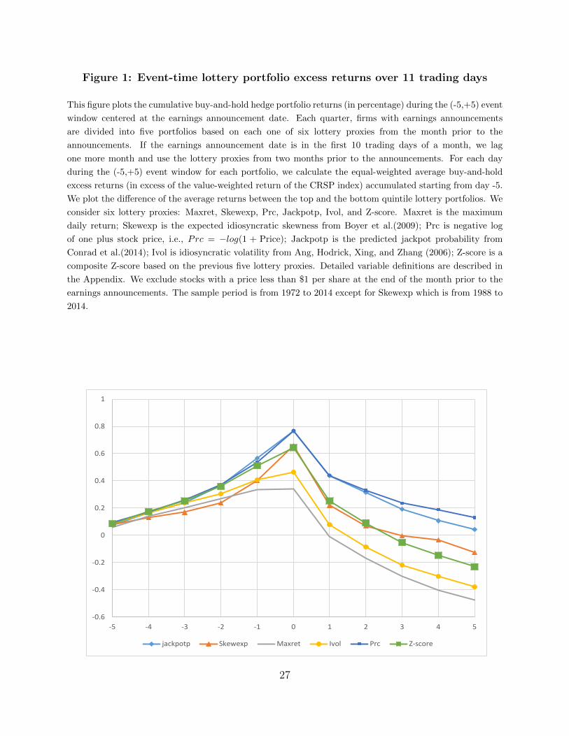
Figure 1: Event-time lottery portfolio excess returns over 11 trading days

This figure plots the cumulative buy-and-hold hedge portfolio returns (in percentage) during the (-5,+5) event

window centered at the earnings announcement date. Each quarter, firms with earnings announcements

are divided into five portfolios based on each one of six lottery proxies from the month prior to the

announcements. If the earnings announcement date is in the first 10 trading days of a month, we lag

one more month and use the lottery proxies from two months prior to the announcements. For each day

during the (-5,+5) event window for each portfolio, we calculate the equal-weighted average buy-and-hold

excess returns (in excess of the value-weighted return of the CRSP index) accumulated starting from day -5.

We plot the difference of the average returns between the top and the bottom quintile lottery portfolios. We

consider six lottery proxies: Maxret, Skewexp, Prc, Jackpotp, Ivol, and Z-score. Maxret is the maximum

daily return; Skewexp is the expected idiosyncratic skewness from Boyer et al.(2009); Prc is negative log

of one plus stock price, i.e., Prc = −log(1 + Price); Jackpotp is the predicted jackpot probability from

Conrad et al.(2014); Ivol is idiosyncratic volatility from Ang, Hodrick, Xing, and Zhang (2006); Z-score is a

composite Z-score based on the previous five lottery proxies. Detailed variable definitions are described in

the Appendix. We exclude stocks with a price less than $1 per share at the end of the month prior to the

earnings announcements. The sample period is from 1972 to 2014 except for Skewexp which is from 1988 to

2014.

-0.6

-0.4

-0.2

0

0.2

0.4

0.6

0.8

1

-5 -4 -3 -2 -1 0 1 2 3 4 5

jackpotp Skewexp Maxret Ivol Prc Z-score

27

Figure 2: Event-time lottery portfolio excess returns over 21 trading days

This figure plots the cumulative buy-and-hold hedge portfolio returns (in percentage) during the (-10,+10)

event window centered at the earnings announcement date. Each quarter, firms with earnings announcements

are divided into five portfolios based on each one of six lottery proxies from the month prior to the

announcements. If the earnings announcement date is in the first 10 trading days of a month, we lag

one more month and use the lottery proxies from two months prior to the announcements. For each day

during the (-10,+10) event window for each portfolio, we calculate the equal-weighted average buy-and-hold

excess returns (in excess of the value-weighted return of the CRSP index) accumulated starting from day

-10. We plot the difference of the average returns between the top and the bottom quintile lottery portfolios.

Lottery proxies are defined the same as in Figure 1. We exclude stocks with a price less than $1 per share at

the end of the month prior to the earnings announcements. The sample period is from 1972 to 2014 except

for Skewexp which is from 1988 to 2014.

-1

-0.8

-0.6

-0.4

-0.2

0

0.2

0.4

0.6

0.8

1

-10 -8 -6 -4 -2 0 2 4 6 8 10

Jackpotp Skewexp Maxret Ivol Prc Z-score

28

Figure 3: Event-time portfolio excess returns over 11 trading days

This figure plots the cumulative buy-and-hold hedge portfolio returns (in percentage) during the (-5,+5) event

window centered at the earnings announcement date. Each quarter, firms with earnings announcements are

divided into five portfolios based on each one of four proxies from the month prior to the announcements:

Book-to-market equity (B/M), Momentum (MOM), Profitability (ROA), and the opposite of Investment-to-

assets (-IA). If the earnings announcement date is in the first 10 trading days of a month, we lag one more

month and use the proxies from two months prior to the announcements. For each day during the (-5,+5)

event window for each portfolio, we calculate the equal-weighted average buy-and-hold excess returns (in

excess of the value-weighted return of the CRSP index) accumulated starting from day -5, and plot the

difference of the average returns between the top and the bottom quintile portfolios. BM is the book value

of equity divided by market value at the end of the last fiscal year. MOM is the cumulative stock return

over the past year skipping one month. ROA is quarterly earnings divided by total assets in the previous

quarter. IA is the annual change in total assets divided by total assets in the previous year. We exclude

stocks with a price less than $1 per share at the end of the month prior to the earnings announcements. The

sample period is from 1972 to 2014.

0

0.1

0.2

0.3

0.4

0.5

0.6

0.7

0.8

0.9

1

-5 -4 -3 -2 -1 0 1 2 3 4 5

B/M -IA ROA MOM

29

Figure 4: Event-time aggregate call options trading volume spread

This figure plots the daily adjusted volume spread of short-term OTM call options relative to ATM call

options during the (-5,+5) event window centered at the earnings announcement date. We only use short-

term options expiring in the next month. The adjusted volume for OTM (ATM) calls is defined as the

percentage change of daily OTM (ATM) volume from its 3-month moving average, and the adjusted volume

spread is the difference between the adjusted volume of OTM and ATM calls. The sample period is from

1996 to 2014.

0

0.1

0.2

0.3

0.4

0.5

0.6

0.7

0.8

0.9

-5 -4 -3 -2 -1 0 1 2 3 4 5

OT

M-A

TM

Vo

lum

e

Day relative to earnings announcement

30

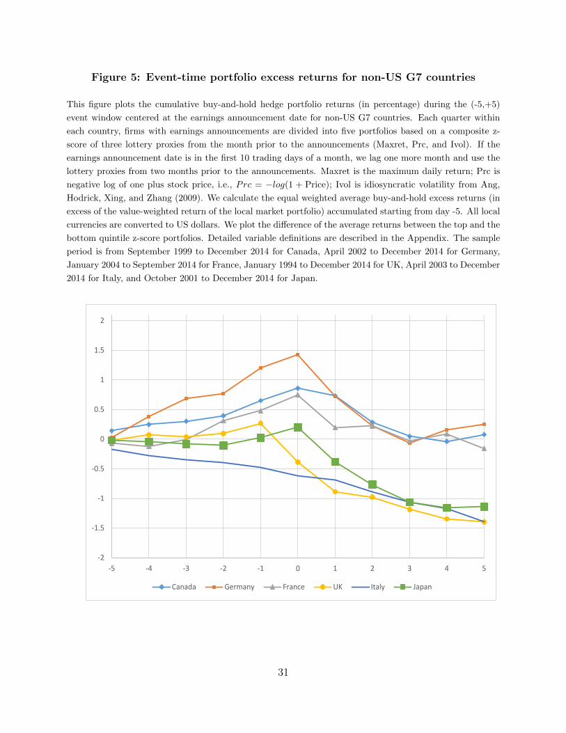
Figure 5: Event-time portfolio excess returns for non-US G7 countries

This figure plots the cumulative buy-and-hold hedge portfolio returns (in percentage) during the (-5,+5)

event window centered at the earnings announcement date for non-US G7 countries. Each quarter within

each country, firms with earnings announcements are divided into five portfolios based on a composite z-

score of three lottery proxies from the month prior to the announcements (Maxret, Prc, and Ivol). If the

earnings announcement date is in the first 10 trading days of a month, we lag one more month and use the

lottery proxies from two months prior to the announcements. Maxret is the maximum daily return; Prc is

negative log of one plus stock price, i.e., Prc = −log(1 + Price); Ivol is idiosyncratic volatility from Ang,

Hodrick, Xing, and Zhang (2009). We calculate the equal weighted average buy-and-hold excess returns (in

excess of the value-weighted return of the local market portfolio) accumulated starting from day -5. All local

currencies are converted to US dollars. We plot the difference of the average returns between the top and the

bottom quintile z-score portfolios. Detailed variable definitions are described in the Appendix. The sample

period is from September 1999 to December 2014 for Canada, April 2002 to December 2014 for Germany,

January 2004 to September 2014 for France, January 1994 to December 2014 for UK, April 2003 to December

2014 for Italy, and October 2001 to December 2014 for Japan.

-2

-1.5

-1

-0.5

0

0.5

1

1.5

2

-5 -4 -3 -2 -1 0 1 2 3 4 5

Canada Germany France UK Italy Japan

31

Table 1: Summary Statistics

This table reports the summary statistics for our sample of firm-quarter observations. EXRET (−1,+1),

EXRET (−5,−1), and EXRET (0,+5), are the buy-and-hold excess returns for (-1,+1), (-5,-1), (0,+5)

three relevant earnings announcement window periods, respectively, with day 0 referring to the earnings

announcement date. The excess return is the difference between stock return and the return of the value-

weighted CRSP index. ME is the market value of equity in millions, and MB is ME divided by the book value

of equity, both measured at the end of the prior fiscal quarter. Momentum (MOM(−12,−1)) is cumulative

stock returns over the past year skipping one month. Turnover is monthly trading volume divided by the

number of shares outstanding. To address the issue of double counting of volume for NASDAQ stocks, we

follow Anderson and Dyl (2005) and scale down the volume of NASDAQ stocks by 50% before 1997 and

38% after 1997 to make it roughly comparable to the volume on the NYSE. We consider six lottery proxies:

Maxret is the maximum daily return, Skewexp is the expected idiosyncratic skewness from Boyer et al.(2009),

Price is month-end stock price, Jackpotp is the predicted jackpot probability from Conrad et al.(2014), and

Ivol is the standard deviation of daily residual returns relative to the Fama and French (1993) three-factor

model from Ang, Hodrick, Xing, and Zhang (2006). Z-score is a composite Z-score based on the previous

five lottery proxies. Detailed variable definitions are described in the Appendix. We exclude stocks with a

price less than $1 per share at the end of the month prior to the earnings announcements. All continuous

variables (except returns) are winsorized cross-sectionally at the 1st and 99th percentiles. The sample period

is from 1972 to 2014 except for Skewexp which is from 1988 to 2014. Variables are reported in percentages

except for ME, MB, Skewexp, Price, and Z-score.

Summary Statistics

Mean Std Q1 Median Q3EXRET(-1,+1) 0.204 8.708 -3.384 -0.075 3.414EXRET(-5,-1) 0.331 7.819 -3.128 -0.113 3.093EXRET(0,+5) -0.028 10.472 -4.588 -0.357 3.957ME 1496.112 5707.589 39.791 151.830 684.693MB 2.862 4.492 1.026 1.672 2.923MOM(-12,-1) 0.167 0.733 -0.178 0.067 0.346Turnover 7.432 10.078 1.631 3.938 9.078Maxret 6.869 5.865 3.150 5.128 8.499Skewexp 0.750 0.598 0.332 0.653 1.092Price 19.505 18.312 6.375 14.375 26.750Jackpotp 1.818 3.071 0.534 1.052 1.989Ivol 2.612 1.915 1.303 2.061 3.305Z-score -0.059 0.838 -0.764 -0.112 0.612

32

Table 2: Pre-event and Post-event Portfolio Returns

Each quarter, firms with earnings announcements in that quarter are sorted into five portfolios based on

each one of six lottery proxies from the month prior to the announcement date. If the announcement date is

in the first ten trading days of a month, we lag one more month for the proxies. We report equal-weighted

excess returns of these lottery portfolios, and the differences between top and bottom quintile portfolios

during the (-5,-1) pre-event period in Panel A.1 and the (0,+5) post-event period in Panel B.1, with day 0

referring to the earnings announcement date. Panel A.2 and B.2 present analogous average returns using

pseudo-announcement dates. Pseudo-announcement dates are computed by subtracting a randomly selected

number of trading days from the actual announcement date, where the random numbers are drawn from a

uniform distribution spanning 10 to 40 days. Panel A.3 and B.3 compare the differences between actual- and

pseudo-announcement dates. Lottery proxies are defined the same as in Table 1. We exclude stocks with

a price less than $1 per share at the end of the month prior to the earnings announcements. The sample

period is from 1972 to 2014 except for Skewexp which is from 1988 to 2014. Excess returns are reported

in percentages. The t-statistics are calculated based on the heteroskedasticity-consistent standard errors of

White (1980).

Panel A: (-5,-1) Pre-event Excess Return

Proxy= Maxret Skewexp Prc Jackpotp Ivol Z-scorePanel A.1: Actual dates

Q1 0.114 0.219 0.147 0.075 0.096 0.065Q2 0.207 0.218 0.175 0.173 0.171 0.212Q3 0.311 0.230 0.192 0.297 0.317 0.266Q4 0.427 0.420 0.309 0.466 0.418 0.384Q5 0.452 0.627 0.689 0.646 0.509 0.583Q5-Q1 0.339 0.408 0.542 0.570 0.413 0.518t-stat (3.46) (3.67) (5.79) (5.19) (3.83) (4.71)

Panel A.2: Pseudo datesQ1 0.057 0.013 0.025 0.012 0.047 0.049Q2 0.042 0.034 -0.026 0.041 0.053 0.033Q3 0.072 0.051 0.033 0.056 0.065 0.038Q4 0.049 0.060 0.014 0.043 0.037 0.036Q5 -0.008 0.043 0.167 0.082 0.010 0.042Q5-Q1 -0.064 0.030 0.141 0.071 -0.036 -0.007t-stat (-0.91) (0.31) (1.71) (0.80) (-0.45) (-0.08)

Panel A.3: Actual dates minus Pseudo datesQ1 0.057 0.206 0.122 0.064 0.049 0.016Q2 0.164 0.185 0.201 0.132 0.118 0.179Q3 0.239 0.178 0.158 0.241 0.252 0.228Q4 0.379 0.359 0.295 0.423 0.381 0.348Q5 0.460 0.584 0.522 0.564 0.499 0.541Q5-Q1 0.403 0.378 0.401 0.500 0.450 0.525t-stat (4.34) (3.00) (4.57) (4.96) (4.33) (5.17)

33

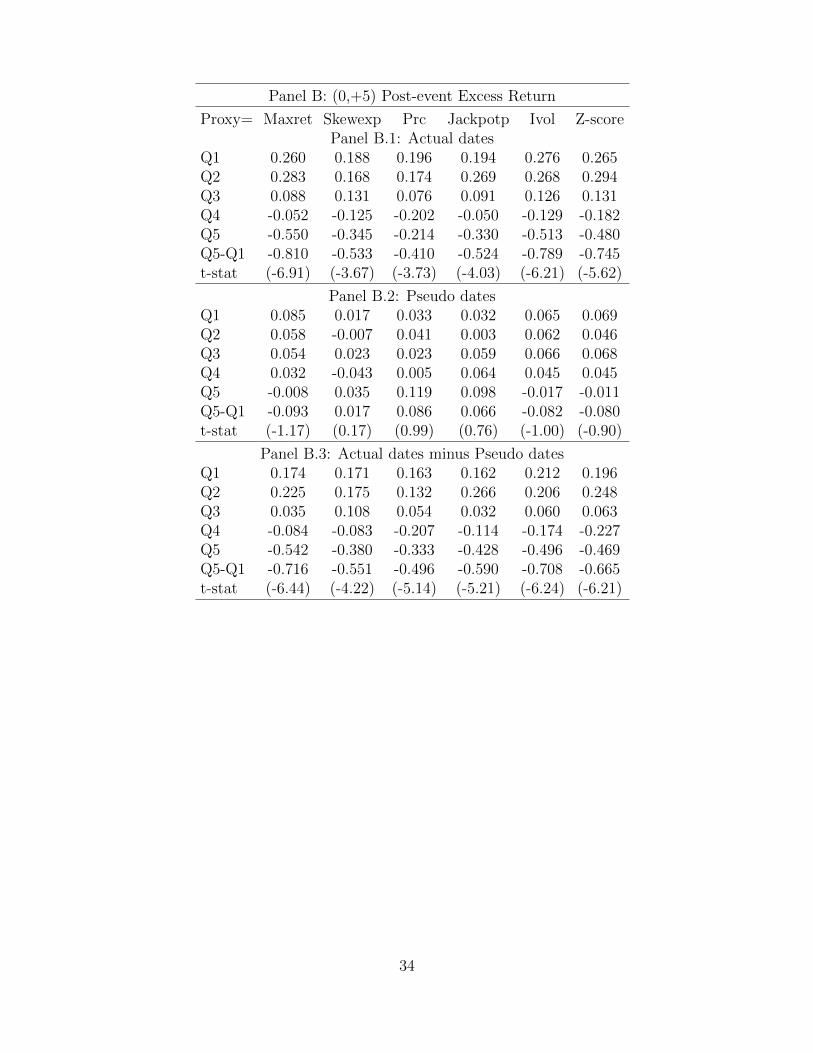
Panel B: (0,+5) Post-event Excess Return

Proxy= Maxret Skewexp Prc Jackpotp Ivol Z-scorePanel B.1: Actual dates

Q1 0.260 0.188 0.196 0.194 0.276 0.265Q2 0.283 0.168 0.174 0.269 0.268 0.294Q3 0.088 0.131 0.076 0.091 0.126 0.131Q4 -0.052 -0.125 -0.202 -0.050 -0.129 -0.182Q5 -0.550 -0.345 -0.214 -0.330 -0.513 -0.480Q5-Q1 -0.810 -0.533 -0.410 -0.524 -0.789 -0.745t-stat (-6.91) (-3.67) (-3.73) (-4.03) (-6.21) (-5.62)

Panel B.2: Pseudo datesQ1 0.085 0.017 0.033 0.032 0.065 0.069Q2 0.058 -0.007 0.041 0.003 0.062 0.046Q3 0.054 0.023 0.023 0.059 0.066 0.068Q4 0.032 -0.043 0.005 0.064 0.045 0.045Q5 -0.008 0.035 0.119 0.098 -0.017 -0.011Q5-Q1 -0.093 0.017 0.086 0.066 -0.082 -0.080t-stat (-1.17) (0.17) (0.99) (0.76) (-1.00) (-0.90)

Panel B.3: Actual dates minus Pseudo datesQ1 0.174 0.171 0.163 0.162 0.212 0.196Q2 0.225 0.175 0.132 0.266 0.206 0.248Q3 0.035 0.108 0.054 0.032 0.060 0.063Q4 -0.084 -0.083 -0.207 -0.114 -0.174 -0.227Q5 -0.542 -0.380 -0.333 -0.428 -0.496 -0.469Q5-Q1 -0.716 -0.551 -0.496 -0.590 -0.708 -0.665t-stat (-6.44) (-4.22) (-5.14) (-5.21) (-6.24) (-6.21)

34

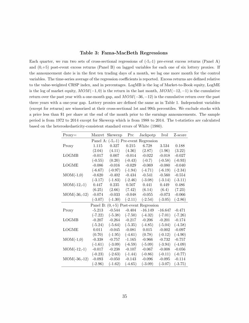
Table 3: Fama-MacBeth Regressions

Each quarter, we run two sets of cross-sectional regressions of (-5,-1) pre-event excess returns (Panel A)

and (0,+5) post-event excess returns (Panel B) on lagged variables for each one of six lottery proxies. If

the announcement date is in the first ten trading days of a month, we lag one more month for the control

variables. The time-series average of the regression coefficients is reported. Excess returns are defined relative

to the value-weighted CRSP index, and in percentages. LogMB is the log of Market-to-Book equity, LogME

is the log of market equity, MOM(−1, 0) is the return in the last month, MOM(−12,−1) is the cumulative

return over the past year with a one-month gap, and MOM(−36,−12) is the cumulative return over the past

three years with a one-year gap. Lottery proxies are defined the same as in Table 1. Independent variables

(except for returns) are winsorized at their cross-sectional 1st and 99th percentiles. We exclude stocks with

a price less than $1 per share at the end of the month prior to the earnings announcements. The sample

period is from 1972 to 2014 except for Skewexp which is from 1988 to 2014. The t-statistics are calculated

based on the heteroskedasticity-consistent standard errors of White (1980).

Proxy= Maxret Skewexp Prc Jackpotp Ivol Z-score

Panel A: (-5,-1) Pre-event RegressionProxy 1.115 0.327 0.215 6.728 3.534 0.188

(2.04) (4.11) (4.36) (2.87) (1.96) (3.22)LOGMB -0.017 0.007 -0.014 -0.022 -0.018 -0.027

(-0.55) (0.20) (-0.43) (-0.7) (-0.58) (-0.93)LOGME -0.086 -0.016 -0.029 -0.069 -0.080 -0.040

(-6.67) (-0.97) (-1.94) (-4.71) (-6.19) (-2.34)MOM(-1,0) -0.620 -0.402 -0.434 -0.541 -0.560 -0.554

(-3.17) (-1.83) (-2.46) (-3.08) (-3.14) (-3.11)MOM(-12,-1) 0.447 0.235 0.507 0.441 0.449 0.486

(6.25) (2.66) (7.42) (6.14) (6.4) (7.23)MOM(-36,-12) -0.074 -0.033 -0.048 -0.055 -0.073 -0.066

(-3.07) (-1.30) (-2.11) (-2.54) (-3.05) (-2.86)

Panel B: (0,+5) Post-event RegressionProxy -5.213 -0.544 -0.404 -16.149 -16.647 -0.471

(-7.22) (-5.38) (-7.50) (-4.32) (-7.01) (-7.26)LOGMB -0.207 -0.264 -0.217 -0.206 -0.201 -0.174

(-5.24) (-5.64) (-5.35) (-4.85) (-5.04) (-4.58)LOGME 0.011 -0.045 -0.081 0.015 -0.002 -0.097

(0.70) (-1.95) (-4.61) (0.78) (-0.12) (-4.90)MOM(-1,0) -0.338 -0.757 -1.165 -0.966 -0.732 -0.757

(-1.61) (-3.09) (-6.59) (-5.09) (-3.94) (-4.09)MOM(-12,-1) -0.017 -0.238 -0.107 -0.067 -0.008 -0.056

(-0.23) (-2.63) (-1.44) (-0.86) (-0.11) (-0.77)MOM(-36,-12) -0.093 -0.050 -0.143 -0.096 -0.095 -0.114

(-2.96) (-1.62) (-4.65) (-3.09) (-3.07) (-3.75)

35

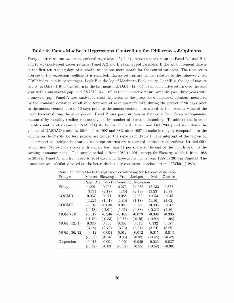
Table 4: Fama-MacBeth Regressions Controlling for Difference-of-Opinions

Every quarter, we run two cross-sectional regressions of (-5,-1) pre-event excess returns (Panel A.1 and B.1)

and (0,+5) post-event excess returns (Panel A.2 and B.2) on lagged variables. If the announcement date is

in the first ten trading days of a month, we lag one more month for the control variables. The time-series

average of the regression coefficients is reported. Excess returns are defined relative to the value-weighted

CRSP index, and in percentages. LogMB is the log of Market-to-Book equity, LogME is the log of market

equity, MOM(−1, 0) is the return in the last month, MOM(−12,−1) is the cumulative return over the past

year with a one-month gap, and MOM(−36,−12) is the cumulative return over the past three years with

a one-year gap. Panel A uses analyst forecast dispersion as the proxy for difference-of-opinions, measured

by the standard deviation of all valid forecasts of next quarter’s EPS during the period of 90 days prior

to the announcement date to 10 days prior to the announcement date, scaled by the absolute value of the

mean forecast during the same period. Panel B uses past turnover as the proxy for difference-of-opinions,

measured by monthly trading volume divided by number of shares outstanding. To address the issue of

double counting of volume for NASDAQ stocks, we follow Anderson and Dyl (2005) and scale down the

volume of NASDAQ stocks by 50% before 1997 and 38% after 1997 to make it roughly comparable to the

volume on the NYSE. Lottery proxies are defined the same as in Table 1. The intercept of the regression

is not reported. Independent variables (except returns) are winsorized at their cross-sectional 1st and 99th

percentiles. We exclude stocks with a price less than $1 per share at the end of the month prior to the

earnings announcements. The sample period is from 1985 to 2014 except for Skewexp which is from 1988

to 2014 in Panel A, and from 1972 to 2014 except for Skewexp which is from 1988 to 2014 in Panel B. The

t-statistics are calculated based on the heteroskedasticity-consistent standard errors of White (1980).

Panel A: Fama-MacBeth regressions controlling for forecast dispersionProxy= Maxret Skewexp Prc Jackpotp Ivol Z-score

Panel A.1: (-5,-1) Pre-event RegressionProxy 4.291 0.263 0.276 24.035 12.133 0.372

(3.77) (2.17) (4.36) (2.79) (3.23) (3.83)LOGMB 0.057 0.071 0.088 0.052 0.053 0.045

(1.22) (1.61) (1.80) (1.18) (1.16) (1.02)LOGME -0.015 -0.038 0.026 0.022 -0.005 0.047

(-0.78) (-2.01) (1.31) (0.88) (-0.23) (2.36)MOM(-1,0) -0.617 -0.246 -0.108 -0.079 -0.309 -0.336

(-1.76) (-0.83) (-0.35) (-0.26) (-0.99) (-1.08)MOM(-12,-1) 0.330 0.336 0.392 0.343 0.332 0.387

(3.18) (2.72) (3.76) (3.21) (3.24) (3.69)MOM(-36,-12) -0.012 -0.004 0.012 -0.012 -0.015 -0.013

(-0.38) (-0.15) (0.36) (-0.38) (-0.48) (-0.42)Dispersion -0.017 -0.001 -0.020 -0.020 -0.023 -0.037

(-0.42) (-0.03) (-0.52) (-0.55) (-0.59) (-0.99)

36

Proxy= Maxret Skewexp Prc Jackpotp Ivol Z-score

Panel A.2: (0,+5) Post-event RegressionProxy -7.874 -0.664 -0.450 -54.701 -28.392 -0.549

(-5.19) (-4.42) (-5.34) (-5.06) (-6.76) (-5.23)LOGMB -0.035 -0.086 -0.071 -0.023 -0.019 -0.014

(-0.62) (-1.45) (-1.21) (-0.43) (-0.34) (-0.25)LOGME 0.013 -0.030 -0.055 -0.070 -0.013 -0.086

(0.52) (-1.09) (-2.10) (-2.35) (-0.57) (-3.44)MOM(-1,0) 0.158 -0.545 -0.803 -0.610 -0.444 -0.373

(0.4) (-1.56) (-2.52) (-1.75) (-1.32) (-1.11)MOM(-12,-1) -0.274 -0.417 -0.398 -0.315 -0.268 -0.321

(-2.30) (-3.30) (-3.40) (-2.70) (-2.35) (-2.77)MOM(-36,-12) -0.033 -0.022 -0.083 -0.039 -0.035 -0.038

(-0.83) (-0.53) (-2.04) (-1.03) (-0.86) (-0.96)Dispersion -0.088 -0.136 -0.058 -0.088 -0.071 -0.044

(-1.59) (-2.30) (-1.06) (-1.60) (-1.30) (-0.81)

Panel B: Fama-MacBeth regressions controlling for past turnoverPanel B.1: (-5,-1) Pre-event Regression

Proxy 1.279 0.317 0.199 6.811 4.078 0.180(2.48) (4.50) (4.32) (3.09) (2.34) (3.53)

LOGMB -0.019 0.000 -0.015 -0.024 -0.019 -0.028(-0.60) (0.01) (-0.49) (-0.79) (-0.62) (-0.93)

LOGME -0.097 -0.042 -0.046 -0.079 -0.091 -0.052(-6.80) (-2.55) (-3.50) (-5.06) (-6.65) (-3.74)

MOM(-1,0) -0.567 -0.458 -0.374 -0.470 -0.487 -0.483(-2.91) (-2.12) (-2.11) (-2.66) (-2.71) (-2.67)

MOM(-12,-1) 0.471 0.245 0.526 0.467 0.474 0.509(6.78) (3.15) (8.11) (6.77) (6.90) (7.66)

MOM(-36,-12) -0.075 -0.046 -0.054 -0.056 -0.073 -0.064(-3.15) (-1.78) (-2.42) (-2.57) (-3.09) (-2.88)

Turnover -1.007 1.960 -0.801 -0.854 -1.059 -1.238(-1.57) (3.55) (-1.28) (-1.32) (-1.64) (-2.05)

Panel B.2: (0,+5) Post-event RegressionProxy -3.386 -0.573 -0.368 -12.369 -10.700 -0.357

(-4.98) (-6.27) (-7.23) (-3.62) (-4.88) (-6.08)LOGMB -0.199 -0.238 -0.195 -0.195 -0.197 -0.171

(-4.93) (-5.25) (-4.80) (-4.67) (-4.84) (-4.37)LOGME 0.044 -0.024 -0.049 0.051 0.037 -0.045

(2.55) (-1.03) (-2.99) (2.58) (2.24) (-2.49)MOM(-1,0) -0.351 -0.571 -0.925 -0.731 -0.627 -0.618

(-1.72) (-2.34) (-5.13) (-3.82) (-3.35) (-3.28)MOM(-12,-1) 0.060 -0.168 -0.024 0.014 0.067 0.021

(0.79) (-1.99) (-0.33) (0.18) (0.90) (0.29)MOM(-36,-12) -0.067 -0.037 -0.119 -0.072 -0.067 -0.085

(-2.15) (-1.21) (-3.91) (-2.32) (-2.18) (-2.84)Turnover -5.171 -3.273 -5.530 -5.381 -5.069 -4.782

(-7.24) (-5.21) (-7.76) (-7.28) (-7.07) (-6.95)

37

Table 5: Evidence from Retail Trade Imbalance

Each quarter, firms with earnings announcements in that quarter are sorted into five portfolios based on

each one of six lottery proxies from the month prior to the announcement date. If the announcement date

is in the first ten trading days of a month, we lag one more month for the proxies. Panel A reports the

change in retail trade imbalance of bottom and top quintile lottery portfolios and their differences in the pre-

event period. We first compute daily retail trade imbalance using the difference between buy-initiated and

sell-initiated small-trade volume divided by the total of buy-initiated and sell-initiated small-trade volume:

RIMB = (BUYVOL − SELLVOL)/(BUYVOL + SELLVOL), where BUYVOL and SELLVOL are the daily

buy- and sell- initiated small-trade volume of this stock, respectively. We then aggregate the daily retail

trade imbalance during (-10,-6) and (-5,-1) event windows, with day 0 referring to the earnings announcement

date. The pre-event change is the (-5,-1) RIMB minus (-10,-6) RIMB, normalized by the absolute value of the

(-5,-1) RIMB. Panel B reports the time-series average of the regression coefficients from the Fama-MacBeth

predictive regressions. We add two independent variables: (-5,-1) RIMB and its interaction with our lottery

proxies into the Fama-MacBeth regressions in Panel B in Table 4. Lottery proxies are defined the same

as in Table 1. We only include NYSE and AMEX common stocks, and require the price to be at least

$1 at the end of month prior to the earnings announcements. Independent variables (except returns) are

winsorized at their cross-sectional 1st and 99th percentiles. The sample period is from 1983 to 2000 except

for Skewexp which is from 1988 to 2000. The t-statistics are calculated based on the heteroskedasticity-

adjusted standard errors of Newey-West (1987) in Panel A, and the heteroskedasticity-consistent standard

errors of White (1980) in Panel B. We only report the bottom and top quintile lottery portfolios and their

differences in Panel A, and the regression coefficients of RIMB, lottery proxies, and the interaction terms in

Panel B, to save space.

Proxy= Maxret Skewexp Prc Jackpotp Ivol Z-score

Panel A: (-5,-1) Pre-event change in RIMB of lottery portfoliosQ1 0.213 -0.030 0.084 0.175 0.177 0.133Q5 0.242 0.285 0.377 0.285 0.235 0.316Q5-Q1 0.029 0.314 0.294 0.110 0.059 0.182t-stat (1.31) (6.85) (2.91) (2.03) (2.04) (4.22)

Panel B: (-5,-1) Pre-event Fama-MacBeth regressionsRIMB 0.412 0.220 2.598 0.357 0.148 1.166

(12.97) (5.30) (23.86) (11.08) (4.21) (24.63)Proxy 4.855 1.021 0.531 48.533 20.718 0.581

(4.89) (7.19) (7.6) (7.72) (5.57) (7.00)Proxy x RIMB 8.840 1.012 0.613 52.743 35.006 0.713

(14.97) (16.18) (19.97) (16.46) (17.75) (17.51)CONTROLS YES YES YES YES YES YES

38

Table 6: Fama-MacBeth Regressions with Religious Beliefs Interactions

Each quarter, we run two sets of cross-sectional regressions of (-5,-1) pre-event excess returns (Panel A)

and (0,+5) post-event excess returns (Panel B) on lagged variables. If the announcement date is in the

first ten trading days of a month, we lag one more month for the control variables. The time-series average

of the regression coefficients is reported. Excess returns are defined relative to the value-weighted CRSP

index, and in percentages. LogCPRATIO is the log of Catholic-Protestant ratio from Kumar et al. (2011).

LogMB is the log of Market-to-Book equity, LogME is the log of market equity, MOM(−1, 0) is the return

in the last month, MOM(−12,−1) is the cumulative return over the past year with a one-month gap, and

MOM(−36,−12) is the cumulative return over the past three years with a one-year gap. Lottery proxies are

defined the same as in Table 1. Independent variables (except returns) are winsorized at their cross-sectional

1st and 99th percentiles. We exclude stocks with a price less than $1 per share at the end of the month prior

to the earnings announcements. The sample period is from 1972 to 2010 except for Skewexp which is from

1988 to 2010. The t-statistics are calculated based on the heteroskedasticity-consistent standard errors of

White (1980).

Proxy= Maxret Skewexp Prc Jackpotp Ivol Z-score

Panel A: (-5,-1) Pre-event RegressionLOGCPRATIO -0.001 0.010 0.104 0.002 -0.020 0.034

(-0.07) (0.50) (2.06) (0.11) (-0.84) (2.69)Proxy 1.967 0.400 0.245 8.329 6.434 0.247

(3.49) (5.00) (4.79) (3.56) (3.54) (4.74)Proxy x LOGCPRATIO 0.722 0.052 0.026 1.785 2.709 0.032

(2.16) (1.95) (1.61) (1.32) (2.41) (2.08)LOGMB -0.020 0.000 -0.014 -0.024 -0.023 -0.032

(-0.59) (0.01) (-0.4) (-0.70) (-0.66) (-0.95)LOGME -0.101 -0.040 -0.039 -0.081 -0.091 -0.037

(-6.43) (-2.09) (-2.4) (-4.72) (-6.01) (-2.43)MOM(-1,0) 0.058 -0.328 0.337 0.213 0.180 0.176

(0.24) (-1.27) (1.54) (0.97) (0.8) (0.79)MOM(-12,-1) 0.521 0.290 0.577 0.509 0.527 0.556

(6.21) (3.12) (7.37) (6.31) (6.3) (6.87)MOM(-36,-12) -0.075 -0.059 -0.048 -0.058 -0.068 -0.059

(-3.06) (-1.98) (-2.02) (-2.57) (-2.84) (-2.55)Turnover -1.838 2.078 -1.246 -1.324 -1.847 -1.996

(-2.32) (3.35) (-1.64) (-1.65) (-2.26) (-2.59)

Panel B: (0,+5) Post-event RegressionLOGCPRATIO -0.006 0.058 -0.150 -0.010 0.005 -0.021

(-0.28) (1.85) (-2.62) (-0.47) (0.19) (-1.39)Proxy -3.452 -0.504 -0.329 -7.737 -10.384 -0.362

(-4.68) (-4.88) (-5.87) (-2.10) (-4.55) (-5.94)Proxy x LOGCPRATIO -0.458 -0.123 -0.049 -1.612 -1.643 -0.043

(-1.14) (-3.01) (-2.67) (-1.10) (-1.29) (-2.30)LOGMB -0.200 -0.247 -0.197 -0.211 -0.194 -0.165

(-4.40) (-4.80) (-4.33) (-4.53) (-4.24) (-3.77)LOGME 0.042 -0.025 -0.043 0.061 0.038 -0.055

(2.11) (-0.97) (-2.36) (2.80) (2.07) (-2.78)MOM(-1,0) -0.713 -0.724 -1.290 -1.128 -1.010 -0.979

(-2.75) (-2.52) (-5.53) (-4.71) (-4.17) (-4.03)MOM(-12,-1) 0.027 -0.225 -0.048 0.006 0.023 -0.023

(0.33) (-2.36) (-0.59) (0.07) (0.29) (-0.28)MOM(-36,-12) -0.099 -0.066 -0.142 -0.104 -0.102 -0.119

(-2.68) (-2.05) (-3.85) (-2.73) (-2.74) (-3.26)Turnover -5.170 -3.569 -5.781 -5.641 -5.048 -4.668

(-5.96) (-4.97) (-6.69) (-6.49) (-5.88) (-5.60)

39

Table 7: Pre-event and Post-event Portfolio Returns among Bottom and Top50% IO Subsample

Each quarter, firms with earnings announcements are first divided into 2 groups based on the institutional

ownership (IO). Within each IO group, firms are further sorted into five portfolios based on each one of

six lottery proxies from the month prior to the announcement date. If the announcement date is in the

first ten trading days of a month, we lag one more month for the proxies. We report equal-weighted excess

returns of these lottery portfolios, and the differences between top and bottom quintile portfolios during the

(-5,-1) pre-event period in Panel A.1 and the (0,+5) post-event period in Panel B.1, with day 0 referring to

the earnings announcement date. IO is calculated as the percentage of firms’ shares held by institutional

investors at the end of prior quarter. Lottery proxies are defined the same as in Table 1. We exclude stocks

with a price less than $1 per share at the end of the month prior to the earnings announcements. The sample

period is from 1980 to 2014 except for Skewexp which is from 1988 to 2014. Excess returns are reported

in percentages. The t-statistics are calculated based on the heteroskedasticity-consistent standard errors of

White (1980). We only report the bottom and top quintile lottery portfolios and their differences to save

space.

Panel A: (-5,-1) Pre-event Excess ReturnProxy= Maxret Skewexp Prc Jackpotp Ivol Z-score

Panel A.1: Bottom 50% IO subsampleQ1 0.117 0.176 0.141 0.169 0.145 0.118Q5 0.520 0.727 0.752 0.727 0.575 0.624Q5-Q1 0.403 0.551 0.611 0.558 0.430 0.506t-stat (3.45) (4.07) (4.62) (4.23) (3.28) (3.72)

Panel A.2: Top 50% IO subsampleQ1 0.025 0.257 0.158 0.068 0.050 0.042Q5 0.337 0.301 0.227 0.291 0.342 0.316Q5-Q1 0.312 0.044 0.069 0.223 0.291 0.274t-stat (2.66) (0.35) (0.67) (1.74) (2.24) (1.98)

Panel A.3: Top minus Bottom 50% IO subsampleQ5-Q1 -0.091 -0.508 -0.542 -0.335 -0.138 -0.232t-stat (-1.04) (-4.07) (-4.93) (-3.13) (-1.45) (-2.22)

Panel B: (0,+5) Post-event Excess ReturnPanel B.1: Bottom 50% IO subsample

Q1 0.227 -0.054 -0.003 0.043 0.197 0.195Q5 -0.801 -0.486 -0.369 -0.489 -0.719 -0.654Q5-Q1 -1.028 -0.432 -0.367 -0.532 -0.916 -0.849t-stat (-6.81) (-2.64) (-2.40) (-3.20) (-5.64) (-4.97)

Panel B.2: Top 50% IO subsampleQ1 0.239 0.245 0.223 0.211 0.285 0.294Q5 -0.122 0.062 0.017 0.035 -0.142 -0.151Q5-Q1 -0.361 -0.183 -0.206 -0.176 -0.427 -0.446t-stat (-2.58) (-1.10) (-1.42) (-1.11) (-2.61) (-2.55)

Panel B.3: Top minus Bottom 50% IO subsampleQ5-Q1 0.666 0.249 0.160 0.356 0.488 0.404t-stat (5.91) (1.68) (1.03) (2.37) (3.81) (2.88)

40

Table 8: Pre-event and Post-event Portfolio Returns for Non-US G7 Countries

This table reports the pre-event and post-event portfolio returns for non-US G7 countries. Each quarter

in each country, firms with earnings announcements are divided into five portfolios based on a composite

z-score of three lottery proxies (Maxret, Prc, and Ivol) from the month prior to the announcement date. If

the announcement date is in the first ten trading days of a month, we lag one more month for the proxies.

Maxret is the maximum daily return, Prc is negative log of one plus stock price, i.e., Prc = −log(1 + Price),

and Ivol is idiosyncratic volatility from Ang, Hodrick, Xing, and Zhang (2009). We report equal-weighted

excess returns of these z-score portfolios, and the differences between top and bottom quintile portfolios

during the (-5,-1) pre-event period in Panel A and the (0,+5) post-event period in Panel B, with day 0

referring to the earnings announcement date. Detailed variable definitions are described in the Appendix.

The sample period is from September 1999 to December 2014 for Canada, April 2002 to December 2014 for

Germany, January 2004 to September 2014 for France, January 1994 to December 2014 for UK, April 2003

to December 2014 for Italy, and October 2001 to December 2014 for Japan. Excess returns are reported

in percentages. The t-statistics are calculated based on the heteroskedasticity-consistent standard errors of

White (1980).

Country Canada Germany France UK Italy Japan

Panel A: (-5,-1) Pre-event Excess ReturnQ1 -0.037 0.073 0.356 0.502 0.420 0.217Q2 -0.063 0.383 0.092 0.552 0.056 0.039Q3 0.339 0.492 0.147 0.580 -0.010 0.037Q4 0.173 0.617 0.652 0.724 0.198 0.149Q5 0.622 1.270 0.867 0.776 -0.040 0.239Q5-Q1 0.659 1.197 0.511 0.274 -0.460 0.022t-stat (2.16) (3.58) (1.85) (1.39) (-2.03) (0.12)

Panel B: (0,+5) Post-event Excess ReturnQ1 0.295 0.172 -0.043 1.299 0.043 0.056Q2 -0.217 -0.353 0.445 1.373 -0.220 -0.070Q3 -0.446 -0.006 0.638 1.229 -0.154 -0.224Q4 -0.410 -0.678 0.446 0.771 -0.505 -0.341Q5 -0.281 -0.759 -0.705 -0.365 -0.897 -1.105Q5-Q1 -0.576 -0.931 -0.662 -1.664 -0.941 -1.162t-stat (-2.05) (-2.3) (-1.66) (-6.98) (-2.90) (-4.82)

41

Table 9: Realized Skewness of Event Returns and Earnings Surprises

Each quarter, firms with earnings announcements in that quarter are sorted into five portfolios based on each

one of six lottery proxies from the month prior to the announcement date. If the announcement date is in the

first ten trading days of a month, we lag one more month for the proxies. We report the skewness (Panel A.1)

of firm-quarter panel excess returns during the (-1,+1) 3-day event-window centered at the announcement

date for the top and bottom quintile portfolios, and their differences. We also present analogous skewness

(Panel A.2) using pseudo-announcement dates. Pseudo-announcement dates are computed by subtracting a

randomly selected number of trading days from the actual announcement date, where the random numbers

are drawn from a uniform distribution spanning 10 to 40 days. Panel A.3 compares the differences between

actual- and pseudo-announcement dates. Panel B reports the skewness of firm-quarter panel earnings surprise

at the announcement date for the top and bottom quintile portfolios, and their differences. The earnings

surprise is calculated by taking the difference between actual quarterly earnings per share and the most

recent median consensus EPS forecast of analysts for that quarter normalized by assets per share at previous

quarter end. Lottery proxies are defined the same as in Table 1. We exclude stocks with a price less than

$1 per share at the end of the month prior to the earnings announcements. The sample period is from 1972

to 2014 in Panel A, from 1985 to 2014 in Panel B, and from 1988 to 2014 for Skewexp in both panels. We

only report the bottom and top quintile lottery portfolios and their differences to save space.

Proxy= Maxret Skewexp Prc Jackpotp Ivol Z-scorePanel A: skewness of (-1,+1) Excess Return

Panel A.1: Actual datesQ1 1.468 0.278 0.079 0.203 0.645 0.118Q5 3.601 4.156 4.011 3.981 3.732 3.890Q5-Q1 2.134 3.878 3.932 3.778 3.087 3.772

Panel A.2: Pseudo datesQ1 1.263 0.177 -0.445 0.832 0.747 0.681Q5 1.583 -0.680 2.267 1.694 1.492 0.973Q5-Q1 0.320 -0.857 2.712 0.862 0.745 0.292

Panel A.3: Actual dates minus Pseudo datesQ1 0.205 0.101 0.524 -0.628 -0.102 -0.563Q5 2.018 4.836 1.744 2.287 2.240 2.917Q5-Q1 1.813 4.735 1.220 2.916 2.343 3.480

Panel B: Skewness of earnings surpriseQ1 -3.900 -2.651 -1.419 -4.363 -4.234 -3.874Q5 -1.342 -1.146 -1.107 -1.159 -1.213 -1.083Q5-Q1 2.559 1.506 0.312 3.204 3.021 2.791

42

Table 10: Pre-event and Post-event Portfolio Returns among Early/On-time/Late Announcers

Each quarter, firms with earnings announcements in that quarter are sorted into five portfolios based on each

one of six lottery proxies from the month prior to the announcement date. If the announcement date is in the

first ten trading days of a month, we lag one more month for the proxies. We report equal-weighted excess

returns of these lottery portfolios and the differences between top and bottom quintile portfolios during the

(-5,-1) pre-event period in Panel A and the (0,+5) post-event period in Panel B within the subsample of

early, on-time, and late announcers relative to the expected earnings announcement dates. Expected earnings

announcement dates are calculated by adding the historical reporting lag to the current fiscal quarter end.

The historical reporting lag is the median number of trading days between a firm’s fiscal quarter end and

its actual announcement dates for the same fiscal quarter over the previous ten years. Early, on-time, and

late announcers are firms whose actual announcement dates are more than one day before, within one day,

and more than one day after the expected earnings announcement dates, respectively. Lottery proxies are

defined the same as in Table 1. We exclude stocks with a price less than $1 per share at the end of the month

prior to the earnings announcements. The sample period is from 1972 to 2014 except for Skewexp which is

from 1988 to 2014. Excess returns are reported in percentages. The t-statistics are calculated based on the

heteroskedasticity-consistent standard errors of White (1980).

Panel A: (-5,-1) Pre-event Excess ReturnProxy= Maxret Skewexp Prc Jackpotp Ivol Z-score

Panel A.1: Early announcersQ1 0.183 0.309 0.263 0.185 0.164 0.129Q5 1.043 1.182 1.347 1.405 1.089 1.324Q5-Q1 0.860 0.873 1.084 1.220 0.926 1.195t-stat (7.18) (6.31) (10.36) (8.65) (6.90) (8.95)

Panel A.2: On-time announcersQ1 0.152 0.189 0.204 0.098 0.112 0.085Q5 0.452 0.610 0.715 0.606 0.509 0.573Q5-Q1 0.299 0.421 0.510 0.508 0.398 0.488t-stat (2.36) (3.12) (4.09) (3.73) (2.86) (3.53)

Panel A.3: Late announcersQ1 0.008 0.148 0.073 0.027 0.018 0.004Q5 -0.006 0.242 0.138 0.093 0.063 0.031Q5-Q1 -0.013 0.093 0.065 0.066 0.045 0.028t-stat (-0.12) (0.70) (0.51) (0.52) (0.37) (0.20)

Panel B: (0,+5) Post-event Excess ReturnPanel B.1: Early announcers

Q1 0.523 0.329 0.320 0.344 0.479 0.379Q5 0.092 0.370 0.553 0.506 0.193 0.318Q5-Q1 -0.432 0.041 0.233 0.163 -0.286 -0.061t-stat (-3.11) (0.21) (1.52) (1.04) (-1.87) (-0.39)

Panel B.2: On-time announcersQ1 0.266 0.144 0.153 0.181 0.294 0.253Q5 -0.632 -0.534 -0.258 -0.466 -0.486 -0.566Q5-Q1 -0.899 -0.677 -0.411 -0.647 -0.780 -0.818t-stat (-6.57) (-3.74) (-2.93) (-4.08) (-5.35) (-5.46)

Panel B.3: Late announcersQ1 0.020 0.035 0.103 0.058 0.082 0.137Q5 -0.972 -0.969 -0.648 -0.935 -0.984 -0.882Q5-Q1 -0.992 -1.004 -0.752 -0.993 -1.066 -1.020t-stat (-6.89) (-5.47) (-4.32) (-6.28) (-6.81) (-5.31)

43

Table 11: Enhanced Lottery Strategy

This table compares the monthly return spreads of the standard lottery strategy (Panel A), our refined

lottery strategy (Panel B), and their differences (Panel C). The standard lottery strategy is constructed by

holding a hedge portfolio from longing bottom quintile lottery portfolios and shorting top quintile lottery

portfolios. Each month, stocks are divided into 5 portfolios based on each one of six lottery proxies from

the previous month. Our refined lottery strategy adds a pre-event strategy to the standard lottery strategy.

Firms with earnings announcements in a certain month are bought if they belong to the top quintile lottery

portfolios and sold if they belong to bottom quintile lottery portfolios during the (-10,-1) pre-event window.

To ensure that the strategy is implementable, we only use the pre-event days after the portfolio formation

date. The portfolio is held for one month and value-weighted excess return and Fama-French four-factor

alpha spreads are calculated. Lottery proxies are defined the same as in Table 1. We exclude stocks with

price less than $1 at the end of the previous month. The sample period is from 1972 to 2014 except for

Skewexp which is from 1988 to 2014. Excess returns and FF4 alphas are reported in percentages. The

t-statistics are calculated based on the heteroskedasticity-consistent standard errors of White (1980). We

only report the bottom and top quintile lottery portfolios and their differences to save space.

Proxy= Maxret Skewexp Prc Jackpotp Ivol Z-score

Panel A: Standard lottery strategyQ1 0.577 0.790 0.522 0.547 0.568 0.583Q5 0.145 0.211 0.523 -0.186 -0.244 -0.449Re

Q1−Q5 0.432 0.579 -0.001 0.733 0.811 1.031

t-stat (1.59) (1.61) (0.00) (2.10) (2.76) (2.99)αFF4Q1−Q5 0.514 0.412 -0.006 0.835 0.881 1.085

t-stat (2.95) (1.82) (-0.03) (4.36) (4.85) (5.01)

Panel B: Refined lottery strategyQ1 0.359 0.460 0.256 0.271 0.299 0.322Q5 -0.236 -0.277 -0.165 -0.729 -0.586 -0.910Re

Q1−Q5 0.595 0.737 0.421 1.000 0.885 1.231

t-stat (2.58) (2.54) (1.5) (3.45) (3.55) (4.22)αFF4Q1−Q5 0.810 0.795 0.597 1.288 1.144 1.500

t-stat (4.16) (3.37) (2.53) (6.55) (6.31) (7.30)

Panel C: Refined strategy minus standard strategyQ1 -0.218 -0.329 -0.266 -0.276 -0.269 -0.261Q5 -0.381 -0.488 -0.689 -0.543 -0.342 -0.461Re

Q1−Q5 0.163 0.158 0.422 0.267 0.073 0.200

t-stat (1.23) (0.94) (3.20) (1.71) (0.55) (1.46)αFF4Q1−Q5 0.295 0.382 0.603 0.453 0.263 0.415

t-stat (1.79) (2.10) (3.71) (2.45) (1.61) (2.48)

44

Appendix: Definitions of Key Variables

This appendix provides the details for constructing the lottery measures.

Skewexp: The expected idiosyncratic skewness is calculated in two steps following Boyer,

Mitton, and Vorkink (2010) (Table 2, Model 6, page 179). First, we estimate the following

cross-sectional regressions separately at the end of each month t:

isi,t = β0,t + β1,tisi,t−60 + β2,tivi,t−60 + λ′

tXi,t−60 + εi,t,

where isi,t and ivi,t denote the historical estimates of idiosyncratic volatility and skewness

relative to the Fama and French three-factor model, respectively, for firm i using daily

stock data over the past 60 months till month t. Xi,t is a set of firm-specific variables

including momentum as the cumulative returns over months t− 72 through t− 61, turnover

as the average daily turnover in month t− 60, the small-size market capitalization dummy,

the medium-size market capitalization dummy, the industry dummy based on the Fama-

French 17-industries definition, and the NASDAQ dummy. After we have these regression

parameters, the expected idiosyncratic skewness for each firm i at the end of each month t

is then computed in the second step:

Skewexpt ≡ Et[isi,t+60] = β0,t + β1,tisi,t + β2,tivi,t + λ′

tXi,t.

Similar to Boyer, Mitton, and Vorkink’s (2010) baseline database, our expected idiosyncratic

skewness measure dates back to January 1988.

Jackpotp: The predicted jackpot probability is constructed from the baseline model in

Conrad, Kapadia, and Xing (2014) (Table 3, Panel A, page 461). In particular, for each

firm, we first estimate the baseline logit model using data from the past 20 years at the end

of June every year:

Probt−1(Jackpoti,t = 1) =exp(a+ b×Xi,t−1)

1 + exp(a+ b×Xi,t−1),

where Jackpoti,t is a dummy that equals 1 if firm i’s log return in the next 12 month period

is larger than 100%. The vector Xi,t−1 is a set of firm-specific variables known at time t− 1,

including skewness of log daily returns (centered around 0) over the last 3 months, log stock

return over the past year, firm age as the number of years since appearance on CRSP, asset

tangibility as the ratio of gross PPE (property plant and equipment) to total assets, the log

45

of sales growth over the prior year, detrended stock turnover as the difference between the

average past 6-month turnover and the average past 18-month turnover, volatility as the

standard deviation of daily returns (centered around 0) over the past 3 months, and the log

of market equity in thousands. Next, we use these estimated parameters to construct the

out-of-sample predicted jackpot probability (Jackpotp). We reestimate this model for each

firm every year from 1951, so our first set of out-of-sample predicted jackpot probabilities is

from January 1972.

Ivol : The idiosyncratic stock return volatility is constructed following Ang, Hodrick,

Xing, and Zhang (2006). In particular, we measure IVOL by the standard deviation of the

residual values from the following time-series model:

Ri,t = b0 + b1RM,t + b2SMBt + b3HMLt + εi,t, (1)

where Ri,t is stock i’s daily excess return on date t, and RM,t, SMBt, and HMLt are the

market factor, size factor, and value factor on date t, respectively.18 We estimate the above

equation for each stock each month in the data set using the daily return from the previous

month with a minimum requirement of 10 nonmissing values.19

Z-score: Z-score is a monthly composite lottery measure calculated as the average of the

individual z-scores of the following five lottery measures: Maxret, Skewexp, Prc, Jackpotp,

and Ivol. Each month for each stock, each one of the five lottery measures is first converted

into its rank and then standardized to obtain its z-score: z = (r − µr)/σr, where r is the

rank of this measure, µr and σr are the cross sectional mean and standard deviation of r.

The composite z-score is the average of these five z-scores. We require a minimum of three

nonmissing z-scores to compute this measure.

Non-US G7 countries: Following Gao et al (2015), for each country, we only include

common stocks traded on its major national stock exchanges. Most countries have only one

major exchange except for Canada, for which we use stocks from both the Toronto Stock

Exchange and the TSX Ventures Exchange, and Japan, for which we include all stocks traded

on the Osaka Securities Exchange, the Tokyo Stock Exchange, and JASDAQ. We convert

all returns, prices, and accounting variables from local currency to US dollars. We further

exclude micro-cap firms which have market equity below 5% in each quarter in a country.

Returns are winsorized at 0.5 and 99.5 percentiles to avoid extreme values.

18We thank Ken French for providing updated series for these factors.19Our results are not sensitive to this cutoff.

46

To measure the lottery feature of international stocks, we use three proxies similar to

our definitions for US stocks: Maxret is the maximum daily return within a month, and

Prc is negative log of one plus month-end stock price, i.e., Prc = −log(1 + Price)). To

compute Ivol for each country, we first specify a local version of the Fama-French three-

factor model including a local market excess return factor, a local size factor, and a local

value factor, following Ang et al. (2009) and Gao et al. (2015). The market factor is

the value-weighted return of the local market portfolio minus the one-month U.S. T-bill

rate. The country-specific size is the return spread between the smallest and biggest local

firms, and the value factor is the spread between the local value and growth firms. The

idiosyncratic volatility (Ivol) is computed as the standard idiosyncratic volatility measure,

i.e., the standard deviation of residuals from the daily local factor model within a month

with a minimum requirement of 10 nonmissing values. After we obtain Maxret, Prc, and Ivol

for each stock, we construct a composite z-score as the average of these individual z-scores.

Further, to ensure the accuracy of earnings announcement dates for international

countries, we only use dates that can be confirmed from multiple available data sources.

In particular, we require the dates to exist in both Thomson Reuters Worldscope database

and Bloomberg for non-US G7 countries except for Canada, for which we require the dates

to exist in all three data sources: Thomson Reuters Worldscope database, Compustat North

American database and Bloomberg. Lastly, we require a minimum of 50 stocks when forming

portfolios to avoid the potential bias from having portfolios with too few assets.

47