TIME VARIATION OF KEPLER TRANSITS INDUCED BY STELLAR ROTATING SPOTS—A WAY TODISTINGUISH BETWEEN PROGRADE AND RETROGRADE MOTION. I. THEORY

Tsevi Mazeh1,2, Tomer Holczer1, and Avi Shporer3,4,51 School of Physics and Astronomy, Raymond and Beverly Sackler Faculty of Exact Sciences,

Tel Aviv University, Tel Aviv 69978, Israel; mazeh@post.tau.ac.il2 The Jesus Serra Foundation Guest Program, Instituto de Astrofsica de Canarias, C. via Lactea S/N, E-38205 La Laguna, Tenerife, Spain

3 Division of Geological and Planetary Sciences, California Institute of Technology, Pasadena, CA 91125, USA4 Jet Propulsion Laboratory, California Institute of Technology, 4800 Oak Grove Drive, Pasadena, CA 91109, USA

Received 2014 June 23; accepted 2014 December 30; published 2015 February 20

ABSTRACT

Some transiting planets discovered by the Kepler mission display transit timing variations (TTVs) induced bystellar spots that rotate on the visible hemisphere of their parent stars. An induced TTV can be observed when aplanet crosses a spot and modifies the shape of the transit light curve, even if the time resolution of the data doesnot allow the detection of the crossing event itself. We present an approach that can, in some cases, use the derivedTTVs of a planet to distinguish between a prograde and a retrograde planetary motion with respect to the stellarrotation. Assuming a single spot darker than the stellar disk, spot crossing by the planet can induce measuredpositive (negative) TTV, if the crossing occurs in the first (second) half of the transit. On the other hand, themotion of the spot toward (away from) the center of the stellar visible disk causes the stellar brightness to decrease(increase). Therefore, for a planet with prograde motion, the induced TTV is positive when the local slope of thestellar flux at the time of transit is negative, and vice versa. Thus, we can expect to observe a negative (positive)correlation between the TTVs and the photometric slopes for prograde (retrograde) motion. Using a simplisticanalytical approximation, and also the publicly available SOAP-T tool to produce light curves of transits with spot-crossing events, we show for some cases how the induced TTVs depend on the local stellar photometric slopes atthe transit timings. Detecting this correlation in Kepler transiting systems with high enough signal-to-noise ratiocan allow us to distinguish between prograde and retrograde planetary motions. In upcoming papers we presentanalyses of the KOIs and Kepler eclipsing binaries, following the formalism developed here.

Key words: planetary systems – starspots – stars: rotation – techniques: photometric

1. INTRODUCTION

Formation and evolutionary processes of stellar andplanetary systems are expected to leave their imprint on thepresent-day systems. One such imprint is the stellar obliquity,the angle between the stellar spin axis and the orbital angularmomentum axis, also referred to as the spin–orbit angle. Forstar–planet systems the measurement of this angle is a matter ofintense study in recent years (e.g., Triaud et al. 2010; Moutouet al. 2011; Winn et al. 2011; Albrecht et al. 2012), primarilyfor hot Jupiters—gas-giant planets at short-period orbits. Someof the systems were found to be aligned, in a prograde orbitwith the spin–orbit angle close to zero, while others were foundto be misaligned, including systems in retrograde motion wherethe spin–orbit angle is close to 180° (e.g., Hébrard et al. 2011;Winn et al. 2011).

The growing sample and the wide range of spin–orbit anglesmeasured for hot Jupiters can be used for studying their orbitalevolutionary history. For example, Winn et al. (2010) havenoticed that hot stars, with an effective temperature above6250 K, tend to have a wide obliquity range, while cool starstend to have low obliquities, mostly consistent with well-aligned orbits. This was confirmed by a study of a largersample by Albrecht et al. (2012) and is consistent with theresults of Schlaufman (2010) and Hansen (2012) who useddifferent approaches. Those authors suggested that somemechanisms can cause the planetary orbit to attain largeobliquity (e.g., Fabrycky & Tremaine 2007; Naoz et al. 2011;

Batygin 2012). Then, tidal interaction with the host star (e.g.,Winn et al. 2010) or magnetic braking (e.g., Dawson 2014)acts to realign the orbit. Since these processes are probablyinefficient for hot stars, those systems might still retain theirwide obliquity range.So far spin–orbit alignment has been studied primarily

through the Rossiter–McLaughlin (RM) effect (Holt 1893;Schlesinger 1910; Rossiter 1924; McLaughlin 1924), originallysuggested for stellar eclipsing binaries, and observed bymonitoring the anomalous radial-velocity signal during eclipse,as the eclipsing star moves across the disk of the eclipsed star.The RM effect is sensitive to the sky-projected component ofthe spin–orbit angle, and was successfully measured for manytransiting planet systems (e.g., Queloz et al. 2000; Winnet al. 2006; Triaud et al. 2010), transiting brown dwarfs, andlow-mass star systems (Triaud et al. 2013), and stellar binaries(Albrecht et al. 2007, 2009, 2011, 2014).The line-of-sight component of the spin–orbit angle can be

measured using asteroseismology (Gizon & Solanki 2003;Chaplin et al. 2013), or the observed rotational broadening ofspectral lines, if the host star radius and rotation period areknown with sufficient precision (Hirano et al. 2012, 2014; seealso Schlaufman 2010). However, these two methods requireobtaining new data for each target, using valuable resources(e.g., large telescopes or Kepler short-cadence data). Othermethods have been presented, based on stellar gravitationaldarkening (Barnes 2009; Barnes et al. 2011; Szabo 2011) andthe beaming effect (Photometric RM—Groot 2012; Shporeret al. 2012).

The Astrophysical Journal, 800:142 (12pp), 2015 February 20 doi:10.1088/0004-637X/800/2/142© 2015. The American Astronomical Society. All rights reserved.

5 Sagan Fellow.

1

An interesting approach was taken by Nutzman et al. (2011)and Sanchis-Ojeda et al. (2011), who use the brief photometricsignals during transit induced by the transiting object movingacross spots located on the surface of the host object. This isbased on the fact that many stars show photometric modula-tions resulting from the combination of stellar rotation and non-uniform longitudinal spots distribution (e.g., Irwin et al. 2009;Hartman et al. 2011; McQuillan et al. 2014). When such a stardisplays transits by an orbiting planet, the transiting objectmight momentarily eclipse a stellar spot, inducing an increasein observed flux, if the surface brightness of the spot-coveredarea is lower than that of the non-spotted areas. The derivationof the stellar obliquity requires identification of such “spot-crossing” events within a few transits, and estimate the spot andthe planet phases within their motion over the stellar disk. Themethod has since been applied to additional systems usinghigh-speed Kepler and CoRoT data (Deming et al. 2011;Désert et al. 2011; Sanchis-Ojeda & Winn 2011; Sanchis-Ojedaet al. 2012, 2013).

We present here another version of this approach that doesnot require such high-speed photometry. Instead, we use thefact that a spot-crossing event can induce measurable transittime variation (TTV; e.g., Sanchis-Ojeda et al. 2011; Fabryckyet al. 2012; Mazeh et al. 2013; Szabó et al. 2013; Oshaghet al. 2013b), even for data that cannot resolve the event itself.Our approach relies on the expected correlation between theinduced TTV and the corresponding local photometric slopeimmediately outside the transit, presumably induced by thesame spot. Detected correlation or anti-correlation between theTTVs and their local slope can in principle differentiatebetween prograde and retrograde rotation of the primary star instellar binaries or star–planet systems.

We present here the basic concept and develop an analyticalsimplistic approximation for the induced TTVs and thephotometric slope. We also use the work of Boisse et al.(2012) and Oshagh et al. (2013a), who developed a numericaltool, SOAP-T6, to simulate a planetary transit light curve whichincludes a spot-crossing event. Oshagh et al. (2013b) usedSOAP-T to derive detailed transit light curves, and then fittedthem with transit templates to obtain the expected TTVs, verysimilar to what is performed when deriving the TTVs from theKepler actual data (e.g., Mazeh et al. 2013). We show that ourapproximation yields TTVs with the same order of magnitudeas the results of Oshagh et al. (2013b). Using our approxima-tion and the SOAP-T tool we show that in some cases we canexpect a negative (positive) correlation between the TTVsinduced by spot crossing and the local photometric slopes at thetransit timings for prograde (retrograde) motion of the planet.We also discuss the limitations of this approach when appliedto real data, showing that it can be applied only to a limitednumber of systems.

The paper is organized as follows. Section 2 outlines thebasics of our approach, while Section 3 presents the analyticalapproximation for the induced TTV for different cases, andSection 4 compares our approximation with numericalsimulations we performed and those of Oshagh et al.(2013b). In Section 5 we derive the expected derivative ofthe stellar brightness at the time of transit, and in Section 6display the expected correlation between the induced TTVs and

the stellar photometric slopes. Finally, Section 7 discusses ourresults and the severe limitations of its applicability to real data.The present paper is the first of three studies. The next study

(T. Holczer et al. 2015, in preparation) presents our analysis forthe Kepler planet candidates (Batalha et al. 2013). In that paperwe show that indeed a few systems do show highly significantcorrelation between their derived TTVs and the local photo-metric derivatives, as predicted by this work. A forthcomingpaper will present our analysis of the Kepler eclipsing stellarbinaries (Slawson et al. 2011).

2. THE PRINCIPLE OF THE APPROACH

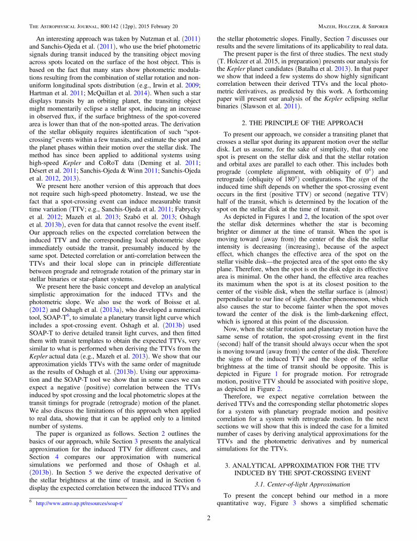
To present our approach, we consider a transiting planet thatcrosses a stellar spot during its apparent motion over the stellardisk. Let us assume, for the sake of simplicity, that only onespot is present on the stellar disk and that the stellar rotationand orbital axes are parallel to each other. This includes bothprograde (complete alignment, with obliquity of 0 ) andretrograde (obliquity of 180°) configurations. The sign of theinduced time shift depends on whether the spot-crossing eventoccurs in the first (positive TTV) or second (negative TTV)half of the transit, which is determined by the location of thespot on the stellar disk at the time of transit.As depicted in Figures 1 and 2, the location of the spot over

the stellar disk determines whether the star is becomingbrighter or dimmer at the time of transit. When the spot ismoving toward (away from) the center of the disk the stellarintensity is decreasing (increasing), because of the aspecteffect, which changes the effective area of the spot on thestellar visible disk—the projected area of the spot onto the skyplane. Therefore, when the spot is on the disk edge its effectivearea is minimal. On the other hand, the effective area reachesits maximum when the spot is at its closest position to thecenter of the visible disk, when the stellar surface is (almost)perpendicular to our line of sight. Another phenomenon, whichalso causes the star to become fainter when the spot movestoward the center of the disk is the limb-darkening effect,which is ignored at this point of the discussion.Now, when the stellar rotation and planetary motion have the

same sense of rotation, the spot-crossing event in the first(second) half of the transit should always occur when the spotis moving toward (away from) the center of the disk. Thereforethe signs of the induced TTV and the slope of the stellarbrightness at the time of transit should be opposite. This isdepicted in Figure 1 for prograde motion. For retrogrademotion, positive TTV should be associated with positive slope,as depicted in Figure 2.Therefore, we expect negative correlation between the

derived TTVs and the corresponding stellar photometric slopesfor a system with planetary prograde motion and positivecorrelation for a system with retrograde motion. In the nextsections we will show that this is indeed the case for a limitednumber of cases by deriving analytical approximations for theTTVs and the photometric derivatives and by numericalsimulations for the TTVs.

3. ANALYTICAL APPROXIMATION FOR THE TTVINDUCED BY THE SPOT-CROSSING EVENT

3.1. Center-of-light Approximation

To present the concept behind our method in a morequantitative way, Figure 3 shows a simplified schematic6 http://www.astro.up.pt/resources/soap-t/

2

The Astrophysical Journal, 800:142 (12pp), 2015 February 20 Mazeh, Holczer, & Shporer

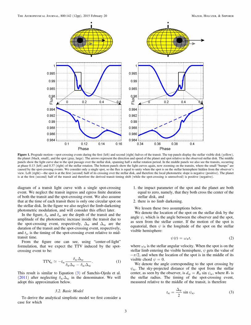
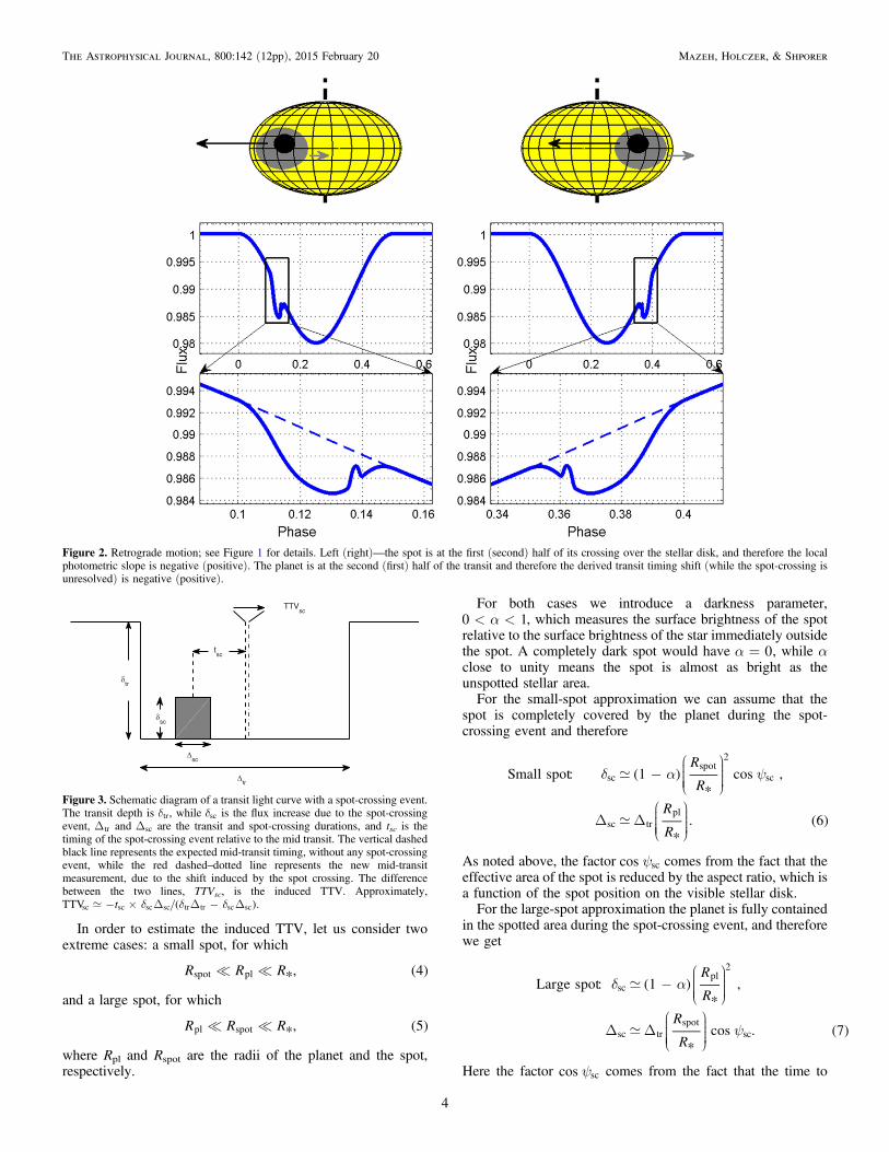
diagram of a transit light curve with a single spot-crossingevent. We neglect the transit ingress and egress finite durationof both the transit and the spot-crossing event. We also assumethat at the time of each transit there is only one circular spot onthe stellar disk. In the figure we also neglect the limb-darkeningphotometric modulation, and will consider this effect later.

In the figure, dtr and dsc are the depth of the transit and theamplitude of the photometric increase inside the transit due tothe spot-crossing event, respectively, Dtr and Dsc are theduration of the transit and the spot-crossing event, respectively,and tsc is the timing of the spot-crossing event relative to mid-transit time.

From the figure one can see, using “center-of-light”formulation, that we expect the TTV induced by the spot-crossing event to be:

dd d

-D

D - D tTTV . (1)sc sc

sc sc

tr tr sc sc

This result is similar to Equation (3) of Sanchis-Ojeda et al.(2011) after neglecting d Dsc sc in the denominator. We willadopt this approximation below.

3.2. Basic Model

To derive the analytical simplistic model we first consider acase for which

1. the impact parameter of the spot and the planet are bothequal to zero, namely, that they both cross the center of thestellar disk, and

2. there is no limb darkening.

We lessen these two assumptions below.We denote the location of the spot on the stellar disk by the

angle ψ, which is the angle between the observer and the spot,as seen from the stellar center. If the motion of the spot isequatorial, then ψ is the longitude of the spot on the stellarvisible hemisphere:

y w=t t( ) * , (2)

where w* is the stellar angular velocity. When the spot is on thestellar limb entering the visible hemisphere, ψ gets the value of-π 2, and when the location of the spot is in the middle of itsvisible chord y = 0.We denote the angle corresponding to the spot crossing by

ysc. The sky-projected distance of the spot from the stellarcenter, as seen by the observer, is y=d R* sinsc sc, where R* isthe stellar radius. The timing of the spot-crossing event,measured relative to the middle of the transit, is therefore

y=D

t2

sin . (3)sctr

sc

Figure 1. Prograde motion—spot-crossing events during the first (left) and second (right) halves of the transit. The top panels display the stellar visible disk (yellow),the planet (black, small), and the spot (gray, large). The arrows represent the direction and speed of the planet and spot relative to the observed stellar disk. The middlepanels show the light curve due to the spot passage over the stellar disk, spanning half a stellar rotation period. In the middle panels we also see the transits, occurringat phase 0.13 (left) and 0.37 (right) of the stellar rotation. The bottom panels show the light curves again, now zooming on the transits, where the small “bumps” arecaused by the spot-crossing events. We consider only a single spot, so the flux is equal to unity when the spot is on the stellar hemisphere hidden from the observer’sview. Left (right)—the spot is at the first (second) half of its crossing over the stellar disk, and therefore the local photometric slope is negative (positive). The planetis at the first (second) half of the transit and therefore the derived transit timing shift (while the spot-crossing is unresolved) is positive (negative).

3

The Astrophysical Journal, 800:142 (12pp), 2015 February 20 Mazeh, Holczer, & Shporer

In order to estimate the induced TTV, let us consider twoextreme cases: a small spot, for which

R R R*, (4)spot pl

and a large spot, for which

R R R*, (5)pl spot

where Rpl and Rspot are the radii of the planet and the spot,respectively.

For both cases we introduce a darkness parameter,a< <0 1, which measures the surface brightness of the spot

relative to the surface brightness of the star immediately outsidethe spot. A completely dark spot would have a = 0, while αclose to unity means the spot is almost as bright as theunspotted stellar area.For the small-spot approximation we can assume that the

spot is completely covered by the planet during the spot-crossing event and therefore

d a y-æ

èçççç

ö

ø÷÷÷÷

D Dæ

èçççç

ö

ø÷÷÷÷

R

R

R

R

Small spot: (1 )*

cos ,

*. (6)

scspot

2

sc

sc trpl

As noted above, the factor ycos sc comes from the fact that theeffective area of the spot is reduced by the aspect ratio, which isa function of the spot position on the visible stellar disk.For the large-spot approximation the planet is fully contained

in the spotted area during the spot-crossing event, and thereforewe get

d a

y

-æ

èçççç

ö

ø÷÷÷÷

D Dæ

èçççç

ö

ø÷÷÷÷

R

R

R

R

Large spot: (1 )*

,

*cos . (7)

scpl

2

sc trspot

sc

Here the factor ycos sc comes from the fact that the time to

Figure 2. Retrograde motion; see Figure 1 for details. Left (right)—the spot is at the first (second) half of its crossing over the stellar disk, and therefore the localphotometric slope is negative (positive). The planet is at the second (first) half of the transit and therefore the derived transit timing shift (while the spot-crossing isunresolved) is negative (positive).

Figure 3. Schematic diagram of a transit light curve with a spot-crossing event.The transit depth is dtr, while dsc is the flux increase due to the spot-crossingevent, Dtr and Dsc are the transit and spot-crossing durations, and tsc is thetiming of the spot-crossing event relative to the mid transit. The vertical dashedblack line represents the expected mid-transit timing, without any spot-crossingevent, while the red dashed–dotted line represents the new mid-transitmeasurement, due to the shift induced by the spot crossing. The differencebetween the two lines, TTVsc, is the induced TTV. Approximately,

d d d- ´ D D - D tTTV ( )sc sc sc sc tr tr sc sc .

4

The Astrophysical Journal, 800:142 (12pp), 2015 February 20 Mazeh, Holczer, & Shporer

cross the spot by the relatively small planet is reduced by thesame aspect ratio.

We now approximate the TTV to be

dd

-DD

tTTV , (8)sc scsc

tr

sc

tr

and the transit depth dtr to be on the order of R R( *)pl2. We

therefore get for the small-spot approximation

a y

a y

- -æ

èçççç

ö

ø÷÷÷÷

æ

èçççç

ö

ø÷÷÷÷

=- -

-

tR

R

R

R

R

R

tR

R R

small spot: TTV (1 )* * *

cos

(1 )*

cos , (9)

sc scspot

2pl pl

2

sc

scspot2

plsc

and for the large-spot approximation

a y- - tR

Rlarge spot: TTV (1 )

*cos . (10)sc sc

spotsc

Note that when R Rspot pl, Equation (9) Equation (10). Toease the discussion we define as:

=

ì

í

ïïïïïï

î

ïïïïïï

R

R R

R

R

*for small spot

*for large spot.

(11)

spot2

pl

spot

Using Equation (3) we get:

a y y- -D

TTV (1 )2

cos sin , (12)sctr

sc sc

which is valid both for the small- and large-spot approxima-tions. The maximum observed TTV induced by the spotcrossing is

a-D { }max TTV

(1 )

4. (13)sc tr

3.3. Models for Limb Darkening, Impact Parameter, andObliquity

3.3.1. Limb Darkening

To include the stellar limb darkening effect in our model, weconsider a quadratic limb-darkening law of

y y= - - - - g g1 (1 cos ) (1 cos )1 22 , where is the

scaled stellar surface brightness and g1 and g2 are the two limb-darkening coefficients, such that + <g g 11 2 .

The induced TTV is proportional to dsc, the increase of thestellar brightness during the spot crossing, which dependslinearly on the stellar surface brightness , which is now a

function of ψ. Therefore we get

a y y

y y

a y

y y

y y y

=- -D

´ - - - -

=- -D

- -

+ +

-

{{ }

}

( )( )

t t

g g

g g t

g g t t

g t t t

TTV (1 )2

cos ( ) sin ( )

1 (1 cos ) (1 cos )

(1 )2

1 sin ( )

2 sin ( ) cos ( )

sin ( ) cos ( ) cos ( ). (14)

sctr

1 22

tr1 2

1 2

22

Note that because of the limb darkening the transit lightcurve does not have a rectangular shape, so our Equation (1)should be modified. Nevertheless, as this analytical approach isaimed only to understand the features of the TTVs as a functionof the spot-crossing phase, we neglect this effect that will affectall phases alike.

3.3.2. Impact Parameter

Another extension of our simplistic model accounts for anon-zero impact parameter, q=b cos . Note that the stellarrotation is, as before, orthogonal to our line of sight. In thisextension of the simplistic model, both planet and spot stillhave the same impact parameter, namely, both move along thesame chord on the stellar disk, a chord that does not go throughthe center of the disk. Therefore, the spot moves at a colatitudeq q=spot , with an impact parameter q=b cosspot spot. In such acase, the angle ψ fulfill the relation

y q f=cos sin cos , (15)

where now ϕ is the longitude of the planet, and f = 0 is whenthe planet crosses the projection of the stellar rotational axis.The range of ψ is now different: q y- ⩽ ∣ ∣ ⩽π π2 2, and thetiming of the spot crossing is

f=D

t2

sin , (16)b

sctr

sc

where Dbtr is the transit duration when ¹b 0. A good

approximation would be qD = D sinbtr tr .

We now separate the discussion for the small and large spotapproximations. For small spot, the duration of the spot-crossing event,Dsc, is still the same as for b = 0, but the transitduration is shorter by a factor of qsin . The flux increasedepends on ycos , as for b = 0. We can therefore write

d a q f

q

-æ

èçççç

ö

ø÷÷÷÷

D Dæ

èçççç

ö

ø÷÷÷÷

R

R

R

R

Small spot: (1 )*

sin cos ,

*

1

sin. (17)b

scspot

2

sc

sc trpl

Combining these expressions we get

a f f- -D

small spot: TTV (1 )2

cos sin . (18)b

sctr

sc sc

For the large spot case, the duration of the spot-crossingevent,Dsc, is now different, as the planet is crossing a spot thatforms an ellipse on the stellar disk, whose axes are Rspot and

yR cosspot . One can show that the length of the planet’s path

5

The Astrophysical Journal, 800:142 (12pp), 2015 February 20 Mazeh, Holczer, & Shporer

on the spotted area is q q f+R cos sin cosspot2 2 2

sc . Wetherefore get

d a

q f

-æ

èçççç

ö

ø÷÷÷÷

D Dæ

èçççç

ö

ø÷÷÷÷

+

R

R

R

R

large spot: (1 )*

,

*cot cos , (19)b

scpl

2

sc trspot 2 2

sc

and thus

a

q f

f

- -

´D

+

´

large spot: TTV (1 )

2cot cos

sin . (20)

b

sc

tr 2 2sc

sc

We can see that for a non-vanishing impact parameter thereis a difference between the large and small planet cases, unlikein the basic model. The difference is due to the qcot2 termunder the square sign in Equation (20). Note that theapproximation of the large spot is not valid for f ∣ ∣ π 2,where the projected area of the spot is small. Hence, weinserted into the calculation of the large-spot case a correctionfactor that turns the TTV expression to be similar to the small-spot one when f ∣ ∣ π 2. This was done by multiplying the

qcot2 term with a Fermi function that is approximately unity,except for f ∣ ∣ π 2, when the correction factor goes to zero.

3.3.3. Limb Darkening and Impact Parameter

To further extend our simplistic model, we consider now acase for non-zero impact parameter and quadratic limbdarkening together. As before, we divide the discussionbetween the cases of small and large spot. FollowingEquation (18), but now multiplying it by the limb darkeningbrightness factor, we get for the small spot case:

a f

q f f

q f f

f

- -D

- -

+ +

-

´

{

}

( )( )

g g t

g g t t

g t t

t

small spot: TTV (1 )2

1 sin ( )

2 sin sin ( ) cos ( )

sin sin ( ) cos ( )

cos ( ), (21)

b

sctr

1 2

1 2

22 2

while for the large spot case, following Equation (20), we get:

a f

q f f

q f f

q f

- -D

- -

+ +

-

´ +

{

}

( )( )

g g t

g g t t

g t t

t

large spot: TTV (1 )2

1 sin ( )

2 sin sin ( ) cos ( )

sin sin ( ) cos ( )

cot cos ( ) . (22)

b

sctr

1 2

1 2

22 2

2 2

3.3.4. Stellar Obliquity

The last case we consider is when the apparent planetarychord along the stellar disk goes through the center ( =b 0pl ),but is inclined with the angle η relative to the stellar equator.We nevertheless assume that in some transits spot-crossingevents happen, with spots that have different latitudes. In suchcases, tsc is proportional to the distance of the spot-crossingevent from the center of the disk, as in the basic model

(Equation (3)). Similar considerations show that here we alsoget, as in Equation (12),

a y y- -D

TTV (1 )2

cos sin ,sctr

sc sc

which is true for small and large spot cases alike. The extensionfor limb darkening also holds in this case.

3.4. Comparing the Different TTV Patterns

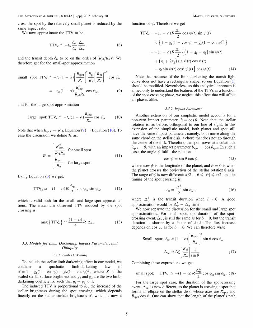
To visualize the expected TTVs derived by our analyticalapproximation for non-vanishing impact parameter cases, weplotted in Figure 4 the calculated TTVs for different values ofthe impact parameter, with the large-spot approximation, using

=R R* 0.15spot and =R R* 0.05pl values. We chose a typicalparameter for a transiting system—a planet orbiting a star withsolar radius in a three-day orbit. The duration of the transit(mid-ingress to mid-egress) is about 2.62 hr, the value onwhich we based our estimations.One can see in the figure that the amplitude of the induced

TTV is about five minutes. The derived TTVs display almostlinear slope as a function of the spot-crossing position, up to amaximum at distance of 0.6–0.85 stellar radii from the center ofthe stellar disk, and then a sharp drop to zero at the edge of thestellar disk.

4. COMPARISON WITH NUMERICAL SIMULATIONS

As noted in the introduction, Boisse et al. (2012) andOshagh et al. (2013a) developed a numerical tool, SOAP-T,7 tosimulate stellar photometric modulations induced by a rotatingspot, including a planetary transit light curve which includes aspot-crossing event. Oshagh et al. (2013b) used SOAP-T toderive detailed transit light curves, and then fitted them withtransit templates to obtain the expected TTVs, very similar towhat is performed when deriving the TTVs from theKepler actual data (e.g., Mazeh et al. 2013). This is a muchmore accurate derivation than that of the previous section,where we estimated the TTVs by the center-of-light approach.It is therefore useful to compare the TTVs obtained by ouranalytical approximation with the ones derived with the SOAP-T numerical code and the transit fitting.To do that we perform in this section two comparisons. First,

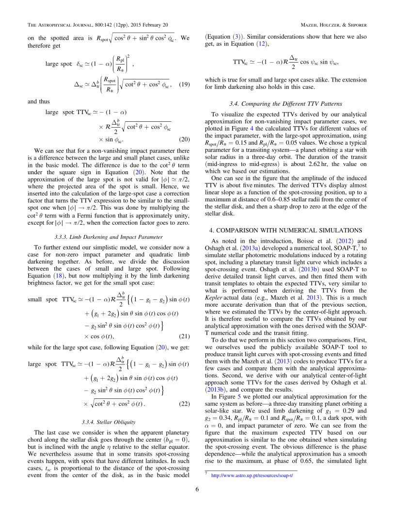
we ourselves used the publicly available SOAP-T tool toproduce transit light curves with spot-crossing events and fittedthem with the Mazeh et al. (2013) codes to produce TTVs for afew cases and compare them with the analytical approxima-tions. Second, we derive with our analytical center-of-lightapproach some TTVs for the cases derived by Oshagh et al.(2013b), and compare the results.In Figure 5 we plotted our analytical approximation for the

same system as before—a three-day transiting planet orbiting asolar-like star. We used limb darkening of g1 = 0.29 andg2 = 0.34, =R R* 0.1pl and =R R* 0.1spot , a dark spot, witha = 0, and impact parameter of zero. We can see from thefigure that the maximum expected TTV based on ourapproximation is similar to the one obtained when simulatingthe spot-crossing event. The obvious difference is the phasedependence—while the analytical approximation has a smoothrise to the maximum, at phase of 0.65, the simulated light

7 http://www.astro.up.pt/resources/soap-t/

6

The Astrophysical Journal, 800:142 (12pp), 2015 February 20 Mazeh, Holczer, & Shporer

curves yielded TTVs that are quite small for most phases, andrise sharply toward the maximum at phase 0.8.

The reason for this difference comes from the differentapproaches of obtaining the TTV. The approach that fits amodel to the simulated light curve sometimes ignores the“bump” in the light curve caused by the spot-crossing event,yielding a small TTV, while the center-of-light model is, infact, integrating over the whole transit light curve. We will seethis difference again and again. Nevertheless, this differencedoes not change the result of this paper—the negative(positive) correlation for prograde (retrograde) motion, as willbe shown below.

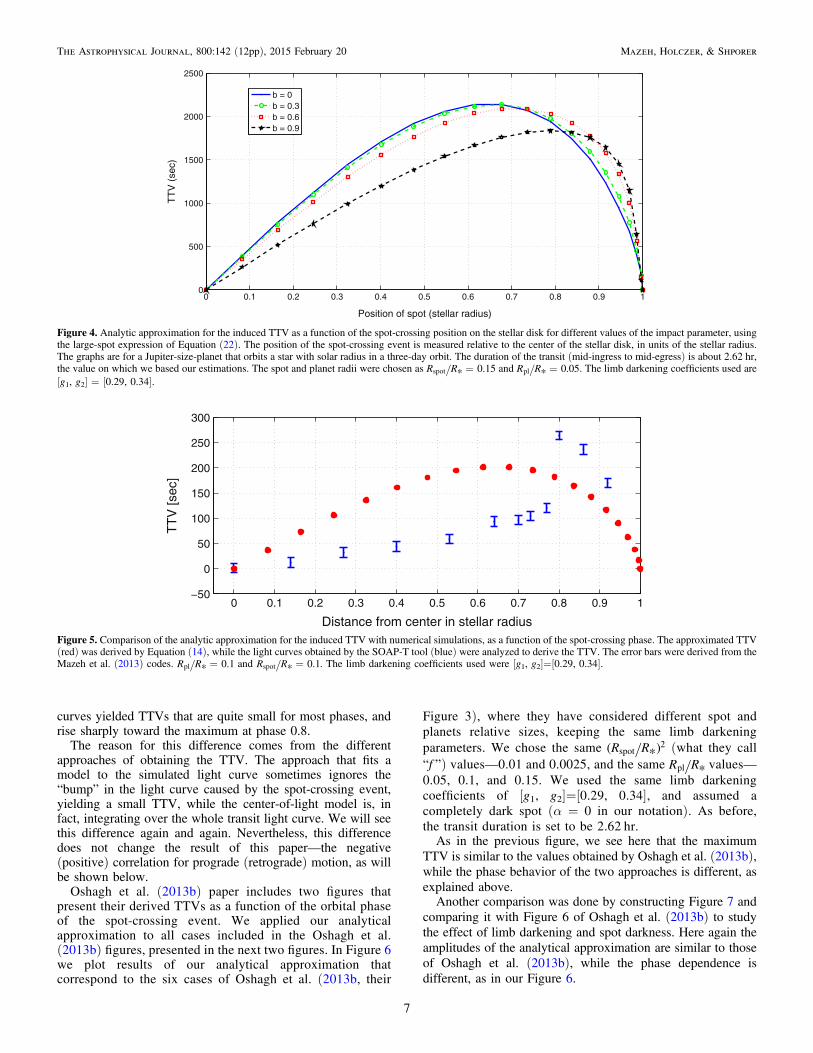
Oshagh et al. (2013b) paper includes two figures thatpresent their derived TTVs as a function of the orbital phaseof the spot-crossing event. We applied our analyticalapproximation to all cases included in the Oshagh et al.(2013b) figures, presented in the next two figures. In Figure 6we plot results of our analytical approximation thatcorrespond to the six cases of Oshagh et al. (2013b, their

Figure 3), where they have considered different spot andplanets relative sizes, keeping the same limb darkeningparameters. We chose the same R R( *)spot

2 (what they call“f ”) values—0.01 and 0.0025, and the same R R*pl values—0.05, 0.1, and 0.15. We used the same limb darkeningcoefficients of [g1, g2]=[0.29, 0.34], and assumed acompletely dark spot (α = 0 in our notation). As before,the transit duration is set to be 2.62 hr.As in the previous figure, we see here that the maximum

TTV is similar to the values obtained by Oshagh et al. (2013b),while the phase behavior of the two approaches is different, asexplained above.Another comparison was done by constructing Figure 7 and

comparing it with Figure 6 of Oshagh et al. (2013b) to studythe effect of limb darkening and spot darkness. Here again theamplitudes of the analytical approximation are similar to thoseof Oshagh et al. (2013b), while the phase dependence isdifferent, as in our Figure 6.

Figure 4. Analytic approximation for the induced TTV as a function of the spot-crossing position on the stellar disk for different values of the impact parameter, usingthe large-spot expression of Equation (22). The position of the spot-crossing event is measured relative to the center of the stellar disk, in units of the stellar radius.The graphs are for a Jupiter-size-planet that orbits a star with solar radius in a three-day orbit. The duration of the transit (mid-ingress to mid-egress) is about 2.62 hr,the value on which we based our estimations. The spot and planet radii were chosen as =R R* 0.15spot and =R R* 0.05pl . The limb darkening coefficients used are[g1, g2] = [0.29, 0.34].

Figure 5. Comparison of the analytic approximation for the induced TTV with numerical simulations, as a function of the spot-crossing phase. The approximated TTV(red) was derived by Equation (14), while the light curves obtained by the SOAP-T tool (blue) were analyzed to derive the TTV. The error bars were derived from theMazeh et al. (2013) codes. =R R* 0.1pl and =R R* 0.1spot . The limb darkening coefficients used were [g1, g2]=[0.29, 0.34].

7

The Astrophysical Journal, 800:142 (12pp), 2015 February 20 Mazeh, Holczer, & Shporer

5. ANALYTICAL APPROXIMATION FOR THE STELLARPHOTOMETRIC SLOPES

We turn now to approximate the local photometric slope atthe time of the transit, assuming as before that the stellarbrightness is modulated by a single circular spot.

For no limb darkening and null impact parameter weapproximate the stellar flux, modulated by the spot as

y y- - ⩽ ⩽F t t π π*( ) 1 cos ( ), for 2 2, (23)

where is the observed amplitude of the photometricmodulation. This is so because the spot area on the stellardisk is reduced by the aspect ratio ycos . The derivative of thestellar photometric brightness is therefore

w y F t t˙*( ) * sin ( ). (24)

The amplitude of the observed stellar photometric modula-tion is a function of the spot radius and darkness. To expressthis relation we introduce the b< <0 1 parameter, whichaccounts for the possibility that the spot crossed by the planet

might not be the only spot that contributes to the stellarmodulation with the observed phase. Therefore, β measures theratio of the area of the spot being crossed by the planet to thetotal neighboring spotted area that causes the photometricmodulation with the same phase. The total stellar modulationdue to the spots, relative to the maximum stellar brightness, is

ab- æ

èçççç

ö

ø÷÷÷÷

R

R

1

*. (25)

spot2

In the case of limb darkening, the brightness of the spottedstar takes the form

y y

y

- - -

- -

}

{F t t g t

g t

*( ) 1 cos ( ) 1 (1 cos ( ))

(1 cos ( )) , (26)

1

22

as the photometry is modulated by the aspect ratio and the limbdarkening at the spot’s location. The photometric derivative is

Figure 6. Analytic approximation for the induced TTV as a function of the spot-crossing phase for different spot and planet sizes. Expected TTVs were derived usingEquation (14). Rp/Rs is planet to star radius ratio and f is spot to star radius ratio squared. The limb darkening coefficients used are [g1, g2]=[0.29, 0.34].

Figure 7. Expected TTVs for different limb darkening parameters, using our analytical approximation for = =R R R R* * 0.1pl spot . The limb darkening coefficientswere in case 1 [g1, g2] = [0.29, 0.34], in case 2 [0.38, 0.37], in case 3 [0.6, 0.16], and in case 4 [0.29, 0.34]. In case 4 the spot has half of the stellar brightness (a = 0.5), and the spot size increased by 1.4, in order to get similar amplitude of the TTVs.

8

The Astrophysical Journal, 800:142 (12pp), 2015 February 20 Mazeh, Holczer, & Shporer

then:

w y

y y

y y

= - -

+ +

-

{

}

( )( )

F t g g t

g g t t

g t t

˙*( ) * 1 sin ( )

2 4 sin ( ) cos ( )

3 sin ( ) cos ( ) . (27)

1 2

1 2

22

The stellar photometry for the non-vanishing impactparameter is expressed as in Equation (23), but now

y q w=t tcos ( ) sin cos * , and therefore the stellar photometryderivative is

w q f F t t˙*( ) * sin sin ( ), (28)

where t is the time since the spot was in the middle of its trail,on the projection of the stellar spin (see below) on the stellardisk, and w* is the stellar rotation rate, as explained inSection 3.3.4.

For the non-vanishing impact parameter and stellar limbdarkening the stellar photometry is

q f q f

q f

- - -

- -

}

{F t t g t

g t

*( ) 1 sin cos ( ) 1 (1 sin cos ( ))

(1 sin cos ( )) (29)

1

22

and its derivative is

w q f

q f f

q f f

- -

+ +

-

{

}

( )( )

F t g g t

g g t t

g t t

˙*( ) * 1 sin sin ( )

2 4 sin sin ( ) cos ( )

3 sin sin ( ) cos ( ) . (30)

1 2

1 22

23 2

When the obliquity of the system is non-vanishing, the spotmoves on a chord orthogonal to the projection of the stellarrotational axis, at a colatitude qspot, with q=b cosspot spot. Thespot chord is different from that of the planet, which we assumegoes through the center of the stellar disk. Because of theinclination of the transit chord, at the time of crossing

q w y h=tsin sin * sin cos (31)spot sc

where t is the time since the spot was in the middle of its trail,on the projection of the stellar spin on the stellar disk, and w* isthe stellar rotation rate. Therefore, the stellar photometricderivative is like Equations (28) or (30), except for a qsin spot

factor. Note that when h π 2 then F t˙*( ) 0, because the

spot-crossing effect occurs near the photometric maximum, andtherefore the correlation with the TTVs becomes difficult todetect.

6. THE CORRELATION BETWEEN TTVsc AND THESTELLAR PHOTOMETRIC SLOPES

We are now ready to consider the expected correlationbetween the TTVs induced by the spot-crossing events and thelocal slope of the stellar photometry at the time of the transit.

6.1. TTV as a Function of the Photometric Slope

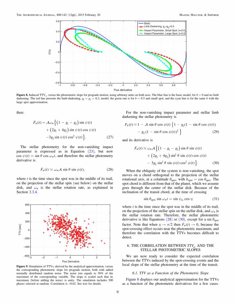
Figure 8 displays our analytical approximation for the TTVsas a function of the photometric derivatives for a few cases.

Figure 8. Induced TTVsc versus the photometric slope for prograde motion, using arbitrary units on both axes. The blue line is the basic model, for b = 0 and no limbdarkening. The red line presents the limb-darkening, = =g g 0.31 2 , model, the green one is for b = 0.5 and small spot, and the cyan line is for the same b with thelarge spot approximation.

Figure 9. Simulation of TTVs, derived by the analytical approximation, versusthe corresponding photometric slope for prograde motion, both with addednormally distributed random noise. The noise rms equals to 50% of themaximum of the corresponding variable. The slope is scaled such that itsmaximum (before adding the noise) is unity. The simulation includes 500phases selected at random. Correlation is −0.62. See text for details.

9

The Astrophysical Journal, 800:142 (12pp), 2015 February 20 Mazeh, Holczer, & Shporer

The figure shows that the slope of the stellar brightness at thetime of each transit and the corresponding induced TTV haveopposite signs for prograde motion, and therefore we expectnegative correlation between the two. Obviously, the slope andthe induced TTV have the same sign for retrograde motion,because the argument presented in Section 2 and plotted inFigures 1 and 2 still holds, and therefore a positive correlationis expected in such a case.

6.2. Correlation as a Function of Noise and Number ofObserved Transits

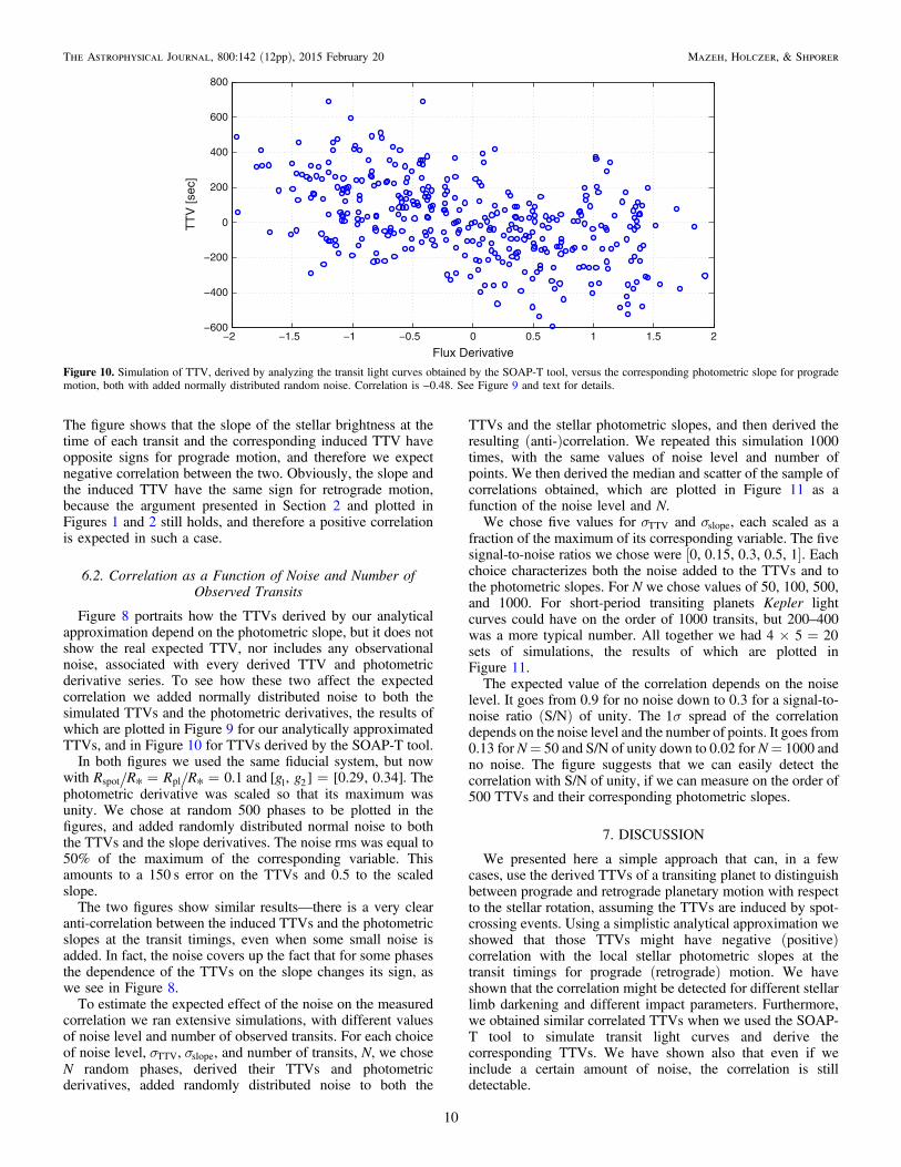
Figure 8 portraits how the TTVs derived by our analyticalapproximation depend on the photometric slope, but it does notshow the real expected TTV, nor includes any observationalnoise, associated with every derived TTV and photometricderivative series. To see how these two affect the expectedcorrelation we added normally distributed noise to both thesimulated TTVs and the photometric derivatives, the results ofwhich are plotted in Figure 9 for our analytically approximatedTTVs, and in Figure 10 for TTVs derived by the SOAP-T tool.

In both figures we used the same fiducial system, but nowwith = =R R R R* * 0.1spot pl and =g g[ , ] [0.29, 0.34]1 2 . Thephotometric derivative was scaled so that its maximum wasunity. We chose at random 500 phases to be plotted in thefigures, and added randomly distributed normal noise to boththe TTVs and the slope derivatives. The noise rms was equal to50% of the maximum of the corresponding variable. Thisamounts to a 150 s error on the TTVs and 0.5 to the scaledslope.

The two figures show similar results—there is a very clearanti-correlation between the induced TTVs and the photometricslopes at the transit timings, even when some small noise isadded. In fact, the noise covers up the fact that for some phasesthe dependence of the TTVs on the slope changes its sign, aswe see in Figure 8.

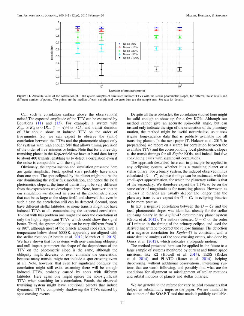
To estimate the expected effect of the noise on the measuredcorrelation we ran extensive simulations, with different valuesof noise level and number of observed transits. For each choiceof noise level, sTTV, sslope, and number of transits, N, we choseN random phases, derived their TTVs and photometricderivatives, added randomly distributed noise to both the

TTVs and the stellar photometric slopes, and then derived theresulting (anti-)correlation. We repeated this simulation 1000times, with the same values of noise level and number ofpoints. We then derived the median and scatter of the sample ofcorrelations obtained, which are plotted in Figure 11 as afunction of the noise level and N.We chose five values for sTTV and sslope, each scaled as a

fraction of the maximum of its corresponding variable. The fivesignal-to-noise ratios we chose were [0, 0.15, 0.3, 0.5, 1]. Eachchoice characterizes both the noise added to the TTVs and tothe photometric slopes. For N we chose values of 50, 100, 500,and 1000. For short-period transiting planets Kepler lightcurves could have on the order of 1000 transits, but 200–400was a more typical number. All together we had ´ =4 5 20sets of simulations, the results of which are plotted inFigure 11.The expected value of the correlation depends on the noise

level. It goes from 0.9 for no noise down to 0.3 for a signal-to-noise ratio (S/N) of unity. The s1 spread of the correlationdepends on the noise level and the number of points. It goes from0.13 for N= 50 and S/N of unity down to 0.02 for N= 1000 andno noise. The figure suggests that we can easily detect thecorrelation with S/N of unity, if we can measure on the order of500 TTVs and their corresponding photometric slopes.

7. DISCUSSION

We presented here a simple approach that can, in a fewcases, use the derived TTVs of a transiting planet to distinguishbetween prograde and retrograde planetary motion with respectto the stellar rotation, assuming the TTVs are induced by spot-crossing events. Using a simplistic analytical approximation weshowed that those TTVs might have negative (positive)correlation with the local stellar photometric slopes at thetransit timings for prograde (retrograde) motion. We haveshown that the correlation might be detected for different stellarlimb darkening and different impact parameters. Furthermore,we obtained similar correlated TTVs when we used the SOAP-T tool to simulate transit light curves and derive thecorresponding TTVs. We have shown also that even if weinclude a certain amount of noise, the correlation is stilldetectable.

Figure 10. Simulation of TTV, derived by analyzing the transit light curves obtained by the SOAP-T tool, versus the corresponding photometric slope for progrademotion, both with added normally distributed random noise. Correlation is −0.48. See Figure 9 and text for details.

10

The Astrophysical Journal, 800:142 (12pp), 2015 February 20 Mazeh, Holczer, & Shporer

Can such a correlation surface above the observationalnoise? The expected amplitude of the TTV can be estimated byEquations (11) and (13). For example, a system with

R R R0.1 *spot pl , a- (1 ) 4 0.25, and transit durationof 3 hr should show an induced TTV on the order offive minutes. So, we can expect to observe the (anti-)correlation between the TTVs and the photometric slopes onlyfor systems with high enough S/N that allows timing precisionof the order of five minutes or better. Note that for a three-daytransiting planet in the Kepler field we have at hand data for upto about 400 transits, enabling us to detect a correlation even ifthe noise is comparable with the signal.

Obviously, the approximation and simulation presented hereare quite simplistic. First, spotted stars probably have morethan one spot. The spot eclipsed by the planet might not be theone dominating the stellar flux modulation, and hence the localphotometric slope at the time of transit might be very differentfrom the expressions we developed here. Note, however, that inour simulation we allowed an error of the photometric slopethat can be as large as the slope itself, and showed that even insuch a case the correlation still can be detected. Second, spotshave different stellar latitudes, so some transits might not haveinduced TTVs at all, contaminating the expected correlation.To deal with this problem one might consider the correlation ofonly the highly significant TTVs, which could show the signalbetter. Third, the system obliquity can be very different from 0or 180 , although most of the planets around cool stars, with atemperature below about 6000 K, apparently are aligned withthe stellar rotation (Albrecht et al. 2012; Mazeh et al. 2015).We have shown that for systems with non-vanishing obliquityand null impact parameter the shape of the dependence of theTTV on the photometric slope is the same, although theobliquity might decrease or even eliminate the correlation,because many transits might not include a spot-crossing eventat all. Note, however, that even for significant obliquity thecorrelation might still exist, assuming there will be enoughinduced TTVs, probably caused by spots with differentlatitudes. Here again one might ignore the non-significantTTVs when searching for a correlation. Fourth, the observedtransiting system might have additional planets that inducedynamical TTVs, completely shadowing the TTVs caused byspot crossing events.

Despite all these obstacles, the correlation studied here mightbe solid enough to show up for a few KOIs. Although ourmethod cannot give an accurate spin–orbit angle, but caninstead only indicate the sign of the orientation of the planetarymotion, the method might be useful nevertheless, as it usesKepler long-cadence data that is publicly available for alltransiting planets. In the next paper (T. Holczer et al. 2015, inpreparation) we report on a search for correlation between theavailable TTVs and the corresponding local photometric slopesat the transit timings for all Kepler KOIs, and indeed find fiveconvincing cases with significant correlations.The approach described here can in principle be applied to

any eclipsing system, whether it is a transiting planet or astellar binary. For a binary system, the induced observed minuscalculated ( -O C) eclipse timings can be estimated with thesmall-spot approximation, for which the planetary radius is thatof the secondary. We therefore expect the TTVs to be on thesame order of magnitude as for transiting planets. However, aseclipses in binaries are usually deeper and longer than theplanetary transits, we expect the -O Cs in eclipsing binariesto be more precise.In fact, a negative correlation between the -O Cs and the

local photometric slopes was identified already for the stellareclipsing binary in the Kepler-47 circumbinary planet system(Orosz et al. 2012). The authors detected -O C on the orderof 1 minute in the timing of the primary eclipse, and used thederived linear trend to correct the eclipse timings. The detectionof a negative correlation for Kepler-47 is consistent with amore detailed analysis of the spot-crossing events, also done byOrosz et al. (2012), which indicates a prograde motion.The method presented here can be applied in the future to a

large sample of systems monitored by current and future spacemissions, like K2 (Howell et al. 2014), TESS (Rickeret al. 2014), and PLATO (Rauer et al. 2014), helpingdiscovering, without additional observations, interesting sys-tems that are worth following, and possibly find what are theconditions for alignment or misalignment of stellar rotationsand orbital motions of planets and stellar binaries.

We are grateful to the referee for very helpful comments thathelped us substantially improve the paper. We are thankful tothe authors of the SOAP-T tool that made it publicly available.

Figure 11. Absolute value of the correlation of 1000 system samples of simulated induced TTVs with the stellar photometric slopes, for different noise levels anddifferent number of points. The points are the median of each sample and the error bars are the sample rms. See text for details.

11

The Astrophysical Journal, 800:142 (12pp), 2015 February 20 Mazeh, Holczer, & Shporer

The research leading to these results has received funding fromthe European Research Council under the EU’s SeventhFramework Programme (FP7/(2007-2013)/ ERC Grant Agree-ment No. 291352). T. M. also acknowledges support from theIsrael Science Foundation (grant No. 1423/11) and the IsraeliCenters of Research Excellence (I-CORE, grant No. 1829/12).T. M. is grateful to the Jesus Serra Foundation Guest Programand to Hans Deeg and Rafaelo Rebolo, that enabled his visit tothe Instituto de Astrofsica de Canarias, where the last stage ofthis research was completed. This work was performed in partat the Jet Propulsion Laboratory, under contract with theCalifornia Institute of Technology (Caltech) funded by NASAthrough the Sagan Fellowship Program executed by the NASAExoplanet Science Institute.

REFERENCES

Albrecht, S., Reffert, S., Snellen, I., Quirrenbach, A., & Mitchell, D. S. 2007,A&A, 474, 565

Albrecht, S., Reffert, S., Snellen, I. A. G., & Winn, J. N. 2009, Natur, 461, 373Albrecht, S., Winn, J. N., Carter, J. A., Snellen, I. A. G., & de Mooij, E. J. W.

2011, ApJ, 726, 68Albrecht, S., Winn, J. N., Johnson, J. A., et al. 2012, ApJ, 757, 18Albrecht, S., Winn, J. N., Torres, G., et al. 2014, ApJ, 785, 83Barnes, J. W. 2009, ApJ, 705, 683Barnes, J. W., Linscott, E., & Shporer, A. 2011, ApJS, 197, 10Batalha, N. M., Rowe, J. F., Bryson, S. T., et al. 2013, ApJS, 204, 24Batygin, K. 2012, Natur, 491, 418Boisse, I., Bonfils, X., & Santos, N. C. 2012, A&A, 545, A109Chaplin, W. J., Sanchis-Ojeda, R., Campante, T. L., et al. 2013, ApJ, 766, 101Dawson, R. I. 2014, ApJL, 790, LL31Deming, D., Sada, P. V., Jackson, B., et al. 2011, ApJ, 740, 33Désert, J.-M., Charbonneau, D., Demory, B.-O., et al. 2011, ApJS, 197, 14Fabrycky, D. C., Ford, E. B., Steffen, J. H., et al. 2012, ApJ, 750, 114Fabrycky, D., & Tremaine, S. 2007, ApJ, 669, 1298Gizon, L., & Solanki, S. K. 2003, ApJ, 589, 1009Groot, P. J. 2012, ApJ, 745, 55Hartman, J. D., Bakos, G. Á, Noyes, R. W., et al. 2011, AJ, 141, 166

Hansen, B. M. S. 2012, ApJ, 757, 6Hébrard, G., Ehrenreich, D., Bouchy, F., et al. 2011, A&A, 527, L11Hirano, T., Sanchis-Ojeda, R., Takeda, Y., et al. 2012, ApJ, 756, 66Hirano, T., Sanchis-Ojeda, R., Takeda, Y., et al. 2014, ApJ, 783, 9Holt, J. R. 1893, A&A, 12, 464Howell, S. B., Sobeck, C., Haas, M., et al. 2014, PASP, 126, 398Irwin, J., Aigrain, S., Bouvier, J., et al. 2009, MNRAS, 392, 1456Mazeh, T., Nachmani, G., Holczer, T., et al. 2013, ApJS, 208, 16Mazeh, T., Peretz, H., McQuillan, A., et al. 2015, ApJ, in press

(arXiv:1501.01288)McLaughlin, D. B. 1924, ApJ, 60, 22McQuillan, A., Mazeh, T., & Aigrain, S. 2014, ApJS, 211, 24Moutou, C., Díaz, R. F., Udry, S., et al. 2011, A&A, 533, A113Naoz, S., Farr, W. M., Lithwick, Y., Rasio, F. A., & Teyssandier, J. 2011,

Natur, 473, 187Nutzman, P. A., Fabrycky, D. C., & Fortney, J. J. 2011, ApJL, 740, L10Orosz, J. A., Welsh, W. F., Carter, J. A., et al. 2012, Sci, 337, 1511Oshagh, M., Boisse, I., Boué, G., et al. 2013a, A&A, 549, A35Oshagh, M., Santos, N. C., Boisse, I., et al. 2013b, A&A, 556, A19Queloz, D., Eggenberger, A., Mayor, M., et al. 2000, A&A, 359, L13Rauer, H., Catala, C., Aerts, C., et al. 2014, ExA, 38, 249Ricker, G. R., Winn, J. N., Vanderspek, R., et al. 2014, Proc. SPIE,

9143, 20Rossiter, R. A. 1924, ApJ, 60, 15Sanchis-Ojeda, R., & Winn, J. N. 2011, ApJ, 743, 61Sanchis-Ojeda, R., Fabrycky, D. C., Winn, J. N., et al. 2012, Natur, 487, 449Sanchis-Ojeda, R., Winn, J. N., Holman, M. J., et al. 2011, ApJ, 733, 127Sanchis-Ojeda, R., Winn, J. N., Marcy, G. W., et al. 2013, ApJ, 775, 54Schlaufman, K. C. 2010, ApJ, 719, 602Schlesinger, F. 1910, PAllO, 1, 123Shporer, A., Brown, T., Mazeh, T., & Zucker, S. 2012, NewA, 17, 309Slawson, R. W., Prša, A., Welsh, W. F., et al. 2011, AJ, 142, 160Szabo, G. M., et al. 2011, ApJL, 736, L4Szabó, R., Szabó, G. M., Dálya, G., et al. 2013, A&A, 553, A17Triaud, A. H. M. J., Collier Cameron, A., Queloz, D., et al. 2010, A&A,

524, A25Triaud, A. H. M. J., Hebb, L., Anderson, D. R., et al. 2013, A&A, 549, A18Winn, J. N., Johnson, J. A., Marcy, G. W., et al. 2006, ApJL, 653, L69Winn, J. N., Fabrycky, D., Albrecht, S., & Johnson, J. A. 2010, ApJL,

718, L145Winn, J. N., Howard, A. W., Johnson, J. A., et al. 2011, AJ, 141, 63

12

The Astrophysical Journal, 800:142 (12pp), 2015 February 20 Mazeh, Holczer, & Shporer