Time-variant CAPM: Learning about Factor Loading

Jiho Han

April 2006

ABSTRACT 

Adrian and Franzoni (2005) suggest that beta of a stock is determined by the factor loading of its unobservable long-run beta. The fundamental idea behind this model is that investors engage in a learning process of estimating this long-run beta. In this paper, a variation of this model is tested. Instead of estimating long-run beta, investors try to learn about factor loading. Given the long-run beta and the upcoming level of risk, investors must form the optimal factor loading that minimizes the pricing error. The evolution of the factor loading assumes to follow an AR(1) process. The mispricing results are as equally successful as Adrian’s model. The momentum in the optimal factor loading is confirmed. During the transitional business-cycle periods, the factor loading seems to be more volatile.

1. Introduction

Sharpe (1964) and Linter (1965) introduce the Capital Asset Pricing Model (CAPM), which provide

a first comprehensive mechanism of rational investors’ behaviors. Despite its theoretical elegance and

simplicity, CAPM makes many assumptions that are quite unrealistic in the derivation of the model. For

example, CAPM assumes an ideal, market-efficient situation where all the investors share same

information and same utility function. From structural point of view, the most serious problem of CAPM

is to use OLS procedure to estimate betas. Each observation of historical return of a specific

stock/portfolio is a time-series data, which inevitably involves non-zero autocorrelation. However, in spite

of all these problems, the reason that CAPM is scorned by many investors is that CAPM have failed to

cope with the empirical observations, especially for the periods after 1960s. Fama and French (1992) find

pervasive evidence that CAPM is unable to explain return on size and book-to-market (BE/ME) sorted

portfolios.

Naturally, many researchers and scholars begin to look for alternative theories. Two mainstream

branches of researchers arise in order to improve CAPM: (1) Multi-factor models and (2) Conditional

CAPM. The former group renounces a univariate structure and extends to a multi-dimensional model.

Fama and French (1996) suggest an influential three-factor model, which includes market risk factor (β),

size factor (SMB), value factor (HML) to account for the problem they address previously. While this

model shows highly improved predictive power, it lacks an underlying explanation of why market

behaves in this particular way (Campbell 2004).

Another branch of researches preserves a one-factor model and proposes that CAPM holds only

conditionally. In other words, although the cross-sectional CAPM holds true at any given time t, the

unconditional CAPM may fail unconditionally. Jagannathan and Wang (1996) model the evolution of the

conditional distribution returns at time t as a function of lagged state variables. From this structure, they

derive that the covariance between the market and portfolio returns, i.e., betas, as affine functions of these

variables. Lettau and Ludvigson (2001) find that the betas of value stocks are highly correlated with

consumption growth rate. Hence, they suggest the use of a conditional variable CAY1 as a controlling

variable when estimating betas. Upon these research results, Adrian and Franzoni (2005) take learning

into consideration. They argue that the unobservability of true betas causes investors to engage in learning

process. In their Learning-CAPM, a beta evolves by finding a weighted average of the previous period

long-run and current betas. Investors continuously “update” their long-run and current betas since these

values are not observable. It is important to note that factor loading, or weight, remains fixed in Learning-

CAPM.

Inspired by Adrian and Franzoni, this paper provides a variation of Learning-CAPM under totally

different assumptions. Instead of assuming the unobservability of betas, investors as a whole are assumed

to have the estimates for long-run and forecasted upcoming period risk. From these two established risk

measures, investors must form the optimal weight, or the factor loading Ft, that minimizes the pricing

error. The evolution of factor loading is designed to have a momentum in a sense that it follows an AR(1)

process. While the assumption of having upcoming period risk seems rather bold, many researches show

that investors have some ability to forecast near-future risk/return. Moreover, this assumption does not

imply that individual investors have same upcoming level of risk; it is an aggregated market estimate of

risk for the next period. The point of this paper is to examine a market’s response when forecasted

upcoming risk is available. In that sense, the evolution of factor loading describes how an efficient market

works because it represents stock’s sensitivity to current market news.

The learning factor loading model is differentiated from the presented literature in two ways. First, it

endorses an active investment situation. Unlike Learning-CAPM where investors merely updates their

1 Lettau and Ludvigson (2001). CAY is an acronym for log consumption, C, log asset, A, and log labor income, Y.

risk estimates, the factor loading model hypothesizes that investors develop new index of risk each time

period by properly mixing up their long-run and forecasted risk. Secondly, in extension of the first point,

the learning factor loading model admits investors’ forecasting ability and its momentum effect on returns.

This is a departure from Jagannathan and Wang (1996) in a sense that forecasted risk is used to model

betas instead of lagged state variables.

From structural point, the learning factor loading model also has two limitations that pertain to the

points made in the previous paragraph. First, the learning factor model does not provide answers on how a

market evaluates long-run and upcoming level of risk. In this paper, the OLS betas estimated from past

60-months returns are assumed to describe the investors’ estimates of long-run risk whereas the forecasted

risks are calculated under Bayesian setting given the next-period returns. In future research, these values

can be replaced by macro factors or some investors’ consensus data such as, IBES forecasts. Secondly, the

importance of factor loading depends on the relationship between long-run and upcoming betas. Suppose

the situation where the long-run and forecasted betas move in the exactly same way. Then, the factor

loading clearly has no impact on deciding the true level of risk. Likewise, if the differences between two

risk factors are small (in absolute sense), its weighted averages would not change much by factor loadings.

In fact, this turns out be the case for large growth portfolio tested as shown in Figure 4.

For these reasons, the focus of this paper will be on the movement or variability of factor loadings, Ft,

than the actual realizations of it. For example, the variances in the factor loadings of small and value

portfolios are expected to be greater than the changes in large and growth portfolios. For these high

volatile portfolios, the discrepancies between the long-term and short-term risk factors are expected to be

high, so that factor loading plays a crucial role in determining the true risk. By the same reasoning, the

factor loading of large growth portfolios will have little impact on the true risk because these portfolios

have relatively stable returns and thus will have smoother long-run and upcoming levels of risk.

The rest of the paper is organized as follows. In Section 2, the economical and statistical literature

relevant to the topic is covered. The basic idea of Kalman filter and its application helps to understand the

quantitative aspect of the mechanism. The discussion about Adrian’s Learning-CAPM also follows. In

Section 3, the specification and the derivation of a newly proposed model will be presented. Section 4

reports the empirical result as well as the interpretation of the factor loading. Section 5 draws conclusion

for this work.

2. Related Literature

The idea of unobservable components is not new. Historically, numerous attempts have been made to

measure these unobservable components. However, it is relatively a recent event that Kalman (1960)

finds a way to estimate time-evolving unobservable components over discrete-space. In terms of

methodology, what Kalman filter does is simply alternating between predicting (prior) and updating

(posterior) the unobservable variables. Although the model is originally developed for primary use in

aerospace-related research2, it turns out that Kalman filter is widely applicable in other areas such as

economics, medicine (Jones 1984), and seismology (Shumway 1985).

From economics perspective, the alternating procedure between prediction and updating can be

viewed as learning process. For example, Martin (1990) attempts to construct a leading index for the

United States by deriving a set of weights based on Kalman filters. He models a leading index as an

AR(p*) process and finds the optimal coefficients so that the prediction error is minimized. Underlying

assumption in his work is that people learn from their prediction error and use the updated measures to

predict the future values. Likewise, Sargent, William, and Zha (2005) argue that the fluctuation of

inflation rate in the post-war period can be explained by the policymakers’ learning process. The

policymakers have a certain prior about how inflation and unemployment are related, but the true

relationship should be inferred as the results from policymaking become available.

Adrian and Franzoni (2005) incorporate this learning concept in the estimation of beta. According to

them, the tradition OLS approach ignores investors’ gain from the previous errors and, as a result, CAPM

is rejected too often. Their model focuses on the factor loading of a long-run beta, which is unobservable.

Under this framework, the object of learning is this long-run beta, which investors must form expectation

over time. In relation to this setting, the focus of this article is to model the evolution of the factor loading

2 In fact, Kalman filter plays a crucial role in development of Global Position System (GPS).

itself given the long-run beta. In fact, the idea of long-run beta tracks back to Jostova and Philipov (2005).

They introduce the idea of a “mean-reverting beta” and show that it can help to explain the size and B/M

premium of CAPM model. However, they do not take learning into consideration. On the other hand,

Adrian and Franzoni (2005) confirm this preceding statement in their Learning-CAPM.

Interestingly, another attempt to incorporate learning into practice is made from behavioral and

psychological point of view. Lakonishok, Shleifer, and Vishny (1994) claim that investors are too

optimistic about past high earning growth. Consequently, these companies tend to be small and

overvalued and, subsequently, experience serious underperformance only when the growth rate

disappoints investors. The supporting evidence for this explanation for the value premium is provided by

La Porta (1996) and La Porta el at. (1997), who show that the underperformance of stocks with low

BE/ME ratios is concentrated on earning announcement dates (Campbell 2003). Brav, Lehavy, and

Michaely (2002) also confirms this view by pointing out that analysts have high subjective expected

returns on growth stocks, consistent with the hypothesis that the value premium is due to expectation

error (Campbell 2003). Under these models, learning is not a continuous process, but rather an event that

occurs when investors realize the discrepancy between the expectation and the reality.

The following sections explain the two key concepts needed for understanding the model developed

in this paper. The first part gives a brief overview of Kalman filter and its statistical implications as well

as some warnings embedded in the filtering process. The second part is about Learning-CAPM (Adrian

and Franzoni 2005). Since it plays a central role in understanding and development of the original work in

this paper, it is worthwhile to go over their model and the result in detail.

2.1 State‐space Model and Kalman Filter 

Dynamic linear model (DML) or state-space model (SSM) was originally invented to describe the

movement of unobservable state variables, which evolve over time. The compelling fact is that these

variables only reveal themselves through the realizations of some other observable variables. Naturally,

this system of equations consists of two parts: (1) State equation that describes the transition of state

variables from time t to t+1, and (2) Observation equation that shows how state variables relate to

observable variables at time t.

Mathematically, the model can be written as follows. Let xt be a p×1 vector of state variables. Then,

1 where ~ ( 0, Q )t t t tx x w w N−= Φ ⋅ + (2.1)

is the state equation where Φ denotes the transition matrix. The observational equation is

where ~ ( 0, R )t t t t ty H x v v N= + (2.2)

with the observation matrix Ht. The error terms, wt and vt, are assumed to follow a normal distribution

with mean zero and the covariance matrix Q and R, respectively. Note that there is a time subscript for the

observation matrix Ht , but not for the transition matrix Φt.

By including the previous state variables in the current one, these equations can easily be expanded

to multi-stage setting. Note that this form embraces popular vector-autoregressive (VAR) model. It is a

trivial case where the observation matrix is an identity and the variance of the observation equation R is

zero. Relaxing the constant variance of the error terms, Equation (2.1) and (2.2) encloses ARCH model.

Moreover, while hidden Markov model and state-space shares the common characteristic of hidden

transition of state variables, state-space model do not have to satisfy Markov property.

More general form of state-space equations can include a vector of exogenous variables. These

variables serve as a controlling factor. Adrian and Franzoni (2005) tests the benefits of including several

controlling variables, such as CAY, term structure spread, and Fama French factors, in their model and

conclude that no variables other than CAY improves the result significantly. In this paper, however, these

exogenous variables are omitted because it is believed that conditional CAPM holds without the aid of

any other variables.

Kalman filter is a technique to find the solution of a state-space model parameters, such as Φ, given

the realization of y1, y2, …, yn. The solution can be found through a recursive procedure (hence, the name

filtering) that alternates between predicting and updating the unobservable measures. The filtering process

begins with some initial settings at t = 0. Under these initial values, the prediction for the next step at t = 1

is made to obtain priori state estimates. As new information becomes available, these estimates should be

updated and the resulting measures are called posteriori estimates. These updated posteriori values are

then used to obtain the next step priori estimates, and the procedure goes on. The mathematical

description of Kalman filtering process is provided in Appendix. The detailed explanation for the

procedure can be found in Welch and Bishop (2004).

It is often the case, as in this paper, that the purpose of the filtering process is to figure out the

maximum likelihood estimates of Φ, Q, and R. The estimates of x1, x2, …, xn, then, can be computed from

these parameters. As a matter of fact, finding the maximum likelihood estimates involves quite amount of

computation. Shumway and Stoffer (2000) describe the general procedures as follows:

1) Choose an initial values for the parameters, say Θ(0) = { Φ(0), Q(0), R(0) }.

2) Run the Kalman filter, using this initial parameter values. Obtain a set of innovations and corresponding covariances, say, { εt

(0); t = 1,…, n } and { Σt ; t = 1,…, n }. 3) Using these innovations, apply Newton-Rhapson algorithm to find the likelihood

maximizing estimates of Θ(1).

4) Repeat the above steps until the estimates or the likelihood stabilize.

Unfortunately, the convergence of the maximum likelihood estimates to the actual values is not

guaranteed in general. The likelihood function, LY(Θ), can be written as

1

1 12 ln ( ) log | ( ) | ( ) ' ( ) ( )

n n

Y t t t tt t

L ε ε−

= =

− Θ = Σ Θ + Θ Σ Θ Θ∑ ∑

Of course, this function is a highly nonlinear function of Θ and thus the optimizing surface can be quite

rough. This implies that the likelihood maximization estimates only lead to the local maximization point

(Kahl 1983). Another problem involves initializing values. When the initial values and covariances are

not known precisely, a new error that is not included in the system is introduced. A typical solution to this

problem is to let the initial covariance matrix Σ0 large so that it compensates for the unknown initial status.

De Jong (1994) develops an extended form of Kalman filter, which can be used under diffuse situation.

Diffuse situation occurs when the initial values are unknown but can be modeled as random vectors with

arbitrarily large covariance. Theoretically, diffuse Kalman filter can handle all the issues arisen in this

problem. In this paper, however, the initial estimates are assumed to be in the correct range so that the

maximum likelihood estimates converge to the true values. Likewise, the initial covariance matrix is

assumed to be large enough to compensate for the estimates error at the initial point t = 0.

From conceptual point of view, Kalman filter can be viewed as a simple Bayesian updating scheme

that that maximizes the likelihood of the unknown parameters. It is differentiated from classical time-

series model in two ways. First, the system is divided into two separate equations, state and observation.

Secondly, the unobservable components are updated as new information comes in. It is this feature that

makes Kalman filter useful in estimating beta; when investors observe discrepancy between the expected

level of risk and the actual risk, they adjust their belief accordingly.

2.2 Learning‐CAPM 

Learning-CAPM (Adrian and Franzoni 2005) is a variation of the conditional CAPM that is based on

the belief that investors must form expectations about the true level of risk over time. Against the

criticism of Lewellen and Nagel (2005) that the success of the conditional CAPM depends on its cross-

sectional design, these authors propose a time-varying beta model under the specification of the

conditional CAPM.

With the assumption of no-arbitrage and unknown parameters of the return process, Adrian and

Franzoni (2005) provide the framework on which the conditional CAPM holds. Formally, it is written as

1 1|[ ] [ ]Mt t t t t tE R E Rβ+ += ⋅ (2.3)

where 1| 1 1 1 1ˆ [ | ] [ | ]i

t t t t t t t tE M E Rβ β β+ + + + += = . The preceding identity implicitly asserts that the market

return RM is a sufficient statistic for the pricing kernel M. These authors model the current level of beta as

an autoregressive process:

1 (1 )i i i i i it t tF B F uβ β+ = − + + (2.4)

where Bi represents the long run beta, which assumes to be unobservable. They argue that investors

engage in a learning process of continuously estimating Bi. The factor loading, Fi, is a pre-determined,

firm-specific constant that reflects how much of the historical betas should be trusted. It is important to

notice that both Bi and Fi do not have time subscript, and thus, have time-invariant nature. However, the

long-run beta Bi is the object of learning and thus its estimate is updated constantly as new information

comes in. On the other hand, the factor loading Fi is a truly time-invariant and must be estimated using

the maximum likelihood method.

The parameters of interest are the factor loading of stock i, Fi, the idiosyncratic variance of beta Q,

and the idiosyncratic variance of the return R as well as the coefficients for any exogenous variables if

there is any. With the initial estimates of Bi = βi = 1 and a diffuse3 (uninformative) prior, the model is

regressed over the period from 1926 to 2004 although the pricing error estimation focuses on the returns

after 1960s. The two authors emphasize on the reason that they focus on the latter half (after 1960s) of the

sample. In the early years up to 1960s, small and value stocks have large realizations of betas. Therefore,

it is important to start the filter at the beginning of the sample and allow enough time to form expectation

for long-run betas.

Using Learning-CAPM, the RMSE of pricing error is dropped by 24% on average of the entire

twenty-five portfolios4. The reductions in the composite pricing error5 (CPE) are higher than the RMSE

decreases. Moreover, these authors are able to provide explanation for the small and value premium.

Small and value stocks form higher long-run betas from the returns prior to 1960s. Consequently, the

current level of betas for small and value stocks are higher than the OLS estimates. The same reasoning

applies to the growth, large stocks; the slow, steady realizations of these stocks’ returns contribute to low

long-run betas. On the other hand, it is interesting to see that the factor loading Fi for small and value

stocks is higher than that of large, growth stocks. This fact implies that the long-run betas of small, value

stocks should be less trusted. Finally, Adrian and Franzoni confirm the robustness of their estimates under

different specifications of the models. In other words, the inclusion of other controlling factors, e.g., CAY,

does not affect the maximum likelihood estimates of the factor loading, Fi, and the idiosyncratic variance

of state and observational equation, R and Q.

3 It is unclear what the actual prior is. In replicating Adrian’s work, an identity matrix is used in place of the diffuse prior. In addition, note that these authors also overcome the initialization problem with uninformative prior. 4 RMSE of the original CAPM is 1.076. Learning version of CAPM yields the RMSE of 0.814. Conditioned on CAY, the RMSE from Learning-CAPM is 0.668. 5 Campbell and Vuolteenaho 2004.

3. Model Specification and Estimation Method 

The idea of long-run beta is certainly attractive and has been the subject of research for some time.

Jostova and Philipov (2005) propose to estimate a mean-reverting beta under Bayesian framework. They

suggest that the mean-reversion in betas helps to solve the size and BE/ME anomalies in CAPM. This

concept is “at the core” of Learning-CAPM as long-run beta, Bi, plays a role of mean-reverting beta. In

fact, Adrian and Franzoni succeed to some degree to explain these anomalies. The difference is that

Jostova and Philipov (2005) assume mean-reverting beta follow AR with observable parameters while

Adrian and Franzoni (2005) treat long-run beta, Bi, as a latent variable whose parameters must be

estimated.

Inspired by Adrian and Franzoni’s work (2005), this paper starts from the question: Are betas really

unobservable? While the assumptions of a long-run beta and the autoregressive evolution of betas seem

plausible, the whole problem can be viewed from a different perspective. Instead of focusing on the

evolution of long-run beta, in this paper, the spotlight is on the factor loading. It is assumed that investors

already have the estimates for security i’s long-run level of risk, Bi, as well as the forecasted upcoming

risk, βi. In the process of creating a proxy variable for upcoming beta, βi, it is assumed that a market as a

whole has an ability to predict near-future returns (Appendix). What they do not know is how to balance

the discrepancy between these two measures of risk. Hence, the factor loading, Fi, that establishes the

market equilibrium becomes the subject of interest.

In the learning factor loading (LFL) model, the investors’ evaluation of true level of risk is based on

the following equation6:

1 1| 1| 1|[ ] (1 )i i i i i it t t t t t t t t tE F B Fβ β β+ + + += = − + (3.1)

6 Unless noted specifically, the superscript i will be dropped for the remainder of this paper.

where βt = Et[βt+1|Rt+1, RMt+1] denotes the investors’ one-step ahead prediction for beta based on the next

period returns. This figure, however, is a measure of risk only for the upcoming period and does not have

any long-term implication. The assumption of upcoming beta implicitly states that investors are interested

in knowing the true level of risk that affects the long-term returns.

While taking the similar structure as to Adrian and Franzoni’s model, the time subscripts on Bt and βt

indicate that these measures are now time-variant. These risk parameters are assumed to be observable

and known to all investors, and for that reason, the expectations on the right side terms are unnecessary. It

is crucial to point out that the evolving entity is the factor loading Ft, and not the betas. It is assumed that

the factor loading Ft follows an AR process, which serves as the state equation:

1 1t t tF F uφ ϖ+ += + + (3.2)

where ϖ is a mean-adjusting constant. Since Adrian and Franzoni’s proof on the conditional CAPM does

not depend on the evolution of beta, Equation (2.3) assumes to hold. Then, substituting Equation (3.1)

into Equation (2.3) and solving in terms of Ft, the following equation is obtained:

1 1| 1

1| 1| 1

1| 1

1 1| 1

[ ] [ ]

{(1 ) } [ ]

{( ) } [ ]

( ) [ ] [ ]

Mt t t t t t

Mt t t t t t t t

Mt t t t t t t

M Mt t t t t t t t t

E R E R

F B F E R

B F B E R

B E R F B E R

β

β

β

β

+ + +

+ + +

+ +

+ + +

= ⋅

= − +

= − +

= − ⋅ +

(3.3)

Moving the right-most term to the other side gives the observation equation for LFL model:

1 1 1 1|[ ] [ ] ( ) [ ]M Mt t t t t t t t t t tE R B E R B E R Fβ+ + + +− ⋅ = − ⋅ (3.4)

Notice that the left side of the equation is the residual from CAPM estimate based on the long-run beta.

On the other hand, the right side represents the difference in the expected returns from the long-run and

the current betas. In other words, the factor loading, Ft, onto the investors’ estimated risk, itβ , evolves by

evaluating the performance of the long-run betas. If the residual from the long-run CAPM estimates is

large, the factor loading on itβ will increase for the next period; that is, the long-run beta becomes less

trustworthy. In the opposite case, more weight will be given to the long-run beta, Bt, and, therefore, the

factor loading decreases in the next step.

Perhaps the biggest challenge that LFL-CAPM faces is to justify the question: Can investors really

estimate the upcoming level of risk? Many research results indicate that investors do have certain ability

to forecast the near-future returns. For example, Jegadeesh (1990) gives evidence of predictable behavior

of security returns over short period of time. His research finds that the negative first-order serial

correlation in monthly stock returns is highly significant. He also suggests that positive serial correlations

at longer lags may exist. The experiment done by The Wall Street Journal is another example. It compares

the performance of the randomly selected stocks to the returns of the analysts picked stocks over each

five-and one-half month period. The experiment lasts from July 1990 to September 2002; the result is that

the analysts’ choices outperform the random stocks 90 times out of 147 total contests (Ross et al. 2006).

Das, Levine, and Sivaramakrishnan (1998) witness the analysts’ ability to predict the returns although

they claim that these predictions are corrupted by the analysts’ optimism or pessimism. In LFL model,

these behavioral patterns are reflected in the evolution of the factor loading. From these results, the

assumption of investors’ access to upcoming level of risk does not seem implausible.

By itself, itβ is not a complete indicator of true level of risk; therefore, investors attempt to adjust

their estimate of true risk by correctly balancing the long-run risk and the upcoming estimates of the beta.

The degree of which such information should be reflected is the factor loading, Ft. Note that this factor

loading does not have to lie in the unit interval [0, 1]. When the differences between the long-run and

upcoming betas are small or they co-vary with each other, the factor loadings play little role; the

estimated true risk will be more or less the same. The factor loading becomes important when the

difference between the betas is big or they move in the different direction. In this case, the true risk is

affected substantially by the level of factor loading at that moment.

In this paper, the OLS betas estimated from the past 60-months returns are used in place of the long-

run betas (Figure 1). It is believed that 60-months are a period long enough for investors to form a long-

run level of risk. The reason that the OLS betas is calculated using the fixed number of returns is to allow

the time variation of the long-run risks. While Learning-CAPM requires enough initialization period for

the long-run beta takes into effect, the learning factor loading model does not require such period. On the

other hand, the upcoming level of beta, 1 1 1[ | , ]i Mt t t t tE R Rβ β + + += , is estimated using Bayesian model.

Assuming that investors correctly identify the next-period returns, their estimate of the upcoming risk is

calculated as if CAPM holds. The distribution of the long-run OLS betas is used as prior. The details can

be found in Appendix.

Given these long-run and upcoming level of risk, investors decide the optimal factor loading Ft (and

subsequently, Ft+1|t) according to Bayes rule. Since the evolution of Ft is a conditional distribution,

Kalman filter is the natural estimating scheme. To summarize, LFL-CAPM models the evolution of the

factor loading by applying Kalman filter to the following state space:

1 1

1 1 1 1| 1

OLS betas

( )

:

: estimated by Bayesian model

t t t

M Mt t t t t t t t t

t

t

F F u

R B R B R F v

B

φ ϖ

β

β

+ +

+ + + + +

= + +

− = − ⋅ + (3.6)

The normal distributions of the idiosyncratic error terms, vt and wt, are assumed. It is assumed that these

errors are uncorrelated to each other and over different time period. The autoregressive parameters, φ and

ϖ, and the standard errors of the error terms, σu and σv,, are estimated using maximum likelihood. For the

initial condition, φ0 is assumed to be 0 with the initial variance of 0.57. The initializing values for σu and

σv, are the standard deviations of the OLS betas and the market returns, respectively.

This specification of LFL model is totally different from any other models in the recent literature.

Jagannathan and Wang (1996), Harvey (1989), and Lettau and Ludvigson (2001) all see betas as

deterministic, affine functions of state variables where no ambiguity is introduced in the evolution of

betas (Adrian and Franzoni 2005). Ang and Chen (2004) and Jostova and Philipov (2004) postulate AR

process for betas, but assume that the parameters for the process is observable. Learning-CAPM by

Adrian and Franzoni (2005) is most closely related to LFL-CAPM; however, it is only interested in the

evolution of beta and pays little attention to the changes in factor loading. In contrast to all these models,

the learning factor loading model conjectures that investors attempt to reconcile the discrepancy between

the long-run and forecasted level of risk by learning about the past evolution of the factor loadings.

7 Assuming that the true F0 lies in the unit interval [0,1], the maximum variance possible is 0.5 The maximum variance is used to prevent the initialization problem mentioned in Section 2.1.

4. Empirical Result and Discussion 

In this section, the learning factor loading model is put into practice and tested over a set of empirical

data. The six portfolios constructed by Fama and French (1993) are used for regression because the

traditional CAPM troubles the most to explain the size and value abnormal returns from these portfolios.

As claimed by Adrian and Franzoni (2005), these anomalies are the types of mispricing that is “most

likely to be related to learning problem.” However, the underlying mechanisms are different. Adrian and

Franzoni explain that the high level of long-run betas from the past affects the current betas, which makes

them higher than the OLS estimates (Figure 2). LFL model suggests that investors’ forecasting ability and

continuing underperformance of the OLS betas together explain the value/size premiums.

The six portfolios are formed by double sorting the stocks of NYSE, AMEX, and NASDAQ by the

size and the book-to-market (BE/ME) ratios. These portfolios are constructed at the end of June each year

and the value-weighted returned are reported. The size breakpoint is the NYSE market equity median at

the end of June of year t. The book-to-market ratios breakpoints are 30th and 70th percentile of all the

stocks. Given these portfolios are used widely in the literature, further explanation is omitted. The

following table summarizes the breakdown of the portfolios.

In order to compare the results with Learning-CAPM, the regression is performed over the time

periods from 1926 to 2005. With respect to Adrian’s argument, Learning-CAPM is given with the

adequate amount of time to develop the evolution of long-run beta. Moreover, it is important to point out

that the factor loading, Fi, of Learning-CAPM and the time-evolving factor loading, Ft, in LFL model

should not be confused. In Learning-CAPM, the factor loading is the weight given to the current beta; in

LFL model, the factor loading is the weight to the upcoming betas. In other words, these values are the

weights for the two different and unrelated measures of risk.

The maximum likelihood estimates are calculated by the procedures described in Section 2.1. Table

1 summarizes the estimated parameters for each model. The first panel regards Learning-CAPM. The

estimated values are substantially different from Adrian’s report because: (1) the portfolios are formed by

different method. (2) These authors change the returns to quarterly figures, so that they can condition on

exogenous variables. In this paper, only the unconditioned version of Learning-CAPM is replicated.

Although the estimated values are considerably different, looking at the calculated betas, the downward

trends in the long-run betas of small value portfolio is still evident (Figure 2). It turns out that the average

of both Learning-CAPM and LFL-model betas (over the period from 1960 to 2005) are not big enough to

justify the value premium although they are bigger than the OLS measure (Table 1). However, there is a

24% reduction in RMSE in both learning-augmented models.

As mentioned previously, this paper focuses on the pricing errors for the period after 1960s. However,

the use of Kalman filter raises an issue of how to calculate the mispricing. In order to solve this problem,

the same method adopted by Adrian and Franzoni is used. First, the pricing error for each month, say, αt+1,

based on one-step ahead beta is calculated. That is,

1 1 1| 1i i Mt t t t tR Rα β+ + + += − (4.1)

where βt+1|t is from Equation (3.1). Then, the average of αit+1 over the period from 1960 to 2005, denoted

by iα , is used as the mispricing (alphas) for that portfolio. Likewise, the standard error of the mispricing

estimates is calculated as follows:

2

1

( ) 1( ) where ( ) ( )1

i ni i i i

jj

SDSE SDn nαα α α α

=

= = −−∑ (4.2)

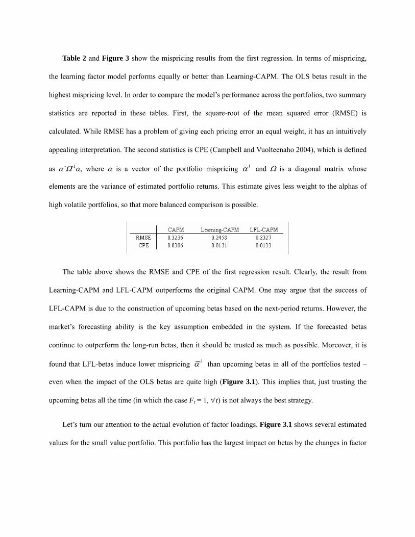
Table 2 and Figure 3 show the mispricing results from the first regression. In terms of mispricing,

the learning factor model performs equally or better than Learning-CAPM. The OLS betas result in the

highest mispricing level. In order to compare the model’s performance across the portfolios, two summary

statistics are reported in these tables. First, the square-root of the mean squared error (RMSE) is

calculated. While RMSE has a problem of giving each pricing error an equal weight, it has an intuitively

appealing interpretation. The second statistics is CPE (Campbell and Vuolteenaho 2004), which is defined

as α`Ω-1α, where α is a vector of the portfolio mispricing iα and Ω is a diagonal matrix whose

elements are the variance of estimated portfolio returns. This estimate gives less weight to the alphas of

high volatile portfolios, so that more balanced comparison is possible.

The table above shows the RMSE and CPE of the first regression result. Clearly, the result from

Learning-CAPM and LFL-CAPM outperforms the original CAPM. One may argue that the success of

LFL-CAPM is due to the construction of upcoming betas based on the next-period returns. However, the

market’s forecasting ability is the key assumption embedded in the system. If the forecasted betas

continue to outperform the long-run betas, then it should be trusted as much as possible. Moreover, it is

found that LFL-betas induce lower mispricing iα than upcoming betas in all of the portfolios tested –

even when the impact of the OLS betas are quite high (Figure 3.1). This implies that, just trusting the

upcoming betas all the time (in which the case Ft = 1, ∀t) is not always the best strategy.

Let’s turn our attention to the actual evolution of factor loadings. Figure 3.1 shows several estimated

values for the small value portfolio. This portfolio has the largest impact on betas by the changes in factor

loading8. In other words, investors have the most trouble in balancing the long-run and upcoming betas.

For this portfolio, the difference between these two betas are relatively large (compared to the others) so

that the optimal factor loading plays a crucial role. Also notice the increasing or decreasing patterns in the

factor loading. It indicates that the optimal factor loading has a momentum. For instance, suppose that

increasing the factor loading, Ft, is proven to be helpful at time t. Then, there is a high chance that

increasing the factor loading for the next period t+1 helps to reduce the pricing error. This momentum

phenomenon exists in almost all the portfolios (Figure 4). If there is no momentum in the optimal factor

loading, Kalman filter should result in an AR coefficient φ close to zero or the large variance of the state

equation, σ2u. Neither of them is the case as shown in Table 1. This is a critical evidence for LFL model

because the market’s forecasted risk – even conditioned on the next-period returns – cannot capture the

market behaviors completely.

Figure 3.1: OLS betas, Upcoming betas, LFL‐betas, and Factor Loadings. The black line is the OLS betas used as the long-run risk; the blue line represents the upcoming betas; the red line is the LFL-betas obtained by averaging the two previous betas with the factor loadings values, which are shown in dots.

0 200 400 600 800

0.0

0.5

1.0

1.5

2.0

2.5

3.0

3.5

Index

F

Small Value

8 The portfolio of the largest variability is the small growth portfolio followed by the large neutral portfolio. However, for these portfolios, the differences between the long-run and upcoming betas are too small, so that higher factor loading do not affect the resulting LFL-beta that much (Figure 4). This is the problem mentioned in the introduction.

It is unclear what causes this momentum in factor loading. Although the magnitude and frequency of

momentum in the factor loading reduce in large/growth portfolios, the patterns are still clear in all of the

portfolios (except the large/growth portfolio whose factors loadings are almost constant). With this result,

it can be hypothesized that investors’ own expectation and overconfidence on the forecasted risk/returns

can account for some of the changes in returns.

Then, what induces the changes in the optimal factor loading? It is believed that the factor loadings

are related to some macroeconomic variables. Therefore, the relationship between the factor loadings and

the business cycle is investigated. The NBER index for contraction and expansion is used to plot Figure

3.2 and Figure 3.3. Define the transitional periods as shown in the following diagram.

Figure 3.2: Factor Loading of Small Value Portfolio and the Business Cycle 

0 200 400 600 800

0.0

0.5

1.0

1.5

2.0

2.5

3.0

3.5

Index

F

Factor Loading and the Transition Periods

25%

25% 25% Trough Trough

Figure 3.3: Differences in Factor Loading at Lag 1.

0 200 400 600 800

-10

12

Index

diff(

F)

Difference in Factor Loading at Lag 1

Figure 3.2 represents the actual factor loadings while Figure 3.3 is the differences in factor loadings at

lag 1, i.e., Ft+1 – Ft . As the graphs shows clearly, the variability in factor loadings are high during the

transition period. There is no difference in directional changes between the peak- and trough-transition

periods. In other words, investors do not favor either long-run or upcoming betas just because the

economy is booming or recessing. As in the case of momentum, the high volatility during the transition

period is apparent in all of the portfolios (Figure 5). However, few exceptions are observed when the

contracting or expansionary (non-transition) periods last long, for example, over 5 years (red-boxed

period in Figure 5). Overall, the movement of the optimal factor loadings reflects a common knowledge

that the beginning (or end) of a business cycle is hard to predict.

To summarize, LFL-model performs as equally successful as Learning-CAPM. While the success in

reduced mispricing is due to the choice of upcoming betas to some extent, the existence of momentum in

the optimal factor loading suggests that, by the upcoming betas itself, cannot describe the market

successfully. Finally, it is found that the optimal factor loading is influenced by macroeconomic status; it

seems investors having trouble stabilizing the optimal factor loading during the transitional periods.

5. Conclusion

The learning factor loading (LFL) model assumes the situation where investors have certain

estimates of long-run and forecasted upcoming risk. While providing no theoretical justification of what

constitutes such risk measures, the focus of this paper is to design and examine the evolution of “optimal”

factor loading that minimize the pricing error. The model is evolutionary in a sense that the forecasted risk

is used in modeling the actual level of risk. This somewhat self-feeding assumption proves to be useful in

justifying the momentum in the factor loading. That is, even the forecasted risk based on the actual next-

period return cannot explain the market behaviors completely (except the large/growth portfolio).

Upon the certain choice of long-run and forecasted betas, the mispricing is reduced by a quarter

although the estimated betas are not large enough to explain the value premiums. In future, it is

recommended to reinforce the theoretical aspect of the model; for example, establishing a reasonable

model for long-run and forecasted risk.

Reference   Ang, A., and J. Chen, 2004, CAPM Over the Long-Run: 1926-2001, unpublished manuscript, Columbia

University and University of Southern California.

Adrian, Tobias, and Francesco Franzoni, 2005, Learning about Beta: Time-varying Factor Loadings, Expected Returns, and the Conditional CAPM, working paper, Federal Reserve Bank.

Brav, Alon, Reuven Lehavy, Roni Michaely, 2002, Expected Return and Asset Pricing, unpublished paper, Duke University.

Campbell, J., and T. Vuolteenaho, 2004, Bad Beta, Good Beta, American Economic Review 94, 1249-75.

Das, Somnath, Carolyn B. Levine, and K. Sivaramakrishnan, 1998, Earnings Predictability and Bias in Analysts' Earnings Forecasts, The Accounting Review 73, No. 2, 277-294.

Fama, E., and K. French, 1993, Common Risk Factors in the Returns on Stocks and Bonds, Journal of Financial Economics 33, 3-56.

Fama, Eugene F., and Kenneth R. French, 1992, The Cross-Section of Expected Stock Returns, Journal of Finance 47, 427-465.

Fama, Eugene F., and Kenneth R. French, 1996, Multifactor Explanations of Asset Pricing Anomalies, Journal of Finance 51, 55-84.

Harvey, A. C., and G. D. A. Phillips, 1979, Maximum Likelihood Estimation of regression model with autoregressive-moving average disturbance, Biometika 66, 49-58.

Harvey, C., 1989, Time-Varying Conditional Covariances in Tests of Asset Pricing Models, Journal of Financial Economics 24, 289-317.

Jagannathan, Ravi and Z. Wang, 1996, The conditional CAPM and the cross-section of expected returns, Journal of Finance 51, 3-53.

Jegadeesh, Narasimhan, and Sheridan Titman, 1993, Returns to Buying Winners and Selling Losers: Implications for stock market efficiency, Journal of Finance 48, 65-91.

Jegadeesh, Narasimhan, and Sheridan Titman, 2000, Cross-sectional and Time-series Determinants of Momentum Profits, Working paper, University of Illinois.

Jostova, Gergana, and Alex Philipov, 2005, Bayesian Analysis of Stochastic Betas, Journal of Financial and Quantitative Analysis 40, No. 4, 747-778.

Kahl, R. Douglas, and Johannes Ledolter, 1983, A Recursive Kalman Filter Forecasting Approach, Management Science 29, No. 11, 1325-1333.

Kalman R. E, 1960, A New Approach to Linear Filtering and Prediction Problems, Journal of Basic Engineering, 35-45.

Lakonishok, Josef, Andrei Shleifer, and Robert W. Vishny, 1994, Contrarian Investment, Extrapolation, and Risk, Journal of Finance 49, 1541-1578.

La Porta, Rafael, 1996, Expectations and the Cross-section of Returns, Journal of Finance 51, 1715-1742.

La Porta, Rafael, Josef Lakonishok, Andrei Shleifer, and Robert W. Vishny, 1997, Good News for Value Stocks: Further Evidence on Market Efficiency, Journal of Finance 52, 859-874.

Lettau, M., and S. Ludvigson, 2001, Resurrecting the (C)CAPM: A Cross-Sectional Test When Risk Premia Are Time-Varying, Journal of Political Economy 109, 1238-1287.

Lewellen, J., and J. Shanken, 2002, Learning, Asset-pricing Tests, and Market Efficiency, Journal of Finance 57, 1113-1145.

Lewellen, J., and S. Nagel, 2005, The Conditional CAPM Does Not Explain Asset-Pricing Anomalies, Journal of Financial Economics, forthcoming.

Lintner, John, 1965, The Valuation of Risky Assets and the Selection of Risky Investments in Stock Portfolios and Capital Budgets, Review of Economics and Statistics 47, 13-37.

Martin, Vance L, 1990, Derivation of a Leading Index for the United States Using Kalman Filters, The Review of Economics and Statistics 72, No. 4, 657-663.

Ross, A. Stephen, R. Westerfield, and B. Jordan, 2006, Fundamentals of Corporate Finance, McGrawhill, 7th ed., 384-385.

Sargent, T., N. Williams, and T. Zha, 2005, Shocks and Government Beliefs: the Rise and Fall of American Inflation, unpublished manuscript, New York University.

Sharpe, William F., 1964, Capital Asset Prices: A Theory of Market Equilibrium Under Conditions of Risk, Journal of Finance 19, 425-442.

Shumway, H. Robert, and David S. Stoffer, 2000, Time Series Analysis and Its Applications, Springer.

Welch , Greg, and Gary Bishop, 2004, An Introduction to the Kalman Filter, UNC-Chapel Hill, TR 95-041.

Appendix – Kalman Filter 

Consider the system of dynamic linear model described in Equation (2.1) and (2.2). Let ˆtx− denote

a priori estimate of a p×1 state variables at time t. Likewise, let ˆtx be a posteriori estimate at time t. The

priori and posteriori estimate errors are

ˆ , and

ˆt t t

t t t

e x x

e x x

− −= −

= −

Similarly, define priori and posteriori error covariances as follows:

[ ']

[ ']t t t t

t t t t

P E e e

P E e e

− − −=

=

Then, with the initial condition x0 and Σ0, the prediction, or time-updating, equations are

1

1

ˆ ˆ

'

t t

t t

x x

P P Q

−+

−+

= Φ

= Φ Φ + (A.1)

Note that these equations forward the state and covariance estimates from time t to t+1. The measurement

update is done through the following equations

1'( )

ˆ ˆ ˆ( )

( )

t t t t t

t t t t t t

t t t t

K P H HP H R

x x K y H x

P I K H P

− − −

− −

−

= +

= + −

= −

(A.2)

The matrix Kt is called Kalman gain. With the innovation to the priori estimates, Kalman gain decides the

degree of which the prior estimates should be modified in order to obtain the posterior estimates at time t.

Finally, the time-updating equations (A.1) apply to compute the priori estimates at t+1.

Appendix – Estimating Upcoming Betas by Bayesian Model 

Suppose that investors have an ability to forecast the next-period returns, Rt+1 and RMt+1. Then, these

investors evaluate the upcoming level of risk, βt, under the following model:

1 1 1 1 1[ | , ] Pr( | , )i

M Mt t t t t i i t tE R R R R

β

β β β β+ + + + +∀

= =∑ (A.4)

where the conditional distribution of βt+1 is calculated as follows:

1 11 1

1 1

1 1j

1 1

21 1 1

Pr( | , ) Pr( )Pr( | , )Pr( | , ) Pr( )

Pr( | , ) where { betas}Pr( | , )

| , ) ~ ( , )

j

j

MM t i t i

i t t Mt j t j

Mt i t

Mt j t

M Mt j t j t

R RR RR R

R R OLSR R

R R N R

β

β

β βββ β

β ββ

β β σ

+ ++ +

+ +∀

+ +

+ +∀

+ + +

=

= ∈

⋅

∑

∑ (A.5)

The distribution of the OLS betas is used as the prior distribution of betas. For that reason, Pr(βi) = Pr(βi)

for all i and j. Under CAPM, the distribution of the stock’s return conditioned on the beta and the market

return follows a normal distribution. The variance of the OLS beta residuals are used for the conditional

standard error. Substituting Equation (A.5) into Equation (A.4), the investors’ estimate of upcoming beta

is obtained.

Figure  1: OLS Beta  from Past 60‐Months Returns. These estimates are used as a proxy for the long-run level risk Bt|t. Investors perceive these figures as the true level of long-run risk and use them to form the expected factor loading Ft+1|1 for the next period. The black line represents the small-growth portfolio; red is the small-neutral; the small-value is in green. Blue is the large-growth portfolio; purple the large-neutral; finally, the large-value is in cyan.

0 200 400 600 800

0.6

0.8

1.0

1.2

1.4

1.6

1.8

OLS Beta Using Past 60-Months Returns

Index

Bet

as

Figure  2:  Learning‐CAPM  estimates  of  Long‐run  and Current  Betas. The graph below shows the long-run and current betas for small value portfolios estimated from Learning-CAPM. Adrian and Franzoni attribute the high level of long-run beta formed in early stage of the sample period to the current higher-than-OLS estimates of betas. The coefficients used are shown in Table 3. Be advised that the regression uses the monthly returns instead of the quarterly returns.

0 200 400 600 800

1.0

1.5

2.0

Index

Bet

a

Adrian's Learninig-CAPM Betas (Small and Value)

Table 1: Parameter Estimates (from 1926 to 2005). For the six size and BE/ME sorted portfolios, the maximum likelihood estimates of the parameters are reported below. The regression is done over the period from 1926 to 2005. It allows enough time for long-term beta to take effect. Some trends are preserved, e.g., high level of variances for small portfolios. Be advised that the standard errors of the given system are estimated instead of the variances. Inside the parenthesis are the standard errors of the estimated values.

Note: Theoretical Mean of the Factor Loadings. Under the specification in Equation (3.2) and the assumption of stationary process, the theoretical average, E[Ft], can be found as follows:

1

1

[ ] [ ] [ ]

[ ] because [ ] [ ] under stationarity.1

t t t

t t t

E F E F E F

E F E F E F

φ ϖ φ ϖϖφ

+

+

= ⋅ + = +

⇒ = =−

Since the factor loadings are updated using Kalman filter, the importance of these theoretical averages diminish by some degree; however, it turns out these theoretical values agree with the actual realizations of the factor loadings – with the exception in the large neutral portfolio.9

9 The theoretical mean of the factor loading of the large neutral portfolio is 1.99. However, the average of the actual evolution is 1.154.

Table 2: Alphas, Betas, and Factor Loading. The following table shows the mispricing results. Across the portfolios, the mispricing based on the OLS betas is the highest. For the most of the portfolios, LFL model outperforms Learning-CAPM in mispricing. However, LFL is less successful in explaining the value premium than Learning-CAPM, but still outperform the OLS betas.

Figure  3: Mispricing. The following graph represents Table 2 visually. The learning factor model performs equally or better than Learning-CAPM in terms of mispricing. The mispricing errors from the OLS betas are the highest in all portfolios. The pink lines represent the two standard error bound calculated from OLS beta errors.

-0.4

-0.2

0

0.2

0.4

0.6 CAPM Learning-CAPM LFL

SmallGrowth

SmallNeutral

SmallValue

LargeGrowth

LargeNeutral

LargeValue

Figure 4: LFL Model Betas, and the Factor Loadings. The following figures display the OLS betas (black), the upcoming betas (blue), and the resulting LFL betas (red) from the regression. The factor loadings plotted in dots show how it relates the two given betas.

0 200 400 600 800

-20

24

68

Index

F

Small-Growth Stock

0 200 400 600 800

0.0

0.5

1.0

1.5

2.0

2.5

3.0

Index

F

Small-Neutral

0 200 400 600 800

0.0

0.5

1.0

1.5

2.0

2.5

3.0

3.5

Index

F

Small Value

0 200 400 600 800

0.6

0.8

1.0

1.2

1.4

Index

F

Large-Growth

0 200 400 600 800

02

46

Index

F

Large-Neutral

0 200 400 600 800

0.0

0.5

1.0

1.5

2.0

Index

F

Large-Value

Figure 5: Difference  in Factor Loading at Lag 1. The trends of high variability in the factor loadings during the transition periods happen across the portfolios. There are two non-transition periods where the factor loadings vary significantly (red boxed). The large growth portfolio is omitted since its lagged-difference is too small.

0 200 400 600 800

-10

12

Index

diff(

F)

Small Growth

0 200 400 600 800

-10

12

3

Index

diff(

F)

Small Neutral

0 200 400 600 800

-0.2

0.0

0.2

0.4

0.6

0.8

1.0

Index

diff(

F)

Large Value