A Survey of Optical Burst Switching in the Next-Generation Optical Internet
TIME-SYNCHRONIZED OPTICAL BURST
SWITCHING
by
Artprecha Rugsachart
B.E. in Electrical Engineering, Chulalongkorn University, 1997
M.S. in Telecommunications, University of Colorado, 2000
Submitted to the Graduate Faculty of
the School of Information Sciences in partial fulfillment
of the requirements for the degree of
Doctor of Philosophy
University of Pittsburgh
2007
UNIVERSITY OF PITTSBURGH
SCHOOL OF INFORMATION SCIENCES
This dissertation was presented
by
Artprecha Rugsachart
It was defended on
August 1st, 2007
and approved by
Dr. Richard A. Thompson, School of Information Sciences
Dr. David Tipper, School of Information Sciences
Dr. Joseph Kabara, School of Information Sciences
Dr. Rami Melhem, Department of Computer Science
Dr. Albert P. Heberle, Department of Physics and Astronomy
Dissertation Director: Dr. Richard A. Thompson, School of Information Sciences
ii
TIME-SYNCHRONIZED OPTICAL BURST SWITCHING
Artprecha Rugsachart, PhD
University of Pittsburgh, 2007
Optical Burst Switching was recently introduced as a protocol for the next generation opti-
cal Wavelength Division Multiplexing (WDM) network. Currently, in legacy Optical Circuit
Switching over the WDM network, the highest bandwidth utilization cannot be achieved
over the network. Because of its physical complexities and many technical obstacles, the
lack of an optical buffer and the inefficiency of optical processing, Optical Packet Switching
is difficult to implement. Optical Burst Switching (OBS) is introduced as a compromised
solution between Optical Circuit Switching and Optical Packet Switching. It is designed to
solve the problems and support the unique characteristics of an optical-based network. Since
OBS works based on all-optical switching techniques, two major challenges in designing an
effective OBS system have to be taken in consideration. One of the challenges is the cost and
complexities of implementation, and another is the performance of the system in terms of
blocking probabilities. This research proposes a variation of Optical Burst Switching called
Time-Synchronized Optical Burst Switching. Time-Synchronized Optical Burst Switching
employs a synchronized timeslot-based mechanism that allows a less complex physical switch-
ing fabric to be implemented, as well as to provide an opportunity to achieve better resource
utilization in the network compared to the traditional Optical Burst Switching.
iii
TABLE OF CONTENTS
1.0 INTRODUCTION . . . . . . . . . . . . . . . . . . . . . . . . . . . . . . . . . 1
1.1 Motivation . . . . . . . . . . . . . . . . . . . . . . . . . . . . . . . . . . . . 1
1.1.1 Optical Switching Techniques . . . . . . . . . . . . . . . . . . . . . . . 2
1.1.2 Optical Burst Switching (OBS) . . . . . . . . . . . . . . . . . . . . . . 4
1.1.3 Design Issues for Optical Burst Switching . . . . . . . . . . . . . . . . 5
1.2 Problem Statement . . . . . . . . . . . . . . . . . . . . . . . . . . . . . . . . 6
1.3 Research Summary . . . . . . . . . . . . . . . . . . . . . . . . . . . . . . . . 6
1.4 Outline . . . . . . . . . . . . . . . . . . . . . . . . . . . . . . . . . . . . . . 9
2.0 BACKGROUND . . . . . . . . . . . . . . . . . . . . . . . . . . . . . . . . . . 10
2.1 Optical Burst Switching . . . . . . . . . . . . . . . . . . . . . . . . . . . . . 10
2.2 Asynchronous-based OBS . . . . . . . . . . . . . . . . . . . . . . . . . . . . 11
2.2.1 Tell-And-Go protocol . . . . . . . . . . . . . . . . . . . . . . . . . . . 11
2.2.2 Reserve-a-Fix-Duration protocol . . . . . . . . . . . . . . . . . . . . . 12
2.3 Timeslot-based OBS . . . . . . . . . . . . . . . . . . . . . . . . . . . . . . . 16
2.3.1 Time Sliced OBS protocol . . . . . . . . . . . . . . . . . . . . . . . . 16
2.3.2 Slotted OBS protocol . . . . . . . . . . . . . . . . . . . . . . . . . . . 17
2.4 Offset Time Management . . . . . . . . . . . . . . . . . . . . . . . . . . . . 18
2.5 QoS and Priorities . . . . . . . . . . . . . . . . . . . . . . . . . . . . . . . . 20
2.5.1 Offset Time Management for Supporting QoS and Priorities . . . . . . 20
2.6 Burst Assembly . . . . . . . . . . . . . . . . . . . . . . . . . . . . . . . . . . 22
2.6.1 Burst Assembly Algorithm Constraints . . . . . . . . . . . . . . . . . 24
2.6.2 Burst Assembly Algorithms . . . . . . . . . . . . . . . . . . . . . . . . 25
iv
2.7 Physical Implementation . . . . . . . . . . . . . . . . . . . . . . . . . . . . . 26
2.7.1 Space Switching Fabric . . . . . . . . . . . . . . . . . . . . . . . . . . 28
2.7.1.1 Switching Fabric Constraints . . . . . . . . . . . . . . . . . . . 29
2.7.1.2 Examples of Switching Fabric Architecture . . . . . . . . . . . 31
2.8 Contention Resolution . . . . . . . . . . . . . . . . . . . . . . . . . . . . . . 34
2.9 Discussion . . . . . . . . . . . . . . . . . . . . . . . . . . . . . . . . . . . . . 35
3.0 TIME-SYNCHRONIZED OPTICAL BURST SWITCHING . . . . . . 37
3.1 Overview . . . . . . . . . . . . . . . . . . . . . . . . . . . . . . . . . . . . . 37
3.2 Physical Implementation . . . . . . . . . . . . . . . . . . . . . . . . . . . . . 41
3.2.1 Synchronization . . . . . . . . . . . . . . . . . . . . . . . . . . . . . . 43
3.2.2 Space Switching Fabric . . . . . . . . . . . . . . . . . . . . . . . . . . 46
3.2.3 Tunable Wavelength Converter . . . . . . . . . . . . . . . . . . . . . . 48
3.2.4 Wavelength Demultiplexer/Multiplexer . . . . . . . . . . . . . . . . . 49
3.2.5 Switch Control . . . . . . . . . . . . . . . . . . . . . . . . . . . . . . . 49
3.2.6 Optical Buffer (FDL) . . . . . . . . . . . . . . . . . . . . . . . . . . . 50
3.2.7 Guard Time . . . . . . . . . . . . . . . . . . . . . . . . . . . . . . . . 51
4.0 PERFORMANCE ANALYSIS OF SYNOBS CORE NODE . . . . . . . 54
4.1 SynOBS core node without FDL . . . . . . . . . . . . . . . . . . . . . . . . 54
4.1.1 Reservation Algorithm . . . . . . . . . . . . . . . . . . . . . . . . . . 55
4.1.2 Physical Requirements . . . . . . . . . . . . . . . . . . . . . . . . . . 55
4.1.3 Blocking Analysis . . . . . . . . . . . . . . . . . . . . . . . . . . . . . 56
4.2 SynOBS core node with separated FDLs . . . . . . . . . . . . . . . . . . . . 58
4.2.1 Reservation Algorithm . . . . . . . . . . . . . . . . . . . . . . . . . . 60
4.2.2 Physical Requirements . . . . . . . . . . . . . . . . . . . . . . . . . . 61
4.2.3 Blocking Analysis . . . . . . . . . . . . . . . . . . . . . . . . . . . . . 62
4.2.4 Delay Analysis . . . . . . . . . . . . . . . . . . . . . . . . . . . . . . . 65
4.3 SynOBS core node with shared FDLs . . . . . . . . . . . . . . . . . . . . . . 69
4.3.1 Reservation Algorithm . . . . . . . . . . . . . . . . . . . . . . . . . . 69
4.3.2 Physical Requirements . . . . . . . . . . . . . . . . . . . . . . . . . . 70
4.3.3 Blocking Analysis . . . . . . . . . . . . . . . . . . . . . . . . . . . . . 71
v
4.3.4 Delay Analysis . . . . . . . . . . . . . . . . . . . . . . . . . . . . . . . 77
4.4 Comparison Among Policies . . . . . . . . . . . . . . . . . . . . . . . . . . . 82
4.5 Simulations . . . . . . . . . . . . . . . . . . . . . . . . . . . . . . . . . . . . 83
4.5.1 Theoretical Analysis Validation . . . . . . . . . . . . . . . . . . . . . . 84
4.5.2 Comparison with Traditional OBS . . . . . . . . . . . . . . . . . . . . 86
4.6 SynOBS Core Node with Multiple-Length FDLs . . . . . . . . . . . . . . . . 87
4.6.1 Reservation Algorithm . . . . . . . . . . . . . . . . . . . . . . . . . . 94
4.6.2 Physical Requirements . . . . . . . . . . . . . . . . . . . . . . . . . . 97
4.6.3 Performance Analysis . . . . . . . . . . . . . . . . . . . . . . . . . . . 98
5.0 THE EFFECT OF TIMESLOT SIZE . . . . . . . . . . . . . . . . . . . . . 104
5.1 SynOBS Burst Assembly Algorithm . . . . . . . . . . . . . . . . . . . . . . 105
5.1.1 Analysis of Burst Assembly Algorithm . . . . . . . . . . . . . . . . . . 107
5.2 Analysis of SynOBS core node with single class traffic . . . . . . . . . . . . 113
5.2.1 SynOBS core node with identical sources . . . . . . . . . . . . . . . . 116
5.2.2 SynOBS core node with un-identical sources . . . . . . . . . . . . . . 118
5.3 Analysis of SynOBS with multiple classes traffic . . . . . . . . . . . . . . . . 121
6.0 OPTIMIZATION IN SYNOBS NETWORK . . . . . . . . . . . . . . . . . 125
6.1 Network Offered Load Minimization . . . . . . . . . . . . . . . . . . . . . . 125
6.2 Weighted Burst Loss Approximation . . . . . . . . . . . . . . . . . . . . . . 130
6.2.1 Weight Burst Loss Approximation in Large Network . . . . . . . . . . 134
6.2.2 Simulated Weight Burst Loss Approximation . . . . . . . . . . . . . . 137
6.3 Performance Comparison against Traditional OBS . . . . . . . . . . . . . . 139
7.0 CONCLUSIONS AND FUTURE WORK . . . . . . . . . . . . . . . . . . 141
BIBLIOGRAPHY . . . . . . . . . . . . . . . . . . . . . . . . . . . . . . . . . . . . 146
vi
LIST OF FIGURES
1.1 Optical Burst Switching Diagram . . . . . . . . . . . . . . . . . . . . . . . . 4
2.1 OBS Network Architecture . . . . . . . . . . . . . . . . . . . . . . . . . . . . 10
2.2 Tell-And-Go Diagram . . . . . . . . . . . . . . . . . . . . . . . . . . . . . . . 12
2.3 Reserve-a-Fix-Duration Diagram . . . . . . . . . . . . . . . . . . . . . . . . . 12
2.4 Example of Control Packet Format . . . . . . . . . . . . . . . . . . . . . . . 13
2.5 Blocking Example of TAG . . . . . . . . . . . . . . . . . . . . . . . . . . . . 14
2.6 Blocking Probability of RFD and TAG . . . . . . . . . . . . . . . . . . . . . 15
2.7 Time Sliced OBS network Architecture [1] . . . . . . . . . . . . . . . . . . . 16
2.8 Example of Slotted OBS . . . . . . . . . . . . . . . . . . . . . . . . . . . . . 18
2.9 OBS Offset Time Diagram . . . . . . . . . . . . . . . . . . . . . . . . . . . . 19
2.10 OBS Offset Time with QoS Diagram . . . . . . . . . . . . . . . . . . . . . . 21
2.11 Edge OBS Switch Diagram . . . . . . . . . . . . . . . . . . . . . . . . . . . . 23
2.12 The Fixed-Time-Min-Length burst assembly algorithm pseudo-code [2] . . . . 26
2.13 The Max-Time-Min-Max-Length burst assembly algorithm pseudo-code [2] . 27
2.14 Physical Switch Architecture . . . . . . . . . . . . . . . . . . . . . . . . . . . 28
2.15 LiNbO3 Switched Directional Coupler . . . . . . . . . . . . . . . . . . . . . . 31
2.16 4x4 crossbar switch . . . . . . . . . . . . . . . . . . . . . . . . . . . . . . . . 32
2.17 8x8 Benes switch . . . . . . . . . . . . . . . . . . . . . . . . . . . . . . . . . 32
2.18 4x4 Dilated Benes switch . . . . . . . . . . . . . . . . . . . . . . . . . . . . . 33
2.19 8x8 Spanke-Benes switch . . . . . . . . . . . . . . . . . . . . . . . . . . . . . 33
2.20 Physical Switching Fabric with FDL . . . . . . . . . . . . . . . . . . . . . . . 34
2.21 Loss example of traditional OBS . . . . . . . . . . . . . . . . . . . . . . . . . 35
vii
3.1 Time-Synchronized OBS (SynOBS) Network . . . . . . . . . . . . . . . . . . 38
3.2 The characteristics of different OBS protocols . . . . . . . . . . . . . . . . . . 39
3.3 Comparison of core node link utilization between RFD-based OBS and SynOBS 40
3.4 An example block diagram of SynOBS core node . . . . . . . . . . . . . . . . 42
3.5 An example block diagram of SynOBS timing . . . . . . . . . . . . . . . . . 43
3.6 Tunable Delay Line . . . . . . . . . . . . . . . . . . . . . . . . . . . . . . . . 44
3.7 An Example of Tunable Delay Line . . . . . . . . . . . . . . . . . . . . . . . 45
3.8 Comparison of required number of 2x2 switching devices in a core node . . . 47
3.9 An Example of Tunable Optical buffer . . . . . . . . . . . . . . . . . . . . . 51
4.1 Blocking probabilities of SynOBS without FDL . . . . . . . . . . . . . . . . . 58
4.2 Blocking probabilities of SynOBS without FDL with large number of wavelengths 59
4.3 SynOBS core node with separated FDLs . . . . . . . . . . . . . . . . . . . . 60
4.4 Blocking probabilities of SynOBS core node with separated FDLs . . . . . . 65
4.5 Delay distribution in SynOBS with separated FDLs (a) with one FDL (b) with
two FDLs . . . . . . . . . . . . . . . . . . . . . . . . . . . . . . . . . . . . . 67
4.6 Expected delay duration in SynOBS with separated FDLs . . . . . . . . . . . 68
4.7 SynOBS core node with shared FDLs . . . . . . . . . . . . . . . . . . . . . . 69
4.8 Blocking probabilities of SynOBS core node with shared FDLs . . . . . . . . 76
4.9 Burst blocking probability of unbalanced offered load SynOBS with shared FDL 77
4.10 Delay distribution in SynOBS with shared FDLs (a) with 1 FDL (b) with 2
FDLs . . . . . . . . . . . . . . . . . . . . . . . . . . . . . . . . . . . . . . . . 81
4.11 Expected Delay SynOBS with shared FDLs . . . . . . . . . . . . . . . . . . . 82
4.12 Burst blocking probability comparison between policies . . . . . . . . . . . . 83
4.13 Expected delay duration comparison between policies . . . . . . . . . . . . . 84
4.14 Simulation network environment . . . . . . . . . . . . . . . . . . . . . . . . . 85
4.15 Comparison between mathematical analysis and simulation . . . . . . . . . . 85
4.16 Comparison between SynOBS and Traditional OBS . . . . . . . . . . . . . . 87
4.17 Example of contention resolution in SynOBS with fixed-length FDLs . . . . . 88
4.18 Example of contention resolution in SynOBS with multiple-length FDLs . . . 89
4.19 Example of contention resolution in SynOBS with fixed-length FDLs . . . . . 91
viii
4.20 Example of contention resolution in SynOBS with multiple-length FDLs . . . 92
4.21 Blocking probabilities in a 4-port SynOBS core node with various FDL con-
figurations . . . . . . . . . . . . . . . . . . . . . . . . . . . . . . . . . . . . . 99
4.22 Example of contention resolution in SynOBS with (a) two multiple-length
FDLs and (b) three fixed-legth one-timeslot FDLs . . . . . . . . . . . . . . . 100
4.23 Delay through a 4-port SynOBS core node with various FDL configurations . 101
4.24 Blocking probabilities in a 4-port SynOBS core node equipped with three FDLs
and the total FDL delay duration of six timeslots . . . . . . . . . . . . . . . 102
5.1 Illustrating timeslot size setting with a. too small timeslot size, b. reasonable
timeslot size, and c. too large timeslot size . . . . . . . . . . . . . . . . . . . 104
5.2 Average Assembled Data Length with given Packet Arrival Rate . . . . . . . 110
5.3 Average Assembled Data Length with given Target Timeslot Size . . . . . . . 111
5.4 Illustrating Timeslot Utilization . . . . . . . . . . . . . . . . . . . . . . . . . 111
5.5 Average Timeslot Utilization with given Packet Arrival Rate . . . . . . . . . 112
5.6 Average Timeslot Utilization with given Target Timeslot Size . . . . . . . . . 113
5.7 Normalized Offered Load generated by Assembly Algorithm . . . . . . . . . . 115
5.8 Simulation environment . . . . . . . . . . . . . . . . . . . . . . . . . . . . . . 116
5.9 Burst blocking probability with given Target Timeslot Size . . . . . . . . . . 117
5.10 Optimized target timeslot size with given packet arrival rate . . . . . . . . . 118
5.11 Burst blocking probability with given Target Timeslot Size . . . . . . . . . . 119
5.12 Burst blocking probability with given Target Timeslot Size for in-indentical
sources . . . . . . . . . . . . . . . . . . . . . . . . . . . . . . . . . . . . . . . 120
5.13 Optimized target timeslot size for traffic with in-indentical sources . . . . . . 121
5.14 Burst Blocking Probability with Priority . . . . . . . . . . . . . . . . . . . . 123
6.1 Experimental network . . . . . . . . . . . . . . . . . . . . . . . . . . . . . . . 126
6.2 The comparison of (a) the calculated normalized offered load, and (b) the
simulated burst blocking probability in the experimental network with balance
offered load . . . . . . . . . . . . . . . . . . . . . . . . . . . . . . . . . . . . 127
ix
6.3 The comparison of (a) the calculated normalized offered load, and (b) the sim-
ulated burst blocking probability in the experimental network with unbalance
offered load . . . . . . . . . . . . . . . . . . . . . . . . . . . . . . . . . . . . 128
6.4 The comparison of the weighted burst loss approximation and the simulated
burst blocking probability with balanced offered load . . . . . . . . . . . . . 131
6.5 The comparison of the weighted burst loss approximation and the simulated
burst blocking probability with unbalance offered load . . . . . . . . . . . . . 132
6.6 vBNS Network . . . . . . . . . . . . . . . . . . . . . . . . . . . . . . . . . . . 135
6.7 Weighted burst Loss Approximation vs. simulated overall burst blocking prob-
ability of vBNS network . . . . . . . . . . . . . . . . . . . . . . . . . . . . . 136
6.8 Simulated Weighted burst Loss Approximation vs. overall burst blocking prob-
ability of vBNS network . . . . . . . . . . . . . . . . . . . . . . . . . . . . . 138
6.9 SynOBS vs. Traditional OBS . . . . . . . . . . . . . . . . . . . . . . . . . . . 139
x
1.0 INTRODUCTION
1.1 MOTIVATION
The introduction of Wavelength Division Multiplexing (WDM) network over optical fiber
has provided opportunities to multiplex multiple data streams (wavelengths) into one single
optical fiber cable. While the current backbone Internet Protocol (IP) network operates on
a multi-layered protocol (IP/ATM/SONET/WDM), this multi-layered protocol architecture
is thought to introduce a high signaling overhead and protocol complexities in the network
with many unnecessarily overlapped functions due to the separation of each protocol layer[3].
Therefore, it is likely that the next generation of the IP backbone network will be based on
a simpler protocol architecture, which will transport IP directly over WDM [3, 4, 5], making
the network simpler, faster, and easier to manage than the existing network.
In order to implement such a next generation network, two physical switching techniques
have been studied. One is an Optical to Electrical to Optical (O/E/O) Switching, and the
other is an all-Optical switching. O/E/O switching is the physical switching architecture
used in the existing network. In O/E/O switching, incoming optical data is converted to the
electrical domain before it is stored in the switch for processing. The data then is converted
back to the optical domain for outgoing transmission. On the contrary, data in all-optical
switching is switched through the switch all optically without converting it to the electrical
domain. There are some potential benefits of all-optical switching over O/E/O switching.
First, the operation of O/E/O switching is based on a store-and-forward architecture while
all-optical switching is cut-through in nature. Therefore, O/E/O switching introduces some
transmission delays in intermediate nodes while all-optical switching does not. Second, and
the main advantage of all-optical switching, since all-optical switches simply just switch
1
data streams of light without any O/E/O conversion in intermediate nodes, any data rate
and/or protocol can be switched through the network. Thus, services and/or protocols are
transparent to the network. This gives an opportunity for providing a flexible and future
proof network [6]. However, all-optical switching still has some drawbacks when compared to
O/E/O switching. First, all-optical switching is still an emerging technology while O/E/O
switching is a proven technology, which has already been deployed in the current network
[7]. Second, optical processing (e.g. optical buffer (optical RAM), optical processor) is still
very limited in the current technology [8, 7].
As discussed above, using all-optical switching seems to be one of the most promising
solutions for the next generation backbone network [7, 6, 9]. By the advantages of bit
rate and protocol transparency, it can provide a future-proof backbone network with more
flexibility than using the current O/E/O switching. However, due to physical limitations of
the all-optical switch (e.g. the limitation of optical buffer, optical processing, and etc.), the
upper layer protocol architecture must be carefully redesigned to provide support for the
unique all-optical switching physical characteristics.
1.1.1 Optical Switching Techniques
In an all-optical switching network, several switching techniques can be compared by their
algorithms to reserve the transmission channel (wavelength). The first technique discussed
here is Optical Circuit Switching, the next is Optical Packet Switching, and the last is Optical
Burst Switching.
Optical Circuit Switching (OCS) [8] has its wavelength reservation algorithm based on
traditional circuit switching. Each transmitted wavelength is reserved for each pair of end-
to-end transmissions (optical paths). After the wavelength is reserved for the end-to-end
transmission, no other node can transmit data via this wavelength except the node that is
assigned to the wavelength. The sent data is switched through the network all-optically via
a predefined light path with possible wavelength conversion in intermediate nodes until it
reaches a pre-assigned destination. OCS is the simplest approach in the all-optical switch-
ing network when compared to the other two techniques. Because of its circuit switched
2
nature, core optical switching nodes can simply configure their switching fabric based on
the predefined light path. Although OCS is simple to implement, there are some drawbacks
due to its circuit switched characteristics. First, since the number of wavelengths is limited,
the number of nodes in the OCS is limited to some degree due to the scarcity of available
wavelengths to provide a fully meshed end-to-end connection. Second, since each end-to-end
light path (wavelength) is reserved for only one end-to-end connection, no data from other
connections can be sent over the reserved light path. Therefore, if the reserved source node
does not have data to send to the destination node, the bandwidth of the light path is wasted.
Thus, in case of bursty traffic, the OCS configuration lacks efficient statistical multiplexing
and provides poor resource and bandwidth utilization [8].
Optical Packet Switching (OPS) [8, 6, 7, 9] is similar to traditional packet switching where
each packet consist of two main parts, header and payload. A header is attached at the head
of the packet to carry signaling information such as routing information for the packet, which
is used to process and make routing decision in each intermediate node. The payload is the
data portion of the packet and is kept in the optical domain through the network and its
switches. Although OPS can provide better resource and bandwidth utilization than OCS,
physical architecture complexities prevail, particularly in implementing the system, because
of the physical limitations of the optical processing [8, 7]. The first complexity is that, in
order to provide efficient packet switching, a fast switching time is required in OPS because
the data transmission rate is very high (Gbps) compared to that of traditional IP. Second,
it is indispensable to have a method to extract the header from the incoming packet, to be
converted to the electrical domain for processing, and to re-assemble as well as realign the
regenerated header to form the outgoing packet. Finally, optical buffering (or Fiber Delay
Lines (FDLs)) or offset time between header and payload should be available to provide the
switching control enough time to process the header and preconfigure the switching matrix
before the payload arrives at the switching fabric.
Optical Burst Switching (OBS) has recently gained a considerable amount of interest
as a potential candidate for the next-generation backbone network [8, 7]. Because of the
problems inherent in OCS (poor resource and bandwidth utilization) and OPS (physical
complexities), OBS was introduced as a synergy of OCS and OPS, thereby providing better
3
resource and bandwidth utilization than OCS while being simpler to physically implement
than OPS.
1.1.2 Optical Burst Switching (OBS)
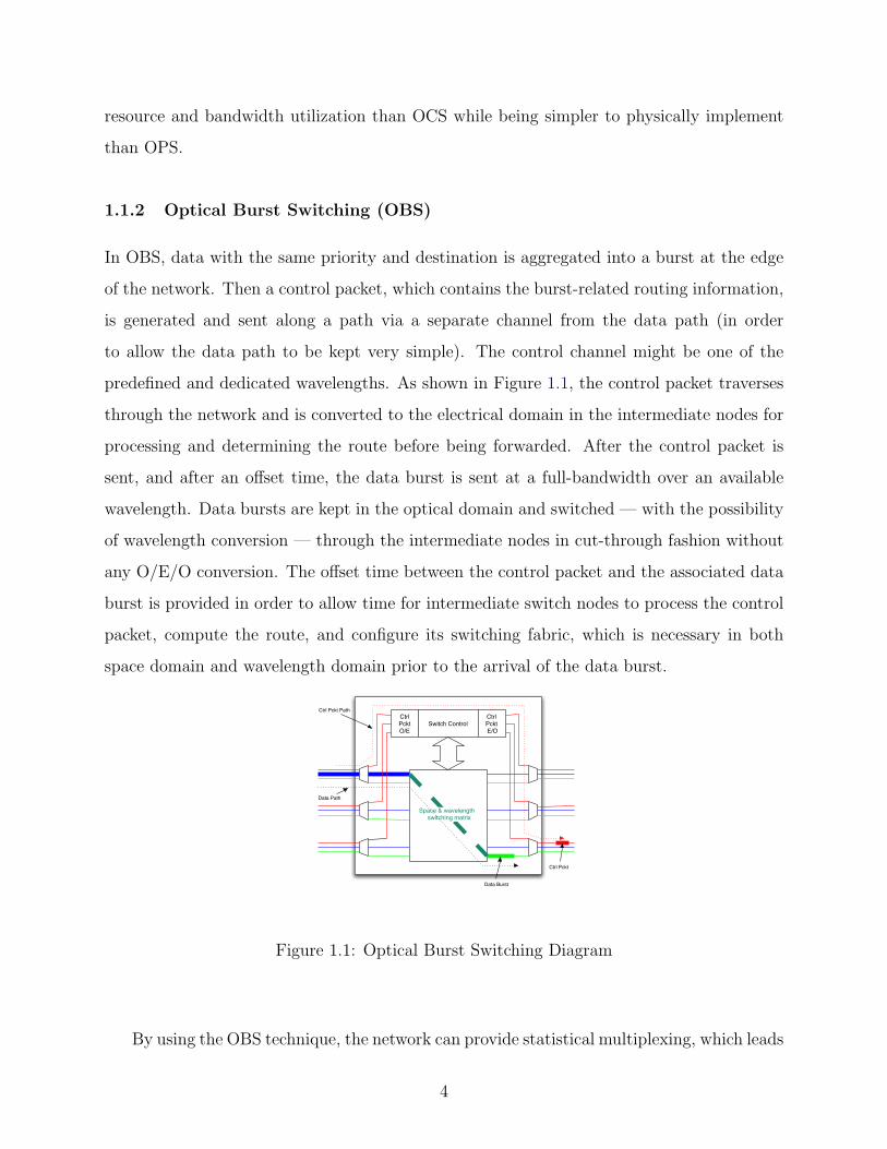
In OBS, data with the same priority and destination is aggregated into a burst at the edge
of the network. Then a control packet, which contains the burst-related routing information,
is generated and sent along a path via a separate channel from the data path (in order
to allow the data path to be kept very simple). The control channel might be one of the
predefined and dedicated wavelengths. As shown in Figure 1.1, the control packet traverses
through the network and is converted to the electrical domain in the intermediate nodes for
processing and determining the route before being forwarded. After the control packet is
sent, and after an offset time, the data burst is sent at a full-bandwidth over an available
wavelength. Data bursts are kept in the optical domain and switched — with the possibility
of wavelength conversion — through the intermediate nodes in cut-through fashion without
any O/E/O conversion. The offset time between the control packet and the associated data
burst is provided in order to allow time for intermediate switch nodes to process the control
packet, compute the route, and configure its switching fabric, which is necessary in both
space domain and wavelength domain prior to the arrival of the data burst.
Space & wavelength switching matrix
Switch ControlCtrl Pckt E/O
Ctrl PcktO/E
Ctrl Pckt Path
Ctrl Pckt
Data Burst
Data Path
Figure 1.1: Optical Burst Switching Diagram
By using the OBS technique, the network can provide statistical multiplexing, which leads
4
to better resource and bandwidth utilization than OCS in case of bursty traffic. Because
a wavelength is reserved only when there is a burst to transmit, and will be released when
the burst transmission finishes, the wavelength would be available for other transmissions.
In addition, OBS is considered to be an easier method to implement than OPS because of
following reasons.
• Since the control packet, which is converted to the electrical domain in intermediate
nodes, is sent via a separate channel, in-band complex optical processing (e.g. optical
extraction/insertion and realignment of the header in OPS) is avoided.
• Compared to the smaller size packets in the OPS, the core switching fabric reconfiguring
rate is lower since data is aggregated into a large burst before the transmission.
1.1.3 Design Issues for Optical Burst Switching
Since OBS works based on the all-optical switching techniques, the OBS protocol must
be carefully designed in order to efficiently support the unique characteristics of all-optical
switching. Several challenges are introduced due to the physical characteristic of all-optical
switches.
• First, a physical non-blocking all-optical switching fabric is currently constructed by
interconnecting small 2x2 switching devices to form larger switching fabric. Therefore
one factor, which contributes to the cost of implementing an all-optical switching fabric,
is the number of 2x2 switching devices required in the switching fabric. The cost of
implementing a fabric is correlated to this required number of 2x2 switching devices.
Therefore it is preferred that the design of an all-optical switching fabric should require
as few 2x2 switching devices as possible [10].
• Second, in the data burst transmission, since the number of wavelengths is limited,
contention in an OBS network can occur when one or more bursts needs a wavelength in
an outgoing port while no wavelength is available (currently reserved by other bursts).
As a result, bursts maybe blocked and then dropped. This occurrence should be minimal.
5
1.2 PROBLEM STATEMENT
The objective of this dissertation is to study recent technological aspects of Optical Burst
Switching (OBS) and to redesign the OBS protocol to balance between the cost of physical
implementation against system performance.
1.3 RESEARCH SUMMARY
The objective of this study is to review and identify the deficiencies of OBS protocols already
proposed, and to redesign the OBS protocol to balance the cost of physical implementation
against system performance. According to the review of the literature, we found out that
most of the proposed OBS protocols have variable burst size with non specific burst arrival
time. This leads to the requirement that a complex wide-sense non-blocking switching fabric
be implemented in OBS nodes in order to avoid any interruption while a data burst is
being transferred through the node. In addition, most of the proposed OBS protocols also
suffer from the situation in which a burst is partially blocked. This subsequently causes an
inefficient resource utilization of the available bandwidth in the network. More details of
these issues will be discussed in chapter 2 and 3.
The main contribution of this dissertation is the proposed variation of OBS protocols,
called Time-Synchronized OBS (SynOBS). SynOBS employs a synchronized timeslot-based
mechanism in order to allow a less complex rearrangeably non-blocking switching fabric to
be implemented, as well as to provide an opportunity to achieve better resource utilization
in the network compared to the previously proposed OBS protocols. The contributions of
this dissertation are summarized as follows:
• Design the basic protocol architecture and discuss a possible implementation of the basic
physical building blocks of SynOBS networks.
• Study the physical requirements of SynOBS and compare them to those of the previously
proposed OBSs, based on the number of physical 2x2 switching devices required in the
core switching fabric.
6
• Provide a mathematical model, which is used to estimate and analyze the performance
of SynOBS (in terms of burst loss probability) based on a given network configuration
and input traffic characteristics. This mathematical model will be used to analyze simple
models of SynOBS as well as to validate the SynOBS simulation model.
• Provide a SynOBS simulation model environment, which is used to analyze the model
of the SynOBS network, where the model is too complex for mathematical analysis.
• Study the effect of timeslot size on the performance of SynOBS and provide an analytical
framework for estimating the optimized solution based on a given network configuration
and input traffic characteristics. The effect of timeslot size is a trade-off between burst
assembly time and the guard time between consecutive timeslots (SynOBS works on a
fixed size timeslot mechanism).
• Study the implementation of optical buffers and its effect on system performance and
the physical requirements of SynOBS. In OBS, the optical signal is buffered in Fiber
Delay Lines (FDL). FDLa are used to delay those incoming bursts which are currently
blocked, so they can be switched out at a later time. While more FDLs available in an
OBS node means better blocking probability, additional FDL in a core node requires
additional physical requirements in core switching fabric.
Because OBS is based on all-optical switching, and since several areas in all-optical
switching are still emerging technologies, several assumptions have been made in this dis-
sertation in order to avoid existing unclear physical problems. The work is based on the
following assumptions, some of which are peripheral issues, some of which are discussed,
some simply assumed, but none of which are the core of the dissertation.
• The tunable wavelength converter for an all-optical network has received increasing at-
tention and is currently is an active area of research [10]. Several solutions were proposed
based on different technological approaches such as Optoelectronic Conversion (the com-
bination of photodetector and tunable laser), Optical Gating Wavelength Conversion,
and Wave-Mixing Wavelength Conversion. While each approach has its own character-
istics with different advantages and limitations, a winner among them is still unclear. In
order to maintain neutrality in this dissertation, it is assumed that the provided tunable
7
wavelength converters have full capability of wavelength conversion — which means, they
are able to convert any given input data wavelength to any output data wavelength.
• In current technology, wavelength conversion is expensive. This study proceeds under
the assumption that either (i) the cost will come down in the future, or (ii) architec-
tural techniques can be applied to reduce the number of converters (not part of this
dissertation).
• Since SynOBS employs a synchronized timeslot-based technique, the required mecha-
nism, which is used to realign and synchronize incoming data, is assumed to be available.
In this document, this mechanism is referred to as the timeslot synchronizer. While it is
not the main focus of this dissertation, some of the basic ideas for implementing such a
mechanism will be briefly studied and discussed.
• Since the all-optical switching fabric switches the data in an all optical domain, the data
is kept in this domain all the way to the destination, where it would encounter atten-
uation, dispersion, and timing variation. To keep the signal within acceptable quality,
therefore some forms of optical regeneration are required. The mechanism for providing
all optical regeneration is another current active research area. Such the examples of
optical regeneration mechanism are Erbium-Doped Fiber Amplifier (EDFA), Semicon-
ductor Laser Amplifier (SLA), SOA-MZI-Based 3R Regenerator, and Black-Box Optical
Regenerator (BBOR) [11]. While the mechanism for all optical regeneration is not in the
scope of this dissertation, it is assumed to be available.
• In SynOBS, It is possible for the data to be switched in space, wavelength, or time do-
main. While a large number of all-optical switching architectures have been proposed in
the area of all-optical switching (such as SLOB, KEOPS, WASPNET, and R. A. Thomp-
son and D. K. Hunter’s three-divisional architectures [12, 6, 13]), in this dissertation, the
switching architecture used is based on the separated time/space/wavelength switching
fabric which is the most widely adopted architecture for OBS [14, 15, 1, 16]. The detailed
description of the architecture is provided in sections 2.7 and 2.8.
8
1.4 OUTLINE
The remainder of this dissertation is organized as the following. Chapter 2 presents a back-
ground and review of the available literature in the field of OBS. Several variations of OBS
protocols are presented, as well as other concerned issues in OBS, including burst assembly,
physical implementation, and contention resolution in OBS. The objective is to provide the
reader an overview of the state-of-the-art in the field, and to identify the major concern
in designing an OBS system. The research problems raised in this chapter will be used to
propose a variation of synchronized timeslot-based OBS protocol (Time-Synchronized OBS)
in Chapter 3. Chapter 4 presents the performance analysis of Time-Synchronized OBS core
node, and the performance comparison between Time-Synchronized OBS and traditional
OBS. Then the analysis of the effect of timeslot size setting to the Time-Synchronized OBS
system is presented in Chapter 5. Chapter 6 discusses the algorithm/calculation for approx-
imating the optimized solution of the time size setting in Time-Synchronized OBS network
based on the lowest overall burst blocking probability. Finally, the conclusions of the dis-
sertation and the possible further researches for Time-Synchronized OBS are discussed in
Chapter 7.
9
2.0 BACKGROUND
2.1 OPTICAL BURST SWITCHING
OBS Network
Edge OBS Node
Core OBS Node
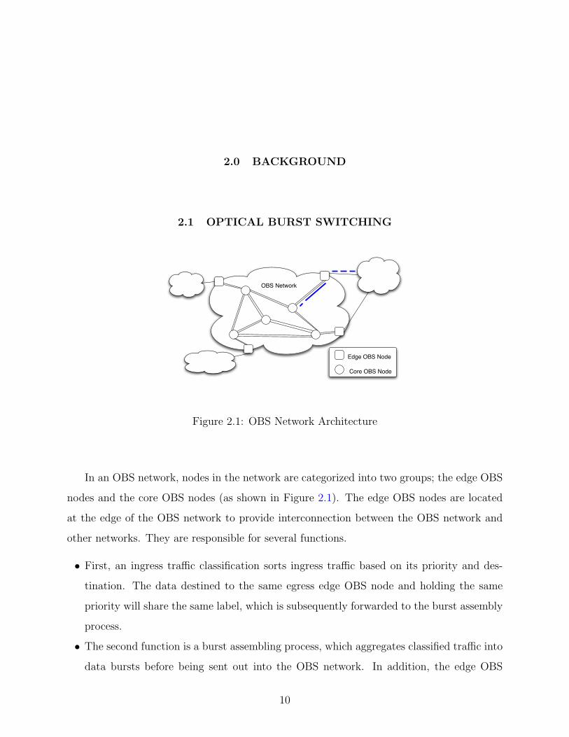
Figure 2.1: OBS Network Architecture
In an OBS network, nodes in the network are categorized into two groups; the edge OBS
nodes and the core OBS nodes (as shown in Figure 2.1). The edge OBS nodes are located
at the edge of the OBS network to provide interconnection between the OBS network and
other networks. They are responsible for several functions.
• First, an ingress traffic classification sorts ingress traffic based on its priority and des-
tination. The data destined to the same egress edge OBS node and holding the same
priority will share the same label, which is subsequently forwarded to the burst assembly
process.
• The second function is a burst assembling process, which aggregates classified traffic into
data bursts before being sent out into the OBS network. In addition, the edge OBS
10
node assigns a label to each data burst, generates the control packet which encapsulates
control and routing information along with the data burst, and forwards the control
packet and the data burst into the OBS network.
• Finally, the edge OBS nodes are also responsible for being egress nodes for data in the
OBS network, disassembling the burst, updating each data packet individually as needed,
and forwarding data packets out of the OBS network to their final destinations.
Core OBS nodes are core switch nodes in the OBS network. Their duty is to process
incoming control packets, determine routes, forward control packets based on given routing
information, and configure a switching matrix to switch the data burst to an outgoing port
based on the given routing information from the control packet.
2.2 ASYNCHRONOUS-BASED OBS
Many OBS protocol variations have been proposed. In this document, proposed OBS proto-
cols are divided into two categories. This section describes asynchronous-based OBS, which
has continuous variable data burst size. The next section describes timeslot-based OBS,
which has discrete variable burst size based on the duration of its timeslot.
Asynchronous-based OBS protocols assume that data bursts arrive asynchronously and
that burst size varies continuously. Two asynchronous-based protocols are described here
(e.g. Just-In-Time [17], Just-Enough-Time [18]).
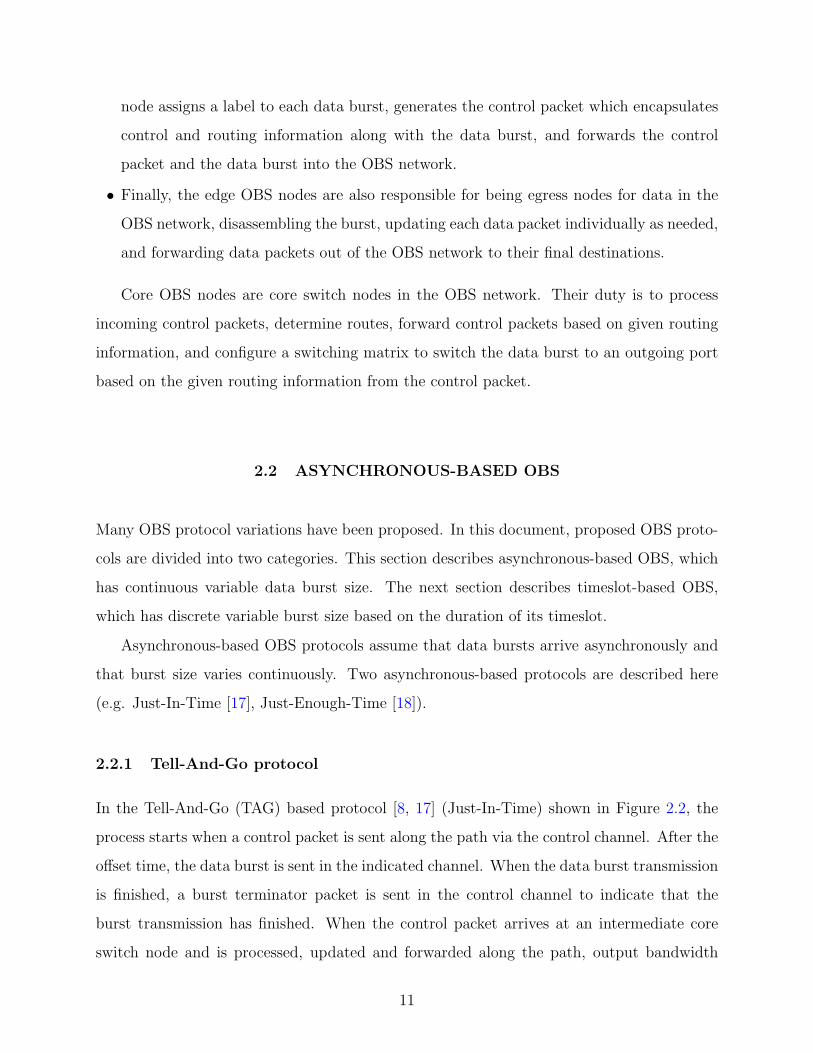
2.2.1 Tell-And-Go protocol
In the Tell-And-Go (TAG) based protocol [8, 17] (Just-In-Time) shown in Figure 2.2, the
process starts when a control packet is sent along the path via the control channel. After the
offset time, the data burst is sent in the indicated channel. When the data burst transmission
is finished, a burst terminator packet is sent in the control channel to indicate that the
burst transmission has finished. When the control packet arrives at an intermediate core
switch node and is processed, updated and forwarded along the path, output bandwidth
11
(wavelength and port) is reserved for the incoming data burst. While the data burst is
passing through the switch via the reserved outgoing wavelength/port, the switch waits for
the burst terminator packet from the control channel. After acquiring the burst terminator,
the output wavelength/port is released and is available for other transmissions. The burst
terminator is then forwarded along the outgoing path.
Control Pckt.
Data Burst
terminator
Control Channal
Data Channel
BW Reservation Time
Figure 2.2: Tell-And-Go Diagram
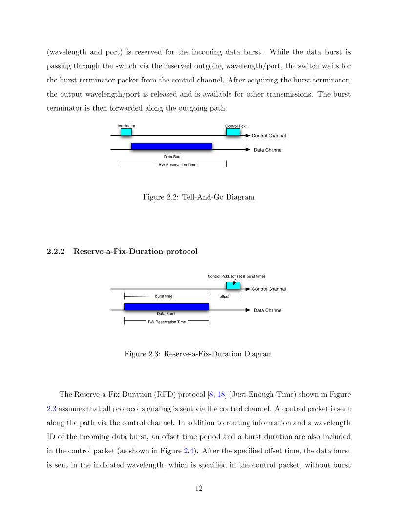
2.2.2 Reserve-a-Fix-Duration protocol
Control Pckt. (offset & burst time)
Data Burst
Control Channal
Data Channel
offsetburst time
BW Reservation Time
Figure 2.3: Reserve-a-Fix-Duration Diagram
The Reserve-a-Fix-Duration (RFD) protocol [8, 18] (Just-Enough-Time) shown in Figure
2.3 assumes that all protocol signaling is sent via the control channel. A control packet is sent
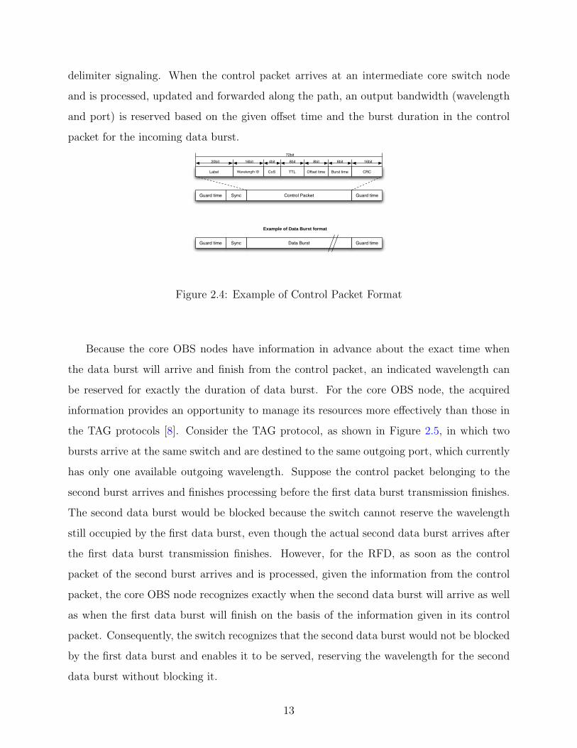
along the path via the control channel. In addition to routing information and a wavelength
ID of the incoming data burst, an offset time period and a burst duration are also included
in the control packet (as shown in Figure 2.4). After the specified offset time, the data burst
is sent in the indicated wavelength, which is specified in the control packet, without burst
12
delimiter signaling. When the control packet arrives at an intermediate core switch node
and is processed, updated and forwarded along the path, an output bandwidth (wavelength
and port) is reserved based on the given offset time and the burst duration in the control
packet for the incoming data burst.
Control PacketSyncGuard time
CoSWavelength ID Offset timeLabel Burst time CRCTTL
20bit 16bit16bit 8bit8bit8bit4bit
Guard time
Data BurstSyncGuard time Guard time
72bit
Example of Data Burst format
Figure 2.4: Example of Control Packet Format
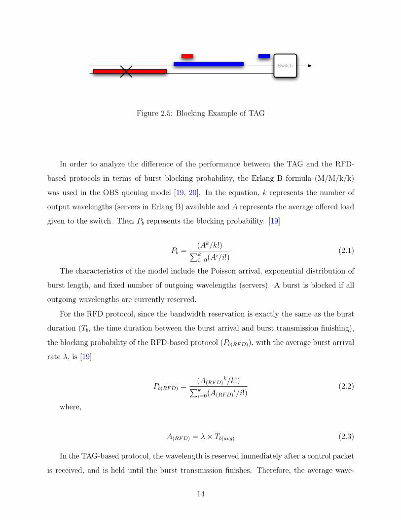
Because the core OBS nodes have information in advance about the exact time when
the data burst will arrive and finish from the control packet, an indicated wavelength can
be reserved for exactly the duration of data burst. For the core OBS node, the acquired
information provides an opportunity to manage its resources more effectively than those in
the TAG protocols [8]. Consider the TAG protocol, as shown in Figure 2.5, in which two
bursts arrive at the same switch and are destined to the same outgoing port, which currently
has only one available outgoing wavelength. Suppose the control packet belonging to the
second burst arrives and finishes processing before the first data burst transmission finishes.
The second data burst would be blocked because the switch cannot reserve the wavelength
still occupied by the first data burst, even though the actual second data burst arrives after
the first data burst transmission finishes. However, for the RFD, as soon as the control
packet of the second burst arrives and is processed, given the information from the control
packet, the core OBS node recognizes exactly when the second data burst will arrive as well
as when the first data burst will finish on the basis of the information given in its control
packet. Consequently, the switch recognizes that the second data burst would not be blocked
by the first data burst and enables it to be served, reserving the wavelength for the second
data burst without blocking it.
13
Switch
Figure 2.5: Blocking Example of TAG
In order to analyze the difference of the performance between the TAG and the RFD-
based protocols in terms of burst blocking probability, the Erlang B formula (M/M/k/k)
was used in the OBS queuing model [19, 20]. In the equation, k represents the number of
output wavelengths (servers in Erlang B) available and A represents the average offered load
given to the switch. Then Pb represents the blocking probability. [19]
Pb =(Ak/k!)∑ki=0(A
i/i!)(2.1)
The characteristics of the model include the Poisson arrival, exponential distribution of
burst length, and fixed number of outgoing wavelengths (servers). A burst is blocked if all
outgoing wavelengths are currently reserved.
For the RFD protocol, since the bandwidth reservation is exactly the same as the burst
duration (Tb, the time duration between the burst arrival and burst transmission finishing),
the blocking probability of the RFD-based protocol (Pb(RFD)), with the average burst arrival
rate λ, is [19]
Pb(RFD) =(A(RFD)
k/k!)∑ki=0(A(RFD)
i/i!)(2.2)
where,
A(RFD) = λ× Tb(avg) (2.3)
In the TAG-based protocol, the wavelength is reserved immediately after a control packet
is received, and is held until the burst transmission finishes. Therefore, the average wave-
14
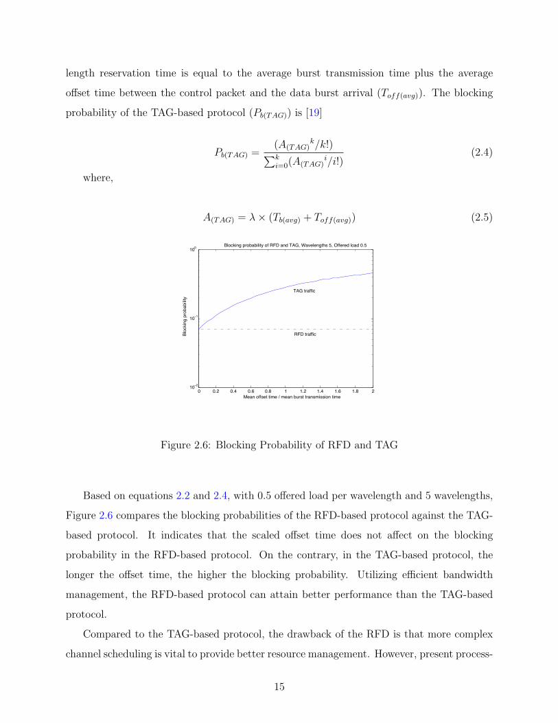
length reservation time is equal to the average burst transmission time plus the average
offset time between the control packet and the data burst arrival (Toff(avg)). The blocking
probability of the TAG-based protocol (Pb(TAG)) is [19]
Pb(TAG) =(A(TAG)
k/k!)∑ki=0(A(TAG)
i/i!)(2.4)
where,
A(TAG) = λ× (Tb(avg) + Toff(avg)) (2.5)
0 0.2 0.4 0.6 0.8 1 1.2 1.4 1.6 1.8 210
!2
10!1
100
Blocking probability of RFD and TAG, Wavelengths 5, Offered load 0.5
Mean offset time / mean burst transmission time
Blo
ckin
g p
rob
ab
ility
RFD traffic
TAG traffic
Figure 2.6: Blocking Probability of RFD and TAG
Based on equations 2.2 and 2.4, with 0.5 offered load per wavelength and 5 wavelengths,
Figure 2.6 compares the blocking probabilities of the RFD-based protocol against the TAG-
based protocol. It indicates that the scaled offset time does not affect on the blocking
probability in the RFD-based protocol. On the contrary, in the TAG-based protocol, the
longer the offset time, the higher the blocking probability. Utilizing efficient bandwidth
management, the RFD-based protocol can attain better performance than the TAG-based
protocol.
Compared to the TAG-based protocol, the drawback of the RFD is that more complex
channel scheduling is vital to provide better resource management. However, present process-
15
ing power enables handling the complex channel scheduling introduced by the RFD-based
protocol [8], thus suggesting the use of the RFD-based protocol as the protocol solution for
OBS networks.
2.3 TIMESLOT-BASED OBS
Among those proposed OBS protocol variations, asynchronous OBS protocols were extended
to synchronous timeslot-based OBS. In timeslot-based OBS, the data channel is divided into
timeslots. Incoming data streams from different input ports must be realigned to the slot
boundaries to maintain synchronization prior to entering the switching fabric. One of the
advantages of timeslot-based OBS is that it allows a burst to be reserved on a timeslot basis
instead of unpredictable continuous time as in asynchronous-based OBS. Thus, this should
allow a more predictable/manageable switching schedule, and should reduce the complexity
of wavelength reservation processing.
2.3.1 Time Sliced OBS protocol
Contents in adata burst
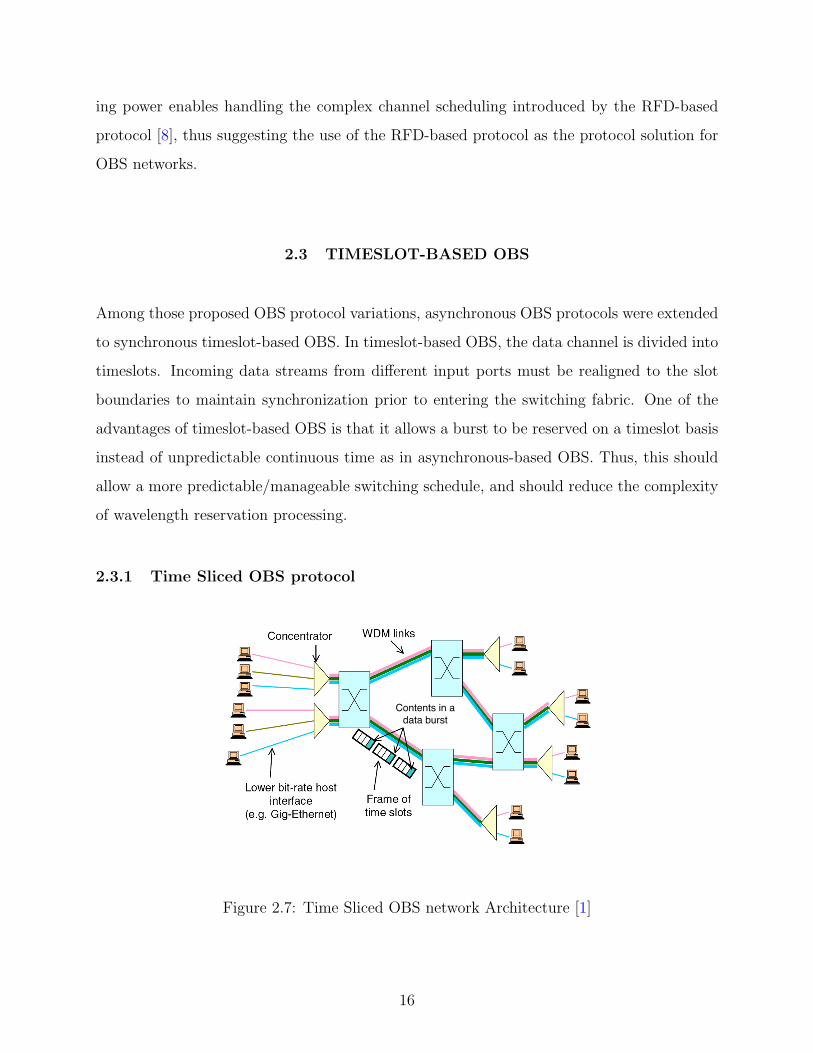
Figure 2.7: Time Sliced OBS network Architecture [1]
16
One of proposed variants of timeslot-based OBS is Time Sliced Optical Burst Switching
(TSOBS) [1] shown in Figure 2.7, which replaces switching in the wavelength domain with
switching in the time domain. Like traditional optical burst switching, TSOBS separates
burst control information from burst data. Specifically, Control packets are transmitted on
dedicated control wavelengths on outgoing links. This wavelength is converted to the electri-
cal domain at each intermediate node for control packet processing, while all other remaining
data wavelengths are kept in the optical domain and switched through each intermediate
node in optical form.
With Optical Time Slot Interchangers (OTSI), Time-Division Multiplexing (TDM) is
used in TSOBS to carry information as well as to resolve the contention resolution in the
data wavelength. The data stream consists of a repeating frame structure which is sub-
divided into fixed-size timeslots. The repeating sequence of timeslots at a fixed position
within successive frames is called as a channel. The information carried in the control
packet consist of destination address information, the incoming data wavelength, the data
channel used by the arriving data burst, the offset information, and the length of the data
burst. The offset information identifies the frame in which the data channel starts containing
the data, and the length identifies the number of frames in which the data channel is used
by the arriving burst.
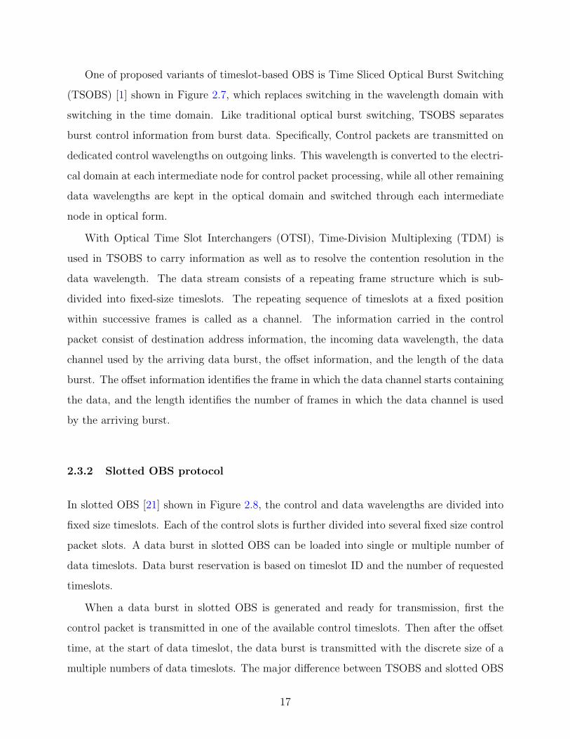
2.3.2 Slotted OBS protocol
In slotted OBS [21] shown in Figure 2.8, the control and data wavelengths are divided into
fixed size timeslots. Each of the control slots is further divided into several fixed size control
packet slots. A data burst in slotted OBS can be loaded into single or multiple number of
data timeslots. Data burst reservation is based on timeslot ID and the number of requested
timeslots.
When a data burst in slotted OBS is generated and ready for transmission, first the
control packet is transmitted in one of the available control timeslots. Then after the offset
time, at the start of data timeslot, the data burst is transmitted with the discrete size of a
multiple numbers of data timeslots. The major difference between TSOBS and slotted OBS
17
Core Switching
Fabric
Slotted OBS node
time slot alignmentsburst 2
burst 1
burst 2
burst 1burst 1
Figure 2.8: Example of Slotted OBS
is that, TSOBS is based on TDM channeling to carry information in data wavelength and
assumes that there is no wavelength conversion in any intermediate nodes. On the contrary,
slotted OBS assumes that wavelength conversion in the intermediate nodes is possible.
2.4 OFFSET TIME MANAGEMENT
Offset time is the time duration between the start of the control packet transmission and
the start of the data burst transmission. It is used for allowing the control packet to be
processed in an intermediate node before the data burst arrives.
Each time a control packet passes an intermediate node, it is converted to the electrical
domain, stored, and processed before being updated and forwarded to the next node. This
processing causes a delay at the intermediate node. On the other hand, the data burst simply
cuts through the intermediate node without any delay. Therefore, each time a control packet
and a data burst pass through an intermediate node, the offset time decreases because of
the control packet processing delay, as shown in Figure 2.9. If the RFD protocol has been
applied, the offset time field in the control packet must be updated in every intermediate
node.
18
OBS Time Diagram
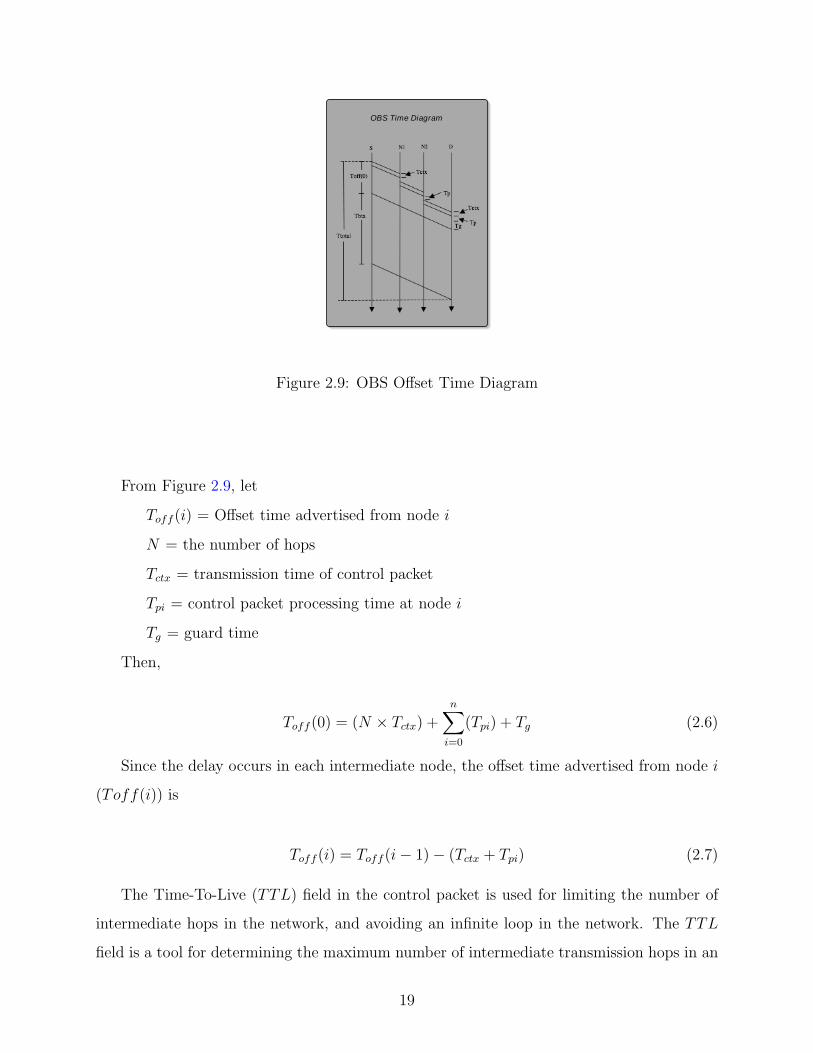
Figure 2.9: OBS Offset Time Diagram
From Figure 2.9, let
Toff (i) = Offset time advertised from node i
N = the number of hops
Tctx = transmission time of control packet
Tpi = control packet processing time at node i
Tg = guard time
Then,
Toff (0) = (N × Tctx) +n∑i=0
(Tpi) + Tg (2.6)
Since the delay occurs in each intermediate node, the offset time advertised from node i
(Toff(i)) is
Toff (i) = Toff (i− 1)− (Tctx + Tpi) (2.7)
The Time-To-Live (TTL) field in the control packet is used for limiting the number of
intermediate hops in the network, and avoiding an infinite loop in the network. The TTL
field is a tool for determining the maximum number of intermediate transmission hops in an
19
OBS network. Therefore,
Toff (0) = (TTL× (Tctx + T̄p)) + Tg (2.8)
Where, T̄p = Average processing time in every node
2.5 QOS AND PRIORITIES
To support various types of service —voice, data, video, etc.— in the next generation net-
works, Quality of Service (QoS) support in core networks is inevitable. Because of the lack
of optical buffers, existing priority schemes no longer apply to OBS. Therefore, a new mecha-
nism has been proposed to support different QoS priorities in the RFD-based OBS protocol.
Bursts are classified into multiple classes, and the differentiation of a class burst priority
is based on the probability of a blocked burst —the higher priority class burst has a lower
probability of being blocked.
2.5.1 Offset Time Management for Supporting QoS and Priorities
The main idea for providing class differentiation is based on providing more offset time for
the higher priority bursts [22, 20]. A control packet that reaches an intermediate node first
has the right to reserve the output wavelength first. Therefore, the longer the offset time,
the higher the probability of successfully reserving wavelength. The longer offset time allows
the wavelength of the data burst to be reserved earlier.
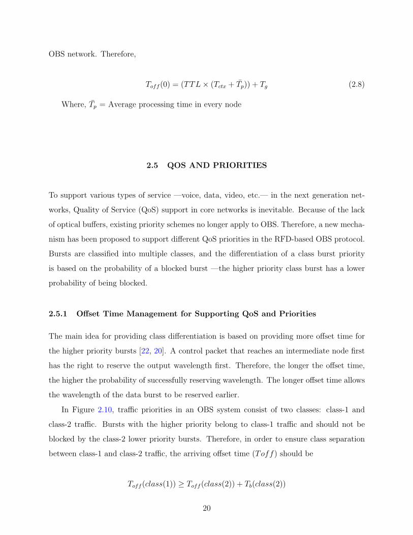
In Figure 2.10, traffic priorities in an OBS system consist of two classes: class-1 and
class-2 traffic. Bursts with the higher priority belong to class-1 traffic and should not be
blocked by the class-2 lower priority bursts. Therefore, in order to ensure class separation
between class-1 and class-2 traffic, the arriving offset time (Toff) should be
Toff (class(1)) ≥ Toff (class(2)) + Tb(class(2))
20
Switch
Class 1 Toff
Class 2 ToffClass 2 Tb
* class 1 has higher priority than class 2
Figure 2.10: OBS Offset Time with QoS Diagram
As we can see from Figure 2.10, if the above condition is satisfied, then it is unlikely that
a class-1 burst is blocked by a class-2 burst. When a control packet of a class-1 burst arrives,
the output wavelength is reserved for the class-1 data burst without any blocking from the
class-2 burst because all the currently reserved class-2 bursts will have finished before the
arrival of the class-1 data burst. On the contrary, a class-2 burst tends to be blocked by
a class-1 burst because, by the time the control packet of the class-2 burst arrives, with
its shorter offset time, the output wavelength has already been reserved by the previously
arriving class-1 control packet. Therefore, if the traffic consists of N classes, where the class-
1 has the highest priority and the class-N has the lowest priority, according to the above
discussion
Toff (class(i)) ≥ Toff (class(i+ 1)) + Tb(class(i+ 1)) (2.9)
Toff (a, b) represents an offset time of class b burst advertised from node a.
This is combined with utilizing the TTL field for limiting the maximum number of
intermediate hops in the OBS network, this combination is summarized in the equation:
Toff (0, i) = [TTL× (Tctx + T̄p) + Tg] + [Tb + Toff (0, i+ 1)]
Toff (0, N) = [TTL× (Tctx + T̄p) + Tg] (2.10)
21

Toff (0, i) = [(N − i+ 1)× (TTL× (Tctx + T̄p) + Tg)] + [Tb × (N − i)] (2.11)
According the above QoS mechanism, the higher priority means longer delay, because
longer offset times cause the data burst to wait in the edge OBS node for its offset time
period before the burst can be sent out. Normally these high priority bursts may belong
to the traffic that is sensitive to overall delay performance, such as interactive applications
and voice. However, the mechanism is based on the assumption that the line speed of each
wavelength is considerably high (e.g. 10 Gbps) when compared to the average burst size.
Continuing, if the size of the control packets is 1000 bytes, Then Tctx = 0.8 usec. In addition,
assume that Tp is 0.8 usec (same as Tctx) that the average burst size is 1 Mbyte, causing Tb
≈ 0.8 msec, and that the guard time is 5 times of Tctx, which is 4 usec. Suppose there are 5
QoS classes and TTL = 10, then from (2.11), the offset time delay for the highest priority
class-1 is around 3.48 msec. However, a delay of one extra offset time is not significant to
most delay sensible applications (≈ 30 msec for voice). Therefore, it is likely that the extra
offset time caused by the mechanism would have little affect on overall delay performance.
2.6 BURST ASSEMBLY
In an OBS network, data is transmitted in the form of a burst. Incoming data (e.g. IP
packets) is assembled to form a data burst at the ingress edge OBS node before it is sent
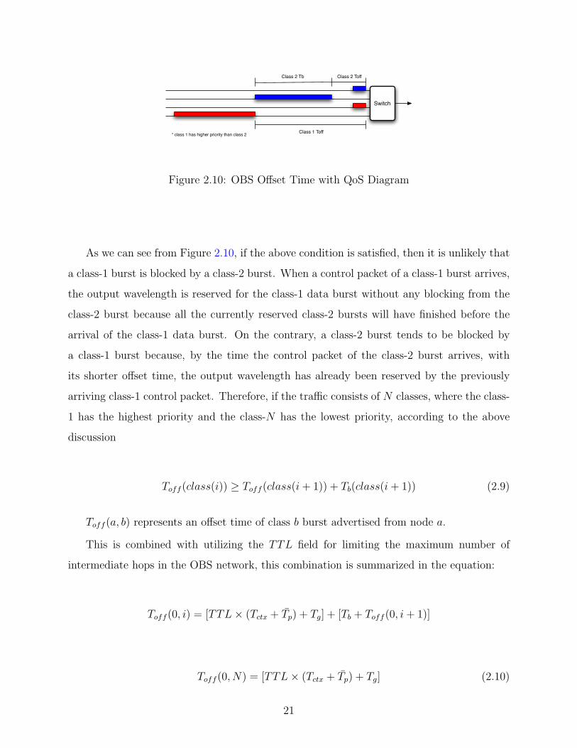
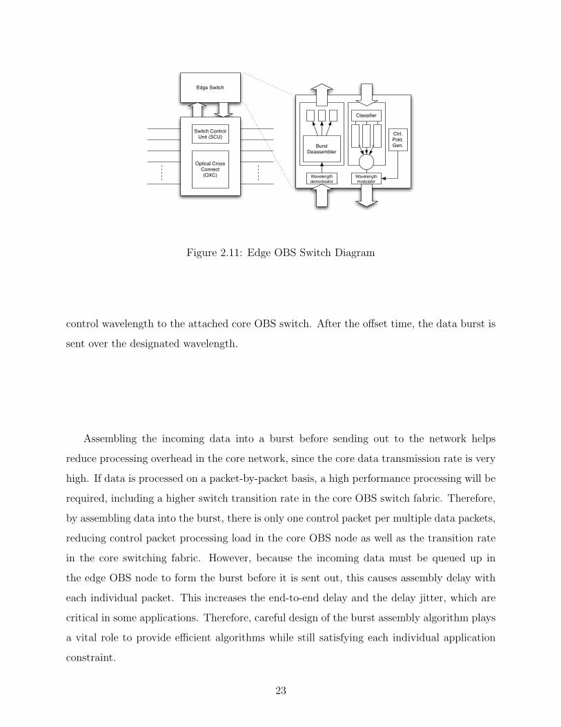
into the OBS network. Figure 2.11 demonstrates a simple architecture of an edge OBS node.
When ingress traffic arrives at the edge OBS node, the traffic first passes through a classifier.
The classifier is responsible for classifying incoming traffic based on its priority and its egress
edge OBS node. Then, the classifier forwards the classified traffic to an appropriate queue,
based on the type of data priority and the destination edge OBS node. The traffic with the
same priority and destination is queued up and assembled together to form the data burst in
the queue. As soon as the data burst is ready, a control packet is generated and sent via the
22
Switch Control Unit (SCU)
Optical Cross Connect (OXC)
Edge Switch
Classifier
Wavelength demodulator
Burst Deassembler
Ctrl. Pckt. Gen.
Wavelength modulator
Figure 2.11: Edge OBS Switch Diagram
control wavelength to the attached core OBS switch. After the offset time, the data burst is
sent over the designated wavelength.
Assembling the incoming data into a burst before sending out to the network helps
reduce processing overhead in the core network, since the core data transmission rate is very
high. If data is processed on a packet-by-packet basis, a high performance processing will be
required, including a higher switch transition rate in the core OBS switch fabric. Therefore,
by assembling data into the burst, there is only one control packet per multiple data packets,
reducing control packet processing load in the core OBS node as well as the transition rate
in the core switching fabric. However, because the incoming data must be queued up in
the edge OBS node to form the burst before it is sent out, this causes assembly delay with
each individual packet. This increases the end-to-end delay and the delay jitter, which are
critical in some applications. Therefore, careful design of the burst assembly algorithm plays
a vital role to provide efficient algorithms while still satisfying each individual application
constraint.
23
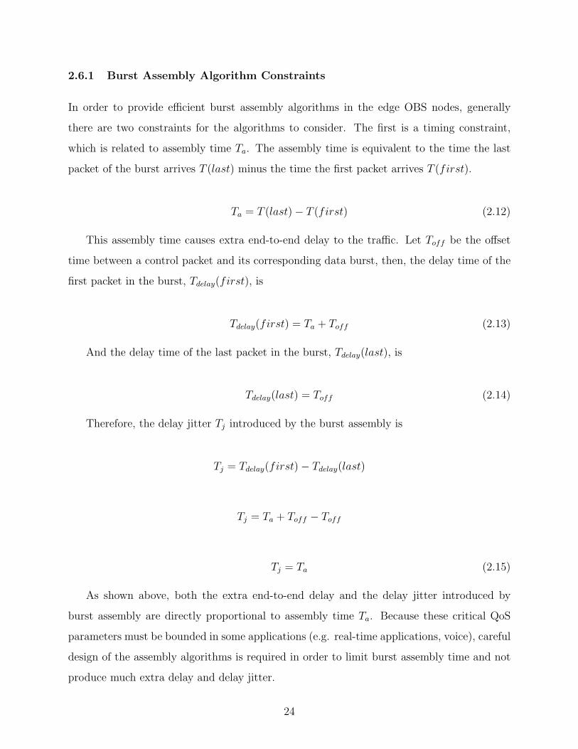
2.6.1 Burst Assembly Algorithm Constraints
In order to provide efficient burst assembly algorithms in the edge OBS nodes, generally
there are two constraints for the algorithms to consider. The first is a timing constraint,
which is related to assembly time Ta. The assembly time is equivalent to the time the last
packet of the burst arrives T (last) minus the time the first packet arrives T (first).
Ta = T (last)− T (first) (2.12)
This assembly time causes extra end-to-end delay to the traffic. Let Toff be the offset
time between a control packet and its corresponding data burst, then, the delay time of the
first packet in the burst, Tdelay(first), is
Tdelay(first) = Ta + Toff (2.13)
And the delay time of the last packet in the burst, Tdelay(last), is
Tdelay(last) = Toff (2.14)
Therefore, the delay jitter Tj introduced by the burst assembly is
Tj = Tdelay(first)− Tdelay(last)
Tj = Ta + Toff − Toff
Tj = Ta (2.15)
As shown above, both the extra end-to-end delay and the delay jitter introduced by
burst assembly are directly proportional to assembly time Ta. Because these critical QoS
parameters must be bounded in some applications (e.g. real-time applications, voice), careful
design of the assembly algorithms is required in order to limit burst assembly time and not
produce much extra delay and delay jitter.
24
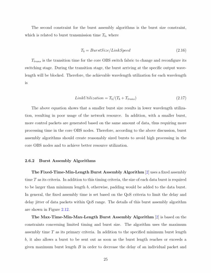
The second constraint for the burst assembly algorithms is the burst size constraint,
which is related to burst transmission time Tb, where
Tb = BurstSize/LinkSpeed (2.16)
Ttrans is the transition time for the core OBS switch fabric to change and reconfigure its
switching stage. During the transition stage, the burst arriving at the specific output wave-
length will be blocked. Therefore, the achievable wavelength utilization for each wavelength
is
LinkUtilization = Tb/(Tb + Ttrans) (2.17)
The above equation shows that a smaller burst size results in lower wavelength utiliza-
tion, resulting in poor usage of the network resource. In addition, with a smaller burst,
more control packets are generated based on the same amount of data, thus requiring more
processing time in the core OBS nodes. Therefore, according to the above discussion, burst
assembly algorithms should create reasonably sized bursts to avoid high processing in the
core OBS nodes and to achieve better resource utilization.
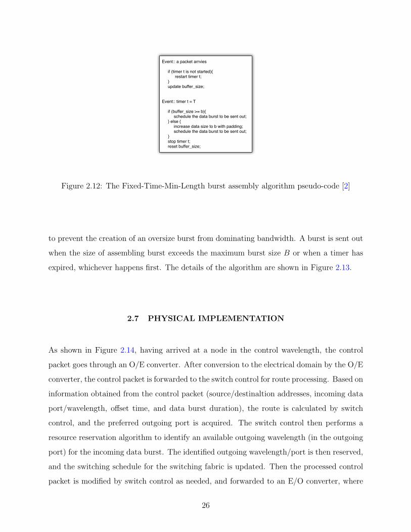
2.6.2 Burst Assembly Algorithms
The Fixed-Time-Min-Length Burst Assembly Algorithm [2] uses a fixed assembly
time T as its criteria. In addition to this timing criteria, the size of each data burst is required
to be larger than minimum length b, otherwise, padding would be added to the data burst.
In general, the fixed assembly time is set based on the QoS criteria to limit the delay and
delay jitter of data packets within QoS range. The details of this burst assembly algorithm
are shown in Figure 2.12.
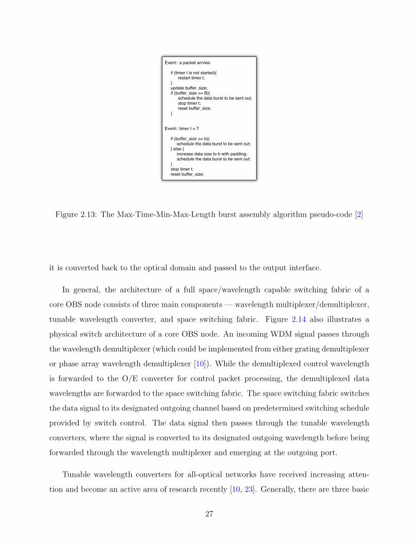
The Max-Time-Min-Max-Length Burst Assembly Algorithm [2] is based on the
constraints concerning limited timing and burst size. The algorithm uses the maximum
assembly time T as its primary criteria. In addition to the specified minimum burst length
b, it also allows a burst to be sent out as soon as the burst length reaches or exceeds a
given maximum burst length B in order to decrease the delay of an individual packet and
25
Event:: a packet arrvies
if (timer t is not started){ restart timer t; } update buffer_size;
Event:: timer t = T
if (buffer_size >= b){ schedule the data burst to be sent out; } else { increase data size to b with padding; schedule the data burst to be sent out; } stop timer t; reset buffer_size;
Figure 2.12: The Fixed-Time-Min-Length burst assembly algorithm pseudo-code [2]
to prevent the creation of an oversize burst from dominating bandwidth. A burst is sent out
when the size of assembling burst exceeds the maximum burst size B or when a timer has
expired, whichever happens first. The details of the algorithm are shown in Figure 2.13.
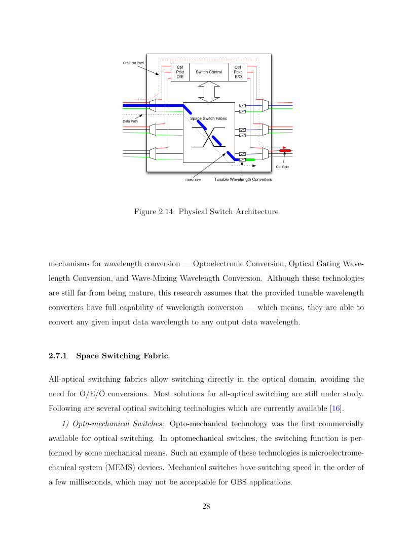
2.7 PHYSICAL IMPLEMENTATION
As shown in Figure 2.14, having arrived at a node in the control wavelength, the control
packet goes through an O/E converter. After conversion to the electrical domain by the O/E
converter, the control packet is forwarded to the switch control for route processing. Based on
information obtained from the control packet (source/destinaltion addresses, incoming data
port/wavelength, offset time, and data burst duration), the route is calculated by switch
control, and the preferred outgoing port is acquired. The switch control then performs a
resource reservation algorithm to identify an available outgoing wavelength (in the outgoing
port) for the incoming data burst. The identified outgoing wavelength/port is then reserved,
and the switching schedule for the switching fabric is updated. Then the processed control
packet is modified by switch control as needed, and forwarded to an E/O converter, where
26
Event:: a packet arrvies
if (timer t is not started){ restart timer t; } update buffer_size; if (buffer_size >= B){ schedule the data burst to be sent out; stop timer t; reset buffer_size; }
Event:: timer t = T
if (buffer_size >= b){ schedule the data burst to be sent out; } else { increase data size to b with padding; schedule the data burst to be sent out; } stop timer t; reset buffer_size;
Figure 2.13: The Max-Time-Min-Max-Length burst assembly algorithm pseudo-code [2]
it is converted back to the optical domain and passed to the output interface.
In general, the architecture of a full space/wavelength capable switching fabric of a
core OBS node consists of three main components — wavelength multiplexer/demultiplexer,
tunable wavelength converter, and space switching fabric. Figure 2.14 also illustrates a
physical switch architecture of a core OBS node. An incoming WDM signal passes through
the wavelength demultiplexer (which could be implemented from either grating demultiplexer
or phase array wavelength demultiplexer [10]). While the demultiplexed control wavelength
is forwarded to the O/E converter for control packet processing, the demultiplexed data
wavelengths are forwarded to the space switching fabric. The space switching fabric switches
the data signal to its designated outgoing channel based on predetermined switching schedule
provided by switch control. The data signal then passes through the tunable wavelength
converters, where the signal is converted to its designated outgoing wavelength before being
forwarded through the wavelength multiplexer and emerging at the outgoing port.
Tunable wavelength converters for all-optical networks have received increasing atten-
tion and become an active area of research recently [10, 23]. Generally, there are three basic
27
Switch ControlCtrl Pckt E/O
Ctrl PcktO/E
Ctrl Pckt Path
Ctrl Pckt
Data Burst
Data PathSpace Switch Fabric
Tunable Wavelength Converters
Figure 2.14: Physical Switch Architecture
mechanisms for wavelength conversion — Optoelectronic Conversion, Optical Gating Wave-
length Conversion, and Wave-Mixing Wavelength Conversion. Although these technologies
are still far from being mature, this research assumes that the provided tunable wavelength
converters have full capability of wavelength conversion — which means, they are able to
convert any given input data wavelength to any output data wavelength.
2.7.1 Space Switching Fabric
All-optical switching fabrics allow switching directly in the optical domain, avoiding the
need for O/E/O conversions. Most solutions for all-optical switching are still under study.
Following are several optical switching technologies which are currently available [16].
1) Opto-mechanical Switches: Opto-mechanical technology was the first commercially
available for optical switching. In optomechanical switches, the switching function is per-
formed by some mechanical means. Such an example of these technologies is microelectrome-
chanical system (MEMS) devices. Mechanical switches have switching speed in the order of
a few milliseconds, which may not be acceptable for OBS applications.
28
2) Electro-optic Switches: A 2x2 electrooptic switch uses a directional coupler whose
coupling ratio is changed by varying the refractive index of the material in the coupling
region. One commonly used material is lithium niobate (LiNbO3). A switch is constructed
on a lithium niobate waveguide. An electrical voltage applied to the electrodes changes
the substrate’s index of refraction. The change in the index of refraction manipulates the
light through the appropriate waveguide path to the desired port. An electrooptic switch
is capable of changing its state extremely rapidly, typically in less than a nanosecond. This
switching time limit is determined by the capacitance of the electrode configuration. Larger
switches can be constructed by integrating several 2x2 switches on a single substrate.
3) Thermo-optic Switches: The operation of these devices is based on the thermo-optic
effect. It consists in the variation of the refractive index of a dielectric material, due to
temperature variation of the material itself.
4) Semiconductor Optical Amplifier Switches: Semiconductor optical amplifiers (SOAs)
are versatile devices that are used for many purposes in optical networks. An SOA can be
used as an ON-OFF switch by varying the bias voltage. If the bias voltage is reduced, no
population inversion is achieved, and the device absorbs input signals. If the bias voltage
is present, it amplifies the input signals. Larger switches can be fabricated by integrating
SOAs with passive couplers.
2.7.1.1 Switching Fabric Constraints To design a large space switching fabric, there
are several factors affecting overall implementation cost and performance, which have to be
taken into account. These factors are the following [10].
1) Switching time: One of the most important factors to be considered for switching
fabrics is switching time. Switching time is the time a switch needs for changing its switching
state. Different switching technologies have different switching time varying from an order of
few milliseconds (MEMS) to less than a nanosecond (Lithium Niobate Switched Directional
Coupler). Different applications have different switching time requirements.
2) Crosstalk: Crosstalk is an undesired leakage of an attenuated version of the signal that
emerges at the unintended outgoing port. It is the ratio of the power at a specific output
port from its intended input port to the power from all other input ports.
29
3) Loss Uniformity: A switching fabric may have different losses for different combi-
nations of input and output ports. This situation might become more significant in larger
switching fabrics. The measure of loss uniformity might be obtained by considering the
minimum and maximum number of 2x2 switching devices in the optical path, for different
input and output combinations. It is preferred that these numbers should vary as little as
possible.
4) Number of 2x2 switching devices required: Because large optical switching fabrics are
made by interconnecting a number of 2x2 switching devices together, and that the cost of
implementing switching fabrics is correlated to the number of 2x2 switching devices required.
Therefore it is preferred that the design of large switching fabric should require as few 2x2
switching devices as possible.
5) Number of Crossovers: Large switching fabrics are sometimes fabricated by integrating
2x2 switching devices on a single substrate (e.g. lithium niobate directional coupler switches
[23]). Unlike integrated electronic circuits (ICs), where various components are made at
multiple layers in which those interconnections between layers are possible, in integrated
optics all these interconnections must be made in a single layer by means of waveguides.
If these interconnection paths are crossed, power loss and crosstalk might be introduced.
Therefore it is desirable that crossed interconnection paths are minimized, or completely
eliminated.
6) Blocking Characteristic: Normally switching fabrics function are categorized into two
types — nonblocking and blocking. A switch is said to be nonblocking if an unused input
port can be connected to any unused output port; otherwise, it is said to be blocking. In
the application of OBS, a nonblocking switch is normally required. However, nonblocking
switching fabrics are further categorized based on their properties. A switch is said to
be wide-sense nonblocking if any unused input can be connected to any unused output,
without requiring any existing connections to be rerouted. On the contrary, a switch is
said to be rearrangeably nonblocking if any unused input can be connected to any unused
output, but may require some (or all) of its existing connections to be rerouted. Normally,
while rearrangeably nonblocking architectures require fewer 2x2 switching devices, the main
drawback of rearrangeably nonblocking architecture is that many applications will not allow
30
existing connections to be disrupted to accommodate a new connection. Such an example
of these applications are the OBS protocols previously discussed in section 2.2 due to their
nature of their asynchronous burst arrival and variable burst size.
V bar V cross
Figure 2.15: LiNbO3 Switched Directional Coupler
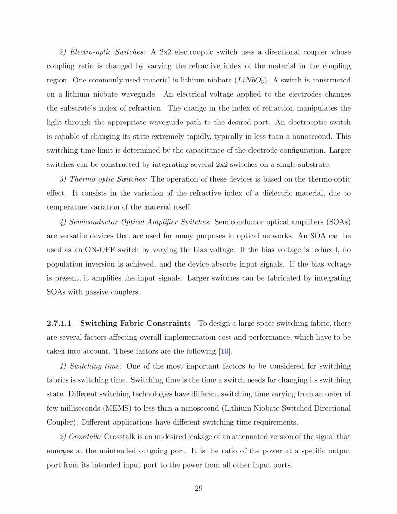
2.7.1.2 Examples of Switching Fabric Architecture An optical space switching fab-
ric can be implemented by interconnecting fast 2x2 switching devices (the beta element) to
form a larger fabric. Such an example of the 2x2 switching device is Lithium Niobate
Switched Directional Coupler (SDC) [23]. Based on the voltage applied to the SDC, the
switch can be set to either the BAR state or the CROSS state as shown in Figure 2.15, the
BAR state represents the state in which the signals emerge from output ports on the same
physical channel as their respective input ports, and the CROSS state represents the state
in which the input signals cross over to their opposite physical channels. Following are some
of the examples of switching fabric architecture:
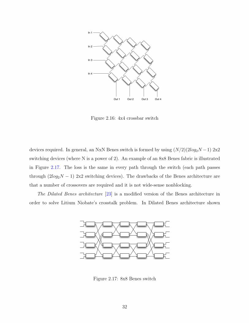
The crossbar architecture [10] is an example of wide-sense nonblocking architecture. In
general, an NxN crossbar is formed by using N2 2x2 switching devices. Figure 2.16 illustrates
an example of 4x4 crossbar switch. Generally, to connect input i to output j, the path taken
traverses the 2x2 switching devices in row i until it reaches column j, and then traverses
the 2x2 switching devices in column j until it reaches output j. One of the advantages of
a crossbar is that there are no crossovers in the architecture. However, loss uniformity (for
NxN crossbar, the shortest path length is 1 and the longest path is 2N − 1), is one of the
main drawbacks of this architecture.
The Benes architecture [10, 23] is a rearrangeably nonblocking architecture. It is one
of the most efficient switching fabric architecture in terms of the number of 2x2 switching
31
In 1
In 4
In 3
In 2
Out 1 Out 4Out 3Out 2
Figure 2.16: 4x4 crossbar switch
devices required. In general, an NxN Benes switch is formed by using (N/2)(2log2N−1) 2x2
switching devices (where N is a power of 2). An example of an 8x8 Benes fabric is illustrated
in Figure 2.17. The loss is the same in every path through the switch (each path passes
through (2log2N − 1) 2x2 switching devices). The drawbacks of the Benes architecture are
that a number of crossovers are required and it is not wide-sense nonblocking.
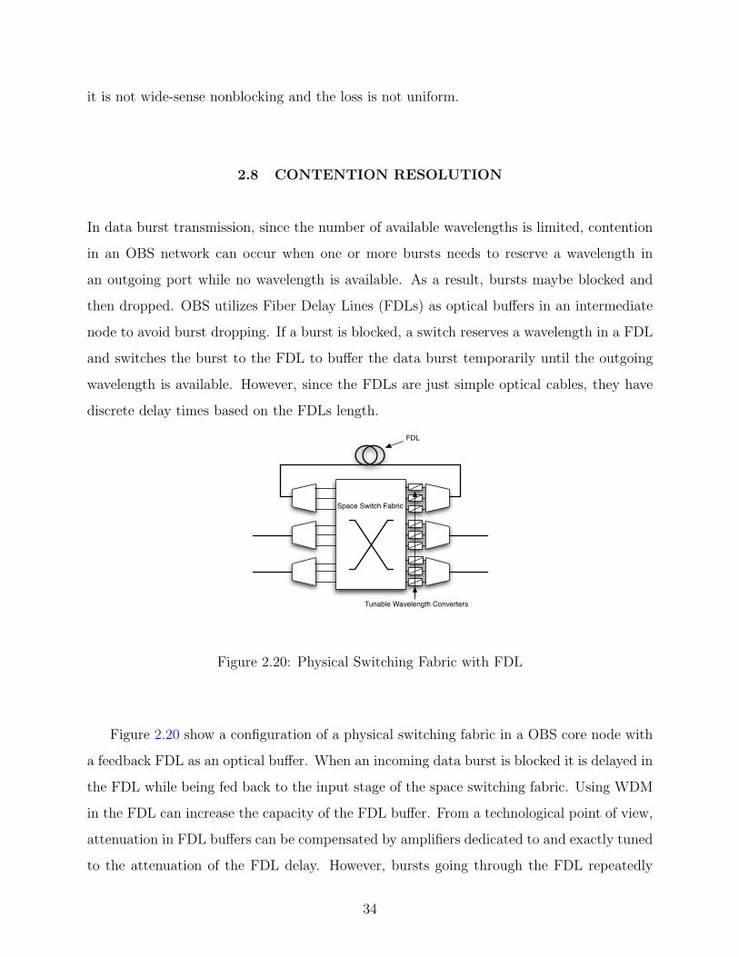
The Dilated Benes architecture [23] is a modified version of the Benes architecture in
order to solve Litium Niobate’s crosstalk problem. In Dilated Benes architecture shown
Figure 2.17: 8x8 Benes switch
32
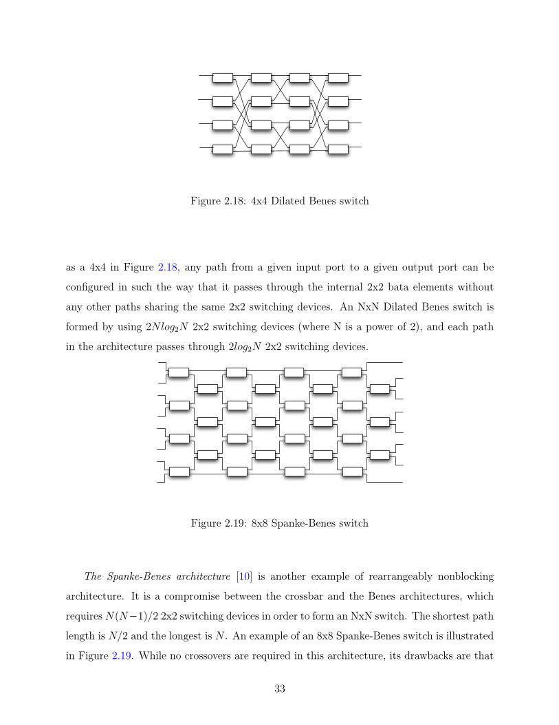
Figure 2.18: 4x4 Dilated Benes switch
as a 4x4 in Figure 2.18, any path from a given input port to a given output port can be
configured in such the way that it passes through the internal 2x2 bata elements without
any other paths sharing the same 2x2 switching devices. An NxN Dilated Benes switch is
formed by using 2Nlog2N 2x2 switching devices (where N is a power of 2), and each path
in the architecture passes through 2log2N 2x2 switching devices.
Figure 2.19: 8x8 Spanke-Benes switch
The Spanke-Benes architecture [10] is another example of rearrangeably nonblocking
architecture. It is a compromise between the crossbar and the Benes architectures, which
requires N(N−1)/2 2x2 switching devices in order to form an NxN switch. The shortest path
length is N/2 and the longest is N . An example of an 8x8 Spanke-Benes switch is illustrated
in Figure 2.19. While no crossovers are required in this architecture, its drawbacks are that
33
it is not wide-sense nonblocking and the loss is not uniform.
2.8 CONTENTION RESOLUTION
In data burst transmission, since the number of available wavelengths is limited, contention
in an OBS network can occur when one or more bursts needs to reserve a wavelength in
an outgoing port while no wavelength is available. As a result, bursts maybe blocked and
then dropped. OBS utilizes Fiber Delay Lines (FDLs) as optical buffers in an intermediate
node to avoid burst dropping. If a burst is blocked, a switch reserves a wavelength in a FDL
and switches the burst to the FDL to buffer the data burst temporarily until the outgoing
wavelength is available. However, since the FDLs are just simple optical cables, they have
discrete delay times based on the FDLs length.
Space Switch Fabric
FDL
Tunable Wavelength Converters
Figure 2.20: Physical Switching Fabric with FDL
Figure 2.20 show a configuration of a physical switching fabric in a OBS core node with
a feedback FDL as an optical buffer. When an incoming data burst is blocked it is delayed in
the FDL while being fed back to the input stage of the space switching fabric. Using WDM
in the FDL can increase the capacity of the FDL buffer. From a technological point of view,
attenuation in FDL buffers can be compensated by amplifiers dedicated to and exactly tuned
to the attenuation of the FDL delay. However, bursts going through the FDL repeatedly
34
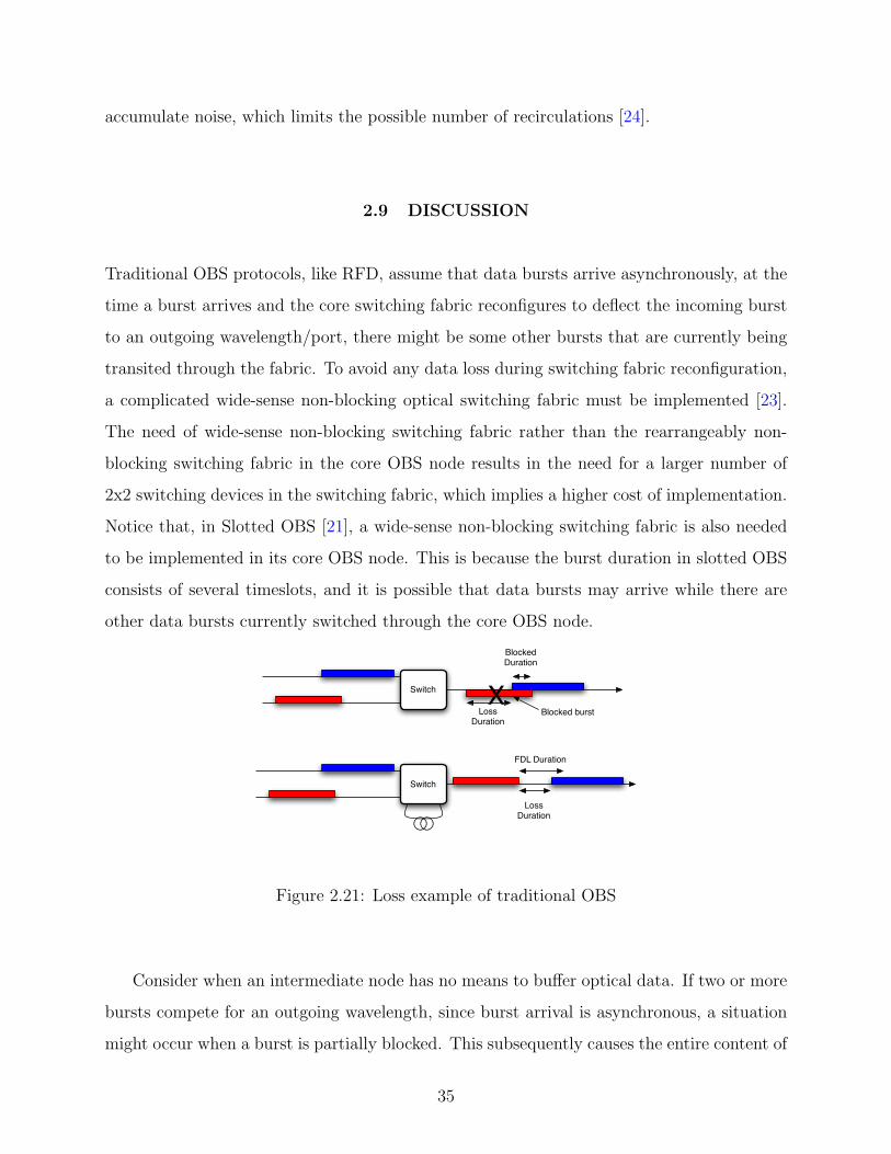
accumulate noise, which limits the possible number of recirculations [24].
2.9 DISCUSSION
Traditional OBS protocols, like RFD, assume that data bursts arrive asynchronously, at the
time a burst arrives and the core switching fabric reconfigures to deflect the incoming burst
to an outgoing wavelength/port, there might be some other bursts that are currently being
transited through the fabric. To avoid any data loss during switching fabric reconfiguration,
a complicated wide-sense non-blocking optical switching fabric must be implemented [23].
The need of wide-sense non-blocking switching fabric rather than the rearrangeably non-
blocking switching fabric in the core OBS node results in the need for a larger number of
2x2 switching devices in the switching fabric, which implies a higher cost of implementation.
Notice that, in Slotted OBS [21], a wide-sense non-blocking switching fabric is also needed
to be implemented in its core OBS node. This is because the burst duration in slotted OBS
consists of several timeslots, and it is possible that data bursts may arrive while there are
other data bursts currently switched through the core OBS node.
Switch
Blocked Duration
Loss Duration
XBlocked burst
Switch
FDL Duration
Loss Duration
Figure 2.21: Loss example of traditional OBS
Consider when an intermediate node has no means to buffer optical data. If two or more
bursts compete for an outgoing wavelength, since burst arrival is asynchronous, a situation
might occur when a burst is partially blocked. This subsequently causes the entire content of
35
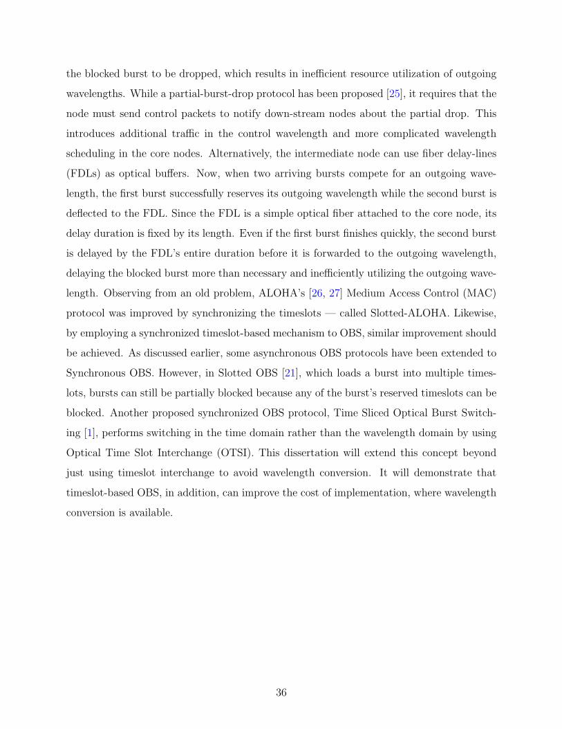
the blocked burst to be dropped, which results in inefficient resource utilization of outgoing
wavelengths. While a partial-burst-drop protocol has been proposed [25], it requires that the
node must send control packets to notify down-stream nodes about the partial drop. This
introduces additional traffic in the control wavelength and more complicated wavelength
scheduling in the core nodes. Alternatively, the intermediate node can use fiber delay-lines
(FDLs) as optical buffers. Now, when two arriving bursts compete for an outgoing wave-
length, the first burst successfully reserves its outgoing wavelength while the second burst is
deflected to the FDL. Since the FDL is a simple optical fiber attached to the core node, its
delay duration is fixed by its length. Even if the first burst finishes quickly, the second burst
is delayed by the FDL’s entire duration before it is forwarded to the outgoing wavelength,
delaying the blocked burst more than necessary and inefficiently utilizing the outgoing wave-
length. Observing from an old problem, ALOHA’s [26, 27] Medium Access Control (MAC)
protocol was improved by synchronizing the timeslots — called Slotted-ALOHA. Likewise,
by employing a synchronized timeslot-based mechanism to OBS, similar improvement should
be achieved. As discussed earlier, some asynchronous OBS protocols have been extended to
Synchronous OBS. However, in Slotted OBS [21], which loads a burst into multiple times-
lots, bursts can still be partially blocked because any of the burst’s reserved timeslots can be
blocked. Another proposed synchronized OBS protocol, Time Sliced Optical Burst Switch-
ing [1], performs switching in the time domain rather than the wavelength domain by using
Optical Time Slot Interchange (OTSI). This dissertation will extend this concept beyond
just using timeslot interchange to avoid wavelength conversion. It will demonstrate that
timeslot-based OBS, in addition, can improve the cost of implementation, where wavelength
conversion is available.
36
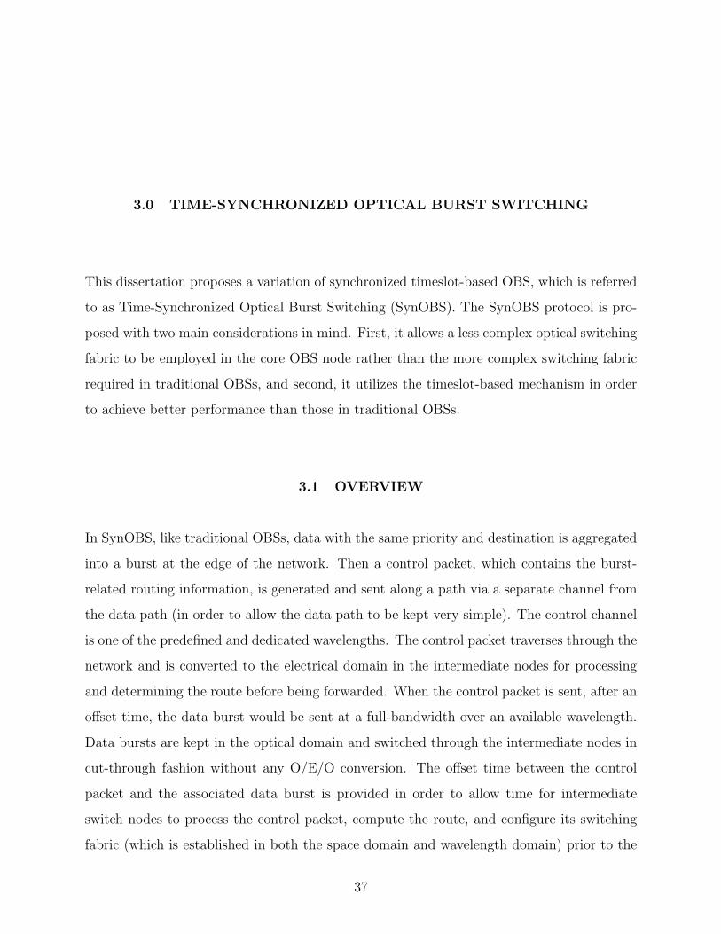
3.0 TIME-SYNCHRONIZED OPTICAL BURST SWITCHING
This dissertation proposes a variation of synchronized timeslot-based OBS, which is referred
to as Time-Synchronized Optical Burst Switching (SynOBS). The SynOBS protocol is pro-
posed with two main considerations in mind. First, it allows a less complex optical switching
fabric to be employed in the core OBS node rather than the more complex switching fabric
required in traditional OBSs, and second, it utilizes the timeslot-based mechanism in order
to achieve better performance than those in traditional OBSs.
3.1 OVERVIEW
In SynOBS, like traditional OBSs, data with the same priority and destination is aggregated
into a burst at the edge of the network. Then a control packet, which contains the burst-
related routing information, is generated and sent along a path via a separate channel from
the data path (in order to allow the data path to be kept very simple). The control channel
is one of the predefined and dedicated wavelengths. The control packet traverses through the
network and is converted to the electrical domain in the intermediate nodes for processing
and determining the route before being forwarded. When the control packet is sent, after an
offset time, the data burst would be sent at a full-bandwidth over an available wavelength.
Data bursts are kept in the optical domain and switched through the intermediate nodes in
cut-through fashion without any O/E/O conversion. The offset time between the control
packet and the associated data burst is provided in order to allow time for intermediate
switch nodes to process the control packet, compute the route, and configure its switching
fabric (which is established in both the space domain and wavelength domain) prior to the
37
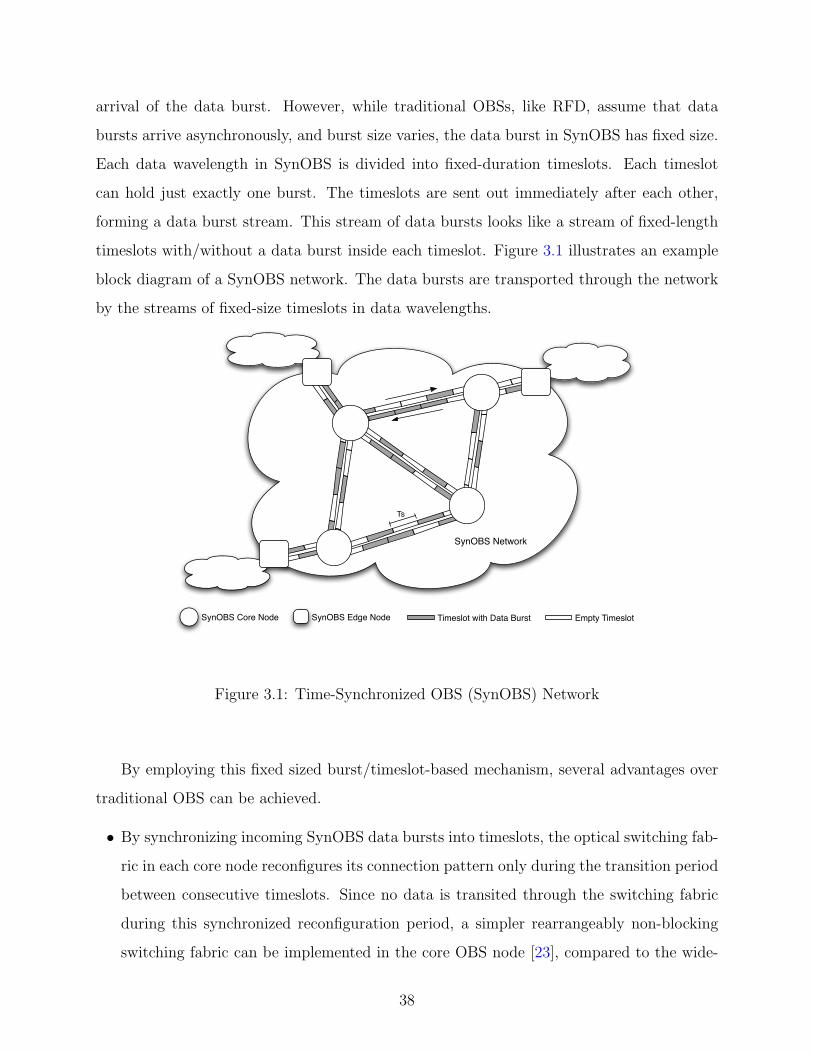
arrival of the data burst. However, while traditional OBSs, like RFD, assume that data
bursts arrive asynchronously, and burst size varies, the data burst in SynOBS has fixed size.
Each data wavelength in SynOBS is divided into fixed-duration timeslots. Each timeslot
can hold just exactly one burst. The timeslots are sent out immediately after each other,
forming a data burst stream. This stream of data bursts looks like a stream of fixed-length
timeslots with/without a data burst inside each timeslot. Figure 3.1 illustrates an example
block diagram of a SynOBS network. The data bursts are transported through the network
by the streams of fixed-size timeslots in data wavelengths.
Ts
SynOBS Network
SynOBS Core Node SynOBS Edge Node Timeslot with Data Burst Empty Timeslot
Figure 3.1: Time-Synchronized OBS (SynOBS) Network
By employing this fixed sized burst/timeslot-based mechanism, several advantages over
traditional OBS can be achieved.
• By synchronizing incoming SynOBS data bursts into timeslots, the optical switching fab-
ric in each core node reconfigures its connection pattern only during the transition period
between consecutive timeslots. Since no data is transited through the switching fabric
during this synchronized reconfiguration period, a simpler rearrangeably non-blocking
switching fabric can be implemented in the core OBS node [23], compared to the wide-
38
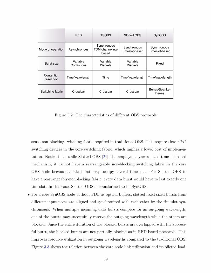
RFD TSOBS Slotted OBS SynOBS
Mode of operation Asynchronous
Synchronous
TDM channeling-
based
Synchronous
Timeslot-based
Synchronous
Timeslot-based
Burst sizeVariable
Continuous
Variable
Discrete
Variable
DiscreteFixed
Contention
resolutionTime/wavelength Time Time/wavelength Time/wavelength
Switching fabric Crossbar Crossbar CrossbarBenes/Spanke-
Benes
Figure 3.2: The characteristics of different OBS protocols
sense non-blocking switching fabric required in traditional OBS. This requires fewer 2x2
switching devices in the core switching fabric, which implies a lower cost of implemen-
tation. Notice that, while Slotted OBS [21] also employs a synchronized timeslot-based
mechanism, it cannot have a rearrangeably non-blocking switching fabric in the core
OBS node because a data burst may occupy several timeslots. For Slotted OBS to
have a rearrangeably-nonblocking fabric, every data burst would have to last exactly one
timeslot. In this case, Slotted OBS is transformed to be SynOBS.
• For a core SynOBS node without FDL as optical buffers, slotted fixed-sized bursts from
different input ports are aligned and synchronized with each other by the timeslot syn-
chronizers. When multiple incoming data bursts compete for an outgoing wavelength,
one of the bursts may successfully reserve the outgoing wavelength while the others are
blocked. Since the entire duration of the blocked bursts are overlapped with the success-
ful burst, the blocked bursts are not partially blocked as in RFD-based protocols. This
improves resource utilization in outgoing wavelengths compared to the traditional OBS.
Figure 3.3 shows the relation between the core node link utilization and its offered load,
39
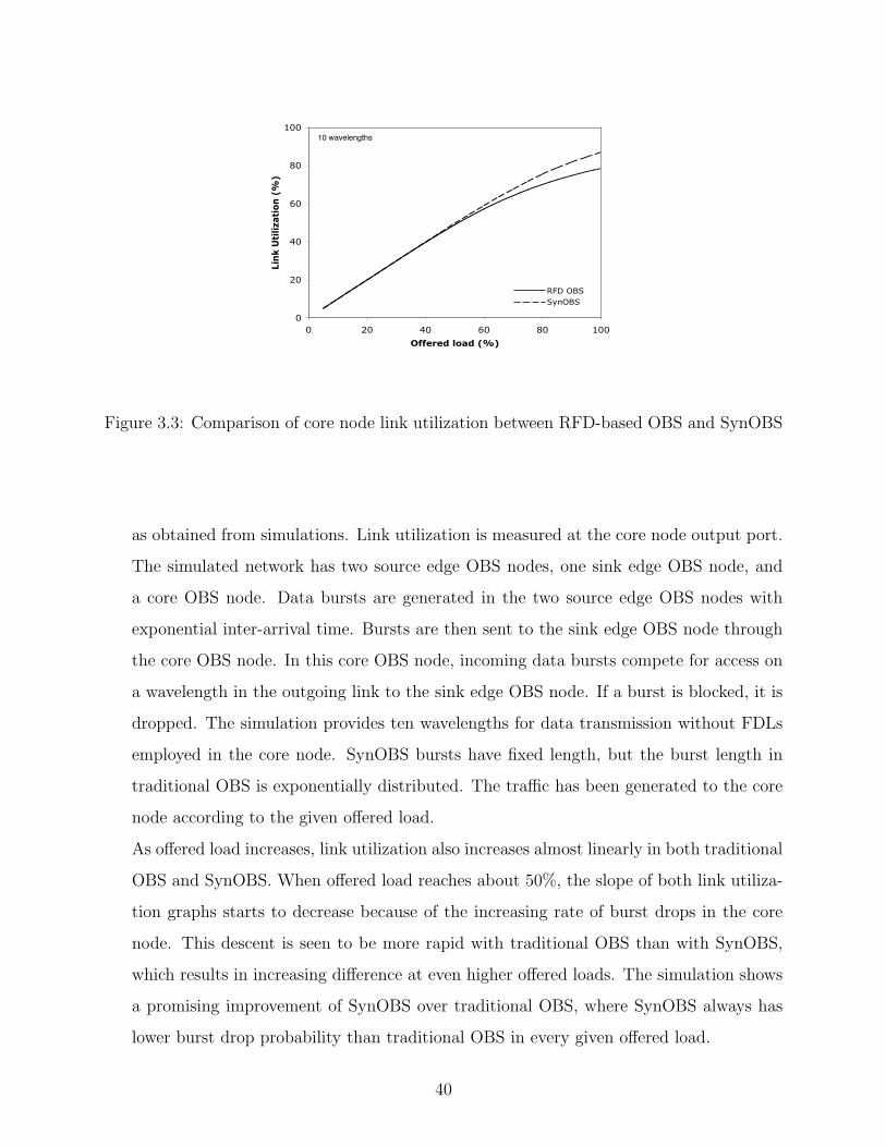
0
20
40
60
80
100
0 20 40 60 80 100
Offered load (%)
Lin
k U
tili
zati
on
(%
)
RFD OBSSynOBS
10 wavelengths
Figure 3.3: Comparison of core node link utilization between RFD-based OBS and SynOBS
as obtained from simulations. Link utilization is measured at the core node output port.
The simulated network has two source edge OBS nodes, one sink edge OBS node, and
a core OBS node. Data bursts are generated in the two source edge OBS nodes with
exponential inter-arrival time. Bursts are then sent to the sink edge OBS node through
the core OBS node. In this core OBS node, incoming data bursts compete for access on
a wavelength in the outgoing link to the sink edge OBS node. If a burst is blocked, it is
dropped. The simulation provides ten wavelengths for data transmission without FDLs
employed in the core node. SynOBS bursts have fixed length, but the burst length in
traditional OBS is exponentially distributed. The traffic has been generated to the core
node according to the given offered load.
As offered load increases, link utilization also increases almost linearly in both traditional
OBS and SynOBS. When offered load reaches about 50%, the slope of both link utiliza-
tion graphs starts to decrease because of the increasing rate of burst drops in the core
node. This descent is seen to be more rapid with traditional OBS than with SynOBS,
which results in increasing difference at even higher offered loads. The simulation shows
a promising improvement of SynOBS over traditional OBS, where SynOBS always has
lower burst drop probability than traditional OBS in every given offered load.
40
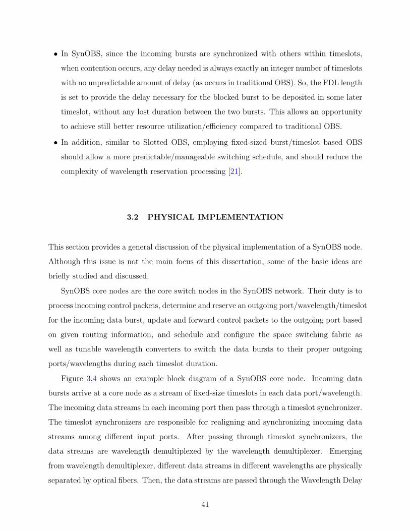
• In SynOBS, since the incoming bursts are synchronized with others within timeslots,
when contention occurs, any delay needed is always exactly an integer number of timeslots
with no unpredictable amount of delay (as occurs in traditional OBS). So, the FDL length
is set to provide the delay necessary for the blocked burst to be deposited in some later
timeslot, without any lost duration between the two bursts. This allows an opportunity
to achieve still better resource utilization/efficiency compared to traditional OBS.
• In addition, similar to Slotted OBS, employing fixed-sized burst/timeslot based OBS
should allow a more predictable/manageable switching schedule, and should reduce the
complexity of wavelength reservation processing [21].
3.2 PHYSICAL IMPLEMENTATION
This section provides a general discussion of the physical implementation of a SynOBS node.
Although this issue is not the main focus of this dissertation, some of the basic ideas are
briefly studied and discussed.
SynOBS core nodes are the core switch nodes in the SynOBS network. Their duty is to
process incoming control packets, determine and reserve an outgoing port/wavelength/timeslot
for the incoming data burst, update and forward control packets to the outgoing port based
on given routing information, and schedule and configure the space switching fabric as
well as tunable wavelength converters to switch the data bursts to their proper outgoing
ports/wavelengths during each timeslot duration.
Figure 3.4 shows an example block diagram of a SynOBS core node. Incoming data
bursts arrive at a core node as a stream of fixed-size timeslots in each data port/wavelength.
The incoming data streams in each incoming port then pass through a timeslot synchronizer.
The timeslot synchronizers are responsible for realigning and synchronizing incoming data
streams among different input ports. After passing through timeslot synchronizers, the
data streams are wavelength demultiplexed by the wavelength demultiplexer. Emerging
from wavelength demultiplexer, different data streams in different wavelengths are physically
separated by optical fibers. Then, the data streams are passed through the Wavelength Delay
41
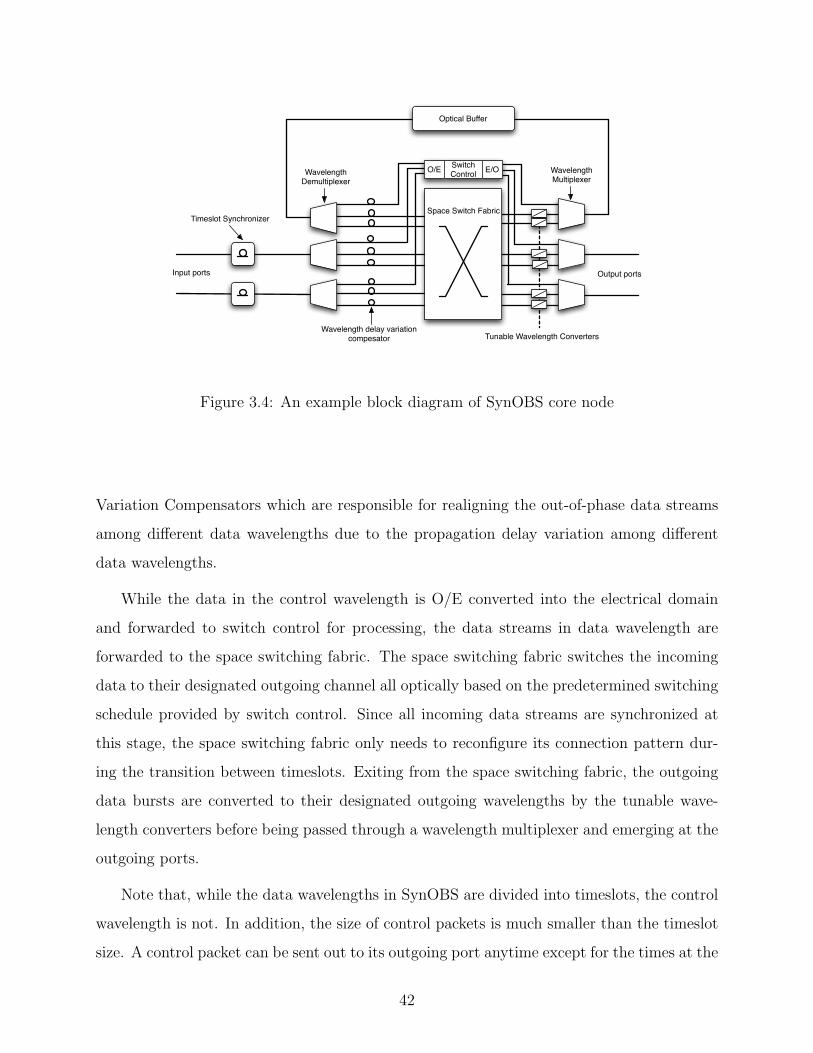
Timeslot Synchronizer
Switch Control E/O
Space Switch Fabric
O/E
Input ports Output ports
Optical Buffer
Tunable Wavelength Converters
Wavelength Multiplexer
Wavelength Demultiplexer
Wavelength delay variationcompesator
Figure 3.4: An example block diagram of SynOBS core node
Variation Compensators which are responsible for realigning the out-of-phase data streams
among different data wavelengths due to the propagation delay variation among different
data wavelengths.
While the data in the control wavelength is O/E converted into the electrical domain
and forwarded to switch control for processing, the data streams in data wavelength are
forwarded to the space switching fabric. The space switching fabric switches the incoming
data to their designated outgoing channel all optically based on the predetermined switching
schedule provided by switch control. Since all incoming data streams are synchronized at
this stage, the space switching fabric only needs to reconfigure its connection pattern dur-
ing the transition between timeslots. Exiting from the space switching fabric, the outgoing
data bursts are converted to their designated outgoing wavelengths by the tunable wave-
length converters before being passed through a wavelength multiplexer and emerging at the
outgoing ports.
Note that, while the data wavelengths in SynOBS are divided into timeslots, the control
wavelength is not. In addition, the size of control packets is much smaller than the timeslot
size. A control packet can be sent out to its outgoing port anytime except for the times at the
42

start of each timeslot. This time is reserved for the synchronization signal (shown as spikes
on the control channels in Figure 3.5) which is used by SynOBS nodes for synchronization
purposes.
3.2.1 Synchronization
In timeslot-based OBS, a mechanism to realign and synchronize incoming data streams from
different incoming ports and wavelengths is mandatory. For SynOBS, timeslot synchronizers
and wavelength delay variation compensators are used to synchronize these incoming data
streams. The timeslot synchronizers are responsible for realigning the different incoming
data streams from different incoming ports that arrive out of phase compared to each other.
Additionally, out-of-phase data streams among different data wavelengths on the same in-
coming port (caused by variation of each stream’s speed at different wavelengths) can be
realigned by wavelength delay variation compensators.
Control Channel
Space SwitchingFabric
Timeslot Synchronizer
Wavelength Demultiplexer
Wavelength delay variationcompesator
Figure 3.5: An example block diagram of SynOBS timing
Figure 3.5 illustrates a timing example of the incoming data streams arriving at a SynOBS
core node. When the data streams arrive at a node (the left most part of the Figure),they
are out of phase across different input ports and across different wavelengths on the same
incoming port. Based on the synchronization signal given in the control channel (synchro-
nization pluses), the core node adjusts the delay duration of the timeslot synchronizers to
delay and synchronize the incoming data streams from different incoming ports with its in-
43
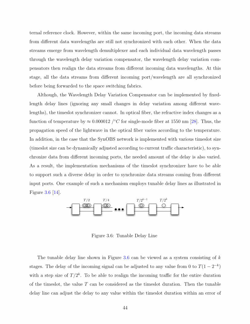
ternal reference clock. However, within the same incoming port, the incoming data streams
from different data wavelengths are still not synchronized with each other. When the data
streams emerge from wavelength demultiplexer and each individual data wavelength passes
through the wavelength delay variation compensator, the wavelength delay variation com-
pensators then realign the data streams from different incoming data wavelengths. At this
stage, all the data streams from different incoming port/wavelength are all synchronized
before being forwarded to the space switching fabrics.
Although, the Wavelength Delay Variation Compensator can be implemented by fixed-
length delay lines (ignoring any small changes in delay variation among different wave-
lengths), the timeslot synchronizer cannot. In optical fiber, the refractive index changes as a
function of temperature by ≈ 0.000012 /◦C for single-mode fiber at 1550 nm [28]. Thus, the
propagation speed of the lightwave in the optical fiber varies according to the temperature.
In addition, in the case that the SynOBS network is implemented with various timeslot size
(timeslot size can be dynamically adjusted according to current traffic characteristic), to syn-
chronize data from different incoming ports, the needed amount of the delay is also varied.
As a result, the implementation mechanisms of the timeslot synchronizer have to be able
to support such a diverse delay in order to synchronize data streams coming from different
input ports. One example of such a mechanism employs tunable delay lines as illustrated in
Figure 3.6 [14].
T/2 T/4 T/2k!1 T/2
k
Figure 3.6: Tunable Delay Line
The tunable delay line shown in Figure 3.6 can be viewed as a system consisting of k
stages. The delay of the incoming signal can be adjusted to any value from 0 to T (1− 2−k)
with a step size of T/2k. To be able to realign the incoming traffic for the entire duration
of the timeslot, the value T can be considered as the timeslot duration. Then the tunable
delay line can adjust the delay to any value within the timeslot duration within an error of
44
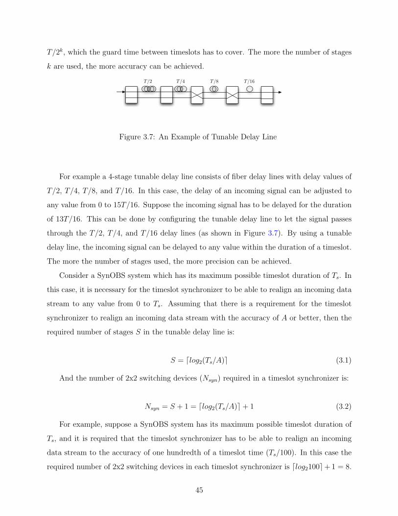
T/2k, which the guard time between timeslots has to cover. The more the number of stages
k are used, the more accuracy can be achieved.
T/8T/4T/2 T/16
Figure 3.7: An Example of Tunable Delay Line
For example a 4-stage tunable delay line consists of fiber delay lines with delay values of
T/2, T/4, T/8, and T/16. In this case, the delay of an incoming signal can be adjusted to
any value from 0 to 15T/16. Suppose the incoming signal has to be delayed for the duration
of 13T/16. This can be done by configuring the tunable delay line to let the signal passes
through the T/2, T/4, and T/16 delay lines (as shown in Figure 3.7). By using a tunable
delay line, the incoming signal can be delayed to any value within the duration of a timeslot.
The more the number of stages used, the more precision can be achieved.
Consider a SynOBS system which has its maximum possible timeslot duration of Ts. In
this case, it is necessary for the timeslot synchronizer to be able to realign an incoming data
stream to any value from 0 to Ts. Assuming that there is a requirement for the timeslot
synchronizer to realign an incoming data stream with the accuracy of A or better, then the
required number of stages S in the tunable delay line is:
S = dlog2(Ts/A)e (3.1)
And the number of 2x2 switching devices (Nsyn) required in a timeslot synchronizer is:
Nsyn = S + 1 = dlog2(Ts/A)e+ 1 (3.2)
For example, suppose a SynOBS system has its maximum possible timeslot duration of
Ts, and it is required that the timeslot synchronizer has to be able to realign an incoming
data stream to the accuracy of one hundredth of a timeslot time (Ts/100). In this case the
required number of 2x2 switching devices in each timeslot synchronizer is dlog2100e+ 1 = 8.
45
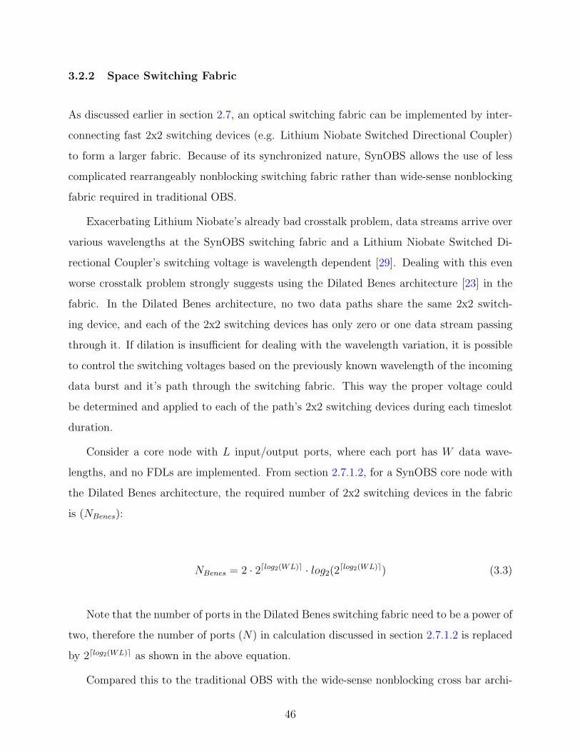
3.2.2 Space Switching Fabric
As discussed earlier in section 2.7, an optical switching fabric can be implemented by inter-
connecting fast 2x2 switching devices (e.g. Lithium Niobate Switched Directional Coupler)
to form a larger fabric. Because of its synchronized nature, SynOBS allows the use of less
complicated rearrangeably nonblocking switching fabric rather than wide-sense nonblocking
fabric required in traditional OBS.
Exacerbating Lithium Niobate’s already bad crosstalk problem, data streams arrive over
various wavelengths at the SynOBS switching fabric and a Lithium Niobate Switched Di-
rectional Coupler’s switching voltage is wavelength dependent [29]. Dealing with this even
worse crosstalk problem strongly suggests using the Dilated Benes architecture [23] in the
fabric. In the Dilated Benes architecture, no two data paths share the same 2x2 switch-
ing device, and each of the 2x2 switching devices has only zero or one data stream passing
through it. If dilation is insufficient for dealing with the wavelength variation, it is possible
to control the switching voltages based on the previously known wavelength of the incoming
data burst and it’s path through the switching fabric. This way the proper voltage could
be determined and applied to each of the path’s 2x2 switching devices during each timeslot
duration.
Consider a core node with L input/output ports, where each port has W data wave-
lengths, and no FDLs are implemented. From section 2.7.1.2, for a SynOBS core node with
the Dilated Benes architecture, the required number of 2x2 switching devices in the fabric
is (NBenes):
NBenes = 2 · 2dlog2(WL)e · log2(2dlog2(WL)e) (3.3)
Note that the number of ports in the Dilated Benes switching fabric need to be a power of
two, therefore the number of ports (N) in calculation discussed in section 2.7.1.2 is replaced
by 2dlog2(WL)e as shown in the above equation.
Compared this to the traditional OBS with the wide-sense nonblocking cross bar archi-
46
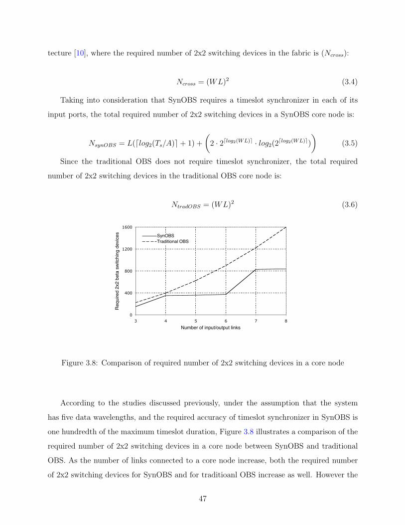
tecture [10], where the required number of 2x2 switching devices in the fabric is (Ncross):
Ncross = (WL)2 (3.4)
Taking into consideration that SynOBS requires a timeslot synchronizer in each of its
input ports, the total required number of 2x2 switching devices in a SynOBS core node is:
NsynOBS = L(dlog2(Ts/A)e+ 1) +
(2 · 2dlog2(WL)e · log2(2
dlog2(WL)e)
)(3.5)
Since the traditional OBS does not require timeslot synchronizer, the total required
number of 2x2 switching devices in the traditional OBS core node is:
NtradOBS = (WL)2 (3.6)
0
400
800
1200
1600
3 4 5 6 7 8
Number of input/output links
Requ
ired
2x2
beta
swi
tchi
ng d
evice
s SynOBSTraditional OBS
Figure 3.8: Comparison of required number of 2x2 switching devices in a core node
According to the studies discussed previously, under the assumption that the system
has five data wavelengths, and the required accuracy of timeslot synchronizer in SynOBS is
one hundredth of the maximum timeslot duration, Figure 3.8 illustrates a comparison of the
required number of 2x2 switching devices in a core node between SynOBS and traditional
OBS. As the number of links connected to a core node increase, both the required number
of 2x2 switching devices for SynOBS and for traditioanl OBS increase as well. However the
47
required numbers in traditional OBS is almost always greater than those in SynOBS. This
implies that implementation of a SynOBS core node is cheaper and more scalable than a
traditional OBS core node.
3.2.3 Tunable Wavelength Converter
The tunable wavelength converter is responsible for converting the wavelength of the in-
coming data burst to its designated outgoing wavelength before the burst is sent out to
the outgoing port. As discussed earlier in section 2.7, the tunable wavelength converter for
all-optical network has received increasing attention and become an active area of research
recently [10, 23]. The three basic mechanisms for wavelength conversion include Optoelec-
tronic Conversion, Optical Gating Wavelength Conversion, and Wave-Mixing Wavelength
Conversion. Although these technologies are still far from being mature, this research as-
sumes that the provided tunable wavelength converters have full capability of wavelength
conversion — which means, they can convert any given input data wavelength to any output
data wavelength. One simple example of such a full capability of wavelength conversion is
the pair of a photodetector and a tunable laser.
In a SynOBS core node, the number of tunable wavelength converters (Nwlc) is
Nwlc = (L+ F ) ·W (3.7)
where, L is the number of outgoing ports, F is the number of optical buffers in the node,
and W is the number of available data wavelengths. For example, in Figure 3.4, the SynOBS
core node has two input/output port pairs, one optical buffer, and two data wavelengths;
thus, the number of tunable wavelength converters in this node is six.
In order to reduce the number of required tunable wavelength converters in a SynOBS
node, several shared tunable wavelength converters mechanisms have been proposed [30, 31].
The basic idea of shared tunable wavelength converter mechanisms is basically to share a
pool of tunable wavelength converters among the outgoing wavelength/port pairs in the
node. However, this is not the focus of this dissertation, and for the sake of simplicity,
it is assumed that a dedicated tunable wavelength converter is provided for each outgoing
48
wavelength/port pair without sharing.
3.2.4 Wavelength Demultiplexer/Multiplexer
Wavelength demultiplexers in a SynOBS core node are responsible for demultiplexing and
separating the incoming WDM data streams. While the demultiplexed control wavelength
is forwarded to the O/E converter for control packet processing, the demultiplexed data
wavelengths are forwarded to the space switching fabric. On the other hand, wavelength
multiplexers are responsible for multiplexing the data streams on different outgoing wave-
lengths that are going out to the same output port. Wavelength demultiplexer/multiplexers
could be implemented from either grating demultiplexer or phase array wavelength demulti-
plexer [10]). The multiplexer could be a simple optical combiner if the power budget allows
that much loss.
In a SynOBS core node, the number of required wavelength demultiplexer/multiplexer
pairs is equal to the number of incoming/outgoing port pairs plus the number of optical
buffers (FDLs) in the node (Nmux = L + F ). For example, in Figure 3.4, the SynOBS
core node has two input/output port pairs and one optical buffer, therefore the number of
wavelength demultiplexer/multiplexer pairs required in this node is three (two plus one).
3.2.5 Switch Control
In the control wavelength, the data stream is converted into the electrical domain in order
to process the information in the control packets. After a control packet is converted to
electrical domain, it is then forwarded to switch control. The switch control acts as a
central brain of the SynOBS core node, where it reads the information given in the incoming
control packet, including: the incoming port, the incoming data wavelength, the incoming
timeslot, and the burst destination. The switch control then determines the outgoing port,
outgoing wavelength, and the outgoing timeslot for the incoming data burst based on the
information given from the control packet and the node’s current resource reservation. After
the outgoing port/wavelength/timeslot has been determined, the switch control reserves
this outgoing resource (as well as any optical buffer, that may be needed) and schedules the
49
space switching fabric and the tunable wavelength converter according to the reservation.
Besides, the switch control also updates the control packet associated with the data burst
and forwards it to the outgoing port in the control wavelength via E/O conversion.
The detailed resource reservation algorithm for the switch control will be further dis-
cussed in chapter 4.
3.2.6 Optical Buffer (FDL)
It is optional that a SynOBS core node be equipped with feedback Fiber Delay Lines (FDLs)
for buffering its data bursts. These feedback FDLs work as optical buffers in the core node
by forming a feedback delay-loop from the outgoing side back to the incoming side of the
switching fabric [24]. Whenever a data burst is buffered (delayed) in the core node, the
switching fabric switches the incoming data burst to an FDL. The burst is then buffered
in this FDL for the duration of the FDL’s length before it arrives at the FDL’s other end
on the incoming side of the switching fabric. Thereafter, this burst is either switched out
to its intended outgoing port or switched back to an FDL again if it needs to be buffered
for a longer period of time. As SynOBS operates upon a synchronized timeslot basis, the
delay needed will be the multiple number of timeslots and an FDL’s length can be set in
accordance with the delay duration of the multiple number of timeslots in order to delay the
blocked burst to other upcoming timeslots.
If the SynOBS network has fixed timeslot duration, the optical buffer can be made from
the fixed-length FDL which has its delay duration according to its configuration (the multiple
numbers of timeslots). However, if the network has variable timeslot duration, the optical
buffer must then be able to adjust itself to such variable timeslot duration configurable in
the network. Again, this can be done by utilizing the tunable delay line (discussed in section
3.2.1).
Consider a SynOBS system that uses tunable delay lines and has variable timeslot du-
ration between Tmin and Tmax. Recall that the possible number of timeslot size settings can
be any number in the order of 2k (where k is the number of stages in tunable delay line).
Let Tdiff be the difference between maximum timeslot size and minimum timeslot size
50
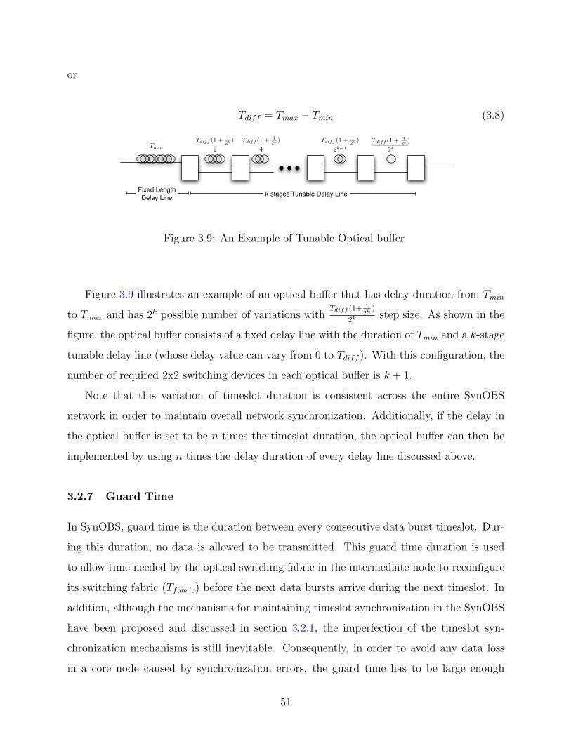
or
Tdiff = Tmax − Tmin (3.8)
k stages Tunable Delay LineFixed LengthDelay Line
Tdiff (1 + 1
2k )
4
Tdiff (1 + 1
2k )
2
Tdiff (1 + 1
2k )
2k!1
Tdiff (1 + 1
2k )
2kTmin
Figure 3.9: An Example of Tunable Optical buffer
Figure 3.9 illustrates an example of an optical buffer that has delay duration from Tmin
to Tmax and has 2k possible number of variations withTdiff (1+ 1
2k)
2kstep size. As shown in the
figure, the optical buffer consists of a fixed delay line with the duration of Tmin and a k-stage
tunable delay line (whose delay value can vary from 0 to Tdiff ). With this configuration, the
number of required 2x2 switching devices in each optical buffer is k + 1.
Note that this variation of timeslot duration is consistent across the entire SynOBS
network in order to maintain overall network synchronization. Additionally, if the delay in
the optical buffer is set to be n times the timeslot duration, the optical buffer can then be
implemented by using n times the delay duration of every delay line discussed above.
3.2.7 Guard Time
In SynOBS, guard time is the duration between every consecutive data burst timeslot. Dur-
ing this duration, no data is allowed to be transmitted. This guard time duration is used
to allow time needed by the optical switching fabric in the intermediate node to reconfigure
its switching fabric (Tfabric) before the next data bursts arrive during the next timeslot. In
addition, although the mechanisms for maintaining timeslot synchronization in the SynOBS
have been proposed and discussed in section 3.2.1, the imperfection of the timeslot syn-
chronization mechanisms is still inevitable. Consequently, in order to avoid any data loss
in a core node caused by synchronization errors, the guard time has to be large enough
51
to cover these synchronization errors among different incoming data streams to the node.
These synchronization errors include the errors caused by the imperfection of the timeslot
synchronizers (ETS), the imperfection of wavelength delay variation compensators (EWC),
and other miscellaneous errors (Emisc) caused by other causes that have not been discussed
in this dissertation (e.g. temperature-dependent delay variation in optical fiber, core node
internal reference clock error, etc.).
Hence, in order to ensure that there will be no data loss resulting from the timeslot syn-
chronization errors during the switching fabric reconfiguration, the guard time duration (Tg)
must then be equal to or greater than the combination of the switching fabric reconfiguration
duration and all the timeslot synchronization errors, or
Tg ≥ (Tfabric + ETS + EWC + Emisc) (3.9)
For example, assume that the switching fabrics used in the core node are based on the
extremely fast Electro-optic Switches (Tfabric ≈ 1 nsec). Then, further assume that the
maximum timeslot size setting is 200 µsec (≈ 250 1000-byte IP packets in a 10 Gbps link)
and the timeslot synchronizers is set with the accuracy of one one-hundredth of the maximum
timeslot size. Under these assumptions, the errors caused by timeslot synchronizer (ETS) is
2 µsec.
The errors resulting from imperfect wavelength delay variation compensators can also
be explained by example. Assume the SynOBS WDM system uses the 1550 nm operating
region, with an estimated usable spectral band of 120 nm [32]. The refractive index varies
by wavelength around 0.0006 in single-mode fiber [28]. Assume the data bursts traverse the
fiber with a maximum distance about 5000 km (the approximate distance from the west cost
to the east coast of the United States). Based on these factors, without the delay variation
compensator, the maximum synchronization errors caused by wavelength delay variation is
approximately 10 µsec = 0.0006×5000×103
3×10⁸ .
Assuming the wavelength delay variation compensators can compensate about 60 percent
of the overall wavelength delay variation, then the synchronization errors caused by the
chromatic dispersion (EWC) reduce to approximately 4 µsec. Allowing another 1 µsec for
miscellaneous errors (Emisc), the guard time (Tg) of the synOBS system must be equal to or
52

greater than 7 µsec as a result.
53
4.0 PERFORMANCE ANALYSIS OF SYNOBS CORE NODE
This chapter discusses the performance analysis of a SynOBS core node with several FDL
reservation mechanisms. Discussion begins with the performance analysis of a SynOBS core
node with no FDLs provided, Then the chapter analyzes a SynOBS core node in which FDLs
are available as optical buffers including SynOBS with separated FDLs and SynOBS with
Shared FDLs [33]. The end of the chapter analyzes SynOBS with multiple length FDLs.
Note that the analysis provided in this chaper is based on the assumption that each data
burst has one hundred percent timeslot utilization (a data burst is fitted into a timeslot
without any void filling).
Similar to the performance analysis of the Asynchronous Transfer Mode (ATM), using a
discrete-time Markov model [34, 35, 36], SynOBS’s timeslot operation can also be analyzed
by utilizing the discrete-time Markov model. Contrary to ATM, the SynOBS system utilizes
Wavelength Division Multiplexing with several data channels (data wavelengths) available
for the outgoing data bursts (there is only one channel in ATM) in each of the outgoing
ports (and each of the FDLs) of the SynOBS core node.
4.1 SYNOBS CORE NODE WITHOUT FDL
First, a simple model of SynOBS, in which its core node doesn’t have FDLs as optical buffers,
is investigated. Consider an incoming data burst that arrives at a SynOBS core node that
has no FDLs. If all the outgoing wavelengths are already reserved, then this burst would have
to be dropped because there is no output wavelength available during the burst’s arriving
timeslot and there is no optical buffer where the blocked burst could be buffered and delayed
54
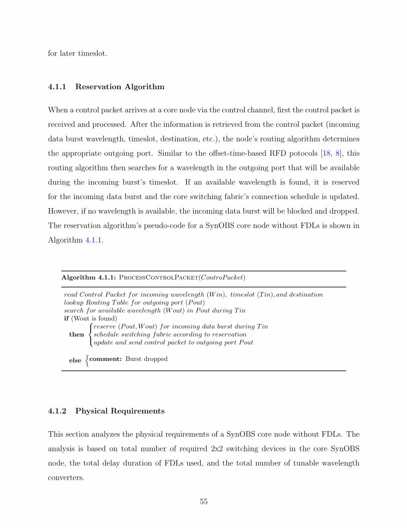
for later timeslot.
4.1.1 Reservation Algorithm
When a control packet arrives at a core node via the control channel, first the control packet is
received and processed. After the information is retrieved from the control packet (incoming
data burst wavelength, timeslot, destination, etc.), the node’s routing algorithm determines
the appropriate outgoing port. Similar to the offset-time-based RFD potocols [18, 8], this
routing algorithm then searches for a wavelength in the outgoing port that will be available
during the incoming burst’s timeslot. If an available wavelength is found, it is reserved
for the incoming data burst and the core switching fabric’s connection schedule is updated.
However, if no wavelength is available, the incoming data burst will be blocked and dropped.
The reservation algorithm’s pseudo-code for a SynOBS core node without FDLs is shown in
Algorithm 4.1.1.
Algorithm 4.1.1: ProcessControlPacket(ControPacket)
read Control Packet for incoming wavelength (Win), timeslot (Tin), and destinationlookup Routing Table for outgoing port (Pout)search for available wavelength (Wout) in Pout during T inif (Wout is found)
then
reserve (Pout, Wout) for incoming data burst during T inschedule switching fabric according to reservationupdate and send control packet to outgoing port Pout
else{comment: Burst dropped
4.1.2 Physical Requirements
This section analyzes the physical requirements of a SynOBS core node without FDLs. The
analysis is based on total number of required 2x2 switching devices in the core SynOBS
node, the total delay duration of FDLs used, and the total number of tunable wavelength
converters.
55
Consider a core node with L input/output ports, where each port has W data wave-
lengths, and no FDLs are implemented as optical buffers. Assuming the Dilated Benes
architecture is used in the space switching fabric, the required number of 2x2 switching
devices in the fabric is (NBenes):
NBenes = 2 · 2dlog2(WL)e · log2(2dlog2(WL)e) (4.1)
In addition, the SynOBS system with variable timeslot size requires a timeslot synchro-
nizer in each of the input ports, as described in Section 3.2.2. Then, the total required
number of 2x2 switching devices in a SynOBS core node is:
N2x2switches = L(dlog2(T/A)e+ 1) + 2 · 2dlog2(WL)e · log2(2dlog2(WL)e) (4.2)
Where, Ts is the maximum possible timeslot duration, and A is an accuracy requirement
of the timeslot synchronizers.
Since there are no FDLs used as optical buffers in the core node, FDLs are only required
in timeslot synchronizers and wavelength delay variation compensators. Assuming that
the amount of delay required in wavelength delay variation compensator is much smaller
than the maximum possible timeslot duration, the number of FDLs in the delay variation
compensators is negligible compared to the number in the timeslot synchronizers. Therefore,
the number of delay-duration FDLs’ required is Tmax · L.
With no optical buffers in the core node, the number of Tunable Wavelength Converters
(Nwlc) is
Nwlc = L ·W (4.3)
Where W is the number of available data wavelengths.
4.1.3 Blocking Analysis
In SynOBS without FDLs, since no FDLs are available for data bursts to be buffered in
the core nodes, blocking occurs whenever the number of data bursts scheduled to arrive at
an outgoing port at the start of the same timeslot is greater than the number of outgoing
56
wavelengths at this outgoing port. Assume the number of data bursts arriving at an outgoing
port during a given timeslot is Poisson distributed [37] with mean λ. Then, the probability
that n bursts arrive at the start of a timeslot is:
In =λne−λ
n!(4.4)
The maximum number of data bursts that could be successfully sent to an outgoing port
during some timeslot equals the number of outgoing wavelengths. Therefore, with W data
wavelengths available per outgoing link and n arrivals at the timeslot, the number of blocked
bursts (nblock|n) is:
nblock|n =
n−W if n > W
0 if n ≤ W(4.5)
Then, the expected number of blocked bursts (E[nblock]) during a timeslot is obtained
by:
E[nblock] =∞∑0
(In ∗ nblock|n)
=∞∑
n=W+1
[(n−W )λne−λ
n!] (4.6)
Since the average number of data bursts arriving at a timeslot is λ, the probability that
a data burst will be blocked (Pb) is calculated by:
Pb =E[nblock]
λ
=
∑∞n=W+1[(n−W )λ
ne−λ
n!]
λ(4.7)
Figure 4.1 and 4.2 show the performance of blocking probability in a SynOBS core node
without FDLs with respect to its offered load and the number of outgoing wavelengths. The
offered load is set according to the total outgoing throughput. For example, if the number
of outgoing wavelengths is W and offered load is O, then the average number of arrivals per
57
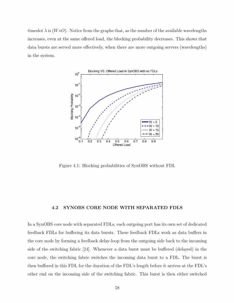
timeslot λ is (W ∗O). Notice from the graphs that, as the number of the available wavelengths
increases, even at the same offered load, the blocking probability decreases. This shows that
data bursts are served more effectively, when there are more outgoing servers (wavelengths)
in the system.
Figure 4.1: Blocking probabilities of SynOBS without FDL
4.2 SYNOBS CORE NODE WITH SEPARATED FDLS
In a SynOBS core node with separated FDLs, each outgoing port has its own set of dedicated
feedback FDLs for buffering its data bursts. These feedback FDLs work as data buffers in
the core node by forming a feedback delay-loop from the outgoing side back to the incoming
side of the switching fabric [24]. Whenever a data burst must be buffered (delayed) in the
core node, the switching fabric switches the incoming data burst to a FDL. The burst is
then buffered in this FDL for the duration of the FDL’s length before it arrives at the FDL’s
other end on the incoming side of the switching fabric. This burst is then either switched
58
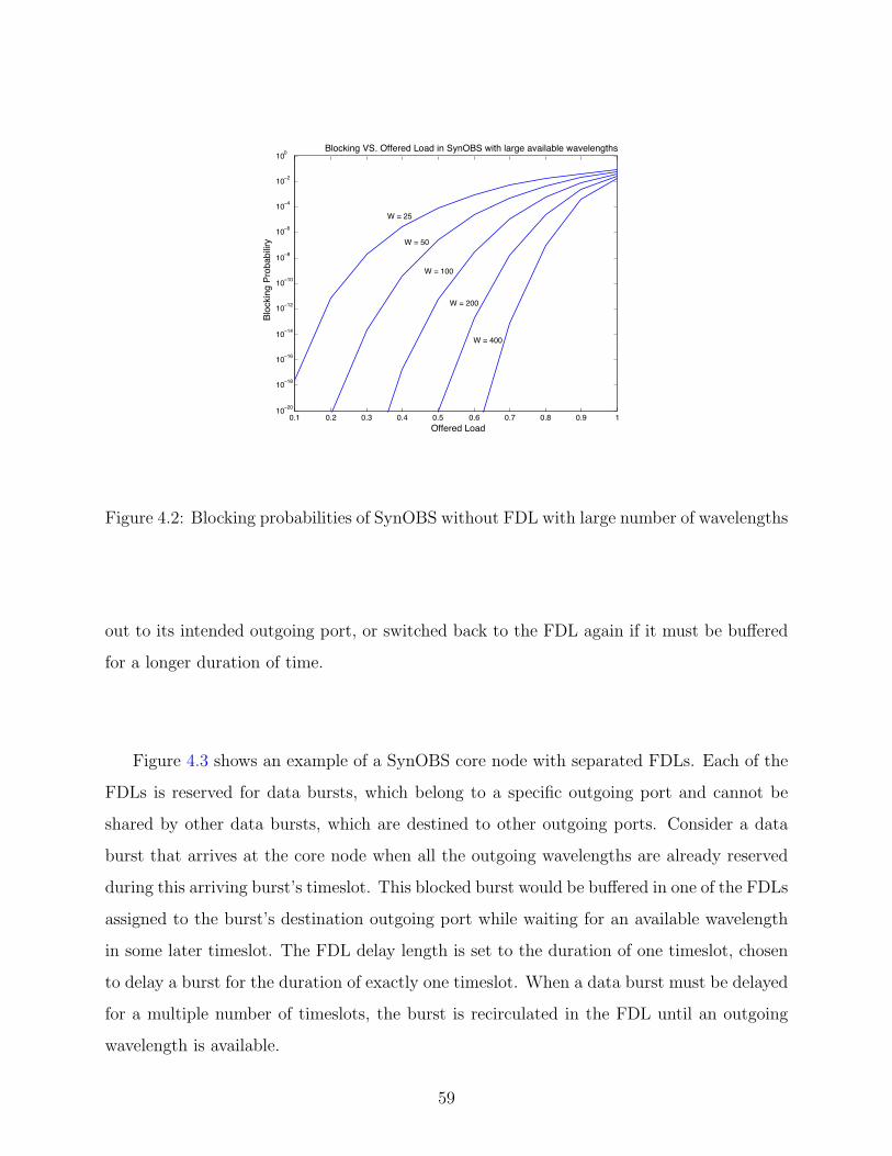
0.1 0.2 0.3 0.4 0.5 0.6 0.7 0.8 0.9 110
!20
10!18
10!16
10!14
10!12
10!10
10!8
10!6
10!4
10!2
100
Blocking VS. Offered Load in SynOBS with large available wavelengths
Blo
ckin
g P
rob
ab
iliry
Offered Load
W = 25
W = 50
W = 100
W = 200
W = 400
Figure 4.2: Blocking probabilities of SynOBS without FDL with large number of wavelengths
out to its intended outgoing port, or switched back to the FDL again if it must be buffered
for a longer duration of time.
Figure 4.3 shows an example of a SynOBS core node with separated FDLs. Each of the
FDLs is reserved for data bursts, which belong to a specific outgoing port and cannot be
shared by other data bursts, which are destined to other outgoing ports. Consider a data
burst that arrives at the core node when all the outgoing wavelengths are already reserved
during this arriving burst’s timeslot. This blocked burst would be buffered in one of the FDLs
assigned to the burst’s destination outgoing port while waiting for an available wavelength
in some later timeslot. The FDL delay length is set to the duration of one timeslot, chosen
to delay a burst for the duration of exactly one timeslot. When a data burst must be delayed
for a multiple number of timeslots, the burst is recirculated in the FDL until an outgoing
wavelength is available.
59
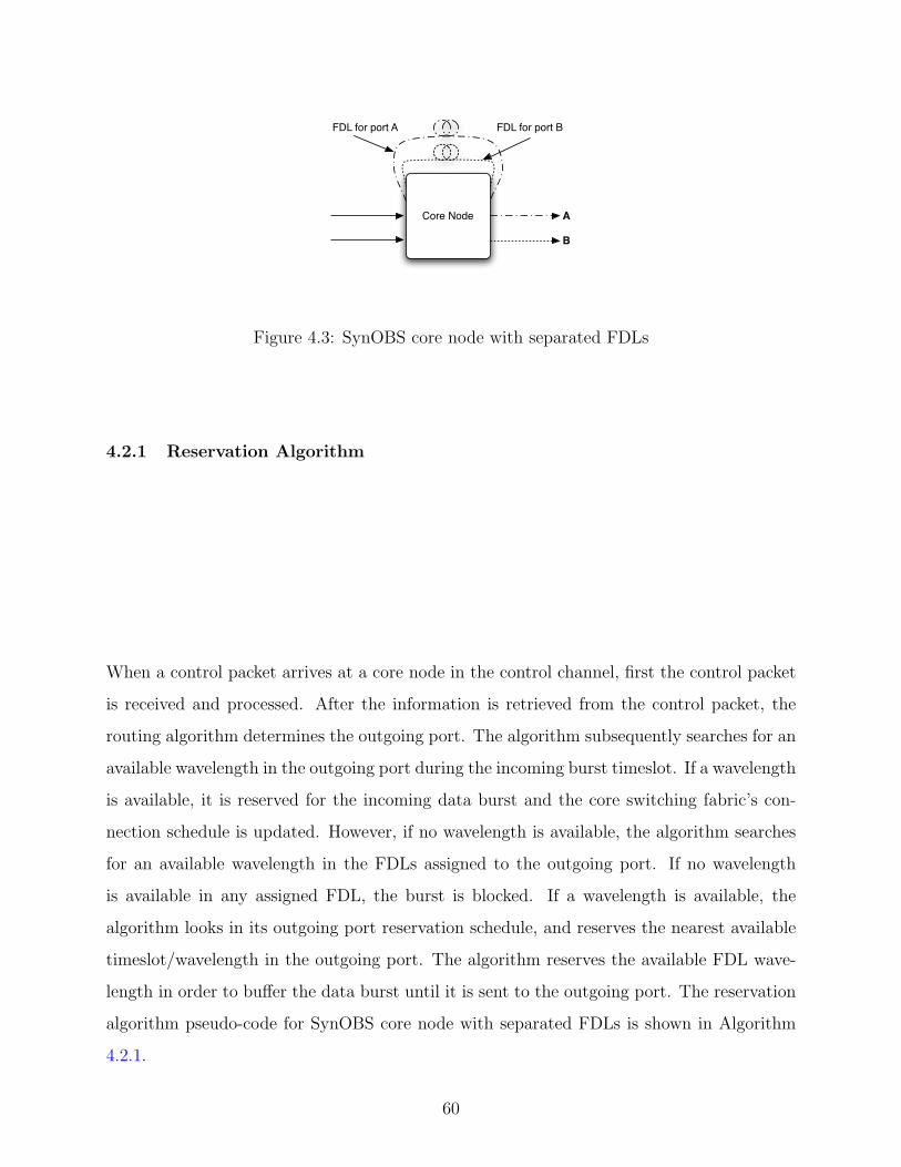
Core Node
FDL for port B
A
B
FDL for port A
Figure 4.3: SynOBS core node with separated FDLs
4.2.1 Reservation Algorithm
When a control packet arrives at a core node in the control channel, first the control packet
is received and processed. After the information is retrieved from the control packet, the
routing algorithm determines the outgoing port. The algorithm subsequently searches for an
available wavelength in the outgoing port during the incoming burst timeslot. If a wavelength
is available, it is reserved for the incoming data burst and the core switching fabric’s con-
nection schedule is updated. However, if no wavelength is available, the algorithm searches
for an available wavelength in the FDLs assigned to the outgoing port. If no wavelength
is available in any assigned FDL, the burst is blocked. If a wavelength is available, the
algorithm looks in its outgoing port reservation schedule, and reserves the nearest available
timeslot/wavelength in the outgoing port. The algorithm reserves the available FDL wave-
length in order to buffer the data burst until it is sent to the outgoing port. The reservation
algorithm pseudo-code for SynOBS core node with separated FDLs is shown in Algorithm
4.2.1.
60
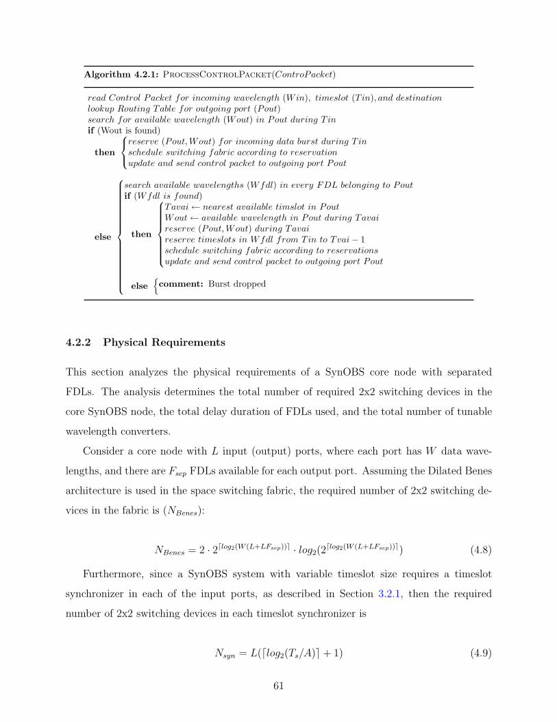
Algorithm 4.2.1: ProcessControlPacket(ControPacket)
read Control Packet for incoming wavelength (Win), timeslot (Tin), and destinationlookup Routing Table for outgoing port (Pout)search for available wavelength (Wout) in Pout during T inif (Wout is found)
then
reserve (Pout, Wout) for incoming data burst during T inschedule switching fabric according to reservationupdate and send control packet to outgoing port Pout
else
search available wavelengths (Wfdl) in every FDL belonging to Poutif (Wfdl is found)
then
Tavai← nearest available timslot in PoutWout← available wavelength in Pout during Tavaireserve (Pout, Wout) during Tavaireserve timeslots in Wfdl from Tin to Tvai− 1schedule switching fabric according to reservationsupdate and send control packet to outgoing port Pout
else{comment: Burst dropped
4.2.2 Physical Requirements
This section analyzes the physical requirements of a SynOBS core node with separated
FDLs. The analysis determines the total number of required 2x2 switching devices in the
core SynOBS node, the total delay duration of FDLs used, and the total number of tunable
wavelength converters.
Consider a core node with L input (output) ports, where each port has W data wave-
lengths, and there are Fsep FDLs available for each output port. Assuming the Dilated Benes
architecture is used in the space switching fabric, the required number of 2x2 switching de-
vices in the fabric is (NBenes):
NBenes = 2 · 2dlog2(W (L+LFsep))e · log2(2dlog2(W (L+LFsep))e) (4.8)
Furthermore, since a SynOBS system with variable timeslot size requires a timeslot
synchronizer in each of the input ports, as described in Section 3.2.1, then the required
number of 2x2 switching devices in each timeslot synchronizer is
Nsyn = L(dlog2(Ts/A)e+ 1) (4.9)
61
Where, Ts is a maximum possible timeslot duration, and A is an accuracy required of
timeslot synchronizers.
If the optical buffers vary their delay duration between Tmin, and Tmax with 2k variations,
then, as described in Section 3.2.6, the number of 2x2 switching devices required in each
optical buffer (Nbuffer) is
Nbuffer = k + 1 (4.10)
Therefore, the total number of 2x2 switching devices required in a SynOBS core node
with separated FDLs (N2x2switches) is
N2x2switches = NBenes + LNsyn + LFsepNbuffer (4.11)
Since there are Fsep FDLs (each with a length of one timeslot) used as optical buffers
for each outgoing port, FDLs in the core node are required in timeslot synchronizers, optical
buffers, and wavelength delay variation compensators. Again, assuming that the number
of FDLs in the delay variation compensators is negligible, then the total number of delay
duration FDLs (TFDL) required in the core node is
TFDL = Tmax(L(Fsep + 1)) (4.12)
Also, the number of Tunable Wavelength Converter (Nwlc) is
Nwlc = W (L(Fsep + 1)) (4.13)
Where W is the number of available data wavelengths.
4.2.3 Blocking Analysis
In order to analyze a SynOBS core node with separated FDLs, an outgoing port was modeled
as a time-slotted queuing system, where jobs (data bursts) arrive at the start of a timeslot,
are served during the timeslot, and finish and leave the system at the end of the timeslot.
The available number of servers that can concurrently serve jobs during a timeslot equals
62
the number of outgoing data wavelengths (W ). Whenever all servers are busy, an incoming
data burst is queued up in a FDL, whose maximum queue size is B = W ∗ F , where F is
number of FDLs per outgoing port. Since the system is timeslot-based, this analysis uses
the discrete-time Markov model [37].
As in a SynOBS core node without FDLs, assume that the number of data bursts arriving
at an outgoing port during some timeslot is Poisson distributed [37] with mean λ. Then, the
probability that n bursts arrive at a timeslot is:
In =λne−λ
n!(4.14)
In order to model this system, we define a chain state S for the discrete-time Markov
system as the number of data bursts currently in the system, where the value of state S
varies from 0, when the system contains no data bursts, to the maximum possible number
in the system (M = W (F + 1)). Then, the transition probability matrix P is created, where
the probability of moving from state i to state j (Pij) is calculated by:
Pij =
Ij if i ≤ W , j < W (F + 1)
I(j−(i−W )) if i > W , j ≥ (i−W ) , j < W (F + 1)
0 if i > W , j ≤ (i−W ) , j < W (F + 1)
∑∞n=W (F+1)(In) if i ≤ W , j = W (F + 1)
∑∞n=j−(i−W )(In) if i > W , j ≥ (i−W ) , j = W (F + 1)
(4.15)
After the transition probability matrix is obtained, we can solve for the steady-state
probability vector π using the equations [37]:
π = πP andM∑S=0
(πS) = 1 (4.16)
Let the steady-state probability of being in state S be πS. Then, given that the system
is currently in state S, and with a arrivals during a timeslot, the number of blocked bursts
63
(n(S,a)block) is:
n(S,a)block =
0 if a ≤M − (S −W ) , S > W
a− (M − (S −W )) if a > M − (S −W ) , S > W
0 if a ≤M , S ≤ W
a−M if a > M , S ≤ W
(4.17)
Then, the expected number of blocked bursts during a timeslot (E[nblock]|(S)), given the
system is currently in state S, can be calculated by:
E[nblock]|(S) =∞∑a=0
(Ia ∗ n(S,a)block)
=
∑∞
a=M−(S−W )(a+ S −M −W )λae−λ
a!if S > W
∑∞a=M(a−M)λ
ae−λ
a!otherwise
(4.18)
Then, the expected number of blocked bursts in all states (E[nblock]) during a timeslot
is:
E[nblock] =M∑S=0
[πS ∗ (E[nblock]|(S))] (4.19)
Therefore, the probability that a burst will be blocked (Pb) is:
Pb =E[nblock]
λ
=
∑MS=0[πS ∗ (E[nblock]|(S))]
λ(4.20)
Figure 4.4 shows the blocking performance in a SynOBS core node with separated FDLs
with respect to the offered load. The graph shows results for a different number of FDLs per
64
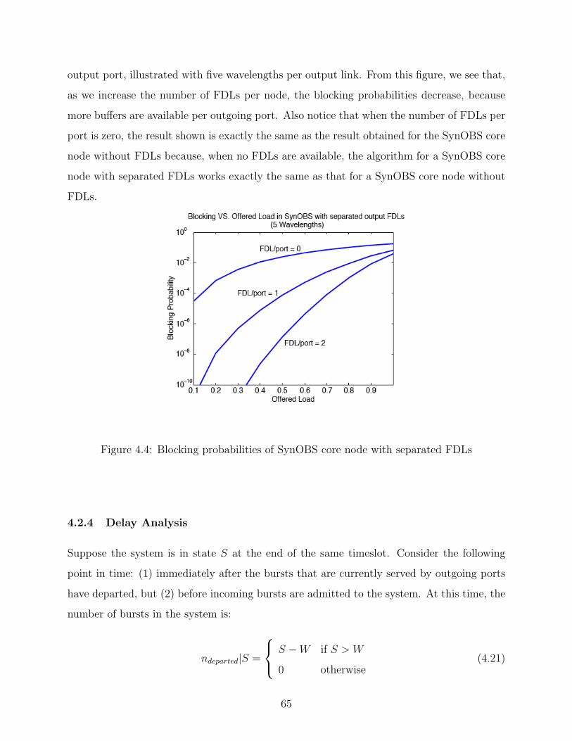
output port, illustrated with five wavelengths per output link. From this figure, we see that,
as we increase the number of FDLs per node, the blocking probabilities decrease, because
more buffers are available per outgoing port. Also notice that when the number of FDLs per
port is zero, the result shown is exactly the same as the result obtained for the SynOBS core
node without FDLs because, when no FDLs are available, the algorithm for a SynOBS core
node with separated FDLs works exactly the same as that for a SynOBS core node without
FDLs.
Figure 4.4: Blocking probabilities of SynOBS core node with separated FDLs
4.2.4 Delay Analysis
Suppose the system is in state S at the end of the same timeslot. Consider the following
point in time: (1) immediately after the bursts that are currently served by outgoing ports
have departed, but (2) before incoming bursts are admitted to the system. At this time, the
number of bursts in the system is:
ndeparted|S =
S −W if S > W
0 otherwise(4.21)
65
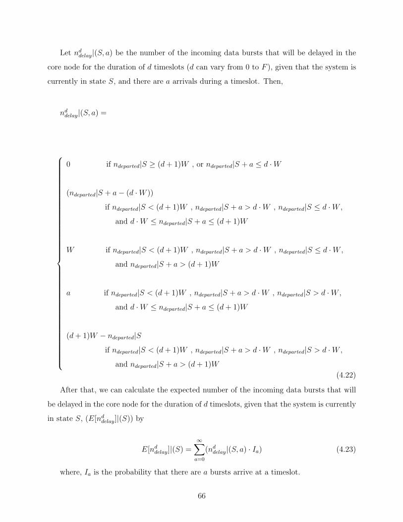
Let nddelay|(S, a) be the number of the incoming data bursts that will be delayed in the
core node for the duration of d timeslots (d can vary from 0 to F ), given that the system is
currently in state S, and there are a arrivals during a timeslot. Then,
nddelay|(S, a) =
0 if ndeparted|S ≥ (d+ 1)W , or ndeparted|S + a ≤ d ·W
(ndeparted|S + a− (d ·W ))
if ndeparted|S < (d+ 1)W , ndeparted|S + a > d ·W , ndeparted|S ≤ d ·W ,
and d ·W ≤ ndeparted|S + a ≤ (d+ 1)W
W if ndeparted|S < (d+ 1)W , ndeparted|S + a > d ·W , ndeparted|S ≤ d ·W ,
and ndeparted|S + a > (d+ 1)W
a if ndeparted|S < (d+ 1)W , ndeparted|S + a > d ·W , ndeparted|S > d ·W ,
and d ·W ≤ ndeparted|S + a ≤ (d+ 1)W
(d+ 1)W − ndeparted|S
if ndeparted|S < (d+ 1)W , ndeparted|S + a > d ·W , ndeparted|S > d ·W ,
and ndeparted|S + a > (d+ 1)W
(4.22)
After that, we can calculate the expected number of the incoming data bursts that will
be delayed in the core node for the duration of d timeslots, given that the system is currently
in state S, (E[nddelay]|(S)) by
E[nddelay]|(S) =∞∑a=0
(nddelay|(S, a) · Ia) (4.23)
where, Ia is the probability that there are a bursts arrive at a timeslot.
66
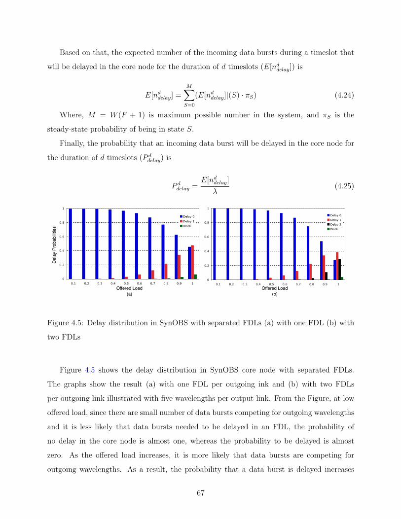
Based on that, the expected number of the incoming data bursts during a timeslot that
will be delayed in the core node for the duration of d timeslots (E[nddelay]) is
E[nddelay] =M∑S=0
(E[nddelay]|(S) · πS) (4.24)
Where, M = W (F + 1) is maximum possible number in the system, and πS is the
steady-state probability of being in state S.
Finally, the probability that an incoming data burst will be delayed in the core node for
the duration of d timeslots (P ddelay) is
P ddelay =
E[nddelay]
λ(4.25)
0
0.2
0.4
0.6
0.8
1
0.1 0.2 0.3 0.4 0.5 0.6 0.7 0.8 0.9 1
Delay 0
Delay 1
Block
0
0.2
0.4
0.6
0.8
1
0.1 0.2 0.3 0.4 0.5 0.6 0.7 0.8 0.9 1
Delay 0
Delay 1
Delay 2
Block
(a) (b)Offered Load
Dela
y Pr
obab
ilitie
s
Offered Load
Figure 4.5: Delay distribution in SynOBS with separated FDLs (a) with one FDL (b) with
two FDLs
Figure 4.5 shows the delay distribution in SynOBS core node with separated FDLs.
The graphs show the result (a) with one FDL per outgoing ink and (b) with two FDLs
per outgoing link illustrated with five wavelengths per output link. From the Figure, at low
offered load, since there are small number of data bursts competing for outgoing wavelengths
and it is less likely that data bursts needed to be delayed in an FDL, the probability of
no delay in the core node is almost one, whereas the probability to be delayed is almost
zero. As the offered load increases, it is more likely that data bursts are competing for
outgoing wavelengths. As a result, the probability that a data burst is delayed increases
67
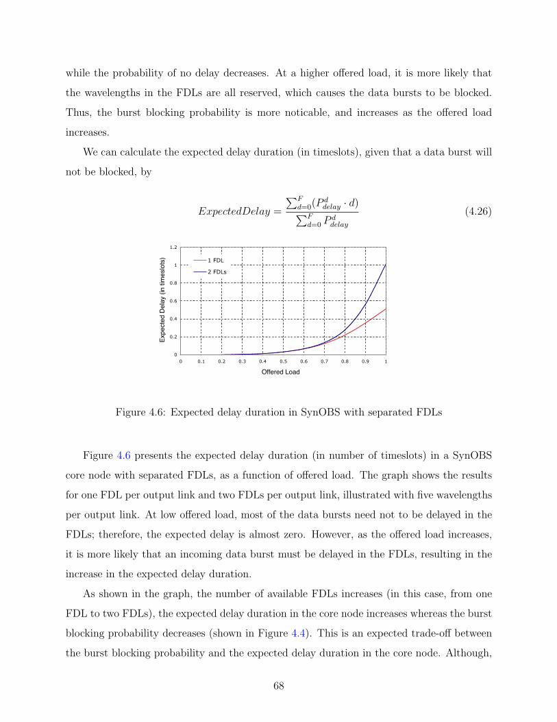
while the probability of no delay decreases. At a higher offered load, it is more likely that
the wavelengths in the FDLs are all reserved, which causes the data bursts to be blocked.
Thus, the burst blocking probability is more noticable, and increases as the offered load
increases.
We can calculate the expected delay duration (in timeslots), given that a data burst will
not be blocked, by
ExpectedDelay =
∑Fd=0(P
ddelay · d)∑F
d=0 Pddelay
(4.26)
0
0.2
0.4
0.6
0.8
1
1.2
0 0.1 0.2 0.3 0.4 0.5 0.6 0.7 0.8 0.9 1
1 FDL
2 FDLs
Offered Load
Expe
cted
Del
ay (i
n tim
eslo
ts)
Figure 4.6: Expected delay duration in SynOBS with separated FDLs
Figure 4.6 presents the expected delay duration (in number of timeslots) in a SynOBS
core node with separated FDLs, as a function of offered load. The graph shows the results
for one FDL per output link and two FDLs per output link, illustrated with five wavelengths
per output link. At low offered load, most of the data bursts need not to be delayed in the
FDLs; therefore, the expected delay is almost zero. However, as the offered load increases,
it is more likely that an incoming data burst must be delayed in the FDLs, resulting in the
increase in the expected delay duration.
As shown in the graph, the number of available FDLs increases (in this case, from one
FDL to two FDLs), the expected delay duration in the core node increases whereas the burst
blocking probability decreases (shown in Figure 4.4). This is an expected trade-off between
the burst blocking probability and the expected delay duration in the core node. Although,
68
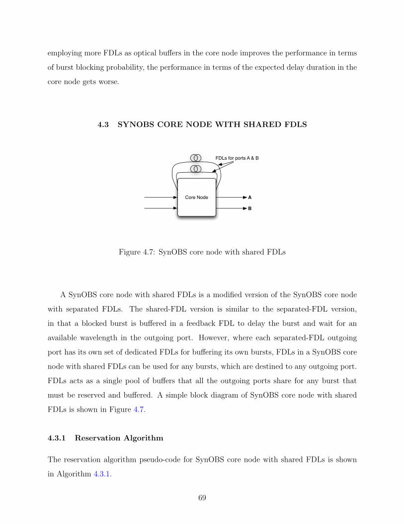
employing more FDLs as optical buffers in the core node improves the performance in terms
of burst blocking probability, the performance in terms of the expected delay duration in the
core node gets worse.
4.3 SYNOBS CORE NODE WITH SHARED FDLS
Core Node
FDLs for ports A & B
A
B
Figure 4.7: SynOBS core node with shared FDLs
A SynOBS core node with shared FDLs is a modified version of the SynOBS core node
with separated FDLs. The shared-FDL version is similar to the separated-FDL version,
in that a blocked burst is buffered in a feedback FDL to delay the burst and wait for an
available wavelength in the outgoing port. However, where each separated-FDL outgoing
port has its own set of dedicated FDLs for buffering its own bursts, FDLs in a SynOBS core
node with shared FDLs can be used for any bursts, which are destined to any outgoing port.
FDLs acts as a single pool of buffers that all the outgoing ports share for any burst that
must be reserved and buffered. A simple block diagram of SynOBS core node with shared
FDLs is shown in Figure 4.7.
4.3.1 Reservation Algorithm
The reservation algorithm pseudo-code for SynOBS core node with shared FDLs is shown
in Algorithm 4.3.1.
69
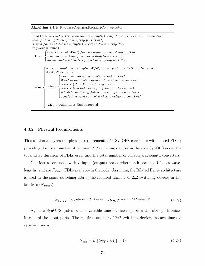
Algorithm 4.3.1: ProcessControlPacket(ControPacket)
read Control Packet for incoming wavelength (Win), timeslot (Tin), and destinationlookup Routing Table for outgoing port (Pout)search for available wavelength (Wout) in Pout during T inif (Wout is found)
then
reserve (Pout, Wout) for incoming data burst during T inschedule switching fabric according to reservationupdate and send control packet to outgoing port Pout
else
search available wavelength (Wfdl) in every shared FDLs in the nodeif (Wfdl is found)
then
Tavai← nearest available timslot in PoutWout← available wavelength in Pout during Tavaireserve (Pout, Wout) during Tavaireserve timeslots in Wfdl from Tin to Tvai− 1schedule switching fabric according to reservationsupdate and send control packet to outgoing port Pout
else{comment: Burst dropped
4.3.2 Physical Requirements
This section analyzes the physical requirements of a SynOBS core node with shared FDLs;
providing the total number of required 2x2 switching devices in the core SynOBS node, the
total delay duration of FDLs used, and the total number of tunable wavelength converters.
Consider a core node with L input (output) ports, where each port has W data wave-
lengths, and are Fshared FDLs available in the node. Assuming the Dilated Benes architecture
is used in the space switching fabric, the required number of 2x2 switching devices in the
fabric is (NBenes):
NBenes = 2 · 2dlog2(W (L+Fshared))e · log2(2dlog2(W (L+Fshared))e) (4.27)
Again, a SynOBS system with a variable timeslot size requires a timeslot synchronizer
in each of the input ports. The required number of 2x2 switching devices in each timeslot
synchronizer is
Nsyn = L(dlog2(T/A)e+ 1) (4.28)
70
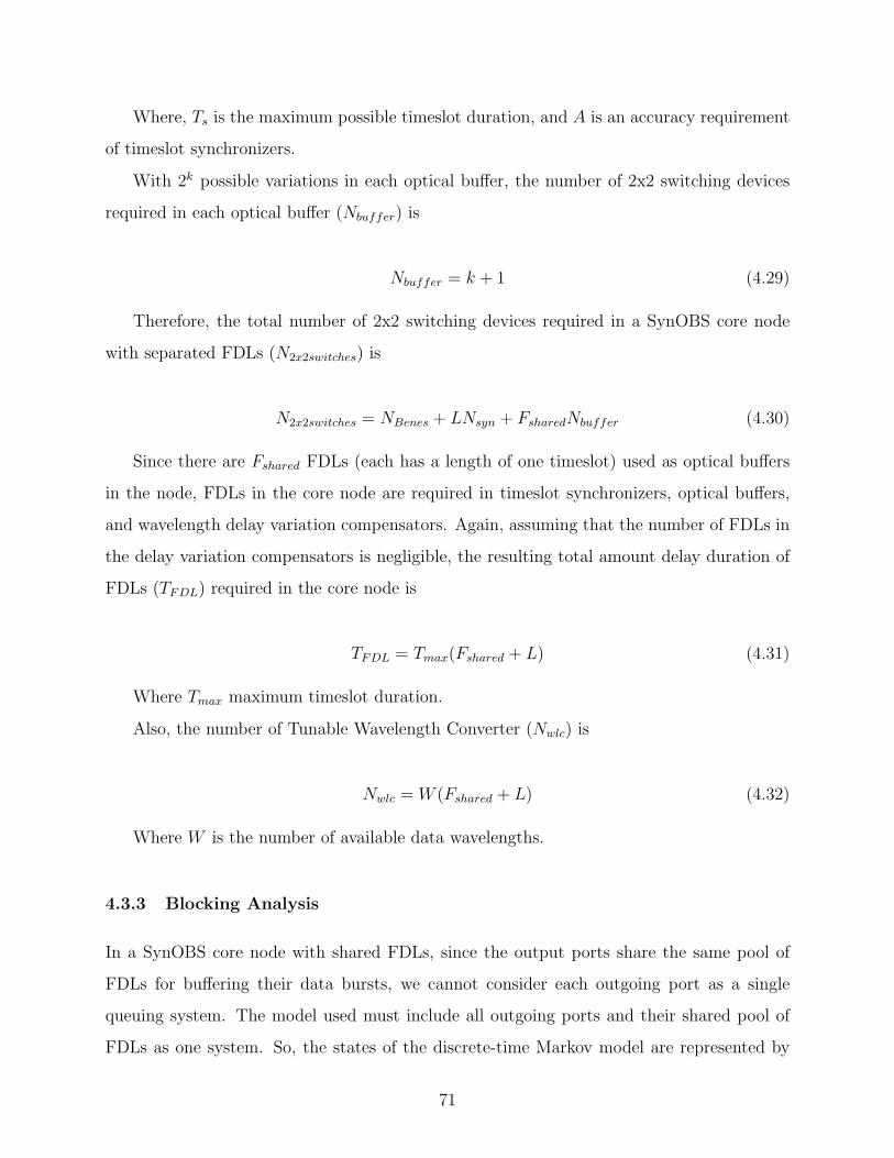
Where, Ts is the maximum possible timeslot duration, and A is an accuracy requirement
of timeslot synchronizers.
With 2k possible variations in each optical buffer, the number of 2x2 switching devices
required in each optical buffer (Nbuffer) is
Nbuffer = k + 1 (4.29)
Therefore, the total number of 2x2 switching devices required in a SynOBS core node
with separated FDLs (N2x2switches) is
N2x2switches = NBenes + LNsyn + FsharedNbuffer (4.30)
Since there are Fshared FDLs (each has a length of one timeslot) used as optical buffers
in the node, FDLs in the core node are required in timeslot synchronizers, optical buffers,
and wavelength delay variation compensators. Again, assuming that the number of FDLs in
the delay variation compensators is negligible, the resulting total amount delay duration of
FDLs (TFDL) required in the core node is
TFDL = Tmax(Fshared + L) (4.31)
Where Tmax maximum timeslot duration.
Also, the number of Tunable Wavelength Converter (Nwlc) is
Nwlc = W (Fshared + L) (4.32)
Where W is the number of available data wavelengths.
4.3.3 Blocking Analysis
In a SynOBS core node with shared FDLs, since the output ports share the same pool of
FDLs for buffering their data bursts, we cannot consider each outgoing port as a single
queuing system. The model used must include all outgoing ports and their shared pool of
FDLs as one system. So, the states of the discrete-time Markov model are represented by
71
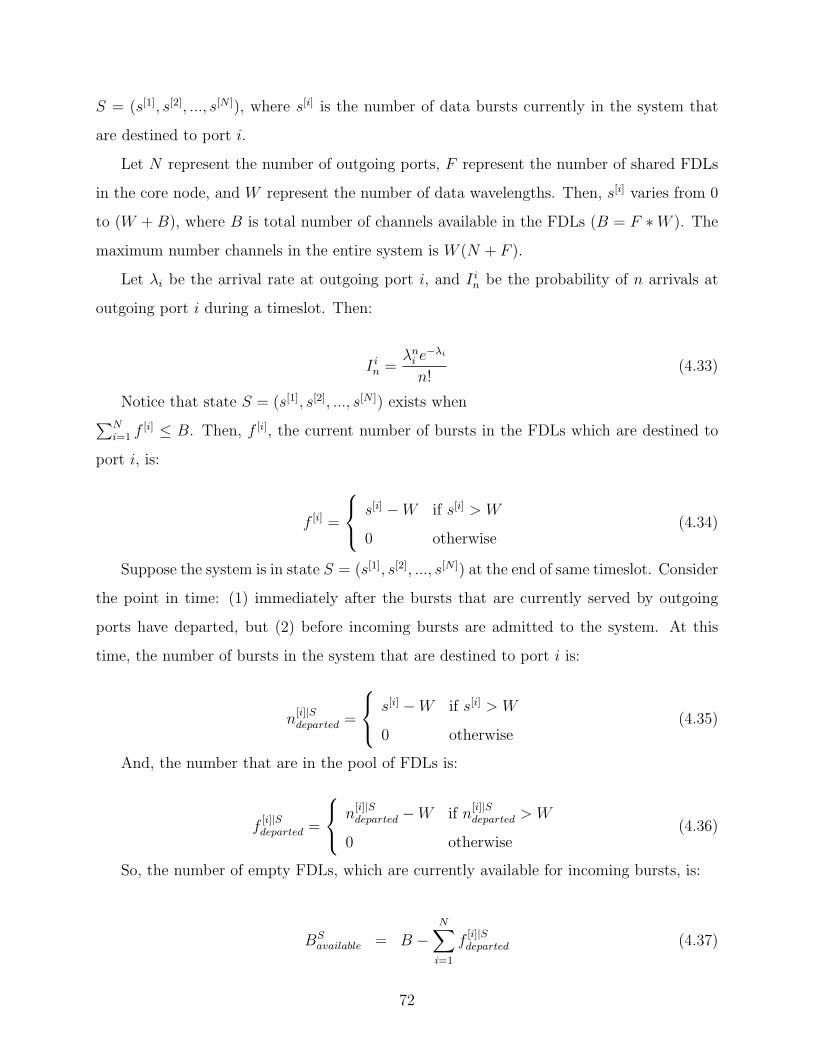
S = (s[1], s[2], ..., s[N ]), where s[i] is the number of data bursts currently in the system that
are destined to port i.
Let N represent the number of outgoing ports, F represent the number of shared FDLs
in the core node, and W represent the number of data wavelengths. Then, s[i] varies from 0
to (W +B), where B is total number of channels available in the FDLs (B = F ∗W ). The
maximum number channels in the entire system is W (N + F ).
Let λi be the arrival rate at outgoing port i, and I in be the probability of n arrivals at
outgoing port i during a timeslot. Then:
I in =λni e
−λi
n!(4.33)
Notice that state S = (s[1], s[2], ..., s[N ]) exists when∑Ni=1 f
[i] ≤ B. Then, f [i], the current number of bursts in the FDLs which are destined to
port i, is:
f [i] =
s[i] −W if s[i] > W
0 otherwise(4.34)
Suppose the system is in state S = (s[1], s[2], ..., s[N ]) at the end of same timeslot. Consider
the point in time: (1) immediately after the bursts that are currently served by outgoing
ports have departed, but (2) before incoming bursts are admitted to the system. At this
time, the number of bursts in the system that are destined to port i is:
n[i]|Sdeparted =
s[i] −W if s[i] > W
0 otherwise(4.35)
And, the number that are in the pool of FDLs is:
f[i]|Sdeparted =
n[i]|Sdeparted −W if n
[i]|Sdeparted > W
0 otherwise(4.36)
So, the number of empty FDLs, which are currently available for incoming bursts, is:
BSavailable = B −
N∑i=1
f[i]|Sdeparted (4.37)
72
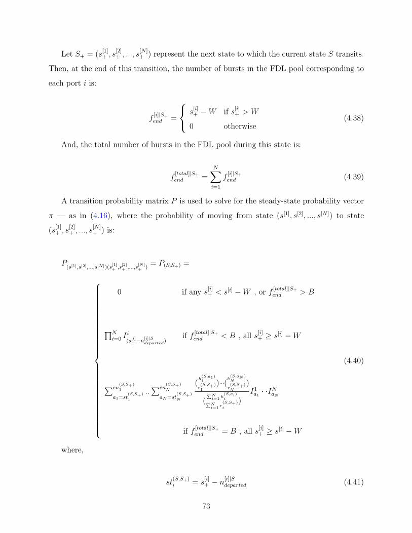
Let S+ = (s[1]+ , s
[2]+ , ..., s
[N ]+ ) represent the next state to which the current state S transits.
Then, at the end of this transition, the number of bursts in the FDL pool corresponding to
each port i is:
f[i]|S+
end =
s[i]+ −W if s
[i]+ > W
0 otherwise(4.38)
And, the total number of bursts in the FDL pool during this state is:
f[total]|S+
end =N∑i=1
f[i]|S+
end (4.39)
A transition probability matrix P is used to solve for the steady-state probability vector
π — as in (4.16), where the probability of moving from state (s[1], s[2], ..., s[N ]) to state
(s[1]+ , s
[2]+ , ..., s
[N ]+ ) is:
P(s[1],s[2],...,s[N ])(s
[1]+ ,s
[2]+ ,...,s
[N ]+ )
= P(S,S+) =
0 if any s[i]+ < s[i] −W , or f
[total]|S+
end > B
∏Ni=0 I
i
(s[i]+−n
[i]|Sdeparted)
if f[total]|S+
end < B , all s[i]+ ≥ s[i] −W
∑en(S,S+)
1
a1=st(S,S+)
1
..∑en
(S,S+)
N
aN=st(S,S+)
N
(h(S,a1)1
r(S,S+)
1
)···(h(S,aN )N
r(S,S+)
N
)
(PNi=1
h(S,ai)iPN
i=1r(S,S+)
i
)I1a1· ·INaN
if f[total]|S+
end = B , all s[i]+ ≥ s[i] −W
(4.40)
where,
st(S,S+)i = s
[i]+ − n
[i]|Sdeparted (4.41)
73
en(S,S+)i =
s[i]+ − n
[i]|Sdeparted if s
[i]+ < W
∞ otherwise(4.42)
h(S,a)i =
0 if s[i]+ < W
a if s[i]+ ≥ W , n
[i]|Sdeparted ≥ W
a− (W − n[i]|Sdeparted) if s
[i]+ ≥ W , n
[i]|Sdeparted < W
(4.43)
r(S,S+)i =
0 if s[i]+ < W
s[i]+ − n
[i]|Sdeparted if s
[i]+ ≥ W , n
[i]|Sdeparted ≥ W
s[i]+ −W if s
[i]+ ≥ W , n
[i]|Sdeparted < W
(4.44)
Immediately after bursts depart from the server, the number of incoming bursts that
correspond to each outgoing port is (a1, a2, ..., aN) = A, where ai represents the number
of arrivals for port i. So, the number of incoming bursts destined to port i that must be
buffered in the FDL pool is:
n[i]|(S,A)toFDL =
ai if n[i]|Sdeparted ≥ W
ai − (W − n[i]|Sdeparted) if n
[i]|Sdeparted < W , ai > W − n[i]|S
departed
0 if n[i]|Sdeparted < W , ai ≤ W − n[i]|S
departed
(4.45)
Then, the total number of incoming bursts that must be buffered in the FDL pool is:
n[total]|(S,A)toFDL =
N∑i=1
n[i]|(S,A)toFDL (4.46)
74
If the system is currently in state S = (s[1], s[2], ..., s[N ]) and the number of bursts arriving
at each outgoing port is (a1, a2, ..., aN) = A, then the number of blocked bursts is:
n(S,A)block =
n
[total]|(S,A)toFDL −BS
available if n[total]|(S,A)toFDL > BS
available
0 otherwise
(4.47)
So, if the system is in state S = (s[1], s[2], ..., s[N ]), the expected number of blocked bursts
during the next transition is:
E[nblock]|(S) =∞∑a1=0
∞∑a2=0
...
∞∑aN=0
(n
(S,A)block I
1a1I2a2· · · INaN
)(4.48)
And, the total expected number of blocked bursts in the system during each timeslot is:
E[nblock] =∑
(all S)
(πS · E[nblock]|(S)
)(4.49)
Then, the probability that an arriving burst will be blocked (Pb) is obtained by:
Pb =E[nblock]∑N
i=1 λi(4.50)
Figure 4.8 illustrates the blocking performance with respect to the offered load in a
SynOBS core node with shared FDLs, for various numbers of shared FDLs in the core
node. Again, the result is shown for five wavelengths per output link. Similarly to the
previous result of the SynOBS core node with separated FDLs, when the number of shared
FDLs is zero, the outcome is also exactly the same as the result obtained from a SynOBS
core node without FDLs. Reasonably, this occurs because, when no FDL is available in a
SynOBS core node with shared FDLs, its algorithm works exactly like that in a SynOBS core
node without FDLs. When the number of shared FDLs increases, the blocking probability
decreases because more optical buffers are available to handle the blocked traffic.
Figure 4.9 shows the result of calculating the burst blocking probability of a SynOBS
core node with shared FDLs with unbalanced offered load. In the core node, there are
75
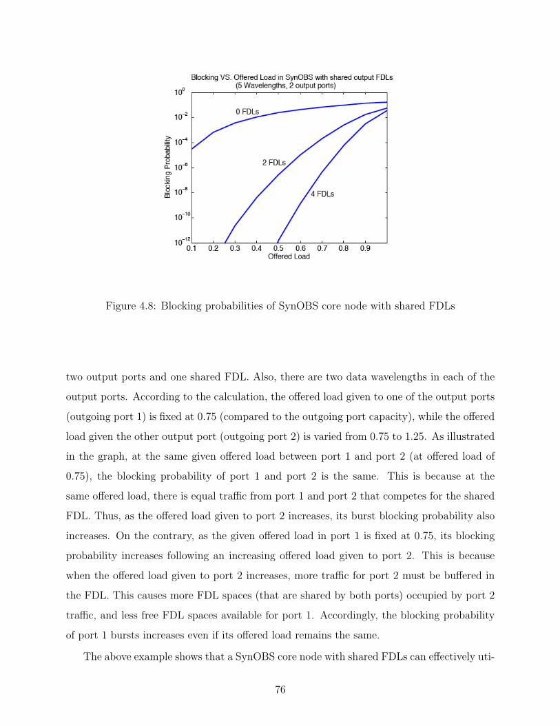
Figure 4.8: Blocking probabilities of SynOBS core node with shared FDLs
two output ports and one shared FDL. Also, there are two data wavelengths in each of the
output ports. According to the calculation, the offered load given to one of the output ports
(outgoing port 1) is fixed at 0.75 (compared to the outgoing port capacity), while the offered
load given the other output port (outgoing port 2) is varied from 0.75 to 1.25. As illustrated
in the graph, at the same given offered load between port 1 and port 2 (at offered load of
0.75), the blocking probability of port 1 and port 2 is the same. This is because at the
same offered load, there is equal traffic from port 1 and port 2 that competes for the shared
FDL. Thus, as the offered load given to port 2 increases, its burst blocking probability also
increases. On the contrary, as the given offered load in port 1 is fixed at 0.75, its blocking
probability increases following an increasing offered load given to port 2. This is because
when the offered load given to port 2 increases, more traffic for port 2 must be buffered in
the FDL. This causes more FDL spaces (that are shared by both ports) occupied by port 2
traffic, and less free FDL spaces available for port 1. Accordingly, the blocking probability
of port 1 bursts increases even if its offered load remains the same.
The above example shows that a SynOBS core node with shared FDLs can effectively uti-
76
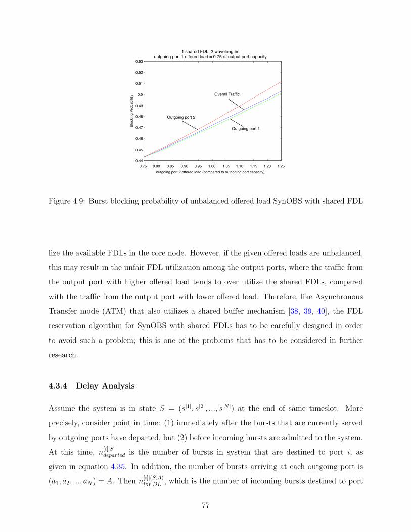
1 2 3 4 5 6 7 8 9 10 110.44
0.45
0.46
0.47
0.48
0.49
0.5
0.51
0.52
0.53Blocking VS. Offered Load in SynOBS with shared output FDLs (5 Wavelengths)
Blo
ckin
g P
roba
bili
ty
Offered Load0.75 0.80 0.85 0.90 0.95 1.00 1.05 1.10 1.15 1.20 1.25
Outgoing port 1
Outgoing port 2
Overall Traffic
1 shared FDL, 2 wavelengthsoutgoing port 1 offered load = 0.75 of output port capacity
outgoing port 2 offered load (compared to outgoging port capacity)
Figure 4.9: Burst blocking probability of unbalanced offered load SynOBS with shared FDL
lize the available FDLs in the core node. However, if the given offered loads are unbalanced,
this may result in the unfair FDL utilization among the output ports, where the traffic from
the output port with higher offered load tends to over utilize the shared FDLs, compared
with the traffic from the output port with lower offered load. Therefore, like Asynchronous
Transfer mode (ATM) that also utilizes a shared buffer mechanism [38, 39, 40], the FDL
reservation algorithm for SynOBS with shared FDLs has to be carefully designed in order
to avoid such a problem; this is one of the problems that has to be considered in further
research.
4.3.4 Delay Analysis
Assume the system is in state S = (s[1], s[2], ..., s[N ]) at the end of same timeslot. More
precisely, consider point in time: (1) immediately after the bursts that are currently served
by outgoing ports have departed, but (2) before incoming bursts are admitted to the system.
At this time, n[i]|Sdeparted is the number of bursts in system that are destined to port i, as
given in equation 4.35. In addition, the number of bursts arriving at each outgoing port is
(a1, a2, ..., aN) = A. Then n[i]|(S,A)toFDL , which is the number of incoming bursts destined to port
77
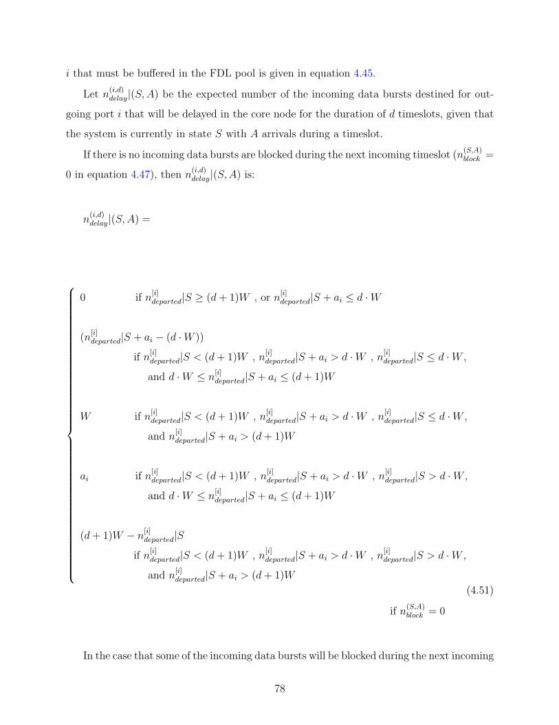
i that must be buffered in the FDL pool is given in equation 4.45.
Let n(i,d)delay|(S,A) be the expected number of the incoming data bursts destined for out-
going port i that will be delayed in the core node for the duration of d timeslots, given that
the system is currently in state S with A arrivals during a timeslot.
If there is no incoming data bursts are blocked during the next incoming timeslot (n(S,A)block =
0 in equation 4.47), then n(i,d)delay|(S,A) is:
n(i,d)delay|(S,A) =
0 if n[i]departed|S ≥ (d+ 1)W , or n
[i]departed|S + ai ≤ d ·W
(n[i]departed|S + ai − (d ·W ))
if n[i]departed|S < (d+ 1)W , n
[i]departed|S + ai > d ·W , n
[i]departed|S ≤ d ·W ,
and d ·W ≤ n[i]departed|S + ai ≤ (d+ 1)W
W if n[i]departed|S < (d+ 1)W , n
[i]departed|S + ai > d ·W , n
[i]departed|S ≤ d ·W ,
and n[i]departed|S + ai > (d+ 1)W
ai if n[i]departed|S < (d+ 1)W , n
[i]departed|S + ai > d ·W , n
[i]departed|S > d ·W ,
and d ·W ≤ n[i]departed|S + ai ≤ (d+ 1)W
(d+ 1)W − n[i]departed|S
if n[i]departed|S < (d+ 1)W , n
[i]departed|S + ai > d ·W , n
[i]departed|S > d ·W ,
and n[i]departed|S + ai > (d+ 1)W if n
(S,A)block = 0
(4.51)
if n(S,A)block = 0
In the case that some of the incoming data bursts will be blocked during the next incoming
78
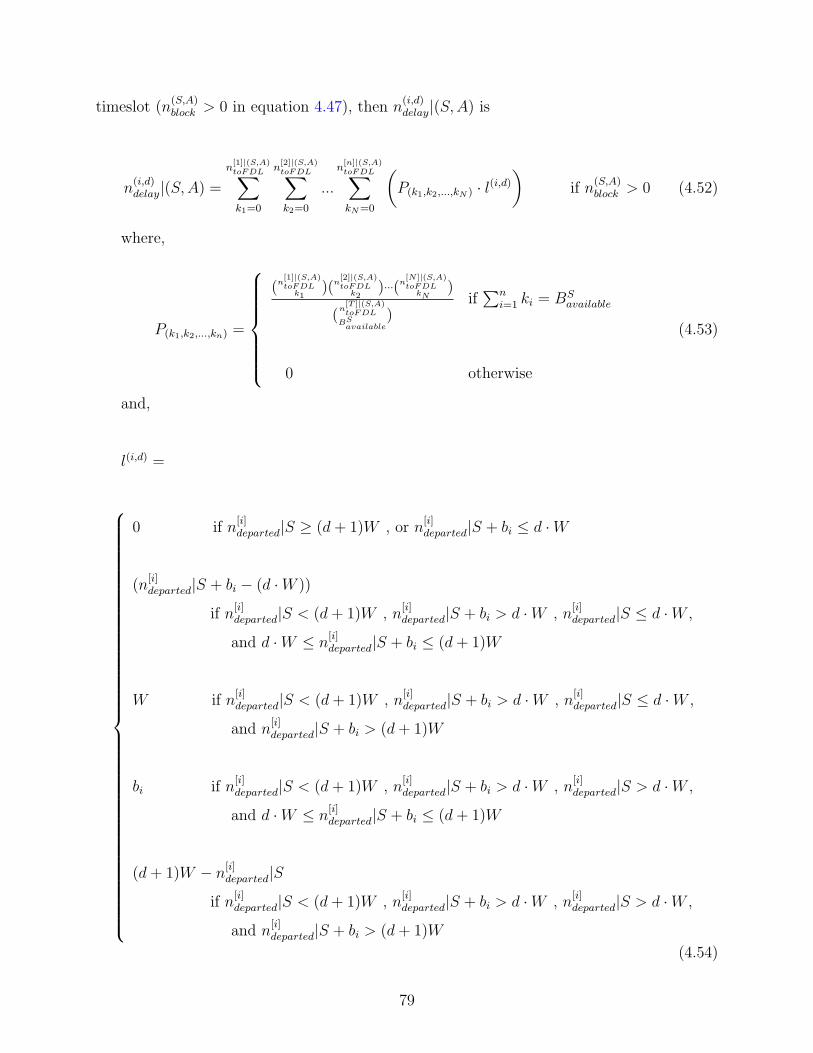
timeslot (n(S,A)block > 0 in equation 4.47), then n
(i,d)delay|(S,A) is
n(i,d)delay|(S,A) =
n[1]|(S,A)toFDL∑k1=0
n[2]|(S,A)toFDL∑k2=0
...
n[n]|(S,A)toFDL∑kN=0
(P(k1,k2,...,kN ) · l(i,d)
)if n
(S,A)block > 0 (4.52)
where,
P(k1,k2,...,kn) =
(n[1]|(S,A)toFDLk1
)(n[2]|(S,A)toFDLk2
)···(n[N ]|(S,A)toFDLkN
)
(n[T ]|(S,A)toFDL
BSavailable
)if∑n
i=1 ki = BSavailable
0 otherwise
(4.53)
and,
l(i,d) =
0 if n[i]departed|S ≥ (d+ 1)W , or n
[i]departed|S + bi ≤ d ·W
(n[i]departed|S + bi − (d ·W ))
if n[i]departed|S < (d+ 1)W , n
[i]departed|S + bi > d ·W , n
[i]departed|S ≤ d ·W ,
and d ·W ≤ n[i]departed|S + bi ≤ (d+ 1)W
W if n[i]departed|S < (d+ 1)W , n
[i]departed|S + bi > d ·W , n
[i]departed|S ≤ d ·W ,
and n[i]departed|S + bi > (d+ 1)W
bi if n[i]departed|S < (d+ 1)W , n
[i]departed|S + bi > d ·W , n
[i]departed|S > d ·W ,
and d ·W ≤ n[i]departed|S + bi ≤ (d+ 1)W
(d+ 1)W − n[i]departed|S
if n[i]departed|S < (d+ 1)W , n
[i]departed|S + bi > d ·W , n
[i]departed|S > d ·W ,
and n[i]departed|S + bi > (d+ 1)W
(4.54)
79
where,
bi = ai − (n[i]toFDL|(S,A)− ki) (4.55)
As a result, we can calculate the expected number of the incoming data bursts destined
for port i that will be delayed in the core node for a duration of d timeslots, given that the
system is currently in state S, (E[n(i,d)delay]|(S)) by
E[n(i,d)delay]|(S) =
∞∑a1=0
∞∑a2=0
...∞∑
aN=0
((n
(i,d)delay|(S,A))I1
a1I2a2· · · INaN
)(4.56)
Where I iai is the probability that there are ai bursts arriving for outgoing port i during
a timeslot.
Based on this equation, the expected number of the incoming data bursts during a
timeslot destined for port i that will be delayed in the core node for a duration of d timeslots
(E[n(i,d)delay]) is
E[n(i,d)delay] =
∑all S
(E[n
(i,d)delay]|(S) · πS
)(4.57)
Therefore, the probability of an incoming data burst destined for port i that will be
delayed in the core node for a duration of d timeslots (P(i,d)delay) is
P(i,d)delay =
E[n(i,d)delay]
λi(4.58)
Finally, the probability of an incoming data burst will be delayed in the core node for
the duration of d timeslots (P ddelay) is
P ddelay =
∑Ni=1E[n
(i,d)delay]∑N
i=1 λi(4.59)
Figure 4.10 shows the delay distribution in a SynOBS core node with shared FDLs. The
graphs present results for (a) one shared FDL and (b) two shared FDLs, illustrated with five
wavelengths per output link with two outgoing ports. Similarly to the result of a SynOBS
core node with separated FDLs, at low offered load, the probability of no delay in the core
node is almost one while the probability to be delayed is almost zero. When the offered
80
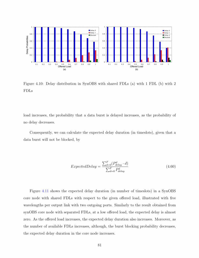
0
0.2
0.4
0.6
0.8
1
0.1 0.2 0.3 0.4 0.5 0.6 0.7 0.8 0.9 1
Delay 0
Delay 1
Delay 2
Blocked
0
0.2
0.4
0.6
0.8
1
0.1 0.2 0.3 0.4 0.5 0.6 0.7 0.8 0.9 1
Delay 0
Delay 1
Blocked
(a) (b)Offered Load
Dela
y Pr
obab
ilitie
s
Offered Load
Figure 4.10: Delay distribution in SynOBS with shared FDLs (a) with 1 FDL (b) with 2
FDLs
load increases, the probability that a data burst is delayed increases, as the probability of
no delay decreases.
Consequently, we can calculate the expected delay duration (in timeslots), given that a
data burst will not be blocked, by
ExpectedDelay =
∑Fd=0(P
ddelay · d)∑F
d=0 Pddelay
(4.60)
Figure 4.11 shows the expected delay duration (in number of timeslots) in a SynOBS
core node with shared FDLs with respect to the given offered load, illustrated with five
wavelengths per output link with two outgoing ports. Similarly to the result obtained from
synOBS core node with separated FDLs, at a low offered load, the expected delay is almost
zero. As the offered load increases, the expected delay duration also increases. Moreover, as
the number of available FDLs increases, although, the burst blocking probability decreases,
the expected delay duration in the core node increases.
81
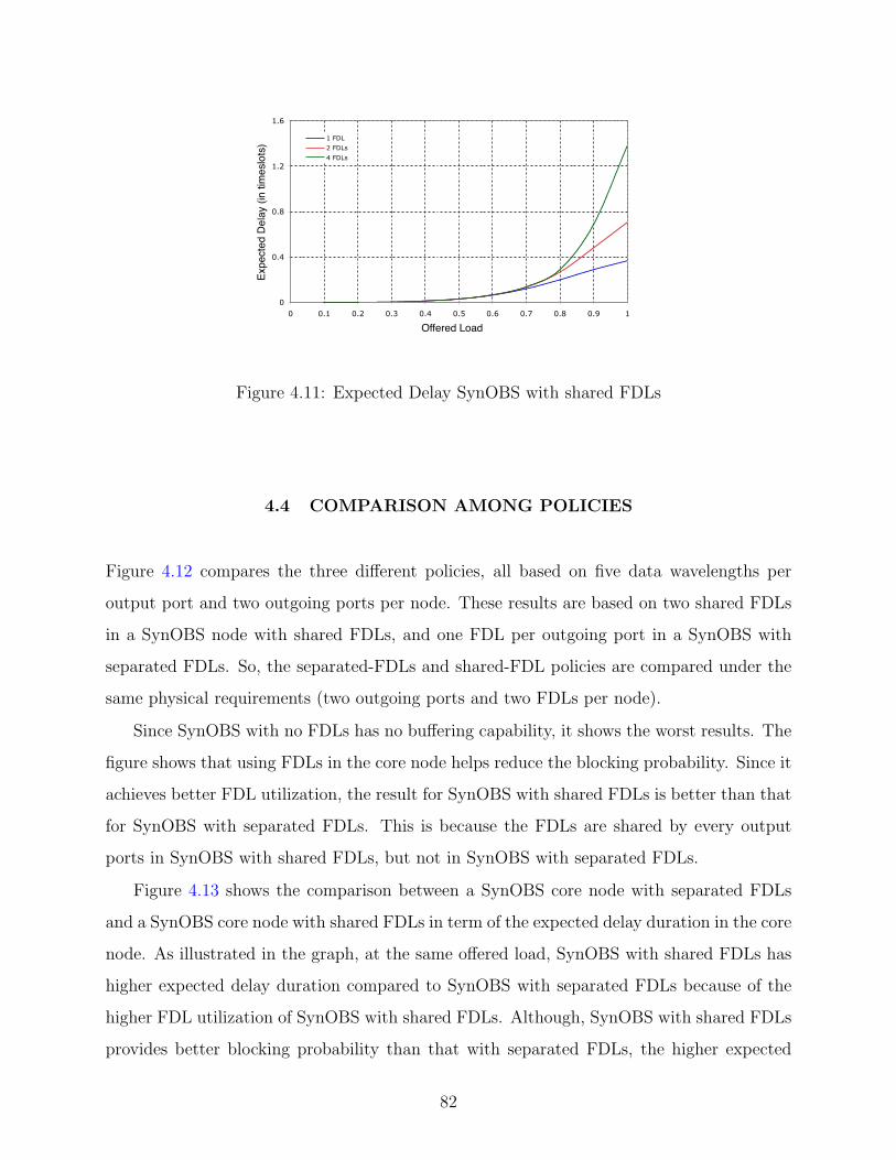
0
0.4
0.8
1.2
1.6
0 0.1 0.2 0.3 0.4 0.5 0.6 0.7 0.8 0.9 1
1 FDL
2 FDLs
4 FDLs
Offered Load
Expe
cted
Del
ay (i
n tim
eslo
ts)
Figure 4.11: Expected Delay SynOBS with shared FDLs
4.4 COMPARISON AMONG POLICIES
Figure 4.12 compares the three different policies, all based on five data wavelengths per
output port and two outgoing ports per node. These results are based on two shared FDLs
in a SynOBS node with shared FDLs, and one FDL per outgoing port in a SynOBS with
separated FDLs. So, the separated-FDLs and shared-FDL policies are compared under the
same physical requirements (two outgoing ports and two FDLs per node).
Since SynOBS with no FDLs has no buffering capability, it shows the worst results. The
figure shows that using FDLs in the core node helps reduce the blocking probability. Since it
achieves better FDL utilization, the result for SynOBS with shared FDLs is better than that
for SynOBS with separated FDLs. This is because the FDLs are shared by every output
ports in SynOBS with shared FDLs, but not in SynOBS with separated FDLs.
Figure 4.13 shows the comparison between a SynOBS core node with separated FDLs
and a SynOBS core node with shared FDLs in term of the expected delay duration in the core
node. As illustrated in the graph, at the same offered load, SynOBS with shared FDLs has
higher expected delay duration compared to SynOBS with separated FDLs because of the
higher FDL utilization of SynOBS with shared FDLs. Although, SynOBS with shared FDLs
provides better blocking probability than that with separated FDLs, the higher expected
82
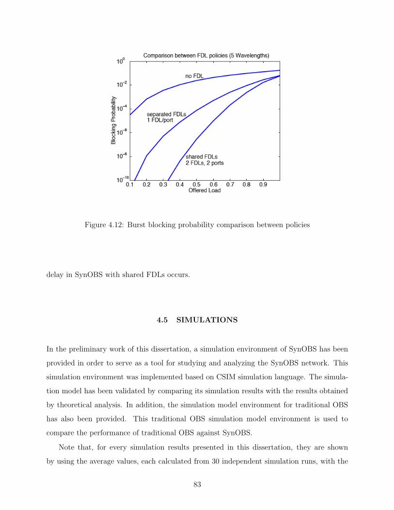
Figure 4.12: Burst blocking probability comparison between policies
delay in SynOBS with shared FDLs occurs.
4.5 SIMULATIONS
In the preliminary work of this dissertation, a simulation environment of SynOBS has been
provided in order to serve as a tool for studying and analyzing the SynOBS network. This
simulation environment was implemented based on CSIM simulation language. The simula-
tion model has been validated by comparing its simulation results with the results obtained
by theoretical analysis. In addition, the simulation model environment for traditional OBS
has also been provided. This traditional OBS simulation model environment is used to
compare the performance of traditional OBS against SynOBS.
Note that, for every simulation results presented in this dissertation, they are shown
by using the average values, each calculated from 30 independent simulation runs, with the
83
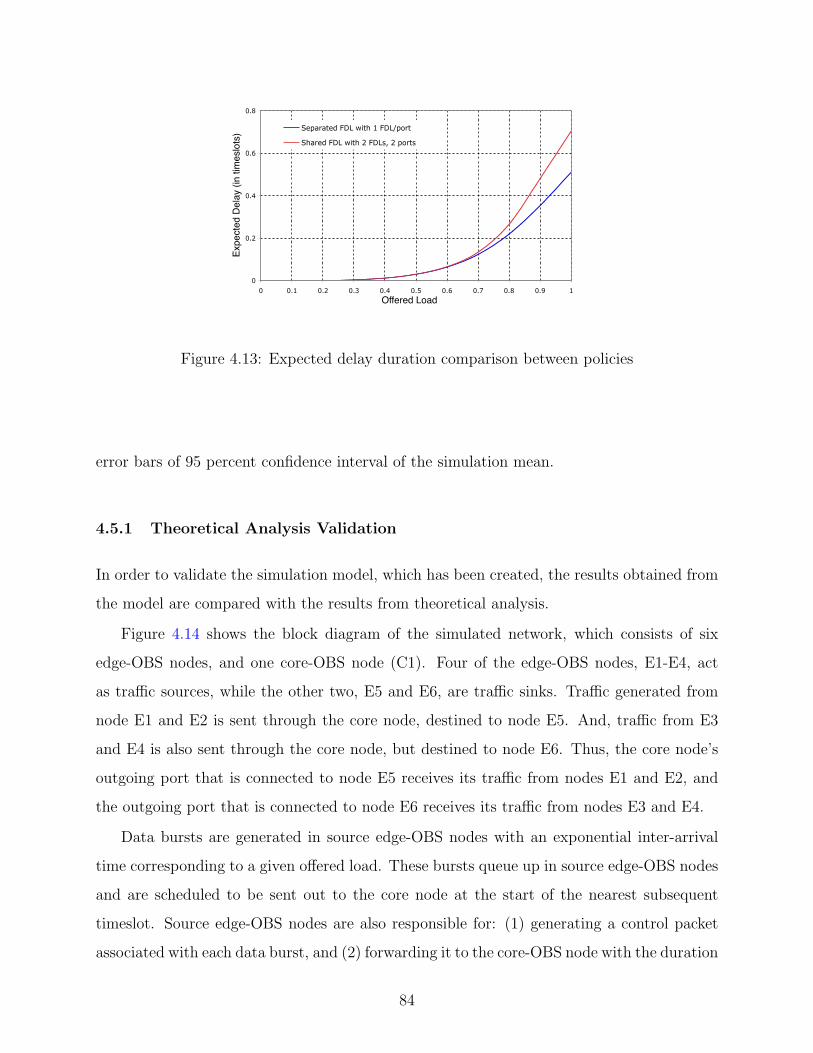
0
0.2
0.4
0.6
0.8
0 0.1 0.2 0.3 0.4 0.5 0.6 0.7 0.8 0.9 1
Separated FDL with 1 FDL/port
Shared FDL with 2 FDLs, 2 ports
Offered Load
Expe
cted
Del
ay (i
n tim
eslo
ts)
Figure 4.13: Expected delay duration comparison between policies
error bars of 95 percent confidence interval of the simulation mean.
4.5.1 Theoretical Analysis Validation
In order to validate the simulation model, which has been created, the results obtained from
the model are compared with the results from theoretical analysis.
Figure 4.14 shows the block diagram of the simulated network, which consists of six
edge-OBS nodes, and one core-OBS node (C1). Four of the edge-OBS nodes, E1-E4, act
as traffic sources, while the other two, E5 and E6, are traffic sinks. Traffic generated from
node E1 and E2 is sent through the core node, destined to node E5. And, traffic from E3
and E4 is also sent through the core node, but destined to node E6. Thus, the core node’s
outgoing port that is connected to node E5 receives its traffic from nodes E1 and E2, and
the outgoing port that is connected to node E6 receives its traffic from nodes E3 and E4.
Data bursts are generated in source edge-OBS nodes with an exponential inter-arrival
time corresponding to a given offered load. These bursts queue up in source edge-OBS nodes
and are scheduled to be sent out to the core node at the start of the nearest subsequent
timeslot. Source edge-OBS nodes are also responsible for: (1) generating a control packet
associated with each data burst, and (2) forwarding it to the core-OBS node with the duration
84
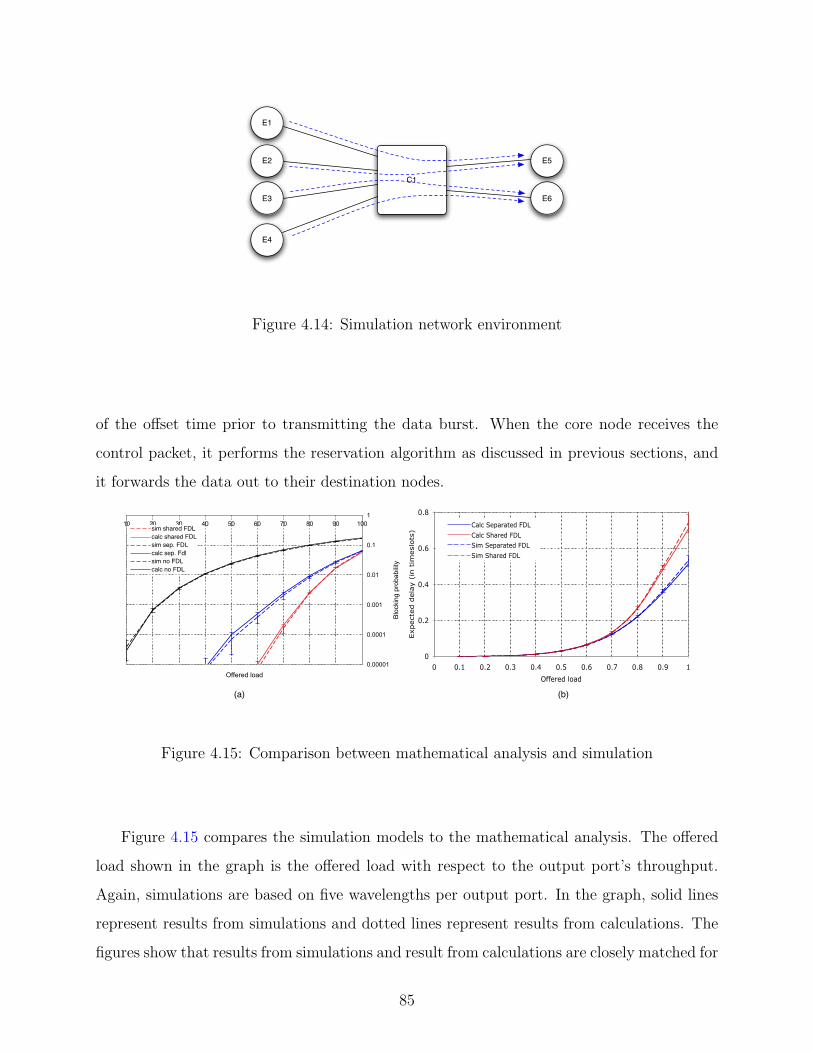
E1
E2
E3
E5
E6
E4
C1
Figure 4.14: Simulation network environment
of the offset time prior to transmitting the data burst. When the core node receives the
control packet, it performs the reservation algorithm as discussed in previous sections, and
it forwards the data out to their destination nodes.
0.00001
0.0001
0.001
0.01
0.1
110 20 30 40 50 60 70 80 90 100
Offered load
Blo
ckin
g pr
obab
ility
sim shared FDLcalc shared FDLsim sep. FDLcalc sep. Fdlsim no FDLcalc no FDL
(a) (b)
0
0.2
0.4
0.6
0.8
0 0.1 0.2 0.3 0.4 0.5 0.6 0.7 0.8 0.9 1
Offered load
Expect
ed d
ela
y (
in t
imesl
ots
)
Calc Separated FDL
Calc Shared FDLSim Separated FDL
Sim Shared FDL
Figure 4.15: Comparison between mathematical analysis and simulation
Figure 4.15 compares the simulation models to the mathematical analysis. The offered
load shown in the graph is the offered load with respect to the output port’s throughput.
Again, simulations are based on five wavelengths per output port. In the graph, solid lines
represent results from simulations and dotted lines represent results from calculations. The
figures show that results from simulations and result from calculations are closely matched for
85
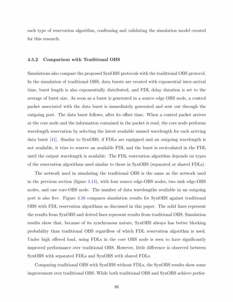
each type of reservation algorithm, confirming and validating the simulation model created
for this research.
4.5.2 Comparison with Traditional OBS
Simulations also compare the proposed SynOBS protocols with the traditional OBS protocol.
In the simulation of traditional OBS, data bursts are created with exponential inter-arrival
time, burst length is also exponentially distributed, and FDL delay duration is set to the
average of burst size. As soon as a burst is generated in a source edge OBS node, a control
packet associated with the data burst is immediately generated and sent out through the
outgoing port. The data burst follows, after its offset time. When a control packet arrives
at the core node and the information contained in the packet is read, the core node performs
wavelength reservation by selecting the latest available unused wavelength for each arriving
data burst [41]. Similar to SynOBS, if FDLs are equipped and an outgoing wavelength is
not available, it tries to reserve an available FDL and the burst is recirculated in the FDL
until the output wavelength is available. The FDL reservation algorithm depends on types
of the reservation algorithms used similar to those in SynOBS (separated or shared FDLs).
The network used in simulating the traditional OBS is the same as the network used
in the previous section (figure 4.14), with four source edge-OBS nodes, two sink edge-OBS
nodes, and one core-OBS node. The number of data wavelengths available in an outgoing
port is also five. Figure 4.16 compares simulation results for SynOBS against traditional
OBS with FDL reservation algorithms as discussed in this paper. The solid lines represent
the results from SynOBS and dotted lines represent results from traditional OBS. Simulation
results show that, because of its synchronous nature, SynOBS always has better blocking
probability than traditional OBS regardless of which FDL reservation algorithm is used.
Under high offered load, using FDLs in the core OBS node is seen to have significantly
improved performance over traditional OBS. However, little difference is observed between
SynOBS with separated FDLs and SynOBS with shared FDLs.
Comparing traditional OBS with SynOBS without FDLs, the SynOBS results show some
improvement over traditional OBS. While both traditional OBS and SynOBS achieve perfor-
86
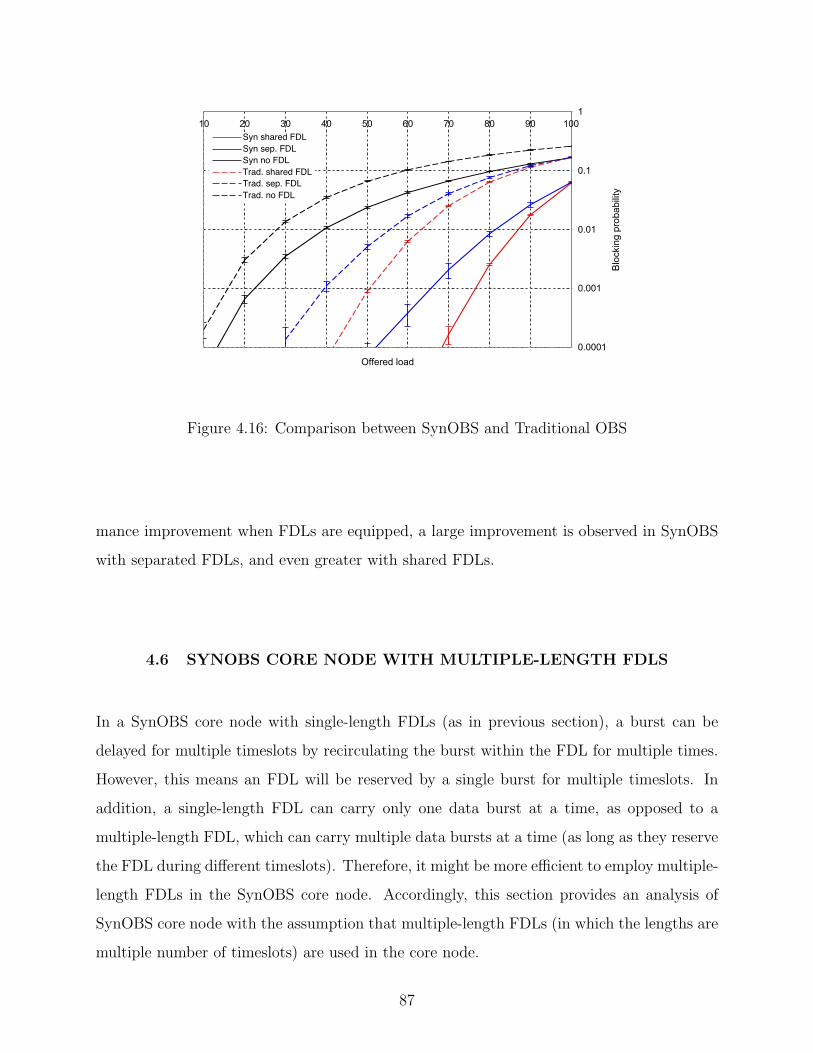
0.0001
0.001
0.01
0.1
110 20 30 40 50 60 70 80 90 100
Offered load
Blo
ckin
g pr
obab
ility
Syn shared FDLSyn sep. FDLSyn no FDLTrad. shared FDLTrad. sep. FDLTrad. no FDL
Figure 4.16: Comparison between SynOBS and Traditional OBS
mance improvement when FDLs are equipped, a large improvement is observed in SynOBS
with separated FDLs, and even greater with shared FDLs.
4.6 SYNOBS CORE NODE WITH MULTIPLE-LENGTH FDLS
In a SynOBS core node with single-length FDLs (as in previous section), a burst can be
delayed for multiple timeslots by recirculating the burst within the FDL for multiple times.
However, this means an FDL will be reserved by a single burst for multiple timeslots. In
addition, a single-length FDL can carry only one data burst at a time, as opposed to a
multiple-length FDL, which can carry multiple data bursts at a time (as long as they reserve
the FDL during different timeslots). Therefore, it might be more efficient to employ multiple-
length FDLs in the SynOBS core node. Accordingly, this section provides an analysis of
SynOBS core node with the assumption that multiple-length FDLs (in which the lengths are
multiple number of timeslots) are used in the core node.
87
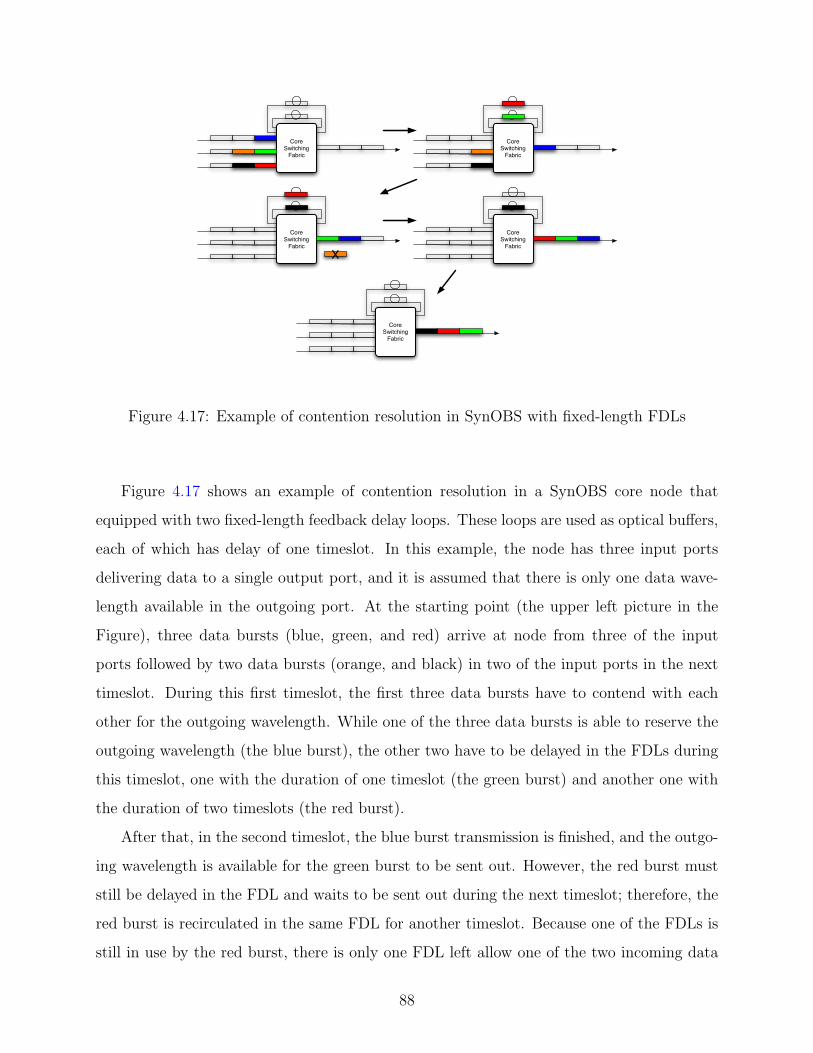
Core Switching
Fabric
Core Switching
Fabric
Core Switching
Fabric
Core Switching
Fabric
Core Switching
Fabric
X
Figure 4.17: Example of contention resolution in SynOBS with fixed-length FDLs
Figure 4.17 shows an example of contention resolution in a SynOBS core node that
equipped with two fixed-length feedback delay loops. These loops are used as optical buffers,
each of which has delay of one timeslot. In this example, the node has three input ports
delivering data to a single output port, and it is assumed that there is only one data wave-
length available in the outgoing port. At the starting point (the upper left picture in the
Figure), three data bursts (blue, green, and red) arrive at node from three of the input
ports followed by two data bursts (orange, and black) in two of the input ports in the next
timeslot. During this first timeslot, the first three data bursts have to contend with each
other for the outgoing wavelength. While one of the three data bursts is able to reserve the
outgoing wavelength (the blue burst), the other two have to be delayed in the FDLs during
this timeslot, one with the duration of one timeslot (the green burst) and another one with
the duration of two timeslots (the red burst).
After that, in the second timeslot, the blue burst transmission is finished, and the outgo-
ing wavelength is available for the green burst to be sent out. However, the red burst must
still be delayed in the FDL and waits to be sent out during the next timeslot; therefore, the
red burst is recirculated in the same FDL for another timeslot. Because one of the FDLs is
still in use by the red burst, there is only one FDL left allow one of the two incoming data
88
bursts to be delayed in the remaining FDL (the black burst), while the other one is blocked
and dropped (the orange burst).
In the third timeslot, the green burst transmission is finished, and the outgoing wave-
length is available for the red burst to be sent out but the black burst still must be recirculated
in an FDL and waits to be sent out during the next timeslot. Finally during the forth times-
lot, the red burst transmission is finished, and the outgoing wavelength is available for the
black burst to be sent out. At this point, in both of the FDLs, the core nodes are empty
and available all over again.
Core Switching
Fabric
Core Switching
Fabric
Core Switching
Fabric
Core Switching
Fabric
Core Switching
Fabric
Core Switching
Fabric
Figure 4.18: Example of contention resolution in SynOBS with multiple-length FDLs
Now, consider Figure 4.18. This Figure shows a similar core node configuration as in
Figure 4.17 discussed earlier, where there are three input ports sending data to a single
output port with one data wavelength available. Also, at the starting point (the upper left
picture in the Figure), the same set of data bursts arrive at the core node (three data bursts
(blue, green, and red) followed by two data bursts (orange, and black) in the next timeslot).
According to this Figure, what differs from the core node previously discussed in Figure
4.17 is that this time the core node is equipped with multiple-length feedback delay loops
(optical buffers), one with the delay duration of one timeslot, and another one with the delay
duration of two timeslots. Again, during the first timeslot, the first three data bursts have
89
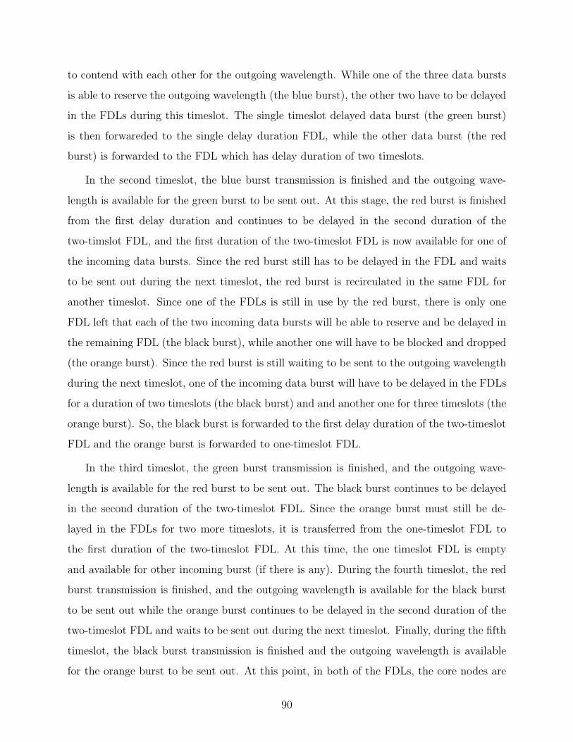
to contend with each other for the outgoing wavelength. While one of the three data bursts
is able to reserve the outgoing wavelength (the blue burst), the other two have to be delayed
in the FDLs during this timeslot. The single timeslot delayed data burst (the green burst)
is then forwareded to the single delay duration FDL, while the other data burst (the red
burst) is forwarded to the FDL which has delay duration of two timeslots.
In the second timeslot, the blue burst transmission is finished and the outgoing wave-
length is available for the green burst to be sent out. At this stage, the red burst is finished
from the first delay duration and continues to be delayed in the second duration of the
two-timslot FDL, and the first duration of the two-timeslot FDL is now available for one of
the incoming data bursts. Since the red burst still has to be delayed in the FDL and waits
to be sent out during the next timeslot, the red burst is recirculated in the same FDL for
another timeslot. Since one of the FDLs is still in use by the red burst, there is only one
FDL left that each of the two incoming data bursts will be able to reserve and be delayed in
the remaining FDL (the black burst), while another one will have to be blocked and dropped
(the orange burst). Since the red burst is still waiting to be sent to the outgoing wavelength
during the next timeslot, one of the incoming data burst will have to be delayed in the FDLs
for a duration of two timeslots (the black burst) and and another one for three timeslots (the
orange burst). So, the black burst is forwarded to the first delay duration of the two-timeslot
FDL and the orange burst is forwarded to one-timeslot FDL.
In the third timeslot, the green burst transmission is finished, and the outgoing wave-
length is available for the red burst to be sent out. The black burst continues to be delayed
in the second duration of the two-timeslot FDL. Since the orange burst must still be de-
layed in the FDLs for two more timeslots, it is transferred from the one-timeslot FDL to
the first duration of the two-timeslot FDL. At this time, the one timeslot FDL is empty
and available for other incoming burst (if there is any). During the fourth timeslot, the red
burst transmission is finished, and the outgoing wavelength is available for the black burst
to be sent out while the orange burst continues to be delayed in the second duration of the
two-timeslot FDL and waits to be sent out during the next timeslot. Finally, during the fifth
timeslot, the black burst transmission is finished and the outgoing wavelength is available
for the orange burst to be sent out. At this point, in both of the FDLs, the core nodes are
90
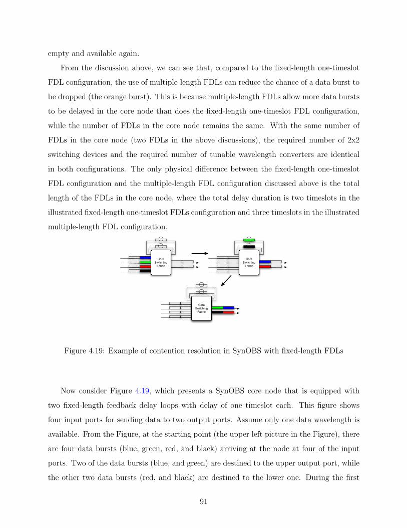
empty and available again.
From the discussion above, we can see that, compared to the fixed-length one-timeslot
FDL configuration, the use of multiple-length FDLs can reduce the chance of a data burst to
be dropped (the orange burst). This is because multiple-length FDLs allow more data bursts
to be delayed in the core node than does the fixed-length one-timeslot FDL configuration,
while the number of FDLs in the core node remains the same. With the same number of
FDLs in the core node (two FDLs in the above discussions), the required number of 2x2
switching devices and the required number of tunable wavelength converters are identical
in both configurations. The only physical difference between the fixed-length one-timeslot
FDL configuration and the multiple-length FDL configuration discussed above is the total
length of the FDLs in the core node, where the total delay duration is two timeslots in the
illustrated fixed-length one-timeslot FDLs configuration and three timeslots in the illustrated
multiple-length FDL configuration.
Core Switching
Fabric
Core Switching
Fabric
Core Switching
Fabric
Figure 4.19: Example of contention resolution in SynOBS with fixed-length FDLs
Now consider Figure 4.19, which presents a SynOBS core node that is equipped with
two fixed-length feedback delay loops with delay of one timeslot each. This figure shows
four input ports for sending data to two output ports. Assume only one data wavelength is
available. From the Figure, at the starting point (the upper left picture in the Figure), there
are four data bursts (blue, green, red, and black) arriving at the node at four of the input
ports. Two of the data bursts (blue, and green) are destined to the upper output port, while
the other two data bursts (red, and black) are destined to the lower one. During the first
91
timeslot, two of the incoming data bursts (blue, and green) have to compete with each other
for the outgoing wavelength in the upper output port, at the same time, the other two data
bursts (red, and black) have to compete for the outgoing wavelength in the lower port. In
this case, if the blue burst and the red burst successfully reserve their outgoing wavelengths,
they are forwarded to their respective outgoing ports; but the other two (green, and black)
are delayed in each of the two available FDLs to be sent out in next timeslot. Subsequently,
in the second timeslot, the blue burst and the red burst transmissions are completed, and
the outgoing wavelengths are available for the green and the black burst to be sent out. We
see that, after being delayed in FDLs, the green burst and the black one are delivered to
their outgoing ports immediately after the blue and the red burst, without any unnecessary
delay duration between the bursts.
Core Switching
Fabric
Core Switching
Fabric
Core Switching
Fabric
Core Switching
Fabric
Figure 4.20: Example of contention resolution in SynOBS with multiple-length FDLs
Now, look at Figure 4.20, which illustrates a SynOBS core node equipped with two
multiple-length feedback delay loops, one with delay of one timeslot and the other with two
timeslots. Again, there are four input ports sending data to two of the output ports, and it
is also assumed that there is only one data wavelength available. At the starting points (the
upper left picture in the Figure), four data bursts (blue, green, red, and black) arrive at the
node at four input ports. Two of the data bursts (blue, and green) are destined to the upper
output port while the other two data bursts (red, and black) are destined to the lower one.
During the first timeslot, two of the incoming data bursts (blue, and green) have to
compete with each other for the outgoing wavelength in the upper output port and the other
92
two data bursts (red, and black) have to compete for the outgoing wavelength in the lower
port. The blue burst and the red burst successfully reserve their outgoing wavelengths and
they are forwarded to their outgoing ports, but the other two (green, and black) have to be
delayed in the FDLs in order to be sent out in next timeslot. Both the green burst and the
black burst need to be delayed in FDLs and wait for their respective outgoing wavelengths
for only one timeslot. Since there is only one FDL that has a delay duration of one timeslot,
the other FDL has to be delayed for two timeslots. In order to avoid dropping a burst,
one of the data bursts has to be forwarded to the two-timeslot FDL. In this case, the black
burst succesfully reserves the one-timeslot FDL while the green burst has to be delayed in
the two-timeslot FDL. In this case, at the second timeslot, the blue burst and the red burst
transmissions are finished, and the outgoing wavelengths are available for the green and
the black burst to be sent out. Finishing its delay duration in its FDL, the black burst is
forwarded out to its outgoing port immediately after the red burst. But, since the green
burst is delayed in the two-timeslot FDL, it must continue being delayed in the FDL for
another timeslot before it can be sent out to the outgoing wavelength in the next timeslot
even though the required wavelength was available.
The discussions above show that, although using multiple-length FDLs configuration can
reduce the chance of a data burst to be dropped, in some cases, some data bursts may have
to be delayed in the FDLs with an unnecessarily longer duration. This is due to the fact
that the combinations in the delay durations of the available FDLs may not exactly match
the needed delay duration of an incoming data burst, causing the data burst to be delayed
longer. In the fixed-length one-timeslot FDL configuration, where every FDL has a length of
one timeslot, whenever an FDL is available for an incoming data burst, the data burst can
always be delayed in this FDL for the exact duration that the data burst needs. This can
be done by keep recirculating in the FDL with the same number of cycles as the number of
timeslots needed to be delayed.
93
4.6.1 Reservation Algorithm
This section describes the reservation algorithm which is used for analysis of SynOBS core
node with multiple-length FDLs.
Algorithm 4.6.1 shows the pseudo-code of a resource reservation algorithm for a Syn-
OBS code node with multiple-length FDLs. Initially, as a control packet arrives at a core
node in the control channel, the control packet is received and processed. After the infor-
mation is retrieved from the control packet, the routing algorithm determines the outgoing
port. The algorithm subsequently searches for an available wavelength in the outgoing port
during the incoming burst’s timeslot. If a wavelength is available, it is reserved for the
incoming data burst and then the core switching fabric connection schedule is updated.
However, if no wavelength is available, the algorithm then determines the nearest available
wavelength and timeslot in the outgoing port. After that, the algorithm invokes function
RecursiveFDLSearch() in order to search if there is any FDL combination that can delay
the data burst to the available outgoing timeslot. After the function RecursiveFDLSearch()
performs its FDL search, it returns with three possible state.
• First, if the search is successful (FoundMatch), the algorithm then reserves this outgoing
wavelength/timeslot and these FDLs in order to buffer the data burst until it is sent to
the outgoing port.
• Second, if the search fails, but there is an available combination of FDLs that delays the
data burst past that of the available outgoing timeslot (FDLTooLong), the algorithm will
check whether there is an available wavelength at the outgoing port during the timeslot
in which the burst will come out of the FDLs. If so, at this timeslot, the algorithm will
reserve this outgoing wavelength as well as these FDLs in order to buffer the data burst
until it is sent to the outgoing port during this available timeslot. On the other hand,
in the case that the outgoing port is not available, the algorithm will then determine
the next upcoming timeslot that has an available wavelength in its outgoing port, and
repeat RecursiveFDLSearch().
• Third, if the search is unsuccessful, and also there is no FDL configuration that can
delay the data burst longer than the available outgoing timeslot, the node cannot buffer
94
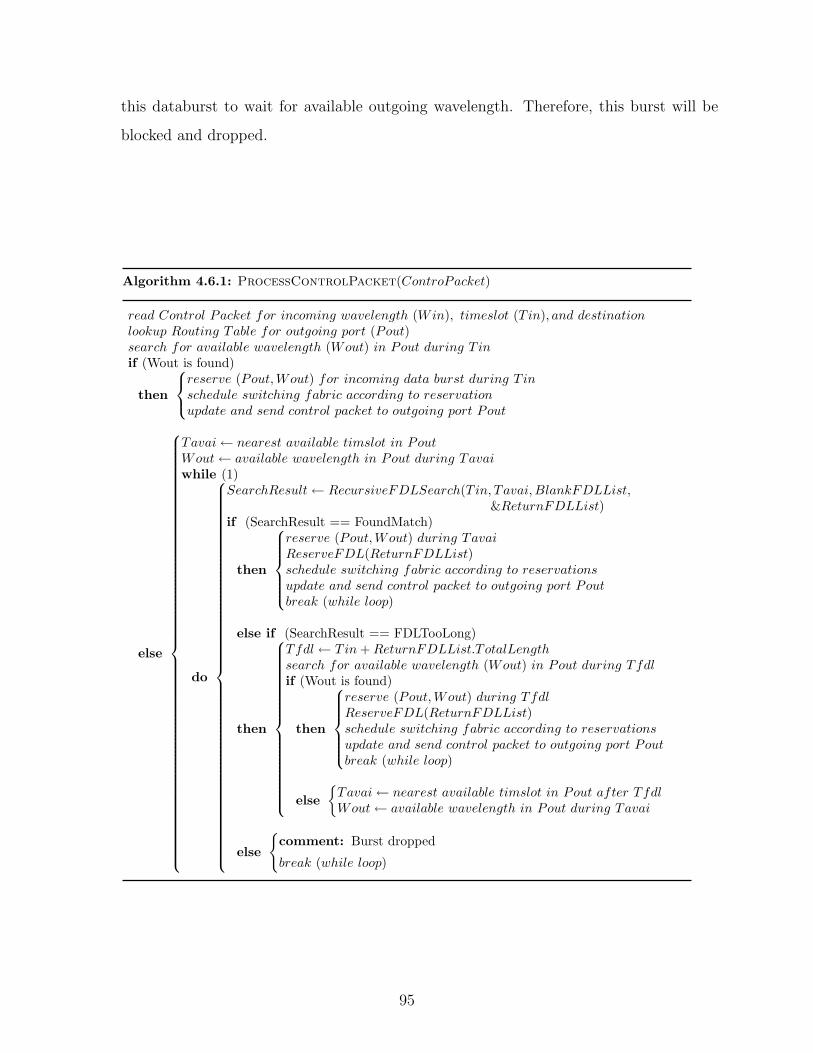
this databurst to wait for available outgoing wavelength. Therefore, this burst will be
blocked and dropped.
Algorithm 4.6.1: ProcessControlPacket(ControPacket)
read Control Packet for incoming wavelength (Win), timeslot (Tin), and destinationlookup Routing Table for outgoing port (Pout)search for available wavelength (Wout) in Pout during T inif (Wout is found)
then
reserve (Pout, Wout) for incoming data burst during T inschedule switching fabric according to reservationupdate and send control packet to outgoing port Pout
else
Tavai← nearest available timslot in PoutWout← available wavelength in Pout during Tavaiwhile (1)
do
SearchResult← RecursiveFDLSearch(Tin, Tavai, BlankFDLList,&ReturnFDLList)
if (SearchResult == FoundMatch)
then
reserve (Pout, Wout) during TavaiReserveFDL(ReturnFDLList)schedule switching fabric according to reservationsupdate and send control packet to outgoing port Poutbreak (while loop)
else if (SearchResult == FDLTooLong)
then
Tfdl← Tin + ReturnFDLList.TotalLengthsearch for available wavelength (Wout) in Pout during Tfdlif (Wout is found)
then
reserve (Pout, Wout) during TfdlReserveFDL(ReturnFDLList)schedule switching fabric according to reservationsupdate and send control packet to outgoing port Poutbreak (while loop)
else{
Tavai← nearest available timslot in Pout after TfdlWout← available wavelength in Pout during Tavai
else
{comment: Burst dropped
break (while loop)
95
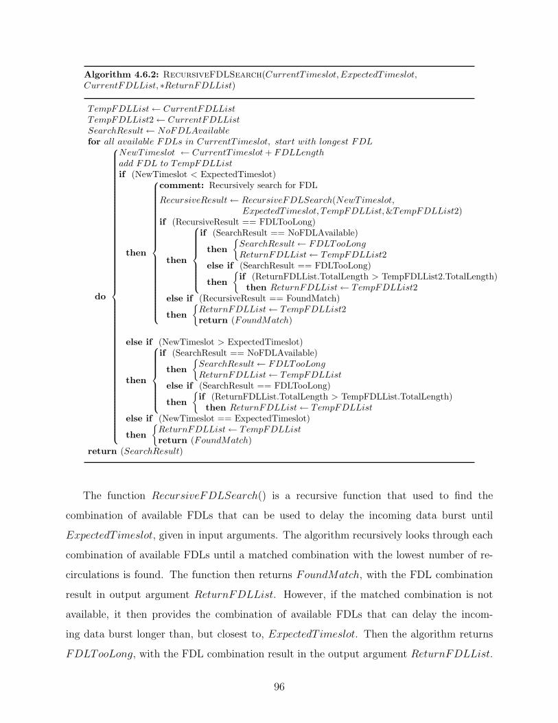
Algorithm 4.6.2: RecursiveFDLSearch(CurrentT imeslot, ExpectedT imeslot,CurrentFDLList, ∗ReturnFDLList)
TempFDLList← CurrentFDLListTempFDLList2← CurrentFDLListSearchResult← NoFDLAvailablefor all available FDLs in CurrentT imeslot, start with longest FDL
do
NewTimeslot ← CurrentT imeslot + FDLLengthadd FDL to TempFDLListif (NewTimeslot < ExpectedTimeslot)
then
comment: Recursively search for FDL
RecursiveResult← RecursiveFDLSearch(NewTimeslot,ExpectedT imeslot, TempFDLList, &TempFDLList2)
if (RecursiveResult == FDLTooLong)
then
if (SearchResult == NoFDLAvailable)
then{
SearchResult← FDLTooLongReturnFDLList← TempFDLList2
else if (SearchResult == FDLTooLong)
then{if (ReturnFDLList.TotalLength > TempFDLList2.TotalLength)then ReturnFDLList← TempFDLList2
else if (RecursiveResult == FoundMatch)
then{
ReturnFDLList← TempFDLList2return (FoundMatch)
else if (NewTimeslot > ExpectedTimeslot)
then
if (SearchResult == NoFDLAvailable)
then{
SearchResult← FDLTooLongReturnFDLList← TempFDLList
else if (SearchResult == FDLTooLong)
then{if (ReturnFDLList.TotalLength > TempFDLList.TotalLength)then ReturnFDLList← TempFDLList
else if (NewTimeslot == ExpectedTimeslot)
then{
ReturnFDLList← TempFDLListreturn (FoundMatch)
return (SearchResult)
The function RecursiveFDLSearch() is a recursive function that used to find the
combination of available FDLs that can be used to delay the incoming data burst until
ExpectedT imeslot, given in input arguments. The algorithm recursively looks through each
combination of available FDLs until a matched combination with the lowest number of re-
circulations is found. The function then returns FoundMatch, with the FDL combination
result in output argument ReturnFDLList. However, if the matched combination is not
available, it then provides the combination of available FDLs that can delay the incom-
ing data burst longer than, but closest to, ExpectedT imeslot. Then the algorithm returns
FDLTooLong, with the FDL combination result in the output argument ReturnFDLList.
96
In the worst case, if there is no available FDL combination that can delay the data burst
until ExpectedT imeslot or later than ExpectedT imeslot, then the algorithm returns with
NoFDLAvailable. The pseudo-code of the function RecursiveFDLSearch() is shown in
Algorithm 4.6.2.
4.6.2 Physical Requirements
This section provides the physical requirement analysis of a SynOBS core node with multiple-
length FDLs based on the total number of required 2x2 switching devices in the core SynOBS
node, the total delay duration of FDLs used, and the total number of tunable wavelength
converters.
Consider a core node with L input (output) ports, where each port has W data wave-
lengths, and F FDLs available in the node. Assuming the Dilated Benes architecture is used
in the space switching fabric, the required number of 2x2 switching devices in the fabric is
(NBenes):
NBenes = 2 · 2dlog2(W (L+F ))e · log2(2dlog2(W (L+F ))e) (4.61)
Again, a SynOBS system with variable timeslot size requires a timeslot synchronizer in
each of the input ports. The required number of 2x2 switching devices in each timeslot
synchronizer is
Nsyn = L(dlog2(Ts/A)e+ 1) (4.62)
Where, Ts is the maximum possible timeslot duration, and A is accuracy requirement of
timeslot synchronizers.
The number (Nbuffer) of 2x2 switching devices required in an optical buffer with 2k
variations is:
Nbuffer = k + 1 (4.63)
97
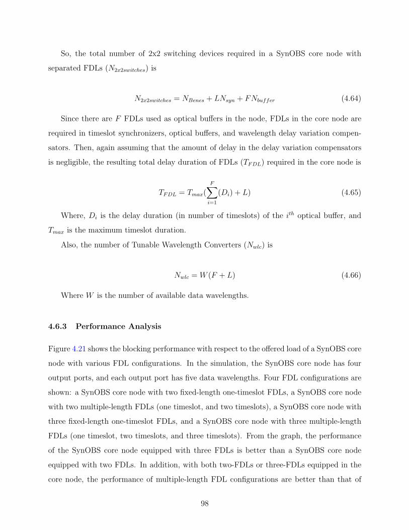
So, the total number of 2x2 switching devices required in a SynOBS core node with
separated FDLs (N2x2switches) is
N2x2switches = NBenes + LNsyn + FNbuffer (4.64)
Since there are F FDLs used as optical buffers in the node, FDLs in the core node are
required in timeslot synchronizers, optical buffers, and wavelength delay variation compen-
sators. Then, again assuming that the amount of delay in the delay variation compensators
is negligible, the resulting total delay duration of FDLs (TFDL) required in the core node is
TFDL = Tmax(F∑i=1
(Di) + L) (4.65)
Where, Di is the delay duration (in number of timeslots) of the ith optical buffer, and
Tmax is the maximum timeslot duration.
Also, the number of Tunable Wavelength Converters (Nwlc) is
Nwlc = W (F + L) (4.66)
Where W is the number of available data wavelengths.
4.6.3 Performance Analysis
Figure 4.21 shows the blocking performance with respect to the offered load of a SynOBS core
node with various FDL configurations. In the simulation, the SynOBS core node has four
output ports, and each output port has five data wavelengths. Four FDL configurations are
shown: a SynOBS core node with two fixed-length one-timeslot FDLs, a SynOBS core node
with two multiple-length FDLs (one timeslot, and two timeslots), a SynOBS core node with
three fixed-length one-timeslot FDLs, and a SynOBS core node with three multiple-length
FDLs (one timeslot, two timeslots, and three timeslots). From the graph, the performance
of the SynOBS core node equipped with three FDLs is better than a SynOBS core node
equipped with two FDLs. In addition, with both two-FDLs or three-FDLs equipped in the
core node, the performance of multiple-length FDL configurations are better than that of
98
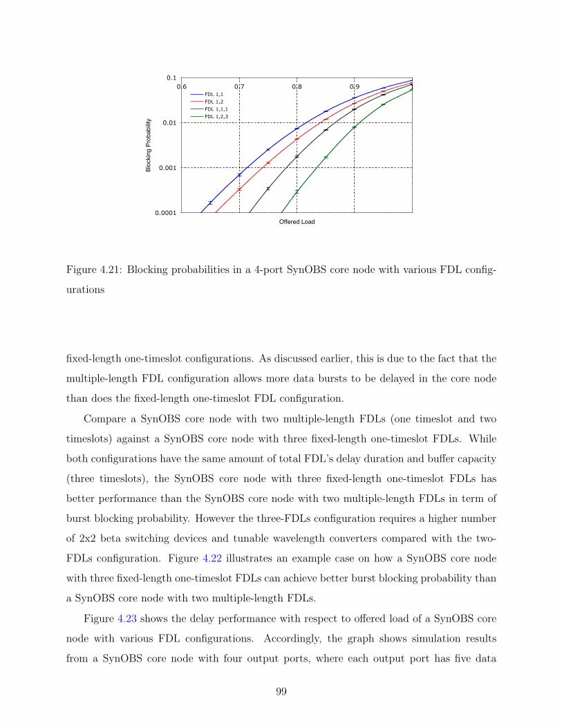
0.0001
0.001
0.01
0.10.6 0.7 0.8 0.9 1
Offered Load
Bloc
king
Prob
abilit
y
FDL 1,1
FDL 1,2
FDL 1,1,1
FDL 1,2,3
Figure 4.21: Blocking probabilities in a 4-port SynOBS core node with various FDL config-
urations
fixed-length one-timeslot configurations. As discussed earlier, this is due to the fact that the
multiple-length FDL configuration allows more data bursts to be delayed in the core node
than does the fixed-length one-timeslot FDL configuration.
Compare a SynOBS core node with two multiple-length FDLs (one timeslot and two
timeslots) against a SynOBS core node with three fixed-length one-timeslot FDLs. While
both configurations have the same amount of total FDL’s delay duration and buffer capacity
(three timeslots), the SynOBS core node with three fixed-length one-timeslot FDLs has
better performance than the SynOBS core node with two multiple-length FDLs in term of
burst blocking probability. However the three-FDLs configuration requires a higher number
of 2x2 beta switching devices and tunable wavelength converters compared with the two-
FDLs configuration. Figure 4.22 illustrates an example case on how a SynOBS core node
with three fixed-length one-timeslot FDLs can achieve better burst blocking probability than
a SynOBS core node with two multiple-length FDLs.
Figure 4.23 shows the delay performance with respect to offered load of a SynOBS core
node with various FDL configurations. Accordingly, the graph shows simulation results
from a SynOBS core node with four output ports, where each output port has five data
99
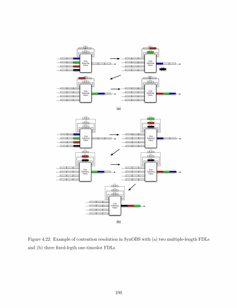
Core Switching
Fabric
Core Switching
Fabric
Core Switching
Fabric
Core Switching
Fabric
X
Core Switching
Fabric
Core Switching
Fabric
Core Switching
Fabric
Core Switching
Fabric
Core Switching
Fabric
(a)
(b)
Figure 4.22: Example of contention resolution in SynOBS with (a) two multiple-length FDLs
and (b) three fixed-legth one-timeslot FDLs
100
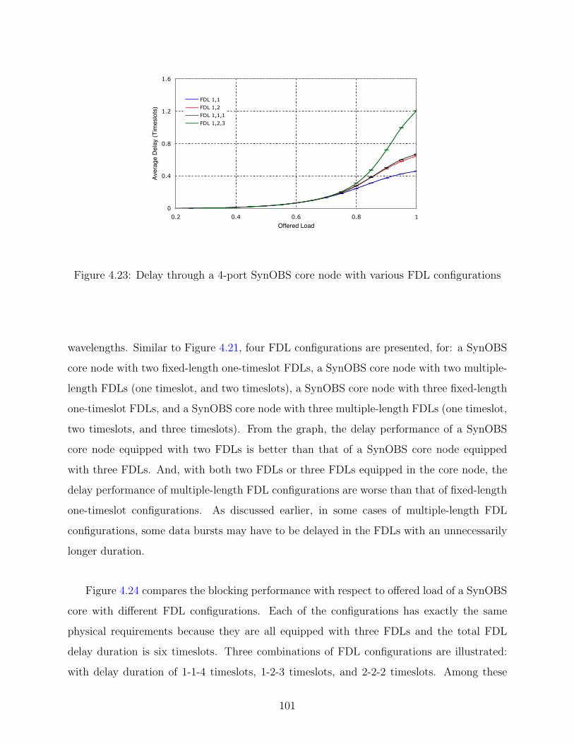
0
0.4
0.8
1.2
1.6
0.2 0.4 0.6 0.8 1
Offered Load
Aver
age
Dela
y (T
imes
lots
)
FDL 1,1
FDL 1,2
FDL 1,1,1
FDL 1,2,3
Figure 4.23: Delay through a 4-port SynOBS core node with various FDL configurations
wavelengths. Similar to Figure 4.21, four FDL configurations are presented, for: a SynOBS
core node with two fixed-length one-timeslot FDLs, a SynOBS core node with two multiple-
length FDLs (one timeslot, and two timeslots), a SynOBS core node with three fixed-length
one-timeslot FDLs, and a SynOBS core node with three multiple-length FDLs (one timeslot,
two timeslots, and three timeslots). From the graph, the delay performance of a SynOBS
core node equipped with two FDLs is better than that of a SynOBS core node equipped
with three FDLs. And, with both two FDLs or three FDLs equipped in the core node, the
delay performance of multiple-length FDL configurations are worse than that of fixed-length
one-timeslot configurations. As discussed earlier, in some cases of multiple-length FDL
configurations, some data bursts may have to be delayed in the FDLs with an unnecessarily
longer duration.
Figure 4.24 compares the blocking performance with respect to offered load of a SynOBS
core with different FDL configurations. Each of the configurations has exactly the same
physical requirements because they are all equipped with three FDLs and the total FDL
delay duration is six timeslots. Three combinations of FDL configurations are illustrated:
with delay duration of 1-1-4 timeslots, 1-2-3 timeslots, and 2-2-2 timeslots. Among these
101
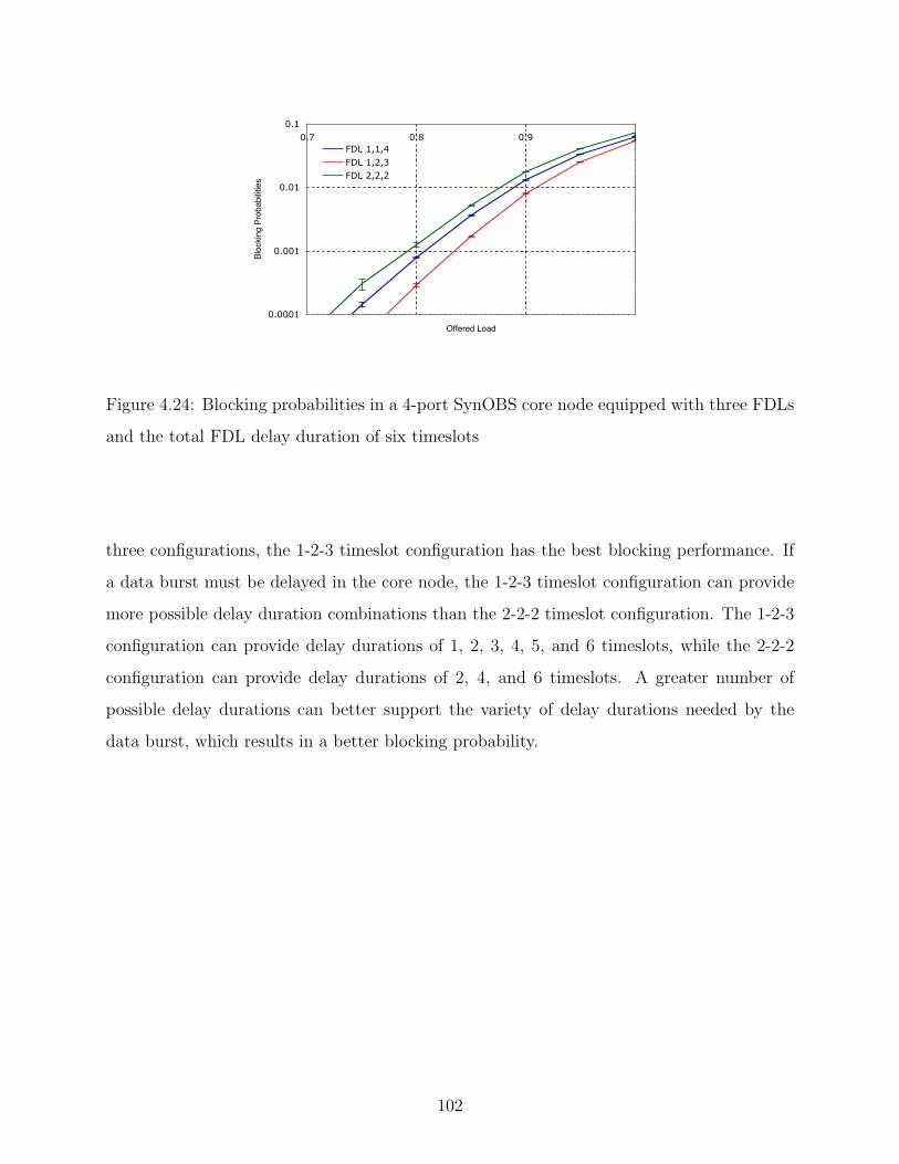
0.0001
0.001
0.01
0.10.7 0.8 0.9 1
Offered Load
Bloc
king
Prob
abilit
ies
FDL 1,1,4FDL 1,2,3FDL 2,2,2
Figure 4.24: Blocking probabilities in a 4-port SynOBS core node equipped with three FDLs
and the total FDL delay duration of six timeslots
three configurations, the 1-2-3 timeslot configuration has the best blocking performance. If
a data burst must be delayed in the core node, the 1-2-3 timeslot configuration can provide
more possible delay duration combinations than the 2-2-2 timeslot configuration. The 1-2-3
configuration can provide delay durations of 1, 2, 3, 4, 5, and 6 timeslots, while the 2-2-2
configuration can provide delay durations of 2, 4, and 6 timeslots. A greater number of
possible delay durations can better support the variety of delay durations needed by the
data burst, which results in a better blocking probability.
102
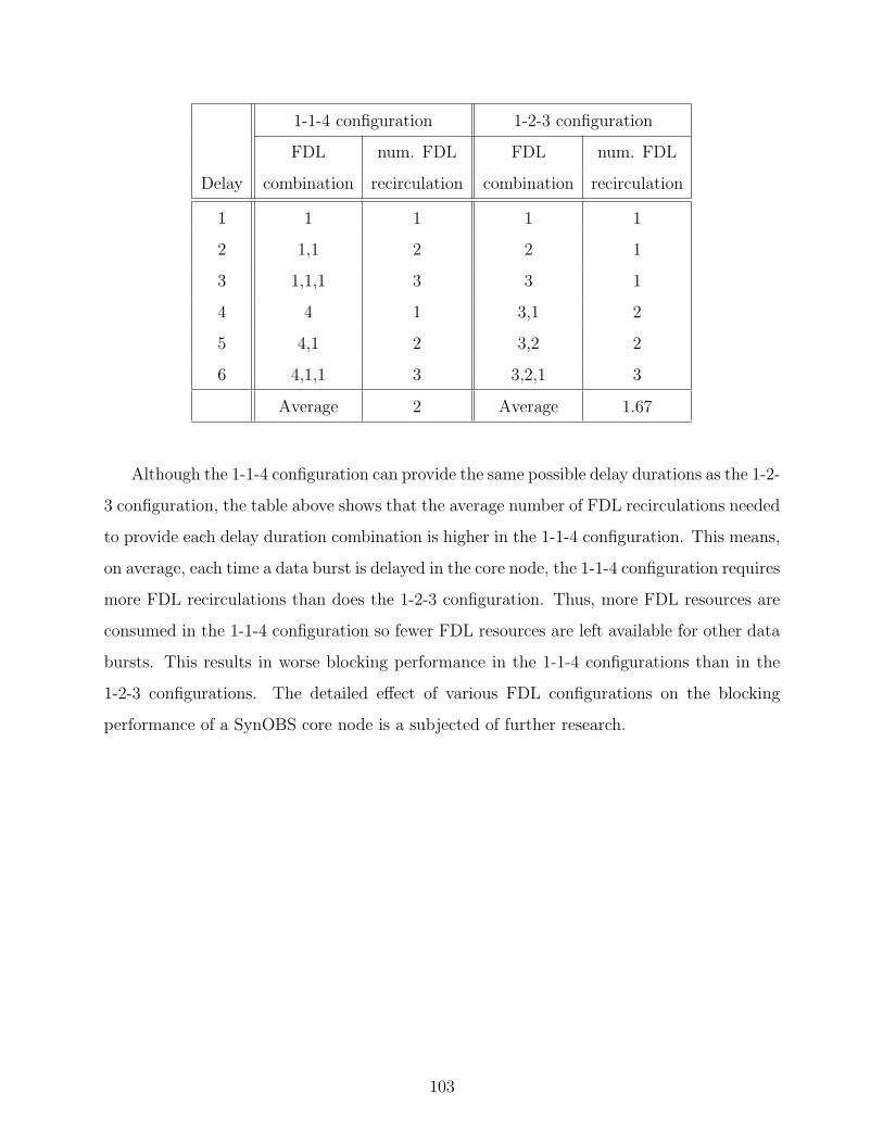
1-1-4 configuration 1-2-3 configuration
FDL num. FDL FDL num. FDL
Delay combination recirculation combination recirculation
1 1 1 1 1
2 1,1 2 2 1
3 1,1,1 3 3 1
4 4 1 3,1 2
5 4,1 2 3,2 2
6 4,1,1 3 3,2,1 3
Average 2 Average 1.67
Although the 1-1-4 configuration can provide the same possible delay durations as the 1-2-
3 configuration, the table above shows that the average number of FDL recirculations needed
to provide each delay duration combination is higher in the 1-1-4 configuration. This means,
on average, each time a data burst is delayed in the core node, the 1-1-4 configuration requires
more FDL recirculations than does the 1-2-3 configuration. Thus, more FDL resources are
consumed in the 1-1-4 configuration so fewer FDL resources are left available for other data
bursts. This results in worse blocking performance in the 1-1-4 configurations than in the
1-2-3 configurations. The detailed effect of various FDL configurations on the blocking
performance of a SynOBS core node is a subjected of further research.
103
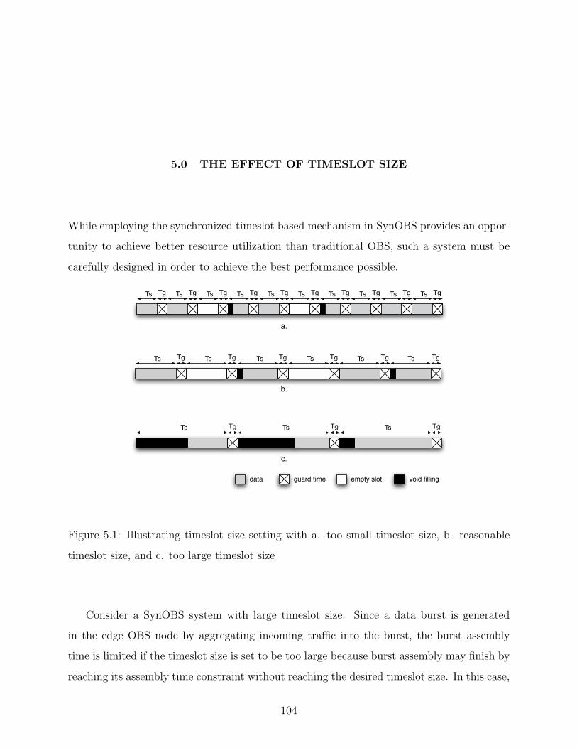
5.0 THE EFFECT OF TIMESLOT SIZE
While employing the synchronized timeslot based mechanism in SynOBS provides an oppor-
tunity to achieve better resource utilization than traditional OBS, such a system must be
carefully designed in order to achieve the best performance possible.
TgTgTgTgTgTs Tg Ts Ts Ts Ts Ts
a.
TgTgTg Ts TsTs
b.
guard timedata empty slot void filling
Ts Tg Ts Tg Ts Tg Ts Tg Ts Tg Ts Tg Ts Tg Ts Tg Ts Tg Ts Tg
c.
Figure 5.1: Illustrating timeslot size setting with a. too small timeslot size, b. reasonable
timeslot size, and c. too large timeslot size
Consider a SynOBS system with large timeslot size. Since a data burst is generated
in the edge OBS node by aggregating incoming traffic into the burst, the burst assembly
time is limited if the timeslot size is set to be too large because burst assembly may finish by
reaching its assembly time constraint without reaching the desired timeslot size. In this case,
104
many of the data bursts are partially filled in their timeslots, and thus, resource utilization
is wasted. This wasted resource, caused by under-utilized burst assembly algorithm in the
edge SynOBS nodes, causes an unnecessarily large percentage of data bursts to be reserved,
which results in higher blocking probabilities in the core SynOBS nodes.
Now consider a SynOBS system with small timeslot size. In this case, most of the
assembled data bursts reach the desired timeslot size before their assembly time constraint
expires, and most of the timeslots are filled. However, resource utilization is compromised by
the guard time between the timeslots because the smaller the timeslot size, the more often
the guard time occurs in the data channel. Since data cannot be transmitted during the
guard time, this results in a loss of resource utilization and available bandwidth for the data
traffic, which subsequently causes the burst blocking probabilities to be increased. Figure
5.1 illustrates examples with a small timeslot setting, a reasonable timeslot setting, and a
large timeslot setting.
The effect of timeslot size setting results from the trade-off between the burst assembly
time constraint and the duration of guard time between each consecutive timeslot. This
happens because the SynOBS is based on a fixed-size timeslot mechanism. This disserta-
tion investigates the effect on timeslot size setting on the performance of SynOBS in order
to provide an analytical framework for estimating the optimized solution, based on given
network configuration and input traffic characteristic, which has been presented in [42].
5.1 SYNOBS BURST ASSEMBLY ALGORITHM
In SynOBS, since each data burst is fit into a timeslot before being sent out to the outgoing
data wavelength, each data bursts size is limited by the duration of the timeslot. Because
the burst assembly algorithm for SynOBS has to assemble incoming data packets into a
burst with length less than or equal to the timeslot duration, a simple modified version of
the Max-Time-Max-Length [2] burst assembly algorithm is used as the model for the burst
assembly algorithm in SynOBS. The algorithm uses the maximum assembly time (T ) and
the target burst size (L) as its criteria for assembling a data burst. It works by assembling
105
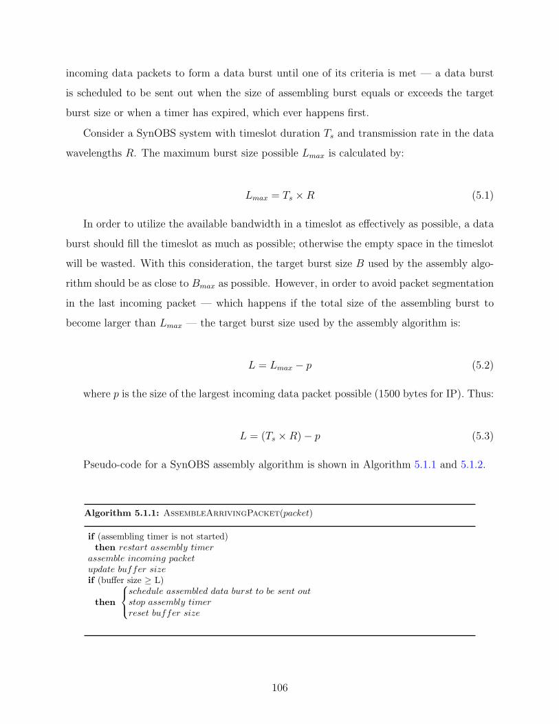
incoming data packets to form a data burst until one of its criteria is met — a data burst
is scheduled to be sent out when the size of assembling burst equals or exceeds the target
burst size or when a timer has expired, which ever happens first.
Consider a SynOBS system with timeslot duration Ts and transmission rate in the data
wavelengths R. The maximum burst size possible Lmax is calculated by:
Lmax = Ts ×R (5.1)
In order to utilize the available bandwidth in a timeslot as effectively as possible, a data
burst should fill the timeslot as much as possible; otherwise the empty space in the timeslot
will be wasted. With this consideration, the target burst size B used by the assembly algo-
rithm should be as close to Bmax as possible. However, in order to avoid packet segmentation
in the last incoming packet — which happens if the total size of the assembling burst to
become larger than Lmax — the target burst size used by the assembly algorithm is:
L = Lmax − p (5.2)
where p is the size of the largest incoming data packet possible (1500 bytes for IP). Thus:
L = (Ts ×R)− p (5.3)
Pseudo-code for a SynOBS assembly algorithm is shown in Algorithm 5.1.1 and 5.1.2.
Algorithm 5.1.1: AssembleArrivingPacket(packet)
if (assembling timer is not started)then restart assembly timer
assemble incoming packetupdate buffer sizeif (buffer size ≥ L)
then
schedule assembled data burst to be sent outstop assembly timerreset buffer size
106
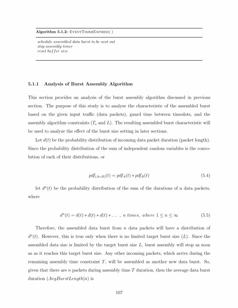
Algorithm 5.1.2: EventTimerExpired( )
schedule assembled data burst to be sent outstop assembly timerreset buffer size
5.1.1 Analysis of Burst Assembly Algorithm
This section provides an analysis of the burst assembly algorithm discussed in previous
section. The purpose of this study is to analyze the characteristic of the assembled burst
based on the given input traffic (data packets), guard time between timeslots, and the
assembly algorithm constraints (Ts and L). The resulting assembled burst characteristic will
be used to analyze the effect of the burst size setting in later sections.
Let d(t) be the probability distribution of incoming data packet duration (packet length).
Since the probability distribution of the sum of independent random variables is the convo-
lution of each of their distributions, or
pdf(A+B)(t) = pdfA(t) ∗ pdfB(t) (5.4)
let dn(t) be the probability distribution of the sum of the durations of n data packets,
where
dn(t) = d(t) ∗ d(t) ∗ d(t) ∗ . . . , n times, where 1 ≤ n ≤ ∞ (5.5)
Therefore, the assembled data burst from n data packets will have a distribution of
dn(t). However, this is true only when there is no limited target burst size (L). Since the
assembled data size is limited by the target burst size L, burst assembly will stop as soon
as as it reaches this target burst size. Any other incoming packets, which arrive during the
remaining assembly time constraint T , will be assembled as another new data burst. So,
given that there are n packets during assembly time T duration, then the average data burst
duration (AvgBurstLength|n) is
107
AvgBurstLength|n =
∫ L
0
t · dn(t) dt+ (L+ φn)
∫ ∞L
dn(t) dt
=
∫ L
0
t · dn(t) dt+ (L+ φn)(1−
∫ L
0
dn(t) dt)
(5.6)
where φn is an average length of assembled data burst portion that exceeds the target
timeslot size L, given that n packets arrive during assembly time T , or
φn =
∑ni=1
[ ∫ L0
(di−1(l) ·
∫∞L−l
(d1(x) · (x+ l − L)
)dx
)dl
]1−
∫ L0dn(t) dt
(5.7)
If the probability that there are n arrivals during an assembly time constraint duration
T is P(n) then, the average assembled data burst length is calculated by following equation.
AvgBurstLength =∞∑n=0
{P (n)
[AvgBurstLength|(n+ 1)
]}=
∞∑n=0
{P (n)
[ ∫ L
0
t · dn+1(t) dt+ (L+ φn+1)
∫ ∞L
dn+1(t) dt
]}=
∞∑n=0
{P (n)
[ ∫ L
0
t · dn+1(t) dt+ (L+ φn+1)(1−
∫ L
0
dn+1(t) dt)]}(5.8)
Notice that AvgBurstLength|(n + 1) is used instead of AvgBurstLength|n. This is
because there is one packet at burst assembling start time, and there are n arrivals during
time constraint T .
Assuming that packet arrival is Poisson distributed with rate λ and that packet duration
is exponentially distributed with average length l = 1/µ, then
P (n) =e−λT (λT )n
n!(5.9)
108
By the memoryless property of the exponential distribution, the average length of the
assembled data burst portion that exceeds the target timeslot size, given that n packets
arrive during assembly time T , is φn = 1/µ [37].
Since the Erlang distribution is the distribution of the sum of n independent identi-
cally distributed random variables each having an exponential distribution [37], equation 5.5
becomes:
dn(t) =µnt(n−1)e−µt
(n− 1)!(5.10)
and,
∫ ∞L
dn(t) dt = e−µL( n−1∑
i=0
(µL)i
i!
)(5.11)
From equation 5.8, the average assembled data burst length can be calculated by
AvgBurstLength =∞∑n=0
{e−λT (λT )n
n!
[ ∫ L
0
(µn+1tn+1e−µt
n!
)dt+ (L+
1
µ) · e−µL(
n∑i=0
(µL)i
i!)
]}=
∞∑n=0
{e−λT (λT )n
n!
[µn+1
n!
∫ L
0
(tn+1e−µt) dt+ (L+1
µ) · e−µL(
n∑i=0
(µL)i
i!)
]}(5.12)
Figure 5.2 illustrates the average assembled data length that is generated by the assem-
bly algorithm with respect to the incoming packet arrival rate. The graph results from a
calculation with an average data packet length of 0.8 µsec and 1 msec burst assembly time
constraint. Several timeslot size settings are shown in the graph, including 10, 30, 50, 70,
and 90 µsec. In every timeslot size setting, the figure shows that, as the packet arrival
rate increases, the average assembled data length increases as well. At a low packet arrival
rate, the average assembled data lengths are the same among different timeslot size settings,
and increase almost linearly according to the given arrival rate. However, at the higher
packet arrival rate, the average assembled data length begins to saturate. This is caused by
the timeslot size limit, where the smaller timeslot size setting begins to saturate first, and
109
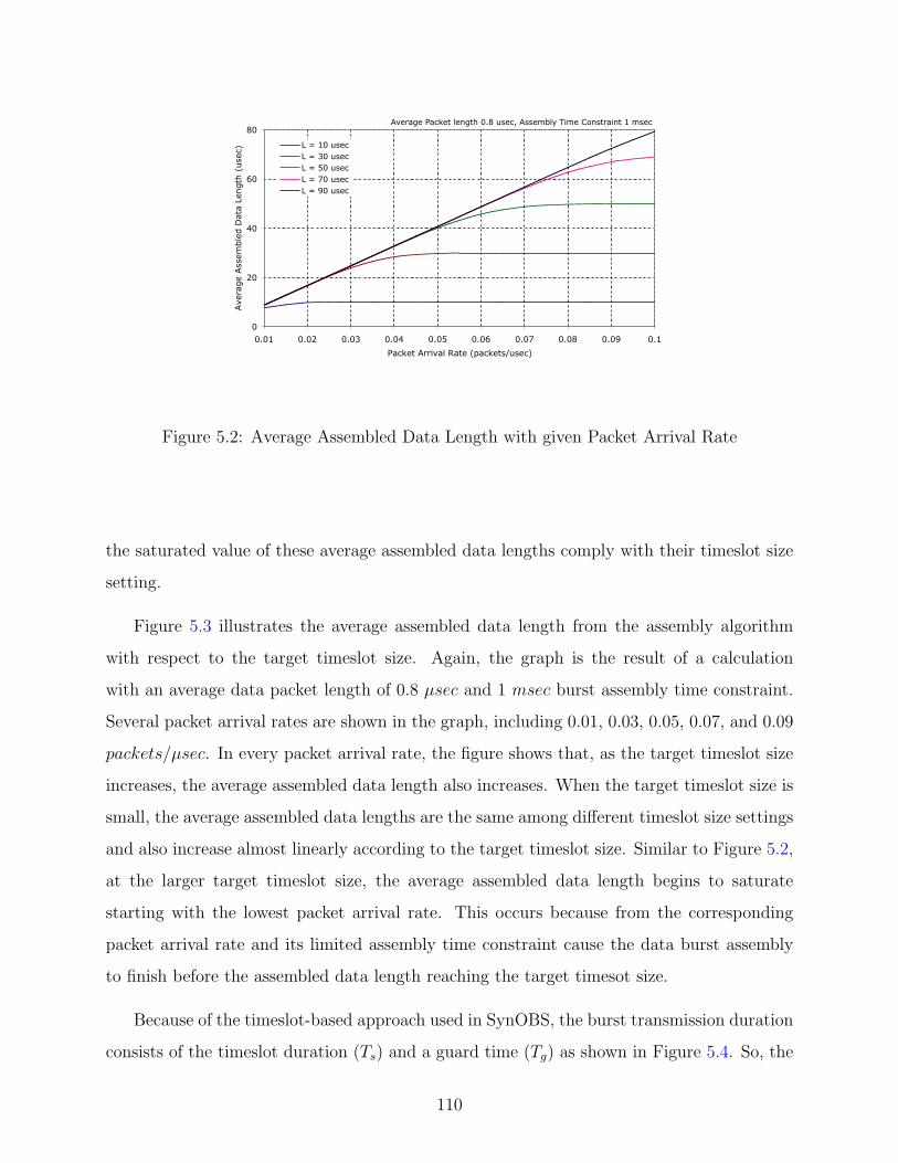
0
20
40
60
80
0.01 0.02 0.03 0.04 0.05 0.06 0.07 0.08 0.09 0.1
Packet Arrival Rate (packets/usec)
Ave
rage
Ass
emble
d D
ata
Length
(use
c)
L = 10 usecL = 30 usecL = 50 usecL = 70 usecL = 90 usec
Average Packet length 0.8 usec, Assembly Time Constraint 1 msec
Figure 5.2: Average Assembled Data Length with given Packet Arrival Rate
the saturated value of these average assembled data lengths comply with their timeslot size
setting.
Figure 5.3 illustrates the average assembled data length from the assembly algorithm
with respect to the target timeslot size. Again, the graph is the result of a calculation
with an average data packet length of 0.8 µsec and 1 msec burst assembly time constraint.
Several packet arrival rates are shown in the graph, including 0.01, 0.03, 0.05, 0.07, and 0.09
packets/µsec. In every packet arrival rate, the figure shows that, as the target timeslot size
increases, the average assembled data length also increases. When the target timeslot size is
small, the average assembled data lengths are the same among different timeslot size settings
and also increase almost linearly according to the target timeslot size. Similar to Figure 5.2,
at the larger target timeslot size, the average assembled data length begins to saturate
starting with the lowest packet arrival rate. This occurs because from the corresponding
packet arrival rate and its limited assembly time constraint cause the data burst assembly
to finish before the assembled data length reaching the target timesot size.
Because of the timeslot-based approach used in SynOBS, the burst transmission duration
consists of the timeslot duration (Ts) and a guard time (Tg) as shown in Figure 5.4. So, the
110
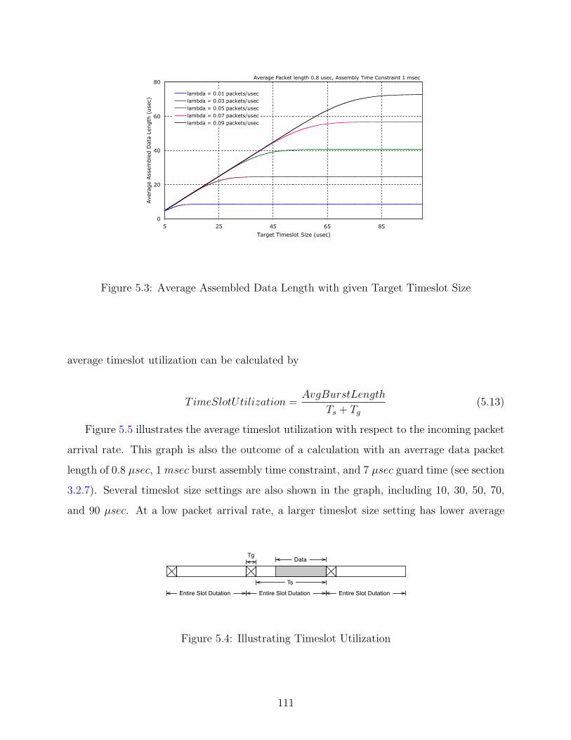
0
20
40
60
80
5 25 45 65 85
Target Timeslot Size (usec)
Ave
rage
Ass
emble
d D
ata
Length
(use
c)
lambda = 0.01 packets/useclambda = 0.03 packets/useclambda = 0.05 packets/useclambda = 0.07 packets/useclambda = 0.09 packets/usec
Average Packet length 0.8 usec, Assembly Time Constraint 1 msec
Figure 5.3: Average Assembled Data Length with given Target Timeslot Size
average timeslot utilization can be calculated by
TimeSlotUtilization =AvgBurstLength
Ts + Tg(5.13)
Figure 5.5 illustrates the average timeslot utilization with respect to the incoming packet
arrival rate. This graph is also the outcome of a calculation with an averrage data packet
length of 0.8 µsec, 1 msec burst assembly time constraint, and 7 µsec guard time (see section
3.2.7). Several timeslot size settings are also shown in the graph, including 10, 30, 50, 70,
and 90 µsec. At a low packet arrival rate, a larger timeslot size setting has lower average
Ts
DataTg
Entire Slot Dutation Entire Slot DutationEntire Slot Dutation
Figure 5.4: Illustrating Timeslot Utilization
111
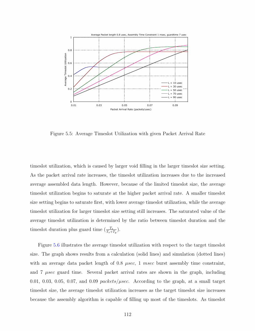
0
0.2
0.4
0.6
0.8
1
0.01 0.03 0.05 0.07 0.09
Packet Arrival Rate (packets/usec)
Ave
rage
Tim
eslo
t U
tiliz
atio
n
L = 10 usec
L = 30 usec
L = 50 usec
L = 70 usec
L = 90 usec
Average Packet length 0.8 usec, Assembly Time Constraint 1 msec, guardtime 7 usec
Figure 5.5: Average Timeslot Utilization with given Packet Arrival Rate
timeslot utilization, which is caused by larger void filling in the larger timeslot size setting.
As the packet arrival rate increases, the timeslot utilization increases due to the increased
average assembled data length. However, because of the limited timeslot size, the average
timeslot utilization begins to saturate at the higher packet arrival rate. A smaller timeslot
size setting begins to saturate first, with lower average timeslot utilization, while the average
timeslot utilization for larger timeslot size setting still increases. The saturated value of the
average timeslot utilization is determined by the ratio between timeslot duration and the
timeslot duration plus guard time ( TsTs+Tg
).
Figure 5.6 illustrates the average timeslot utilization with respect to the target timeslot
size. The graph shows results from a calculation (solid lines) and simulation (dotted lines)
with an average data packet length of 0.8 µsec, 1 msec burst assembly time constraint,
and 7 µsec guard time. Several packet arrival rates are shown in the graph, including
0.01, 0.03, 0.05, 0.07, and 0.09 packets/µsec. According to the graph, at a small target
timeslot size, the average timeslot utilization increases as the target timeslot size increases
because the assembly algorithm is capable of filling up most of the timeslots. As timeslot
112
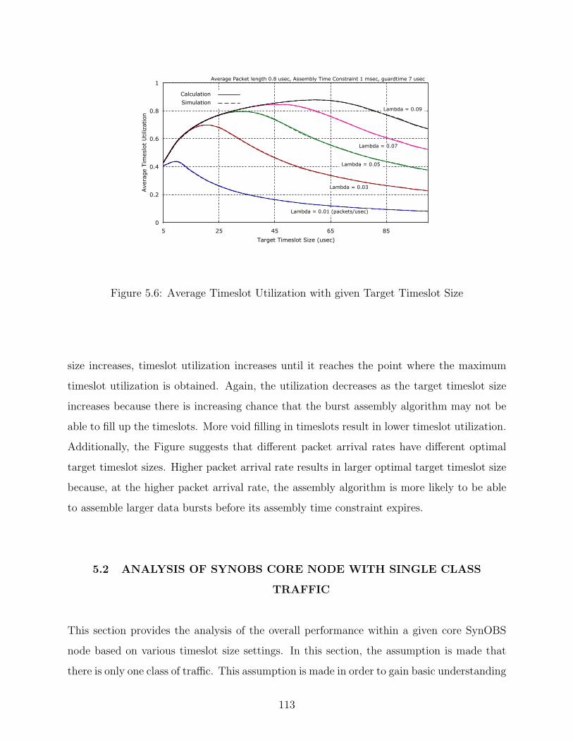
0
0.2
0.4
0.6
0.8
1
5 25 45 65 85
Target Timeslot Size (usec)
Ave
rage
Tim
eslo
t U
tiliz
atio
n
Calculation
Simulation
Lambda = 0.01 (packets/usec)
Lambda = 0.09
Lambda = 0.03
Lambda = 0.05
Lambda = 0.07
Average Packet length 0.8 usec, Assembly Time Constraint 1 msec, guardtime 7 usec
Figure 5.6: Average Timeslot Utilization with given Target Timeslot Size
size increases, timeslot utilization increases until it reaches the point where the maximum
timeslot utilization is obtained. Again, the utilization decreases as the target timeslot size
increases because there is increasing chance that the burst assembly algorithm may not be
able to fill up the timeslots. More void filling in timeslots result in lower timeslot utilization.
Additionally, the Figure suggests that different packet arrival rates have different optimal
target timeslot sizes. Higher packet arrival rate results in larger optimal target timeslot size
because, at the higher packet arrival rate, the assembly algorithm is more likely to be able
to assemble larger data bursts before its assembly time constraint expires.
5.2 ANALYSIS OF SYNOBS CORE NODE WITH SINGLE CLASS
TRAFFIC
This section provides the analysis of the overall performance within a given core SynOBS
node based on various timeslot size settings. In this section, the assumption is made that
there is only one class of traffic. This assumption is made in order to gain basic understanding
113
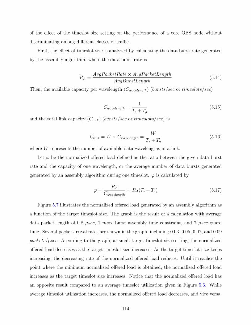
of the effect of the timeslot size setting on the performance of a core OBS node without
discriminating among different classes of traffic.
First, the effect of timeslot size is analyzed by calculating the data burst rate generated
by the assembly algorithm, where the data burst rate is
RA =AvgPacketRate× AvgPacketLength
AvgBurstLength(5.14)
Then, the available capacity per wavelength (Cwavelength) (bursts/sec or timeslots/sec)
Cwavelength =1
Ts + Tg(5.15)
and the total link capacity (Clink) (bursts/sec or timeslots/sec) is
Clink = W × Cwavelength =W
Ts + Tg(5.16)
where W represents the number of available data wavelengths in a link.
Let ϕ be the normalized offered load defined as the ratio between the given data burst
rate and the capacity of one wavelength, or the average number of data bursts generated
generated by an assembly algorithm during one timeslot. ϕ is calculated by
ϕ =RA
Cwavelength= RA(Ts + Tg) (5.17)
Figure 5.7 illustrates the normalized offered load generated by an assembly algorithm as
a function of the target timeslot size. The graph is the result of a calculation with average
data packet length of 0.8 µsec, 1 msec burst assembly time constraint, and 7 µsec guard
time. Several packet arrival rates are shown in the graph, including 0.03, 0.05, 0.07, and 0.09
packets/µsec. According to the graph, at small target timeslot size setting, the normalized
offered load decreases as the target timeslot size increases. As the target timeslot size keeps
increasing, the decreasing rate of the normalized offered load reduces. Until it reaches the
point where the minimum normalized offered load is obtained, the normalized offered load
increases as the target timeslot size increases. Notice that the normalized offered load has
an opposite result compared to an average timeslot utilization given in Figure 5.6. While
average timeslot utilization increases, the normalized offered load decreases, and vice versa.
114
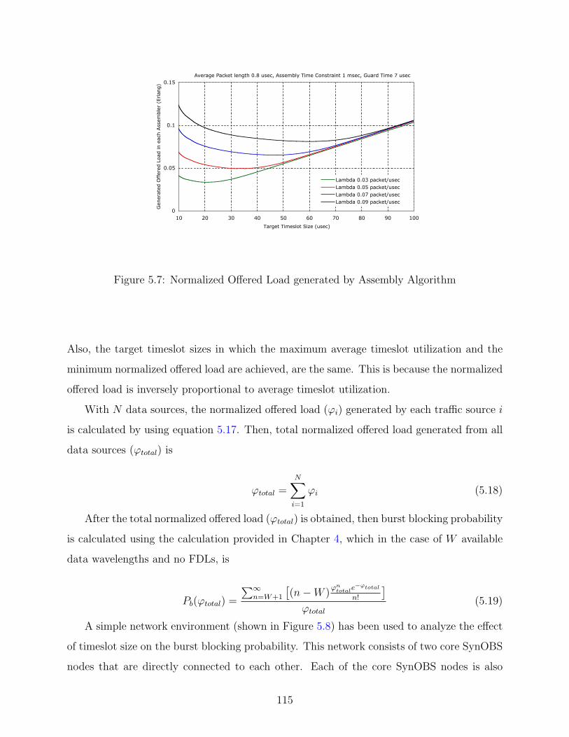
0
0.05
0.1
0.15
10 20 30 40 50 60 70 80 90 100
Target Timeslot Size (usec)
Gen
erat
ed O
ffer
ed L
oad
in e
ach A
ssem
ble
r (E
rlan
g)
Lambda 0.03 packet/usecLambda 0.05 packet/usecLambda 0.07 packet/usecLambda 0.09 packet/usec
Average Packet length 0.8 usec, Assembly Time Constraint 1 msec, Guard Time 7 usec
Figure 5.7: Normalized Offered Load generated by Assembly Algorithm
Also, the target timeslot sizes in which the maximum average timeslot utilization and the
minimum normalized offered load are achieved, are the same. This is because the normalized
offered load is inversely proportional to average timeslot utilization.
With N data sources, the normalized offered load (ϕi) generated by each traffic source i
is calculated by using equation 5.17. Then, total normalized offered load generated from all
data sources (ϕtotal) is
ϕtotal =N∑i=1
ϕi (5.18)
After the total normalized offered load (ϕtotal) is obtained, then burst blocking probability
is calculated using the calculation provided in Chapter 4, which in the case of W available
data wavelengths and no FDLs, is
Pb(ϕtotal) =
∑∞n=W+1
[(n−W )
ϕntotale−ϕtotal
n!
]ϕtotal
(5.19)
A simple network environment (shown in Figure 5.8) has been used to analyze the effect
of timeslot size on the burst blocking probability. This network consists of two core SynOBS
nodes that are directly connected to each other. Each of the core SynOBS nodes is also
115
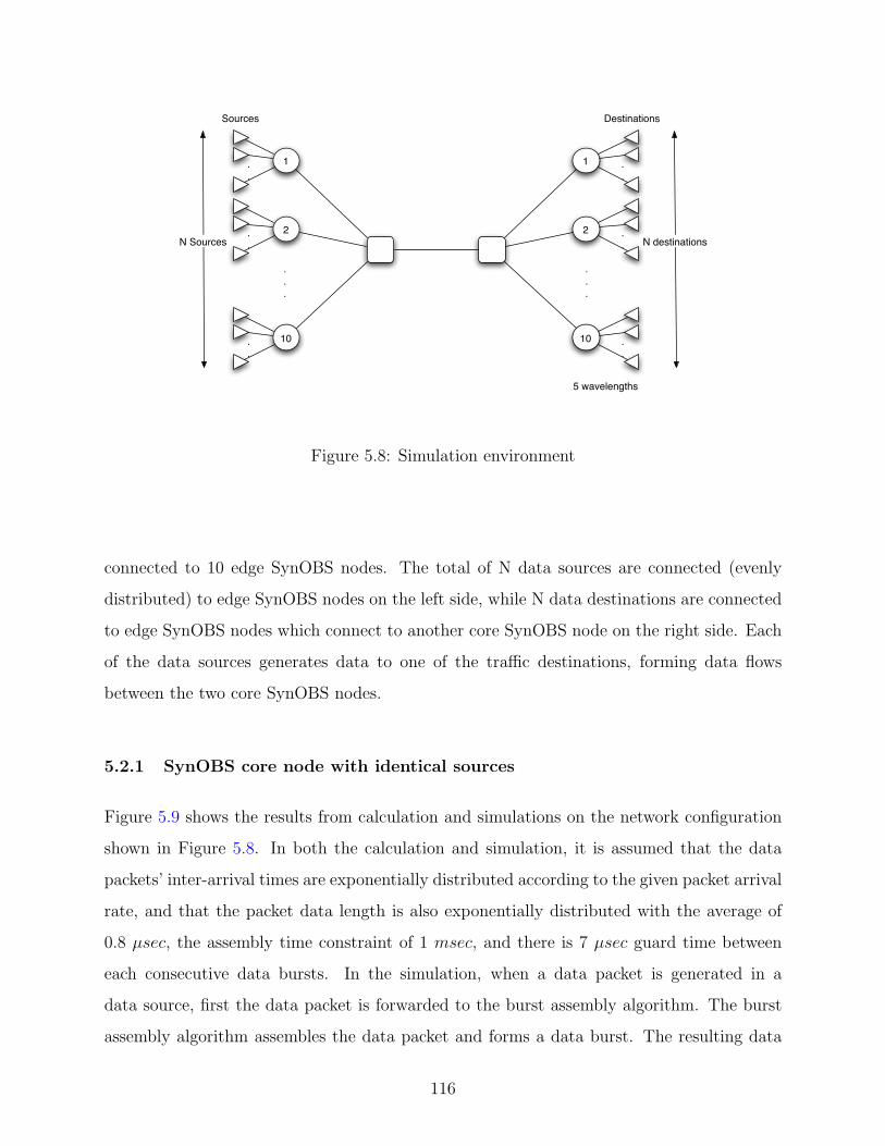
1..
2..
10..
.
.
.
1 ..
2 ..
10 ..
.
.
.
5 wavelengths
N destinationsN Sources
Sources Destinations
Figure 5.8: Simulation environment
connected to 10 edge SynOBS nodes. The total of N data sources are connected (evenly
distributed) to edge SynOBS nodes on the left side, while N data destinations are connected
to edge SynOBS nodes which connect to another core SynOBS node on the right side. Each
of the data sources generates data to one of the traffic destinations, forming data flows
between the two core SynOBS nodes.
5.2.1 SynOBS core node with identical sources
Figure 5.9 shows the results from calculation and simulations on the network configuration
shown in Figure 5.8. In both the calculation and simulation, it is assumed that the data
packets’ inter-arrival times are exponentially distributed according to the given packet arrival
rate, and that the packet data length is also exponentially distributed with the average of
0.8 µsec, the assembly time constraint of 1 msec, and there is 7 µsec guard time between
each consecutive data bursts. In the simulation, when a data packet is generated in a
data source, first the data packet is forwarded to the burst assembly algorithm. The burst
assembly algorithm assembles the data packet and forms a data burst. The resulting data
116
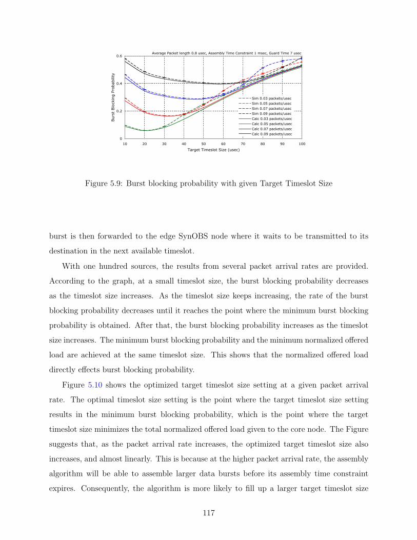
0
0.2
0.4
0.6
10 20 30 40 50 60 70 80 90 100
Target Timeslot Size (usec)
Burs
t Blo
ckin
g P
robab
ility
Sim 0.03 packets/usecSim 0.05 packets/usecSim 0.07 packets/usecSim 0.09 packets/usecCalc 0.03 packets/usecCalc 0.05 packets/usecCalc 0.07 packets/usecCalc 0.09 packets/usec
Average Packet length 0.8 usec, Assembly Time Constraint 1 msec, Guard Time 7 usec
Figure 5.9: Burst blocking probability with given Target Timeslot Size
burst is then forwarded to the edge SynOBS node where it waits to be transmitted to its
destination in the next available timeslot.
With one hundred sources, the results from several packet arrival rates are provided.
According to the graph, at a small timeslot size, the burst blocking probability decreases
as the timeslot size increases. As the timeslot size keeps increasing, the rate of the burst
blocking probability decreases until it reaches the point where the minimum burst blocking
probability is obtained. After that, the burst blocking probability increases as the timeslot
size increases. The minimum burst blocking probability and the minimum normalized offered
load are achieved at the same timeslot size. This shows that the normalized offered load
directly effects burst blocking probability.
Figure 5.10 shows the optimized target timeslot size setting at a given packet arrival
rate. The optimal timeslot size setting is the point where the target timeslot size setting
results in the minimum burst blocking probability, which is the point where the target
timeslot size minimizes the total normalized offered load given to the core node. The Figure
suggests that, as the packet arrival rate increases, the optimized target timeslot size also
increases, and almost linearly. This is because at the higher packet arrival rate, the assembly
algorithm will be able to assemble larger data bursts before its assembly time constraint
expires. Consequently, the algorithm is more likely to fill up a larger target timeslot size
117
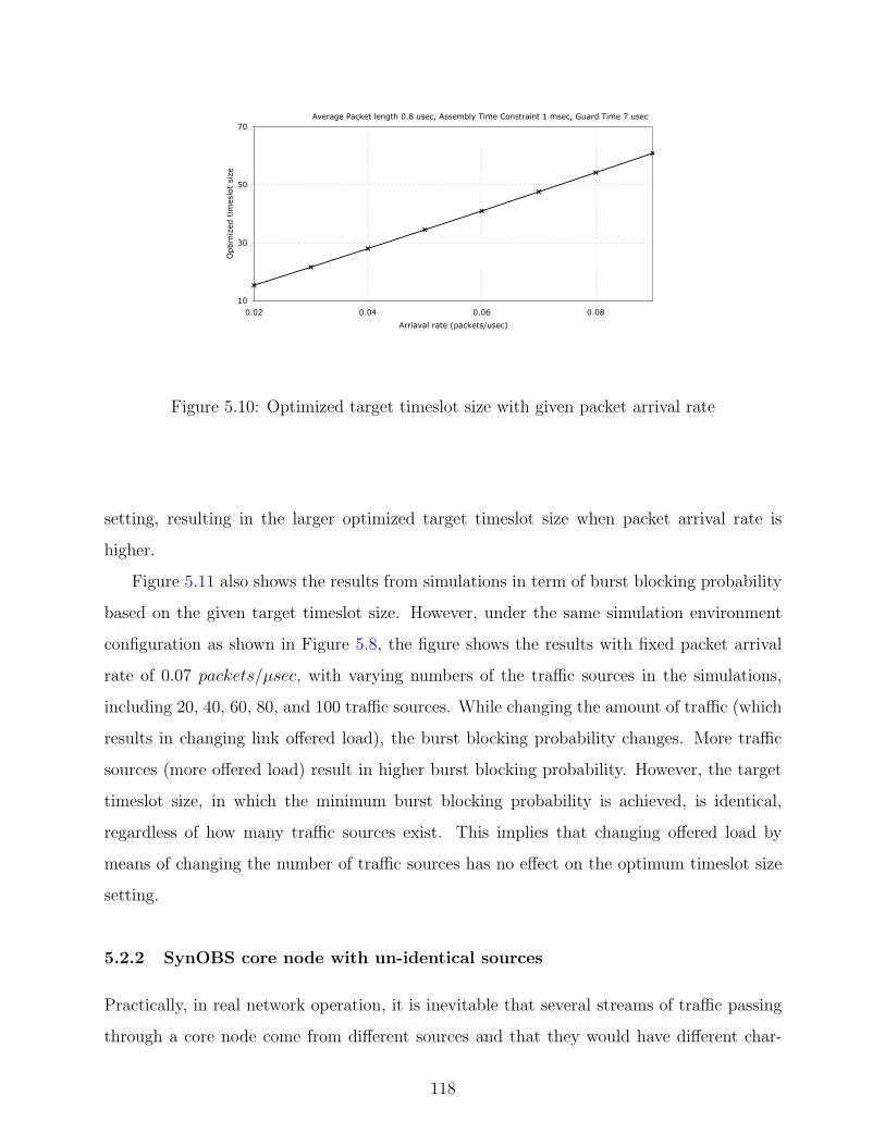
10
30
50
70
0.02 0.04 0.06 0.08
Arriaval rate (packets/usec)
Optim
ized
tim
eslo
t si
ze
Average Packet length 0.8 usec, Assembly Time Constraint 1 msec, Guard Time 7 usec
Figure 5.10: Optimized target timeslot size with given packet arrival rate
setting, resulting in the larger optimized target timeslot size when packet arrival rate is
higher.
Figure 5.11 also shows the results from simulations in term of burst blocking probability
based on the given target timeslot size. However, under the same simulation environment
configuration as shown in Figure 5.8, the figure shows the results with fixed packet arrival
rate of 0.07 packets/µsec, with varying numbers of the traffic sources in the simulations,
including 20, 40, 60, 80, and 100 traffic sources. While changing the amount of traffic (which
results in changing link offered load), the burst blocking probability changes. More traffic
sources (more offered load) result in higher burst blocking probability. However, the target
timeslot size, in which the minimum burst blocking probability is achieved, is identical,
regardless of how many traffic sources exist. This implies that changing offered load by
means of changing the number of traffic sources has no effect on the optimum timeslot size
setting.
5.2.2 SynOBS core node with un-identical sources
Practically, in real network operation, it is inevitable that several streams of traffic passing
through a core node come from different sources and that they would have different char-
118
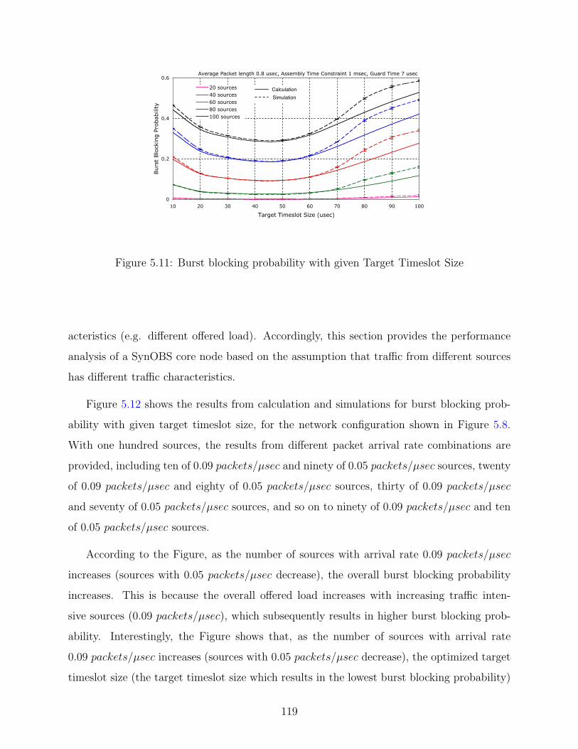
0
0.2
0.4
0.6
10 20 30 40 50 60 70 80 90 100
Target Timeslot Size (usec)
Burs
t Blo
ckin
g P
robab
ility
Average Packet length 0.8 usec, Assembly Time Constraint 1 msec, Guard Time 7 usec
0
0.2
0.4
0.6
10 20 30 40 50 60 70 80 90 100
Target Timeslot Size (usec)
Burs
t Blo
ckin
g P
robability
20 sources
40 sources
60 sources
80 sources
100 sources
Average Packet length 0.8 usec, Assembly Time Constraint 1 msec, Guard Time 7 usec
CalculationSimulation
Figure 5.11: Burst blocking probability with given Target Timeslot Size
acteristics (e.g. different offered load). Accordingly, this section provides the performance
analysis of a SynOBS core node based on the assumption that traffic from different sources
has different traffic characteristics.
Figure 5.12 shows the results from calculation and simulations for burst blocking prob-
ability with given target timeslot size, for the network configuration shown in Figure 5.8.
With one hundred sources, the results from different packet arrival rate combinations are
provided, including ten of 0.09 packets/µsec and ninety of 0.05 packets/µsec sources, twenty
of 0.09 packets/µsec and eighty of 0.05 packets/µsec sources, thirty of 0.09 packets/µsec
and seventy of 0.05 packets/µsec sources, and so on to ninety of 0.09 packets/µsec and ten
of 0.05 packets/µsec sources.
According to the Figure, as the number of sources with arrival rate 0.09 packets/µsec
increases (sources with 0.05 packets/µsec decrease), the overall burst blocking probability
increases. This is because the overall offered load increases with increasing traffic inten-
sive sources (0.09 packets/µsec), which subsequently results in higher burst blocking prob-
ability. Interestingly, the Figure shows that, as the number of sources with arrival rate
0.09 packets/µsec increases (sources with 0.05 packets/µsec decrease), the optimized target
timeslot size (the target timeslot size which results in the lowest burst blocking probability)
119
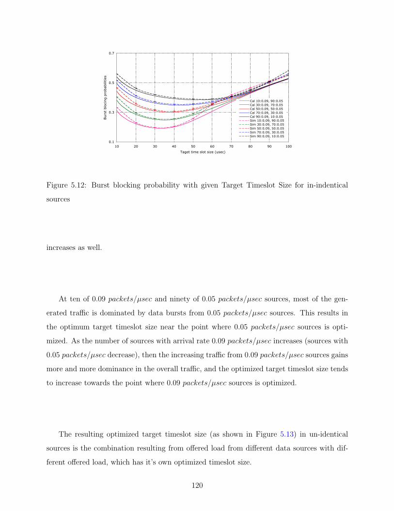
0.1
0.3
0.5
0.7
10 20 30 40 50 60 70 80 90 100
Taget time slot size (usec)
Burs
t blo
cing p
robab
ilities
Cal 10:0.09, 90:0.05Cal 30:0.09, 70:0.05Cal 50:0.09, 50:0.05Cal 70:0.09, 30:0.05Cal 90:0.09, 10:0.05Sim 10:0.09, 90:0.05Sim 30:0.09, 70:0.05Sim 50:0.09, 50:0.05Sim 70:0.09, 30:0.05Sim 90:0.09, 10:0.05
Figure 5.12: Burst blocking probability with given Target Timeslot Size for in-indentical
sources
increases as well.
At ten of 0.09 packets/µsec and ninety of 0.05 packets/µsec sources, most of the gen-
erated traffic is dominated by data bursts from 0.05 packets/µsec sources. This results in
the optimum target timeslot size near the point where 0.05 packets/µsec sources is opti-
mized. As the number of sources with arrival rate 0.09 packets/µsec increases (sources with
0.05 packets/µsec decrease), then the increasing traffic from 0.09 packets/µsec sources gains
more and more dominance in the overall traffic, and the optimized target timeslot size tends
to increase towards the point where 0.09 packets/µsec sources is optimized.
The resulting optimized target timeslot size (as shown in Figure 5.13) in un-identical
sources is the combination resulting from offered load from different data sources with dif-
ferent offered load, which has it’s own optimized timeslot size.
120
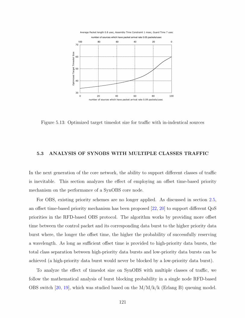
30
40
50
60
70
0 20 40 60 80 100
number of sources which have packet arrival rate 0.09 packets/usec
Optim
ized
Tar
get
Tim
eslo
t Siz
e
number of sources which have packet arrival rate 0.05 packets/usec
020406080100
Average Packet length 0.8 usec, Assembly Time Constraint 1 msec, Guard Time 7 usec
Figure 5.13: Optimized target timeslot size for traffic with in-indentical sources
5.3 ANALYSIS OF SYNOBS WITH MULTIPLE CLASSES TRAFFIC
In the next generation of the core network, the ability to support different classes of traffic
is inevitable. This section analyzes the effect of employing an offset time-based priority
mechanism on the performance of a SynOBS core node.
For OBS, existing priority schemes are no longer applied. As discussed in section 2.5,
an offset time-based priority mechanism has been proposed [22, 20] to support different QoS
priorities in the RFD-based OBS protocol. The algorithm works by providing more offset
time between the control packet and its corresponding data burst to the higher priority data
burst where, the longer the offset time, the higher the probability of successfully reserving
a wavelength. As long as sufficient offset time is provided to high-priority data bursts, the
total class separation between high-priority data bursts and low-priority data bursts can be
achieved (a high-priority data burst would never be blocked by a low-priority data burst).
To analyze the effect of timeslot size on SynOBS with multiple classes of traffic, we
follow the mathematical analysis of burst blocking probability in a single node RFD-based
OBS switch [20, 19], which was studied based on the M/M/k/k (Erlang B) queuing model.
121
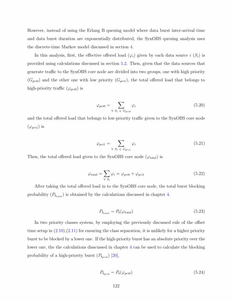
However, instead of using the Erlang B queuing model where data burst inter-arrival time
and data burst duration are exponentially distributed, the SynOBS queuing analysis uses
the discrete-time Markov model discussed in section 4.
In this analysis, first, the effective offered load (ϕi) given by each data source i (Si) is
provided using calculations discussed in section 5.2. Then, given that the data sources that
generate traffic to the SynOBS core node are divided into two groups, one with high priority
(Gpri0) and the other one with low priority (Gpri1), the total offered load that belongs to
high-priority traffic (ϕpri0) is
ϕpri0 =∑
∀ Si ∈ Gpri0
ϕi (5.20)
and the total offered load that belongs to low-priority traffic given to the SynOBS core node
(ϕpri1) is
ϕpri1 =∑
∀ Si ∈ Gpri1
ϕi (5.21)
Then, the total offered load given to the SynOBS core node (ϕtotal) is
ϕtotal =∑∀ Si
ϕi = ϕpri0 + ϕpri1 (5.22)
After taking the total offered load in to the SynOBS core node, the total burst blocking
probability (Pbtotal) is obtained by the calculations discussed in chapter 4.
Pbtotal = Pb(ϕtotal) (5.23)
In two priority classes system, by employing the previously discussed rule of the offset
time setup in (2.10),(2.11) for ensuring the class separation, it is unlikely for a higher priority
burst to be blocked by a lower one. If the high-priority burst has an absolute priority over the
lower one, the the calculations disscussed in chapter 4 can be used to calculate the blocking
probability of a high-priority burst (Pbpri0) [20],
Pbpri0 = Pb(ϕpri0) (5.24)
122
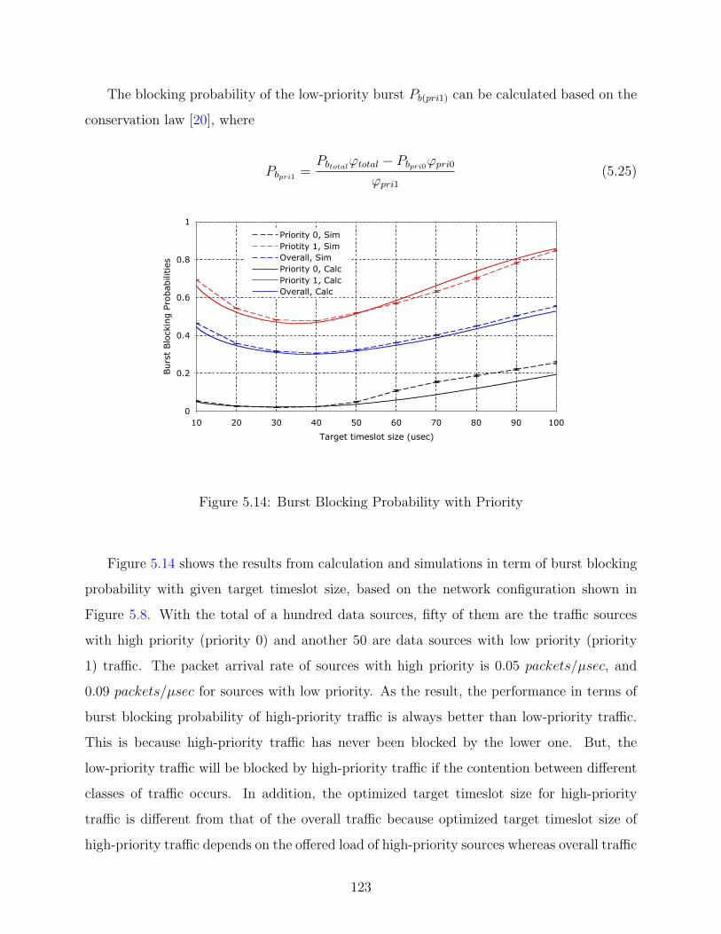
The blocking probability of the low-priority burst Pb(pri1) can be calculated based on the
conservation law [20], where
Pbpri1 =Pbtotalϕtotal − Pbpri0ϕpri0
ϕpri1(5.25)
0
0.2
0.4
0.6
0.8
1
10 20 30 40 50 60 70 80 90 100
Target timeslot size (usec)
Burs
t Blo
ckin
g P
robab
ilities
Priority 0, SimPriotity 1, SimOverall, SimPriority 0, CalcPriority 1, CalcOverall, Calc
Figure 5.14: Burst Blocking Probability with Priority
Figure 5.14 shows the results from calculation and simulations in term of burst blocking
probability with given target timeslot size, based on the network configuration shown in
Figure 5.8. With the total of a hundred data sources, fifty of them are the traffic sources
with high priority (priority 0) and another 50 are data sources with low priority (priority
1) traffic. The packet arrival rate of sources with high priority is 0.05 packets/µsec, and
0.09 packets/µsec for sources with low priority. As the result, the performance in terms of
burst blocking probability of high-priority traffic is always better than low-priority traffic.
This is because high-priority traffic has never been blocked by the lower one. But, the
low-priority traffic will be blocked by high-priority traffic if the contention between different
classes of traffic occurs. In addition, the optimized target timeslot size for high-priority
traffic is different from that of the overall traffic because optimized target timeslot size of
high-priority traffic depends on the offered load of high-priority sources whereas overall traffic
123
blocking probability depends on the combined effect of offered load of high and low priority
sources, respectively. The timeslot size setting can be choosen either by the optimizing the
performace of high-priority traffic or the performance of overall traffic depending on the
network operator’s decision.
124
6.0 OPTIMIZATION IN SYNOBS NETWORK
Since in an OBS network, there are numbers of network nodes and links which consist of
multiple connections/data streams through the network and that different connections/data
streams might have different optimized burst size. This chapter discusses the calculation for
approximating the optimized solution of the timeslot size setting based on the lowest burst
blocking probability for the SynOBS network considering that there are multiple switches
(as well as connections/data streams) in the network.
6.1 NETWORK OFFERED LOAD MINIMIZATION
In order to optimize the timeslot size setting in the SynOBS network, we initially consider the
minimized nomalized offered load (bursts/timeslot) given to the entire network (the timeslot
size setting which results in the minimum nomalized offered load).
Extend the normalized offered load (ϕ) generated by a data source given in equation
5.17, the normalized offered load given to the entire network can be calculated by
ϕnetwork =S∑i=1
ϕi (6.1)
where S is the total number of data sources in the entire network.
Figure 6.1 shows a network configuration that is used to study the effect of timeslot size
in the SynOBS network. As shown in the Figure, the network consists of five core nodes
(labeled as 1 to 5), four groups of data sources (labeled as A to D); each of which consists of
ten data sources, and four groups of data sinks (labeled as E to H). Group A data sources
125
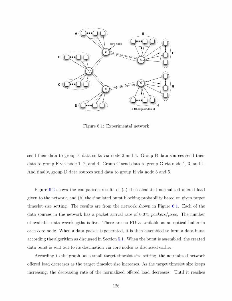
2
1
3
4
5
10 edge nodes
A
B
C
D
E
F
G
H
core node
Figure 6.1: Experimental network
send their data to group E data sinks via node 2 and 4. Group B data sources send their
data to group F via node 1, 2, and 4. Group C send data to group G via node 1, 3, and 4.
And finally, group D data sources send data to group H via node 3 and 5.
Figure 6.2 shows the comparison results of (a) the calculated normalized offered load
given to the network, and (b) the simulated burst blocking probability based on given target
timeslot size setting. The results are from the network shown in Figure 6.1. Each of the
data sources in the network has a packet arrival rate of 0.075 packets/µsec. The number
of available data wavelengths is five. There are no FDLs available as an optical buffer in
each core node. When a data packet is generated, it is then assembled to form a data burst
according the algorithm as discussed in Section 5.1. When the burst is assembled, the created
data burst is sent out to its destination via core nodes as discussed earlier.
According to the graph, at a small target timeslot size setting, the normalized network
offered load decreases as the target timeslot size increases. As the target timeslot size keeps
increasing, the decreasing rate of the normalized offered load decreases. Until it reaches
126
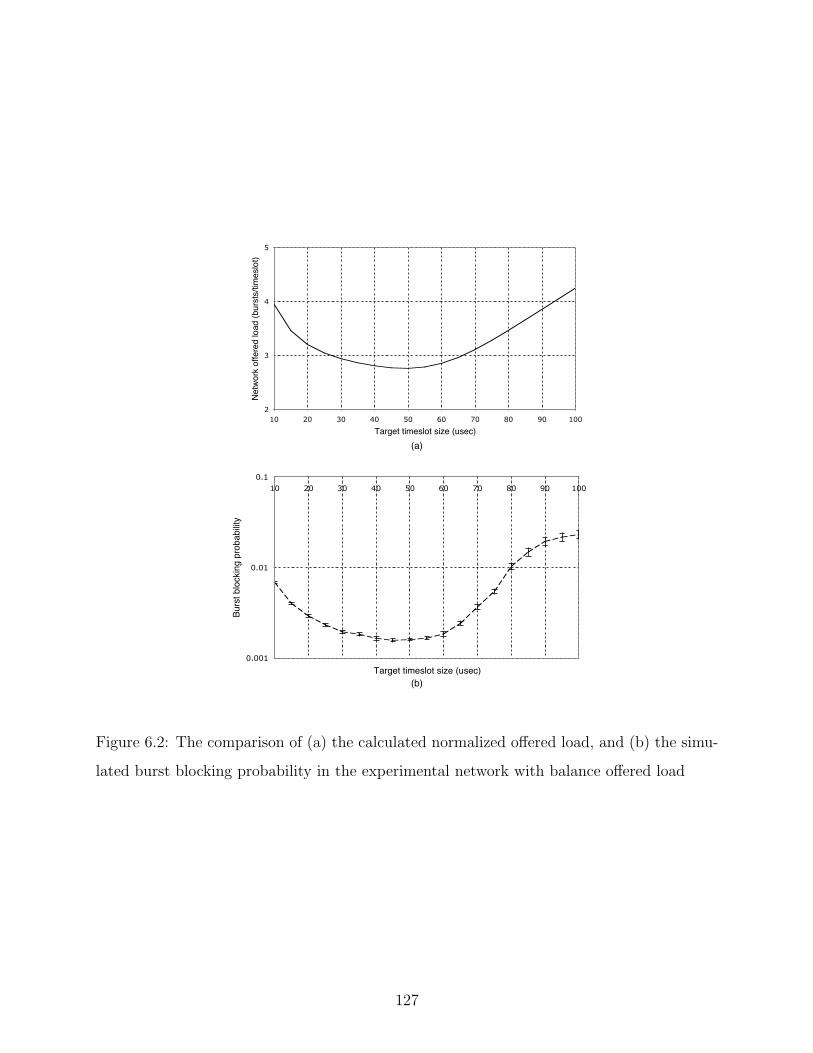
0.001
0.01
0.110 20 30 40 50 60 70 80 90 100
Target timeslot size (usec)
Burs
t blo
ckin
g pr
obab
ility
2
3
4
5
10 20 30 40 50 60 70 80 90 100
Target timeslot size (usec)
Netw
ork
offe
red
load
(bur
sts/
times
lot)
(a)
(b)
Figure 6.2: The comparison of (a) the calculated normalized offered load, and (b) the simu-
lated burst blocking probability in the experimental network with balance offered load
127
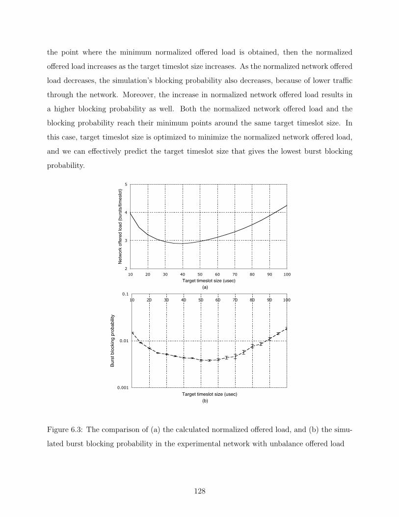
the point where the minimum normalized offered load is obtained, then the normalized
offered load increases as the target timeslot size increases. As the normalized network offered
load decreases, the simulation’s blocking probability also decreases, because of lower traffic
through the network. Moreover, the increase in normalized network offered load results in
a higher blocking probability as well. Both the normalized network offered load and the
blocking probability reach their minimum points around the same target timeslot size. In
this case, target timeslot size is optimized to minimize the normalized network offered load,
and we can effectively predict the target timeslot size that gives the lowest burst blocking
probability.
0.001
0.01
0.110 20 30 40 50 60 70 80 90 100
Target timeslot size (usec)
Burs
t blo
ckin
g pr
obab
ility
2
3
4
5
10 20 30 40 50 60 70 80 90 100
Target timeslot size (usec)
Netw
ork
offe
red
load
(bur
sts/
times
lot)
(a)
(b)
Figure 6.3: The comparison of (a) the calculated normalized offered load, and (b) the simu-
lated burst blocking probability in the experimental network with unbalance offered load
128
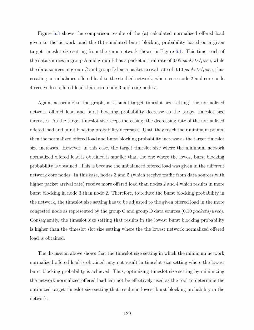
Figure 6.3 shows the comparison results of the (a) calculated normalized offered load
given to the network, and the (b) simulated burst blocking probability based on a given
target timeslot size setting from the same network shown in Figure 6.1. This time, each of
the data sources in group A and group B has a packet arrival rate of 0.05 packets/µsec, while
the data sources in group C and group D has a packet arrival rate of 0.10 packets/µsec, thus
creating an unbalance offered load to the studied network, where core node 2 and core node
4 receive less offered load than core node 3 and core node 5.
Again, according to the graph, at a small target timeslot size setting, the normalized
network offered load and burst blocking probability decrease as the target timeslot size
increases. As the target timeslot size keeps increasing, the decreasing rate of the normalized
offered load and burst blocking probability decreases. Until they reach their minimum points,
then the normalized offered load and burst blocking probability increase as the target timeslot
size increases. However, in this case, the target timeslot size where the minimum network
normalized offered load is obtained is smaller than the one where the lowest burst blocking
probability is obtained. This is because the unbalanced offered load was given in the different
network core nodes. In this case, nodes 3 and 5 (which receive traffic from data sources with
higher packet arrival rate) receive more offered load than nodes 2 and 4 which results in more
burst blocking in node 3 than node 2. Therefore, to reduce the burst blocking probability in
the network, the timeslot size setting has to be adjusted to the given offered load in the more
congested node as represented by the group C and group D data sources (0.10 packets/µsec).
Consequently, the timeslot size setting that results in the lowest burst blocking probability
is higher than the timeslot slot size setting where the the lowest network normalized offered
load is obtained.
The discussion above shows that the timeslot size setting in which the minimum network
normalized offered load is obtained may not result in timeslot size setting where the lowest
burst blocking probability is achieved. Thus, optimizing timeslot size setting by minimizing
the network normalized offered load can not be effectively used as the tool to determine the
optimized target timeslot size setting that results in lowest burst blocking probability in the
network.
129
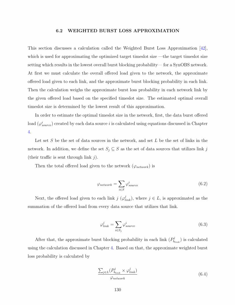
6.2 WEIGHTED BURST LOSS APPROXIMATION
This section discusses a calculation called the Weighted Burst Loss Approximation [42],
which is used for approximating the optimized target timeslot size —the target timeslot size
setting which results in the lowest overall burst blocking probability— for a SynOBS network.
At first we must calculate the overall offered load given to the network, the approximate
offered load given to each link, and the approximate burst blocking probability in each link.
Then the calculation weighs the approximate burst loss probability in each network link by
the given offered load based on the specified timeslot size. The estimated optimal overall
timeslot size is determined by the lowest result of this approximation.
In order to estimate the optimal timeslot size in the network, first, the data burst offered
load (ϕisource) created by each data source i is calculated using equations discussed in Chapter
4.
Let set S be the set of data sources in the network, and set L be the set of links in the
network. In addition, we define the set Sj ⊆ S as the set of data sources that utilizes link j
(their traffic is sent through link j).
Then the total offered load given to the network (ϕnetwork) is
ϕnetwork =∑i∈S
ϕisource (6.2)
Next, the offered load given to each link j (ϕjlink), where j ∈ L, is approximated as the
summation of the offered load from every data source that utilizes that link.
ϕjlink =∑i∈Sj
ϕisource (6.3)
After that, the approximate burst blocking probability in each link (P jblink
) is calculated
using the calculation discussed in Chapter 4. Based on that, the approximate weighted burst
loss probability is calculated by
∑j∈L(P j
blink× ϕjlink)
ϕnetwork(6.4)
130
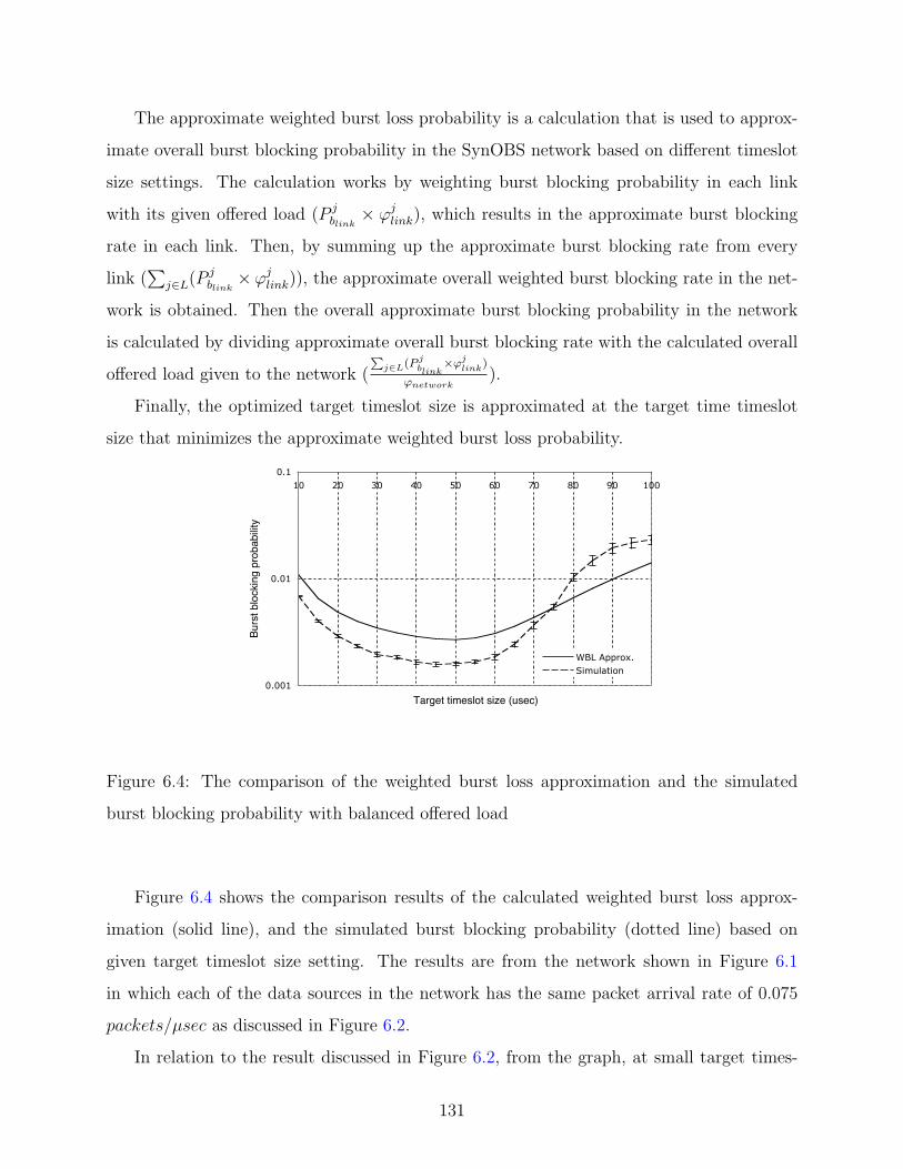
The approximate weighted burst loss probability is a calculation that is used to approx-
imate overall burst blocking probability in the SynOBS network based on different timeslot
size settings. The calculation works by weighting burst blocking probability in each link
with its given offered load (P jblink× ϕjlink), which results in the approximate burst blocking
rate in each link. Then, by summing up the approximate burst blocking rate from every
link (∑
j∈L(P jblink× ϕjlink)), the approximate overall weighted burst blocking rate in the net-
work is obtained. Then the overall approximate burst blocking probability in the network
is calculated by dividing approximate overall burst blocking rate with the calculated overall
offered load given to the network (Pj∈L(P jblink
×ϕjlink)ϕnetwork
).
Finally, the optimized target timeslot size is approximated at the target time timeslot
size that minimizes the approximate weighted burst loss probability.
0.001
0.01
0.110 20 30 40 50 60 70 80 90 100
Target timeslot size (usec)
Burs
t blo
ckin
g pr
obab
ility
WBL Approx.Simulation
Figure 6.4: The comparison of the weighted burst loss approximation and the simulated
burst blocking probability with balanced offered load
Figure 6.4 shows the comparison results of the calculated weighted burst loss approx-
imation (solid line), and the simulated burst blocking probability (dotted line) based on
given target timeslot size setting. The results are from the network shown in Figure 6.1
in which each of the data sources in the network has the same packet arrival rate of 0.075
packets/µsec as discussed in Figure 6.2.
In relation to the result discussed in Figure 6.2, from the graph, at small target times-
131
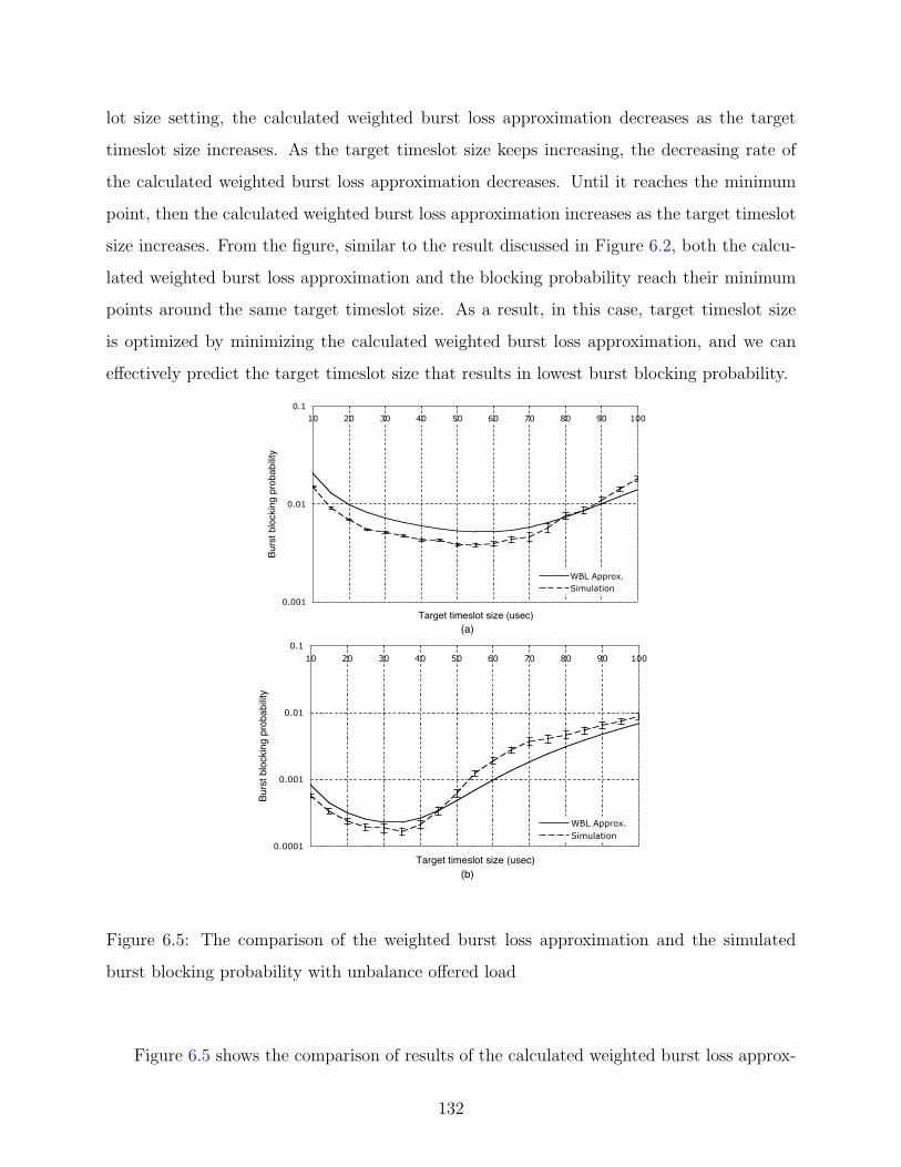
lot size setting, the calculated weighted burst loss approximation decreases as the target
timeslot size increases. As the target timeslot size keeps increasing, the decreasing rate of
the calculated weighted burst loss approximation decreases. Until it reaches the minimum
point, then the calculated weighted burst loss approximation increases as the target timeslot
size increases. From the figure, similar to the result discussed in Figure 6.2, both the calcu-
lated weighted burst loss approximation and the blocking probability reach their minimum
points around the same target timeslot size. As a result, in this case, target timeslot size
is optimized by minimizing the calculated weighted burst loss approximation, and we can
effectively predict the target timeslot size that results in lowest burst blocking probability.
0.0001
0.001
0.01
0.110 20 30 40 50 60 70 80 90 100
Target timeslot size (usec)
Burs
t blo
ckin
g pr
obab
ility
WBL Approx.Simulation
0.001
0.01
0.110 20 30 40 50 60 70 80 90 100
Target timeslot size (usec)
Burs
t blo
ckin
g pr
obab
ility
WBL Approx.Simulation
(a)
(b)
Figure 6.5: The comparison of the weighted burst loss approximation and the simulated
burst blocking probability with unbalance offered load
Figure 6.5 shows the comparison of results of the calculated weighted burst loss approx-
132
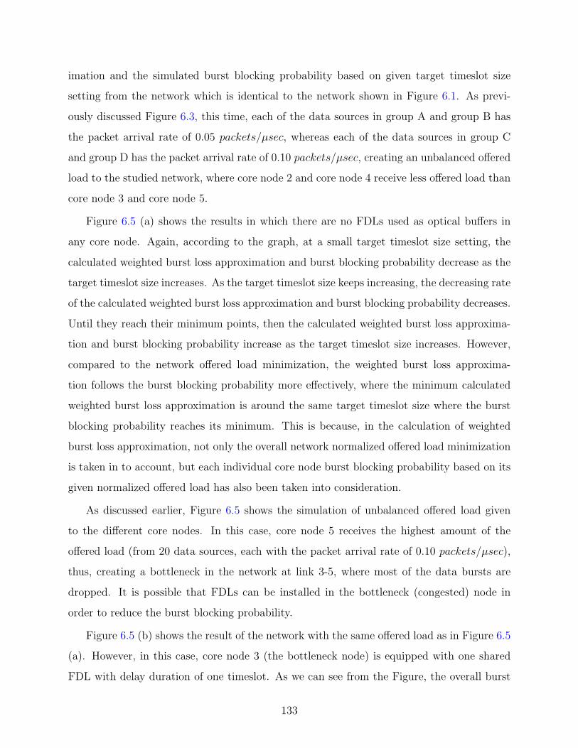
imation and the simulated burst blocking probability based on given target timeslot size
setting from the network which is identical to the network shown in Figure 6.1. As previ-
ously discussed Figure 6.3, this time, each of the data sources in group A and group B has
the packet arrival rate of 0.05 packets/µsec, whereas each of the data sources in group C
and group D has the packet arrival rate of 0.10 packets/µsec, creating an unbalanced offered
load to the studied network, where core node 2 and core node 4 receive less offered load than
core node 3 and core node 5.
Figure 6.5 (a) shows the results in which there are no FDLs used as optical buffers in
any core node. Again, according to the graph, at a small target timeslot size setting, the
calculated weighted burst loss approximation and burst blocking probability decrease as the
target timeslot size increases. As the target timeslot size keeps increasing, the decreasing rate
of the calculated weighted burst loss approximation and burst blocking probability decreases.
Until they reach their minimum points, then the calculated weighted burst loss approxima-
tion and burst blocking probability increase as the target timeslot size increases. However,
compared to the network offered load minimization, the weighted burst loss approxima-
tion follows the burst blocking probability more effectively, where the minimum calculated
weighted burst loss approximation is around the same target timeslot size where the burst
blocking probability reaches its minimum. This is because, in the calculation of weighted
burst loss approximation, not only the overall network normalized offered load minimization
is taken in to account, but each individual core node burst blocking probability based on its
given normalized offered load has also been taken into consideration.
As discussed earlier, Figure 6.5 shows the simulation of unbalanced offered load given
to the different core nodes. In this case, core node 5 receives the highest amount of the
offered load (from 20 data sources, each with the packet arrival rate of 0.10 packets/µsec),
thus, creating a bottleneck in the network at link 3-5, where most of the data bursts are
dropped. It is possible that FDLs can be installed in the bottleneck (congested) node in
order to reduce the burst blocking probability.
Figure 6.5 (b) shows the result of the network with the same offered load as in Figure 6.5
(a). However, in this case, core node 3 (the bottleneck node) is equipped with one shared
FDL with delay duration of one timeslot. As we can see from the Figure, the overall burst
133
blocking probability is reduced compared to the result when node 3 has no FDLs installed. In
addition, the timeslot size setting in which the lowest burst blocking probability is obtained
becomes smaller than when there are no FDLs available in the node. This is because, when
there is an FDL available for buffering data bursts in the bottleneck node (node 3), the
burst blocking in the bottleneck node is greatly reduced. Since the ratio of blocked data
bursts in the bottleneck node to overall network blocked data bursts is greatly reduced, the
ratio of blocked data bursts in node 2 to overall blocked data bursts in the network becomes
more significant. Because node 2 receives the traffic from 20 data sources, each with the
packet arrival rate of 0.05 packets/µsec, as opposed to the 0.10 packets/µsec given to node
3, the timeslot size setting, in which the lowest burst blocking probability is obtained, is
moved toward the optimizing point of the packet arrival rate of node 2 data sources (0.05
packets/µsec).
As we can see from the Figure, as the node configurations in the network have been
changed, the result from the calculated weighted burst loss approximation closely follows
the change of the simulated burst blocking probability in the network. This is because
each of the individual network node configurations has also been considered in the weight
burst loss approximation calculation, where, with the same offered load, the different node
configurations result in the different burst blocking probability in the node. Therefore,
this shows that, in addition to the ability to adapt to the unbalance offered load given to
different nodes in the network, the weighted burst loss approximation is also able to adapt
to the different individual node configurations in the network.
6.2.1 Weight Burst Loss Approximation in Large Network
In this study, the vBNS network topology [43] (shown in Figure 6.6) has been used as the
studied network. The vBNS network topology has twelve core nodes, geographically located
in different cities across the United States. If the network used SynOBS, then, with each of
the core nodes, there would be one edge node, which is co-located and directly connected to
it. These edge nodes act as a traffic sources and traffic sinks to/from the SynOBS network.
Let’s provide full connectivity, with two classes of traffic between every pair of edge nodes.
134
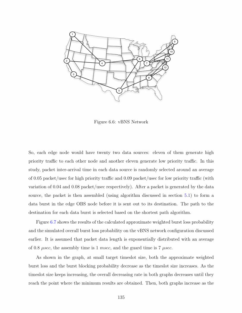
74
9
10
116
12
1
2
3
5
8
Figure 6.6: vBNS Network
So, each edge node would have twenty two data sources: eleven of them generate high
priority traffic to each other node and another eleven generate low priority traffic. In this
study, packet inter-arrival time in each data source is randomly selected around an average
of 0.05 packet/usec for high priority traffic and 0.09 packet/usec for low priority traffic (with
variation of 0.04 and 0.08 packet/usec respectively). After a packet is generated by the data
source, the packet is then assembled (using algorithm discussed in section 5.1) to form a
data burst in the edge OBS node before it is sent out to its destination. The path to the
destination for each data burst is selected based on the shortest path algorithm.
Figure 6.7 shows the results of the calculated approximate weighted burst loss probability
and the simulated overall burst loss probability on the vBNS network configuration discussed
earlier. It is assumed that packet data length is exponentially distributed with an average
of 0.8 µsec, the assembly time is 1 msec, and the guard time is 7 µsec.
As shown in the graph, at small target timeslot size, both the approximate weighted
burst loss and the burst blocking probability decrease as the timeslot size increases. As the
timeslot size keeps increasing, the overall decreasing rate in both graphs decreases until they
reach the point where the minimum results are obtained. Then, both graphs increase as the
135
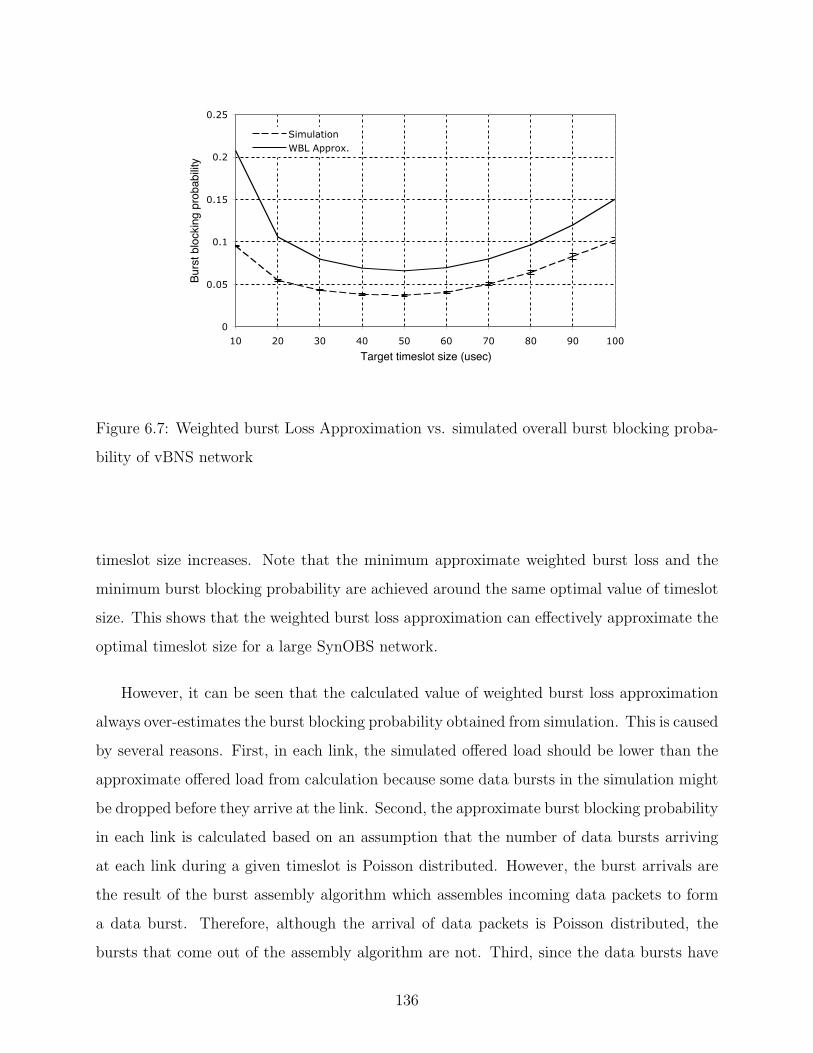
0
0.05
0.1
0.15
0.2
0.25
10 20 30 40 50 60 70 80 90 100
Target timeslot size (usec)
Burs
t blo
ckin
g pr
obab
ility
SimulationWBL Approx.
Figure 6.7: Weighted burst Loss Approximation vs. simulated overall burst blocking proba-
bility of vBNS network
timeslot size increases. Note that the minimum approximate weighted burst loss and the
minimum burst blocking probability are achieved around the same optimal value of timeslot
size. This shows that the weighted burst loss approximation can effectively approximate the
optimal timeslot size for a large SynOBS network.
However, it can be seen that the calculated value of weighted burst loss approximation
always over-estimates the burst blocking probability obtained from simulation. This is caused
by several reasons. First, in each link, the simulated offered load should be lower than the
approximate offered load from calculation because some data bursts in the simulation might
be dropped before they arrive at the link. Second, the approximate burst blocking probability
in each link is calculated based on an assumption that the number of data bursts arriving
at each link during a given timeslot is Poisson distributed. However, the burst arrivals are
the result of the burst assembly algorithm which assembles incoming data packets to form
a data burst. Therefore, although the arrival of data packets is Poisson distributed, the
bursts that come out of the assembly algorithm are not. Third, since the data bursts have
136
to traverse through multiple hops in the network, the burst blocking in previous links might
have the effect of smoothing out the burst arrivals in later links. While the Weighted Burst
Loss Approximation is not suitable for predicting the actual burst blocking probability in
SynOBS network, it can effectively predict the optimized target timeslot size where the
minimum burst blocking probability is achieved.
In this dissertation, in addition to the network configuration discussed above, several
network configurations, along with different given network offered load patterns have been
tested to confirm the effectiveness of Weighted Burst Loss Approximation for approximating
the optimal timeslot size setting in SynOBS network.
6.2.2 Simulated Weight Burst Loss Approximation
In the SynOBS network with adaptive timeslot size implemented (the timeslot size set-
ting can be dynamically changed according to current network condition), the real-time
approximation of the optimized timeslot size is neccesary. Since there are different FDL
configurations in a core node, some of the FDL configurations might not be suitable for the
real-time calculation of the node’s burst blocking probability used in the weighted burst loss
approximation. For example, some of these FDL configurations might include the SynOBS
core node with shared FDLs that have large number of ports and FDLs. This results in large
number (hundreds) of states in the discrete-time Markov model (discussed in Chapter 4), in
which lots of computational power and computational time are required. Another example
is a SynOBS core node equipped with different multiple-length FDLs (discussed in section
4.6), which in this case, the mathematical formulation of the burst blocking probability in
the core node might be too complicated to analyze.
To overcome the difficulty discussed above, each individual node burst blocking proba-
bility used by the weighted burst loss approximation can be pre-calculated or pre-simulated
based on various offered loads given to the node. Then these predetermined individual node
blocking probabilities are stored in a central database. During the realtime network oper-
ation, based on each of the node configurations in the network and the calculated offered
load, their pre-calculated/simulated burst blocking probability can be retrieved from the
137
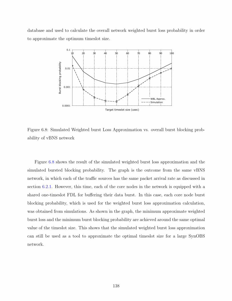
database and used to calculate the overall network weighted burst loss probability in order
to approximate the optimum timeslot size.
0.0001
0.001
0.01
0.110 20 30 40 50 60 70 80 90 100
Target timeslot size (usec)
Burs
t blo
ckin
g p
robab
ility
WBL Approx.Simulation
Figure 6.8: Simulated Weighted burst Loss Approximation vs. overall burst blocking prob-
ability of vBNS network
Figure 6.8 shows the result of the simulated weighted burst loss approximation and the
simulated bursted blocking probability. The graph is the outcome from the same vBNS
network, in which each of the traffic sources has the same packet arrival rate as discussed in
section 6.2.1. However, this time, each of the core nodes in the network is equipped with a
shared one-timeslot FDL for buffering their data burst. In this case, each core node burst
blocking probability, which is used for the weighted burst loss approximation calculation,
was obtained from simulations. As shown in the graph, the minimum approximate weighted
burst loss and the minimum burst blocking probability are achieved around the same optimal
value of the timeslot size. This shows that the simulated weighted burst loss approximation
can still be used as a tool to approximate the optimal timeslot size for a large SynOBS
network.
138
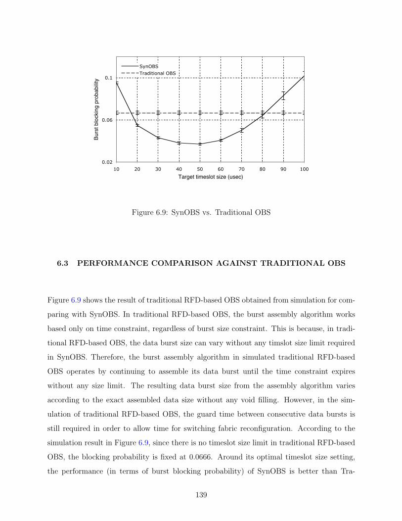
0.02
0.06
0.1
10 20 30 40 50 60 70 80 90 100
Target timeslot size (usec)
Burs
t blo
ckin
g pr
obab
ility
SynOBSTraditional OBS
Figure 6.9: SynOBS vs. Traditional OBS
6.3 PERFORMANCE COMPARISON AGAINST TRADITIONAL OBS
Figure 6.9 shows the result of traditional RFD-based OBS obtained from simulation for com-
paring with SynOBS. In traditional RFD-based OBS, the burst assembly algorithm works
based only on time constraint, regardless of burst size constraint. This is because, in tradi-
tional RFD-based OBS, the data burst size can vary without any timslot size limit required
in SynOBS. Therefore, the burst assembly algorithm in simulated traditional RFD-based
OBS operates by continuing to assemble its data burst until the time constraint expires
without any size limit. The resulting data burst size from the assembly algorithm varies
according to the exact assembled data size without any void filling. However, in the sim-
ulation of traditional RFD-based OBS, the guard time between consecutive data bursts is
still required in order to allow time for switching fabric reconfiguration. According to the
simulation result in Figure 6.9, since there is no timeslot size limit in traditional RFD-based
OBS, the blocking probability is fixed at 0.0666. Around its optimal timeslot size setting,
the performance (in terms of burst blocking probability) of SynOBS is better than Tra-
139
ditional RFD-based OBS. However, with poor timeslot size setting, where it is set to be
either too large or too small, the performace of SynOBS can degrade until its performance
becomes worsen than traditional RFD-based OBS because this poor timeslot size setting
results in poor resource utilization in SynOBS. As a result, this analysis shows that timeslot
size setting in SynOBS networks must be carefully designed in order to gain the advantage of
the synchronized timeslot-based approach and obtain better performance in terms of burst
blocking probability over the traditional asynchronous RFD-based OBS.
140
7.0 CONCLUSIONS AND FUTURE WORK
This dissertation provides comprehensive studies of a synchronized timeslot-based OBS,
which is referred to as Time-Synchronized Optical Burst Switching (SynOBS). The SynOBS
protocol is proposed with two main considerations in mind. First, it allows a less complex
optical switching fabric to be employed in the core OBS nodes rather than the more com-
plex switching fabric required in traditional OBSs. Second, it utilizes the timeslot-based
mechanism in order to achieve better performance than that of traditional OBSs.
Although they are not the main focus of this dissertation, some of the basic physical
implementation ideas of a SynOBS node have been briefly studied and discussed. One of
the important aspects of SynOBS that is different from the traditional OBS is synchro-
nization, where the mechanism of realigning and synchronizing incoming data streams from
different incoming ports and wavelengths is mandatory. For SynOBS, timeslot synchroniz-
ers and wavelength delay variation compensators are used to synchronize these incoming
data streams. The timeslot synchronizers are responsible for realigning the different incom-
ing data streams from different incoming ports that arrive out of phase compared to each
other. In addition, due to the variation of the wave’s speed among different wavelengths, the
wavelength delay variation compensators are used to realign these out-of-phase data streams
among different data wavelengths within the same incoming port.
In this dissertation, the performance analysis of a SynOBS core node with several FDL
reservation mechanisms is discussed, including the performance analysis of a SynOBS core
node without FDLs, a SynOBS core node with separated FDLs, SynOBS core node with
Shared FDLs, and later, a SynOBS core node with multiple-length FDLs. Regarding the
results from our study, while simulations comparing SynOBS and traditional OBS shows
promising results for SynOBS over traditional OBS in every reservation algorithm, SynOBS
141
with shared FDLs promises better performance for overall burst-drop probability, as com-
pared to SynOBS with separated FDLs. Furthermore, because the multiple-length FDL
configuration provides a greater variety of possible delay durations and allows more data
bursts to be delayed in the core node, the blocking performance of multiple-length FDL
configurations are better than that of the fixed length one timeslot configurations.
While employing a synchronized timeslot based mechanism in SynOBS provides an op-
portunity to achieve better resource utilization than traditional OBS, such a system has
to be carefully designed in order to achieve the best performance possible. The effect of
timeslot size setting causes a trade-off between the burst assembly time constraint and the
duration of guard time between each consecutive timeslot, basically because the SynOBS is
based on fixed size timeslot mechanism. This study shows that the timeslot size setting in
SynOBS networks must be carefully chosen in order to achieve the best timeslot utilization
as possible, which subsequently results in a better burst blocking probability in the network.
In order to optimize the timeslot size setting in a SynOBS network, first the minimized
normalized offered load (bursts/timeslot) given to the entire network (the timeslot size setting
in which results in the minimum nomalized offered load) is considered. Due to the unbalanced
offered load given to the different network core nodes, the timeslot size setting in which the
minimum network normalized offered load is obtained may not result in timeslot size setting
where the lowest burst blocking probability is achieved. Thus, optimizing timeslot size
setting by minimizing the network normalized offered load can not be effectively used as the
tool to determine the optimized target timeslot size setting that results in the lowest burst
blocking probability in the network.
Then, an analytical framework called the Weighted Burst Loss Approximation which
can effectively approximate the optimal timeslot size —the target timeslot size setting in
which results in the lowest overall burst blocking probability— for a SynOBS network has
been discussed. In the Weighted Burst Loss Approximation, initially, the overall offered load
given to the network, the approximate offered load given to each link, and the approximate
burst blocking probability in each link are obtained (either by calculation or simulation).
Subsequently, the analysis weighs the approximate burst loss probability in each network
link by the given offered load based on the given timeslot size. The approximate optimized
142
overall timeslot size is determined by the lowest result of this approximation. Although the
Weighted Burst Loss Approximation is not suitable for predicting the actual burst blocking
probability in a SynOBS network, it can effectively estimate the optimal timeslot size where
the minimum burst blocking probability can be achieved.
Finally, the performance comparison (in terms of burst blocking probability) between
SynOBS and traditional RFD-based OBS in a large network has been provided in this
dissertation. According to the result, the performance of SynOBS with the near-optimal
timeslot size setting is better than the Traditional RFD-based OBS. However, with poor
timeslot size setting (too large or too small size setting), the performace of SynOBS can
become worse than the traditional OBS because this inappropriate timeslot size setting
results in poor resource utilization in SynOBS. In conclusion, the timeslot size in the SynOBS
network has to be chosen in order to gain the advantage of the synchronized timeslot-based
approach and obtain better performance in terms of burst blocking probability over the
traditional asynchronous RFD-based OBS.
While many aspects of the SynOBS have been discussed and studied thoroughly in
this dissertation, in order to gain better understanding and achieve better performance in
SynOBS networks, several issues remain to be studied. This further research includes:
• The fairness issue in SynOBS core node with shared FDLs:
As discussed earlier in this dissertation, while a SynOBS core node with shared FDLs can
effectively utilize the available FDLs in a core node, unbalanced offered loads may result
in an unfair FDL utilization among the output ports, where the traffic from the output
port with higher given offered load tends to over utilize the shared FDLs, compared
with the traffic from the output port with lower given offered load. Therefore, the FDL
reservation algorithm for SynOBS with shared FDLs has to be carefully redesigned in
order to avoid such a problem.
• The detailed analysis of SynOBS core node with multiple length FDLs:
This dissertation has discussed the possible advantages of employing multiple length
FDLs over fixed length one timeslot FDLs in the core node. Some of its aspects have
been discussed, including cost analysis and FDL reservation algorithm, as well as several
FDL configurations (using simulation). However, in order to gain better understanding
143
about the effect of different FDL configurations to their blocking performances, detailed
analysis of SynOBS core nodes with multiple length FDLs should be studied in further
research.
• The improvement of the weighted burst loss approximation:
Although, currently, the weighted burst loss approximation algorithm can effectively
approximate the optimal timeslot size setting in the SynOBS network, as discuss earlier,
the weight burst loss approximation can not be effectively used for predicting the actual
burst blocking probability in SynOBS network. In order to predict more accurate burst
blocking probability (which in turn, provides an even more accurate optimal timeslot size
approximation), several aspects have to be taken into the calculation. These include, but
not limited to, a more accurate approximate link offered load, considering burst loss in the
intermediate node, using the more appropriate burst arrival process (Poisson is currently
assumed), and analyzing the burst smoothing effect of burst arrivals after traversing
through multiple hops in the network.
• The weighted packet loss approximation:
In this dissertation, the optimal timeslot size is assumed as the timeslot size at which
the lowest burst blocking probability in the SynOBS network is obtained (the weighted
burst loss approximation). However, since a data burst is a result of the assembled
data packets that have the same destination and priority, and since the number of data
packets in each of the data burst can be varied, the timeslot size that results in the
lowest burst blocking probability may not cause the lowest packet loss in the network.
In further research, the extension of the weighted burst loss approximation should also
be considered and studied. Despite assuming that the lowest burst blocking probability
is the optimal timeslot size, further analysis should be extended by assuming that the
timeslot size in which the lowest end to end packet loss probability is obtained as the
optimal timeslot size.
• The detailed study of possible physical implementation of SynOBS system:
Although some discussion of the possible physical implementation of the SynOBS sys-
tem has been provided in this dissertation, the detailed characteristics of every physical
element still have to be taken into consideration for the detailed system design. For
144
example, some of the physical elements (e.g. Erbium-Doped Fiber Amplifiers) require
constant presence of signal for them to operate normally and the presence of guard-time
and void filling might cause some of these physical elements to not work properly. This
problem (as well as other possible physical limitations) has to be considered in further
research.
145
BIBLIOGRAPHY
[1] J. Ramamirtham and J. Turner. Time sliced optical burst switching. In Proceedings ofINFOCOMM, 3:2030–2038, 2003.
[2] X. Yu, Y. Chen, and C. Qiao. A study of traffic statistic of assembled burst traf-fic in optical burst switched networks. SPIE Optical Networking and CommunicationConference (OptiComm) 2002, 2002.
[3] A. Banerjee, J. Drake, J. P. Lang, and B. Turner. Optical packet switching in corenetworks: Between vision and reality. IEEE Communications Magazine, pages 60–65,September 2002.
[4] C. Qiao. Labeled optical burst switching for ip-over-wdm integration. IEEE Commu-nications Magazine, pages 104–114, September 2000.
[5] J. S. Turner. Terabit burst switching. Tech, Rep. WUCS-97-49, December 1997.
[6] D. K. Hunter and I. Andonovic. Approaches to optical internet packet switching. IEEECommunications Magazine, pages 116–122, September 2000.
[7] T. S. El-Baweb and J. Shin. Optical packet switching in core networks: Between visionand reality. IEEE Communications Magazine, pages 60–65, September 2002.
[8] C. Qiao and M. Yoo. Choices, feature and issue in optical burst switching. OpticalNetwork Magazine 1, pages 36–44, April 2000.
[9] L. Xu, H. G. Perros, and G. Rouskas. Techniques for optical packet switching and opticalburst switching. IEEE Communications Magazine, pages 136–142, January 2001.
[10] R. Ramaswani and K. N. Sivarajan. Optical Networks: A Practical Perspective. MorganKaufman Publishers Inc., 1998.
[11] I. Kaminow and T. Li. Optical fiber Telecommunications IVA, Components. AcademicPress.
[12] D. Hunter, D.Cornwell, T. H. Gilfedder, A. Franzen, and I. Andonovic. Slob: A switchwith large optical buffers for packet switching. Journal of Lightwave Technology, 16(10),October 1998.
146
[13] R. A. Thompson and D. K. Hunter. Elementary photonic switching modules in threedevisions. IEEE Journal on Selected Areas in Communications, 14(2), February 1996.
[14] A. Pattavina. Architectures and performance of optical packet switching nodes for ipnetworks. Journal of Lightwave Technology, 23(3), 2005.
[15] S. Bjornstad, M. Nord, and C. M. Gauger. Optical burst and packet switching: Nodeand network design, contention resolution and quality of service. Telecommunications,2003. ConTEL 2003. Proceedings of the 7th International Conference, 2:775– 782, June2003.
[16] G. I. Papadimitriou, C. Papazoglou, and A. S. Promportsis. Optical switching: Switchfabrics, techniques, and architectures. Journal of Lightwave Technology, 21(2), Febuary2003.
[17] J.Y. Wei and R.I. McFarland. Just-in-time signaling for wdm optical burst switchingnetworks. Journal of Lightwave Technology, December 2000.
[18] M. Yoo and C. Qiao. Just-enough-time (jet): A high speed protocol for bursty trafficin optical networks. In proceeding of IEEE/LEOS Conf. on Technologies For a GlobalInformation Infrastructure, August 1997.
[19] K. Dolzer, C. Gauger, J. Spath, and S. Bodamer. Evaluation of reservation mechanismsfor optical burst switching. AEU Int. J. Electron. Commun., 55(1), 2001.
[20] H. L. Vu and M Zukerman. Blocking probability for priority classes in optical burstswitching networks. IEEE Communications Letters, 6(5):214–216, May 2002.
[21] F. Farahmand, V. M. Vokkarane, and J. P. Jue. Practical priority contention resolutionfor slotted optical burst switching networks. at the first WOBS.
[22] M. Yoo, C. Qiao, and S. Dixit. Qos performance of optical burst switching in ip-over-wdm networks. IEEE Journal on Selected Areas in Communications, October 2000.
[23] R. A. Thompson. Telephone Switching Systems. Artech House Inc.
[24] C. M. Gauger. Dimensioning of fdl buffers for optical burst switching nodes. Proceedingsof the 6th IFIP Working Conference on Optical Network Design and Modeling (ONDM2002), February 2002.
[25] V. M. Vokkarane, J. P. Jue, and S. Sitaraman. Burst segmentation: An approch forreducing paket loss in optical burst switched networks. UTD Technical Report UTDCS-20-01, September 2001.
[26] N. Abramson. The aloha system — another alternative for computer communications.AFIPS Conference Proceedings, 36, 295–298 1970.
147
[27] L. Roberts. Aloha packet system with and without slots and capture. Stanford ResearchInstitute, Advanced Research Projects work Information Center, 1972.
[28] M. R. Vastag. Answers to your question, corning incorporated,http://www.corning.com/opticalfiber/guidelines magazine/archived issues/winter 2001/r3521.pdf.
[29] S. Shaari and K. Kandiah. Beam propagation method study of wavelength dependent in-directional coupler switch. Semiconductor Electronics, 1998. Proceedings. ICSE apos;98.1998 IEEE International Conference, pages 223–228, 1998.
[30] A. Pattavina, M. Rebughini, and A. Sipone. Performance of awg-based optical nodeswith shared tunable wavelength converters. In Proceedings of Global TelecommunicationsConference, 2005. GLOBECOM ’05. IEEE, December 2005.
[31] V. Eramo and M. Listanti. Packet loss in a bufferless optical wdm switch employingshared tuneable wavelength converters. J. Lightwave Technol., 18:1818–1833, December2000.
[32] G. Keiser. Optical Communications Essentials. McGraw-Hill.
[33] A. Rugsachart and R. A. Thompson. An analysis of time-synchronized optical burstswitching. 2006 Workshop on High Performance Switching and Routing, June 2006.
[34] Hou T.-C. and Wong A.K. Queueing analysis for atm switching of mixed continuous-bit-rate and bursty traffic. INFOCOM ’90 Proceedings, IEEE, June 1990.
[35] Ng C.H., Zhang L., Cheng T.H., and Tan C.H. Cell loss probability of a finite atmbuffer queue. Communications, IEE Proceedings, Febuary 1999.
[36] J. Kim and C. Jun. An exact performance analysis of an atm multiplexer loaded withheterogeneous on-off sources. ATM (ICATM 2001) and High Speed Intelligent InternetSymposium, 2001. Joint 4th IEEE International Conference, April 2001.
[37] D. Gross and C. M. Harris. Fundamentals of Queueing Theory -3rd edition. Probabilityand Statistics. Wiley.
[38] N. Endo, T. Ohuchi, T. Kozaki, H. Kuwahara, and M. Mori. Traffic characteristicsevaluation of a shared buffer atm switch. Global Telecommunications Conference, 1990,and Exhibition. ’Communications: Connecting the Future’, GLOBECOM ’90., IEEE,3:1913–1918, Dec 1990.
[39] F. Kamoun and L. Kleinrock. Analysis of shared finite storage in a computer networknode environment under general traffic conditions. IEEE Transactions on Communica-tions, 28(7), July 1980.
148
[40] A.E. Eckberg and T.-C. Hou. Effects of output buffer sharing on buffer requirementsin an atdmpacket switching. INFOCOM ’88. Networks: Evolution or Revolution? Pro-ceedings. Seventh Annual Joint Conference of the IEEE Computer and CommuncationsSocieties., IEEE, (459-466), March 1988.
[41] Y. Xiong, M. Vandenhoute, and H. C. Cankaya. Control archtecutre in optical burstswtiched wdm networks. IEEE JSAC, 18(10):1838–1851, October 2000.
[42] A. Rugsachart and R. A. Thompson. Optimal timeslot size for synchronous opticalburst switching. In International Workshop on Optical Burst/Packet Switching, FourthInternational Conference on Broadband Communications, Networks, and System (IEEEBROADNETS 2007), September 2007.
[43] http://www.it.northwestern.edu/metrochicago/intro.htm. June 2007.
149