Time Synchronization in Wireless Sensor Networksethesis.nitrkl.ac.in/5791/1/E-7.pdf · ·...
43
Time Synchronization in Wireless Sensor Networks Sikandar Kumar Department of Computer Science and Engineering National Institute of Technology Rourkela Rourkela-769 008, Odisha, India June 2014
-
Upload
trankhuong -
Category
Documents
-
view
241 -
download
3
Transcript of Time Synchronization in Wireless Sensor Networksethesis.nitrkl.ac.in/5791/1/E-7.pdf · ·...

Time Synchronization
in
Wireless Sensor Networks
Sikandar Kumar
Department of Computer Science and Engineering
National Institute of Technology Rourkela
Rourkela-769 008, Odisha, India
June 2014

Time Synchronization
in
Wireless Sensor Networks
Thesis submitted in partial fulfillment of the requirements for the degree of
Master of Technology
in
Computer Science and Engineering(Specialization: Information Security)
by
Sikandar Kumar(Roll No.- 212cs2108)
under the supervision of
Prof. Manmath Narayan Sahoo
Department of Computer Science and Engineering
National Institute of Technology Rourkela
Rourkela, Odisha, 769 008, India
June 2014

Department of Computer Science and EngineeringNational Institute of Technology RourkelaRourkela-769 008, Odisha, India.
Certificate
This is to certify that the work in the thesis entitled Time Synchronization in
Wireless Sensor Networks by Sikandar Kumar is a record of an original
research work carried out by him under my supervision and guidance in partial
fulfillment of the requirements for the award of the degree of Master of Technology
with the specialization of Information Security in the department of Computer
Science and Engineering, National Institute of Technology Rourkela. Neither this
thesis nor any part of it has been submitted for any degree or academic award
elsewhere.
Place: NIT Rourkela (Prof. Manmath Narayan Sahoo)Date: June 2, 2014 CSE Department
NIT Rourkela, Odisha

Acknowledgment
I am grateful to numerous local and global peers who have contributed towards
shaping this thesis. At the outset, I would like to express my sincere thanks to
Prof. Manmath Narayan Sahoo for his advice during my thesis work. As my
supervisor, he has constantly encouraged me to remain focused on achieving my
goal. His observations and comments helped me to establish the overall direction
to the research and to move forward with investigation in depth. He has helped
me greatly and been a source of knowledge.
I am very much indebted to Prof. Manmath Narayan Sahoo for his continuous
encouragement and support. He is always ready to help with a smile. I am also
thankful to all the professors at the department for their support.
I would like to thank all my friends and lab-mates for their encouragement and
understanding. Their help can never be penned with words.
I must acknowledge the academic resources that I have got from NIT Rourkela.
I would like to thank administrative and technical staff members of the Department
who have been kind enough to advise and help in their respective roles.
Last, but not the least, I would like to dedicate this thesis to my family, for
their love, patience, and understanding.
Sikandar kumar
Roll-212cs2108

Author’s Declaration
I hereby declare that all work contained in this report is my own work unless
otherwise acknowledged. Also, all of my work has not been submitted for any
academic degree. All sources of quoted information has been acknowledged by
means of appropriate reference. If any means of plagiarism is found in future, I
shall be held responsible.
Sikandar Kumar
Roll: 212CS2108
Department of Computer Science

Abstract
Time synchronization is a basic requirement for various applications in wireless
sensor network, e.g., event detection, speed estimating, environment monitoring,
data aggregation, target tracking, scheduling and sensor nodes cooperation. Time
synchronization is also helpful to save energy in WSN because it provides the
possibility to set nodes into the sleeping mode. In wireless sensor networks all
of above applications need that all sensor nodes have a common time reference.
However, most existing time synchronization protocols are likely to deteriorate or
even be destroyed when the WSNs attack by malicious intruders. The recently
developed maximum and minimum consensus based time synchronization protocol
(MMTS) is a promising alternative as it does not depend on any reference node
or network topology. But MMTS is vulnerable to message manipulation attacks.
In this thesis, we focus on how to defend the MMTS protocol in wireless sen-
sor networks under message manipulation attacks. We investigate the impact of
message manipulation attacks over MMTS. Then, a novel Secured Maximum and
Minimum Consensus based Time Synchronization (SMMTS) protocol is proposed
to detect and invalidate message manipulation attacks.
Keywords: wireless sensor network, time synchronization, maximum consensus,
minimum consensus, message manipulation attack.

Contents
Certificate ii
Acknowledgement iii
Declaration iv
Abstract v
Abbreviations viii
List of Figures i
1 Introduction 1
1.1 Wireless Sensor Network . . . . . . . . . . . . . . . . . . . . . . . . 1
1.1.1 Applications of sensor networks . . . . . . . . . . . . . . . . 1
1.2 Overview of Time Synchronization in WSN . . . . . . . . . . . . . . 3
1.2.1 Reasons for time synchronization . . . . . . . . . . . . . . . 3
1.2.2 Common Challenges for Synchronization Methods . . . . . . 5
1.2.3 Metrics for Evaluating Time Synchronization Schemes . . . . 6
1.2.4 Clocks in Computer . . . . . . . . . . . . . . . . . . . . . . . 6
1.2.5 Clock Model . . . . . . . . . . . . . . . . . . . . . . . . . . . 8
1.2.6 Attack Model . . . . . . . . . . . . . . . . . . . . . . . . . . 9
2 Literature review 10
3 Maximum and Minimum Consensus based Time Synchronization 16
3.1 MMTS under attack . . . . . . . . . . . . . . . . . . . . . . . . . . 18
4 Secure Maximum and Minimum Consensus based Time Synchro-nization 19
4.1 Hardware clock checking process: . . . . . . . . . . . . . . . . . . . 20
vi

4.2 Logical Clock checking process: . . . . . . . . . . . . . . . . . . . . 20
4.3 SMMTS Protocol . . . . . . . . . . . . . . . . . . . . . . . . . . . . 22
5 Simulation and results 24
5.1 MMTS . . . . . . . . . . . . . . . . . . . . . . . . . . . . . . . . . . 24
5.2 SMMTS . . . . . . . . . . . . . . . . . . . . . . . . . . . . . . . . . 26
6 Conclusions and future work 27
Bibliography 28

List of Abbreviations
WSN Wireless Sensor Network
MAC Medium Access Control
Dos Denial of Service
RBS Reference Broadcast Time Synchronization
TPSN Timing-sync Protocol for Sensor Networks
FTSP Flooding Time Synchronization Protocol
NTP Network Time Protocol
ATS Average-Consensus-based Time Synchronization Protocol
MTS Maximum-Consensus-based Time Synchronization Protocol
MMTS Maximum and Minimum Consensus-based Time Synchronization
Protocol
SMMTS Secured Maximum and Minimum Consensus-based Time
Synchronization Protocol
RSE Relative Skew Estimation

List of Figures
4.1 Overall architecture of SMMTS . . . . . . . . . . . . . . . . . . . . 19
5.1 Performance of MMTS under attack . . . . . . . . . . . . . . . . . 24
5.2 Performance of SMMTS under attack . . . . . . . . . . . . . . . . . 26
i

Chapter 1
Introduction
1.1 Wireless Sensor Network
A Wireless Sensor Networks (WSN) is a collection of small programmable devices
with limited power supply and having computational and transmission capability.
The wireless sensor networks were developed to full fill the motive of military
applications such as battlefield surveillance in this day these networks are used in
many applications such as industrial process monitoring and control and machine
health monitoring and so on.
1.1.1 Applications of sensor networks
At first sensor nodes were predominantly used to discover interruption in military
applications. Now a days, we can’t develop even a venture without WSNs. Sen-
sor networks have been Utilized as a part of quickened movement in every field.
Wireless sensor network applications are as follows:
� Area monitoring: It is the most essential application of wireless sensor
networks. In area monitoring wireless sensor networks is conveyed over a
region where we need to watch some phenomena.
� Health care monitoring: The medical applications are of two types: im-
planted and wearable. Implantable medical devices are those that are em-
bedded inside the human body. The Wearable devices are utilized on the
body surface of a human or precisely at close region of the user. There are
various diverse procurements exorbitantly e.g. body position estimation and
1

1.1 Wireless Sensor Network Introduction
location of the individual, general observing of sick patients in healing cen-
ters and at homes. Body-area network can gather data about a individual’s
health, fitness, and energy expenditure.
� Air pollution monitoring: Air pollution monitoring is a very important
application of wireless sensor networks where by the help of sensor nodes we
monitor air pollution. In air pollution monitoring WSNs have been deployed
in several cities to screen the amassing of unsafe gasses for natives. These
can exploit the ad hoc wireless links as opposed to wired installations, which
likewise make them more versatile for testing readings in different areas.
� Forest fire detection: Since sensor nodes may be deliberately, arbitrar-
ily, and densely deployed in a forest, sensor nodes can relay the accurate
birthplace of the blaze to the end clients before the flame is spread un-
controllable [1]. A huge number of sensor nodes could be conveyed and
incorporated utilizing radio frequencies/optical systems. Additionally, they
may be outfitted with powerful power rummaging methods [2], for example,
sun powered cells, in light of the fact that the sensors may be left unattended
for months and even years. The sensor nodes will work together with one
another to perform conveyed sensing and overcome snags, for example, trees
and shakes, that square wired sensor’s observable pathway.
� Landslide detection: A landslide detection system makes usage of a WSN
to recognize the slight movements of soil and changes in distinctive param-
eters that may happen before or throughout a landslide. Through the data
collected it may be possible to know the occasion of landslides much sooner
than it truly happens.
� Flood detection: ALERT system conveyed in the US is an example of flood
detection. A few sorts of sensors sent in the ALERT system are water level,
climate and rainfall sensors [3]. Data to the centralized database system is
supplied by these sensors in a predefined manner.
2

1.2 Overview of Time Synchronization in WSN Introduction
� Water quality monitoring: Water quality monitoring incorporates soft-
ening down water properties up dams, streams, underground water reserves
and lakes & oceans. The usage of various wireless appropriated sensors en-
ables the creation of a more correct aide of the water status, and grants
the enduring course of action of checking stations in ranges of troublesome
access, without the need of manual data recuperation.
� Natural disaster prevention: WSNs can sufficiently act to keep the out-
comes of characteristic catastrophes, in the same way as floods [4]. Wireless
nodes have effectively been conveyed in streams where movements of the
water levels must be watched logically.
� Machine health monitoring: WSNs have been created for machinery
condition-based backing as they offer vital cost speculation supports and
enable new value. In wired structures, the establishment of enough sensors is
consistently limited by the cost of wiring. Previously out of achieve regions,
rotating mechanical assembly, dangerous or restricted areas, and versatile
stakes can now be landed at with wireless sensors.
1.2 Overview of Time Synchronization in WSN
Time synchronization is a basic requirement for various applications in wire-
less sensor network,e.g.,event detection, speed estimating, environment monitor-
ing [5],data aggregation [6] [7] [8], target tracking, scheduling and sensor nodes
cooperation. Time synchronization is helpful in saving energy in WSN because
it provides the possibility to set nodes into the sleeping mode. In wireless sensor
networks all of above applications need that all sensor nodes have a common time
reference.
1.2.1 Reasons for time synchronization
There can be distinguished different reasons to use time synchronization, the most
crucial are presented below.
3

1.2 Overview of Time Synchronization in WSN Introduction
Cryptography
Authentication schemes frequently rely on upon synchronized time to guarantee
freshness, avoiding replay attacks and other manifestation of circumvention [9].
Sleep scheduling
One of the most significant sources of energy savings is turning off the radios of
sensor devices in the situation when they are not active. It means, that with-
out proper synchronization, such technique cannot exist and work correctly and
efficiently [10].
Medium-access
TDMA-based medium-access schemes require that nodes are synchronized. There
is a need to assign distinct slots for collision-free communication.
Coordinated signal processing
Time stamps are needed to determine which information from different sources
can be fused/aggregated within the network.
Multi-node cooperative communication
Multi-node cooperative communication techniques involve transmitting in-phase
signals to a given receiver. Such techniques [11] have the potential to provide sig-
nificant energy saving and robustness, but again, there is required synchronization,
as key element of the communication process.
Mobile object tracking
In mobile object tracking application sensor network is sent in the range where
we need to screen passing objects. At the point when an object is sensed by some
node, then locating nodes record the recognizing location and the time when an
item is identified. After that time data and location is sent to the aggregation
node which appraises the moving trajectory of the item. In the event that time
4

1.2 Overview of Time Synchronization in WSN Introduction
is not synchronized, then assessed trajectory of the followed item could contrast
altogether from the genuine one [12] [13].
Logging and Debugging
Throughout configuration and debugging, it is regularly fundamental associate
logs of numerous distinctive nodes exercises to comprehend the global system’s
behavior [9].
1.2.2 Common Challenges for Synchronization Methods
Time synchronization procedures in all networks depend upon the message, which
is transfer between the nodes of that particular network. Nondeterministic na-
ture of the system flow, for example, propagation time or physical channel access
time makes the synchronization errer and testing in numerous systems. When a
node in the system generates a timestamp to send a substitute node for synchro-
nization, packet carrying the timestamp will stand up to a variable measure of
deferment until it accomplishes and is decoded at its arranged beneficiary. This
postponement keeps the beneficiary from precisely thinking about the neighbor-
hood tickers of the two nodes and exactly synchronizing to the sender node. In
network time synchronization methods, sources of error can be decomposed into
four basic components [14]:
� Send Time: Time used to create a message at the sender end.
� Access Time: Each packet confronts some deferral at the MAC layer before
genuine transmission. The sources of this postponement rely on upon the
MAC scheme utilized, however some regular purposes behind deferral are
holding up for the channel to be idle or waiting up for the TDMA slot for
transmission.
� Propagation Time:This is the time used in the transfer of the message be-
tween the network system interfaces of the sender and the receiver.
� Receive Time: This is the time required for the network system interface of
the beneficiary to get the message and exchange it to the host.
5

1.2 Overview of Time Synchronization in WSN Introduction
1.2.3 Metrics for Evaluating Time Synchronization Schemes
The requirements for the synchronization problem can be regarded as the metrics
for evaluating synchronization schemes on WSNs. Combining with the criteria
that sensor nodes have to be low-cost, small in a multi-hop environment and energy
efficient. These requirement becomes a challenging problem to solve [15]. However,
a single synchronization scheme may not satisfy them all together since there are
actually tradeoffs between the requirements of an efficient solution. Following
metrics are adopted from [14].
� Energy Efficiency
� Scalability
� Precision
� Robustness
� Lifetime
� Scope
� Cost and Size
� Immediacy
1.2.4 Clocks in Computer
The clock at each node consists of timer circuitry, which is based on crystal oscil-
lators which give a local time to every node. The time in a node clock is basically
a counter that gets increased with crystal oscillators. The interrupt handler must
increase the clock by one each time an interrupt occurs [16].
C (t) = K∫ tt0ω (τ) dτ + C (t0)
ω is the frequency of the oscillator, C (t0) is initial value.
� Time in the computer clock is based on hardware oscillator.
� Computer clock is a close estimation of real time t.
6

1.2 Overview of Time Synchronization in WSN Introduction
– C (t) = αt+ β
* α is a clock drift (rate).
* β is an offset of the clock.
– Perfect clock
* Rate=1
* offset=0
� Clock Skew: It is the frequency of the clock at which they are ticking [10].
� Clock Drift: It is the difference in frequency of the clocks at which they are
ticking [10].
� Clock Offset: It is the difference of time between two clocks [17].
� Accuracy: How well a clock’s time is compared with global time, is known
as accuracy of a clock.
� Efficiency: Efficiency is defined in terms of time and energy needed for time
synchronization.
There are three reasons behind the nodes to be representing different times in
their respective clocks [18].
� The nodes may have been started at different times.
� The quartz crystals at each of these nodes may be running at marginally
different frequencies, causing the clock values to gradually diverge from each
other( (termed as the skew error).
� The frequency of the clocks can change differently over time because of aging
or ambient conditions such as temperature (termed as the drift error)
These errors could be outlined as follows [15]:
Offset: δ = CA (t)− CB (t)
Skew: η = ∂CA(t)∂t− ∂CB(t)
∂t
Drift: λ = ∂2CA(t)∂t2
− ∂2CB(t)∂t2
7
1.2 Overview of Time Synchronization in WSN Introduction
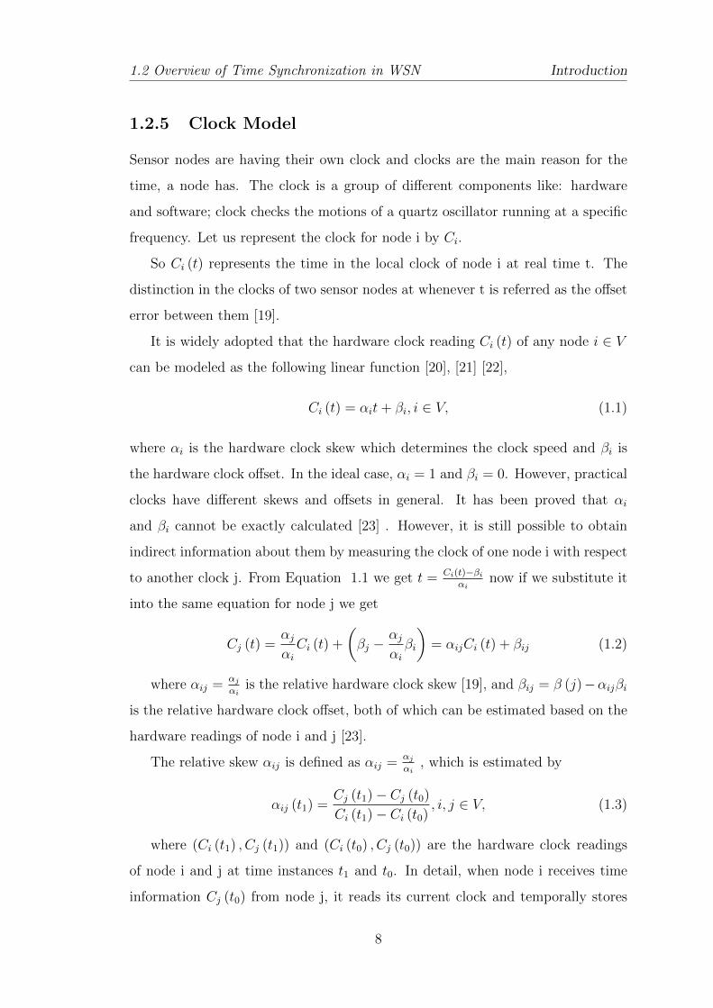
1.2.5 Clock Model
Sensor nodes are having their own clock and clocks are the main reason for the
time, a node has. The clock is a group of different components like: hardware
and software; clock checks the motions of a quartz oscillator running at a specific
frequency. Let us represent the clock for node i by Ci.
So Ci (t) represents the time in the local clock of node i at real time t. The
distinction in the clocks of two sensor nodes at whenever t is referred as the offset
error between them [19].
It is widely adopted that the hardware clock reading Ci (t) of any node i ∈ V
can be modeled as the following linear function [20], [21] [22],
Ci (t) = αit+ βi, i ∈ V, (1.1)
where αi is the hardware clock skew which determines the clock speed and βi is
the hardware clock offset. In the ideal case, αi = 1 and βi = 0. However, practical
clocks have different skews and offsets in general. It has been proved that αi
and βi cannot be exactly calculated [23] . However, it is still possible to obtain
indirect information about them by measuring the clock of one node i with respect
to another clock j. From Equation 1.1 we get t = Ci(t)−βiαi
now if we substitute it
into the same equation for node j we get
Cj (t) =αjαiCi (t) +
(βj −
αjαiβi
)= αijCi (t) + βij (1.2)
where αij =αj
αiis the relative hardware clock skew [19], and βij = β (j)−αijβi
is the relative hardware clock offset, both of which can be estimated based on the
hardware readings of node i and j [23].
The relative skew αij is defined as αij =αj
αi, which is estimated by
αij (t1) =Cj (t1)− Cj (t0)
Ci (t1)− Ci (t0), i, j ∈ V, (1.3)
where (Ci (t1) , Cj (t1)) and (Ci (t0) , Cj (t0)) are the hardware clock readings
of node i and j at time instances t1 and t0. In detail, when node i receives time
information Cj (t0) from node j, it reads its current clock and temporally stores
8

1.2 Overview of Time Synchronization in WSN Introduction
(Ci (t0) , Cj (t0)), and when node i receives the time information Cj (t1) from node
j for the second time, the relative skew αij can be obtained from equation 1.3
directly. After obtaining relative skew αji the relative hardware clock offset βji
can be obtained from equation 1.2 immediately βji = Ci (t)− αjiCj (t).
But this is not possible to update it manually [24] so we can define logical clock
Li (t) to replace hardware clock as follows,
Li (t) = αi (t)Ci (t) + βi (t)
and here we can put value of Ci (t) from equation 1.1 and get,
Li (t) = αi (t)αit+ αi (t) βi + βi (t)
Where αi (t) and βi (t) are two adjusting parameters, which are used for time
synchronization.
1.2.6 Attack Model
Time synchronization in wireless sensor networks is vulnerable to many security
attacks like sybil attack, replay attacks, message manipulation attack, delay attack
and Dos attack, etc., Here we will only focus on message manipulation attack,
which is defined as follows.
Message manipulation: It includes dropping and transmitting fake synchro-
nization messages. For instance, an attacker pretends as a safe node and corrupts
the synchronization information, e.g., hardware clock reading and adjusting pa-
rameters, and broadcasts to its neighbor nodes. In this way, the attack nodes can
mislead their neighbor nodes and damage the synchronization [25], [26] [27].
From the definition of Message manipulation, it follows that the replay attack,
delay attack and fault data injection attack can also be viewed as the different
kinds of message manipulation. For example, replay attack can be modeled as
adding a negative time to the real message, while delay attack can be viewed as
adding a delay to the real message. Since we focus on the maximum consensus
based time synchronization, the information for nodes communication includes
hardware clock readings and adjusting parameters. Thus, we assume that the
attackers has the ability to freely manipulate and broadcast the fake hardware
clock readings and adjusting parameters if they decide to attack.
9

Chapter 2
Literature review
Many time synchronization protocols have been proposed in the past few years,
e.g., RBS [28] [29] [30], TPSN [31], FTSP [32] [33] [34] [35] [36], etc. However,
most of these protocols are root-based or tree-based time synchronization pro-
tocols, which are sensitive to the dynamic network topology. Thus, in order
to enhance the robustness and scalability of the protocols, consensus concept,
e.g., average consensus, has been introduced to solve the time synchronization
problem in WSNs recently, which is called consensus-based time synchroniza-
tion [20] [37] [38] [39] [40] [41] [42] [43]. Compared with the traditional root-based
or tree-based time synchronization protocols, consensus-based time synchroniza-
tion protocols are fully distributed without requiring any certain reference node.
Meanwhile, the consensus-based time synchronization protocols are able to simul-
taneously compensate both the clock offset, i.e., instantaneous clock difference,
and the clock skew, i.e., clock speed, which can prolong there-synchronization pe-
riod and thus reducing communication and energy costs. The existing consensus-
based time synchronization protocols can be divided into two categories, i.e., av-
erage consensus-based [37] [21] and maximum consensus-based [20].
In RBS [28] [29] [30], at first sender node broadcast reference message and then
receiver node record their local time when they received a reference broadcast.
After that, they exchange the recorded time with each other.
J. Elson et al., in [28] proposed RBS protocol in which sender nodes send
reference signals to their neighbors utilizing physical-layer broadcasts. A reference
broadcasts does not contain an express timestamp; rather, beneficiaries utilize its
10

Literature review
entry time as a perspective for looking at their clocks. They utilize estimations
from two wireless used to show that expelling the sender’s nondeterminism from
the critical path in this way result in a dramatic improvement in synchronization
over using NTP, their protocol permits time to be proliferated crosswise over
broadcast domains without losing the reference-broadcast property. Their protocol
keeps up microsecond-level synchronization to an external timescale, for example,
UTC. As NTP protocol is not suited for energy use, precision, cost, scope, and
lifetime. Elson et al., in [29] proposed some configuration standard use numerous,
tunable modes of synchronization; don’t keep up a global timescale for the whole
network; use post-facto synchronization; adjust to the application, and exploit
domain knowledge.
F. Ren et al., proposed a new time synchronization protocol called Self-Correcting
Time Synchronization (SCTS). This protocol converts the time synchronization
problem into an online dynamic self-adjusting optimizing process. This conversion
is done to make offset and drift compensation simultaneously. The SCTS protocol
proposed by [30] completely misuses the inherent broadcast property of wireless
channel, so the communication overhead is noticeably low. They also proposed
equivalent digital PLL without a real voltage controlled oscillator to evade the
additional hardware needed by a traditional PLL circuit.
The main advantage of RBS is that it removes nondeterminism of transmitter
side, by using the idea of a time critical path. Time critical path contributes
to nondeterministic synchronization errors. The disadvantage of RBS is that it
requires a lot of extra message exchange to communicate the neighborhood times-
tamps between the nodes.
TPSN [31] is specially designed for wireless sensor network by doing some
modification in existing time synchronization protocol NTP which consist of two
phase in the first phase, a hierarchical structure is established in the network and
in second phase a pair wise synchronization is performed to establish a global
timescale throughout the network.
M. Maroti et al., uses low communication bandwidth for Flooding Time Syn-
11

Literature review
chronization Protocol [32]. Their protocol is robust in contrast to link and node
failure. They achieve robustness by exploiting periodic flooding of synchroniza-
tion messages and implicit dynamic topology update. They also use MAC-layer
timestamping by which he achieves high precision performance. In their protocol
average per-hop synchronization error is in the range of one microsecond. L. Ghe-
orghe et al., extends the Flooding Time Synchronization Protocol [33] by adding
fault-tolerance features. In their protocol if a node detects an inconsistence be-
tween the time received before and the time received at the moment, then their
protocol starts a decision process. For decision process they uses three steps: fault
detection, asking for help, and receiving help and decision. After these steps if
node determines the received information is faulty or not if the information is not
faulty then it is stored and if information is faulty then a new value is computed
from the time values received from the neighbors. Their algorithm detects faults
determined by malicious nodes or by transmission errors.
F. Ferrari et al., proposed Glossy, a flooding architecture [35] for WSNs that
takes the advantage of interference, by making concurrent transmissions of the
same packet interfere constructively. Even in the absence of capture effects, glossy
enables receivers to decode a packet. Glossy provides exact time synchronization
along with quick and exceptionally dependable flooding at ultra-low duty cycles.
In their protocol nodes gets the flooding packet with a probability higher than
99.99 %, while having its radio turned on for just a couple of milliseconds during
a flood.
D.-J. Huang et al., investigate the security vulnerability in Flooding Time Syn-
chronization Protocol [34] and they proposes several techniques to defend against
attacks from malicious nodes. They proposed a reference node selecting mecha-
nism to reduce the effect of multiple reference nodes, and proposed four filters to
defend against seqNum attack, global time attack, and node replication attack.
Y. Sinan et al., proposed Time Synchronization Based on Slow-Flooding in
Wireless Sensor Networks [36]. In FTSP it has been shown that slow-flooding de-
creases the synchronization accuracy and scalability. Alternatively, rapid-flooding
12

Literature review
approach allows nodes to propagate time information as quickly as possible . How-
ever, rapid flooding is difficult and has several drawbacks in wireless sensor net-
works. They tries to reduce the undesired effect of slow-flooding on the synchro-
nization accuracy without changing the propagation speed of the flood and for
that he proposed clock speed agreement algorithm.
FTSP is robust against node and link failures and it uses low communica-
tion bandwidth. For robustness it utilizes implicit dynamic topology update and
periodic flooding of synchronization messages. It uses linear regression for com-
pensating for clock skew to achieve accuracy.
TPSN [31], RBS [28] and FTSP [32] are type of centralized time synchroniza-
tion protocol and the convergence speed of the centralized time synchronization
protocol is usually fast and it has also little synchronization error, but in this type
of protocol we need a physical node which acting as the whole network reference
clock and in this type of protocol if reference node is out of work, then the protocol
will undergo from huge damage. One more disadvantage of the centralized time
synchronization protocol is that synchronization error rises with the increase of
network hops.
In Time Diffusion Synchronization Protocol [19] by using election/reelection
procedure periodically nodes self-determines to become master/diffusion leader,
and then master node broadcast timing information and after that timing infor-
mation is rebroadcasted by the diffused leader nodes and it forms a radial tree
structure. This approach is fully distributed, but it only compensates for clock
offset and not for clock skew and for this reason we have to increase the frequency
of synchronization.
In GSC [44] each node broadcast a synchronization request to their neighbor
and then neighbor respond with a message which contains local time. After re-
ceiving node averages the received timestamps and broadcasts this value back to
its neighbors which adopts this value as their new time. This is repeated by each
node until the whole network is synchronized. This approach is fully distributed,
but it also has the same problem that it only compensate for clock offset and not
13

Literature review
for clock skew.
L. Schenato et al., in [41] proposed a consensus-based protocol, referred as the
Average TimeSync main idea of his protocol is averaging local information. Their
protocol is computationally lite as it involves only simple sum/product operations,
fully distributed and, robust to node failure.
L. Schenato et al., in [37] proposed Average TimeSync protocol whose main
idea is to average local information to achieve a global agreement on a specific
quantity of interest. Their proposed algorithm is computationally light, robust
to dynamic network topologies due, asynchronous, fully distributed and includes
drift compensation.
J. He et al., in [39] investigate the impact of message manipulation attacks
over ATS and proposed a novel secured maximum consensus based time synchro-
nization protocol to defend against message manipulation attacks.
J. He et al., propose Maximum Consensus based time synchronization protocol
[20]. The main idea of Maximum Value Based Consensus Approach is to maximize
the local information to achieve a global synchronization. The proposed approach
has faster convergence speed and compensate both clock skew and clock offset
simultaneously. The proposed protocol is asynchronous, robust against packet
losses, nodes failure and the addition of new nodes and completely distributed.
J. He et al., in [38] investigate the impact of message manipulation attacks
over MTS and proposed a novel secured maximum consensus based time synchro-
nization protocol to defend against message manipulation attacks.
X. Yongjun, in [43] proposes Max and Average Consensus based time synchro-
nization protocol for WSNs, which uses max consensus to compensate for clock
drift and average consensus to compensate for clock offset. The main idea of their
protocol is to achieve a global synchronization by just using local information.
Their protocol has the advantage of being asynchronous, totally distributed and
robust to packet drop and sensor node failure. They reduces the clock error to 10
ticks.
J. He et al., in [40] investigates consensus-based time synchronization protocols
14

Literature review
in practical sensor networks through extensive testbed experiments. They analyze
how the time synchronization accuracy will be affected by various uncertainties in
the system and they also investigate the time synchronization performance and
robustness under various network settings and find MTS is slightly faster than the
desirable clock, by adopting both maximum consensus and minimum consensus,
they propose a modified protocol, MMTS, which is able to drive the synchronized
clocks closer to the desirable clock while maintaining the convergence rate and
synchronization accuracy of MTS.
15

Chapter 3
Maximum and MinimumConsensus based TimeSynchronization
In this chapter, we give a brief idea of working of MMTS protocol and investigate
MMTS protocol over message manipulation attack.
In MMTS [40], each node i broadcasts its current hardware clock reading Ci (t),
the current skew compensation αi and offset compensation βi and µi and νi to its
neighbor nodes. However, it is not assumed that the message is guaranteed to be
received each time. When the nodes receive these messages from their neighboring
nodes, they will adjust their logical clocks accordingly. Eventually, by the iteration
of the algorithm, the logical clock skew of all nodes will equal to the average of
maximum hardware clock skew & minimum hardware clock skew and logical clock
offset of all nodes will equal to average of maximum hardware clock offset &
minimum hardware clock offset.
� Set initial condition as αi = 1, βi = 0, µi = 0 and νi = 0 for each node i and
for each its neighbor.
� Each node i broadcast its local hardware clock reading Ci (t) , αi, βi, µi and
νi to its neighbors.
� If node i receive the packet from node j at time tk, k ∈{
0, N+
}, then records
its current hardware clock reading and calculate αij (k) by
αij (k) =Cj(k)−Cj(k−1)
Ci(k)−Ci(k−1)+(k−1)αij(k−1)
k
16

Maximum and Minimum Consensus based Time Synchronization
when k is greater than or equal to one.
� Compute αimax, βimax, αimin and βimin respectively by
αimax = αi + µi
βimax = βi + νi
αimin = αi − µi
βimin = βi − νi
then, compute
Pij (k) =αij(k)(αj+µj)
αimaxand Qij (k) =
αij(k)(αj−µj)αimin
� Maximum consensus: If Pij (k) > 1, then
αimax = αij (k) (αj + µj) and
βimax = (αj + µj)Cj (tk) + βj + νj − αij (k) (αj + µj)Ci (tk)
if Pij (k) = 1, then
βimax = maxl=i,j
{(αl + µl)Cl (tk) + βl + νl
}− (αi + µi)Ci (tk)
� Minimum consensus: If Qij (k) < 1, then
αimin = αij (k) (αj − µj) and
βimin = (αj − µj)Cj (tk) + βj − νj − αij (k) (αj − µj)Ci (tk)
if Qij (k) = 1, then
βimin = minl=i,j
{(αl − µl)Cl (tk) + βl − νl
}− (αi − µi)Ci (tk)
� Update parameters αi, βi, µi and νi respectively by
αi = αimax+αimin
2
βi = βimax+βimin
2
µi = αimax−αimin
2
νi = βimax−βimin
2
� Replace[Ci (tk−1) , Cj (tk−1) , αij (k − 1)
]by[Ci (tk) , Cj (tk) , αij (k)
]17

3.1 MMTS under attackMaximum and Minimum Consensus based Time Synchronization
3.1 MMTS under attack
From MMTS algorithm, it can be observed that for maximum consensus node i
will select its neighbor node j as the reference node when node j has larger logical
clock skew or has the same logical clock skew, but a larger logical clock and for
minimum consensus node i will select its neighbor node j as the reference node
when node j has smaller logical clock skew or has the same logical clock skew but
smaller logical clock.
The attacker may manipulate the message in a random way to destroy the time
synchronization. For example, let node j be the attack node, which broadcasts
fake messages with hardware clock reading Cej (tk) and logical clock adjusting
parameters αej (tk) , βej (tk) , µej (tk) and νej (tk) where values of these fake messages
can be arbitrarily chosen by node j. thus, when a safe node i receives such fake
message Cej from node j, it will estimate the relative skew according to
αeij (t1) =Ce
j (t1)−Cej (t0)
Ci(t1)−Ci(t0)
αeij (t1) =Ce
j (t1)−Cej (t0)
Cj(t1)−Cj(t0)
Cj(t1)−Cj(t0)
Ci(t1)−Ci(t0)
αeij (t1) = δej (t1)αij
where δej (t1) =Ce
j (t1)−Cej (t0)
Cj(t1)−Cj(t0)is the value of the fake hardware clock distance
over the true distance between two consecutive communication times, since the
node j is able to change the value of Cej (t) freely, it can determine δej (t). Since
value of αij needed for both skew compensation and offset compensation so it
affects both values.
18

Chapter 4
Secure Maximum and MinimumConsensus based TimeSynchronization
In this chapter we will provide the details of secured MMTS (SMMTS). The overall
architecture of SMMTS is depicted in Fig. 4.1, which consists of six components.
Since message reception and verification, message generation and authentication,
message broadcasting are common components for different protocols.
Figure 4.1: Overall architecture of SMMTS
19

4.1 Hardware clock checking process:Secure Maximum and Minimum Consensus based Time Synchronization
4.1 Hardware clock checking process:
The hardware clock checking process, i.e., safeguard mechanism of hardware clock,
is introduced as follows.
for all i, j ∈ ν, define Sij (k) as one step relative skew estimation for node i
with respect to node j,
Sij (k) =Cj(tk)−Cj(tk−1)
Ci(tk)−Ci(tk−1)
where k denotes k-th of estimation, tk is the corresponding real time. The
following distributed algorithm RSE is used to estimate the relative skew of each
neighbor pair of nodes.
� Set ε1 ≥ 0 to each node i, i ∈ ν.
� Each node i broadcasts its current hardware clock reading Ci (t) to its neigh-
bor nodes at each iteration.
� For any node i’s neighbor node, say node j, upon receiving a message from
node i, it records (Ci (t) , Cj (t)).
� If node j successfully receives message from node i more than once, it then
compute Sij (k) by above equation.
� For all K > 1, if Sij (k) satisfies∣∣∣Sij (k)− Sij (1)
∣∣∣ ≤ ε1 for all i ∈ Nj then node j assign αij (k) = Sij (k)
otherwise, it will deem node i as the attack node, and break up with node i
by ignoring all its following messages.
The above algorithm utilizes the linear clock model to check the consecutive
neighbor hardware readings at each time step, so that the attacker, if exists, cannot
freely change the hardware clock reading for broadcasting.
4.2 Logical Clock checking process:
Here we describes the logical clock checking process, i.e., safeguard mechanism of
logical clock.
20

4.2 Logical Clock checking process:Secure Maximum and Minimum Consensus based Time Synchronization
Note that if a node j selects node is logical clock as the reference clock, the αj
and βj used for the updates of node j should satisfy respectively
αj =αiαij
(4.1)
and
βj = αiCi (t0) + βi − αjCj (t0) (4.2)
where Ci (t0) and Cj (t0) are obtained from RSE algorithm. Thus node i can
calculate αj and βj respectively by using 4.1 and 4.2 based on the information
held by itself. This fact is exploited to develop the logical clock checking process
for SMMTS. Before broadcasting, each node will authenticate the information so
that all its neighbors can only read. Specifically, with the localized encryption and
authentication protocol, each node will only share the reading key, which prevents
neighbor nodes to manipulate the message.
Before presenting the details of logical clock checking process, we would like to
first briefly define the communication format among sensor nodes. Define λ∗ij =
[λ∗ij (1) , λ∗ij (2) , λ∗ij (3) , λ∗ij (4)] as the authenticated message which is created by
node i and used for broadcasting to its neighbor node j, where λ∗ij (1) = αj,
λ∗ij (2) = βj, λ∗ij (3) = µi and λ∗ij (4) = νi. In order to run the logical clock checking
process, let the packet for node i broadcasting should include λ∗ij and λ∗li, where λ∗li
is the message received from a neighbor node l by node i, and λ∗li (1) , λ∗li (2) , λ∗li (3)
and λ∗li (4) are respectively equal to the current adjusting parameters used for the
node is logical clock. If node i has not yet updated its logical clock based on λ∗li
for all l ∈ Ni and l 6= i, let λ∗li = λ∗ii = [1, 0, 0, 0] and use λ∗ii for broadcasting, i.e.,
λ∗li = [1, 0, 0, 0] for l = i.
Now, the key step of logical clock checking process is provided, which prevents
the attack node i from freely using incorrect αi, βi, µi and νi to attack. That is,
when node j receives the information from node i and selects node is logical clock
as the reference clock, it checks whether the following two equations hold true or
not.
21

4.3 SMMTS ProtocolSecure Maximum and Minimum Consensus based Time Synchronization
∣∣∣λ∗ij (1) + λ∗ij (3)− (λ∗li (1) + λ∗li (3))αji
∣∣∣ ≤ ε2 (4.3)
where ε2 ≥ 0, and
X = λ∗ij (2) + λ∗ij (4) + Cj (t1)(λ∗ij (1) + λ∗ij (3)
)Y = λ∗li (2) + λ∗li (4) + Ci (t1)
(λ∗ij (1) + λ∗ij (3)
)∣∣∣X − Y ∣∣∣ ≤ ε3 (4.4)
where ε3 ≥ 0.
The logical clock checking process guarantees that node j updates it logical
clock based on correct λ∗ij, which is received and created by the neighbor node
i. Therefore, logical clock checking process designed for SMMTS ensures that all
safe nodes will not use incorrect adjusting parameters for clock updates.
4.3 SMMTS Protocol
In SMMTS, after the received messages pass the hardware clock and logical clock
checking processes, the nodes will update their logical clock based on MMTS. The
details of SMMTS are introduced as follows.
� Set initial condition as αi = 1, βi = 0, µi = 0 and νi = 0 for each node i and
for each its neighbor.
� Apply RSE to estimate the relative skews for each node and its neighbor
nodes.
� At each iteration, node i computes Qij and pij by pij (t) =αij(t)(αj+µj)
αi+µiand
Qij (t) =αij(t)(αj−µj)
αi−µi .
� Create λ∗ij.
� Broadcast λ∗li and λ∗ij to node j.
� If both 4.3 and 4.4 are true,
αj = λ∗ij (1) , βj = λ∗ij (2) , µj = λ∗ij (3) and νj = λ∗ij (4).
22

4.3 SMMTS ProtocolSecure Maximum and Minimum Consensus based Time Synchronization
Then, node j stores λ∗ij and αi = λ∗li (1).
� If both 4.3 and 4.4 or one of them is false, then node j will regard node i as
an attack node and will no longer use the information received from node i
for logical clock updates.
23

Chapter 5
Simulation and results
5.1 MMTS
For simulation of MMTS, we set αi (0) = 1, βi (0) = 0, µi = 0 and νi = 0 and let
each skew αi of the hardware clock be randomly selected from the interval 0.8 to
1.2 and offset βi of node i be randomly selected from the interval 0 to 0.4. For
each iteration k, let ds is variable, which is measured by the maximum difference
of the logical clock skew of all nodes.
Figure 5.1: Performance of MMTS under attack
24

5.1 MMTS Simulation and results
In order to show the performance of MMTS under message manipulation, we
conduct simulation on a network with 30 nodes. Suppose at the first stage, all the
nodes behave exactly according to the MMTS protocol. But when we compromised
one node. Suppose node 10 is compromised by the attacker and will broadcast
α10 + ω10 to its neighbor nodes. Let ds (t) be the maximum difference between
the logical skews of any two safe nodes, Fig 5.1 shows the trajectories of ds (t).
It can be observed that ds will finally vary over an average value of around 0.1,
which further indicates that the maximal logical clock difference would diverge in
a approximately linear speed with a high probability. Apparently, a single node
attack can deteriorate the performance of MMTS in an easy way.
25

5.2 SMMTS Simulation and results
5.2 SMMTS
For simulation of SMMTS, we set αi (0) = 1, βi (0) = 0, µi = 0 and νi = 0 and let
each skew αi of the hardware clock be randomly selected from the interval 0.8 to
1.2 and offset βi of node i be randomly selected from the interval 0 to 0.4. For each
iteration k, let dmax is variable, which is measured by the maximum difference of
the logical clock skew of safe nodes.
Figure 5.2: Performance of SMMTS under attack
From Fig 5.2 we see that at starting value of ds is about 0.37 this is because
for simulation we randomly select value of hardaware clock skew between 0.8 to
1.2, and we see that value of ds for SMMTS is become 0 after about 200 broadcast
that means all safe nodes logical clock running at same rate after 200 broadcast.
26

Chapter 6
Conclusions and future work
This thesis investigates time synchronization under cyber physical attacks in WSNs.
By theoretical analysis and simulation results it is clear that existing Maximum
and Minimum consensus based Time Synchronization (MMTS) protocol is invalid
under message manipulation attacks defined in this thesis. A Secured Maximum
and Minimum consensus based Time Synchronization (SMMTS) protocol is pro-
posed to defend against message manipulation attacks. Specifically, in SMMTS,
by carefully designing the hardware clock and logical clock checking processes, it
will be able to detect and invalidate the potential message manipulation attacks.
Meanwhile, the maximum and minimum consensus based logical clock updating
process guarantees faster convergence and compensates clock skew and offset si-
multaneously and logical clock does not deviate more from real clock. In future
we can investigate more attack on Time Synchronization Algorithm and proposed
proper solution for that attack.
27

Bibliography
[1] I. F. Akyildiz, W. Su, Y. Sankarasubramaniam, and E. Cayirci, “Wireless
sensor networks: a survey,” Computer networks, vol. 38, no. 4, pp. 393–422,
2002.
[2] A. Chandrakasan, R. Amirtharajah, S. Cho, J. Goodman, G. Konduri, J. Ku-
lik, W. Rabiner, and A. Wang, “Design considerations for distributed mi-
crosensor systems,” in Custom Integrated Circuits, 1999. Proceedings of the
IEEE 1999, pp. 279–286, IEEE, 1999.
[3] P. Bonnet, J. Gehrke, and P. Seshadri, “Querying the physical world,” Per-
sonal Communications, IEEE, vol. 7, no. 5, pp. 10–15, 2000.
[4] M. Castillo-Effer, D. H. Quintela, W. Moreno, R. Jordan, and W. Westhoff,
“Wireless sensor networks for flash-flood alerting,” in Devices, Circuits and
Systems, 2004. Proceedings of the Fifth IEEE International Caracas Confer-
ence on, vol. 1, pp. 142–146, IEEE, 2004.
[5] A. Mainwaring, D. Culler, J. Polastre, R. Szewczyk, and J. Anderson, “Wire-
less sensor networks for habitat monitoring,” in Proceedings of the 1st ACM
international workshop on Wireless sensor networks and applications, pp. 88–
97, ACM, 2002.
[6] X. Yu, N. Venkatasubramanian, K. Niyogi, and S. Mehrotra, “Adaptive mid-
dleware for distributed sensor environments,” IEEE Distributed Systems On-
line, vol. 4, no. 5, 2003.
[7] W. Yuan, S. V. Krishnamurthy, and S. K. Tripathi, “Synchronization of mul-
tiple levels of data fusion in wireless sensor networks,” in Global Telecom-
28

BIBLIOGRAPHY BIBLIOGRAPHY
munications Conference, 2003. GLOBECOM’03. IEEE, vol. 1, pp. 221–225,
IEEE, 2003.
[8] J. Zhao, R. Govindan, and D. Estrin, “Computing aggregates for monitor-
ing wireless sensor networks,” in Sensor Network Protocols and Applications,
2003. Proceedings of the First IEEE. 2003 IEEE International Workshop on,
pp. 139–148, IEEE, 2003.
[9] K. Christos, “Time synchronization in wireless sensor networks,” University
of Patras, 2009.
[10] K. Daniluk, “Time synchronization in wireless sensor networks,”
[11] A. E. Khandani, E. Modiano, J. Abounadi, and L. Zheng, “Cooperative rout-
ing in wireless networks,” in Advances in Pervasive Computing and Network-
ing, pp. 97–117, Springer, 2005.
[12] A. Woo and D. E. Culler, “A transmission control scheme for media access in
sensor networks,” in Proceedings of the 7th annual international conference
on Mobile computing and networking, pp. 221–235, ACM, 2001.
[13] L. Girod and D. Estrin, “Robust range estimation using acoustic and multi-
modal sensing,” in Intelligent Robots and Systems, 2001. Proceedings. 2001
IEEE/RSJ International Conference on, vol. 3, pp. 1312–1320, IEEE, 2001.
[14] F. Sivrikaya and B. Yener, “Time synchronization in sensor networks: a sur-
vey,” Network, IEEE, vol. 18, no. 4, pp. 45–50, 2004.
[15] J. Bae and B. Moon, “Time synchronization in wireless sensor networks,”
[16] R. Fengyuan, “Time synchronization in wireless sensor networks,” 2005.
[17] G. C. Gautam, T. Sharma, V. Katiyar, and A. Kumar, “Time synchronization
protocol for wireless sensor networks using clustering,” in Recent Trends in In-
formation Technology (ICRTIT), 2011 International Conference on, pp. 417–
422, IEEE, 2011.
29

BIBLIOGRAPHY BIBLIOGRAPHY
[18] S. Ganeriwal, C. Popper, S. Capkun, and M. B. Srivastava, “Secure time
synchronization in sensor networks,” ACM Transactions on Information and
System Security (TISSEC), vol. 11, no. 4, p. 23, 2008.
[19] W. Su and I. F. Akyildiz, “Time-diffusion synchronization protocol for wire-
less sensor networks,” Networking, IEEE/ACM Transactions on, vol. 13,
no. 2, pp. 384–397, 2005.
[20] J. He, P. Cheng, L. Shi, and J. Chen, “Time synchronization in wsns: A
maximum value based consensus approach,” in Decision and Control and
European Control Conference (CDC-ECC), 2011 50th IEEE Conference on,
pp. 7882–7887, IEEE, 2011.
[21] L. Schenato and F. Fiorentin, “Average timesync: A consensus-based proto-
col for time synchronization in wireless sensor networks,” in Estimation and
Control of Networked Systems, vol. 1, pp. 30–35, 2009.
[22] P. Sommer and R. Wattenhofer, “Gradient clock synchronization in wire-
less sensor networks,” in Proceedings of the 2009 International Conference
on Information Processing in Sensor Networks, pp. 37–48, IEEE Computer
Society, 2009.
[23] G. Werner-Allen, G. Tewari, A. Patel, M. Welsh, and R. Nagpal, “Firefly-
inspired sensor network synchronicity with realistic radio effects,” in Pro-
ceedings of the 3rd international conference on Embedded networked sensor
systems, pp. 142–153, ACM, 2005.
[24] D. Zhou and T.-H. Lai, “An accurate and scalable clock synchronization
protocol for ieee 802.11-based multihop ad hoc networks,” Parallel and Dis-
tributed Systems, IEEE Transactions on, vol. 18, no. 12, pp. 1797–1808, 2007.
[25] Q. Yan, M. Li, T. Jiang, W. Lou, and Y. T. Hou, “Vulnerability and pro-
tection for distributed consensus-based spectrum sensing in cognitive radio
networks,” in INFOCOM, 2012 Proceedings IEEE, pp. 900–908, IEEE, 2012.
30

BIBLIOGRAPHY BIBLIOGRAPHY
[26] R. Lu, X. Lin, H. Zhu, X. Liang, and X. Shen, “Becan: a bandwidth-efficient
cooperative authentication scheme for filtering injected false data in wireless
sensor networks,” Parallel and Distributed Systems, IEEE Transactions on,
vol. 23, no. 1, pp. 32–43, 2012.
[27] X. Hu, T. Park, and K. G. Shin, “Attack-tolerant time-synchronization in
wireless sensor networks,” in INFOCOM 2008. The 27th Conference on Com-
puter Communications. IEEE, IEEE, 2008.
[28] J. Elson, L. Girod, and D. Estrin, “Fine-grained network time synchroniza-
tion using reference broadcasts,” ACM SIGOPS Operating Systems Review,
vol. 36, no. SI, pp. 147–163, 2002.
[29] J. Elson and K. Romer, “Wireless sensor networks: A new regime for time syn-
chronization,” ACM SIGCOMM Computer Communication Review, vol. 33,
no. 1, pp. 149–154, 2003.
[30] F. Ren, C. Lin, and F. Liu, “Self-correcting time synchronization using refer-
ence broadcast in wireless sensor network,” Wireless Communications, IEEE,
vol. 15, no. 4, pp. 79–85, 2008.
[31] S. Ganeriwal, R. Kumar, and M. B. Srivastava, “Timing-sync protocol for
sensor networks,” in Proceedings of the 1st international conference on Em-
bedded networked sensor systems, pp. 138–149, ACM, 2003.
[32] M. Maroti, B. Kusy, G. Simon, and A. Ledeczi, “The flooding time syn-
chronization protocol,” in Proceedings of the 2nd international conference on
Embedded networked sensor systems, pp. 39–49, ACM, 2004.
[33] L. Gheorghe, R. Rughinis, and N. Tapus, “Fault-tolerant flooding time syn-
chronization protocol for wireless sensor networks,” in Networking and Ser-
vices (ICNS), 2010 Sixth International Conference on, pp. 143–149, IEEE,
2010.
31

BIBLIOGRAPHY BIBLIOGRAPHY
[34] D.-J. Huang, K.-J. You, and W.-C. Teng, “Secured flooding time synchroniza-
tion protocol,” in Mobile Adhoc and Sensor Systems (MASS), 2011 IEEE 8th
International Conference on, pp. 620–625, IEEE, 2011.
[35] F. Ferrari, M. Zimmerling, L. Thiele, and O. Saukh, “Efficient network flood-
ing and time synchronization with glossy,” in Information Processing in Sen-
sor Networks (IPSN), 2011 10th International Conference on, pp. 73–84,
IEEE, 2011.
[36] Y. Sinan et al., “Time synchronization based on slow flooding in wireless
sensor networks,” 2013.
[37] L. Schenato and F. Fiorentin, “Average timesynch: A consensus-based proto-
col for clock synchronization in wireless sensor networks,” Automatica, vol. 47,
no. 9, pp. 1878–1886, 2011.
[38] J. He, J. Chen, P. Chen, and X. Cao, “Secure time synchronization in wireless
sensor networks: A maximum consensus based approach,” 2013.
[39] J. He, P. Cheng, L. Shi, and J. Chen, “Sats: Secure average-consensus-based
time synchronization in wireless sensor networks,” 2013.
[40] J. He, H. Li, J. Chen, and P. Cheng, “Study of consensus-based time syn-
chronization in wireless sensor networks,” ISA transactions, 2013.
[41] L. Schenato and G. Gamba, “A distributed consensus protocol for clock syn-
chronization in wireless sensor network,” in Decision and Control, 2007 46th
IEEE Conference on, pp. 2289–2294, IEEE, 2007.
[42] W. Ren, R. W. Beard, and E. M. Atkins, “A survey of consensus problems in
multi-agent coordination,” in American Control Conference, 2005. Proceed-
ings of the 2005, pp. 1859–1864, IEEE, 2005.
[43] X. Yongjun, “Time synchronization in wireless sensor networks using max
and average consensus protocol,” International Journal of Distributed Sensor
Networks, vol. 2013, 2013.
32

BIBLIOGRAPHY BIBLIOGRAPHY
[44] Q. Li and D. Rus, “Global clock synchronization in sensor networks,” Com-
puters, IEEE Transactions on, vol. 55, no. 2, pp. 214–226, 2006.
33