Time-SeriesAnalysis andCyclostratigraphycatdir.loc.gov/catdir/samples/cam033/2002067374.pdf ·...

Time-Series Analysisand CyclostratigraphyExamining stratigraphic recordsof environmental cycles

Graham P. Weedon

published by the press syndicate of the university of cambridgeThe Pitt Building, Trumpington Street, Cambridge, United Kingdom

cambridge university pressThe Edinburgh Building, Cambridge CB2 2RU, UK40 West 20th Street, New York, NY 10011-4211, USA477 Williamstown Road, Port Melbourne, VIC 3207, AustraliaRuiz de Alarcon 13, 28014 Madrid, SpainDock House, The Waterfront, Cape Town 8001, South Africa

http://www.cambridge.org

C© Cambridge University Press 2003

This book is in copyright. Subject to statutory exceptionand to the provisions of relevant collective licensing agreements,no reproduction of any part may take place withoutthe written permission of Cambridge University Press.

First published 2003

Printed in the United Kingdom at the University Press, Cambridge

TypefacesTimes 10.25/13.5 pt and Joanna SystemLATEX2ε [tb]

A catalogue record for this book is available from the British Library

Library of Congress Cataloguing in Publication data

Weedon, Graham P. (Graham Peter), 1962– .Times-series analysis and cyclostratigraphy: examining stratigraphic recordsof environmental cycles/Graham P. Weedon.

p. cm.Includes bibliographical references and index.ISBN 0 521 62001 51. Cyclostratigraphy. 2. Time-series analysis. I. Title.QE651.5. W44 2003551.7′01′51955–dc21 2002067374

The publisher has used its best endeavours to ensure that the URLs for externalwebsites referred to in this book are correct and active at the time of goingto press. However, the publisher has no responsibility for the website andcan make no guarantee that a site will remain live or that the content is orwill remain appropriate.

ISBN 0 521 62001 5 hardback

Contents

Preface xi

Acknowledgements xiii

Chapter 1 Introduction 1

1.1 Cyclostratigraphic data 1

1.2 Past studies of cyclicsediments 3

1.3 Time-series analysis – an introduction 6

1.4 Chapter overview 20

Chapter 2 Constructing time series in cyclostratigraphy 21

2.1 Introduction 21

2.2 Categories of cyclostratigraphic time series 22

2.2.1 Continuous-signal records 23

2.2.2 Discrete-signal records 26

2.2.2a Periodic discrete-signal records 27

2.2.2b Quasi-periodic discrete-signal records 27

2.2.2c Aperiodic discrete-signal records 27

2.3 Requirements for the generation of stratigraphic time series 28

2.3.1 Condition 1 – Consistent environmental conditions 28

2.3.2 Condition 2 – Unambiguous variable 28

2.3.3 Condition 3 – Thickness–time relationship 29

2.3.3a Continuous-signal records 29

2.3.3b Discrete-signal records 31

vii

viii Contents

2.4 Sampling 32

2.4.1 Sample intervals and power spectra 33

2.4.2 Sample intervals and aliasing 34

2.4.3 Missing values and irregular sample intervals 39


Chapter 3 Spectral estimation 43

3.1 Introduction 43

3.2 Processing of time series prior to spectral analysis 44

3.2.1 Mean subtraction 44

3.2.2 Ergodicity, stationarity and detrending 44

3.2.3 Outlier removal and the unit impulse 48

3.2.4 Pre-whitening 49

3.2.5 Other data transformations 52

3.3 Spectral estimation – preliminary considerations 55

3.3.1 Classes of spectra and noise models 55

3.3.2 Spectral resolution and bandwidth 58

3.3.3 Data tapering, spectral side-lobes and bias 61

3.3.4 Comparing spectra and normalization 63

3.4 Spectral estimation – methods 64

3.4.1 The Fourier transform and the periodogram 64

3.4.2 The direct method 69

3.4.3 The multi-taper method 70

3.4.4 The Blackman–Tukey method 75

3.4.5 The maximum entropy method 77

3.4.6 The Walsh method 79

3.5 The statistical significance of spectral peaks 81


Chapter 4 Additional methods of time-series analysis91

4.1 Introduction 91

4.2 Evolutionary spectra 91

4.3 Filtering 95

4.4 Complex demodulation 101

4.5 Cross-spectral analysis 103

4.5.1 Coherency spectra 103

4.5.2 Phase spectra 107

4.6 Wavelet analysis 112

4.7 Phase portraits and chaos 115

Contents ix

4.8 Singular spectrum analysis 123


Chapter 5 Practical considerations 129

5.1 Introduction 129

5.2 Cyclostratigraphic signal distortions related toaccumulation rate 130

5.2.1 Trends in accumulation rate 130

5.2.2 Random changes in accumulation rate 133

5.2.3 Abrupt or step changes in accumulation rate 135

5.2.4 Signal-driven accumulation rates, harmonics andcombination tones 135

5.3 Cyclostratigraphic signal distortions related to otherprocesses 142

5.3.1 Rectification 142

5.3.2 Bioturbation 144

5.3.3 Undetected hiatuses 145

5.4 Practical time-series analysis 149

5.4.1 How long should a time series be? 149

5.4.2 Interpreting spectral peaks 155


Chapter 6 Environmental cycles recorded stratigraphically 161

6.1 Introduction 161

6.2 The climatic spectrum 162

6.3 Tidal cycles 170

6.3.1 Tidal cycles and orbital dynamics 170

6.3.2 Stratigraphic records of tidal cycles 178

6.3.3 Records of tidal cycles and the Earth’s orbitalparameters 180

6.4 Annual cycles 181

6.5 The ElNino/SouthernOscillation 184

6.5.1 The El Nino/Southern Oscillation system 184

6.5.2 Stratigraphic records of ENSO variability 186

6.6 The North Atlantic Oscillation 187

6.7 Solar activity cycles 190

6.7.1 Sunspot cycles and solar physics 190

6.7.2 Stratigraphic records of solar cycles 194

6.8 Millennial-scale cycles and Heinrich events 195

x Contents

6.8.1 Latest Pleistocene Heinrich events and millennial-scale climaticcycles in the North Atlantic 195

6.8.2 Climatic mechanisms involved in North Atlantic millennial-scalecycles and Heinrich events 197

6.8.3 Evidence for millennial-scale cycles outside the NorthAtlantic region 198

6.8.4 Earlier records and the origin of millennial-scale cycles 199

6.9 Milankovitch cycles 200

6.9.1 The nature and climatic expression of the orbital cycles 200

6.9.1a Precession 204

6.9.1b Eccentricity 205

6.9.1c Obliquity 206

6.9.2 Earth’s orbital history 206

6.9.3 Orbital tuning 207

6.9.3a Tuning of Pliocene–Recent cyclostratigraphic records 207

6.9.3b Tuning of older cyclostratigraphic records 209

6.9.4 Stratigraphic records of Milankovitch cycles 212

6.9.4a Results from stratigraphic studies 212

6.9.4b The 100-ka cycles in the late Pleistocene 214


Appendix – published algorithms for time-series analysis 217

References 221

Index 252

Chapter 1

Introduction

1.1 Cyclostratigraphic data

Increasingly, quantitative records of environmental change covering intervals of be-tween half a day to millions of years are being sought by palaeoceanographers, en-vironmental scientists, palaeoclimatologists, sedimentologists and palaeontologists.The ‘media’ from which these records are obtained range from sediments and sedi-mentary rocks to living organisms and fossils showing growth bands (especially trees,corals and molluscs), ice cores and cave calcite. This book is concerned with explain-ing the quantitative methods that can be employed to derive useful information fromthese records. Much of the discussion is concerned with explaining the problems andlimitations of the procedures and with exploring some of the difficulties with interpre-tation. Most frequently environmental records are obtained from sedimentary sectionsmaking up the stratigraphic record and, using a rather broad definition, all the ‘media’described above are ‘stratigraphic’. The nature of cycles in environmental signals andin stratigraphic records are explored later. However, for now cycles can be thought ofas essentially periodic, or regular, oscillations in some variable. The study of strati-graphic records of environmental cycles has been called cyclostratigraphy (Fischeret al., 1990).

By regarding stratigraphic records of environmental changeas signals, it is clear thatthe methods and interpretations reached during analysis must allow for the imperfec-tions inherent in all recording procedures. In cyclostratigraphic data the environmentalsignal, which is ‘encoded’ during sedimentation, is often corrupted to some extent byinterruptions caused by processes that are not part of the normal depositional system.Such processes, for sediments, include non-deposition, erosion, seafloor dissolution orevent-bed deposition and they make the later recognition of the normal environmental

1

2 Introduction

signal more difficult. Yet the interruptions convey information themselves, and insome cases they result from the extremes of the normal environmental variations. Forexample, Dunbaret al. (1994), in their study of corals, pointed out that growth bandthickness was related to sea surface temperature. However, episodes of unusually highsea surface temperatures cause growth band generation to stop completely for severalyears, thus interrupting the proxy temperature record.

As well as interruptions, the recording processes can introduce distortions thatneed to be taken into account. For example, accumulation rate variations and diage-nesis frequently modify the final shapes of cyclostratigraphic data sets. In a similarmanner to the interruptions, the distorting processes often depend on the nature ofthe environment. Hence, cyclostratigraphic data contain information about normalenvironmental variability, abnormal environmental variations and the processes thatproduce the records themselves. In other words, the stratigraphic information that isobserved can be regarded as the product of many superimposed environmental andsedimentological, or metabolic, processes.

The methods described in this book are primarily concerned with detecting and de-scribing regular cyclic environmental processes. Hence, the data are treated as thoughthey consist of regular cycles plus irregular oscillations. The irregular componentsresult from both normal and abnormal environmental conditions as well as the effectsof sedimentation and diagenesis (or equivalent processes in skeletal growth, etc.). Asexplained below, there are sound geological reasons for using mathematics to searchfor regular cycles. Regular components of cyclostratigraphic data are often studiedmore easily than the irregular components. If methods could be developed to distin-guish the various types and origins of the irregular components, much of value couldbe uncovered. Quantitative studies of the interruption and distortion processes willundoubtedly be useful for understanding ancient environmental and diagenetic mech-anisms, but such investigations are relatively rare (e.g. Sadler, 1981; Ricken, 1986;Ricken and Eder, 1991; Ricken, 1993).

The idea that stratigraphic data consist of regular components – the signal, plusirregular components or noise – is based on a linear view of the processes involved.In reality non-linear processes abound in environmental systems (e.g. Le Treut andGhil, 1983; Imbrieet al., 1993a; Smith, 1994). In non-linear systems, the output doesnot vary in direct proportion to the input. There are many aspects of cyclostratigraphicdata that cannot be easily investigated using the standard linear methods of analysisdescribed in this book. From the perspective of non-linear dynamical systems, part ofthe irregular components can be considered to be as much a part of the environmentalsignal as the regular components (Stewart, 1990; Kantz and Schreiber, 1997). Somenon-linear methods are described very briefly within Chapter 4 and some non-linearissues in signal distortion are considered in Chapter 5. Despite the view that non-linear approaches might explain more of the data than the linear methods, the latterare currently best understood mathematically and are the most frequently used.

A good demonstration of the success of the standard linear approach to cyclostrati-graphic data concerns the timescale developedusing lateNeogenedeep-sea sediments.

1.2 Past studies of cyclic sediments 3

Hilgen (Hilgen and Langereis, 1989; Hilgen, 1991) and Shackletonet al.(1990) inde-pendently derived orbital cycle chronologies based on matching sedimentary cyclesand oxygen isotope curves to the calculated history of insolation changes (Section 6.9).The results were at odds with the widely accepted radiometric ages that had been ob-tained using potassium-argon dating. Subsequently, improved radiometric dating andstudies of sea-floor spreading rates confirmed the validity and utility of the so-calledastronomical time scale approach (Wilson, 1993; Shackletonet al., 1995a, 1999a).Consequently, a recent geochronometric scale for part of the Neogene has been baseddirectly on orbital-cycle chronology rather than the traditional data derived from radio-metrically calibrated rates of sea-floor spreading (Berggrenet al., 1995). In this casethe standard, linearmethodsof time-series analysis have yielded results of fundamentalimportance to many other areas of the Earth Sciences.

1.2 Past studies of cyclic sediments

Examination of cyclic sediments intensified in the 1960s as modern depositional envi-ronments were better understood and conceptual models became more sophisticated.Historically sedimentologists were looking for explanations for cyclic stratigraphic se-quences that did not simply requirerandom (i.e. unconnected, meaning uncorrelatedor ‘independent’) events. Perhaps if the underlying controls could be uncovered, morecould be learnt about the environment of deposition. Cycle-generating processes weredescribed as autocyclic if they originated inside the basin of deposition. Alternatively,allocyclic processes originated outside the basin (Beerbower, 1964). Coal measurecyclothems were a particular target for investigation since they had a wide range ofinterbedded lithologies, and resulted from a range of suspected autocyclic and allo-cyclic mechanisms. The definition of a cyclothem (Wanless and Weller, 1932) soonbecame contentious once the variety of lithological successions and inferred originswas appreciated (Duffet al., 1967; Riegel, 1991). Simpler cyclic sections involvingtwo alternating lithologies, often described as rhythmic, were often mentioned in re-views of cyclic sedimentation but, aside from sequences that were inferred to containvarves, they were little studied (e.g. Anderson and Koopmans, 1963; Schwarzacher,1964).

In many early investigations, pattern recognition was centred on the analysis of theobserved sequences of lithologies. This made sedimentological sense as the predic-tions of qualitative models could be compared with the observations. Of course noreasonably long stratigraphic section actually corresponded exactly to the pattern pre-dicted by the models. Unfortunately, since it was easy to imagine situations where theexpected or ‘ideal cycle’ (Pearn, 1964) was not encoded in the sedimentary rocks, itproved impossible to falsify the models. Duff and Walton (1962) argued that sedimen-tary cycles can be recognized as having a particular order of lithologies that frequentlyoccur in a particular sequence. They called the most frequently occurring sequence amodal cycle. However, their definition of cyclicity was criticized as being so vague

4 Introduction

that it could include sequences that are indistinguishable from the result of randomfluctuations – which would also exhibit modal cycles (Schwarzacher, 1975).

Markov chain analysiswas used to test sequences for the presence of aMarkovproperty or the dependence of successive observations (lithologies or numbers) onprevious observations. This captured some of the concept of a ‘pattern’ in a cyclic se-quence since it implied a certain preferred order to the observed lithologies. However,stratigraphic data as structured for Markov analysis apparently always have preferredlithological transitions, and thus never correspond to a truly independent random se-quence (Schwarzacher, 1975). This is because environmental systems include a degreeof ‘inertia’. Even instantaneous changes in the ‘boundary conditions’ (e.g. sea level,rainfall, etc.) do not cause instantaneous changes in the environment. For example, itcan be as much as a few years before the release, over a few weeks or months, of a largevolume of sulphate aerosols into the atmosphere by a volcanic eruption causes a dropin global atmospheric temperatures (Stuiveret al., 1995). Therefore, the ubiquitousdetection of a Markov property in cyclic sections merely indicated that there is a degreeof ‘smoothness’ in the transitions between successive observations. Since virtually allphysical systems exhibit inertia, the detection of a Markov property proved to be oflittle use for characterizing sedimentary cyclicity. Nevertheless, Markov analysis isuseful when, for example, the particular order of lithologies helps in the descriptionof sedimentological processes (e.g. Wilkinsonet al., 1997).

Schwarzacher’s (1975) book represented a landmark in the examination of sedi-mentary cyclicity. Instead of just examining the transitions between lithologies at bedboundaries in Markov chain analysis, he reasoned that the thickness of successive bedsprovided information of fundamental importance in the assessment of sedimentary cy-cles. This meant that the stratigraphic data should be collected astime series. Timeseries include any sequence of measurements or observations collected in a particu-lar order. Usually the measurements are made at constant intervals of some scale ofmeasurement such as cumulative rock thickness, geographic distance, time, growthband number, etc. Some authors have referred to data collected relative to a depthor thickness scale as ‘depth series’, but time series is actually the correct mathemat-ical term for historical reasons (Schwarzacher, 1975; Priestley, 1981; Schwarzacher,1993). The variable that is recorded need not be restricted to lithology of course, andthis significantly widens the scope of potential investigations of sedimentary cyclicity.The quantitative techniques used for the study of such data are described as methodsof time-series analysis.

Schwarzacher argued that to be meaningful the term ‘sedimentary cycles’ mustrefer to oscillations having perfectly or nearly perfectly constantwavelength. Only ifthe wavelength can be measured in time does one refer to the cycle’speriod. However,whether a time or thickness scale is being used, oscillations of constant wavelengthare described by mathematicians asperiodic, and those of nearly constant wavelengthasquasi-periodic. Periodic or quasi-periodic cyclostratigraphic sections have repeti-tions of a particular observation (such as a particular rock type) at essentially constantstratigraphic intervals. To many mathematicians stratigraphic sections that do not

1.2 Past studies of cyclic sediments 5

exhibit this type of regularity should not be termed cyclic at all (Schwarzacher, 1975).Yet sedimentary cyclicity is a perfectly useful field term for sections with interbed-ded rock types where event deposition is not involved (Einseleet al., 1991). Themathematician’s approach would require mathematical investigations before the termsedimentary cyclicity could be applied. I argue here that ‘cyclicity’ and ‘sedimentarycycles’ are liable to be used by sedimentologists, however vaguely, for the foresee-able future. Instead I have used the termsregular cyclesand regular cyclicity todenote oscillations in stratigraphic records that can be shown, using time-series anal-ysis, to have near-constant wavelengths (i.e. rock thickness) or periods. The issue ofnomenclature of cyclic sediments is currently being assessed by the Working Groupon Cyclostratigraphy appointed by the International Subcommission on StratigraphicClassification (Hilgenet al., 2001).

In the late 1970sand1980s two revolutions in sedimentological thinkingprofoundlyinfluenced the study of cyclic sediments. Firstly, following extensive deep-sea drilling,improvements in the measurement of remnant magnetization and in radiometric dat-ing, it became clear that the orbital or Milankovitch Theory of climatic change (Section6.9) should be taken seriously as an explanation for the Pleistocene climate changes(Hayset al., 1976; Imbrie and Imbrie, 1979; Imbrieet al., 1984). This promoted in-tense interest in evidence for pre-Pleistocene orbital-climatic cycles (Sections 6.9.3and 6.9.4). In the absence of accurate time scales, the most convincing demonstra-tions of ancient orbital-climatic cycles came from the time-series analysis methodsadvocated by Schwarzacher (1975) and used extensively by the palaeoceanographersexamining Pleistocene sediments (Weedon, 1993). Pioneering time-series analysesof cyclic sequences (Preston and Henderson, 1964; Schwarzacher, 1964; Carrs andNeidell, 1966; Dunn, 1974) seem to have lacked the long data sets and time controlneeded to make sufficiently convincing cases for Milankovitch cyclicity to the widercommunity. Concurrent with the increased interest in Milankovitch cyclicity, the at-tempt to detect regular climatic and weather cycles possessing much shorter periodsmet with increasing success (Burroughs, 1992).

Meanwhile Vailet al. (1977, 1991) changed the way sedimentologists interpretedlithostratigraphic successions. By employing sequence stratigraphic methods, sedi-mentary sections can be divided into genetically related stratigraphic units. Stacks ofsequences were explained in terms of changing base level, especially relative sea level.However, because a large variety of processes were believed to be ultimately responsi-ble for sequence generation, a classification scheme based on the duration of sea levelcycles was adopted (e.g. Vailet al., 1991). This ranged from ‘first order’ sequenceslasting more than 50 million years to ‘sixth order’ sequences formed in 10,000 to30,000 years. Although the duration or ‘order’ of sequences was believed to providea clue to their likely origin, regularity was not implied by their use of the term ‘sealevel cycle’. Nevertheless, the higher order sea level cycles were explained in termsof Milankovitch cycles, especially acting through glacio-eustasy (Goldhammeret al.,1990; Naish and Kamp, 1997). The resulting sequences were termed parasequences ifrelatively complete, or simple sequences if bounded by stratigraphic gaps.

6 Introduction

By the 1990s a more descriptive approach to cyclic sequences was being advocated(Einseleet al., 1991). Studies of the links between ancient climatic changes andcyclic sedimentation increased, utilizing several Pleistocene models that include andexclude ice sheets and glacio-eustasy. The description and study of cyclic sedimentarysections became known as cyclostratigraphy (Fischeret al., 1990). As discussedearlier, it is likely that future studies of irregular processes, particularly utilizing non-linear dynamic systems methods (Sections 4.7 and 4.8), will be fruitful. Studies ofMilankovitch cyclicity are currently particularly concerned with the development oftime scales based on counts of Milankovitch cycles for pre-Cenozoic sequences andmatches with orbital ‘templates’ for the younger part of the Cenozoic (Section 6.9.3,Shackletonet al., 1999a). However, a great deal of work on cyclostratigraphic signalsis now being undertaken by palaeoceanographers, climatologists and environmentalscientists concerned with climatic oscillations that have periods shorter than the orbitalcycles (i.e. <20,000 years) as discussed in Chapter6.

1.3 Time-series analysis – an introduction

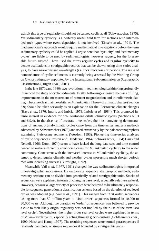
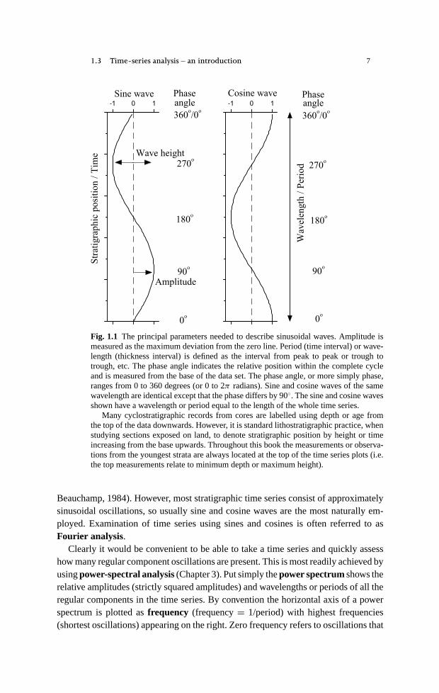
As shown in Fig. 1.1 a simple oscillation can be described in terms of itsamplitudeand wavelength. Additionally, the position within the oscillation or itsphase angleor phase(ranging from 0 to 360◦ or from 0 to 2π radians) can be measured fromsome sort of origin along the time or cumulative thickness/depth axis. Geologicallythe position of the origin is determined arbitrarily by wherever the data collectionstarted. However, mathematically this type of simple oscillation is usually describedusing a sinusoid; if it starts at the mid-point of an oscillation it is a sine wave andif it starts at a maximum it is a cosine wave (Fig. 1.1). Sine and cosine waves areconvenient for describing oscillations mathematically. To produce a sinusoid that startsat a phase angle of 45◦ it is only necessary to add together a sine and cosine wave ofthe same wavelength and the same amplitude (Fig. 1.2a). Any other starting angle canbe generated by controlling the relative amplitudes of the sine and cosine waves used(Fig. 1.2b). Observational time series rarely have oscillations of such a simple shape,but more complicated shapes, such as cuspate waves with narrow troughs and longpeaks, can be represented by adding sine and cosine waves with particular wavelengths(Section 5.2.4).

Observational time series are of course usually composed of many different wave-length oscillations. According toFourier’s theorem, any time series, no matter whatshape it is provided it has some oscillations and no infinite values, can be recreatedby adding together regular sine and cosine waves having the correct wavelengths andamplitudes. Sine and cosine waves form a set of so-calledorthogonal functions. Or-thogonal functions are simply groups of waves that can be added together to describeany time series, but none of the individual component waves can be constructed fromcombinations of other waves in the group. There are other sets of orthogonal functions,which can be used in place of sines and cosines (e.g.Walsh functions, Section 3.4.6,


Fig. 1.1 The principal parameters needed to describe sinusoidal waves. Amplitude ismeasured as the maximum deviation from the zero line. Period (time interval) or wave-length (thickness interval) is defined as the interval from peak to peak or trough totrough, etc. The phase angle indicates the relative position within the complete cycleand is measured from the base of the data set. The phase angle, or more simply phase,ranges from 0 to 360 degrees (or 0 to 2π radians). Sine and cosine waves of the samewavelength are identical except that the phase differs by 90◦. The sine and cosine wavesshown have a wavelength or period equal to the length of the whole time series.

Many cyclostratigraphic records from cores are labelled using depth or age fromthe top of the data downwards. However, it is standard lithostratigraphic practice, whenstudying sections exposed on land, to denote stratigraphic position by height or timeincreasing from the base upwards. Throughout this book the measurements or observa-tions from the youngest strata are always located at the top of the time series plots (i.e.the top measurements relate to minimum depth or maximum height).

Beauchamp, 1984). However, most stratigraphic time series consist of approximatelysinusoidal oscillations, so usually sine and cosine waves are the most naturally em-ployed. Examination of time series using sines and cosines is often referred to asFourier analysis.

Clearly it would be convenient to be able to take a time series and quickly assesshow many regular component oscillations are present. This is most readily achieved byusingpower-spectral analysis(Chapter 3). Put simply thepower spectrumshows therelative amplitudes (strictly squared amplitudes) and wavelengths or periods of all theregular components in the time series. By convention the horizontal axis of a powerspectrum is plotted asfrequency (frequency= 1/period) with highest frequencies(shortest oscillations) appearing on the right. Zero frequency refers to oscillations that

8 Introduction

Fig. 1.2 (a) When sine andcosine waves with the samewavelength and equalamplitude are addedtogether, the resultingsinusoid has a phase whichis intermediate between thatof the components (i.e. itdiffers by 45◦). (b) Adding asine wave with an amplitudeof one unit to a cosine wavewith an amplitude of half aunit produces a sinusoidwith a phase of 67.5◦. Thismeans that any sinusoid canbe considered to representthe sum of one sine and onecosine wave having thesame wavelength and thecorrect relative amplitudes.


have wavelengths or periods exceeding the length of the whole data set. If the data arecollected as a function of time, frequency is measured in ‘numbers of cycles per timeunit’ which is usually shortened to ‘cycles per time unit’ (e.g. cycles per thousandyears). If a thickness or depth scale is used then instead of frequency some authorsrefer to thewave number(i.e. wave number= 1/wavelength in thickness). However,for clarity in cyclostratigraphic studies it is usual for one to speak of frequency eventhough the units do not include a time element (e.g. cycles per metre).

Spectral analysis requires amplitude measurements determined as positive or neg-ative deviations from some zero line. However, although the zero line is sometimesdefined using the average or mean of the data, usually a more complicated defini-tion is involved as discussed later (Section 3.2). Consequently, it is often confusing,when inspecting a time series plot, if the zero line is indicated, so this has only beenillustrated for the time series in Figs. 1.1 and 1.2. Geologists often prefer to plotstratigraphic position or time running verticallyup the page. However, frequentlypalaeoceanographers and environmental scientists plot data relative to time so that thetime axis runs horizontally, with younger data on the left of the page. To simplifythe layout of the figures I have plotted all the time series the same way so that eitherstratigraphic position or time runs up the page, hence the youngest data are found atthe top.

The vertical axis of the spectrum is usually plotted as squared amplitude and byanalogy with physics it is described as ‘power’ (energy per time interval), hence thename power spectrum. Since amplitude refers to deviation from the zero line, squaredamplitude can be thought of as squared deviation and so sometimes one speaks ofthe variance spectrum (variance equals squared standard deviation). Occasionallyamplitude, rather than squared amplitude, is plotted against frequency, so creating anamplitude spectrum(also known as amagnitude spectrum). If small spectral peaksneed to be studied together with large peaks then the log of power is plotted againstfrequency. In electronic signal processing, for comparing power values thedecibelscaleis used (i.e. 10× log10power) so that a power value of 0.01 equals−20 dB. (Notethat for comparing voltages, analogous to amplitude in time-series analysis, decibelsare calculated as 20× log10voltage/amplitude.)

It is sometimes useful to be able to think of spectral analysis using physical analo-gies. Thus the rainbow effect produced by a glass prism acting on a beam of white lightis a classical example of a spectrum. The brightness of different parts of the rainbowcorresponds to the power and the various colours the frequency. The ear and brainsimilarly apparently analyse sound (fluctuating air pressure) as though it is a time se-ries made up of components with different amplitude/power (loudness) and frequency(pitch, Taylor, 1965, 1976). Thus different parts of the brain are activated by differentfrequencies, though the size of the response depends on musical training/skill and thetype of sound (e.g. Pantevet al., 1998).

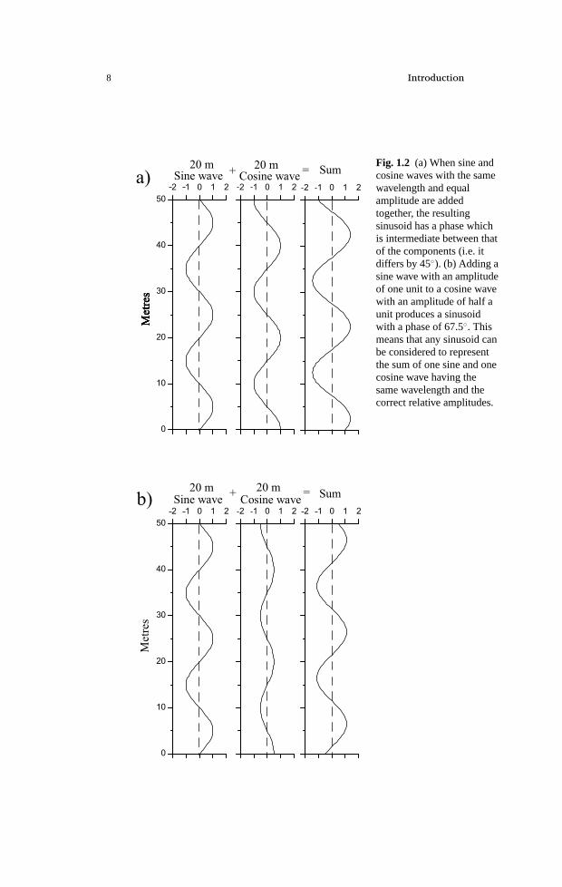
Figure 1.3 illustrates an example where a 10 m sine wave has been added to a 2.78 msine wave. The resulting time series, shown as ‘Sum’ on the right, would have lookeddifferent if the relative phase of the two components and/or the relative amplitudes

10 Introduction

Fig. 1.3 Adding sinusoidswith different wavelengthsproduces a time series withmultiple frequency com-ponents. Power spectra areused to: (a) identify whichfrequency components arepresent (frequency=1/wavelength); and(b) determine their relativeamplitudes. In this casetwo sine waves of equalamplitude, but differentwavelengths, have beenadded to produce the timeseries labelled “Sum”.The corresponding powerspectrum has peaks thatoccur at frequenciescorresponding to thecomponent wavelengths.The peaks are equal inheight because thecomponents have the sameamplitude. Note that it isimpossible to tell from thespectrum whether thecomponents are sine orcosine waves – in otherwords the spectrum isindependent of the phaseof the components.

differed. The power spectrum in Fig. 1.3 shows that the time series consists of just twofrequency components. When power spectra are generated all the phase informationis discarded. As a result, changing the relative positions or phases of the 2.78 m os-cillations relative to the 10.0 m oscillations, and hence the shape of the time series,would not influence the shape of the spectrum. The heights of the two spectral peaksin Fig. 1.3 are identical because the amplitudes of the component oscillations areidentical. The larger the spectral peak, the greater the amplitude of the correspondingwavelength of oscillation and the greater its ‘importance’ in controlling the overallshape of the time series. The frequency of the spectral peaks can be read from thehorizontal axis and indicates, of course, that oscillations with wavelengths of 10.00 mand 2.78 m are present in the time series.

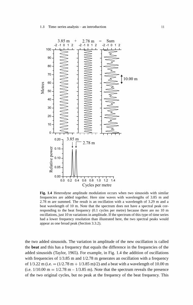
Sinusoids with varying amplitude are said to exhibitamplitude modulation orAM . There are two types of amplitude modulation. Inheterodyne AM the additionof two sinusoids with similar wavelengths creates a new single oscillation (Olsen,1977). The new oscillation has a frequency that is the average of the frequencies of


Fig. 1.4 Heterodyne amplitude modulation occurs when two sinusoids with similarfrequencies are added together. Here sine waves with wavelengths of 3.85 m and2.78 m are summed. The result is an oscillation with a wavelength of 3.29 m and abeat wavelength of 10 m. Note that the spectrum does not havea spectral peak cor-responding to the beat frequency (0.1 cycles per metre) because there are no 10 moscillations, just 10 m variations in amplitude. If the spectrum of this type of time serieshad a lower frequency resolution than illustrated here, the two spectral peaks wouldappear as one broad peak (Section 3.3.2).

the two added sinusoids. The variation in amplitude of the new oscillation is calledthebeat and this has a frequency that equals the difference in the frequencies of theadded sinusoids (Taylor, 1965). For example, in Fig. 1.4 the addition of oscillationswith frequencies of 1/3.85 m and 1/2.78 m generates an oscillation with a frequencyof 1/3.22 m (i.e.= (1/2.78 m+ 1/3.85 m)/2) and a beat with a wavelength of 10.00 m(i.e. 1/10.00 m= 1/2.78 m – 1/3.85 m). Note that the spectrum reveals the presenceof the two original cycles, but no peak at the frequency of the beat frequency. This

12 Introduction

is because there are no oscillations with a 10 m wavelength in the record, just 10 mvariations in amplitude.

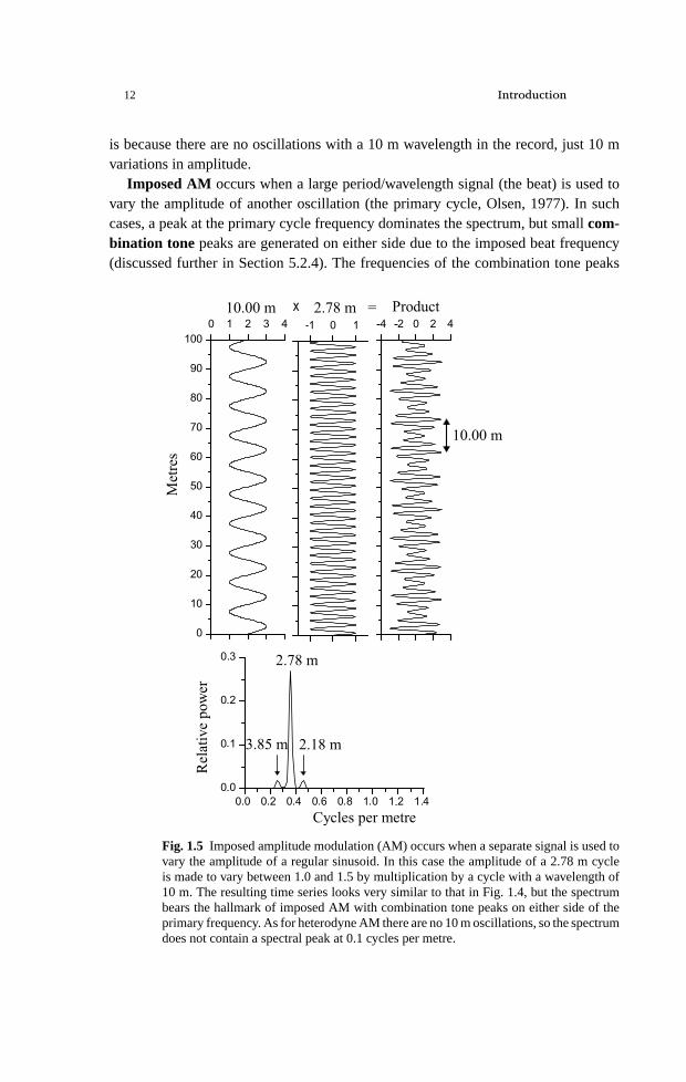
Imposed AM occurs when a large period/wavelength signal (the beat) is used tovary the amplitude of another oscillation (the primary cycle, Olsen, 1977). In suchcases, a peak at the primary cycle frequency dominates the spectrum, but smallcom-bination tone peaks are generated on either side due to the imposed beat frequency(discussed further in Section 5.2.4). The frequencies of the combination tone peaks

Fig. 1.5 Imposed amplitude modulation (AM)occurs when a separate signal is used tovary the amplitude of a regular sinusoid. In this case the amplitude of a 2.78 m cycleis made to vary between 1.0 and 1.5 by multiplication by a cycle with a wavelength of10 m. The resulting time series looks very similar to that in Fig. 1.4, but the spectrumbears the hallmark of imposed AM with combination tone peaks on either side of theprimary frequency. As for heterodyne AM there are no 10 m oscillations, so the spectrumdoes not contain a spectral peak at 0.1 cycles per metre.


Fig. 1.6 When three sinewavesof differentwavelengthsareadded together, the resultingtime series can look quite complicated. Nevertheless, as power spectra are unaffectedby phase, the three component wavelengths and their relative amplitudes are readilydetermined.

correspond to the primary oscillation frequency minus the beat frequency and to theprimary oscillation frequency plus the beat frequency (Taylor, 1965). In the exampleshown in Fig. 1.5, 10 m imposed AM of the 2.78 m oscillations generates sidebands atfrequencies of 1/3.85 m (i.e.= 1/2.78 m – 1/10.0 m) and 1/2.18 m (i.e.= 1/2.78 m+1/10.0m). As for heterodyneAM, the spectrumof an imposedAMsignal does not havea peak at the beat frequency because there are no 10 m oscillations present ( just 10 mvariations in amplitude). A crucial point is that power spectra reveal average power.Thus, except in rare clear-cut cases (e.g. Figs. 1.4 and 1.5), power spectra cannot beused to infer how the amplitude of an oscillation varies along the length of a time series.

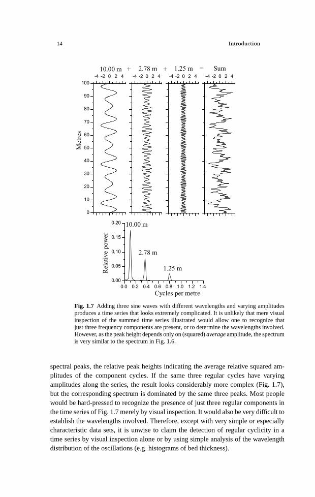
Time series can look exceedingly complicated when only a few regular cycles areadded together. In Fig. 1.6 the addition of three oscillations with different amplitudesresults in a moderately complicated looking data set. The spectrum contains three

14 Introduction

Fig. 1.7 Adding three sine waves with different wavelengths andvarying amplitudesproduces a time series that looks extremely complicated. It is unlikely that mere visualinspection of the summed time series illustrated would allow one to recognize thatjust three frequency components are present, or to determine the wavelengths involved.However, as the peak height depends only on (squared)averageamplitude, the spectrumis very similar to the spectrum in Fig. 1.6.

spectral peaks, the relative peak heights indicating the average relative squared am-plitudes of the component cycles. If the same three regular cycles have varyingamplitudes along the series, the result looks considerably more complex (Fig. 1.7),but the corresponding spectrum is dominated by the same three peaks. Most peoplewould be hard-pressed to recognize the presence of just three regular components inthe time series of Fig. 1.7 merely by visual inspection. It would also be very difficult toestablish the wavelengths involved. Therefore, except with very simple or especiallycharacteristic data sets, it is unwise to claim the detection of regular cyclicity in atime series by visual inspection alone or by using simple analysis of the wavelengthdistribution of the oscillations (e.g. histograms of bed thickness).


30oN

0o 30oE 60oE

Fig. 1.8 Location map for the cyclostratigraphic records illustrated in Chapters 1 to 5.Formn. denotes formation.

Observational time series usually consist of the addition of tens or hundreds ofregular sine and cosine components. This means that every possible regular frequencycomponent has a non-zero amplitude. Consequently, spectral analysis of stratigraphictime series is used to look for spectral peaks that emerge from a background of spectralvalues.

This is an appropriate point to introduce the data sets used to illustrate this book.They are listed, according to the age of the strata from which they were obtained,in Table 1.1. Figures 1.8 and 6.1 show where these cyclostratigraphic records wereobtained. Many of these records are based on oxygen-isotope records (see Faure,1986 for an introduction to the determination and uses ofδ18O and an explanationof the delta notation). One of the records has been selected to help illustrate the var-ious time series methods described in the book. The information comes from theEarly Jurassic hemipelagic formation called the Belemnite Marls, which is approxi-mately 190 million years old and exposed on the coast of Dorset, England (Fig. 1.8,Table 1.1, Weedon and Jenkyns, 1990, 1999). In the field much of this unit consistsof interbedded light-grey marls, dark-grey marls and brown-black laminated shales.These lithologies form decimetre-scale bedding couplets that are grouped into metre-scale bundles (Fig. 1.9). In several intervals at the base of the formation, the beddingis barely visible. Towards the top the couplets and bundles are noticeably thinner(Fig. 1.9).

As forall stratigraphic recordsobtained from theJurassic system, theabsolutedatinguncertainties create difficulties when assessing the duration of processes lasting less

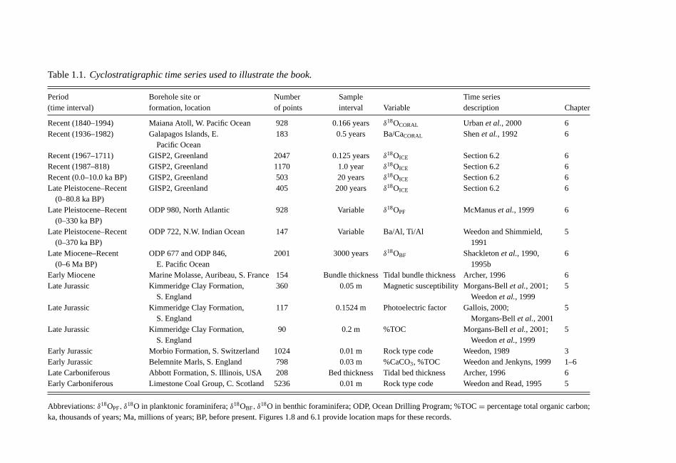
Table 1.1.Cyclostratigraphic time series used to illustrate the book.

Period Borehole site or Number Sample Time series(time interval) formation, location of points interval Variable description Chapter

Recent (1840–1994) Maiana Atoll, W. Pacific Ocean 928 0.166 yearsδ18OCORAL Urbanet al., 2000 6Recent (1936–1982) Galapagos Islands, E.

Pacific Ocean183 0.5 years Ba/CaCORAL Shenet al., 1992 6

Recent (1967–1711) GISP2, Greenland 2047 0.125 yearsδ18OICE Section 6.2 6Recent (1987–818) GISP2, Greenland 1170 1.0 year δ18OICE Section 6.2 6Recent (0.0–10.0 ka BP) GISP2, Greenland 503 20 yearsδ18OICE Section 6.2 6Late Pleistocene–Recent

(0–80.8 ka BP)GISP2, Greenland 405 200 years δ18OICE Section 6.2 6

Late Pleistocene–Recent(0–330 ka BP)

ODP 980, North Atlantic 928 Variable δ18OPF McManuset al., 1999 6

Late Pleistocene–Recent(0–370 ka BP)

ODP 722, N.W. Indian Ocean 147 Variable Ba/Al, Ti/Al Weedon and Shimmield,1991

5

Late Miocene–Recent(0–6 Ma BP)

ODP 677 and ODP 846,E. Pacific Ocean

2001 3000 years δ18OBF Shackletonet al., 1990,1995b

6

Early Miocene Marine Molasse, Auribeau, S. France 154 Bundle thickness Tidal bundle thickness Archer, 1996 6Late Jurassic Kimmeridge Clay Formation,

S. England360 0.05 m Magnetic susceptibility Morgans-Bellet al., 2001;

Weedonet al., 19995

Late Jurassic Kimmeridge Clay Formation,S. England

117 0.1524 m Photoelectric factor Gallois, 2000;Morgans-Bellet al., 2001

5

Late Jurassic Kimmeridge Clay Formation,S. England

90 0.2 m %TOC Morgans-Bellet al., 2001;Weedonet al., 1999

5

Early Jurassic Morbio Formation, S. Switzerland 1024 0.01 m Rock type code Weedon, 1989 3Early Jurassic Belemnite Marls, S. England 798 0.03 m %CaCO3, %TOC Weedon and Jenkyns, 1999 1–6Late Carboniferous Abbott Formation, S. Illinois, USA 208 Bed thickness Tidal bed thickness Archer, 1996 6Early Carboniferous Limestone Coal Group, C. Scotland 5236 0.01 m Rock type code Weedon and Read, 1995 5

Abbreviations:δ18OPF, δ18O in planktonic foraminifera;δ18OBF, δ

18O in benthic foraminifera; ODP, Ocean Drilling Program; %TOC= percentage total organic carbon;ka, thousands of years; Ma, millions of years; BP, before present. Figures 1.8 and 6.1 provide location maps for these records.


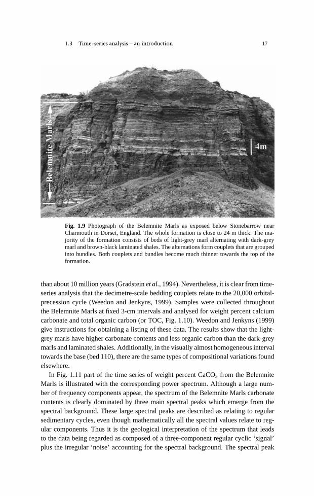
Fig. 1.9 Photograph of the Belemnite Marls as exposed below Stonebarrow nearCharmouth in Dorset, England. The whole formation is close to 24 m thick. The ma-jority of the formation consists of beds of light-grey marl alternating with dark-greymarl and brown-black laminated shales. The alternations form couplets that are groupedinto bundles. Both couplets and bundles become much thinner towards the top of theformation.

than about 10 million years (Gradsteinet al., 1994). Nevertheless, it is clear from time-series analysis that the decimetre-scale bedding couplets relate to the 20,000 orbital-precession cycle (Weedon and Jenkyns, 1999). Samples were collected throughoutthe Belemnite Marls at fixed 3-cm intervals and analysed for weight percent calciumcarbonate and total organic carbon (or TOC, Fig. 1.10). Weedon and Jenkyns (1999)give instructions for obtaining a listing of these data. The results show that the light-grey marls have higher carbonate contents and less organic carbon than the dark-greymarls and laminated shales. Additionally, in the visually almost homogeneous intervaltowards the base (bed 110), there are the same types of compositional variations foundelsewhere.

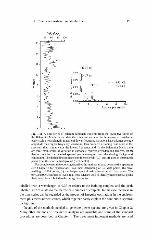
In Fig. 1.11 part of the time series of weight percent CaCO3 from the BelemniteMarls is illustrated with the corresponding power spectrum. Although a large num-ber of frequency components appear, the spectrum of the Belemnite Marls carbonatecontents is clearly dominated by three main spectral peaks which emerge from thespectral background. These large spectral peaks are described as relating to regularsedimentary cycles, even though mathematically all the spectral values relate to reg-ular components. Thus it is the geological interpretation of the spectrum that leadsto the data being regarded as composed of a three-component regular cyclic ‘signal’plus the irregular ‘noise’ accounting for the spectral background. The spectral peak

18 Introduction

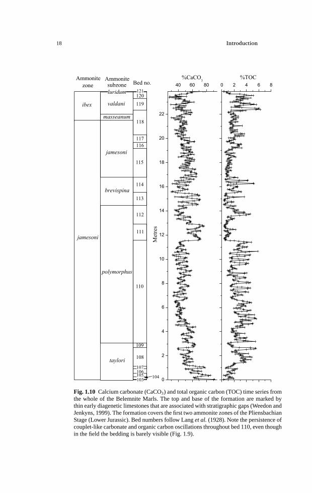
Fig. 1.10 Calcium carbonate (CaCO3) and total organic carbon (TOC) time series fromthe whole of the Belemnite Marls. The top and base of the formation are marked bythin early diagenetic limestones that are associated with stratigraphic gaps (Weedon andJenkyns, 1999). The formation covers the first two ammonite zones of the PliensbachianStage (Lower Jurassic). Bed numbers follow Langet al.(1928). Note the persistence ofcouplet-like carbonate and organic carbon oscillations throughout bed 110, even thoughin the field the bedding is barely visible (Fig. 1.9).


Fig. 1.11 A time series of calcium carbonate contents from the lower two-thirds ofthe Belemnite Marls. In real data there is some variation in the measured variable atevery scale or wavelength. In general, lower frequency variations have a larger averageamplitude than higher frequency variations. This produces a sloping continuum in thespectrum that rises towards the lowest frequency end. In the Belemnite Marls thereare three main scales of variation in carbonate contents (Weedon and Jenkyns, 1999)that account for the labelled spectral peaks emerging from the sloping backgroundcontinuum. The dashed lines indicate confidence levels (CL) and are used to distinguishpeaks from the spectral background (Section 3.5).

For completeness the following describes the methods used to generate this spectrum(see Chapter 3 for explanations): (a) linear detrending of 548 data points, (b) zero-padding to 1024 points, (c) multi-taper spectral estimation using six data tapers. The95% and 99% confidence levels (e.g. 99% CL) are used to identify those spectral peaksthat cannot be attributed to the background noise.

labelled with a wavelength of 0.37 m relates to the bedding couplets and the peaklabelled 3.07 m relates to the metre-scale bundles of couplets. In this case the noise inthe time series can be regarded as the product of irregular oscillations in the environ-ment plus measurement errors, which together partly explain the continuous spectralbackground.

Details of the methods needed to generate power spectra are given in Chapter 3.Many other methods of time-series analysis are available and some of the standardprocedures are described in Chapter 4. The three most important methods are used

20 Introduction

to: (a) isolate regular cycles from the time series (filtering); (b) examine variationsin cycle amplitude (amplitude demodulation); and (c) study the phase and amplituderelationships of pairs of variables obtained simultaneously from the same samples ortime intervals (i.e. cross-spectral analysis). Chapter 5 is concerned with distortions ofthese environmental signals as recorded stratigraphically, as well as practical consid-erations in conducting time-series analyses of real data. Chapter 6 discusses the manyenvironmental origins for the regular cycles that have been observed in stratigraphicrecords (from tidal to Milankovitch cycles).

In the context of cyclostratigraphic data sets, spectral analysis is usually the firstprocedure used, because it allows the detection of regular cyclicity and determinationof wavelengths and average amplitudes. However, before the difficulties of generatingand interpreting power spectra can be considered, it is essential that one is aware ofthe many issues concerning the construction of time series (Chapter 2).

1.4 Chapter overview

� Time-series analysis provides procedures for examining quantitative records ofenvironmental variability. It was widely adopted in cyclostratigraphic studiesfollowing the vindication of the orbital-climatic theory (Milankovitch theory) inthe early 1980s.

� Spectral analysis allows the detection of multiple regular cycles in a time series.Each regular component is characterized in terms of its frequency (= 1/periodor 1/wavelength) andaveragepower (= squared average amplitude).

� Regular amplitude modulation in a time series doesnotgenerate a spectral peakat the modulation frequency.

Time-SeriesAnalysis andCyclostratigraphycatdir.loc.gov/catdir/samples/cam033/2002067374.pdf ·...

Documents

Transcript of Time-SeriesAnalysis andCyclostratigraphycatdir.loc.gov/catdir/samples/cam033/2002067374.pdf ·...