Time Series Forecasting Using Novel Feature Extraction Algorithm and Multilayer Neural Network

International Journal of Computer Applications Technology and Research

Volume 5 –Issue 12, 748-759, 2016, ISSN:-2319–8656

www.ijcat.com 748

Time Series Forecasting Using Novel Feature Extraction Algorithm and Multilayer Neural Network

Raheleh Rezazadeh

Master student of software Engineering, Ferdows

Islamic Islamic Azad University,

Ferdows, Iran

Hooman Kashanian

Department of Computer science and software

Engineering

Islamic Azad University,

Ferdows, Iran

Abstract: Time series forecasting is important because it can often provide the foundation for decision making in a large variety of

fields. A tree-ensemble method, referred to as time series forest (TSF), is proposed for time series classification. The approach is based

on the concept of data series envelopes and essential attributes generated by a multilayer neural network... These claims are further

investigated by applying statistical tests. With the results presented in this article and results from related investigations that are

considered as well, we want to support practitioners or scholars in answering the following question: Which measure should be looked

at first if accuracy is the most important criterion, if an application is time-critical, or if a compromise is needed? In this paper

demonstrated feature extraction by novel method can improvement in time series data forecasting process.

Keyword: time series data, neural network, forecasting

www.ijcat.com 749

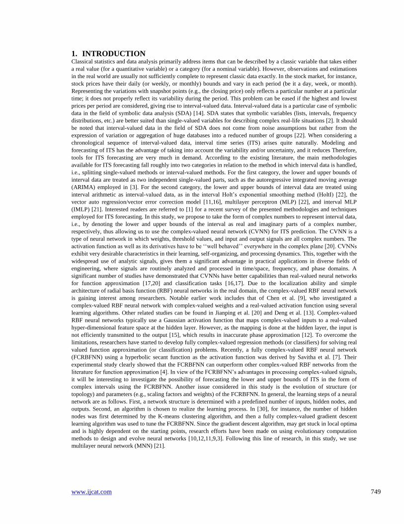
1. INTRODUCTION Classical statistics and data analysis primarily address items that can be described by a classic variable that takes either

a real value (for a quantitative variable) or a category (for a nominal variable). However, observations and estimations

in the real world are usually not sufficiently complete to represent classic data exactly. In the stock market, for instance,

stock prices have their daily (or weekly, or monthly) bounds and vary in each period (be it a day, week, or month).

Representing the variations with snapshot points (e.g., the closing price) only reflects a particular number at a particular

time; it does not properly reflect its variability during the period. This problem can be eased if the highest and lowest

prices per period are considered, giving rise to interval-valued data. Interval-valued data is a particular case of symbolic

data in the field of symbolic data analysis (SDA) [14]. SDA states that symbolic variables (lists, intervals, frequency

distributions, etc.) are better suited than single-valued variables for describing complex real-life situations [2]. It should

be noted that interval-valued data in the field of SDA does not come from noise assumptions but rather from the

expression of variation or aggregation of huge databases into a reduced number of groups [22]. When considering a

chronological sequence of interval-valued data, interval time series (ITS) arises quite naturally. Modeling and

forecasting of ITS has the advantage of taking into account the variability and/or uncertainty, and it reduces Therefore,

tools for ITS forecasting are very much in demand. According to the existing literature, the main methodologies

available for ITS forecasting fall roughly into two categories in relation to the method in which interval data is handled,

i.e., splitting single-valued methods or interval-valued methods. For the first category, the lower and upper bounds of

interval data are treated as two independent single-valued parts, such as the autoregressive integrated moving average

(ARIMA) employed in [3]. For the second category, the lower and upper bounds of interval data are treated using

interval arithmetic as interval-valued data, as in the interval Holt‟s exponential smoothing method (HoltI) [22], the

vector auto regression/vector error correction model [11,16], multilayer perceptron (MLP) [22], and interval MLP

(IMLP) [21]. Interested readers are referred to [1] for a recent survey of the presented methodologies and techniques

employed for ITS forecasting. In this study, we propose to take the form of complex numbers to represent interval data,

i.e., by denoting the lower and upper bounds of the interval as real and imaginary parts of a complex number,

respectively, thus allowing us to use the complex-valued neural network (CVNN) for ITS prediction. The CVNN is a

type of neural network in which weights, threshold values, and input and output signals are all complex numbers. The

activation function as well as its derivatives have to be „„well behaved‟‟ everywhere in the complex plane [20]. CVNNs

exhibit very desirable characteristics in their learning, self-organizing, and processing dynamics. This, together with the

widespread use of analytic signals, gives them a significant advantage in practical applications in diverse fields of

engineering, where signals are routinely analyzed and processed in time/space, frequency, and phase domains. A

significant number of studies have demonstrated that CVNNs have better capabilities than real-valued neural networks

for function approximation [17,20] and classification tasks [16,17]. Due to the localization ability and simple

architecture of radial basis function (RBF) neural networks in the real domain, the complex-valued RBF neural network

is gaining interest among researchers. Notable earlier work includes that of Chen et al. [9], who investigated a

complex-valued RBF neural network with complex-valued weights and a real-valued activation function using several

learning algorithms. Other related studies can be found in Jianping et al. [20] and Deng et al. [13]. Complex-valued

RBF neural networks typically use a Gaussian activation function that maps complex-valued inputs to a real-valued

hyper-dimensional feature space at the hidden layer. However, as the mapping is done at the hidden layer, the input is

not efficiently transmitted to the output [15], which results in inaccurate phase approximation [12]. To overcome the

limitations, researchers have started to develop fully complex-valued regression methods (or classifiers) for solving real

valued function approximation (or classification) problems. Recently, a fully complex-valued RBF neural network

(FCRBFNN) using a hyperbolic secant function as the activation function was derived by Savitha et al. [7]. Their

experimental study clearly showed that the FCRBFNN can outperform other complex-valued RBF networks from the

literature for function approximation [4]. In view of the FCRBFNN‟s advantages in processing complex-valued signals,

it will be interesting to investigate the possibility of forecasting the lower and upper bounds of ITS in the form of

complex intervals using the FCRBFNN. Another issue considered in this study is the evolution of structure (or

topology) and parameters (e.g., scaling factors and weights) of the FCRBFNN. In general, the learning steps of a neural

network are as follows. First, a network structure is determined with a predefined number of inputs, hidden nodes, and

outputs. Second, an algorithm is chosen to realize the learning process. In [30], for instance, the number of hidden

nodes was first determined by the K-means clustering algorithm, and then a fully complex-valued gradient descent

learning algorithm was used to tune the FCRBFNN. Since the gradient descent algorithm, may get stuck in local optima

and is highly dependent on the starting points, research efforts have been made on using evolutionary computation

methods to design and evolve neural networks [10,12,11,9,3]. Following this line of research, in this study, we use

multilayer neural network (MNN) [21].

www.ijcat.com 750

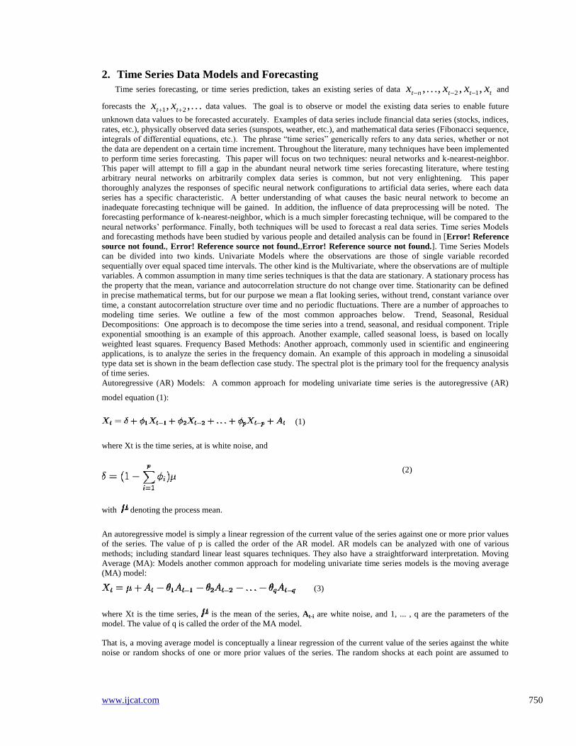
2. Time Series Data Models and Forecasting

Time series forecasting, or time series prediction, takes an existing series of data tttnt xxxx ,,,, 12 and

forecasts the ,, 21 tt xx data values. The goal is to observe or model the existing data series to enable future

unknown data values to be forecasted accurately. Examples of data series include financial data series (stocks, indices,

rates, etc.), physically observed data series (sunspots, weather, etc.), and mathematical data series (Fibonacci sequence,

integrals of differential equations, etc.). The phrase “time series” generically refers to any data series, whether or not

the data are dependent on a certain time increment. Throughout the literature, many techniques have been implemented

to perform time series forecasting. This paper will focus on two techniques: neural networks and k-nearest-neighbor.

This paper will attempt to fill a gap in the abundant neural network time series forecasting literature, where testing

arbitrary neural networks on arbitrarily complex data series is common, but not very enlightening. This paper

thoroughly analyzes the responses of specific neural network configurations to artificial data series, where each data

series has a specific characteristic. A better understanding of what causes the basic neural network to become an

inadequate forecasting technique will be gained. In addition, the influence of data preprocessing will be noted. The

forecasting performance of k-nearest-neighbor, which is a much simpler forecasting technique, will be compared to the

neural networks‟ performance. Finally, both techniques will be used to forecast a real data series. Time series Models

and forecasting methods have been studied by various people and detailed analysis can be found in [Error! Reference

source not found., Error! Reference source not found.,Error! Reference source not found.]. Time Series Models

can be divided into two kinds. Univariate Models where the observations are those of single variable recorded

sequentially over equal spaced time intervals. The other kind is the Multivariate, where the observations are of multiple

variables. A common assumption in many time series techniques is that the data are stationary. A stationary process has

the property that the mean, variance and autocorrelation structure do not change over time. Stationarity can be defined

in precise mathematical terms, but for our purpose we mean a flat looking series, without trend, constant variance over

time, a constant autocorrelation structure over time and no periodic fluctuations. There are a number of approaches to

modeling time series. We outline a few of the most common approaches below. Trend, Seasonal, Residual

Decompositions: One approach is to decompose the time series into a trend, seasonal, and residual component. Triple

exponential smoothing is an example of this approach. Another example, called seasonal loess, is based on locally

weighted least squares. Frequency Based Methods: Another approach, commonly used in scientific and engineering

applications, is to analyze the series in the frequency domain. An example of this approach in modeling a sinusoidal

type data set is shown in the beam deflection case study. The spectral plot is the primary tool for the frequency analysis

of time series.

Autoregressive (AR) Models: A common approach for modeling univariate time series is the autoregressive (AR)

model equation (1):

(1)

where Xt is the time series, at is white noise, and

(2)

with denoting the process mean.

An autoregressive model is simply a linear regression of the current value of the series against one or more prior values

of the series. The value of p is called the order of the AR model. AR models can be analyzed with one of various

methods; including standard linear least squares techniques. They also have a straightforward interpretation. Moving

Average (MA): Models another common approach for modeling univariate time series models is the moving average

(MA) model:

(3)

where Xt is the time series, is the mean of the series, At-i are white noise, and 1, ... , q are the parameters of the

model. The value of q is called the order of the MA model.

That is, a moving average model is conceptually a linear regression of the current value of the series against the white

noise or random shocks of one or more prior values of the series. The random shocks at each point are assumed to

www.ijcat.com 751

come from the same distribution, typically a normal distribution, with location at zero and constant scale. The

distinction in this model is that these random shocks are propagated to future values of the time series. Fitting the MA

estimates is more complicated than with AR models because the error terms are not observable. This means that

iterative non-linear fitting procedures need to be used in place of linear least squares. MA models also have a less

obvious interpretation than AR models. Note, however, that the error terms after the model is fit should be independent

and follow the standard assumptions for a univariate process.

Box-Jenkins Approach: The Box-Jenkins ARMA model is a combination of the AR and MA models:

(4)

where the terms in the equation have the same meaning as given for the AR and MA model [Error! Reference source

not found.].

The Box-Jenkins model assumes that the time series is stationary. Box and Jenkins recommend differencing non-

stationary series one or more times to achieve stationarity. Doing so produces an ARIMA model, with the "I" standing

for "Integrated". Some formulations transform the series by subtracting the mean of the series from each data point.

This yields a series with a mean of zero. Whether you need to do this or not is dependent on the software you use to

estimate the model. Box-Jenkins models can be extended to include seasonal autoregressive and seasonal moving

average terms. Although this complicates the notation and mathematics of the model, the underlying concepts for

seasonal autoregressive and seasonal moving average terms are similar to the non-seasonal autoregressive and moving

average terms. The most general Box-Jenkins model includes difference operators, autoregressive terms, moving

average terms, seasonal difference operators, seasonal autoregressive terms, and seasonal moving average terms. As

with modeling in general, however, only necessary terms should be included in the model.

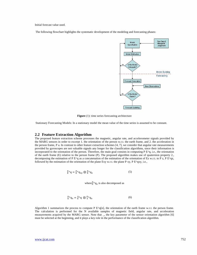
2.1 Steps in the Time Series Forecasting Process: The goal of a time series forecast is to identify factors that can be predicted. This is a systematic approach involving the

following steps and show in Figure (1).

Step 1: Hypothesize a form for the time series model.

Identify which of the time series components should be included in the model.

Perform the following operations.

Collect historical data.

Graph the data vs. time.

Hypothesize a form for the time series model.

Verify this hypothesis statistically.

Step 2: Select a forecasting technique. A forecasting technique must be chosen to predict future values of the time

series.

The values of input parameters must be determined before the technique can be applied.

Step 3: Prepare a forecast.

The appropriate data values must be substituted into the selected forecasting model.

The forecast may be affected by Number of past observations used.

www.ijcat.com 752

Initial forecast value used.

The following flowchart highlights the systematic development of the modeling and forecasting phases:

Figure (1): time series forecasting architecture

Stationary Forecasting Models: In a stationary model the mean value of the time series is assumed to be constant.

2.2 Feature Extraction Algorithm The proposed feature extraction scheme processes the magnetic, angular rate, and accelerometer signals provided by

the MARG sensors in order to excerpt 1. the orientation of the person w.r.t. the earth frame, and 2. the acceleration in

the person frame, P a. In contrast to other feature extraction schemes [4, 7], we consider that angular rate measurements

provided by gyroscopes are not valuable signals any longer for the classification algorithms, since their information is

incorporated to the orientation of the person. Therefore, the main goal consists in computing P E^q, i.e., the orientation

of the earth frame (E) relative to the person frame (P). The proposed algorithm makes use of quaternion property 2.,

decomposing the estimation of P E^q as a concatenation of the estimation of the orientation of Ez w.r.t. to P z, P E^qz,

followed by the estimation of the orientation of the plane Exy w.r.t. the plane P xy, P E^qxy, i.e.,

(5)

where is also decomposed as

(6)

Algorithm 1 summarizes the process to compute P E^q[n], the orientation of the earth frame w.r.t. the person frame.

The calculation is performed for the N available samples of magnetic field, angular rate, and acceleration

measurements acquired by the MARG sensor. Note that _, the key parameter of the sensor orientation algorithm [6]

must be selected at the beginning, and it plays a key role in the performance of the classification algorithm.

www.ijcat.com 753

Algorithm 1 Pseudocode of person orientation algorithm

Select β

for n = 1: N do

Compute with the algorithm of [6] and β

Detect whether the person is walking

if walking then

Update

Update

else

end if

end for

2.3

2.4

2.5

Table 1Beginning parameters for heuristically trained neural networks.

Heuristic Algorithm Training

Update Frequency = 50, Change Frequency = 10, Decrement = 0.05

Architecture Learning

Rate

Epochs

Limit

Error

Limit

Data Series

O = original

L = less noisy

M = more noisy

A = ascending

Training Set

Data Point

Range (# of

Examples)

Validation Set

Data Point Range

(# of Examples)

35:20:1 0.3 500,000 1x10-10 O, L, M, A 0 – 143 (109) 144 – 215 (37)

35:10:1 0.3 500,000 1x10-10 O, L, M, A 0 – 143 (109) 144 – 215 (37)

35:2:1 0.3 500,000 1x10-10 O, L, M, A 0 – 143 (109) 144 – 215 (37)

25:20:1 0.3 250,000 1x10-10 O 0 – 143 (119) 144 – 215 (47)

25:10:1 0.3 250,000 1x10-10 O 0 – 143 (119) 144 – 215 (47)

www.ijcat.com 754

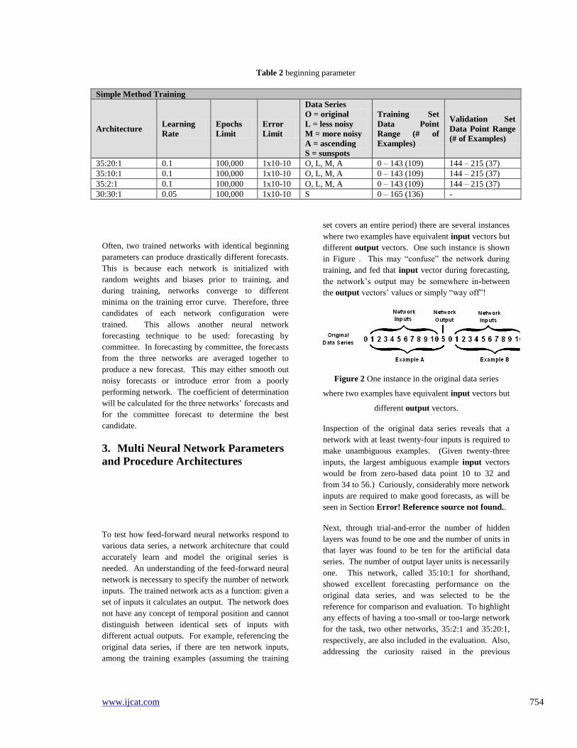
Table 2 beginning parameter

Simple Method Training


Rate

Epochs

Limit

Error

Limit

Data Series

O = original

L = less noisy

M = more noisy

A = ascending

S = sunspots

Training Set

Data Point

Range (# of

Examples)

Validation Set

Data Point Range

(# of Examples)

35:20:1 0.1 100,000 1x10-10 O, L, M, A 0 – 143 (109) 144 – 215 (37)

35:10:1 0.1 100,000 1x10-10 O, L, M, A 0 – 143 (109) 144 – 215 (37)

35:2:1 0.1 100,000 1x10-10 O, L, M, A 0 – 143 (109) 144 – 215 (37)

30:30:1 0.05 100,000 1x10-10 S 0 – 165 (136) -

Often, two trained networks with identical beginning

parameters can produce drastically different forecasts.

This is because each network is initialized with

random weights and biases prior to training, and

during training, networks converge to different

minima on the training error curve. Therefore, three

candidates of each network configuration were

trained. This allows another neural network

forecasting technique to be used: forecasting by

committee. In forecasting by committee, the forecasts

from the three networks are averaged together to

produce a new forecast. This may either smooth out

noisy forecasts or introduce error from a poorly

performing network. The coefficient of determination

will be calculated for the three networks‟ forecasts and

for the committee forecast to determine the best

candidate.

3. Multi Neural Network Parameters

and Procedure Architectures

To test how feed-forward neural networks respond to

various data series, a network architecture that could

accurately learn and model the original series is

needed. An understanding of the feed-forward neural

network is necessary to specify the number of network

inputs. The trained network acts as a function: given a

set of inputs it calculates an output. The network does

not have any concept of temporal position and cannot

distinguish between identical sets of inputs with

different actual outputs. For example, referencing the

original data series, if there are ten network inputs,

among the training examples (assuming the training

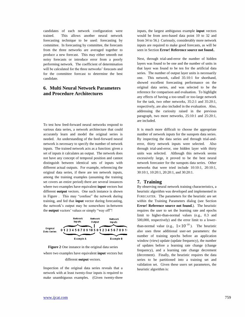
set covers an entire period) there are several instances

where two examples have equivalent input vectors but

different output vectors. One such instance is shown

in Figure . This may “confuse” the network during

training, and fed that input vector during forecasting,

the network‟s output may be somewhere in-between

the output vectors‟ values or simply “way off”!

Figure 2 One instance in the original data series


different output vectors.

Inspection of the original data series reveals that a

network with at least twenty-four inputs is required to

make unambiguous examples. (Given twenty-three

inputs, the largest ambiguous example input vectors

would be from zero-based data point 10 to 32 and

from 34 to 56.) Curiously, considerably more network

inputs are required to make good forecasts, as will be

seen in Section Error! Reference source not found..

Next, through trial-and-error the number of hidden

layers was found to be one and the number of units in

that layer was found to be ten for the artificial data

series. The number of output layer units is necessarily

one. This network, called 35:10:1 for shorthand,

showed excellent forecasting performance on the

original data series, and was selected to be the

reference for comparison and evaluation. To highlight

any effects of having a too-small or too-large network

for the task, two other networks, 35:2:1 and 35:20:1,

respectively, are also included in the evaluation. Also,

addressing the curiosity raised in the previous

www.ijcat.com 755

paragraph, two more networks, 25:10:1 and 25:20:1,

are included.

It is much more difficult to choose the appropriate

number of network inputs for the sunspots data series.

By inspecting the data series and through trial-and-

error, thirty network inputs were selected. Also

through trial-and-error, one hidden layer with thirty

units was selected. Although this network seems

excessively large, it proved to be the best neural

network forecaster for the sunspots data series. Other

networks that were tried include 10:10:1, 20:10:1,

30:10:1, 10:20:1, 20:20:1, and 30:20:1.

4. Training By observing neural network training characteristics, a

heuristic algorithm was developed and implemented in

FORECASTER. The parameters for the heuristic are set

within the Training Parameters dialog (see Section

Error! Reference source not found.). The heuristic

requires the user to set the learning rate and epochs

limit to higher-than-normal values (e.g., 0.3 and

500,000, respectively) and the error limit to a lower-

than-normal value (e.g., 10101 ). The heuristic

also uses three additional user-set parameters: the

number of training epochs before an application

window (view) update (update frequency), the number

of updates before a learning rate change (change

frequency), and a learning rate change decrement

(decrement). Finally, the heuristic requires the data

series to be partitioned into a training set and

validation set. Given these users set parameters, the

heuristic algorithm is:

for each view-update during training

if the validation error is higher than the lowest

value seen

increment count

if count equals change-frequency

if the learning rate minus decrement is

greater than zero

lower the learning rate by

decrement

reset count

continue

else

stop training

The purpose of the heuristic is to start with an

aggressive learning rate, which will quickly find a

coarse solution, and then to gradually decrease the

learning rate to find a finer solution. Of course, this

could be done manually by observing the validation

error and using the Change Training Parameters dialog

to alter the learning rate. But an automated solution is

preferred, especially for an empirical evaluation.

In the evaluation, the heuristic algorithm is compared

to the “simple” method of training where training

continues until either the number of epochs grows to

the epochs limit or the total squared error drops to the

error limit. Networks trained with the heuristic

algorithm are termed “heuristically trained”; networks

trained with the simple method are termed “simply

trained”.

Finally, the data series in Section Error! Reference

source not found. are partitioned so that the training

set is the first two periods and the validation set is the

third period. Note that “period” is used loosely for

less noisy, noisier, and ascending, since they are not

strictly periodic.

5. Simply Trained Neural Networks

with Thirty-Five Inputs Figure graphically shows the one-period forecasting

accuracy for the best candidates for simply trained

35:2:1, 35:10:1, and 35:20:1 networks. Figure (a),

(b), and (c) show forecasts from networks trained on

www.ijcat.com 756

the original, less noisy, and more noisy data series,

respectively, and the forecasts are compared to a

period of the original data series. Figure (d) shows

forecasts from networks trained on the ascending data

series, and the forecasts are compared to a fourth

“period” of the ascending series. In Figure (c) the

35:2:1 network is not included.

Figure graphically compares metrics for the best

candidates for simply trained 35:2:1, 35:10:1, and

35:20:1 networks. Figure (a) and (b) compare the

total squared error and unscaled error, respectively,

and (c) compares the coefficient of determination.

The vertical axis in (a) and (b) is logarithmic. The

number of epochs and training time are not included in

Figure because all networks were trained to 100,000

epochs.

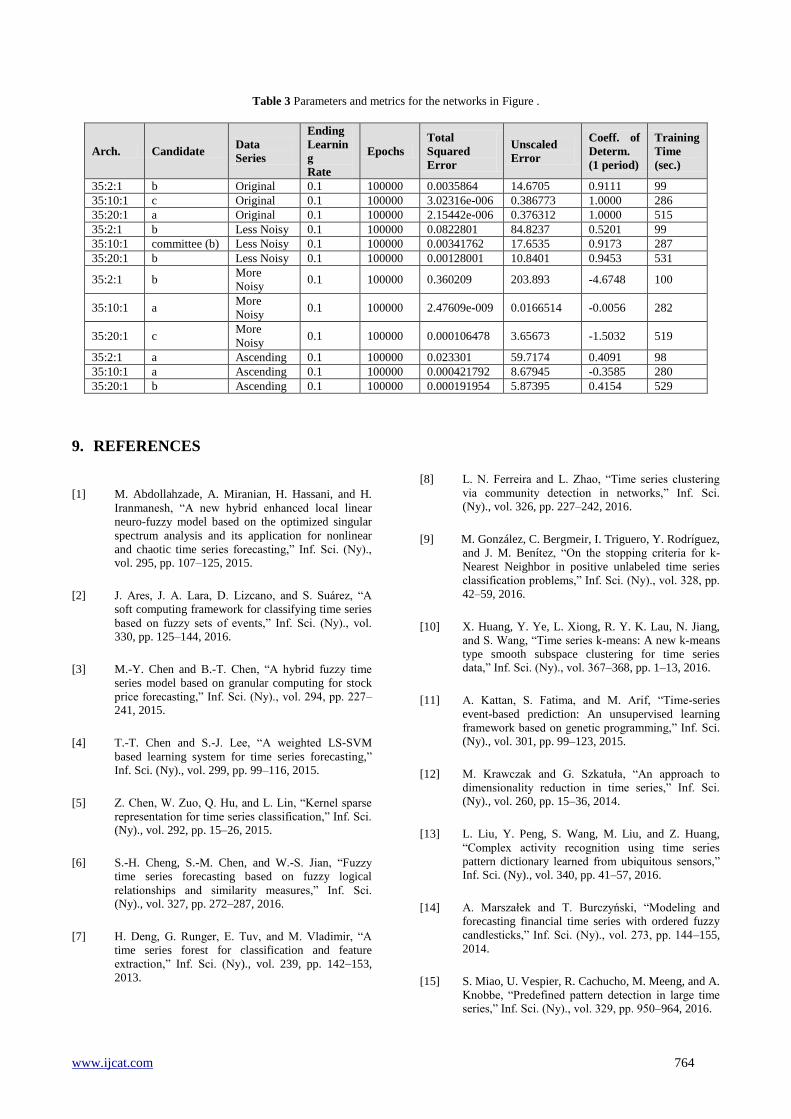
Finally, Table lists the raw data for the charts in

Figure and other parameters used in training. Refer to

Error! Reference source not found. for more

parameters.

In this case, it seems the heuristic was inappropriate.

Notice that the heuristic allowed the 35:2:1 network to

train for 28,850 epochs more than the simple method.

Also, the total squared error and unscaled error for the

heuristically trained network were lower, but so was

the coefficient of determination it was much lower.

Again, the forecasts for the 35:10:1 and 35:20:1

networks are near perfect, and are indistinguishable

from the original data series.

In Figure (b) the 35:2:1 network forecast is worse

than in Error! Reference source not found. (b),

whereas the 35:10:1 and 35:20:1 forecasts are about

the same as before. Notice that the 35:10:1 forecast is

from the committee, but does not appear to smooth the

data series‟ sharp transitions.

In Figure (c), the 35:2:1 network is not included

because of its poor forecasting performance on the

more noisy data series. The 35:10:1 and 35:20:1

forecasts are slightly worse than before.

In Figure (d), the 35:2:1 network is included and its

coefficient of determination is much improved from

before. The 35:10:1 and 35:20:1 network forecasts are

decent, despite the low coefficient of determination for

35:10:1. The forecasts appear to be shifted up when

compared to those in Error! Reference source not

found. (d).

Finally, by evaluating the charts in Figure and data in

Table some observations can be made:

The total squared error and unscaled error are higher

for noisy data series with the exception of the 35:10:1

network trained on the noisier data series. It trained to

extremely low errors, orders of magnitude lower than

with the heuristic, but its coefficient of determination

is also lower. This is probably an indication of

overfitting the noisier data series with simple training,

which hurt its forecasting performance.

The errors do not appear to correlate well with the

coefficient of determination.

In most cases, the committee forecast is worse than the

best candidate‟s forecast.

There are four networks whose coefficient of

determination is negative, compared with two for the

heuristic training method.

www.ijcat.com 757

(a)

(b)

(c)

(d)

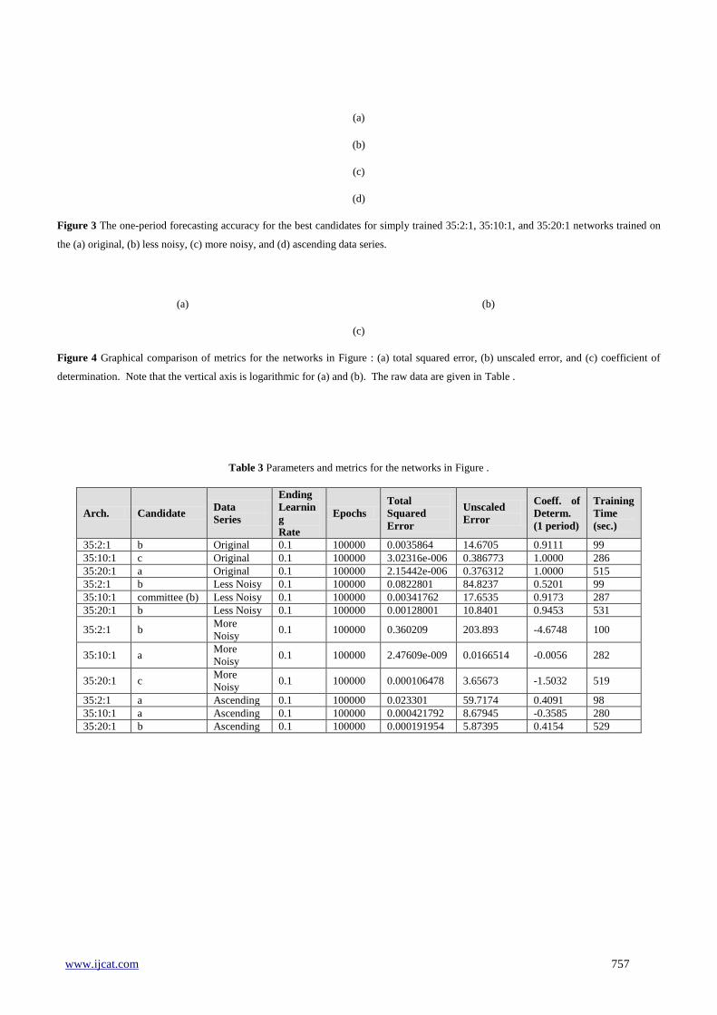
Figure 3 The one-period forecasting accuracy for the best candidates for simply trained 35:2:1, 35:10:1, and 35:20:1 networks trained on

the (a) original, (b) less noisy, (c) more noisy, and (d) ascending data series.

(a) (b)

(c)

Figure 4 Graphical comparison of metrics for the networks in Figure : (a) total squared error, (b) unscaled error, and (c) coefficient of

determination. Note that the vertical axis is logarithmic for (a) and (b). The raw data are given in Table .

Table 3 Parameters and metrics for the networks in Figure .

Arch. Candidate Data

Series

Ending

Learnin

g

Rate

Epochs

Total

Squared

Error

Unscaled

Error

Coeff. of

Determ.

(1 period)

Training

Time

(sec.)

35:2:1 b Original 0.1 100000 0.0035864 14.6705 0.9111 99

35:10:1 c Original 0.1 100000 3.02316e-006 0.386773 1.0000 286

35:20:1 a Original 0.1 100000 2.15442e-006 0.376312 1.0000 515

35:2:1 b Less Noisy 0.1 100000 0.0822801 84.8237 0.5201 99

35:10:1 committee (b) Less Noisy 0.1 100000 0.00341762 17.6535 0.9173 287

35:20:1 b Less Noisy 0.1 100000 0.00128001 10.8401 0.9453 531

35:2:1 b More

Noisy 0.1 100000 0.360209 203.893 -4.6748 100

35:10:1 a More

Noisy 0.1 100000 2.47609e-009 0.0166514 -0.0056 282

35:20:1 c More

Noisy 0.1 100000 0.000106478 3.65673 -1.5032 519

35:2:1 a Ascending 0.1 100000 0.023301 59.7174 0.4091 98

35:10:1 a Ascending 0.1 100000 0.000421792 8.67945 -0.3585 280

35:20:1 b Ascending 0.1 100000 0.000191954 5.87395 0.4154 529

www.ijcat.com 758

and Error! Reference source not found. list

beginning parameters for all neural networks trained

with the heuristic algorithm and simple method,

respectively. Parameters for trained networks (e.g.,

the actual number of training epochs) are presented in

Section Error! Reference source not found. and

Section Error! Reference source not found..

















candidate.

Table 1Beginning parameters for heuristically trained neural networks.

Heuristic Algorithm Training

Update Frequency = 50, Change Frequency = 10, Decrement = 0.05


Rate

Epochs

Limit

Error

Limit

Data Series

O = original

L = less noisy

M = more noisy

A = ascending

Training Set

Data Point

Range (# of

Examples)

Validation Set

Data Point Range

(# of Examples)

35:20:1 0.3 500,000 1x10-10 O, L, M, A 0 – 143 (109) 144 – 215 (37)

35:10:1 0.3 500,000 1x10-10 O, L, M, A 0 – 143 (109) 144 – 215 (37)

35:2:1 0.3 500,000 1x10-10 O, L, M, A 0 – 143 (109) 144 – 215 (37)

25:20:1 0.3 250,000 1x10-10 O 0 – 143 (119) 144 – 215 (47)

25:10:1 0.3 250,000 1x10-10 O 0 – 143 (119) 144 – 215 (47)

Table 2 beginning parameter

Simple Method Training


Rate

Epochs

Limit

Error

Limit

Data Series

O = original

L = less noisy

M = more noisy

A = ascending

S = sunspots

Training Set

Data Point

Range (# of

Examples)

Validation Set

Data Point Range

(# of Examples)

35:20:1 0.1 100,000 1x10-10 O, L, M, A 0 – 143 (109) 144 – 215 (37)

35:10:1 0.1 100,000 1x10-10 O, L, M, A 0 – 143 (109) 144 – 215 (37)

35:2:1 0.1 100,000 1x10-10 O, L, M, A 0 – 143 (109) 144 – 215 (37)

30:30:1 0.05 100,000 1x10-10 S 0 – 165 (136) -







www.ijcat.com 759











candidate.

6. Multi Neural Network Parameters

and Procedure Architectures

To test how feed-forward neural networks respond to

various data series, a network architecture that could

accurately learn and model the original series is

needed. An understanding of the feed-forward neural

network is necessary to specify the number of network

inputs. The trained network acts as a function: given a

set of inputs it calculates an output. The network does

not have any concept of temporal position and cannot

distinguish between identical sets of inputs with

different actual outputs. For example, referencing the

original data series, if there are ten network inputs,

among the training examples (assuming the training

set covers an entire period) there are several instances


different output vectors. One such instance is shown

in Figure . This may “confuse” the network during

training, and fed that input vector during forecasting,

the network‟s output may be somewhere in-between

the output vectors‟ values or simply “way off”!

Figure 2 One instance in the original data series


different output vectors.

Inspection of the original data series reveals that a

network with at least twenty-four inputs is required to

make unambiguous examples. (Given twenty-three

inputs, the largest ambiguous example input vectors

would be from zero-based data point 10 to 32 and

from 34 to 56.) Curiously, considerably more network

inputs are required to make good forecasts, as will be

seen in Section Error! Reference source not found..

Next, through trial-and-error the number of hidden

layers was found to be one and the number of units in

that layer was found to be ten for the artificial data

series. The number of output layer units is necessarily

one. This network, called 35:10:1 for shorthand,

showed excellent forecasting performance on the

original data series, and was selected to be the

reference for comparison and evaluation. To highlight

any effects of having a too-small or too-large network

for the task, two other networks, 35:2:1 and 35:20:1,

respectively, are also included in the evaluation. Also,

addressing the curiosity raised in the previous

paragraph, two more networks, 25:10:1 and 25:20:1,

are included.

It is much more difficult to choose the appropriate

number of network inputs for the sunspots data series.

By inspecting the data series and through trial-and-

error, thirty network inputs were selected. Also

through trial-and-error, one hidden layer with thirty

units was selected. Although this network seems

excessively large, it proved to be the best neural

network forecaster for the sunspots data series. Other

networks that were tried include 10:10:1, 20:10:1,

30:10:1, 10:20:1, 20:20:1, and 30:20:1.

7. Training By observing neural network training characteristics, a

heuristic algorithm was developed and implemented in

FORECASTER. The parameters for the heuristic are set

within the Training Parameters dialog (see Section

Error! Reference source not found.). The heuristic

requires the user to set the learning rate and epochs

limit to higher-than-normal values (e.g., 0.3 and

500,000, respectively) and the error limit to a lower-

than-normal value (e.g., 10101 ). The heuristic

also uses three additional user-set parameters: the

number of training epochs before an application

window (view) update (update frequency), the number

of updates before a learning rate change (change

frequency), and a learning rate change decrement

(decrement). Finally, the heuristic requires the data

series to be partitioned into a training set and

validation set. Given these users set parameters, the

heuristic algorithm is:

www.ijcat.com 760

for each view-update during training

if the validation error is higher than the lowest

value seen

increment count

if count equals change-frequency

if the learning rate minus decrement is

greater than zero

lower the learning rate by

decrement

reset count

continue

else

stop training

The purpose of the heuristic is to start with an

aggressive learning rate, which will quickly find a

coarse solution, and then to gradually decrease the

learning rate to find a finer solution. Of course, this

could be done manually by observing the validation

error and using the Change Training Parameters dialog

to alter the learning rate. But an automated solution is

preferred, especially for an empirical evaluation.

In the evaluation, the heuristic algorithm is compared

to the “simple” method of training where training

continues until either the number of epochs grows to

the epochs limit or the total squared error drops to the

error limit. Networks trained with the heuristic

algorithm are termed “heuristically trained”; networks

trained with the simple method are termed “simply

trained”.

Finally, the data series in Section Error! Reference

source not found. are partitioned so that the training

set is the first two periods and the validation set is the

third period. Note that “period” is used loosely for

less noisy, noisier, and ascending, since they are not

strictly periodic.

8. Simply Trained Neural Networks

with Thirty-Five Inputs Figure graphically shows the one-period forecasting

accuracy for the best candidates for simply trained

35:2:1, 35:10:1, and 35:20:1 networks. Figure (a),

(b), and (c) show forecasts from networks trained on

the original, less noisy, and more noisy data series,

respectively, and the forecasts are compared to a

period of the original data series. Figure (d) shows

forecasts from networks trained on the ascending data

series, and the forecasts are compared to a fourth

“period” of the ascending series. In Figure (c) the

35:2:1 network is not included.

Figure graphically compares metrics for the best

candidates for simply trained 35:2:1, 35:10:1, and

35:20:1 networks. Figure (a) and (b) compare the

total squared error and unscaled error, respectively,

and (c) compares the coefficient of determination.

The vertical axis in (a) and (b) is logarithmic. The

number of epochs and training time are not included in

Figure because all networks were trained to 100,000

epochs.

Finally, Table lists the raw data for the charts in

Figure and other parameters used in training. Refer to

Error! Reference source not found. for more

parameters.

In this case, it seems the heuristic was inappropriate.

Notice that the heuristic allowed the 35:2:1 network to

train for 28,850 epochs more than the simple method.

Also, the total squared error and unscaled error for the

heuristically trained network were lower, but so was

the coefficient of determination it was much lower.

Again, the forecasts for the 35:10:1 and 35:20:1

networks are near perfect, and are indistinguishable

from the original data series.

In Figure (b) the 35:2:1 network forecast is worse

than in Error! Reference source not found. (b),

whereas the 35:10:1 and 35:20:1 forecasts are about

the same as before. Notice that the 35:10:1 forecast is

from the committee, but does not appear to smooth the

data series‟ sharp transitions.

In Figure (c), the 35:2:1 network is not included

because of its poor forecasting performance on the

more noisy data series. The 35:10:1 and 35:20:1

forecasts are slightly worse than before.

In Figure (d), the 35:2:1 network is included and its

coefficient of determination is much improved from

before. The 35:10:1 and 35:20:1 network forecasts are

decent, despite the low coefficient of determination for

35:10:1. The forecasts appear to be shifted up when

compared to those in Error! Reference source not

found. (d).

www.ijcat.com 761

Finally, by evaluating the charts in Figure and data in

Table some observations can be made:

The total squared error and unscaled error are higher

for noisy data series with the exception of the 35:10:1

network trained on the noisier data series. It trained to

extremely low errors, orders of magnitude lower than

with the heuristic, but its coefficient of determination

is also lower. This is probably an indication of

overfitting the noisier data series with simple training,

which hurt its forecasting performance.

The errors do not appear to correlate well with the

coefficient of determination.

In most cases, the committee forecast is worse than the

best candidate‟s forecast.

There are four networks whose coefficient of

determination is negative, compared with two for the

heuristic training method.

www.ijcat.com 762

(a)

(b)

(c)

Nets Trained on Original

-5

0

5

10

15

20

25

30

35

21

6

21

9

22

2

22

5

22

8

23

1

23

4

23

7

24

0

24

3

24

6

24

9

25

2

25

5

25

8

26

1

26

4

26

7

27

0

27

3

27

6

27

9

28

2

28

5

Data Point

Valu

e

Original 35,2 35,10 35,20

Nets Trained on Less Noisy

-20

-10

0

10

20

30

40

21

6

21

9

22

2

22

5

22

8

23

1

23

4

23

7

24

0

24

3

24

6

24

9

25

2

25

5

25

8

26

1

26

4

26

7

27

0

27

3

27

6

27

9

28

2

28

5

Data Point

Valu

e

Original 35,2 35,10 35,20

Nets Trained on More Noisy

-30

-20

-10

0

10

20

30

40

50

60

21

6

21

9

22

2

22

5

22

8

23

1

23

4

23

7

24

0

24

3

24

6

24

9

25

2

25

5

25

8

26

1

26

4

26

7

27

0

27

3

27

6

27

9

28

2

28

5

Data Point

Valu

e

Original 35,10 35,20

www.ijcat.com 763

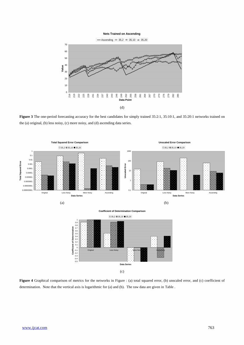
(d)

Figure 3 The one-period forecasting accuracy for the best candidates for simply trained 35:2:1, 35:10:1, and 35:20:1 networks trained on

the (a) original, (b) less noisy, (c) more noisy, and (d) ascending data series.

(a) (b)

(c)

Figure 4 Graphical comparison of metrics for the networks in Figure : (a) total squared error, (b) unscaled error, and (c) coefficient of

determination. Note that the vertical axis is logarithmic for (a) and (b). The raw data are given in Table .

Nets Trained on Ascending

0

10

20

30

40

50

60

70

21

6

21

9

22

2

22

5

22

8

23

1

23

4

23

7

24

0

24

3

24

6

24

9

25

2

25

5

25

8

26

1

26

4

26

7

27

0

27

3

27

6

27

9

28

2

28

5

Data Point

Valu

e

Ascending 35,2 35,10 35,20

Total Squared Error Comparison

0.000000001

0.00000001

0.0000001

0.000001

0.00001

0.0001

0.001

0.01

0.1

1

Original Less Noisy More Noisy Ascending

Data Series

To

tal

Sq

uare

d E

rro

r

35,2 35,10 35,20

Unscaled Error Comparison

0.1

1

10

100

1000


Data Series

Un

scale

d E

rro

r

35,2 35,10 35,20

Coefficient of Determination Comparison

-0.5

-0.4

-0.3

-0.2

-0.1

0

0.1

0.2

0.3

0.4

0.5

0.6

0.7

0.8

0.9

1


Data Series

Co

eff

icie

nt

of

Dete

rmin

ati

on

35,2 35,10 35,20

www.ijcat.com 764

Table 3 Parameters and metrics for the networks in Figure .

Arch. Candidate Data

Series

Ending

Learnin

g

Rate

Epochs

Total

Squared

Error

Unscaled

Error

Coeff. of

Determ.

(1 period)

Training

Time

(sec.)

35:2:1 b Original 0.1 100000 0.0035864 14.6705 0.9111 99

35:10:1 c Original 0.1 100000 3.02316e-006 0.386773 1.0000 286

35:20:1 a Original 0.1 100000 2.15442e-006 0.376312 1.0000 515

35:2:1 b Less Noisy 0.1 100000 0.0822801 84.8237 0.5201 99

35:10:1 committee (b) Less Noisy 0.1 100000 0.00341762 17.6535 0.9173 287

35:20:1 b Less Noisy 0.1 100000 0.00128001 10.8401 0.9453 531

35:2:1 b More

Noisy 0.1 100000 0.360209 203.893 -4.6748 100

35:10:1 a More

Noisy 0.1 100000 2.47609e-009 0.0166514 -0.0056 282

35:20:1 c More

Noisy 0.1 100000 0.000106478 3.65673 -1.5032 519

35:2:1 a Ascending 0.1 100000 0.023301 59.7174 0.4091 98

35:10:1 a Ascending 0.1 100000 0.000421792 8.67945 -0.3585 280

35:20:1 b Ascending 0.1 100000 0.000191954 5.87395 0.4154 529

9. REFERENCES

[1] M. Abdollahzade, A. Miranian, H. Hassani, and H.

Iranmanesh, “A new hybrid enhanced local linear

neuro-fuzzy model based on the optimized singular

spectrum analysis and its application for nonlinear

and chaotic time series forecasting,” Inf. Sci. (Ny)., vol. 295, pp. 107–125, 2015.

[2] J. Ares, J. A. Lara, D. Lizcano, and S. Suárez, “A

soft computing framework for classifying time series

based on fuzzy sets of events,” Inf. Sci. (Ny)., vol. 330, pp. 125–144, 2016.

[3] M.-Y. Chen and B.-T. Chen, “A hybrid fuzzy time

series model based on granular computing for stock

price forecasting,” Inf. Sci. (Ny)., vol. 294, pp. 227–241, 2015.

[4] T.-T. Chen and S.-J. Lee, “A weighted LS-SVM

based learning system for time series forecasting,”

Inf. Sci. (Ny)., vol. 299, pp. 99–116, 2015.

[5] Z. Chen, W. Zuo, Q. Hu, and L. Lin, “Kernel sparse

representation for time series classification,” Inf. Sci. (Ny)., vol. 292, pp. 15–26, 2015.

[6] S.-H. Cheng, S.-M. Chen, and W.-S. Jian, “Fuzzy

time series forecasting based on fuzzy logical

relationships and similarity measures,” Inf. Sci. (Ny)., vol. 327, pp. 272–287, 2016.

[7] H. Deng, G. Runger, E. Tuv, and M. Vladimir, “A

time series forest for classification and feature

extraction,” Inf. Sci. (Ny)., vol. 239, pp. 142–153,

2013.

[8] L. N. Ferreira and L. Zhao, “Time series clustering

via community detection in networks,” Inf. Sci. (Ny)., vol. 326, pp. 227–242, 2016.

[9] M. González, C. Bergmeir, I. Triguero, Y. Rodríguez,

and J. M. Benítez, “On the stopping criteria for k-

Nearest Neighbor in positive unlabeled time series

classification problems,” Inf. Sci. (Ny)., vol. 328, pp.

42–59, 2016.

[10] X. Huang, Y. Ye, L. Xiong, R. Y. K. Lau, N. Jiang,

and S. Wang, “Time series k-means: A new k-means

type smooth subspace clustering for time series data,” Inf. Sci. (Ny)., vol. 367–368, pp. 1–13, 2016.

[11] A. Kattan, S. Fatima, and M. Arif, “Time-series

event-based prediction: An unsupervised learning

framework based on genetic programming,” Inf. Sci. (Ny)., vol. 301, pp. 99–123, 2015.

[12] M. Krawczak and G. Szkatuła, “An approach to

dimensionality reduction in time series,” Inf. Sci. (Ny)., vol. 260, pp. 15–36, 2014.

[13] L. Liu, Y. Peng, S. Wang, M. Liu, and Z. Huang,

“Complex activity recognition using time series

pattern dictionary learned from ubiquitous sensors,” Inf. Sci. (Ny)., vol. 340, pp. 41–57, 2016.

[14] A. Marszałek and T. Burczyński, “Modeling and

forecasting financial time series with ordered fuzzy

candlesticks,” Inf. Sci. (Ny)., vol. 273, pp. 144–155,

2014.

[15] S. Miao, U. Vespier, R. Cachucho, M. Meeng, and A.

Knobbe, “Predefined pattern detection in large time series,” Inf. Sci. (Ny)., vol. 329, pp. 950–964, 2016.

www.ijcat.com 765

[16] V. Novák, I. Perfilieva, M. Holčapek, and V.

Kreinovich, “Filtering out high frequencies in time

series using F-transform,” Inf. Sci. (Ny)., vol. 274,

pp. 192–209, 2014.

[17] H. Pree, B. Herwig, T. Gruber, B. Sick, K. David,

and P. Lukowicz, “On general purpose time series

similarity measures and their use as kernel functions

in support vector machines,” Inf. Sci. (Ny)., vol. 281,

pp. 478–495, 2014.

[18] M. Pulido, P. Melin, and O. Castillo, “Particle swarm

optimization of ensemble neural networks with fuzzy

aggregation for time series prediction of the Mexican

Stock Exchange,” Inf. Sci. (Ny)., vol. 280, pp. 188–204, 2014.

[19] T. Xiong, Y. Bao, Z. Hu, and R. Chiong,

“Forecasting interval time series using a fully

complex-valued RBF neural network with DPSO and

PSO algorithms,” Inf. Sci. (Ny)., vol. 305, pp. 77–92, 2015.

[20] F. Ye, L. Zhang, D. Zhang, H. Fujita, and Z. Gong,

“A novel forecasting method based on multi-order

fuzzy time series and technical analysis,” Inf. Sci. (Ny)., vol. 367–368, pp. 41–57, 2016.

[21] H. Zhao, Z. Dong, T. Li, X. Wang, and C. Pang,

“Segmenting time series with connected lines under

maximum error bound,” Inf. Sci. (Ny)., vol. 345, pp.

1–8, 2016.

[22] S. Zhu, Q.-L. Han, and C. Zhang, “Investigating the

effects of time-delays on stochastic stability and

designing l1-gain controllers for positive discrete-

time Markov jump linear systems with time-delay,”

Inf. Sci. (Ny)., vol. 355, pp. 265–281, 2016.

Time Series Forecasting Using Novel Feature Extraction Algorithm and Multilayer Neural Network

Technology

Transcript of Time Series Forecasting Using Novel Feature Extraction Algorithm and Multilayer Neural Network