
Time Series Data Analysis Using R - Portland State Universityweb.pdx.edu/~crkl/ec572/TSAR-1.pdf ·...
31
Time Series Data Analysis Using R • Introduction to R • Getting Started - Using RStudio IDE – R 3.3.x – RStudio 1.0.xxx • On Line Data Resources – quantmod – Quandl 1 Time Series Data Analysis Using R
Transcript of Time Series Data Analysis Using R - Portland State Universityweb.pdx.edu/~crkl/ec572/TSAR-1.pdf ·...

Time Series Data Analysis Using R
• Introduction to R • Getting Started - Using RStudio IDE
– R 3.3.x
– RStudio 1.0.xxx
• On Line Data Resources
– quantmod
– Quandl
1 Time Series Data Analysis Using R

Time Series Data
• Economic Time Series Data – GDP, CPI, Oil Price, Climate Change – Interest Rates, Exchange Rates
• Financial Time Series Data
– S&P 500, VIX (Fear Index)
– International Stock Markets
• High Frequency Time Series
2 Time Series Data Analysis Using R
1 2{ } {..., , ,..., ,...}t ny y y y

Time Series Data
• Decomposition
– Additive Components
– Multiplicative Components
• Deterministic vs. Stochastic Trend (and/or Seasonality)
• Transformation
– Stationary vs. Non-stationary Time Series
• Box-Cox or Log -> Stationarity in the Variance
• Difference -> Stationarity in the Mean
3 Time Series Data Analysis Using R
log( ) ...t t t ty or y t x
log( )
t t t t
t t t t
y m s
y m s

Time Series Decomposition
• decompse – function (x, type = c("additive",
"multiplicative"), filter = NULL)
• stl – function (x, s.window, s.degree = 0, t.window =
NULL, t.degree = 1, l.window = nextodd(period),
l.degree = t.degree, s.jump =
ceiling(s.window/10), t.jump =
ceiling(t.window/10), l.jump =
ceiling(l.window/10), robust = FALSE, inner =
if (robust) 1 else 2, outer = if (robust) 15
else 0, na.action = na.fail)
Time Series Data Analysis Using R 4

Strategies for Time Series Analysis
• Data Exploration
– Using Graphs
• Hypothesis Testing
– Normality
– Stationarity
– Serial Correlation • Durbin-Watson
• Box-Pierce / Ljung-Box
• ACF/PACF
• Time Series Smoothing
– Exponential Smoothing
– Structural Time Series
• Model Estimation
– Regression Model
– ARIMA Model
– Dynamic Linear Model
Time Series Data Analysis Using R 5
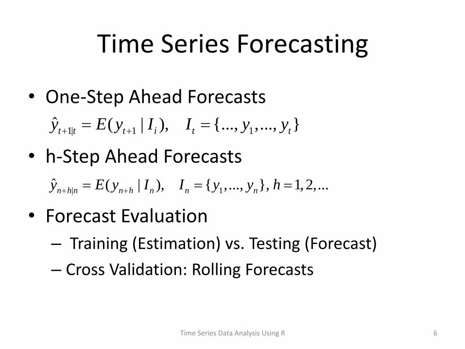
Time Series Forecasting
• One-Step Ahead Forecasts
• h-Step Ahead Forecasts
• Forecast Evaluation
– Training (Estimation) vs. Testing (Forecast)
– Cross Validation: Rolling Forecasts
Time Series Data Analysis Using R 6
1| 1 1ˆ ( | ), {..., ,..., }t t t i t ty E y I I y y
| 1ˆ ( | ), { ,..., }, 1,2,...n h n n h n n ny E y I I y y h
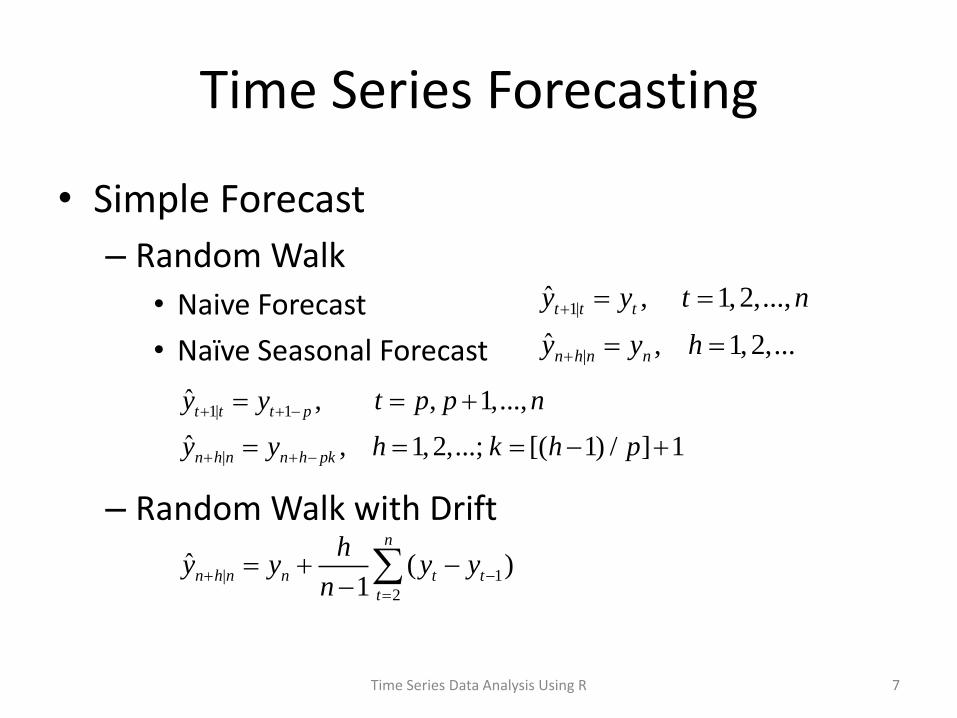
Time Series Forecasting
• Simple Forecast
– Random Walk
• Naive Forecast
• Naïve Seasonal Forecast
– Random Walk with Drift
7 Time Series Data Analysis Using R
1| 1
|
ˆ , , 1,...,
ˆ , 1,2,...; [( 1) / ] 1
t t t p
n h n n h pk
y y t p p n
y y h k h p
1|
|
ˆ , 1, 2,...,
ˆ , 1, 2,...
t t t
n h n n
y y t n
y y h
| 1
2
ˆ ( )1
n
n h n n t t
t
hy y y y
n
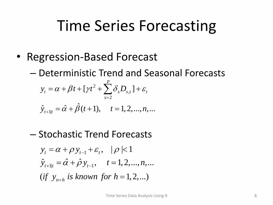
Time Series Forecasting
• Regression-Based Forecast
– Deterministic Trend and Seasonal Forecasts
– Stochastic Trend Forecasts
8 Time Series Data Analysis Using R
2
,
2
1|
[ ]
ˆˆˆ ( 1), 1,2,..., ,...
p
t s s t t
s
t t
y t t D
y t t n
1
1| 1
, | | 1
ˆ ˆˆ , 1, 2,..., ,...
( 1,2,...)
t t t
t t t
n h
y y
y y t n
if y is known for h

Time Series Forecasting
• One-Step Ahead Forecast Error
• Forecast Error Statistics
9 Time Series Data Analysis Using R
,..., 1|
,..., 1| 1
2
,..., 1|
2
,..., 1|
2
,..., 1| 1
ˆ(| |)
ˆ100 (| / |)
ˆ( )
ˆ( )
ˆ100 [( / ) ]
t p n t t
t p n t t t
t p n t t
t p n t t
t p n t t t
MAE mean
MAPE mean y
MSE mean
RMSE mean
RMSPE mean y
1| 1 1|ˆ ˆ , , 1,..., ( )t t t t ty y t p p n p seasonal period

Time Series Forecasting
• h-Step Ahead Forecast Error (if yn+h is known)
• Forecast Error Statistics
10 Time Series Data Analysis Using R
|
|
2
|
2
|
2
|
ˆ(| |)
ˆ100 (| / |)
ˆ( )
ˆ( )
ˆ100 [( / ) ]
h n h n
h n h n n h
h n h n
h n h n
h n h n n h
MAE mean
MAPE mean y
MSE mean
RMSE mean
RMSPE mean y
| |ˆ ˆ , 1,2,...n h n n h n h ny y h

Time Series Forecasting
• Using R Package forecast – rwf
• function (y, h = 10, drift = FALSE, level =
c(80, 95), fan = FALSE, lambda = NULL,
biasadj = FALSE, x = y)
– accuracy • function (f, x, test = NULL, d = NULL, D =
NULL)
Time Series Data Analysis Using R 11
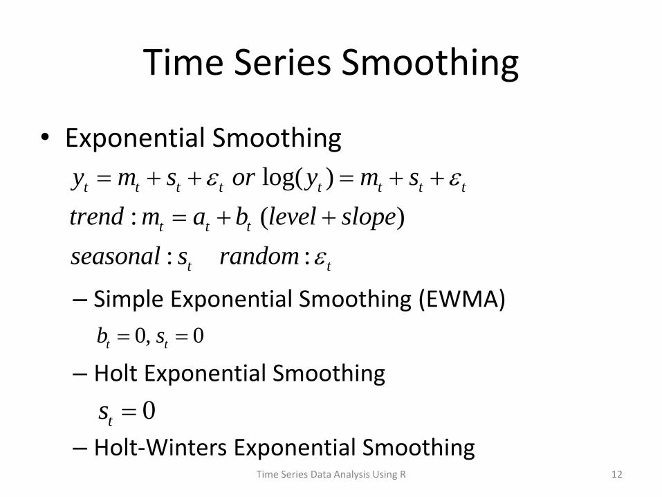
Time Series Smoothing
• Exponential Smoothing
– Simple Exponential Smoothing (EWMA)
– Holt Exponential Smoothing
– Holt-Winters Exponential Smoothing
12 Time Series Data Analysis Using R
log( )
: ( )
: :
t t t t t t t t
t t t
t t
y m s or y m s
trend m a b level slope
seasonal s random
0, 0t tb s
0ts
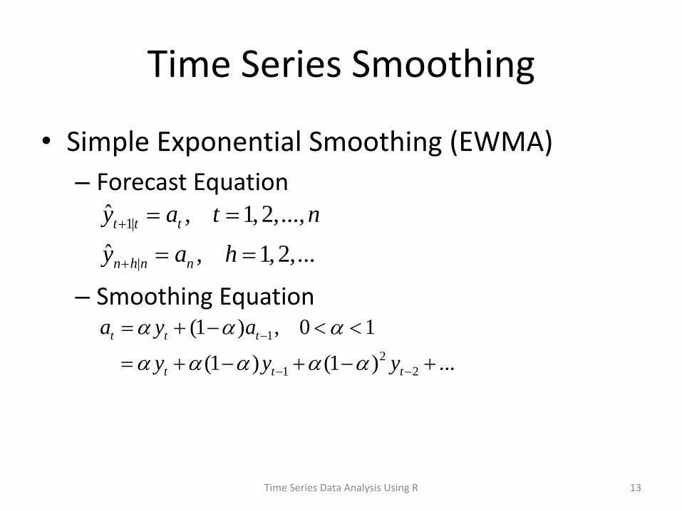
Time Series Smoothing
• Simple Exponential Smoothing (EWMA)
– Forecast Equation
– Smoothing Equation
13 Time Series Data Analysis Using R
1|
|
ˆ , 1,2,...,
ˆ , 1,2,...
t t t
n h n n
y a t n
y a h
1
2
1 2
(1 ) , 0 1
(1 ) (1 ) ...
t t t
t t t
a y a
y y y

Time Series Smoothing
• Simple Exponential Smoothing (EWMA)
– State Space Representation
– Model Estimation
14 Time Series Data Analysis Using R
2
0
1
1
ˆ min arg ,
, 1,2,...,
n
t
t
t t t
e with initials a
where e y a t n
1
1
( )
( )
t t t
t t t
y a e observation equation
a a e state equation

Time Series Smoothing
• Holt Exponential Smoothing
– Forecast Equation
– Smoothing Equation
15 Time Series Data Analysis Using R
1 1
1 1
(1 )( ), 0 1
( ) (1 ) , 0 1
t t t t
t t t t
a y a b
b a a b
1|
|
ˆ , 1,2,...,
ˆ , 1,2,...
t t t t
n h n n n
y a b t n
y a hb h

Time Series Smoothing
• Holt Exponential Smoothing
– State Space Representation
– Model Estimation
16 Time Series Data Analysis Using R
1 1
1 1
1
t t t t
t t t t
t t t
y a b e
a a b e
b b e
2
0 0( , ) 1
1 1
ˆˆ( , ) min arg , ( , )
( )
n
t
t
t t t t
e with initials a b
where e y a b

Time Series Smoothing
• Holt-Winters Exponential Smoothing
– Forecast Equation
– Smoothing Equation
17 Time Series Data Analysis Using R
1 1
1 1
( ) (1 )( ), 0 1
( ) (1 ) , 0 1
( ) (1 ) , 0 1
t t t p t t
t t t t
t t t t p
a y s a b
b a a b
s y a s
1| 1
| 1 [( 1)mod ]
|
ˆ , 1, 2,...,
ˆ , 1, 2,...
ˆ , 1, 2,...
t t t t t p
n h n n n n p h p
n h n n n n h p
y a b s t n
y a hb s h
y a hb s h p

Time Series Smoothing
• Holt-Winters Exponential Smoothing
– State Space Representation
18 Time Series Data Analysis Using R
1 1
1 1
1
(1 )
t t t t p t
t t t t
t t t
t t p t
y a b s e
a a b e
b b e
s s e
2
0 0 0 2 1( , , ) 1
1 1
ˆˆ ˆ( , , ) min arg , ( , , ,..., , )
( )
n
t p p
t
t t t t t p
e with initials a b s s s
where e y a b s

Time Series Smoothing
• One-Step Ahead Forecast at t = p, p+1,…
19 Time Series Data Analysis Using R
1| 1
1| 1
2| 1 1 1 2
2 |2 1 2 1 2 1
2 1|2 2 2 1
| 1 1 1 1
ˆ
ˆ
ˆ
...
ˆ
ˆ
...
ˆ
t t t t t p
p p p p
p p p p
p p p p p
p p p p p
n n n n n p
y a b s
y a b s
y a b s
y a b s
y a b s
y a b s
1|0 0 0 1
2|1 1 1 2
| 1 1 1 0
ˆ
ˆ
...
ˆ
p
p
p p p p
Initialization
y a b s
y a b s
y a b s
1| 1 1|ˆ ˆ
, 1,...,
t t t t t
Forecast Error
y y
t p p n
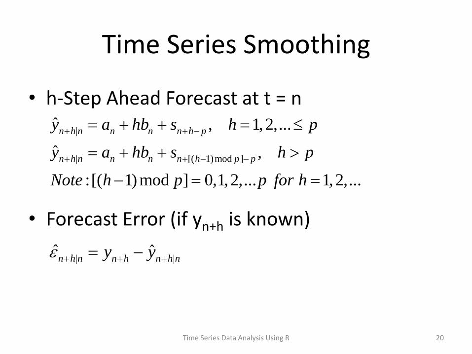
Time Series Smoothing
• h-Step Ahead Forecast at t = n
• Forecast Error (if yn+h is known)
20 Time Series Data Analysis Using R
|
| [( 1)mod ]
ˆ , 1, 2,...
ˆ ,
:[( 1)mod ] 0,1,2,... 1, 2,...
n h n n n n h p
n h n n n n h p p
y a hb s h p
y a hb s h p
Note h p p for h
| |ˆ ˆn h n n h n h ny y

Time Series Data Analysis Using R 21
| 1 [( 1)mod ]
1| 1
2| 2
|
1| 1
1| 2
|
ˆ
ˆ1:
ˆ2 : 2
...
ˆ:
ˆ1: ( 1)
ˆ2 : ( 2)
...
ˆ2 : 2
..
n h n n n n p h p
n n n n n p
n n n n n p
n p n n n n
n p n n n n p
n p n n n n p
n h n n n n
y a hb s
h y a b s
h y a b s
h p y a pb s
h p y a p b s
h p y a p b s
n p y a pb s
2 |2 1 2 1 2 1
2 1|2 2 2 1
.
ˆ
ˆ
...
p p p p p
p p p p p
y a b s
y a b s

Time Series Smoothing
• HoltWinters – function (x, alpha = NULL, beta = NULL, gamma =
NULL, seasonal = c("additive",
"multiplicative"), start.periods = 2, l.start =
NULL, b.start = NULL, s.start = NULL,
optim.start = c(alpha = 0.3, beta = 0.1, gamma
= 0.1), optim.control = list())
• Predict.HoltWinters – predict(object, n.ahead = 1,
prediction.interval = FALSE, level = 0.95, ...)
Time Series Data Analysis Using R 22

Time Series Smoothing
• Using R Package forecast:
• ets – function (y, model = "ZZZ", damped = NULL,
alpha = NULL, beta = NULL, gamma = NULL, phi =
NULL, additive.only = FALSE, lambda = NULL,
biasadj = FALSE, lower = c(rep(1e-04, 3), 0.8),
upper = c(rep(0.9999, 3), 0.98), opt.crit =
c("lik", "amse", "mse", "sigma", "mae"), nmse =
3, bounds = c("both", "usual", "admissible"),
ic = c("aicc", "aic", "bic"), restrict = TRUE,
allow.multiplicative.trend = FALSE,
use.initial.values = FALSE, ...)
Time Series Data Analysis Using R 23

Time Series Smoothing
• Using R Package forecast:
• forecast – function(object,
h=ifelse(frequency(object$x)>1,
2*frequency(object$x),10), level=c(80,95),
fan=FALSE, lambda=NULL, biasadj=FALSE,...)
Time Series Data Analysis Using R 24

Structural Time Series Model
• Linear Gaussian State Space Model
– Measurement (Observation) Equation
– State Equations
Time Series Data Analysis Using R 25
1 1
1
1 1...
t t t t
t t t
t t t p t
a a b
b b
s s s
2
2
2
~ (0, )
~ (0, )
~ (0, )
t
t
t
N
N
N
2~ (0, )t t t t ty a s N

Structural Time Series Model
• Special Cases
– Non-Seasonal (or Local Linear Trend) Model
– Local Level Model
Time Series Data Analysis Using R 26
1 1
1
t t t
t t t t
t t t
y a
a a b
b b
2
2
2
~ (0, )
~ (0, )
~ (0, )
t
t
t
N
N
N
1
t t t
t t t
y a
a a
2
2
~ (0, )
~ (0, )
t
t
N
N

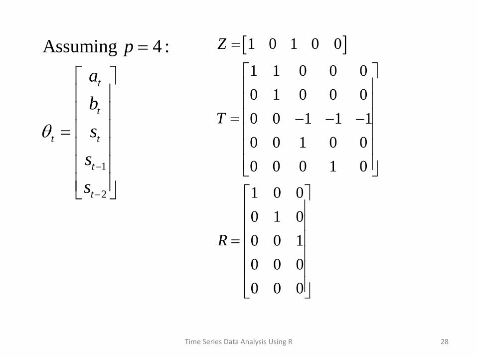
Structural Time Series Model
• Linear Gaussian State Space Model
– Matrix Representation
Time Series Data Analysis Using R 27
2
1
0 0 0
~ (0, )
~ (0, )
~ ( , )
t t t t
t t t t
y Z N
T R N V
N C P
2
2
2
0 0
, 0 0
0 0
t
t t
t
V
Time Series Data Analysis Using R 28
1 0 1 0 0
1 1 0 0 0
0 1 0 0 0
0 0 1 1 1
0 0 1 0 0
0 0 0 1 0
1 0 0
0 1 0
0 0 1
0 0 0
0 0 0
Z
T
R
1
2
Assuming 4 :
t
t
t t
t
t
p
a
b
s
s
s

Structural Time Series Model
• StrucTS – function (x, type = c("level", "trend", "BSM"),
init = NULL, fixed = NULL, optim.control =
NULL)
Time Series Data Analysis Using R 29

Example 1
• GDP and GDP Growth
– GDP Quarterly Time Series
• Trend, Seasonality
– GDP Growth
• Simple vs Compound Growth Rate
• Quarterly Growth vs Annual Growth
– Time Series Decomposition
– Smoothing and Forecasting
30 Time Series Data Analysis Using R

Example 2
• Standard and Poor’s 500 Stock Index
– High Frequency Daily Index
– Monthly Index Time Series
• Trend, Seasonality
– Monthly Log-Return and Volatility
– Time Series Decomposition
– Exponential Smoothing and Forecasting
31 Time Series Data Analysis Using R