Time Reversal inRandomly Layered Media

Jean-Pierre Fouque

North Carolina State University

CIRM, Marseille

September 7, 2005

1

Reference:

Wave Propagation and Time Reversal in

Randomly Layered Media

To appear: Springer 2006

J.P. Fouque, J. Garnier, G. Papanicolaou, K. Solna

Papers at:

http://www.math.ncsu.edu/˜fouque

2

WARNING!

George Papanicolaou presented a qualitative, model

independent, analysis for applications to imaging.

Here we present a quantitative, model dependent,

analysis for applications to destruction!

3

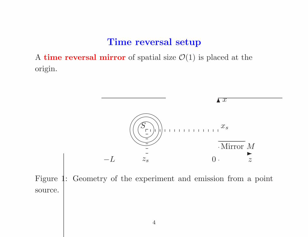
Time reversal setup

A time reversal mirror of spatial size O(1) is placed at the

origin.

-

6

−L 0 z

x

xs

zs

S

Mirror M

��������

&%'$

Figure 1: Geometry of the experiment and emission from a point

source.

4

Internal source problem

Acoustic equations in three dimensions:

ρ∂~u

∂t+ ∇p = ~F,

1

K

∂p

∂t+ ∇.~u = 0,

Randomly layered matched medium:

ρ ≡ ρ,1

K=

1

K

(1 + ν

( z

ε2

))if z ∈ [−L, 0],

1

Kif z ∈ (−∞,−L) ∪ (0,∞) ,

An internal source at (xs, zs), zs ≤ 0, −→ short pulse at time ts:

~F(t,x, z) = ε2~f

(t − ts

ε,x − xs

)δ(z − zs) ,

5

Field generated at the surface by an internal point source

ps(t,x) =1

(2πε)3

∫ √I(κ)

2a(ω, κ, 0)e−

iωε

(t−κ.x)ω2dωdκ,

us(t,x) =1

(2πε)3

∫1

2√

I(κ)a(ω, κ, 0)e−

iωε

(t−κ.x)ω2dωdκ,

vs(t,x) =1

(2πε)3

∫ √I(κ)

2ρκa(ω, κ, 0)e−

iωε

(t−κ.x)ω2dωdκ,

where ~us = (vs, us) and

a(ω, κ, 0) is the the right going mode (ω, κ) at the surface z = 0.

I(κ) = ρc(κ), c(κ) =c√

1 − c2κ2, c =

√K/ρ.

6

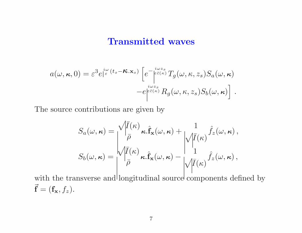
Transmitted waves

a(ω, κ, 0) = ε3eiωε

(ts−κ.xs)[e−

iωzsεc(κ) Tg(ω, κ, zs)Sa(ω, κ)

−eiωzsεc(κ) Rg(ω, κ, zs)Sb(ω, κ)

].

The source contributions are given by

Sa(ω, κ) =

√I(κ)

ρκ.fx(ω, κ) +

1√I(κ)

fz(ω, κ) ,

Sb(ω, κ) =

√I(κ)

ρκ.fx(ω, κ) − 1√

I(κ)fz(ω, κ) ,

with the transverse and longitudinal source components defined by~f = (fx, fz).

7

Reflection and transmission coefficients and their adjoints

-−L 0z

�T(ω,κ)(−L, z)

-0 � 1

-R(ω,κ)(−L, z)

-−L 0z

�R(ω,κ)(z,0)

-1 � 0

-T(ω,κ)(z,0)

8

Generalized coefficients Rg and Tg

Rg(ω, κ, z) = T(ω,κ)(z, 0)R(ω,κ)(−L, z)

∞∑

k=0

(R(ω,κ)(z, 0)R(ω,κ)(−L, z)

)k

=T(ω,κ)(z, 0)R(ω,κ)(−L, z)

1 − R(ω,κ)(z, 0)R(ω,κ)(−L, z),

Tg(ω, κ, z) = T(ω,κ)(z, 0)∞∑

k=0

(R(ω,κ)(z, 0)R(ω,κ)(−L, z)

)k

=T(ω,κ)(z, 0)

1 − R(ω,κ)(z, 0)R(ω,κ)(−L, z).

9

Field generated in the medium by a surface point source

Case of a source located at the surface zs = 0 with xs = 0:

~F(t,x, z) = ε2~g

(t − ts

ε,x

)δ(z)

u(t,x, z) =−1

(2πε)3

∫1

2√

I(κ)Sb(ω, κ)

[Rg(ω, κ, z)e

iωzεc(κ)

+Tg(ω, κ, z)e−iωz

εc(κ)

]e−

iωε

(t−κ.x)ω2dωdκ.

Sb(ω, κ) =

√I(κ)

ρκ.gx(ω, κ) − 1√

I(κ)gz(ω, κ).

10

Time reversal with an active point source

(Ref: Time Reversal Super Resolution in Randomly Layered Media

Fouque-Garnier-Sølna, submitted 2005.)

Source at (xs, zs), zs < 0, emits a short pulse:

~F(t,x, z) = ε2~f

(t − ts

ε

)δ(x− xs)δ(z − zs)

TR Mirror at the surface: M = {(x, z),x ∈ D(0), z = 0}, records

during some time interval centered at t = 0, for a duration t1 > 0.

A piece of the recorded signal is clipped using a cut-off function G1

with support in [−t1/2, t1/2]:

~urec(t,x) = ~us(t,x)G1(t)G2 (x) , G2(x) = 1D(x).

Time Reversal:

~FTR(t,x, z) = ~fTR(t,x)δ(z), ~fTR(t,x) = ρc~urec(−t,x),

11

New source modes generated by TR

fTR,x(ω, κ) =ρc

(2πε)3

∫ √I(κ′)

2ρκ′a(ω′, κ

′, 0)G1

(ω − ω′

ε

)

×G2

(ωκ + ω′

κ′

ε

)ω′2dω′dκ

′,

fTR,z(ω, κ) =ρc

(2πε)3

∫1

2√

I(κ′)a(ω′, κ

′, 0)G1

(ω − ω′

ε

)

×G2

(ωκ + ω′

κ′

ε

)ω′2dω′dκ

′,

where a(ω, κ, 0) is given above by

a(ω, κ, 0) = ε3eiωε

(ts−κ.xs)[e−

iωzsεc(κ) Tg(ω, κ, zs)Sa(ω, κ)

−eiωzsεc(κ) Rg(ω, κ, zs)Sb(ω, κ)

]

12

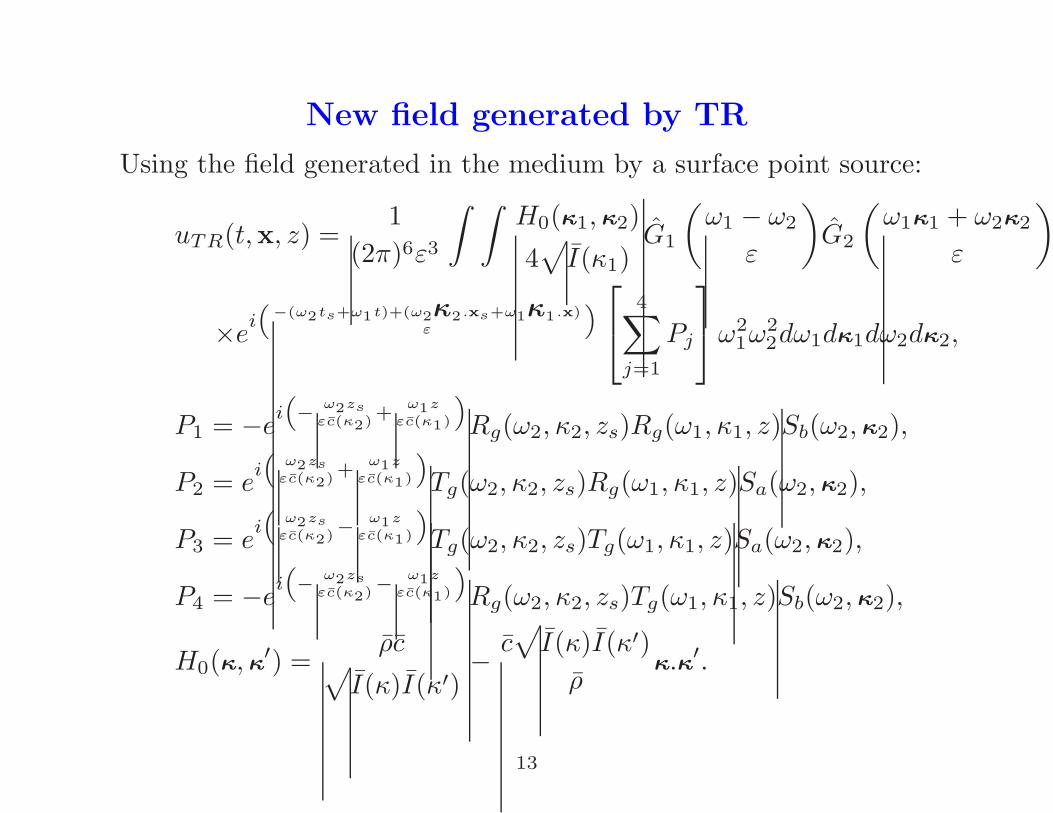
New field generated by TR

Using the field generated in the medium by a surface point source:

uTR(t,x, z) =1

(2π)6ε3

∫ ∫H0(κ1, κ2)

4√

I(κ1)G1

(ω1 − ω2

ε

)G2

(ω1κ1 + ω2κ2

ε

)

×ei“

−(ω2ts+ω1t)+(ω2κ2.xs+ω1κ1.x)ε

”

4∑

j=1

Pj

ω2

1ω22dω1dκ1dω2dκ2,

P1 = −ei“

−ω2zs

εc(κ2)+ω1z

εc(κ1)

”

Rg(ω2, κ2, zs)Rg(ω1, κ1, z)Sb(ω2, κ2),

P2 = ei“

ω2zsεc(κ2)

+ω1z

εc(κ1)

”

Tg(ω2, κ2, zs)Rg(ω1, κ1, z)Sa(ω2, κ2),

P3 = ei“

ω2zsεc(κ2)−

ω1z

εc(κ1)

”

Tg(ω2, κ2, zs)Tg(ω1, κ1, z)Sa(ω2, κ2),

P4 = −ei“

−ω2zs

εc(κ2)−ω1z

εc(κ1)

”

Rg(ω2, κ2, zs)Tg(ω1, κ1, z)Sb(ω2, κ2),

H0(κ, κ′) =

ρc√I(κ)I(κ′)

− c√

I(κ)I(κ′)

ρκ.κ′.

13

Nearby frequencies and slownesses

ω1 = ω + εh/2, ω2 = ω − εh/2, κ1 = κ + ελ/2, κ2 = −κ + ελ/2,

uTR(t,x, z) ≈ 1

(2π)6

∫ ∫H0(κ,−κ)

4√

I(κ)G1(h)G2 (hκ + ωλ)

4∑

j=1

Pj

×eiωε

(−(ts+t)+κ.(x−xs))eih2 (ts−t+κ.(x+xs))+ iω

2 λ.(x+xs)ω4dωdhdκdλ,

P1 = −e−iω

ε

zs−z

c(κ) eih2

zs+z

c(κ) − iω2 λ.κc(κ)(zs+z) RgRg Sb(ω,−κ),

P2 = eiωε

zs+z

c(κ) e−ih2

zs−z

c(κ) + iω2 λ.κc(κ)(zs−z) TgRg Sa(ω,−κ),

P3 = eiωε

zs−z

c(κ) e−ih2

zs+z

c(κ)+ iω

2 λ.κc(κ)(zs+z) TgTg Sa(ω,−κ),

P4 = −e−iωε

zs+z

c(κ) eih2

zs−z

c(κ) − iω2 λ.κc(κ)(zs−z) RgTg Sb(ω,−κ),

with complex conjugate, evaluated at (ω − εh/2,−κ + ελ/2, zs),

without complex conjugate, evaluated at (ω + εh/2, κ + ελ/2, z).

14

Time reversal in a homogeneous medium

In the deterministic case ν ≡ 0:

Rg = 0, and Tg = 1 =⇒

uTR(t,x, z) =1

(2π)6

∫ ∫c(κ)

4c√

I(κ)Sa(ω,−κ)G1(h)G2 (hκ + ωλ)

×eiφ

ε eih2 (ts−t+κ.(x+xs)− zs+z

c(κ) )+ iω2 (λ.(x+xs)+λ.κc(κ)(zs+z))ω4dωdhdκdλ,

where the rapid phase is

φ = ω

(−(ts + t) + κ.(x − xs) +

zs − z

c(κ)

)

15

Stationary phase

Three cases depending on the observation time t and the

observation point M = (x, z).

• If t < −ts, then there exists one stationary map given by κ = κs

and any ω, with

κs = −1

c

x − xs√|z − zs|2 + |x − xs|2

= −1

c

x − xs

SM,

if and only if the observation point M satisfies z > zs and

SM = c|t + ts|. The stationary phase method gives that

uTR(t,x, z) is of order ε.

• If t > −ts, then there exists one stationary map given by

κ = −κs and any ω, if and only if the observation point M satisfies

z < zs and SM = c(t + ts). Again the stationary phase method

gives that uTR(t,x, z) is of order ε.

16

Critical time

• If t = −ts, the critical time, there exists one stationary map if

and only if x = xs and z = zs, and uTR(t,x, z) is of order one.

We consider the refocused pulse locally:

t = −ts + εT, x = xs + εX, and z = zs + εZ.

uTR(t,x, z) =1

(2π)6

∫ ∫c(κ)

4c√

I(κ)Sa(ω,−κ)G1(h)G2 (hκ + ωλ)

×eiω(−T+κ.X− Zc(κ) )eih(ts+κ.xs−

zsc(κ) )+iω(λ.xs+λ.κc(κ)zs)ω4dωdhdκdλ

Apply the change of variables λ 7→ k = ωλ + hκ and integrate with

respect to k and h:

uTR(t,x, z) =1

(2π)3

∫ ∫c(κ)

4c√

I(κ)G1

(ts − zs

c(κ)

c2

)G2 (xs + κc(κ)zs)

×Sa(ω,−κ)eiω(−T+κ.X− Zc(κ) )ω2dωdκ.

17

Qualitative refocusing

t < −ts t = −ts t > −ts

−1 0 1 2 3 4 5 6−5

−4

−3

−2

−1

0

1

S

O

x

z

−1 0 1 2 3 4 5 6−5

−4

−3

−2

−1

0

1

S

O

xz

−1 0 1 2 3 4 5 6−5

−4

−3

−2

−1

0

1

S

O

x

z

amplitude O(ε) amplitude O(1) amplitude O(ε)

Pulse refocusing in homogeneous medium. The focal spot

size depends on the numerical aperture which measures the angular

diversity of the refocused waves which participate in the refocusing.

18

Cones of aperture

~e1 =1

OS

( −zs0xs

), ~e2 =

(010

), ~e3 =

1

OS

( xs0zs

),

0 2 4−5

−4

−3

−2

−1

0

1

∆φ1

S

O−a/2 a/2 xs

zs

e3

e1

x

z

−4 −2 0 2 4

−6

−4

−2

0

∆φ2

O−a/2 a/2

S

e3

e2

y

19

Spot sizes - Rayleigh resolution formula

~f(t) = ~f0

(t

Tw

)cos(ω0t), ω0Tw ≫ 1, |zs| ≫ a, G2(x) = g2

(x

a

)

|uTR(t,x, z)| =

C

∣∣∣∣∣~OS.~f0OS

(− T

Tw+

(X, Z).~e3

cTw

)∣∣∣∣∣

∣∣∣∣g2

(ω0a|zs|cOS2

(X, Z).~e1,ω0a

cOS(X, Z).~e2

)∣∣∣∣ .

- In the ~e3-direction: R3 = cTw

- In the ~e2-direction: R2 = λ0OS/a = λ0/∆φ2, λ0 = 2πc/ω0

- In the ~e1-direction: R1 = λ0OS2/(a|zs|) = λ0/∆φ1

20

−2 −1 0 1 2

−2

−1.5

−1

−0.5

0

0.5

1

1.5

2

(x−xs)/D⊥

(z−

z s)/D

⊥

In the plane (~e1,~e3): the spot shape is a sinc with radius D⊥ = λ0/∆φ1

in the ~e1 direction, a Gaussian with radius cTw in the ~e3 direction, and

a sinc with radius λ0/∆φ2 in the ~e2 orthogonal direction (not shown).

21

Random Medium

Consider the P3 term in the longitudinal velocity uTR:

The generalized transmission coefficient depends only on the

modulus of the slowness vector κ, so that:

u(3)TR(t,x, z) =

1

(2π)6

∫ ∫c(κ)

4c√

I(κ)Sa(ω,−κ)G1(h)G2 (hκ + ωλ)

×Tg (ω − εh/2, | − κ + ελ/2|, zs)Tg (ω + εh/2, |κ + ελ/2|, z)

×eiφ

ε eih2 (ts−t+κ.(x+xs)− zs+z

c(κ) )+ iω2 (λ.(x+xs)+λ.κc(κ)(zs+z))ω4dωdhdκdλ,

where the rapid phase is

φ = ω

(−(ts + t) + κ.(x − xs) +

zs − z

c(κ)

)

Stationary phase + asymptotic behavior of TgTg?

22

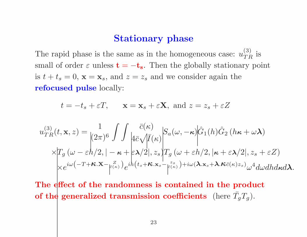
Stationary phase

The rapid phase is the same as in the homogeneous case: u(3)TR is

small of order ε unless t = −ts. Then the globally stationary point

is t + ts = 0, x = xs, and z = zs and we consider again the

refocused pulse locally:

t = −ts + εT, x = xs + εX, and z = zs + εZ

u(3)TR(t,x, z) =

1

(2π)6

∫ ∫c(κ)

4c√

I(κ)Sa(ω,−κ)G1(h)G2 (hκ + ωλ)

×Tg (ω − εh/2, | − κ + ελ/2|, zs)Tg (ω + εh/2, |κ + ελ/2|, zs + εZ)

×eiω(−T+κ.X− Zc(κ) )eih(ts+κ.xs−

zsc(κ) )+iω(λ.xs+λ.κc(κ)zs)ω4dωdhdκdλ.

The effect of the randomness is contained in the product

of the generalized transmission coefficients (here TgTg).

23

Expectation of the refocused pulse

The generalized coefficient Tg is given as a series of powers of

reflection/transmission coefficients and their adjoints. A careful

asymptotic analysis leads to:

E

[Tg (ω − εh/2, κ − εl/2, zs)Tg (ω + εh/2, κ + εl/2, zs + εZ)

]

ε→0−→∫

ei[h−ωlc(κ)2κ]τW(−)g (ω, κ, τ) dτ

where

W(−)g (ω, κ, τ) =

∞∑

n=0

[Wn(·, ω, κ,−L, zs) ∗W(T )

n (·, ω, κ, zs, 0)](τ),

and the Wn’s and W(T )n ’s are solutions of systems of transport

equations −→

24

Transport equations

∂Wp

∂z+

2p

c(κ)

∂Wp

∂τ=

p2

L(κ)loc

(Wp+1 + Wp−1 − 2Wp)

Wp(τ, ω, κ, z0, z = z0) = 10(p)δ(τ)

∂W(T )p

∂z+

2p

c(κ)

∂W(T )p

∂τ=

1

L(κ)loc

((p + 1)2W(T )

p+1 + p2W(T )p−1 − (p2 + (p + 1)2)W(T )

p

W(T )p (τ, ω, κ, z0, z = z0) = 10(p)δ(τ)

The localization length L(κ)loc is defined by

L(κ)loc =

c2

c(κ)24c2

γω2=

c2

c(κ)2Lloc, γ =

∫ ∞

−∞

E[ν(0)ν(z)]dz.

25

Expectation of the refocused pulse in the limit ε → 0

E[u(3)TR(t,x, z)] =

1

(2π)3

∫ ∫c(κ)

4c√

I(κ)Sa(ω,−κ)G1

(ts − zs

c(κ)

c2+

τ c(κ)2

c2

)

×G2

(xs + κc(κ)zs − c(κ)2κτ

)W(−)

g (ω, κ, τ)eiω(−T+κ.X− Zc(κ) )ω2dωdκdτ.

In the limit ε → 0, the cross moments of Rg and Tg are zero, so

that the contributions of the P2 and P4 terms vanish.

E[u(1)TR(t,x, z)] = − 1

(2π)3

∫ ∫c(κ)

4c√

I(κ)Sb(ω,−κ)G1

(ts − zs

c(κ)

c2+

τ c(κ)2

c2

)

×G2

(xs + κc(κ)zs − c(κ)2κτ

)W(+)

g (ω, κ, τ)eiω(−T+κ.X+ Zc(κ) )ω2dωdκdτ,

where

W(+)g (ω, κ, τ) =

∞∑

n=0

[Wn+1(·, ω, κ,−L, zs) ∗ W(T )

n (·, ω, κ, zs, 0)](τ).

26

Stable refocusing at the source

A Higher moments analysis shows that uTR converges to a

deterministic limit (given by the limit of its expectation).

uTR(t,x, z) −→ 0 unless (t,x, z) = (−ts,xs, zs), in which case

uTR(−ts + εT,xs + εX, zs + εZ) −→ UTR(T,X, Z)

where UTR is the deterministic pulse shape

1

(2π)3

∫K+(ω, κ)

[c(κ)κ.fx(ω) + fz(ω)

]eiω(−T+κ.X+ Z

c(κ) )ω2dωdκ

+1

(2π)3

∫K−(ω, κ)

[−c(κ)κ.fx(ω) + fz(ω)

]eiω(−T+κ.X− Z

c(κ) )ω2dωdκ,

and the refocusing kernels are given by

K(±)(ω, κ) =1

4cρ

∫G1

(ts − zs

c(κ)

c2+

τ c(κ)2

c2

)

×G2

(xs + κc(κ)zs − c(κ)2κτ

)W(±)

g (ω, κ, τ) dτ

27

Super Resolution

In order to be more quantitative we consider the case

|zs| ≪ Lloc ≪ L, with Lloc = 4c2/(γω20) (regime where a coherent

wave front remains).

W0(ω, κ, τ,−L, zs) = δ(τ),

W1(ω, κ, τ,−L, zs) =c(κ)3

2c2Lloc

1(1 + c(κ)3τ

2c2Lloc

)2 1[0,∞)(τ),

W2(ω, κ, τ,−L, zs) =c(κ)6τ

2c4L2loc

1(1 + c(κ)3τ

2c2Lloc

)3 1[0,∞)(τ),

W(T )0 (ω, κ, τ, zs, 0) = exp

(− c(κ)2

c2

|zs|Lloc

)δ(τ) ≃

[1 − c(κ)2

c2

|zs|Lloc

]δ(τ),

W(T )1 (ω, κ, τ, zs, 0) =

c(κ)3

2c2Lloc1[0,2|zs|/c(κ)](τ).

28

Coherent and incoherent contributions

W(+)g (ω, κ, τ) =

c(κ)3

2c2Lloc

1(1 + c(κ)3τ

2c2Lloc

)2 − |zs|Lloc

c(κ)5

2c4Lloc

1 − c(κ)3τ2c2Lloc(

1 + c(κ)3τ2c2Lloc

)3 ,

W(−)g (ω, κ, τ) = exp

(− c(κ)2

c2

|zs|Lloc

)δ(τ) +

|zs|Lloc

c(κ)5

2c4Lloc

1(1 + c(κ)3τ

2c2Lloc

)2 .

The first term in W(−)g corresponds to the contribution of the

coherent wave front.

The other terms are the contributions of the incoherent waves.

Note that the first term W(+)g has a mass of the same order as the

contribution of the coherent front.

29

Time reversal of the front.

The function G1 is of the form [T0 − δ, T0 + δ] with ε ≪ δ ≪ 1 and

T0 =OS

c+ ts

which corresponds to the arrival time at the mirror of the

front wave emitted by the source.

Normalized focal spot:

UTR(T,X, Z) ≃ exp

(− OS2

|zs|Lloc

) ~OS.~f0OS

(− T

Tw+

(X, Z).~e3

cTw

)

×g2

(ω0∆φ1

c(X, Z).~e1,

ω0∆φ2

c(X, Z).~e2

)

where the ∆φj ’s are as in the homogeneous case. This shows that

the focal spot shape is the same as in the homogeneous

case. The only difference is a slight reduction of the amplitude due

to the decay of the coherent energy.

30

Time reversal of the coda

Now, let us assume that we record some part of the long

incoherent waves. This means that G1(t) = 1[T1,T2](t) where

T0 < T1 < T2.

We also assume the offset xs > 0 and we introduce the angles

0 < θ1 < θ2 < π/2 which define the cone of aperture generated

by the incoherent scattered waves:

31

0 2 4 6 8

−6

−4

−2

0∆φ

1

∆θ1

S

O−a/2 a/2 xs

zs e

3

e1

x

z

(~e1,~e3)-section

32

−2 −1 0 1 2−10

−8

−6

−4

−2

0

∆φ2

∆θ2

O−a/2 a/2

S

e3

e2

y

(~e2,~e3)-section

33

Focal spot

Suppose |zs| ≪ Lloc and 0 < xs ≪ Lloc.

Write θ1 = θ − ∆θ/2 and θ2 = θ + ∆θ/2, and define

~w1 =

(sin θ

0− cos θ

), ~w2 =

(010

), ~w3 =

(cos θ

0sin θ

),

Then the shape of the refocused field divided by the maximal

amplitude (a2ω20)/(32π2ρc3Llocxs sin2(θ)) is equal to:

|UTR(T,X, Z)| ≃∣∣∣∣g2

(ω0∆θ1

c(X, Z).~w1,

ω0∆θ2

c(X, Z).~w2

)∣∣∣∣

×∣∣∣∣sinc

(ω0∆θ

2c(X, Z).~w1

)∣∣∣∣∣∣∣∣~w3.~f0

(− T

Tw+

(X, Z).~w3

cTw

)∣∣∣∣ .

where

∆θ1 =a

xs tan θ, ∆θ2 =

a cos θ

xs

34

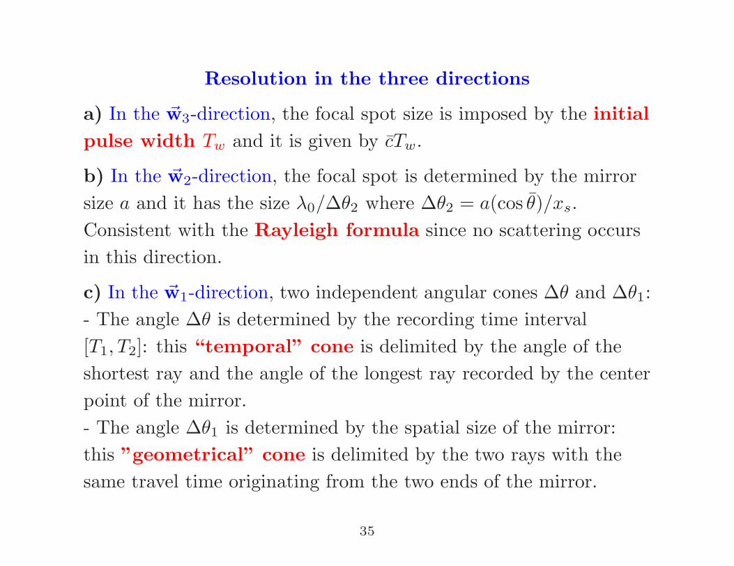
Resolution in the three directions

a) In the ~w3-direction, the focal spot size is imposed by the initial

pulse width Tw and it is given by cTw.

b) In the ~w2-direction, the focal spot is determined by the mirror

size a and it has the size λ0/∆θ2 where ∆θ2 = a(cos θ)/xs.

Consistent with the Rayleigh formula since no scattering occurs

in this direction.

c) In the ~w1-direction, two independent angular cones ∆θ and ∆θ1:

- The angle ∆θ is determined by the recording time interval

[T1, T2]: this “temporal” cone is delimited by the angle of the

shortest ray and the angle of the longest ray recorded by the center

point of the mirror.

- The angle ∆θ1 is determined by the spatial size of the mirror:

this ”geometrical” cone is delimited by the two rays with the

same travel time originating from the two ends of the mirror.

35

1. Only a very short piece of coda is recorded

∆θ ≪ ∆θ1 ≪ 1

|UTR(T,X, Z)| ≃∣∣∣∣g2

(ω0∆θ1

c(X, Z).~w1,

ω0∆θ2

c(X, Z).~w2

)∣∣∣∣

×∣∣∣∣~w3.~f0

(− T

Tw+

(X, Z).~w3

cTw

)∣∣∣∣

Geometrical angular diversity of the refocused waves in qualitative

agreement with the Rayleigh resolution formula. More

quantitatively, if we record a piece of the coda just after the front,

meaning that T1, T2 are close to T0, then θ = arccos(xs/OS) and

the focal spot size is λ0|zs|/a. Recall that the focal spot size

generated by the front is given by λ0OS2/(a|zs|).The random medium enables to correct for the offset xs.

36

2. A long piece of coda is recorded

∆θ1 ≪ ∆θ ≪ 1

|UTR(T,X, Z)| ≃∣∣∣∣g2

(0,

ω0∆θ2

c(X, Z).~w2

)∣∣∣∣∣∣∣∣sinc

(ω0∆θ

2c(X, Z).~w1

)∣∣∣∣

×∣∣∣∣~w3.~f0

(− T

Tw+

(X, Z).~w3

cTw

)∣∣∣∣

The focal spot size is λ0/∆θ as soon as ∆θ > a/OS. This size is

determined by the angular diversity of the refocused incoherent

waves and it is much smaller than the prediction of the

Rayleigh resolution formula. It is actually of the order of the

diffraction limit if T2 − T1 ≥ c/xs, so that ∆θ ∼ 1 with

(∆θ)max = π/2 − θ0. Recording a long coda allows us to enhance

dramatically the effective aperture of the mirror thanks to the

multiple scattering in the random medium.

37

Et Voila! The Raleigh resolution!

−2 −1 0 1 2

−2

−1.5

−1

−0.5

0

0.5

1

1.5

2

(x−xs)/D⊥

(z−

z s)/D

⊥

−2 −1 0 1

−2

−1.5

−1

−0.5

0

0.5

1

1.5

2

(x−xs)/D⊥

(z−

z s)/D

⊥

38

Left picture: Pulse shape generated by the refocusing of the incoherent

waves in the plane (~w1, ~w3). Here a = 0.33, zs = −3, xs = 4 (OS = 5),

ts = 0 (cT0 = 5), cT1 = 6, cT2 = 8 so that tan θ = 1.38, ∆φ1 = 0.04,

∆θ1 = 0.06 and ∆θ = 0.2. As a result the spot shape is a sinc function

with radius D⊥/5 where D⊥ = λ0xs tan θ/a in the ~w1 direction and a

Gaussian function with radius cTw in the ~w3 direction. The spot shape

in the ~w2 direction is a sinc function with radius λ0/∆θ2 where

∆θ2 = a cos θ/xs.

39