Time-Resolved X-ray Spectroscopy
86
PSI Bericht Nr. 14-01 März 2014 Time-Resolved X-ray Spectroscopy Mapping electron flow in matter with the ATHOS beamline at SwissFEL hν 1 hν 2 hν 3
Transcript of Time-Resolved X-ray Spectroscopy
PSI Bericht Nr. 14-01 März 2014
Time-Resolved X-ray SpectroscopyMapping electron flow in matter with the ATHOS beamline at SwissFEL
hν1 hν2
hν3
Cover Figures Descriptions
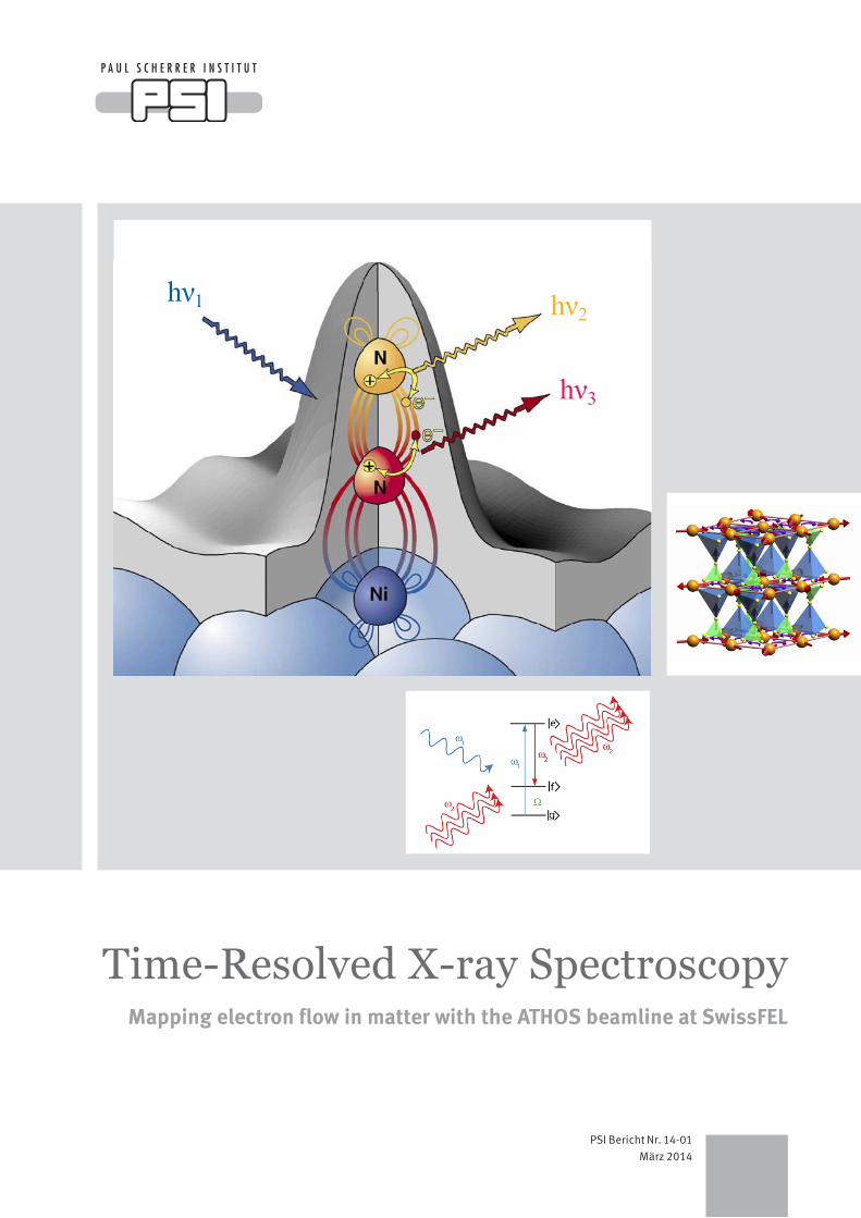
Left: Schematic representation of the “local probe” nature of soft X-ray spectroscopy, applied to an N2 molecule adsorbed on a nickel surface. The grey volume represents the electron density outside the metal surface, and the colored loops indicate a par-ticular molecular orbital, which extends over both nitrogen atoms and a surface nickel atom. Following excitation by an incoming energetic X-ray hν1, transitions between core and valence elec-tron states, indicated by arrows, produce fluorescence radiation at characteristic photon energies hν2 and hν3. These transitions are sensitive to the chemical binding of the two nitrogen atoms. The ATHOS beamline at SwissFEL will allow such site-specific probing of electronic binding to be performed in a time-resolved manner after driving the system out of chemical equilibrium, e.g., with an optical laser pulse. The figure is reproduced with the per-mission of the publisher from A. Nilsson and L.G.M. Pettersson, Surface Science Reports, 55, p. 49 (2004).
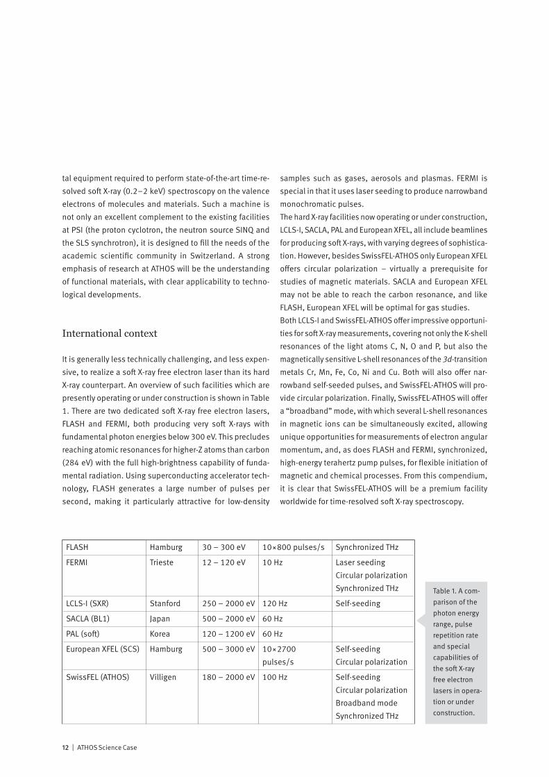
Right: The multiferroic state in RbFe(MoO4)2, as envisaged by M. Kenzelmann, PSI. Ordering of the magnetic moments (red arrows on the orange Fe atoms) leads to alternating spin currents on the
triangles (pink arrows), which, together with the alternating crys-tal field environment, generate a macroscopic ferroelectric polari-zation (transparent vertical blue arrows). Using the ATHOS beamline at SwissFEL, one may study the transient effect of an applied electric field on the magnetic order, with potential appli-cations in novel switching devices.
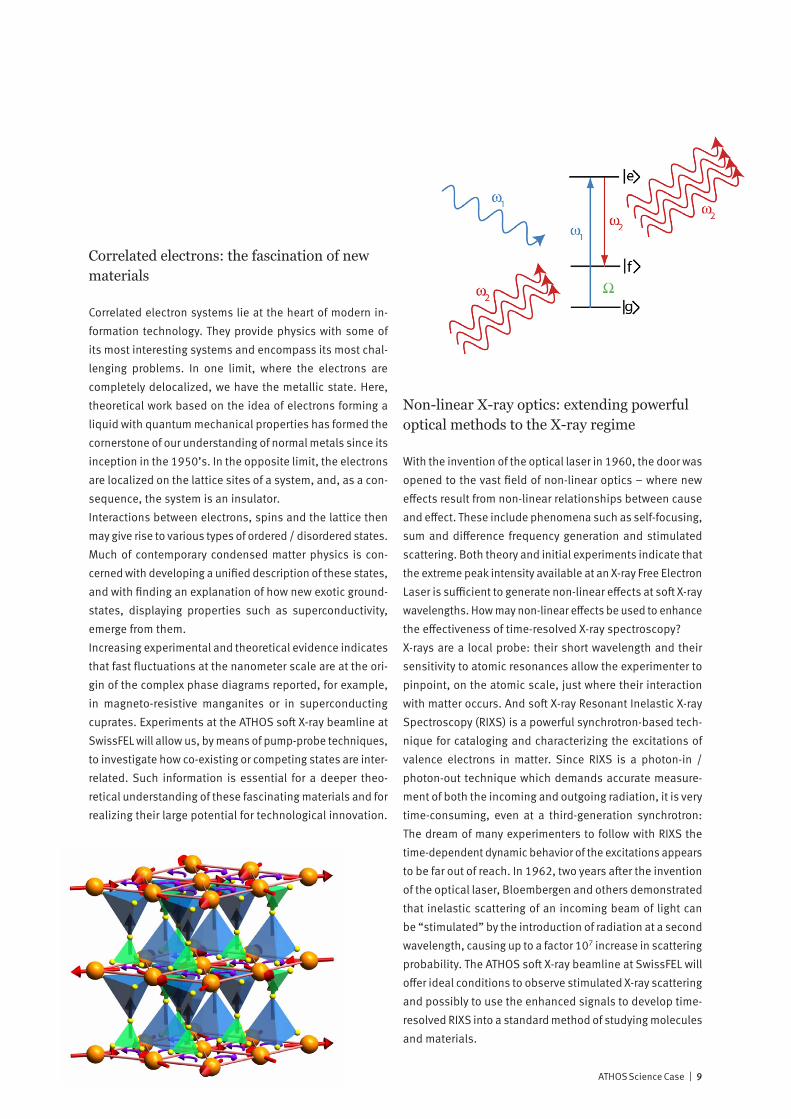
Lower: With sufficiently intense pulses of soft X-rays, it should be possible to observe phenomena beyond the linear regime, in an extension to X-ray wavelengths of the vast field of non-linear optics with visible lasers. The figure schematically shows a stim-ulated X-ray Raman scattering process, where intense pulses of resonant X-rays, at the two frequencies ω1 and ω2, are simultane-ously incident on a three-level atomic system. The result is the annihilation of the “pump” photon ω1 and the inelastic creation of a phase-coherent “Stokes” photon ω2, leaving the system in the excited state Ω. The ATHOS beamline at SwissFEL may make such processes much more probable than non-stimulated inelas-tic scattering, allowing time-resolved inelastic spectroscopy to be routinely performed.
Editorial Board
Bruce D. Patterson and Mirjam van Daalen
With contributions from:
Time-resolved surface chemistryM. Nielsen (Copenhagen)E. Aziz (BESSY)M. Wolf (FHI Berlin)N. Bukowiecki (EMPA)M. Ammann (PSI)M. Chergui (EPFL)J. van Bokhoven (ETHZ)T. Schmitt (PSI)J. Osterwalder (Uni Zh)
Ultrafast magnetism and correlated electron systemsR. Hertel (Jülich)H. Brune (EPFL)P. Gambardella (ETHZ)C. Back (Regensburg)M. Kenzelmann (PSI)H. Rønnow (EPFL)A. Vaterlaus (ETHZ)F. Mila (EPFL)P. Wernet (HZB, Berlin)M. Fiebig (ETHZ)U. Staub (PSI)Ch. Rüegg (PSI, Uni Geneva)H. Dil (Uni ZH, PSI)T. Schmitt (PSI)S. Johnson (ETHZ)P. van Loosdrecht (Köln)D. van der Marel (Uni GE)F. Nolting (PSI, Uni Basel)V. Strocov (PSI)R. Allenspach (IBM Lab, Rüschlikon)
Non-linear X-ray opticsG. Knopp (PSI)P. Abbamonte (Illinois, USA)W. Würth (Hamburg)D.C. Urbanek (South Carolina, USA)M. Chergui (EPFL)J. Nordgren (Uppsala)S. Mukamel (Irvine, USA)T. Feurer (Uni BE)
ATHOS Science Case | 3
Table of Contents
5 Foreword
6 ScientificChallenges
10 Introduction and ATHOS Project Overview
16 I. Ultrafast Magnetization Dynamics on the Nanoscale Temporal spin behavior in magnetic solids at short length scales
30 II. Following Catalysis and Biochemistry with Soft X-Rays Electronic transfer and redistribution in functional molecules
46 III. Time-Resolved Spectroscopy of Correlated Electron Materials Mapping the flow of energy among strongly-correlated degrees of freedom
66 IV. Non-Linear X-Ray Optics Can the field of non-linear optics be extended to the X-ray regime?
78 The XFEL Operating Principle
82 Appendix: ATHOS Workshops

4 | ATHOS Science Case
PSI condensed matter and biology research will be pursued with completely new experiments at the ATHOS beamline at SwissFEL.
ATHOS Science Case | 5
The principal mission of the Paul Scherrer Institute consists in developing, constructing and operating complex large-scale facilities for cutting-edge research, aimed at providing solutions to important scientific and technological chal-lenges facing modern society, in the fields of Matter and Materials, Energy and the Environment, and Human Health. The planned realization in 2017 of the ARAMIS X-ray beam-line at the SwissFEL free electron laser facility will establish PSI as a major center for ultrafast studies using hard X-rays. It will enable time-resolved structural studies of molecules and materials, to answer the question: “Where are the at-oms, and how do they move?”The properties and behavior of materials are to a large degree determined by the distribution and dynamics of their chem-ically and electronically most active electrons, the so-called valence electrons. Soft X-ray spectroscopy, as is performed, for example at the Swiss Light Source at PSI, is an ideal tool for studying arrangements of such valence electrons. But in order to visualize the electronic dynamics, for example in disordered catalysts or nano-scale quantum dots, time-re-solved spectroscopy is required.The design of the SwissFEL facility has foreseen the addition of the ATHOS beamline, including associated optics and experimental stations, to perform state-of-the-art time-re-
solved X-ray spectroscopy on functional materials. Such a development will be of great benefit to both academia and industry, within Switzerland and internationally. As the other facilities at PSI, it will be a focus for world-class researchers, education of young scientists and creation of high-technol-ogy jobs.The present document discusses unsolved scientific ques-tions and possible means for their solution using time-re-solved soft X-ray spectroscopic techniques. The compilation is the work of approximately 20 research groups, from Switzerland and abroad (see inside cover), together with the PSI staff. Some of the material has appeared in the original SwissFEL Science Case and has been reproduced here in an updated form.PSI welcomes the challenges involved in realizing the ATHOS beamline at SwissFEL and is proud to provide to the scientific community with an outstanding facility for time-resolved soft X-ray spectroscopy.
Joël MesotDirector, Paul Scherrer Institut
Time-Resolved X-ray spectroscopy: to meet challenges facing society
6 | ATHOS Science Case
ScientificChallenges
Of vital importance in today’s world are functional molecules and materials. These can be catalytic systems to produce plastics, purify gases or synthesize fuels, ultrafast electronic switches and high-capacity magnetic storage media in in-formation technology, or molecular complexes which govern cellular function and cause hereditary disease. The cogs in such functional molecules and materials are the valence electrons, which, due to their electric charge, light mass and moderate binding energy, determine the physical, chemical and biological properties of matter. For the same reasons, it is also the valence electrons which interact with external influences such as electromagnetic fields, optical excitation and neighboring reactive species. Since the advent of the optical laser in 1960, time-resolved optical spectroscopy has been developed into a powerful tool for investigating the properties of valence electrons in matter. A drawback of optical spectroscopy, however, is its general inability to determine the position on the atomic scale of the electrons being observed – information which is often only available from theoretical predictions.With soft X-ray spectroscopy, however, one can use well-defined resonant atomic transitions to specifically address particular electron orbitals. In this way, for example, one can determine the chemical valence of a metal ion in a biological complex, or the symmetry of d-electrons in a cuprate super-conductor, or the spin and orbital angular momenta of a particular ion in a magnetic material. For this reason, a vari-
ety of soft X-ray spectroscopies are now bread-and-butter techniques at the many synchrotrons in operation worldwide.In order to observe and quantify the functionality of matter in the time domain, it is necessary to follow the dynamics of valence electrons on their natural time scale. These time scales τ, in turn, are related by the Heisenberg uncertainty principle to the characteristic energy scales E involved, via the relation τ = h/E, where Planck’s constant h = 4.14 eVfs. Hence, the dynamics of a valence electron with a typical interaction energy 1 eV must be probed on the time scale of 4 femtoseconds. Synchrotron pulses generally have a duration longer than 50 picoseconds – a factor of 7000 too slow. Only at a soft X-ray Free Electron Laser, such as the ATHOS beamline at SwissFEL, does one have the combina-tion of peak intensity, wavelength tunability and fs pulse length required to perform dynamic soft X-ray spectroscopy in the time domain.The hard X-rays which will be available at the ARAMIS beam-line at SwissFEL will allow one to follow the motion of atoms (an atom moving at the speed of sound requires 1 ps to travel 1 nm). The ATHOS soft X-ray beamline will immensely extend the capabilities of SwissFEL to dynamic soft X-ray spectroscopy and hence to the detailed study of functional molecules and materials. Direct beneficiaries of this exten-sion will be the chemical, materials and biological develop-ment programs at PSI, but also at Swiss universities and in international academic and industrial research laboratories.

ATHOS Science Case | 7
Magnetism: materials and processes for tomorrow’s information technology
The pace of development of modern technology is astound-ing, mirroring society’s need for high-performance devices, such as computers and mobile phones. These devices in-volve ever-increasing complexity, smaller components and higher data-storage capacity, which in turn demands the technological advancement of magnetic systems and poses ever more fundamental questions involving magnetism at faster time scales and on smaller length scales. Such de-mands and questions fuel new possibilities for exceptional measurements with a soft X-ray free electron laser. Consider the example of current-induced magnetic domain-wall mo-tion: although predicted over thirty years ago, it is only through recent advances in measurement instrumentation, lithography systems and film deposition techniques that this important effect could be implemented, measured and understood.When it comes to developing a sound scientific basis for future applications of magnetism, we are faced with three major challenges. Firstly, we need to understand novel in-teractions within a magnetic system, such as spin-torque phenomena involving a spin current, and the manipulation of spin structures with femtosecond laser pulses. Secondly, modern technology needs to be faster, moving into the femtosecond regime in order to dramatically accelerate in-formation transfer. For this, it will be essential to understand and develop ultrafast magnetic processes. Finally, the de-velopment of new magnetic materials and the understand-ing of their behavior will be essential. This includes na-
noscale magnets, which will meet the need for smaller device components, and complex multicomponent systems with multifunctional properties.If we are to continue to develop new technologies based on magnetic materials, address the major challenges in mag-netism and create paradigm shifts in scientific development, it will be essential to understand the fundamental processes in magnetic systems. For this, the ATHOS soft X-ray beamline at SwissFEL will provide a powerful tool, with its combination of high spatial resolution, to reveal the details of the spin structures, high temporal resolution, to observe both repeat-able and stochastic magnetic events, and elemental speci-ficity, to observe these processes in the individual compo-nents of a complex magnetic system.
8 | ATHOS Science Case
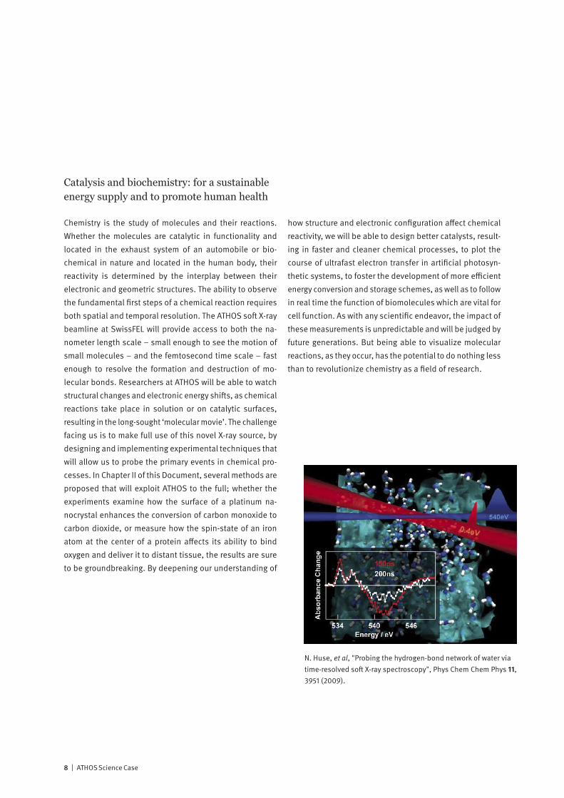
Catalysis and biochemistry: for a sustainable energy supply and to promote human health
Chemistry is the study of molecules and their reactions. Whether the molecules are catalytic in functionality and located in the exhaust system of an automobile or bio-chemical in nature and located in the human body, their reactivity is determined by the interplay between their electronic and geometric structures. The ability to observe the fundamental first steps of a chemical reaction requires both spatial and temporal resolution. The ATHOS soft X-ray beamline at SwissFEL will provide access to both the na-nometer length scale – small enough to see the motion of small molecules – and the femtosecond time scale – fast enough to resolve the formation and destruction of mo-lecular bonds. Researchers at ATHOS will be able to watch structural changes and electronic energy shifts, as chemical reactions take place in solution or on catalytic surfaces, resulting in the long-sought ‘molecular movie’. The challenge facing us is to make full use of this novel X-ray source, by designing and implementing experimental techniques that will allow us to probe the primary events in chemical pro-cesses. In Chapter II of this Document, several methods are proposed that will exploit ATHOS to the full; whether the experiments examine how the surface of a platinum na-nocrystal enhances the conversion of carbon monoxide to carbon dioxide, or measure how the spin-state of an iron atom at the center of a protein affects its ability to bind oxygen and deliver it to distant tissue, the results are sure to be groundbreaking. By deepening our understanding of
how structure and electronic configuration affect chemical reactivity, we will be able to design better catalysts, result-ing in faster and cleaner chemical processes, to plot the course of ultrafast electron transfer in artificial photosyn-thetic systems, to foster the development of more efficient energy conversion and storage schemes, as well as to follow in real time the function of biomolecules which are vital for cell function. As with any scientific endeavor, the impact of these measurements is unpredictable and will be judged by future generations. But being able to visualize molecular reactions, as they occur, has the potential to do nothing less than to revolutionize chemistry as a field of research.
N. Huse, et al, "Probing the hydrogen-bond network of water via time-resolved soft X-ray spectroscopy", Phys Chem Chem Phys 11, 3951 (2009).
ATHOS Science Case | 9
Correlated electrons: the fascination of new materials
Correlated electron systems lie at the heart of modern in-formation technology. They provide physics with some of its most interesting systems and encompass its most chal-lenging problems. In one limit, where the electrons are completely delocalized, we have the metallic state. Here, theoretical work based on the idea of electrons forming a liquid with quantum mechanical properties has formed the cornerstone of our understanding of normal metals since its inception in the 1950’s. In the opposite limit, the electrons are localized on the lattice sites of a system, and, as a con-sequence, the system is an insulator. Interactions between electrons, spins and the lattice then may give rise to various types of ordered / disordered states. Much of contemporary condensed matter physics is con-cerned with developing a unified description of these states, and with finding an explanation of how new exotic ground-states, displaying properties such as superconductivity, emerge from them. Increasing experimental and theoretical evidence indicates that fast fluctuations at the nanometer scale are at the ori-gin of the complex phase diagrams reported, for example, in magneto-resistive manganites or in superconducting cuprates. Experiments at the ATHOS soft X-ray beamline at SwissFEL will allow us, by means of pump-probe techniques, to investigate how co-existing or competing states are inter-related. Such information is essential for a deeper theo-retical understanding of these fascinating materials and for realizing their large potential for technological innovation.
Non-linear X-ray optics: extending powerful optical methods to the X-ray regime
With the invention of the optical laser in 1960, the door was opened to the vast field of non-linear optics – where new effects result from non-linear relationships between cause and effect. These include phenomena such as self-focusing, sum and difference frequency generation and stimulated scattering. Both theory and initial experiments indicate that the extreme peak intensity available at an X-ray Free Electron Laser is sufficient to generate non-linear effects at soft X-ray wavelengths. How may non-linear effects be used to enhance the effectiveness of time-resolved X-ray spectroscopy?X-rays are a local probe: their short wavelength and their sensitivity to atomic resonances allow the experimenter to pinpoint, on the atomic scale, just where their interaction with matter occurs. And soft X-ray Resonant Inelastic X-ray Spectroscopy (RIXS) is a powerful synchrotron-based tech-nique for cataloging and characterizing the excitations of valence electrons in matter. Since RIXS is a photon-in / photon-out technique which demands accurate measure-ment of both the incoming and outgoing radiation, it is very time-consuming, even at a third-generation synchrotron: The dream of many experimenters to follow with RIXS the time-dependent dynamic behavior of the excitations appears to be far out of reach. In 1962, two years after the invention of the optical laser, Bloembergen and others demonstrated that inelastic scattering of an incoming beam of light can be “stimulated” by the introduction of radiation at a second wavelength, causing up to a factor 107 increase in scattering probability. The ATHOS soft X-ray beamline at SwissFEL will offer ideal conditions to observe stimulated X-ray scattering and possibly to use the enhanced signals to develop time-resolved RIXS into a standard method of studying molecules and materials.

10 | ATHOS Science Case
Introduction and Project OverviewThe ATHOS beamline at SwissFEL – a national facility for time-resolved soft X-ray spectroscopy
Organization of the ATHOS Science Case
The present document, the Science Case for the ATHOS beamline at SwissFEL, is organized as follows:
• An introduction defines the mission, strategy and design considerations of the facility and places the project in the national and international research arenas. An overview is given of the project time-schedule.
• The scientific case for the ATHOS beamline at SwissFEL, in the research areas of magnetism, catalysis and biochemistry, correlated electron materials and non-linear X-ray optics, is then
presented in four chapters, written at approximately the level of a graduate student in natural science. A number of blue “Infoboxes” have been included to provide additional background information.
• The operating principle of an X-ray free electron laser, including some mathematical physics, is then presented.
• The appendix lists the scientific workshops which have formed the basis of this scientific case, and the research groups which have contributed are listed on the inside cover.

ATHOS Science Case | 11
ScientificMotivation
The ATHOS beamline will extend the capabilities of the SwissFEL X-ray laser to include time-resolved soft X-ray spectroscopy, providing a powerful tool for the study of the dynamics of valence electrons in matter (see Fig. 1). It is the weakly-bound valence electrons which determine the phys-ical, chemical and biological characteristics of molecules and materials and their interactions with external influences. With tunable soft X-ray photons, in the energy range of 0.2–2 keV, the experimenter has the unique possibility of probing such electrons, e.g., their energetics and spatial distribution and symmetry, in an elemental and chemically specific manner. If, as will be the case at ATHOS, the photons have a variable polarization, the electronic spin and orbital angular momenta in magnetic materials can in addition be determined. Static measurements of this type represent a major field of activity at the many synchrotron facilities worldwide. Intense, short-duration soft X-ray pulses from an X-ray free electron laser allow for the first time dynamic spectroscopic measurements to be performed on the natu-ral time scale of the valence electrons – femtoseconds to
picoseconds. With such a tool, one can begin to answer such questions as: “How rapidly can the magnetization of a sample be reversed?” “What path is taken by a photo-excited electron in a catalyst from generation to reaction?” “How do strong correlations among valence electrons cause the appearance of new quantum phases in matter?” Answers to these and related questions are sorely needed, both for technological development in Switzerland and to understand and protect our world.
Realization
The SwissFEL X-ray laser facility at PSI is a marvel of innova-tive high-technology, precise engineering and scientific curiosity. Beginning in 2017, the first beamline, ARAMIS, will deliver intense, ultrafast pulses of hard X-rays (2–14 keV) to experiments, which will follow the motion of atoms in matter. In the SwissFEL design, provision has been made to accommodate an additional X-ray beamline. The ATHOS project at SwissFEL will outfit this beamline with the electron accelerator, magnet undulator, X-ray optics and experimen-
Fig. 1. The spectrum of photon ener-gies and wavelengths provided by SwissFEL, in the hard X-ray regime by ARAMIS and in the soft X-ray regime by ATHOS. The red, blue and green cir-cles mark selected K, L and M-edge atomic resonances. In the “water window”, there is a high contrast for imaging biological material (which is absorbing) in water (which is trans-parent). Magnetism and correlated electron phenomena are particularly accessible with soft X-ray spectros-copy at the L-edges of the 3d transi-tion-metal ions (600–1000 eV). ATHOS will also cover the resonances of many adsorbates and substrates in important catalytic systems.
12 | ATHOS Science Case
tal equipment required to perform state-of-the-art time-re-solved soft X-ray (0.2–2 keV) spectroscopy on the valence electrons of molecules and materials. Such a machine is not only an excellent complement to the existing facilities at PSI (the proton cyclotron, the neutron source SINQ and the SLS synchrotron), it is designed to fill the needs of the academic scientific community in Switzerland. A strong emphasis of research at ATHOS will be the understanding of functional materials, with clear applicability to techno-logical developments.
International context
It is generally less technically challenging, and less expen-sive, to realize a soft X-ray free electron laser than its hard X-ray counterpart. An overview of such facilities which are presently operating or under construction is shown in Table 1. There are two dedicated soft X-ray free electron lasers, FLASH and FERMI, both producing very soft X-rays with fundamental photon energies below 300 eV. This precludes reaching atomic resonances for higher-Z atoms than carbon (284 eV) with the full high-brightness capability of funda-mental radiation. Using superconducting accelerator tech-nology, FLASH generates a large number of pulses per second, making it particularly attractive for low-density
samples such as gases, aerosols and plasmas. FERMI is special in that it uses laser seeding to produce narrowband monochromatic pulses.The hard X-ray facilities now operating or under construction, LCLS-I, SACLA, PAL and European XFEL, all include beamlines for producing soft X-rays, with varying degrees of sophistica-tion. However, besides SwissFEL-ATHOS only European XFEL offers circular polarization – virtually a prerequisite for studies of magnetic materials. SACLA and European XFEL may not be able to reach the carbon resonance, and like FLASH, European XFEL will be optimal for gas studies.Both LCLS-I and SwissFEL-ATHOS offer impressive opportuni-ties for soft X-ray measurements, covering not only the K-shell resonances of the light atoms C, N, O and P, but also the magnetically sensitive L-shell resonances of the 3d-transition metals Cr, Mn, Fe, Co, Ni and Cu. Both will also offer nar-rowband self-seeded pulses, and SwissFEL-ATHOS will pro-vide circular polarization. Finally, SwissFEL-ATHOS will offer a “broadband” mode, with which several L-shell resonances in magnetic ions can be simultaneously excited, allowing unique opportunities for measurements of electron angular momentum, and, as does FLASH and FERMI, synchronized, high-energy terahertz pump pulses, for flexible initiation of magnetic and chemical processes. From this compendium, it is clear that SwissFEL-ATHOS will be a premium facility worldwide for time-resolved soft X-ray spectroscopy.
FLASH Hamburg 30 – 300 eV 10×800 pulses/s Synchronized THz
FERMI Trieste 12 – 120 eV 10 Hz Laser seeding Circular polarization Synchronized THz
LCLS-I (SXR) Stanford 250 – 2000 eV 120 Hz Self-seeding
SACLA (BL1) Japan 500 – 2000 eV 60 Hz
PAL (soft) Korea 120 – 1200 eV 60 Hz
European XFEL (SCS) Hamburg 500 – 3000 eV 10×2700 pulses/s
Self-seeding Circular polarization
SwissFEL (ATHOS) Villigen 180 – 2000 eV 100 Hz Self-seeding Circular polarization Broadband mode Synchronized THz
Table 1. A com-parison of the photon energy range, pulse repetition rate and special capabilities of the soft X-ray free electron lasers in opera-tion or under construction.

ATHOS Science Case | 13
Design of ATHOS at SwissFEL
The ATHOS soft X-ray beamline at SwissFEL (Fig. 2) will com-plement the hard X-ray beamline ARAMIS, which will go into operation in 2017. The building and accelerator construction presently underway makes provision for ATHOS, including the beam divider after LINAC 2 and space for the tuning LI-NAC, the ATHOS undulator, the soft X-ray optics and the ATHOS experimental stations. The last of these will be flex-ibly located situated in a single large hall.ATHOS will have several special features, to enhance the quality of the X-ray pulses delivered to the experiments. In order to allow the simultaneous operation of ARAMIS and ATHOS, a “two bunch mode” of SwissFEL operation is being developed, in which, with its 100 Hz repetition rate, Swiss-FEL will accelerate two electron bunches, separated by 28 ns. The first of these will be further accelerated by LINAC 3 to produce hard X-rays in the ARAMIS undulator, and the second will be deflected to the tuning LINAC, to undergo a final energy adjustment, and on to the ATHOS undulator, to produce soft X-rays. Thus, experiments at both ARAMIS and ATHOS can be simultaneously served with X-ray pulses at a repetition rate of 100 Hz.Another feature of ATHOS is the ability, using variable heli city undulators of the APPLE II type, to produce soft X-rays with variable polarization. With this feature, the user can specify a linear polarization, either horizontal or vertical, or right or left circular polarization. As described in Chapter I, this capability is particularly important for investigations of
dynamic magnetism. The use of a helical undulator, as op-posed to a local polarization rotation using a short “polar-izing afterburner” undulator section, will produce an excep-tionally high degree of polarization.As discussed in Chapter IV, the SASE (self-amplified spon-taneous emission) pulses emitted by a generic XFEL have a poor longitudinal coherence: both the time and spectral profiles of the X-ray pulses show pronounced spikes, and the relative spectral bandwidth is typically 0.3%. The band-width can be reduced at the experimental station by the use of a monochromater, but this will increase shot-to-shot in-tensity variations in the pulse intensity and, for hard X-rays, will lengthen the pulse duration. A much more elegant al-ternative for improving longitudinal coherence is to “seed” the XFEL pulse amplification by introducing into the undula-tor light pulses at a well-defined frequency equal to or at a sub-harmonic of the XFEL emission frequency. As the seed pulse propagates with the emitting electrons, only the seeded frequency component undergoes strong amplifica-tion, and a narrow-band, nearly Gaussian, output pulse results, with a relative bandwidth of only 0.001%. At Swiss-FEL, an optional seeding mode of operation is planned for both ARAMIS and ATHOS using the concept of “self-seeding” [1]. In this scheme, a monochromating optical filter sur-rounded by an electron bypass chicane is introduced at approximately the half-way point along the XFEL undulator (see Fig. 3). Spontaneously emitted light from an electron bunch in the first undulator half is filtered by the monochro-mator and, after assuring both spatial and temporal overap,
Fig. 2. A schematic overview of the SwissFEL facility, showing the ARAMIS hard X-ray beamline, scheduled for operation in 2017, and the ATHOS soft X-ray beamline.

14 | ATHOS Science Case
is injected together with the delayed electron bunch into the second undulator half. Here the filtered seed pulse is efficiently amplified, to produce a narrow-band output pulse.At ARAMIS, the hard X-rays will be seeded using a diamond crystal filter [2], and at ATHOS, seeding will be realized by a compact arrangement of mirrors and gratings [3]. A simu-lation of the resulting reduction in spectral bandwidth for ATHOS is shown in Fig. 3.Instead of narrowband pulses, some experiments at both ARAMIS and ATHOS will benefit from very broadband pulses. This is particularly true for spectroscopic measurements, where as much information as possible is to be extracted from a single XFEL pulse – the spectral information is then obtained from a dispersive detection arrangement. In the soft X-ray range, sufficiently broadband single-shot spec-troscopy will allow the simultaneous observation of both
the L2 and L3 absorption edges in magnetic 3d transition-metal ions, allowing the separate determination of the spin and orbital angular momentum of the ion. The method used, X-ray magnetic circular dichoroism (XMCD) is described in detail in Chapter I. SwissFEL, due to the use of compact, high-frequency (C-band) acceleration modules, will have the ability, if desired, to “overchirp” the electron bunches, thus producing exceptionally broadband X-ray pulses, with a relative bandwidth of from 3 to 7% [4]. As shown in Fig. 4, this will be sufficient to cover the L2 and L3 edges.In time-resolved “pump-probe” experiments, the initiating pump pulse, often from an optical laser, is just as important as the probe pulse, i.e., the soft X-ray pulse from ATHOS. Like ARAMIS, the ATHOS facility will provide a wide range of short-duration, high-intensity, optically-generated pump pulses, from the infrared to the ultraviolet. As described in
Fig. 5. Because of the 28 ns delay between the ARAMIS and ATHOS electron bunches, sufficient time is available to transport coherent synchrotron radiation (CSR) from the spent ARAMIS bunches to use as THz pump pulses at the ATHOS experiments.
Fig. 4. Measured XMCD spectra for a cobalt film, with right and left circularly-polarized soft X-rays. Simultaneous absorption measurements at the L2 and L3 resonances, as will be possible with the SwissFEL broadband mode, will allow single-shot determination of both spin and orbital an-gular moments. See Chapter I for details.
Fig. 3. Left: Schematic arrangement for soft X-ray self-seeding. Blue = electrons, red = X-rays.Right: Simulated spectra for a SASE (red) and a self-seeded (blue) pulse at the ATHOS beamline at SwissFEL [5]. Different vertical scales are used for the two cases: In reality, the spectral brightness of the seeded pulse exceeds that of the SASE pulse by approximately a factor 40.
ATHOS Science Case | 15
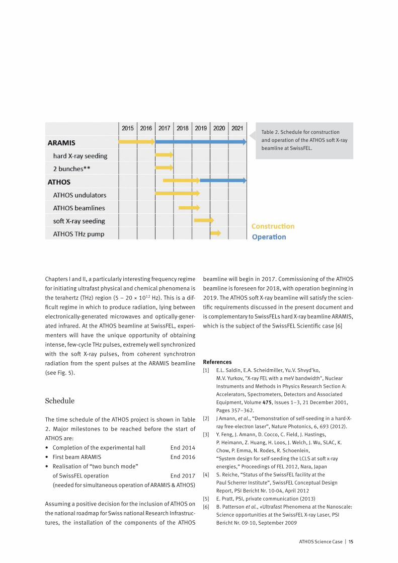
Chapters I and II, a particularly interesting frequency regime for initiating ultrafast physical and chemical phenomena is the terahertz (THz) region (5 – 20 × 1012 Hz). This is a dif-ficult regime in which to produce radiation, lying between electronically-generated microwaves and optically-gener-ated infrared. At the ATHOS beamline at SwissFEL, experi-menters will have the unique opportunity of obtaining intense, few-cycle THz pulses, extremely well synchronized with the soft X-ray pulses, from coherent synchrotron radiation from the spent pulses at the ARAMIS beamline (see Fig. 5).
Schedule
The time schedule of the ATHOS project is shown in Table 2. Major milestones to be reached before the start of ATHOS are:• Completion of the experimental hall End 2014• First beam ARAMIS End 2016• Realisation of “two bunch mode” of SwissFEL operation End 2017 (needed for simultaneous operation of ARAMIS & ATHOS)
Assuming a positive decision for the inclusion of ATHOS on the national roadmap for Swiss national Research Infrastruc-tures, the installation of the components of the ATHOS
beamline will begin in 2017. Commissioning of the ATHOS beamline is foreseen for 2018, with operation beginning in 2019. The ATHOS soft X-ray beamline will satisfy the scien-tific requirements discussed in the present document and is complementary to SwissFELs hard X-ray beamline ARAMIS, which is the subject of the SwissFEL Scientific case [6]
References[1] E.L. Saldin, E.A. Scheidmiller, Yu.V. Shvyd’ko,
M.V. Yurkov, "X-ray FEL with a meV bandwidth", Nuclear Instruments and Methods in Physics Research Section A: Accelerators, Spectrometers, Detectors and Associated Equipment, Volume 475, Issues 1–3, 21 December 2001, Pages 357–362.
[2] J Amann, et al., “Demonstration of self-seeding in a hard-X-ray free-electron laser”, Nature Photonics, 6, 693 (2012).
[3] Y. Feng, J. Amann, D. Cocco, C. Field, J. Hastings, P. Heimann, Z. Huang, H. Loos, J. Welch, J. Wu, SLAC, K. Chow, P. Emma, N. Rodes, R. Schoenlein, “System design for self-seeding the LCLS at soft x-ray energies,” Proceedings of FEL 2012, Nara, Japan
[4] S. Reiche, “Status of the SwissFEL facility at the Paul Scherrer Institute”, SwissFEL Conceptual Design Report, PSI Bericht Nr. 10-04, April 2012
[5] E. Pratt, PSI, private communication (2013)[6] B. Patterson et al., «Ultrafast Phenomena at the Nanoscale:
Science opportunities at the SwissFEL X-ray Laser, PSI Bericht Nr. 09-10, September 2009
Table 2. Schedule for construction and operation of the ATHOS soft X-ray beamline at SwissFEL.

16 | ATHOS Science Case
Magnetism is responsible for one of the oldest inventions, the magnetic compass, and further applications have revolutionized our world, through, e.g., ferrite core memory to today’s high-density data storage. In modern magnetic storage devices, of the order of 700 gigabits can be written per square inch at a rate of one bit per two nanoseconds. Faster reversal, on the sub-ps time scale, has been demonstrated, but its origins still remain to be investigated.
The fact that many fundamental magnetic processes take place on the nanom-eter length and picosecond time scales, and the high magnetic sensitivity of resonant, circularly-polarized X-rays, make the ATHOS beamline at SwissFEL a versatile instrument for state-of-the-art research in magnetism. Of particular current interest are the ultrafast disappearance, creation and modification of magnetic order. The SwissFEL, with coherent, high-brightness, circularly-polarized X-rays at energies resonant with the 3d-transition metal ions, corresponding to nm wavelengths, is capable of single-shot lensless imaging of nanometer-scale magnetic structures. Furthermore, the combination of high-energy, half-cycle THz pump pulses and the synchronized, sub-picosecond SwissFEL probe pulses will permit the investigation in real time of ultrafast magnetic interactions.
I. Ultrafast Magnetization Dynamics on the NanoscaleTemporal spin behavior in magnetic systems at short length and time scales
• Time and length scales in magnetism
• Magnetically sensitive X-ray measurement techniques
• Ultrafast manipulation of the magnetization
ATHOS Science Case | 17
Table 1.2: Magnetic time scales.
Table I.1: Magnetic length scales.
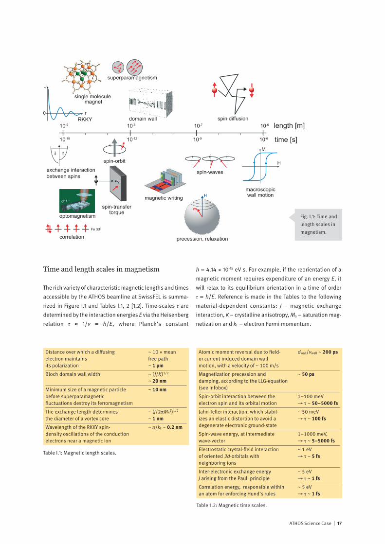
Fig. I.1: Time and length scales in magnetism.
Time and length scales in magnetism
The rich variety of characteristic magnetic lengths and times accessible by the ATHOS beamline at SwissFEL is summa-rized in Figure I.1 and Tables I.1, 2 [1,2]. Time-scales τ are determined by the interaction energies E via the Heisenberg relation τ ≈ 1/ν = h/E, where Planck’s constant
h = 4.14 × 10⁻¹⁵ eV s. For example, if the reorientation of a magnetic moment requires expenditure of an energy E, it will relax to its equilibrium orientation in a time of order τ = h/E. Reference is made in the Tables to the following material-dependent constants: J – magnetic exchange interaction, K – crystalline anisotropy, Ms – saturation mag-netization and kF – electron Fermi momentum.
Atomic moment reversal due to field- dwall/vwall ~ 200 ps or current-induced domain wall motion, with a velocity of ~ 100 m/s Magnetization precession and ~ 50 ps damping, according to the LLG-equation (see Infobox) Spin-orbit interaction between the 1–100 meV electron spin and its orbital motion → τ ~ 50–5000 fsJahn-Teller interaction, which stabil- ~ 50 meV izes an elastic distortion to avoid a → τ ~ 100 fs degenerate electronic ground-state Spin-wave energy, at intermediate 1–1000 meV, wave-vector → τ ~ 5–5000 fsElectrostatic crystal-field interaction ~ 1 eV of oriented 3d-orbitals with → τ ~ 5 fs neighboring ions Inter-electronic exchange energy ~ 5 eV J arising from the Pauli principle → τ ~ 1 fsCorrelation energy, responsible within ~ 5 eV an atom for enforcing Hund’s rules → τ ~ 1 fs
Distance over which a diffusing ~ 10 × mean electron maintains free path its polarization ~ 1 μm Bloch domain wall width ~ (J/K)1/2 ~ 20 nmMinimum size of a magnetic particle ~ 10 nm before superparamagnetic fluctuations destroy its ferromagnetismThe exchange length determines ~ (J/2πMs2)1/2 the diameter of a vortex core ~ 1 nmWavelength of the RKKY spin- ~ π/kF ~ 0.2 nm density oscillations of the conduction electrons near a magnetic ion
10-15
10-9 10-8 10-7
spin diffusion
10-12 10-9
10-6
10-6 time [s]
length [m]
0RKKY
single molecule magnet
J
r
spin-orbit
exchange interaction between spins
correlation
optomagnetism
spin-waves
macroscopicwall motion
precession, relaxation
M
H
superparamagnetism
m
H
Fe 3d6
spin-transfertorque
domain wall
magnetic writing
18 | ATHOS Science Case
Magnetically sensitive X-ray measurement techniques
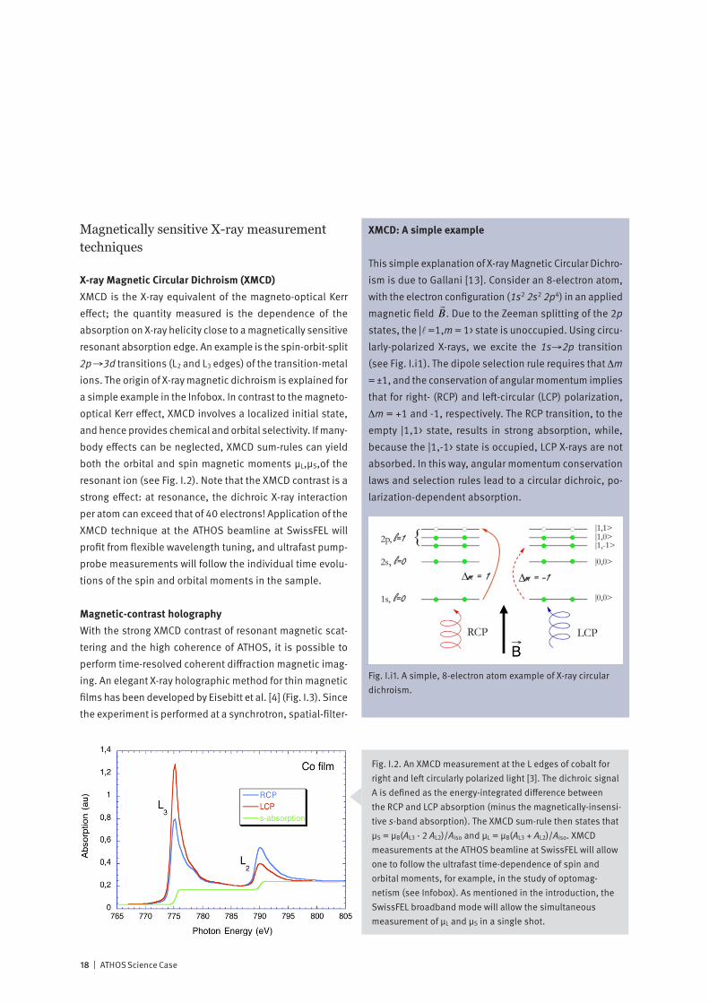
X-ray Magnetic Circular Dichroism (XMCD)XMCD is the X-ray equivalent of the magneto-optical Kerr effect; the quantity measured is the dependence of the absorption on X-ray helicity close to a magnetically sensitive resonant absorption edge. An example is the spin-orbit-split 2p→3d transitions (L2 and L3 edges) of the transition-metal ions. The origin of X-ray magnetic dichroism is explained for a simple example in the Infobox. In contrast to the magneto-optical Kerr effect, XMCD involves a localized initial state, and hence provides chemical and orbital selectivity. If many-body effects can be neglected, XMCD sum-rules can yield both the orbital and spin magnetic moments μL,μS,of the resonant ion (see Fig. I.2). Note that the XMCD contrast is a strong effect: at resonance, the dichroic X-ray interaction per atom can exceed that of 40 electrons! Application of the XMCD technique at the ATHOS beamline at SwissFEL will profit from flexible wavelength tuning, and ultrafast pump-probe measurements will follow the individual time evolu-tions of the spin and orbital moments in the sample.
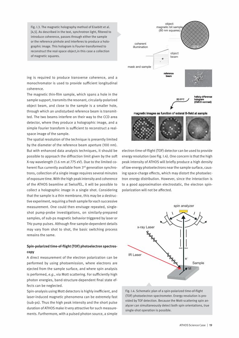
Magnetic-contrast holographyWith the strong XMCD contrast of resonant magnetic scat-tering and the high coherence of ATHOS, it is possible to perform time-resolved coherent diffraction magnetic imag-ing. An elegant X-ray holographic method for thin magnetic films has been developed by Eisebitt et al. [4] (Fig. I.3). Since the experiment is performed at a synchrotron, spatial-filter-
Fig. I.2. An XMCD measurement at the L edges of cobalt for right and left circularly polarized light [3]. The dichroic signal A is defined as the energy-integrated difference between the RCP and LCP absorption (minus the magnetically-insensi-tive s-band absorption). The XMCD sum-rule then states that μS = μB(AL3 - 2 AL2)/Aiso and μL = μB(AL3 + AL2)/Aiso. XMCD measurements at the ATHOS beamline at SwissFEL will allow one to follow the ultrafast time-dependence of spin and orbital moments, for example, in the study of optomag-netism (see Infobox). As mentioned in the introduction, the SwissFEL broadband mode will allow the simultaneous measurement of μL and μS in a single shot.
XMCD: A simple example
This simple explanation of X-ray Magnetic Circular Dichro-ism is due to Gallani [13]. Consider an 8-electron atom, with the electron configuration (1s2 2s2 2p4) in an applied magnetic field
€
B . Due to the Zeeman splitting of the 2p states, the |l =1,m = 1> state is unoccupied. Using circu-larly-polarized X-rays, we excite the 1s→2p transition (see Fig. I.i1). The dipole selection rule requires that Δm = ±1, and the conservation of angular momentum implies that for right- (RCP) and left-circular (LCP) polarization, Δm = +1 and -1, respectively. The RCP transition, to the empty |1,1> state, results in strong absorption, while, because the |1,-1> state is occupied, LCP X-rays are not absorbed. In this way, angular momentum conservation laws and selection rules lead to a circular dichroic, po-larization-dependent absorption.
Fig. I.i1. A simple, 8-electron atom example of X-ray circular dichroism.
→
ATHOS Science Case | 19
ing is required to produce transverse coherence, and a monochromator is used to provide sufficient longitudinal coherence.The magnetic thin-film sample, which spans a hole in the sample support, transmits the resonant, circularly-polarized object beam, and close to the sample is a smaller hole, through which an undisturbed reference beam is transmit-ted. The two beams interfere on their way to the CCD area detector, where they produce a holographic image, and a simple Fourier transform is sufficient to reconstruct a real-space image of the sample.The spatial resolution of the technique is presently limited by the diameter of the reference beam aperture (100 nm). But with enhanced data analysis techniques, it should be possible to approach the diffraction limit given by the soft X-ray wavelength (1.6 nm at 775 eV). Due to the limited co-herent flux currently available from 3rd generation synchro-trons, collection of a single image requires several minutes of exposure time. With the high peak intensity and coherence of the ATHOS beamline at SwissFEL, it will be possible to collect a holographic image in a single shot. Considering that the sample is a thin membrane, this may be a destruc-tive experiment, requiring a fresh sample for each successive measurement. One could then envisage repeated, single-shot pump-probe investigations, on similarly-prepared samples, of sub-ps magnetic behavior triggered by laser or THz pump pulses. Although fine sample-dependent details may vary from shot to shot, the basic switching process remains the same.
Spin-polarized time-of-flight (TOF) photoelectron spectros-copyA direct measurement of the electron polarization can be performed by using photoemission, where electrons are ejected from the sample surface, and where spin analysis is performed, e.g., via Mott scattering. For sufficiently high photon energies, band-structure-dependent final state ef-fects can be neglected. Spin-analysis using Mott detectors is highly inefficient, and laser-induced magnetic phenomena can be extremely fast (sub-ps). Thus the high peak intensity and the short pulse duration of ATHOS make it very attractive for such measure-ments. Furthermore, with a pulsed photon source, a simple
electron time-of-flight (TOF) detector can be used to provide energy resolution (see Fig. I.4). One concern is that the high peak intensity of ATHOS will briefly produce a high density of low-energy photoelectrons near the sample surface, caus-ing space-charge effects, which may distort the photoelec-tron energy distribution. However, since the interaction is to a good approximation electrostatic, the electron spin-polarization will not be affected.
MSample
spin analyzer
e–IR Laser
x-ray Laser
Fig. I.3. The magnetic holography method of Eisebitt et al. [4,5]. As described in the text, synchrotron light, filtered to introduce coherence, passes through either the sample or the reference pinhole and interferes to produce a holo-graphic image. This hologram is Fourier-transformed to reconstruct the real-space object,in this case a collection of magnetic squares.
Fig. I.4. Schematic plan of a spin-polarized time-of-flight (TOF) photoelectron spectrometer. Energy resolution is pro-vided by TOF detection. Because the Mott-scattering spin an-alyzer can simultaneously detect both spin orientations, true single-shot operation is possible.
CCD
object:magnetic bit sample
(80 nm squares)
coherentillumination
mask and sample
SEM
referencebeam
helicity differencehologram(XMCD contrast)
magnetic images as function of exteral B-field at sample
objectbeam
2D FFT
S. Eisebitt, private communication
objectbeam
20 | ATHOS Science Case
Ultrafast manipulation of the magnetization
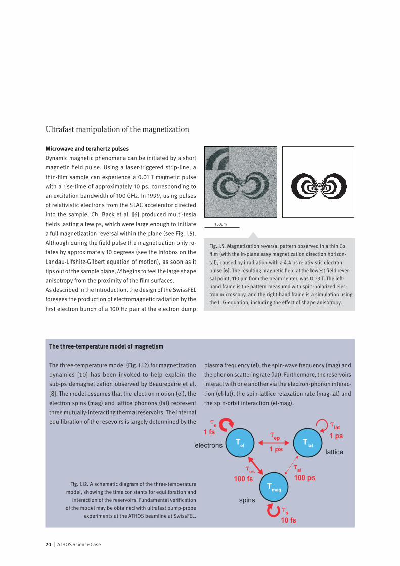
Microwave and terahertz pulsesDynamic magnetic phenomena can be initiated by a short magnetic field pulse. Using a laser-triggered strip-line, a thin-film sample can experience a 0.01 T magnetic pulse with a rise-time of approximately 10 ps, corresponding to an excitation bandwidth of 100 GHz. In 1999, using pulses of relativistic electrons from the SLAC accelerator directed into the sample, Ch. Back et al. [6] produced multi-tesla fields lasting a few ps, which were large enough to initiate a full magnetization reversal within the plane (see Fig. I.5). Although during the field pulse the magnetization only ro-tates by approximately 10 degrees (see the Infobox on the Landau-Lifshitz-Gilbert equation of motion), as soon as it tips out of the sample plane, M begins to feel the large shape anisotropy from the proximity of the film surfaces.As described in the Introduction, the design of the SwissFEL foresees the production of electromagnetic radiation by the first electron bunch of a 100 Hz pair at the electron dump
The three-temperature model of magnetism
The three-temperature model (Fig. I.i2) for magnetization dynamics [10] has been invoked to help explain the sub-ps demagnetization observed by Beaurepaire et al. [8]. The model assumes that the electron motion (el), the electron spins (mag) and lattice phonons (lat) represent three mutually-interacting thermal reservoirs. The internal equilibration of the resevoirs is largely determined by the
plasma frequency (el), the spin-wave frequency (mag) and the phonon scattering rate (lat). Furthermore, the reservoirs interact with one another via the electron-phonon interac-tion (el-lat), the spin-lattice relaxation rate (mag-lat) and the spin-orbit interaction (el-mag).
150µm
Fig. I.5. Magnetization reversal pattern observed in a thin Co film (with the in-plane easy magnetization direction horizon-tal), caused by irradiation with a 4.4 ps relativistic electron pulse [6]. The resulting magnetic field at the lowest field rever-sal point, 110 μm from the beam center, was 0.23 T. The left-hand frame is the pattern measured with spin-polarized elec-tron microscopy, and the right-hand frame is a simulation using the LLG-equation, including the effect of shape anisotropy.
Tel Tlat
�lat�e
1 fs
1 ps
1 ps
lattice
spins
electrons
100 ps100 fs
10 fs�s
�sl
�ep
�es
TmagFig. I.i2. A schematic diagram of the three-temperature
model, showing the time constants for equilibration and interaction of the reservoirs. Fundamental verification
of the model may be obtained with ultrafast pump-probe experiments at the ATHOS beamline at SwissFEL.

ATHOS Science Case | 21
of the ARAMIS beamline and the transport of this pulse to experiments at ATHOS, resulting in synchronized, high-energy, half-cycle pump pulses at terahertz frequencies (5-20 × 1012 Hz), which are synchronized with the X-ray probe pulses from ATHOS. The intensity (power/area) delivered by an electromagnetic pulse is I = B2
0 c/2µ0, implying that a 100 μJ, half-cycle THz pulse (0.5 ps) focused to 1 mm2 will produce a peak magnetic field B0 = 1.3 T, i.e., more than 100 times that of a strip-line, and with a THz excitation band-width. This offers the possibility of probing the ultimate limit of magnetization dynamics, which is at least a factor 1000 faster than conventional field-induced spin switching.A further possibility for rapidly perturbing the magnetic moments in a dynamic XMCD experiment is X-ray detected ferromagnetic resonance, using continuous-wave or pulsed microwave (GHz) radiation [7]. When resonant with the Zeeman-split energy levels of the magnetic ions, the micro-waves excite damped magnetic precession, the details of which are sensitive to dynamic couplings and magnetization relaxation. If several magnetic species are simultaneously present in the sample, the elemental selectivity of XMCD allows the dynamics of each to be studied individually. The high peak brightness and excellent time resolution of the SwissFEL would be very beneficial for this technique, avoid-ing the present restriction to samples with very low damping.
Laser-induced phenomenaIn 1996, Beaurepaire et al. published a very remarkable observation [8]: a Ni film exposed to an intense 60 fs pulse from an optical laser becomes demagnetized in less than a picosecond. Using the magneto-optical Kerr effect as probe, an ultrafast decrease is observed in the magnetization, fol-lowed by a slower recovery (see Fig. I.6). This observation, together with later measurements using other methods of detection, raised the fundamental question, as yet unan-swered, of where the spin angular momentum of the elec-trons goes and how it can be transferred so quickly.The three-temperature model, which invokes separate temperatures to characterize the electron kinetic energy (Tel), the electronic spin order (Tmag) and the lattice vibrations (Tlat) (see Infobox), has been used to describe the demag-netization process. It is assumed that the laser pump pulse initially delivers energy to the electron reservoir Tel and that
each reservoir individually remains in equilibrium. But due to their relatively weak intercoupling, the three temperatures may differ significantly at short time scales, giving rise to strong non-equilibrium effects which have not yet been investigated.Microscopic models have difficulty in explaining how the laser excitation of the conduction electrons can cause such a rapid transfer of angular momentum away from the spin system or indeed what is its destination. Among the propos-als put forward are: hiding the angular momentum in elec-tronic orbits, or transferring it to the lattice via special hot-spots in the electron band structure with exceptional spin-orbit coupling or via an enhancement of the spin-orbit interaction by the presence of phonons [9].A phenomenological treatment of the entire de- and remag-netization process using an atomic analog of the Landau-Lifshitz-Gilbert (LLG) equations (see Infobox), with the
Fig. I.6. Sub-picosecond demagnetization of a Ni film follow-ing an optical laser pulse, observed with the magneto-optical Kerr effect [8]. This observation stimulated much speculation on the as yet unanswered question of how angular momen-tum can be transferred so efficiently from the spin system to the lattice.

22 | ATHOS Science Case
Spin-torque: ultrafast switching by spin currents
Beyond the conventional switching by applied external fields, magnetization manipulation can also be achieved by using spin transfer from spin-polarized currents that flow in a magnetic structure. This leads to ultra-fast rever-sal of nano-pillar elements as well as current-induced domain wall motion. Here the magnetization dynamic timescales are not limited by the gyromagnetic ratio and can be potentially much faster.
Including a spin-polarized current (u→ is proportional to the current density and the spin-polarization of the current), the extended Landau-Lifschitz-Gilbert equation now reads:
!
" = #gLandeµB /h
!
d
r M
dt= "µ
0
r M #
r H +
$
Ms
r M #
d
r M
dt%
r u &
r ' ( )
r M
Ms
+ (
r M
Ms
#r u &
r ' ( )
r M
Ms
)
* +
,
- .
with the last two terms accounting for the adiabatic and non-adiabatic spin-torque. The strength of the effect is given by u and the non-adiabaticity parameter β.Spin currents can be generated by spin-injection, spin pumping and, on a femtosecond timescale, by exciting spin-polarized charge carriers with a fs laser [14]. Further-more, heating the electron system with a short laser pulse will generate large temperature gradients, and the result-ing spin currents and spin-torque-induced ultra-fast mag-netization dynamics can be ideally probed using the SwissFEL.
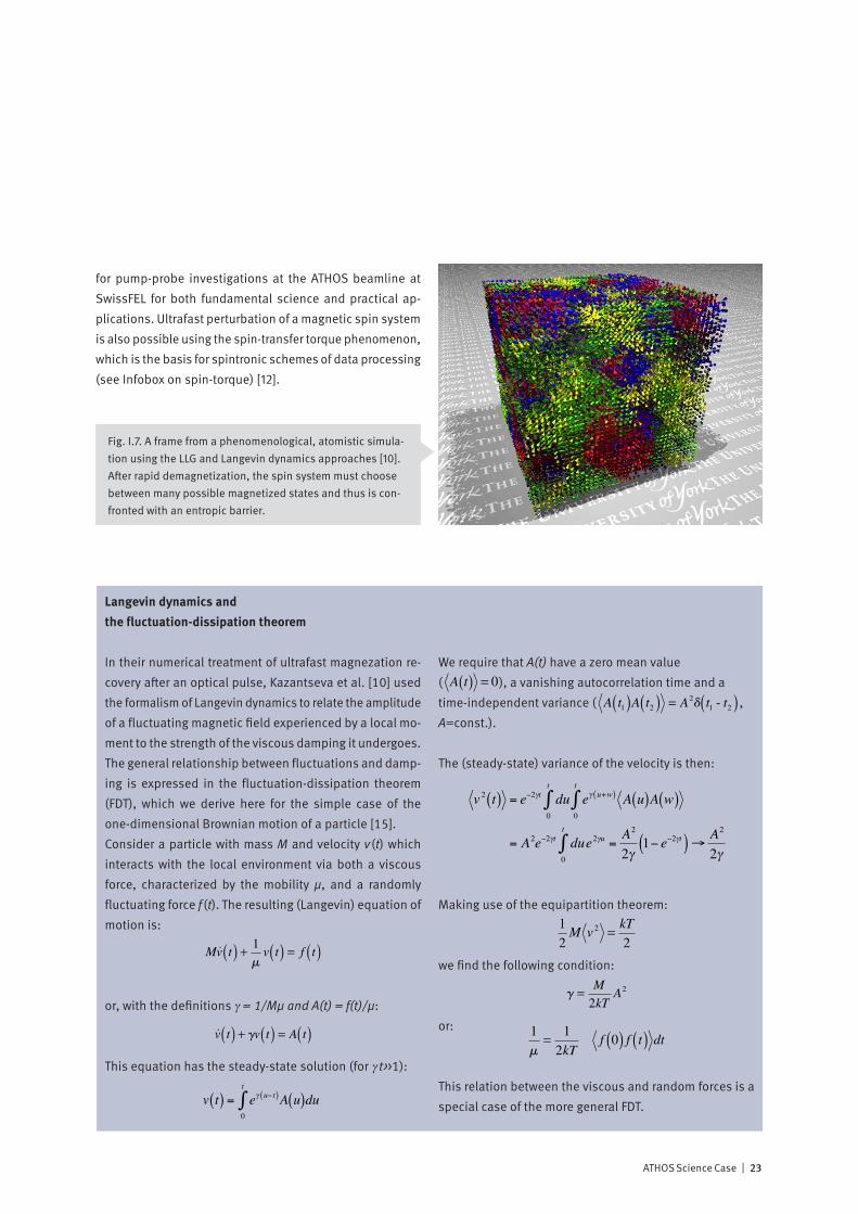
magnetization M replaced by the atomic spin S, has been published by Kazantseva et al. [10]. These authors intro-duced an effective field acting on the atomic moments, which includes a stochastic, fluctuating component, which they then related to the LLG damping constant α using the fluctuation-dissipation theorem (see Infobox).From their atomistic numerical simulations (see Fig. I.7), Kazantseva et al. [10] find that the magnetization can be non-zero in spite of a spin temperature Tmag which exceeds the Curie temperature of Ni (TC = 631 K), leading them to question the concept of equilibration of the spin system and hence of a spin temperature. The authors find that the coupling constant which governs the post-pulse recovery of the magnetization is the same as that responsible for the ultrafast demagnetization. They explain the much slower recovery, and the fact that the recovery is slower for a more complete demagnetization, with the concept of a magnetic entropic barrier (see also Chapter II) – i.e., if the magnetiza-tion vanishes, it takes time for the system to reorganize it-
self. In addition to this, now classic, example of ultrafast demagnetization, some systems show the phenomena of ultrafast magnetization. For example, intermetallic FeRh undergoes a transition at 360 K from a low-temperature anti-ferromagnetic phase to a high-temperature ferromag-netic phase, which is accompanied by an isotropic lattice expansion. This transition can be induced by an ultrashort laser pulse [11]. Preliminary results using 50 ps X-ray probe pulses from a synchrotron suggest that the establishment of ferromagnetic order precedes the increase in lattice constant, possibly answering the chicken-or-egg question as to which is the cause and which is the effect. Finally, in experiments with a direct connection to magnetic data storage, it has been found that ultrafast pulses of cir-cularly-polarized laser light can, perhaps via the inverse Faraday effect, even reverse the direction of magnetization in a sample (see the optomagnetism Infobox). The above examples of the ultrafast manipulation of magnetization with optical pulses point to a rich variety of possibilities
ATHOS Science Case | 23
Langevin dynamics and the fluctuation-dissipation theorem
In their numerical treatment of ultrafast magnezation re-covery after an optical pulse, Kazantseva et al. [10] used the formalism of Langevin dynamics to relate the amplitude of a fluctuating magnetic field experienced by a local mo-ment to the strength of the viscous damping it undergoes. The general relationship between fluctuations and damp-ing is expressed in the fluctuation-dissipation theorem (FDT), which we derive here for the simple case of the one-dimensional Brownian motion of a particle [15]. Consider a particle with mass M and velocity v (t) which interacts with the local environment via both a viscous force, characterized by the mobility μ, and a randomly fluctuating force f (t). The resulting (Langevin) equation of motion is:
�
M ˙ v t( ) + 1
mv t( ) = f t( )
or, with the definitions γ = 1/Mμ and A(t) = f(t)/μ:
�
˙ v t( ) + gv t( ) = A t( )
This equation has the steady-state solution (for γ t>>1):
!
v t( ) = e" u# t( )
0
t
$ A u( )du
!
v2t( ) = e"2#t du
0
t
$ e# u+w( )
0
t
$ A u( )A w( )
= A2e"2#t
du
0
t
$ e2#u =
A2
2#1" e"2#t( )%
A2
2#
We require that A(t) have a zero mean value (
�
A t( ) = 0 ), a vanishing autocorrelation time and a time-independent variance (
�
A t1( )A t2( ) = A2d t1 - t2( ) , A=const.).
The (steady-state) variance of the velocity is then:
!
v t( ) = e" u# t( )
0
t
$ A u( )du
!
v2t( ) = e"2#t du
0
t
$ e# u+w( )
0
t
$ A u( )A w( )
= A2e"2#t
du
0
t
$ e2#u =
A2
2#1" e"2#t( )%
A2
2#
Making use of the equipartition theorem:
�
1
2M v 2 = kT
2
we find the following condition:
�
g = M
2kTA2
or:
�
1
m= 1
2kTf 0( ) f t( ) dt
This relation between the viscous and random forces is a special case of the more general FDT.
Fig. I.7. A frame from a phenomenological, atomistic simula-tion using the LLG and Langevin dynamics approaches [10]. After rapid demagnetization, the spin system must choose between many possible magnetized states and thus is con-fronted with an entropic barrier.
for pump-probe investigations at the ATHOS beamline at SwissFEL for both fundamental science and practical ap-plications. Ultrafast perturbation of a magnetic spin system is also possible using the spin-transfer torque phenomenon, which is the basis for spintronic schemes of data processing (see Infobox on spin-torque) [12].
24 | ATHOS Science Case
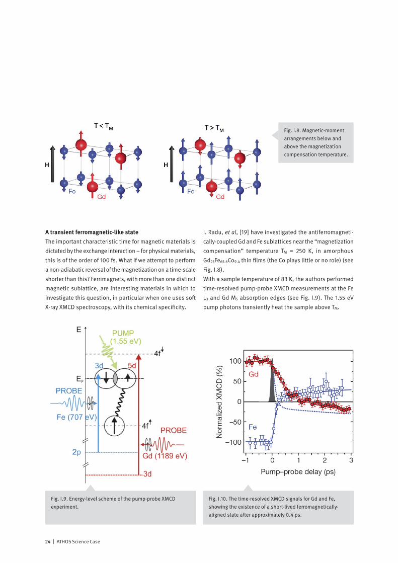
A transient ferromagnetic-like stateThe important characteristic time for magnetic materials is dictated by the exchange interaction – for physical materials, this is of the order of 100 fs. What if we attempt to perform a non-adiabatic reversal of the magnetization on a time-scale shorter than this? Ferrimagnets, with more than one distinct magnetic sublattice, are interesting materials in which to investigate this question, in particular when one uses soft X-ray XMCD spectroscopy, with its chemical specificity.
I. Radu, et al, [19] have investigated the antiferromagneti-cally-coupled Gd and Fe sublattices near the “magnetization compensation” temperature TM = 250 K, in amorphous Gd25Fe65.6Co9.4 thin films (the Co plays little or no role) (see Fig. I.8).With a sample temperature of 83 K, the authors performed time-resolved pump-probe XMCD measurements at the Fe L3 and Gd M5 absorption edges (see Fig. I.9). The 1.55 eV pump photons transiently heat the sample above TM.
Fig. I.8. Magnetic-moment arrangements below and above the magnetization compensation temperature.
Fig. I.9. Energy-level scheme of the pump-probe XMCD experiment.
Fig. I.10. The time-resolved XMCD signals for Gd and Fe, showing the existence of a short-lived ferromagnetically-aligned state after approximately 0.4 ps.
ATHOS Science Case | 25
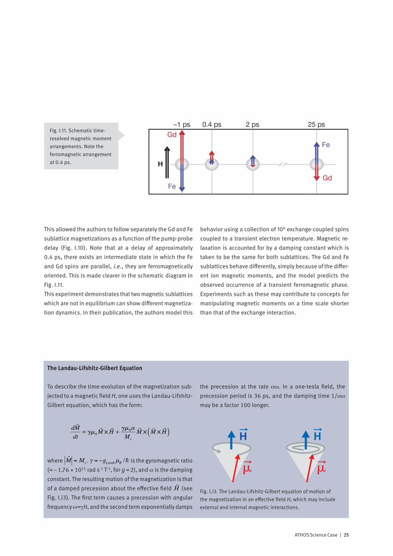
This allowed the authors to follow separately the Gd and Fe sublattice magnetizations as a function of the pump-probe delay (Fig. I.10). Note that at a delay of approximately 0.4 ps, there exists an intermediate state in which the Fe and Gd spins are parallel, i.e., they are ferromagnetically oriented. This is made clearer in the schematic diagram in Fig. I.11.This experiment demonstrates that two magnetic sublattices which are not in equilibrium can show different magnetiza-tion dynamics. In their publication, the authors model this
behavior using a collection of 106 exchange-coupled spins coupled to a transient electron temperature. Magnetic re-laxation is accounted for by a damping constant which is taken to be the same for both sublattices. The Gd and Fe sublattices behave differently, simply because of the differ-ent ion magnetic moments, and the model predicts the observed occurrence of a transient ferromagnetic phase. Experiments such as these may contribute to concepts for manipulating magnetic moments on a time scale shorter than that of the exchange interaction.
Fig. I.11. Schematic time- resolved magnetic moment arrangements. Note the ferromagnetic arrangement at 0.4 ps.
The Landau-Lifshitz-Gilbert Equation
To describe the time-evolution of the magnetization sub-jected to a magnetic field H, one uses the Landau-Lifshitz-Gilbert equation, which has the form:
�
d
M
dt= gm0
M x
H + gm0a
Ms
M x
M x
H ( )
where
!
r M = Ms. " = #gLandeµB /h is the gyromagnetic ratio
(= –1.76 × 10¹¹ rad s-1 T-1, for g =2), and α is the damping constant. The resulting motion of the magnetization is that of a damped precession about the effective field
€
H (see Fig. I.i3). The first term causes a precession with angular frequency ω=γH, and the second term exponentially damps
the precession at the rate αω. In a one-tesla field, the precession period is 36 ps, and the damping time 1/αω may be a factor 100 longer.
�
H
precession
�
H
dampingFig. I.i3. The Landau-Lifshitz-Gilbert equation of motion of the magnetization in an effective field H, which may include external and internal magnetic interactions.
26 | ATHOS Science Case
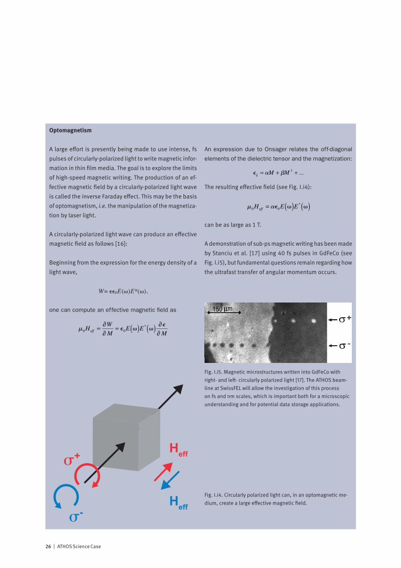
Optomagnetism
A large effort is presently being made to use intense, fs pulses of circularly-polarized light to write magnetic infor-mation in thin film media. The goal is to explore the limits of high-speed magnetic writing. The production of an ef-fective magnetic field by a circularly-polarized light wave is called the inverse Faraday effect. This may be the basis of optomagnetism, i.e. the manipulation of the magnetiza-tion by laser light.
A circularly-polarized light wave can produce an effective magnetic field as follows [16]:
Beginning from the expression for the energy density of a light wave,
W= 0E()E*(),
one can compute an effective magnetic field as
�
m0Heff = ∂W
∂M= e0E v( )E * v( ) ∂e
∂M
An expression due to Onsager relates the off-diagonal
elements of the dielectric tensor and the magnetization:
�
eij = aM + bM 3 + ...
The resulting effective field (see Fig. I.i4):
�
m0Heff = ae0E v( )E * v( )
can be as large as 1 T. A demonstration of sub-ps magnetic writing has been made by Stanciu et al. [17] using 40 fs pulses in GdFeCo (see Fig. I.i5), but fundamental questions remain regarding how the ultrafast transfer of angular momentum occurs.
Fig. I.i5. Magnetic microstructures written into GdFeCo with right- and left- circularly polarized light [17]. The ATHOS beam-line at SwissFEL will allow the investigation of this process on fs and nm scales, which is important both for a microscopic understanding and for potential data storage applications.
Heff
Heff
�+
�-
Fig. I.i4. Circularly polarized light can, in an optomagnetic me-dium, create a large effective magnetic field.

ATHOS Science Case | 27
Magnetic vortex core switching
The magnetic vortex is a very stable, naturally-forming magnetic configuration occurring in thin soft-magnetic nanostructures. Due to shape anisotropy, the magnetic moments in such thin-film elements lie in the film plane. The vortex configuration is characterized by the circulation of the in-plane magnetic structure around a very stable core of only a few tens of nanometers in diameter, of the order of the exchange length. A particular feature of this structure is the core of the vortex, which is perpendicu-larly magnetized relative to the sample plane. This results in two states: “up” or “down”. Their small size and perfect stability make vortex cores promising candidates for mag-netic data storage.A study by Hertel et al. [18] based on micromagnetic simulations (LLG equation) has shown that, strikingly, the
core can dynamically be switched between “up” and “down” within only a few tens of picoseconds by means of an external field. Figure I.i6 simulates the vortex core switching in a 20 nm thick Permalloy disk of 200 nm di-ameter after the application of a 60 ps field pulse, with a peak value of 80 mT. Using field pulses as short as 5 ps, the authors show that the core reversal unfolds first through the production of a new vortex with an oppositely oriented core, followed by the annihilation of the original vortex with a transient antivortex structure.To date, no experimental method can achieve the required temporal (a few tens of ps) and spatial (a few tens of nm) resolution to investigate this switching process. The com-bination of the high-energy THz pump source and circular-ly-polarized ATHOS probe pulses will allow such studies.
60 nm
30
0 10 20ps
40 50
Fig. I.i6. Numerical simulation [18] of the proposed switching process of a magnetic vortex core. The ATHOS beamline at SwissFEL will provide the spatial and temporal resolution rquired to visualize this process.

28 | ATHOS Science Case
Summary
• Present magnetic storage devices are limited to densities of 700 gigabits/square inch (i.e. one bit/1000 nm2) and reading/writing times of 2 ns, while standard synchrotron-based magnetic studies are limited by the 100 ps pulse duration. The ATHOS beamline at SwissFEL will investigate magnetic phenomena well beyond these values.
• Fundamental magnetic interactions occur on the nanometer and sub-picosecond length and time scales – which are very well matched to the capabilities of the ATHOS beamline at SwissFEL.
• With its provision of circularly-polarized radiation, high transverse coherence and femtosecond pulse duration, the ATHOS beamline at SwissFEL will accommodate the X-ray measurement techniques of particular relevance to ultrafast magnetism: X-ray magnetic circular dichroism (XMCD), magnetic-contrast holography and time-of-flight, spin-analyzed photoemission.
• A synchronized terahertz pump source at the ATHOS beamline at SwissFEL will provide magnetic field pulses with an amplitude of approximately 1 Tesla and a duration of approximately 1 picosecond, for high-bandwidth excitation in ultrafast pump-probe experiments.
• Synchronized femtosecond pulses of optical laser light will also be available for pumping at the ATHOS beamline at SwissFEL. These cause rapid heating of the electrons of the sample, which, through as yet not understood interactions, may demagnetize a sample, cause a transition from an antiferromagnetic to a ferromagnetic state, reverse the magnetization direction or create unusual transient states. Pump-probe XMCD experiments at the ATHOS beamline at SwissFEL will follow the ultrafast behavior of the spin and orbital moments during these processes.
• With the broadband operation mode of SwissFEL, it will be possible, using XMCD, to simultaneously determine both the spin and orbital moments of a magnetic ion.
ATHOS Science Case | 29
References
[1] Vaz, C. A. F., Bland, J. A. C., and Lauhoff, G., “Magnetism in ultrathin film structures,” Rep. Prog. Phys. 71, 056501 (2008).
[2] Stöhr, J. and Siegmann, H. C., Magnetism: From Fundamentals to Nanoscale Dynamics (Springer, Berlin, 2006).
[3] Courtesy of A. Fraile Rodriguez.[4] Eisebitt, S., et al., “Lensless imaging of magnetic
nanostructures by X-ray spectro-holography,” Nature 432, 885-888 (2004).
[5] Eisebitt, S., (private communication).[6] Back, C. H., et al., “Minimum field strength in
precessional magnetization reversal,” Science 285, 864-867 (1999).
[7] Boero, G., et al., “Double-resonant X-ray and microwave absorption: Atomic spectroscopy of precessional orbital and spin dynamics,” Phys. Rev. B 79, 224425 (2008).
[8] Beaurepaire, E., Merle, J. C., Daunois, A., and Bigot, J. Y., “Ultrafast spin dynamics in ferromagnetic nickel,” Phys. Rev. Lett. 76, 4250-4253 (1996).
[9] Koopmans, B., Kicken, H., Van Kampen, M., and de Jonge, W. J. M., “Microscopic model for femtosecond magnetization dynamics,” J. Magn. Magn. Mater. 286, 271-275 (2005).
[10] Kazantseva, N., Nowak, U., Chantrell, R. W., Hohlfeld, J., and Rebei, A., “Slow recovery of the magnetisation after a sub-picosecond heat pulse,” Europhys. Lett. 81, 27004 (2008).
[11] Thiele, J. U., Buess, M., and Back, C. H., “Spin dynamics of the antiferromagnetic-to-ferromagnetic phase transition in FeRh on a sub-picosecond time scale,” Appl. Phys. Lett. 85, 2857-2859 (2004).
[12] Prinz, G.A., “Device physics-magnetoelectronics“, Science 282, 1660-1663 (1998).
[13] Gallani, J.-L., private communication.[14] Malinowski, G., Longa, F.D., Rietjens, J.H.H., Paluskar, P.V.,
Huijink, R. Swagten, H.J.M. & Koopmans, B., “Control of speed and efficiency of ultrafast demagnetization by direct transfer of spin angular momentum“, Nature Physics 4, 855-858 (2008).
[15] Cowan, B. Topics in Statistical Mechanics (World Scientific, Singapore, 2005).
[16] Ziel, J. P. v. d., P.S.Pershan, and L.D.Malstrom, “Opti cally-induced magnetization resulting from the inverse Faraday effect,” Phys. Rev. Lett. 15, 190-193 (1965).
[17] Stanciu, C. D., et al., “All-optical magnetic recording with circularly polarized light,” Phys. Rev. Lett. 99, 047601 (2007).
[18] Hertel, R., Gliga, S., Fahnle, M., and Schneider, C.M., “Ultrafast nanomagnetic toggle switching of vortex cores,” Phys. Rev. Lett. 98, 117201 (2007).
[19] Radu, I., et al, “Transient ferromagnetic-like state meditating ultrafast reversal of antiferromagnetically coupled spins”, Nature 472, 205 (2011).
30 | ATHOS Science Case
Valence electrons, distributed in bonding and anti-bonding molecular orbitals, determine the chemical properties of inorganic and organic matter. Their dy namics, on the sub-picosecond time scale, are responsible for the atomic rearrangements we call chemistry. The elemental and even chemical specificity of soft X-ray spectroscopy, performed at the K-absorption edges of the light ele-ments C, O and N and the L-absorption edges of the 3d transition metal elements Ti, Mn, Fe, and Cu provide a powerful tool to probe the valence electron distribu-tions, and when combined with the femtosecond time resolution of the SwissFEL, allow real-time studies of photo-triggered chemical reactions.
II. Following catalysis and biochemistry with soft X-raysDetermining how electron-transfer leads to molecular rearrangements – for the well-being of the planet and for its inhabitants
• Time and length scales in catalysis and biochemistry
• Photochemistry
• X-ray spectroscopic probes for chemistry
• Pump-probe investigations of chemical and biochemical dynamics

ATHOS Science Case | 31
Time and length scales in catalysis and biochemistry
Ultrafast processes in solution chemistryA principal application of the ATHOS beamline at SwissFEL will be the study of molecular dynamics and reactivity in catalytic systems, both in solution and on surfaces. Time scales of a range of chemical phenomena in solution are shown in Figure II.1. At the slow end of the scale is the dif-fusional rotation of a molecule in a solvent. The recombina-tion of photo-dissociated molecules occurs on the ps to ns scales, depending upon whether the recombining reactants arise from the same (geminate) or different (non-geminate) parent molecules. Several types of deactivation processes may occur in an intact photoexcited molecule: “Internal conversion” (10–100 fs) is an electronic reconfiguration in which the total electronic spin is conserved, while slower “intersystem crossing” (1–10 ns) involves a change of spin. Molecular cooling and vibrational energy transfer from a high to a low vibrational state generally occur in 1–100 ps. The exchange of a water molecule in the solvation shell
surrounding an ion requires approximately 250 ps, and further ultrafast processes in ionized water are shown sche-matically in Figure II.2, including the formation and stabili-zation of the solvated electron within 1 ps, which has proven to be critically important in both photocatalysis and elec-trochemistry [1].
Fundamental events in heterogeneous catalysisCatalysis is the enabling technology in a large number of processes for the production of goods, the provision of clean energy, and for pollution abatement. Heterogeneous ca-talysis occurs at the interface between a gas or liquid and a solid catalytic surface; the surface of a catalytically active solid provides an energy landscape which enhances reactiv-ity. A large number of processes are active here on the na-nometer scale, with characteristic times ranging from sub-fs, for electron transfer, to minutes, for the oscillating patterns studied by Ertl et al. [2] and to even months, for the deacti-vation of catalytic processes. The cartoon in Figure II.3 “schematically depicts, at the molecular level, the richness of the phenomena involved in the transformation of reactants
10-15
internalconversion
solvationdynamics
non-geminaterecombination
diffusionalrotation
S = 0c = c
10-12 10-9 10-6
time [s]
S = 0
intersystemcrossing
vibrationalcooling
dissociation andgeminate
recombination
S = 1S = 0
vibration
Fig. II.1: The time scales for chemical processes in solution match well the capabilities of the ATHOS beamline at SwissFEL.

32 | ATHOS Science Case
to products at the surface of a material. A molecule may scatter off the surface, experiencing no or some finite degree of energy exchange with the surface. Alternatively, molecule-surface energy transfer can lead to accommodation and physical adsorption or chemical adsorption. In some cases, physisorption is a precursor to chemisorption, and in some cases, bond dissociation is required for chemisorption. Charge transfer plays a critical role in some adsorption processes. Once on the surface, the adsorbed intermediates
may diffuse laterally with a temperature-dependent rate, sampling surface features including adatoms, vacancies and steps. They may become tightly bound to a defect site. Various adsorbed intermediates may meet, either at defect sites or at regular lattice sites, and form short-lived transition state structures and ultimately product molecules. Finally, products desorb from the surface with a temperature de-pendent rate, imparting some fraction of the energy of the association reaction to the surface” [3].
IonizingRadiation Ground state
electron attachment
dissociationrecombination
deexcitationOH H2
hν
O-H-
Preexisting trap?
Solvation
SolvatedElectron
10-1000 fsHydration
<300 fs
<100 fs
~0 fsExcitation
~1 ps
~? fsProton Transfer
*
*
-
Gas PhaseProducts
ScatteringDesorption
AssociativeDesorption
Diffusion DissociativeAdsorption
ChargeTransfer
Accomodation
PhysicalAdsorption
Gas PhaseReactants
AdsorbedIntermediates
TransitionStates
AdsorbedReactants
Adatom
Vacancy
Step Edge
Molecule-SurfaceEnergy
Transfer
Fig. II.2. Ultrafast processes in water, following a photoioni-zation event [1]. The formation and stabilization of a solvated electron (lower right) is fundamental in photocatalysis and radiation chemistry.
Fig. II.3. A schematic representation of the wide range of ultrafast nanoscale phenomena occuring on a catalytic surface [3].

ATHOS Science Case | 33
Wavepacket dynamicsWithin the Born-Oppenheimer approximation, as a chemical system moves from a configuration of high energy towards a potential minimum, the electrons are assumed to instan-taneously follow the motion of the much heavier nuclei. The uncertainty in nuclear position during the reaction is then represented by a wavepacket, and the time development during the reaction can be viewed as the motion of the packet along a trajectory on the potential energy surface. A sche-matic impulsive photo-excitation process and the resulting wavepacket motion are shown in Figure II.4, where one sees that for a typical 0.1 nm atomic displacement and 100 fs vibrational timescale, the velocity for wave-packet motion is of order 1000 m/s. It should be noted that the Born-Op-penheimer approximation may break down, particularly for light chemical elements. Such non-adiabatic couplings are prevalent at critical points on the potential energy surface, where two surfaces repel one another at an avoided crossing, or where they meet at a point – a conical intersection. It is at these critical points that chemical reactions occur. Also at metal surfaces, non-adiabatic couplings are frequently observed between adsorbate motion and electronic excita-tions in the metal substrate.
Time and length scales of biochemical reactionsThe biological length scales pertinent to SwissFEL applica-tions span the spectrum from individual atomic bonds and small molecules, such as glucose, in the subnanometer range, over individual protein molecules (e.g., hemoglobin) and molecular complexes (e.g., ribosomes) in the 1–10 nm range, over virus particles and cell organelles (10–100 nm), to entire cells (1 μm) (see Fig. II.5). With the hard X-radiation (λ ≈ 0.1 nm) available from the ARAMIS beamline at SwissFEL, single-shot coherent diffraction imaging of biological nano-structures is feasible at approximately 20 nm resolution [4]. With soft X-ray spectroscopy at the ATHOS beamline at SwissFEL, time-resolved changes in functional biomolecules can be followed on a wide range of time scales. The vibration period of the two carbon atoms in the ethene molecule against their mutual double bond is 20 fs, and such mo-lecular vibrations also set the time scale for photo-dissoci-ation processes, for example for the photo-detachment of CO from a heme group (i.e., an iron atom surrounded by a porphyrin ring). As biomolecular units increase in size, from methyl groups (0.3 nm) to side-chains (1 nm) to loops (4 nm) to large protein domains (8 nm), collective motions with long periods populate the crowded vibrational density of states. Although electron transfer processes can in principle be very fast, their speed is generally limited by that of mo-lecular reconformation. The same is true for decaging pro-cesses – the activation of a biomolecule by the photo-re-moval of a deactivating cage group.
Fig. II.5. The time and length scales for biochemical processes. Time-resolved soft X-ray spectroscopy at the ATHOS beamline at SwissFEL will access ultrafast changes in biomolecules.
Fig. II.4. Impulsive photo-excitation of a molecule in the wave-packet picture. During a typical reaction, the excited-state packet moves a distance of the order of ΔR = 1 Å.

34 | ATHOS Science Case
Photochemistry
Photo-initiation of catalysisSince important chemical processes are often irreversible, principal applications of the ATHOS beamline at SwissFEL will employ the pump-probe method: An external fast trigger, e.g., an optical, IR, or THz pulse, initiates a reaction, typically involving vibration, relaxation, and/or dissociation, and ATHOS delivers a synchronized soft-X-ray pulse to probe the subsequent processes. Historically, ultrafast chemistry experiments have been performed with fs laser pump pulses as the reaction initiator. The intriguing possibility of using non-ionizing THz radiation to initiate a surface catalytic reaction in the electronic ground state is the subject of an Infobox. As with the majority of high-intensity SwissFEL experiments, it will be necessary to refresh the sample between measurements, for example using a high-speed liquid jet for solutions (see Infobox) or a movable surface for catalytic reactions. In a solution environment, optical
pump pulses pose a problem in the ultrafast regime: As the desired time resolution improves, not only the probe pulse, but also the pump pulse must become shorter. Since it is the pump energy which determines the degree of photoex-citation in the sample, the peak intensity must increase as the pulse duration decreases. When a large number of photons are delivered in such a short period of time, com-peting excitation processes in both the sample and the solvent become increasingly relevant. In order to avoid such potential complications as nonlinear sample excitation, multiphoton solvent ionization and, at longer pump wave-lenths, tunneling ionization, a balance must be maintained between generating a sufficient level of sample excitation and ensuring that only the photoreaction of interest is being probed, and not a highly excited plasma. To achieve this balance, it will be necessary to perform laser spectroscopic pump-probe measurements in the optical regime prior to the SwissFEL measurements, using the same pump condi-tions as will be used with the X-ray probe.
THz initiation of surface reactions
The intensity (power/area) delivered by an electro-mag-netic wave is
�
I = e0E02c / 2 , implying that a half-cycle 100
μJ pulse of THz radiation, focused to 1 mm2, will produce a peak electric field E0 = 4 × 10⁸ V/m, which is comparable to the field exerted on an adsorbed atom by a scanning tunneling microscope tip used to manipulate atoms [15]. One thus envisages the collective control of atomic posi-tions using the THz pulse (Fig. II.i1).Since the phonon frequencies of the host and the local vibration frequencies of adsorbed atoms and molecules lie in the terahertz region, THz pulses can resonantly excite these modes. Finally, E0 from the THz pulse is of order 1‰
of the field felt by the electron in a Bohr H-atom, opening the possibility of using dynamic Stark control to influence a chemical reaction (Fig. II.i2).
Fig. II.i1. Collective control of adsorbed atoms using the electric field of a half-cycle THz pulse [15].
Fig. II.i2. Dynamic Stark control can be used to influence the out-come of a chemical reaction, in this case the photodissociation of Br2 [16].

ATHOS Science Case | 35
Photo-initiation of biochemical processesThe ATHOS beamline at SwissFEL will as well probe ultrafast bio-chemical processes. Since these will also be initiated by an optical pump pulse, one needs to ask: which photo-initiated effects can be used as optical pump triggers? Well-known photo-excited biochemical processes in proteins can be classified as “natural” or “artificial” [5]. Examples of natural photo-activated protein-components are: the pho-tosynthetic reaction center of chlorophyll (causing light-harvesting and electron transfer), the retinal group in rho-dopsin vision complexes (causing isomerization, proton pumping and membrane polarization), the flavin group in DNA photolyase (performing DNA repair in plants by photo-catalytically removing pyrimidine dimers), the cryptochrome and phototropin photoreceptors (causing electron transfer and covalent reactions), and the linear tetrapyrroles in phytochrome photoreceptors of plants and bacteria (causing photoisomerization). Artificial photo-activated components include: the flavin group in flavodoxin (causing electron transfer), and the heme group in hemoproteins (e.g., myo-globin) (causing redox chemistry and a so-called “protein quake” – see Fig. II.6).
A micro-liquid jet in vacuum
The investigation with the ATHOS beamline at SwissFEL of chemical dynamics in solution will require a rapidly renewable liquid sample, which is compatible with the beamline vacuum. These requirements can be met with a high-velocity fluid jet from a small nozzle, at the limit for laminar low. Fig. II.i3 shows the example of a 6 μm diameter jet, with a flow velocity of 120 m/s, which, when outfitted with a small-aperture skimmer, can be attached to an X-ray photoelectron spectrometer at 10-9 mbar.
electronanalyzer
80 bar He
liquid jet
X-rays
10–9 mbar
10–5 mbar
100 µmskimmer
~ 6 µm Ø
~ 5 mm
10 µmorifice
Fig. II.i3. A micro-liquid jet in vacuum, suitable even for X-ray photoemission spectroscopy in ultra-high vacuum [17, 18].
Fig. II.6. Schematic view of a “protein quake” [6] of propagat-ing distortions, initiated by breaking a heme-ligand bond in the photo-sensitive protein cytochrome c [7].

36 | ATHOS Science Case
X-ray spectroscopic probes for chemistry
Time-resolved soft X-ray spectroscopy offers the unique possibility of following the evolution of the valence elec-tronic structure on its intrinsic atomic length (nm) and time (fs) scales, including properties such as valence charge distribution and state energies, the symmetries and interac-tions of molecular orbitals and the oxidation and spin state of selected ions. The main strength of soft x-ray spectroscopy compared to other methods is its element selectivity: The valence states in molecular systems are typically spread over an energy range of 10 to 20 eV. This is much less than the difference between the soft X-ray absorption resonances for different elements. This can be seen, for example, from the K-shell (1s→3p) absorption edges of the light elements C (280 eV), N (410 eV) and O (540 eV) and the L-shell (2p→3d) edges of the transition metal elements Mn (650 eV) and Fe (720). By tuning the incident soft X-ray radiation to a particular absorption edge, the contribution to the valence electronic
structure from bonds of the selected ion can thus be distin-guished from those of the other elements in the system. The chemistry of important transition-metal complexes is largely determined by the metal 3d valence charge distribution, and the dipole-allowed excitations of the metal 2p-electrons in the soft X-ray range reveal the symmetry, delocalization, and spin configuration of the ground and transient states. Carbon, nitrogen and oxygen typically act as coordinating nearest-neighbor atoms of the metal center, and probing their soft X-ray K-edge transitions provides the complemen-tary ligand view. Furthermore, due to the “chemical shift”, the same element will have an X-ray transition energy which depends on its chemical environment. This fact can be used to enhance the contribution to the signal from a particular chemical species.A spectral measurement of the X-ray absorption of a chem-ical sample close to a resonant absorption edge yields in-formation which is specific to the particular atomic species responsible for the edge. One generally measures the wavelength-dependent probability of absorbing a resonant photon to promote a core electron to an unoccupied elec-tronic state of the target compound. In the soft X-ray region, the absorption spectrum of an ion is sensitive to the distri-bution of valence electrons. Measurements of this spectrum at particular time delays after a photo-initiated process can thus be interpreted to yield a dynamic view of electronic structure (see Fig. II.7).In order to perform an X-ray absorption spectroscopy meas-urement, the probing X-rays must either be tunable in energy around the resonant atomic absorption edge or be of suf-ficient bandwidth to cover the principal spectroscopic fea-tures of interest. Detection can be as simple as a transmis-sion measurement or, as is necessary for weak signals in the presence of a large background, as complex as an en-ergy-dispersed fluorescence measurement. Wavelength-dependent data can be accumulated at ATHOS by coordinated changes in the undulator gap and the setting of the beamline monochromator. Comparing data at sequen-tial wavelengths requires a careful normalization of the incoming flux. Such a scanned-energy mode of data collec-tion will be time-consuming, particularly since, for time-dependent measurements, also the pump-probe delay must be scanned for each absorption spectrum.
Fig. II.7. Various time-dependent processes in molecules that can be probed with soft X-ray absorption [8], White (gray) patches denote unoccupied (occupied) molecular orbitals that are probed by X-ray transitions (black arrows). An optical laser pulse creates valence electron–hole pairs (red solid and open circles). Their population dynamics can then be probed with time-resolved X-ray absorption (left), or transient species may introduce a new valence energy level (middle, red line), or optically excited valence electrons may transfer to the solvent (right).

ATHOS Science Case | 37
Single-shot XAS using the HEROS technique
We have seen that X-ray absorption spectroscopy (XAS) is a powerful technique to determine the electronic properties and chemical environment of a selected absorbing atom. At a synchrotron light source, the incoming X-ray energy is scanned across an absorption resonance while the trans-mission or fluorescence is monitored. At an XFEL, however, large shot-to-shot intensity fluctuations place stringent demands on the normalization corrections in a scanned experiment. Furthermore, for time-resolved pump-probe measurements, it would be highly advantageous to be able to acquire an entire XAS spectrum in a single shot.A method named “HEROS” (high energy resolution off-resonance spectroscopy) has recently been developed which effectively realizes this goal [19]. Consider the energy level scheme shown in Fig. II.i4a,b. A monochromatic, sub-threshold X-ray, i.e. with an energy E1, is incident on the sample. Although E1 is insufficient to excite an electron from the core state (Einitial) to unoccupied states above the Fermi level, absorption can still occur by “stealing” energy from an emitted fluorescence photon, generated by the recombination of the core hole with an electron from an
occupied state at Efinal. This will result in a red-shift in the emitted photon energy E2. Thus, the X-ray emission spec-trum XES(E2) carries the information of the absorption spectrum XAS(E), where E is the energy of the excited photoelectron. With a dispersive, imaging spectrometer, such as that shown in Fig. II.i4c, the emission spectrum XES(E2) can be measured in a single shot.From the Kramers-Heisenberg expression for resonant inelastic X-ray scattering (RIXS) [20], and neglecting the incoming beam energy width, final state broadening and the finite energy resolution of the detector, one can derive the following relationship between the measured emission spectrum XES(E2) and the desired absorption spectrum XAS(E):
where Γinitial is the initial state broadening. This relation can be numerically inverted to obtain XAS(E) from XES(E2), and the resulting effective absorption fea-tures are significantly narrower than those observed in true X-ray absorption. This is due to the avoidance in HEROS of final-state core-hole broadening effects, leading to im-proved energy resolution. If one artificially broadens the XAS(E) curve obtained from HEROS, one obtains excellent agreement with standard XAS (see Fig. II.i5).
Fig. II.i4. a,b: The energy levels pertinent to the single-shot HEROS technique. c: Schematic representation of a HEROS spectrometer.
Fig. II.i5. Top: A comparison of XAS and the effective absorp-tion spectrum extracted for an organic Pt compound from HEROS [19], with the incoming beam energy fixed at 11.537 keV, just below the Pt L3-edge (11.564 keV). Bottom: An addi-tional Lorentz broadening of width 4.8 eV needs to be con-voluted with the HEROS data to account for the final state core-hole in XAS. Analogous effects are expected when ap-plying HEROS in the soft X-ray regime.
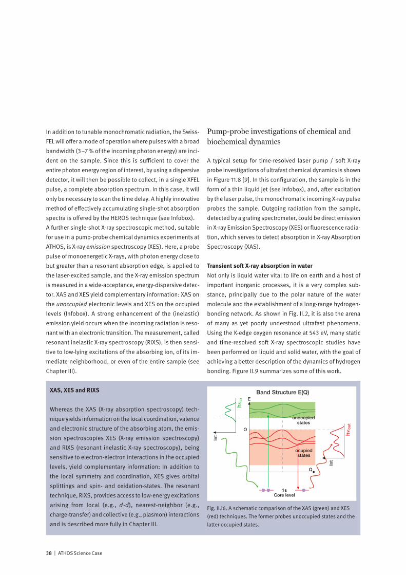
38 | ATHOS Science Case
In addition to tunable monochromatic radiation, the Swiss-FEL will offer a mode of operation where pulses with a broad bandwidth (3–7% of the incoming photon energy) are inci-dent on the sample. Since this is sufficient to cover the entire photon energy region of interest, by using a dispersive detector, it will then be possible to collect, in a single XFEL pulse, a complete absorption spectrum. In this case, it will only be necessary to scan the time delay. A highly innovative method of effectively accumulating single-shot absorption spectra is offered by the HEROS technique (see Infobox).A further single-shot X-ray spectroscopic method, suitable for use in a pump-probe chemical dynamics experiments at ATHOS, is X-ray emission spectroscopy (XES). Here, a probe pulse of monoenergetic X-rays, with photon energy close to but greater than a resonant absorption edge, is applied to the laser-excited sample, and the X-ray emission spectrum is measured in a wide-acceptance, energy-dispersive detec-tor. XAS and XES yield complementary information: XAS on the unoccupied electronic levels and XES on the occupied levels (Infobox). A strong enhancement of the (inelastic) emission yield occurs when the incoming radiation is reso-nant with an electronic transition. The measurement, called resonant inelastic X-ray spectroscopy (RIXS), is then sensi-tive to low-lying excitations of the absorbing ion, of its im-mediate neighborhood, or even of the entire sample (see Chapter III).
Pump-probe investigations of chemical and biochemical dynamics
A typical setup for time-resolved laser pump / soft X-ray probe investigations of ultrafast chemical dynamics is shown in Figure 11.8 [9]. In this configuration, the sample is in the form of a thin liquid jet (see Infobox), and, after excitation by the laser pulse, the monochromatic incoming X-ray pulse probes the sample. Outgoing radiation from the sample, detected by a grating spectrometer, could be direct emission in X-ray Emission Spectroscopy (XES) or fluorescence radia-tion, which serves to detect absorption in X-ray Absorption Spectroscopy (XAS).
Transient soft X-ray absorption in waterNot only is liquid water vital to life on earth and a host of important inorganic processes, it is a very complex sub-stance, principally due to the polar nature of the water molecule and the establishment of a long-range hydrogen-bonding network. As shown in Fig. II.2, it is also the arena of many as yet poorly understood ultrafast phenomena. Using the K-edge oxygen resonance at 543 eV, many static and time-resolved soft X-ray spectroscopic studies have been performed on liquid and solid water, with the goal of achieving a better description of the dynamics of hydrogen bonding. Figure II.9 summarizes some of this work.
XAS, XES and RIXS
Whereas the XAS (X-ray absorption spectroscopy) tech-nique yields information on the local coordination, valence and electronic structure of the absorbing atom, the emis-sion spectroscopies XES (X-ray emission spectroscopy) and RIXS (resonant inelastic X-ray spectroscopy), being sensitive to electron-electron interactions in the occupied levels, yield complementary information: In addition to the local symmetry and coordination, XES gives orbital splittings and spin- and oxidation-states. The resonant technique, RIXS, provides access to low-energy excitations arising from local (e.g., d-d), nearest-neighbor (e.g., charge-transfer) and collective (e.g., plasmon) interactions and is described more fully in Chapter III.
Band Structure E(Q)
1sCore level
E
Q
hνin
hνo
ut
O
ocupiedstates
unocupiedstates
Int
Int
Fig. II.i6. A schematic comparison of the XAS (green) and XES (red) techniques. The former probes unoccupied states and the latter occupied states.
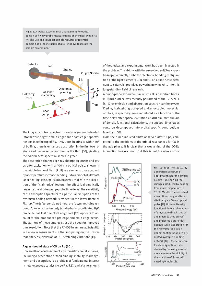
ATHOS Science Case | 39
The X-ray absorption spectrum of water is generally divided into the “pre-edge”, “main-edge” and “post-edge” spectral regions (see the top of Fig. II.9). Upon heating to within 10° of boiling, there is enhanced absorption in the first two re-gions and decreased absorption in the third [10], yielding the “difference” spectrum shown in green.The absorption changes in X-ray absorption 200 ns and 150 ps after excitation with a 400 nm optical pulse, shown in the middle frame of Fig. II.9 [11], are similar to those caused by a temperature increase, leading us to a model of ultrafast laser heating. It is significant, however, that with the excep-tion of the “main edge” feature, the effect is dramatically larger for the shorter pump-probe time delay. The sensitivity of the absorption spectrum to a particular disruption of the hydrogen boding network is evident in the lower frame of Fig. II.9. The defect considered here, the “asymmetric broken donor”, for which a formerly tetrahedrally-coordinated H2O molecule has lost one of its neighbors [12], appears to ac-count for the pronounced pre-edge and main-edge peaks. The authors of these studies stress the need for improved time resolution. Note that the ATHOS beamline at SwissFEL will allow measurements in the sub-ps region, i.e., faster than the 5 ps relaxation of O-H stretching vibrations [11].
A quasi-bound state of CO on Ru (001)How small molecules interact with transition metal surfaces, including a description of their binding, mobility, rearrange-ment and desorption, is a problem of fundamental interest in heterogeneous catalysis (see Fig. II.3), and a large amount
of theoretical and experimental work has been invested in the problem. The ability, with time-resolved soft X-ray spec-troscopy, to directly probe the electronic bonding configura-tion of the light elements C, N and O, on a time scale perti-nent to catalysis, promises powerful new insights into this long-standing field of research.A pump-probe experiment in which CO is desorbed from a Ru (001) surface was recently performed at the LCLS XFEL [8]. X-ray emission and absorption spectra near the oxygen K-edge, highlighting occupied and unoccupied molecular orbitals, respectively, were monitored as a function of the time delay after optical excitation at 400 nm. With the aid of density functional calculations, the spectral lineshapes could be decomposed into orbital-specific contributions (see Fig. II.10).From the pump-induced shifts observed after 12 ps, com-pared to the positions of the orbital resonances for CO in the gas phase, it is clear that a weakening of the CO-Ru interaction has occurred. But this is not the whole story.
Fig. II.8. A typical experimental arrangement for optical pump / soft X-ray probe measurements of chemical dynamics [9]. The use of a liquid jet sample requires differential pumping and the inclusion of a foil window, to isolate the sample environment.
Fig. II.9. Top: The static X-ray absorption spectrum of liquid water, near the oxygen K-edge [10], showing the changes produced by heating from room temperature to 90 °C. Middle: Time-resolved absorption changes after ex-citation by a 400 nm optical pulse [11]. Bottom: Density functional theory calculations of the p-state (black, dotted and green-dashed curves) and projected s-state (dot-dashed curve) absorption for the “asymmetric broken donor” configuration of a dis-rupted hydrogen bonding network [12] – the tetrahedral local configuration is de-stroyed by removing a water molecule from the vicinity of the now three-fold coordi-nated H2O molecule.
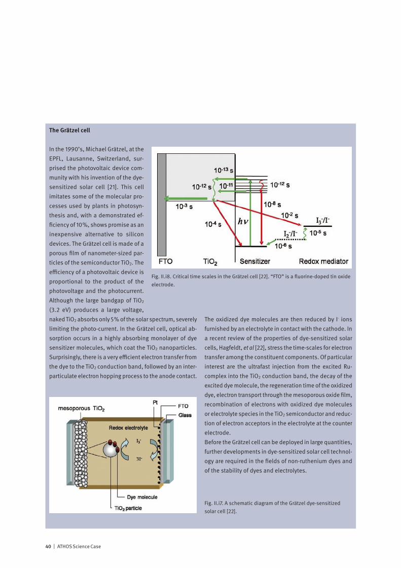
40 | ATHOS Science Case
The Grätzel cell
In the 1990’s, Michael Grätzel, at the EPFL, Lausanne, Switzerland, sur-prised the photovoltaic device com-munity with his invention of the dye-sensitized solar cell [21]. This cell imitates some of the molecular pro-cesses used by plants in photosyn-thesis and, with a demonstrated ef-ficiency of 10%, shows promise as an inexpensive alternative to silicon devices. The Grätzel cell is made of a porous film of nanometer-sized par-ticles of the semiconductor TiO2. The efficiency of a photovoltaic device is proportional to the product of the photovoltage and the photocurrent. Although the large bandgap of TiO2 (3.2 eV) produces a large voltage, naked TiO2 absorbs only 5% of the solar spectrum, severely limiting the photo-current. In the Grätzel cell, optical ab-sorption occurs in a highly absorbing monolayer of dye sensitizer molecules, which coat the TiO2 nanoparticles. Surprisingly, there is a very efficient electron transfer from the dye to the TiO2 conduction band, followed by an inter-particulate electron hopping process to the anode contact.
The oxidized dye molecules are then reduced by I- ions furnished by an electrolyte in contact with the cathode. In a recent review of the properties of dye-sensitized solar cells, Hagfeldt, et al [22], stress the time-scales for electron transfer among the constituent components. Of particular interest are the ultrafast injection from the excited Ru-complex into the TiO2 conduction band, the decay of the excited dye molecule, the regeneration time of the oxidized dye, electron transport through the mesoporous oxide film, recombination of electrons with oxidized dye molecules or electrolyte species in the TiO2 semiconductor and reduc-tion of electron acceptors in the electrolyte at the counter electrode.Before the Grätzel cell can be deployed in large quantities, further developments in dye-sensitized solar cell technol-ogy are required in the fields of non-ruthenium dyes and of the stability of dyes and electrolytes.
Fig. II.i7. A schematic diagram of the Grätzel dye-sensitized solar cell [22].
Fig. II.i8. Critical time scales in the Grätzel cell [22]. “FTO” is a fluorine-doped tin oxide electrode.

ATHOS Science Case | 41
If one follows spectral details, such as the intensity of the dπ component or the energy shift of the 2π* resonance, as a function of pump-probe delay, one sees that a sudden reversal happens at 1 ps (see the top of Fig. II.11).With the aid of density functional calculations of the binding force (Fig. II.11 bottom), the behavior could be interpreted as follows: CO is initially bound in the vertically-oriented “atop” configuration to a single Ru atom. Upon laser excita-tion, hot electrons from the substrate quickly excite a wag-ging motion of the CO, causing an unstable intermediate configuration with increased interaction between CO and the neighboring Ru atoms. Later on, the CO molecule adopts an energetically favorable orientation approximately paral-lel to and at some distance from the surface. This is evidence for a “quasi-bound” state, that had been predicted but never observed. Since the binding energy depends strongly on the molecular orientation, the binding is due to a shallow “entropic barrier” (see also Ch. I).
L-edge spectroscopy of metalloproteinsThe examples given so far of time-resolved soft X-ray spec-troscopy have focused on the K-edge resonance of a light atom (oxygen). Since oxygen is omnipresent in (hydrated) biological systems, if one wants to observe the biochemical action of a particular molecular component, the oxygen signal from the solute or parts of biomolecules not of im-mediate interest will produce a strong background. In the important case of metalloproteins, one concentrates on the local electronic behavior in the vicinity of a transition metal ion. As seen in Fig. 1 of the Introduction, these ions have
characteristic L-edge resonances in the soft X-ray region, accessible with the ATHOS beamline at SwissFEL.A long-standing problem in biochemistry involves the struc-ture and dynamics of the so-called water oxidizing complex (WOC) in the key protein involved in photosynthesis, pho-tosystem II (PSII). Upon photo-triggering, this complex, based on a tightly-bound Mn4OnCa cluster, is known to undergo a cyclic reaction, the Kok cycle, passing sequentially through the oxidation states S0, … S4, and splitting H2O molecules into H+ and O2 (see Fig. II.12). The study of the WOC and PSII is complicated by the difficulty of crystallizing this membrane protein, by its high sensitivity to radiation
Fig. II.10. A comparison of XES and XAS oxygen K-edge spec-tra, taken before and after excitation by a 400 nm optical pulse [8]. Consideration of the orbital resonance energies for gas-phase CO, shown at the top of the figure, demonstrates a pump-induced partial weakening of the CO-Ru interaction.
Fig. II.11. Top: Dependence of two particular features of the XES and XAS spectra, the intensity of the dπ resonance and the energy position of the 2π* resonance, on the pump-probe delay [8]. The observed behaviors, as well as density func-tional calculations (bottom), which include van der Waals in-teractions, are consistent with a prompt strengthening of the CO-Ru interaction up to 1 ps, due to pronounced wagging of the atop-bound CO molecule, followed by a partial weaken-ing of the interaction, attributed to the formation of a quasi-bound state, persisting up to at least 20 ps.
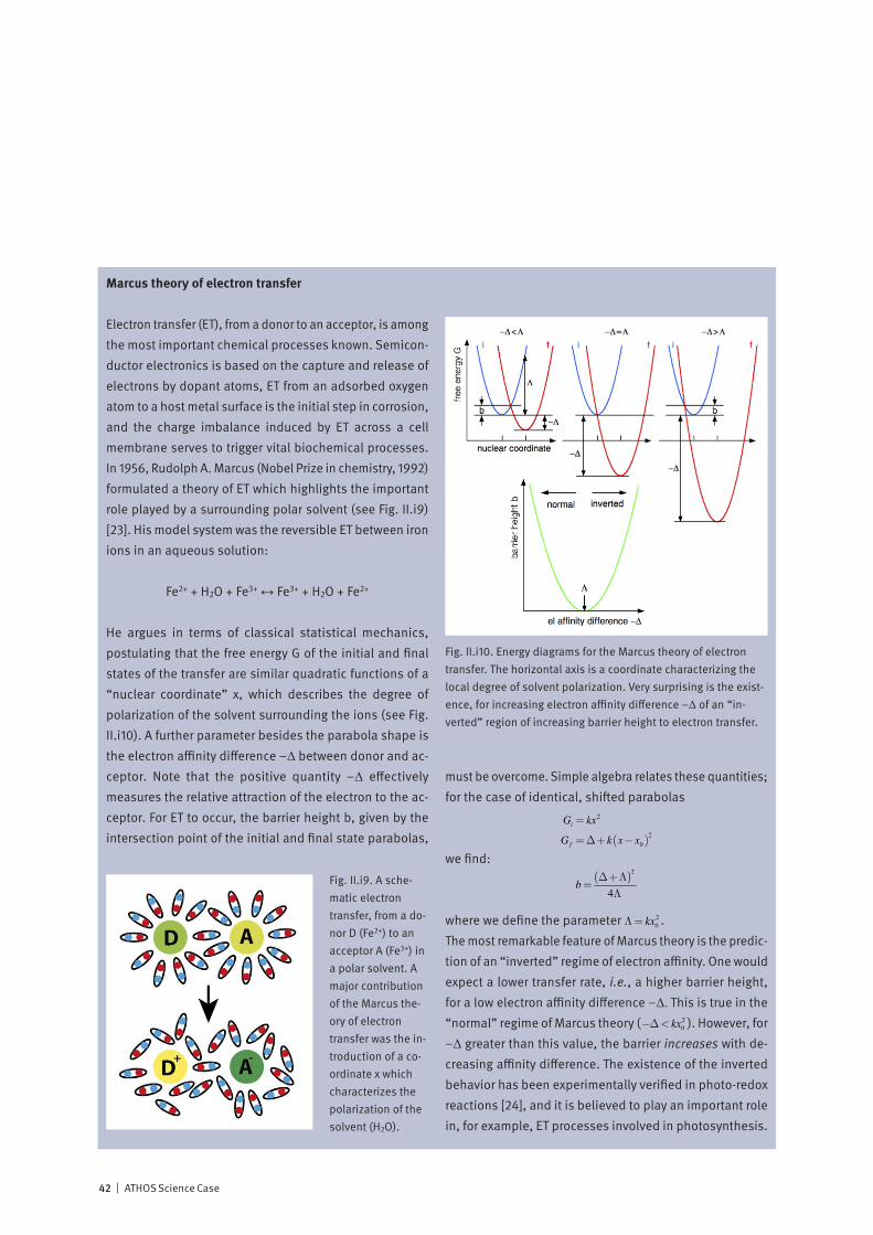
42 | ATHOS Science Case
Marcus theory of electron transfer
Electron transfer (ET), from a donor to an acceptor, is among the most important chemical processes known. Semicon-ductor electronics is based on the capture and release of electrons by dopant atoms, ET from an adsorbed oxygen atom to a host metal surface is the initial step in corrosion, and the charge imbalance induced by ET across a cell membrane serves to trigger vital biochemical processes. In 1956, Rudolph A. Marcus (Nobel Prize in chemistry, 1992) formulated a theory of ET which highlights the important role played by a surrounding polar solvent (see Fig. II.i9) [23]. His model system was the reversible ET between iron ions in an aqueous solution:
Fe2+ + H2O + Fe3+ ↔ Fe3+ + H2O + Fe2+
He argues in terms of classical statistical mechanics, postulating that the free energy G of the initial and final states of the transfer are similar quadratic functions of a “nuclear coordinate” x, which describes the degree of polarization of the solvent surrounding the ions (see Fig. II.i10). A further parameter besides the parabola shape is the electron affinity difference –Δ between donor and ac-ceptor. Note that the positive quantity –Δ effectively measures the relative attraction of the electron to the ac-ceptor. For ET to occur, the barrier height b, given by the intersection point of the initial and final state parabolas,
must be overcome. Simple algebra relates these quantities; for the case of identical, shifted parabolas
.
)
we find:
.
)
where we define the parameter
.
)
.The most remarkable feature of Marcus theory is the predic-tion of an “inverted” regime of electron affinity. One would expect a lower transfer rate, i.e., a higher barrier height, for a low electron affinity difference –Δ. This is true in the “normal” regime of Marcus theory (
.
)). However, for –Δ greater than this value, the barrier increases with de-creasing affinity difference. The existence of the inverted behavior has been experimentally verified in photo-redox reactions [24], and it is believed to play an important role in, for example, ET processes involved in photosynthesis.
Fig. II.i9. A sche-matic electron transfer, from a do-nor D (Fe2+) to an acceptor A (Fe3+) in a polar solvent. A major contribution of the Marcus the-ory of electron transfer was the in-troduction of a co-ordinate x which characterizes the polarization of the solvent (H2O).
Fig. II.i10. Energy diagrams for the Marcus theory of electron transfer. The horizontal axis is a coordinate characterizing the local degree of solvent polarization. Very surprising is the exist-ence, for increasing electron affinity difference –Δ of an “in-verted” region of increasing barrier height to electron transfer.

ATHOS Science Case | 43
damage and by the many possible models for its behavior. Photo-triggered time-resolved soft X-ray spectroscopic meas-urements, in solution, at the Mn L-edge resonance could make a major contribution to the understanding of this important biocomplex, perhaps pointing the way to realizing concepts for artificial photosynthesis.But it is far from trivial to perform L-edge XAS of dilute Mn ions (640-650 eV) in the presence of large amounts of oxy-gen. The reason is that XAS on dilute samples demands detection by partial fluorescence yield, and this requires an analyzing detector which can see the weak Mn fluorescence in the presence of the very intense oxygen K-edge fluores-cence at 525 eV. Consider the emission spectrum of a 500
mM solution of MnCl2 in water measured with a conventional superconducing detector (Fig. II.13, left): the Mn peak is a tiny shoulder on the huge oxygen signal [14]. An analyzer detector is required with a large acceptance and excellent spectral rejection. Such a detector has been realized by Mitzner, et al, based on multiple focusing reflection zone plates, and has been successfully tested at the LCLS XFEL (Fig. II.13, right). The authors have since extended this tech-nology to allow efficient measurements at the biologically interesting concentration level of 20 mM. These develop-ments open the way for the study, using time-resolved soft X-ray spectroscopy, e.g., at the ATHOS beamline of SwissFEL, of critical problems in metalloprotein biochemistry.
Fig. II.12. One of the many structural models for the water-oxi-dizing complex (WOC) in the photosystem II (PSII) membrane protein [13]. The red, black and green dots represent Mn, O and Ca, respectively. At right is a schematic summary of the Kok photo-cycle undergone by the WOC.
Fig. II.13. Left: The emission spectrum of 500 mM MnCl2 in water, measured with a 9-element superconducting detector [14]. The Mn L-edge peak is a tiny shoulder on the dominant oxygen K-edge fluores-cence. Right: An XAS measurement (red curve) of the partial fluorescence yield measured by scanning the energy of the LCLS soft X-ray beam and detecting the fluorescence with a new multi-element reflection zone plate spectrometer. This is compared with the absorption spec-trum of a highly-concentrated solution of Mn measured in transmission mode at a synchrotron (blue) and with theoretical calculations (pink and brown).

44 | ATHOS Science Case
Summary
• The time scales for fast chemical processes in solution span the region from microseconds to femtoseconds – which is well-suited to pump-probe soft X-ray spectroscopic methods at the ATHOS beamline at SwissFEL. An important unsolved problem is determining the rate of electron solvation in water.
• Heterogeneous catalysis, which is of major importance in the chemical industry, can be studied at soft X-ray resonances of the light-atom reacting species. Photo-triggering of catalytic reactions can be accomplished indirectly, by optically exciting hot electrons in the substrate, or directly, by exerting electric forces on polar reactants with intense, few-cycle pulses of terahertz radiation.
• Delivery of chemical samples to the X-ray beam at ATHOS can be accomplished either using reactive species (including catalytic nano-particles) in a thin liquid jet injected into vacuum or in the form of adsorbates on a clean crystalline surface.
• Unoccupied molecular orbitals can be studied at ATHOS using X-ray absorption spectroscopy (XAS). The absorption signal can be measured in transmission, for concentrated samples, or via characteristic fluorescence, for dilute samples. Single-shot measurements, without the need of scanning the incoming X-ray wavelength, can be realized either with the SwissFEL broadband mode and a dispersive detector or with a fixed incoming wavelength using the “HEROS” technique.
• Occupied orbitals are characterized with X-ray emission spectroscopy (XES), which uses a fixed incoming wavelength but which requires a spectral analysis of the emitted radiation. When the incoming photons are resonant with atomic transitions in the sample, the technique is called “resonant inelastic X-ray spectroscopy” (RIXS).
• Examples of initial chemical and biochemical experiments using ultrafast time-resolved soft X-ray spectroscopy are: determining the dynamics of the hydrogen-bonding network in liquid water, providing experimental proof of the existence of a short-lived “quasi-bound” state during the laser-induced desorption of CO from a Ru surface, and following the photo-induced process of water-splitting in the water oxidizing complex in a photosynthetic protein.
ATHOS Science Case | 45
References
[1] Nilsson, A., Nordlund, D., and Ogasawara, H., (private communication).
[2] Ertl, G., “Research with surface science”, Chin. J. Catal. 28, II-V (2007).
[3] BNL, Surface Chemical Dynamics Program, http://www.bnl.gov/chemistry/programs/ Surface_dynamics.asp.
[4] Kimura, T., “Imaging live cell in micro-liquid enclosure by X-ray laser diffraction”, Nature Comm 5, 3052 (2014).
[5] Vos, M. and Van Thor, J., (private communication).[6] Ansari, A., et al., “Protein states and protein quakes,”
Proc. Nat. Acad. Sci. USA 82, 5000-5004 (1985).[7] Zang, C., et al., “Ultrafast protein quake dynamics in
Cytochrome C,” J. Am. Chem. Soc. 131, 2846-2852 (2009).[8] Beye, M., et al., Time Resolved Resonant Inelastic X-ray
Scattering: A Supreme Tool to Understand Dynamics in Solids and Molecules, J. Electron Spectrosc. Relat. Phenom. 188, 172-182 (2013).
[9] Kunnus K., et al., “A setup for resonant inelastic soft x-ray scattering on liquids at free electron laser light sources”, Rev. Sci. Inst. 83, 123109 (2012).
[10] Nilsson A, et al., “Resonant inelastic X-ray scattering of liquid water”, J. Elect. Spect. Rel. Phenom. 188, 84 (2013).
[11] Huse, N., et al., “Probing the hydrogen-bond network of water via time-resolved soft X-ray spectroscopy”, Phys. Chem. Chem. Phys. 11, 3951 (2009).
[12] Cavalleri, M., et al., “The interpretation of X-ray absorption spectra of water and ice”, Chem. Phys. Lett. 364, 363 (2002).
[13] Zein, S., et al., “Focusing the view on nature’s water-splitting catalyst”, Phil. Trans. R. Soc. B, 363, 1167 (2008).
[14] Mitzner, R., et al., “L-edge X-ray absorption spectroscopy of dilute systems relevant to metalloproteins using an X-ray free-electron laser”, J. Phys. Chem. Lett. 4, 3641 (2013).
[15] Ogasawara, H., Nordlund, D., and Nilsson, A.“Ultrafast coherent control and characterization of surface reactions using FELS,” in Proceedings of the 27th International Free Electron Laser Conference (JACoW/eConf C0508213, Stanford, California, USA, 2005).
[16] Sussman, B. J., Townsend, D., Ivanov, M. Y., and Stolow, A., “Dynamic Stark control of photochemical processes,” Science 314, 278-281 (2006).
[17] Winter, B. and Faubel, M., “Photoemission from liquid aqueous solutions,” Chem. Rev. 106, 1176-1211 (2006).
[18] Aziz, E. F., (private communication).[19] Szlachetko, J., et al., “High energy resolution off-resonant
spectroscopy at sub-second time resolution: (Pt(acac)2) decomposition”, Chem. Commun. 48, 10898–10900, (2012).
[20] Tulkki J. and Åberg T, “Behaviour of Raman resonance scattering across the K x-ray absorption edge”, J. Phys. B: At. Mol. Phys. 15, L435-L440 (1982).
[21] O'Regan, B. and Grätzel, M., “A low-cost, high-efficiency solar cell based on dye-sensitized colloidal TiO2 films”, Nature 353, 737-740 (1991).
[22] Hagfeldt, A., “Dye-Sensitized Solar Cells”, Chem. Rev. 110, 6595–6663 (2010).
[23] Marcus, R.A. "On the Theory of Oxidation-Reduction Reactions Involving Electron Transfer. I". J. Chem. Phys. 24 966 (1956).
[24] Miller, J.R., Calcaterra, L.T. and Closs, G.L., „Intramolecular Long-Distance Electron Transfer in Radical Anions. The Effects of Free Energy and Solvent on the Reaction Rates”, J. Am. Chem. Soc. 106, 3047-3049 (1984).
46 | ATHOS Science Case
“Electron correlation” is a dominant theme in condensed matter science, mani-festing itself in, e.g., “metal-insulator transitions” (MIT), “high-temperature superconductivity” (HTS) and “colossal magneto-resistance” (CMR). On the microscopic scale, one speaks of the charge (C), spin (S) and orbital (O) degrees of freedom, each of which may show short- or long-range order, and each of which may exchange energy with the others and with the crystal lattice (L) (see Fig. III.1). Important correlation effects can occur in systems with partially-filled electron shells, such as those of 3d-transition metal ions, with anisotropic, quasi-localized character. Vast amounts of experimental and theoretical work have been published on electron correlation, triggered largely by the discovery of HTS in 1986 [2]. Phase diagrams of many interesting materials have been in-vestigated in detail, and numerous theories of the microscopic charge-spin-or-bital-lattice interactions have been proposed. Much has been achieved, but much is still unclear. There is increasing evidence of the importance of nanoscale inhomogeneities and fast fluctuations in correlated electron materials – indicat-ing the important role that the ATHOS beamline at SwissFEL will play. Furthermore, it has been suggested that the chicken-or-egg problem, of determining the cause and effect relationships among the C, S, O and L subsystems, may best be ap-proached with pump-probe time-resolved spectroscopy: one pumps energy into a particular degree of freedom and measures the time required for a response to appear in the others.
III. Time-Resolved Spectroscopy of Correlated Electron MaterialsMapping the flow of energy among strongly-coupled degrees of freedom
• Correlated electron phases
• X-ray methods in correlated electron science
• The origin of the metal-insulator transition in TaS2
• Further pump-probe experiments
• Complexity in correlated electron materials

ATHOS Science Case | 47
Multiferroic materials
Fig. III.i1. The multiferroic material RbFe(MoO4)2.
Orderings that can be switched between and “up” and “down” states are examples of parameters called ferroic. If a material has simultaneously two ferroic order paramat-ers of different types, then it is called multiferroic. This definition has been somewhat relaxed in the past few years, and it has now become customary to call any mate-
rial multiferroic that shows spontaneous magnetic order and ferroelectricity [21]. An example is when a material has a spontaneous dipole moment and antiferromagnetic or-der. Because multiple order parameters are almost always coupled, multiferroic materials hold the promise that the electric dipole moment can be manipulated magnetically, or that ferromagnetic magnetization can be manipulated electrically, with exciting possibilities for novel device applications involving ultrafast switching. There are different mechanisms that can lead to the simul-taneous presence of ferroelectricy and magnetic order. One of the simplest is when ferroelectricity emerges directly from magnetic order. This can happen when magnetic order breaks the inversion symmetry, allowing a switchable electric polarization to occur. There are other mechanisms, such as spiral driven ferroelectricity, which are as yet not fully understood. A recent puzzling case are materials in which ferroelectricity arises from charge frustration which is coupled with magnetism (see Fig. III.i1). This can lead to a large electric polarization and strong coupling effects at high temperature. There are only few such electronic fer-roelectrics known to date, and their physics is presently under intense investigation.
Chimera
Spin
Charge
Orbital
Lattice
HTS CMR
T THigh TemperatureSuperconductivity
RR B=0
B>0
ColossalMagneto-Resistance
MIT
TMetal-to-Insulator
Transition
R
Fig. III.1. a) Three macroscopic manifestations of correlated electrons, with strong potential for important applications. b) The Charge-Spin-Orbital-Lattice “Chimera” of correlated electron science [1], which emphasizers the interrelated degrees of freedom. The Chimera is a beast from Greek mythology.
b)a)
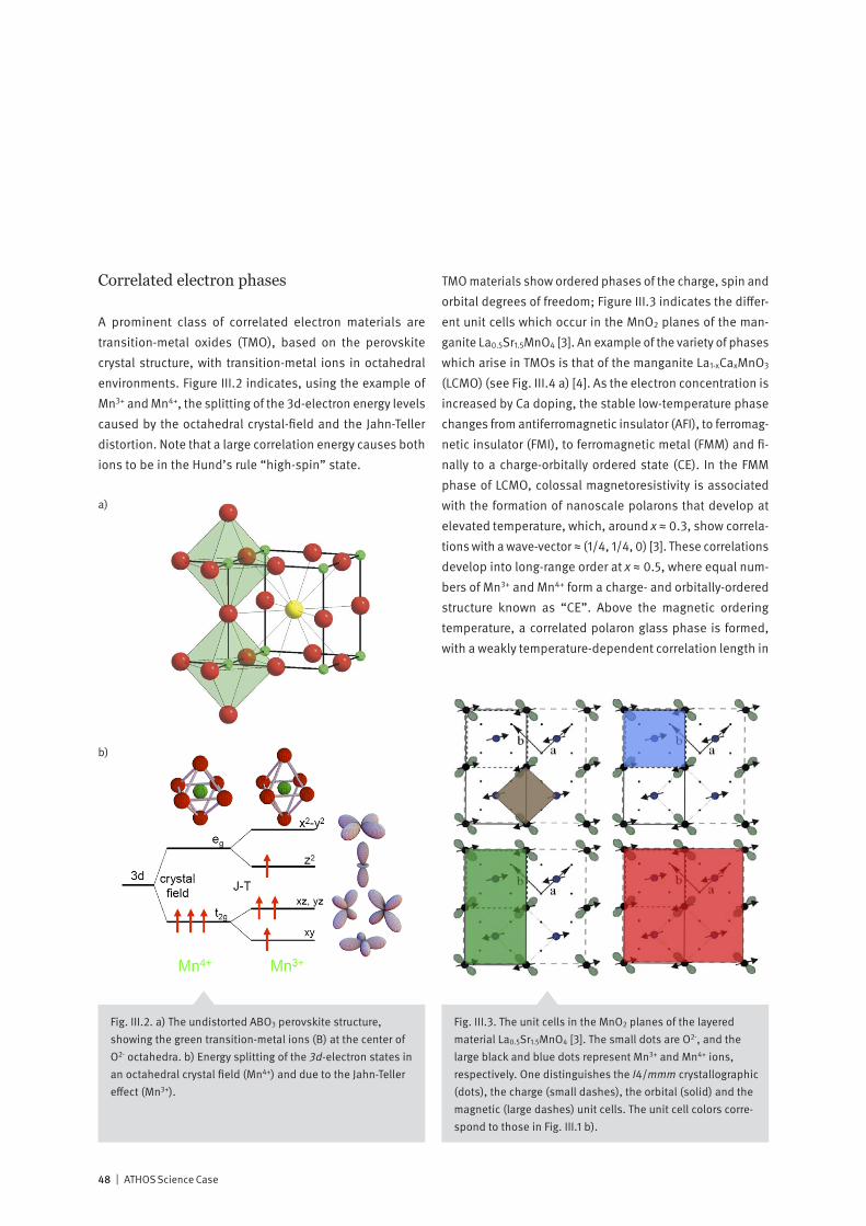
48 | ATHOS Science Case
Correlated electron phases
A prominent class of correlated electron materials are transition-metal oxides (TMO), based on the perovskite crystal structure, with transition-metal ions in octahedral environments. Figure III.2 indicates, using the example of Mn3+ and Mn4+, the splitting of the 3d-electron energy levels caused by the octahedral crystal-field and the Jahn-Teller distortion. Note that a large correlation energy causes both ions to be in the Hund’s rule “high-spin” state.
TMO materials show ordered phases of the charge, spin and orbital degrees of freedom; Figure III.3 indicates the differ-ent unit cells which occur in the MnO2 planes of the man-ganite La0.5Sr1.5MnO4 [3]. An example of the variety of phases which arise in TMOs is that of the manganite La1-xCaxMnO3 (LCMO) (see Fig. III.4 a) [4]. As the electron concentration is increased by Ca doping, the stable low-temperature phase changes from antiferromagnetic insulator (AFI), to ferromag-netic insulator (FMI), to ferromagnetic metal (FMM) and fi-nally to a charge-orbitally ordered state (CE). In the FMM phase of LCMO, colossal magnetoresistivity is associated with the formation of nanoscale polarons that develop at elevated temperature, which, around x ≈ 0.3, show correla-tions with a wave-vector ≈ (1/4, 1/4, 0) [3]. These correlations develop into long-range order at x ≈ 0.5, where equal num-bers of Mn3+ and Mn4+ form a charge- and orbitally-ordered structure known as “CE”. Above the magnetic ordering temperature, a correlated polaron glass phase is formed, with a weakly temperature-dependent correlation length in
Fig. III.3. The unit cells in the MnO2 planes of the layered material La0.5Sr1.5MnO4 [3]. The small dots are O2-, and the large black and blue dots represent Mn3+ and Mn4+ ions, respectively. One distinguishes the I4/mmm crystallographic (dots), the charge (small dashes), the orbital (solid) and the magnetic (large dashes) unit cells. The unit cell colors corre-spond to those in Fig. III.1 b).
Fig. III.2. a) The undistorted ABO3 perovskite structure, showing the green transition-metal ions (B) at the center of O2- octahedra. b) Energy splitting of the 3d-electron states in an octahedral crystal field (Mn4+) and due to the Jahn-Teller effect (Mn3+).
a)
b)
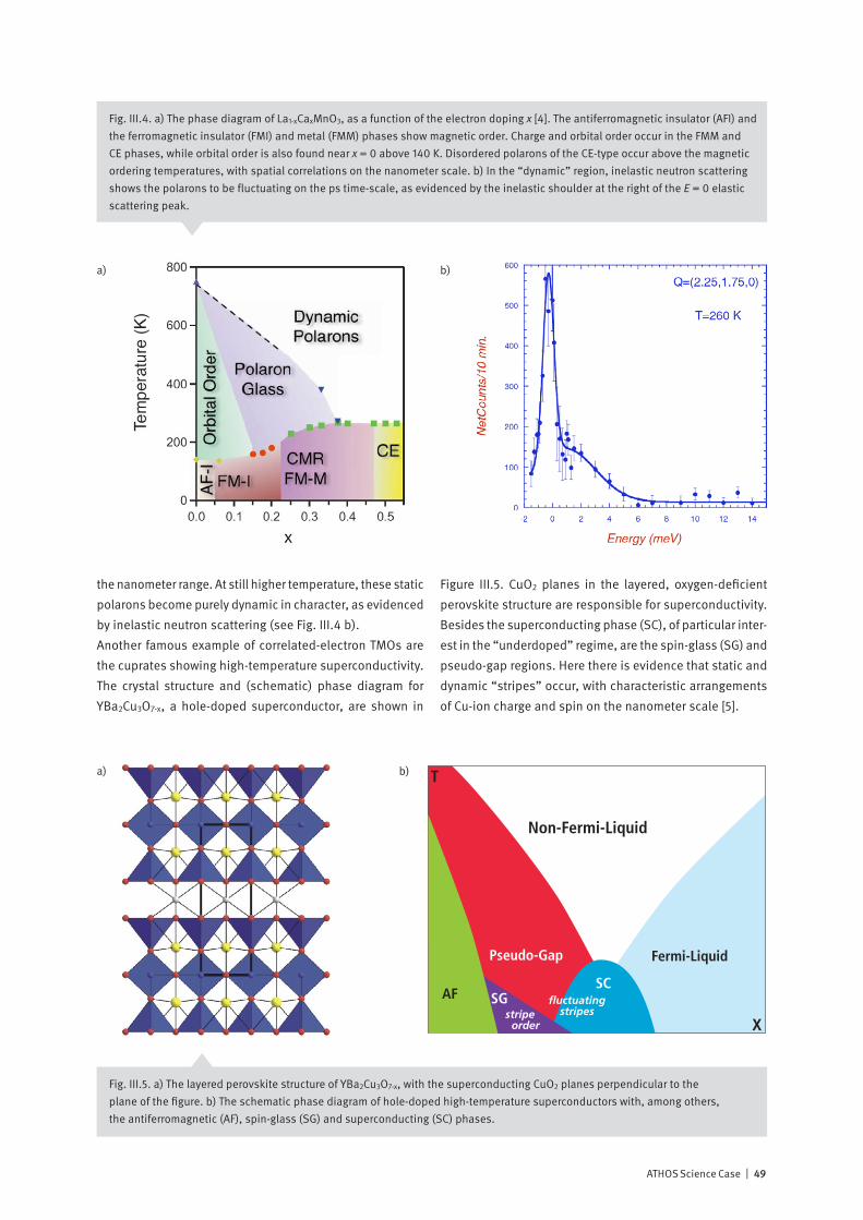
ATHOS Science Case | 49
the nanometer range. At still higher temperature, these static polarons become purely dynamic in character, as evidenced by inelastic neutron scattering (see Fig. III.4 b).Another famous example of correlated-electron TMOs are the cuprates showing high-temperature superconductivity. The crystal structure and (schematic) phase diagram for YBa2Cu3O7-x, a hole-doped superconductor, are shown in
Figure III.5. CuO2 planes in the layered, oxygen-deficient perovskite structure are responsible for superconductivity. Besides the superconducting phase (SC), of particular inter-est in the “underdoped” regime, are the spin-glass (SG) and pseudo-gap regions. Here there is evidence that static and dynamic “stripes” occur, with characteristic arrangements of Cu-ion charge and spin on the nanometer scale [5].
Non-Fermi-Liquid
Fermi-LiquidPseudo-Gap
AFSC
SG
X
T
fluctuatingstripesstripe
order
Fig. III.4. a) The phase diagram of La1-xCaxMnO3, as a function of the electron doping x [4]. The antiferromagnetic insulator (AFI) and the ferromagnetic insulator (FMI) and metal (FMM) phases show magnetic order. Charge and orbital order occur in the FMM and CE phases, while orbital order is also found near x = 0 above 140 K. Disordered polarons of the CE-type occur above the magnetic ordering temperatures, with spatial correlations on the nanometer scale. b) In the “dynamic” region, inelastic neutron scattering shows the polarons to be fluctuating on the ps time-scale, as evidenced by the inelastic shoulder at the right of the E = 0 elastic scattering peak.
Fig. III.5. a) The layered perovskite structure of YBa2Cu3O7-x, with the superconducting CuO2 planes perpendicular to the plane of the figure. b) The schematic phase diagram of hole-doped high-temperature superconductors with, among others, the antiferromagnetic (AF), spin-glass (SG) and superconducting (SC) phases.
a)
a)
b)
b)

50 | ATHOS Science Case
X-ray methods in correlated electron science
The relevance for correlated-electron materials of ps dynam-ics at the nanoscale, together with strong interaction of X-ray photons with all four of the C-S-O-L degrees of freedom, promises important applications of the ATHOS beamline at SwissFEL. To begin the discussion of relevant X-ray tech-niques, we consider the Hamiltonian describing an X-ray photon field interacting with the electrons in the sample [6, 7]. For the moment, we treat a single free electron, without spin:
�
H = p – e
A ( )2
2m+ H radiation,
where
�
H radiation = ∑e , k vk� ( a
e k
†� ae k
+ 1
2) describes photons in
the radiation field, with wavevector
�
k and polarization ε.
Expanding the expression for H, we obtain:
H = Helectron + H interaction + H radiation
Helectron =p2
2m
H interaction =e2 A2
2m–
e
A • p m
≡ H1 + H2
The interaction Hamiltonian, Hinteraction, is responsible for producing a transition from an intial state |i〉 to a final state | f 〉 of the combined system of X-rays and sample. According to Fermi’s Golden Rule, the transition rate is given by:
!
w =2"
hf H
1i +
f H2n n H
2i
E0# En + h$kn
%2
& h$k # h$k'( ) # E f # E0( )( )
Here we are interested in “photon-in” (k) to “photon-out” (k’) transitions – thus we include only those terms which are quadratic in the vector potential A. We disregard the linear terms, which are responsible for photoemission. The transition rate is proportional to the square of the “scatter-ing factor”, w ∝
�
S Q ,v( ) 2
, which, in turn is a function of the momentum and energy transfers
�
Q = k ' – k and ω = ωk’–ωk.
Consider now the following cases:
X-ray diffractionIf the photon energy ωk is much larger than the excitation energies En-E0 of the system, we need only consider the first matrix element in the expression for w:
Fig. III.6. a) The resonant elastic scattering process, indicating a virtual transition from an occupied core state (blue) to an unoccupied intermediate valence state (red) [8]. b) A charge-dependent shift in the core-level energy shifts the energy-dependent scattering profile, providing contrast for charge-ordering [9].
a) b)

ATHOS Science Case | 51
�
f H1 i ∝
�
jS 0ei
Q • r j 0 = S
Q ,0( )� = F
Q ( )
where |0〉 is the ground-state of the system, and where we now sum over all the electrons, with coordinates
�
r j . For a
crystalline sample, the scattering factor
�
F
Q ( ) , is written
�
F Q ( ) =
l ,m,nS ei
Q • R lmn
i =1
I
Sei
Q • r i fi
Q ( ) ,
i.e., as the product of a lattice sum over the unit cells and a “structure factor” sum over the l atoms per unit cell. The quantity
�
fi
Q ( ) is known as the atomic scattering factor. For
a perfect crystal, the lattice sum dictates that F is non-zero only if
�
Q =
G hkl , a reciprocal lattice vector. This is the condi-
tion for Bragg scattering, which, using the relations
�
Q =4p sinu
l and
�
G =2p
d , can be expressed as Bragg’s law:
�
l = 2d sinu . We thus see that diffraction at the Bragg angle θ is possible when the X-ray wavelength λ is shorter than twice the lattice-plane spacing (2d). The scattered intensity at the Bragg condition is proportional to
�
F Q ( ) 2
. The sen-sitivity of the Bragg condition to the lattice parameters im-plies that the diffraction of short X-ray pulses can be used to directly observe lattice phonons.
Soft X-ray resonant diffractionIf the incoming photon energy lies close to an atomic absorp-tion edge, it is the second-order contribution from H2 which dominates the scattering rate. The case of elastic scattering, ωk’–ωk = 0, is treated via an energy-dependent correction to the atomic scattering factor:
�
fi
Q ( ) ⇒
�
fi
Q ,v( ) = fi
Q ( ) + Dfi
Q ,v( ) ,
where the correction term obeys:
�
Dfi ∝
�
nS
0 e • r ei k • r n n
e '• r ei k ' • r 0
vk – En – E0( ) – iG
We see that the scattering is sensitive to the electronic structure of the ground- and intermediate states and to the
polarization of the incoming and outgoing photons (see Fig. III.6 a). The existence of a “core-hole” in the intermediate state is responsible for introducing the linewidth parameter Γ, representing the lifetime of the state |n>.For soft X-rays, where the photon wave-vector k is signifi-cantly larger than the atomic dimensions, one can expand the exponentials into dipole, quadrupole and octupole terms:
�
0 e • r ei k • r n ≈ 0
e • r n + i 0
e • r ( ) k •
r ( ) n – 0
e • r ( ) k •
r ( )2
n
The product of two such matrix elements yields a hierarchy of tensorial terms: dipole-dipole (rank 2), dipole-quadrupole (rank 3), quadrupole-quadrupole (rank 4), etc. These tenso-rial components can be enhanced by a suitable choice of polarizations and scattering vector.In TMOs, interesting resonances are the L2 and L3 transition-metal edges, which connect filled 2p and unfilled 3d states. The corresponding photon wavelength, approximately one nm, allows the observation of resonant soft-X-ray diffraction, and the dependence of the matrix elements on valence-band electronic structure produces superstructure Bragg reflec-tions, corresponding, for example, to orbital-ordering in the correlated-electron material. And when circularly-polarized X-rays are used, XMCD-contrast (see Chapter I) makes mag-netic order visible. Finally, a charge-dependence of the initial core level shifts the energy-dependent resonant scattering profile (see Fig. III.6 b), providing a charge-order contrast.One should note that soft-X-ray resonant diffraction is not easy: it requires scanning of the incoming photon energy, a multi-axis diffractometer in vacuum, and perhaps polari-zation-analysis of the scattered beam. With the ATHOS beamline at SwissFEL, a pump-probe resonant diffraction experiment can follow, for example, the melting of orbital order by a laser pump pulse and its recovery at later times. Its short pulses and flexible energy tuning, particularly near 1 nm wavelength, make ATHOS an ideal source for such investigations of TMO correlated electron materials. A par-ticularly interesting application of pump-probe resonant elastic scattering at ATHOS would be the time-resolved study, at the nanometer scale, of so-called “orbitons”, wave-like excitations of the orbitally-ordered phase, in manganites (see Fig. III.7).
Fig. III.7. The proposed structure of an “orbiton”, a wave-like excitation of the orbitally-ordered state in manganites. Optical pump-probe experiments provide evidence of its existence, with an oscilla-tion period in the range of 10–50 ps [10]; resonant diffraction at the ATHOS beamline at SwissFEL would allow its detailed study at the nanoscale.

52 | ATHOS Science Case
Resonant inelastic X-ray scattering (RIXS)We now lift the restriction to elastic scattering, by allowingω = ωk’–ωk to be non-zero, requiring, in general, energy analysis of the scattered photons. A schematic of the RIXS process is shown in Figure III.8.
The scattering rate is now given by:
�
w = 2p
∑
f∑n
f H2 n n H2 i
E0 - En + vk + iG�
2
d vk - vk '( ) – E f – Ei( )( )� .
Note the following features: a) The sensitivity to photon polarization and valence electronic states seen in resonant elastic scattering is also present for RIXS. b) Although there exists a (virtual) core-hole in the intermediate state, evi-denced by the Γ-term in the denominator, because there is no hole in the final state, the ωκ’ resolution of RIXS can in principle be infinitely good – as evidenced by the energy δ-function. c) Low-energy collective excitations, such as phonons, plasmons, spinwaves, etc., of the sample are accessible with RIXS, since what is measured is the energy difference between the incoming and outgoing photons. And since two photons are involved, the dipole selection
rule Δl=±1 does not apply, such that a d→d transition can be observed (see Fig. III.9 a). d) Although performed at resonance, RIXS is a low-efficiency process: In resonant elastic scattering, the excitation of each of the N scattering atoms can be coherently added, since there is a unique final
A single-shot RIXS spectrometer
When performing resonant inelastic X-ray scattering (RIXS), the scattered intensity as a function of outgoing photon energy Eout = k’ is normally acquired for particular set-tings of the incoming energy E in = k by the monochroma-tor. This is a procedure which is incompatible with single-shot operation at the SwissFEL. One would like to instantaneously obtain a two-dimensional plot of the scattered intensity as a function of Ein, Eout.A method of performing single-shot RIXS has been pro-posed by V. Strocov [22] (see Fig. III.i2). The SwissFEL pulse is dispersed vertically by a monochromator (upper right in the figure) and brought to a line focus on the (homogene-ous) sample. Scattered light corresponding to the various incoming photon energies is then focused to a vertical line and dispersed in Eout horizontally onto a CCD detector. The result is the desired two-dimensional plot.
Fig. III.i2. Proposal for a doubly-dispersive RIXS spectrometer, suitable for use at the SwissFEL [22]. Advantages of this design include higher efficiency and compatibility with single-shot operation. The “VLS grating” has variable line spacing.
Fig. III.8. A schematic of the resonant inelastic X-ray scatter-ing (RIXS) process.
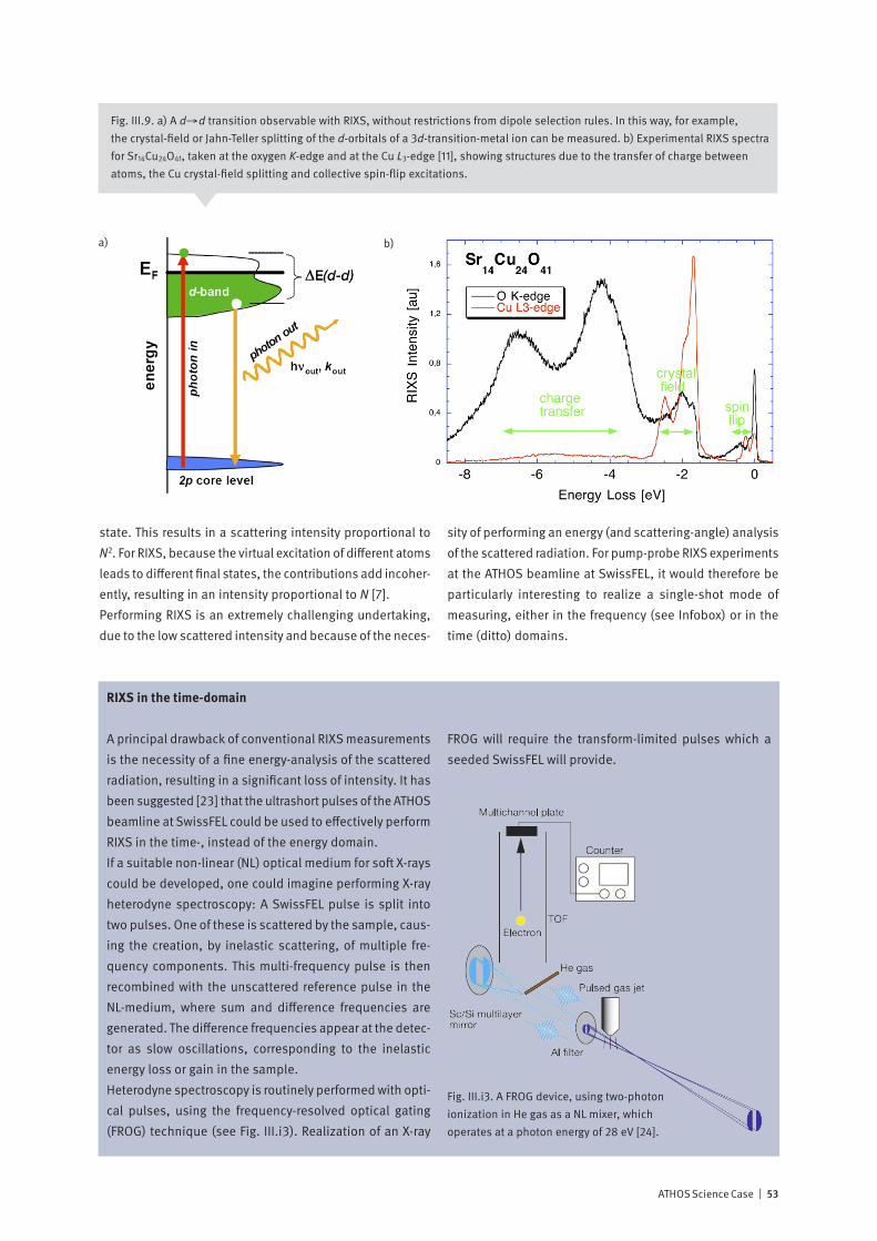
ATHOS Science Case | 53
state. This results in a scattering intensity proportional to N2. For RIXS, because the virtual excitation of different atoms leads to different final states, the contributions add incoher-ently, resulting in an intensity proportional to N [7].Performing RIXS is an extremely challenging undertaking, due to the low scattered intensity and because of the neces-
sity of performing an energy (and scattering-angle) analysis of the scattered radiation. For pump-probe RIXS experiments at the ATHOS beamline at SwissFEL, it would therefore be particularly interesting to realize a single-shot mode of measuring, either in the frequency (see Infobox) or in the time (ditto) domains.
RIXS in the time-domain
A principal drawback of conventional RIXS measurements is the necessity of a fine energy-analysis of the scattered radiation, resulting in a significant loss of intensity. It has been suggested [23] that the ultrashort pulses of the ATHOS beamline at SwissFEL could be used to effectively perform RIXS in the time-, instead of the energy domain. If a suitable non-linear (NL) optical medium for soft X-rays could be developed, one could imagine performing X-ray heterodyne spectroscopy: A SwissFEL pulse is split into two pulses. One of these is scattered by the sample, caus-ing the creation, by inelastic scattering, of multiple fre-quency components. This multi-frequency pulse is then recombined with the unscattered reference pulse in the NL-medium, where sum and difference frequencies are generated. The difference frequencies appear at the detec-tor as slow oscillations, corresponding to the inelastic energy loss or gain in the sample. Heterodyne spectroscopy is routinely performed with opti-cal pulses, using the frequency-resolved optical gating (FROG) technique (see Fig. III.i3). Realization of an X-ray
FROG will require the transform-limited pulses which a seeded SwissFEL will provide.
a) b)
Fig. III.9. a) A d→d transition observable with RIXS, without restrictions from dipole selection rules. In this way, for example, the crystal-field or Jahn-Teller splitting of the d-orbitals of a 3d-transition-metal ion can be measured. b) Experimental RIXS spectra for Sr14Cu24O41, taken at the oxygen K-edge and at the Cu L3-edge [11], showing structures due to the transfer of charge between atoms, the Cu crystal-field splitting and collective spin-flip excitations.
Fig. III.i3. A FROG device, using two-photon ionization in He gas as a NL mixer, which operates at a photon energy of 28 eV [24].
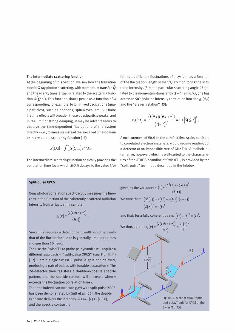
54 | ATHOS Science Case
The intermediate scattering functionAt the beginning of this Section, we saw how the transition rate for X-ray photon scattering, with momentum transfer
�
Q
and the energy transfer ω, is related to the scattering func-tion
�
S Q ,v( ) . This function shows peaks as a function of ω
corresponding, for example, to long-lived oscillations (qua-siparticles), such as phonons, spin-waves, etc. But finite lifetime effects will broaden these quasiparticle peaks, and in the limit of strong damping, it may be advantageous to observe the time-dependent fluctuations of the system directly – i.e., to measure instead the so-called time-domain or intermediate scattering function [12]:
S(Q→
,t) = ∫∞
-∞S(Q→
,ω)eiωtdω.
The intermediate scattering function basically provides the correlation time (over which S(Q,t) decays to the value 1/e)
for the equilibrium fluctuations of a system, as a function of the fluctuation length scale 1/Q. By monitoring the scat-tered intensity I(θ,t) at a particular scattering angle 2θ (re-lated to the momentum-transfer by Q = 4π sin θ/λ), one has access to S(Q,t) via the intensity correlation function g2( θ,t) and the “Siegert relation” [13]:
�
g2 u, t( )
≡
�
I u, t( )I u, t + t( )I u, t( ) 2
= 1+ S Q , t( ) 2
.
A measurement of I(θ,t) on the ultrafast time scale, pertinent to correlated electron materials, would require reading out a detector at an impossible rate of GHz-THz. A realistic al-ternative, however, which is well-suited to the characteris-tics of the ATHOS beamline at SwissFEL, is provided by the “split-pulse” technique described in the Infobox.
Split-pulse XPCS
X-ray photon correlation spectroscopy measures the time-correlation function of the coherently-scattered radiation intensity from a fluctuating sample:
�
g2 t( ) =I t( )I t + t( )
I t( ) 2
.
Since this requires a detector bandwidth which exceeds that of the fluctuations, one is generally limited to times τ longer than 10 nsec.The use the SwissFEL to probe ps-dynamics will require a different approach – “split-pulse XPCS” (see Fig. III.i4) [12]. Here a single SwissFEL pulse is split and delayed, producing a pair of pulses with tunable separation τ. The 2d-detector then registers a double-exposure speckle pattern, and the speckle contrast will decrease when τ exceeds the fluctuation correlation time τc. That one indeed can measure g2(τ) with split-pulse XPCS has been demonstrated by Gutt et al. [26]: The double exposure delivers the intensity
�
S t( ) = I t( ) + I t + t( ) , and the speckle contrast is
given by the variance:
�
c2 t( ) ≡
�
S 2 t( ) – S t( ) 2
S t( ) 2
We note that:
�
S 2 t( ) = 2 I 2 + 2 I t( )I t + t( )S t( ) 2
= 4 I2
and that, for a fully coherent beam,
�
I 2 – I2
= I2 .
We thus obtain:
�
c2 t( ) =I t( )I t + t( )
2 I2
=g2 t( )
2
.
Fig. III.i4. A conceptual “split- and-delay” unit for XPCS at the SwissFEL [25].
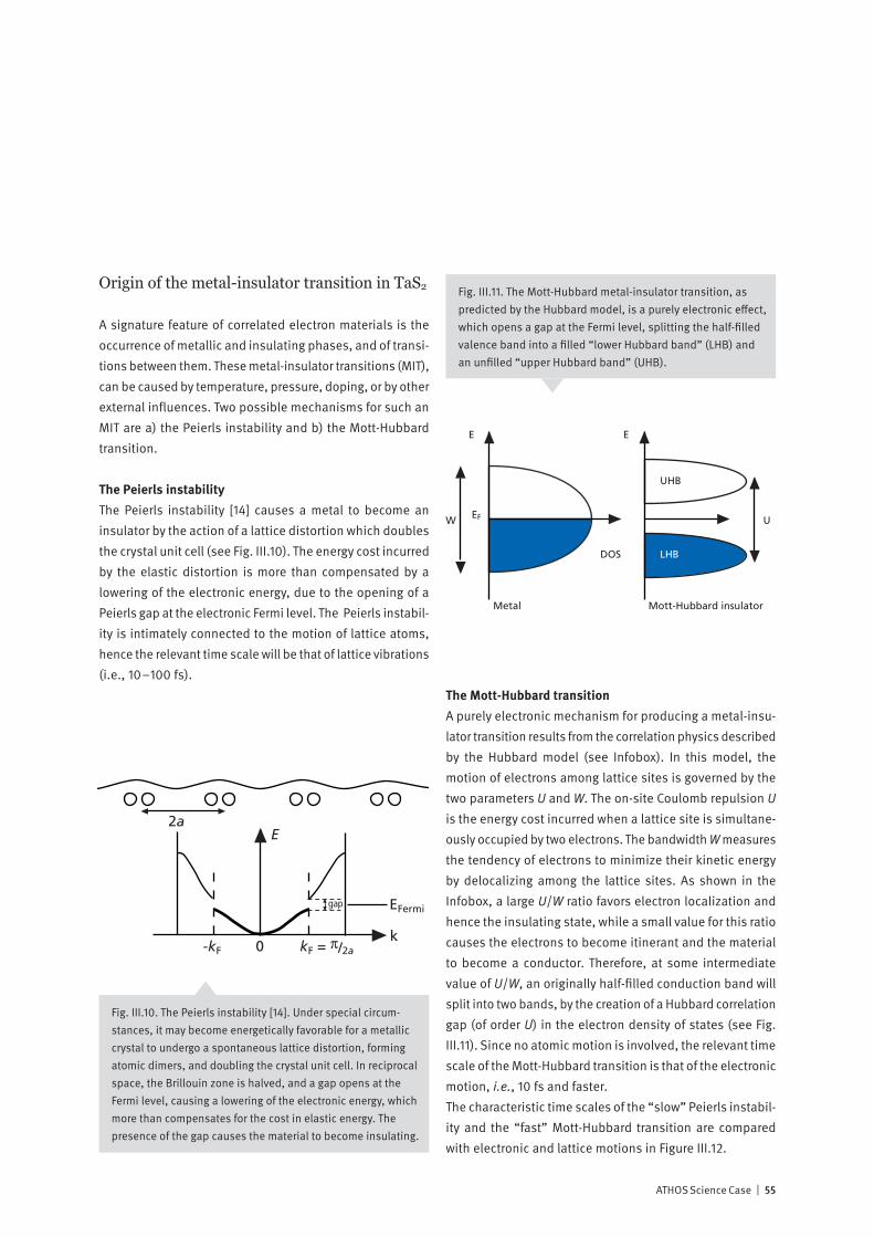
ATHOS Science Case | 55
Origin of the metal-insulator transition in TaS2
A signature feature of correlated electron materials is the occurrence of metallic and insulating phases, and of transi-tions between them. These metal-insulator transitions (MIT), can be caused by temperature, pressure, doping, or by other external influences. Two possible mechanisms for such an MIT are a) the Peierls instability and b) the Mott-Hubbard transition.
The Peierls instabilityThe Peierls instability [14] causes a metal to become an insulator by the action of a lattice distortion which doubles the crystal unit cell (see Fig. III.10). The energy cost incurred by the elastic distortion is more than compensated by a lowering of the electronic energy, due to the opening of a Peierls gap at the electronic Fermi level. The Peierls instabil-ity is intimately connected to the motion of lattice atoms, hence the relevant time scale will be that of lattice vibrations (i.e., 10–100 fs).
The Mott-Hubbard transitionA purely electronic mechanism for producing a metal-insu-lator transition results from the correlation physics described by the Hubbard model (see Infobox). In this model, the motion of electrons among lattice sites is governed by the two parameters U and W. The on-site Coulomb repulsion U is the energy cost incurred when a lattice site is simultane-ously occupied by two electrons. The bandwidth W measures the tendency of electrons to minimize their kinetic energy by delocalizing among the lattice sites. As shown in the Infobox, a large U/W ratio favors electron localization and hence the insulating state, while a small value for this ratio causes the electrons to become itinerant and the material to become a conductor. Therefore, at some intermediate value of U/W, an originally half-filled conduction band will split into two bands, by the creation of a Hubbard correlation gap (of order U) in the electron density of states (see Fig. III.11). Since no atomic motion is involved, the relevant time scale of the Mott-Hubbard transition is that of the electronic motion, i.e., 10 fs and faster.The characteristic time scales of the “slow” Peierls instabil-ity and the “fast” Mott-Hubbard transition are compared with electronic and lattice motions in Figure III.12.
2aE
-kF 0 kF = π/2ak
gap EFermi
E
EF UW
DOS
Metal Mott-Hubbard insulator
E
UHB
LHB
Fig. III.11. The Mott-Hubbard metal-insulator transition, as predicted by the Hubbard model, is a purely electronic effect, which opens a gap at the Fermi level, splitting the half-filled valence band into a filled “lower Hubbard band” (LHB) and an unfilled “upper Hubbard band” (UHB).
Fig. III.10. The Peierls instability [14]. Under special circum-stances, it may become energetically favorable for a metallic crystal to undergo a spontaneous lattice distortion, forming atomic dimers, and doubling the crystal unit cell. In reciprocal space, the Brillouin zone is halved, and a gap opens at the Fermi level, causing a lowering of the electronic energy, which more than compensates for the cost in elastic energy. The presence of the gap causes the material to become insulating.
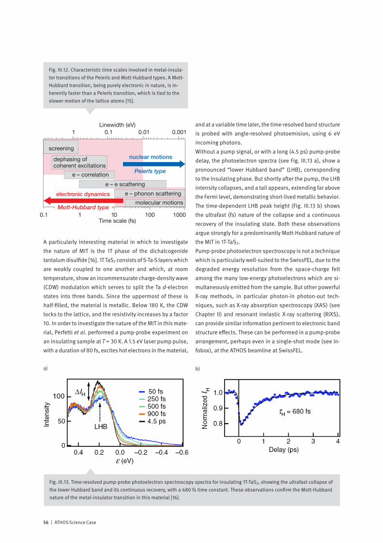
56 | ATHOS Science Case
A particularly interesting material in which to investigate the nature of MIT is the 1T phase of the dichalcogenide tantalum disulfide [16]. 1T TaS2 consists of S-Ta-S layers which are weakly coupled to one another and which, at room temperature, show an incommensurate charge-density wave (CDW) modulation which serves to split the Ta d-electron states into three bands. Since the uppermost of these is half-filled, the material is metallic. Below 180 K, the CDW locks to the lattice, and the resistivity increases by a factor 10. In order to investigate the nature of the MIT in this mate-rial, Perfetti et al. performed a pump-probe experiment on an insulating sample at T = 30 K. A 1.5 eV laser pump pulse, with a duration of 80 fs, excites hot electrons in the material,
and at a variable time later, the time-resolved band structure is probed with angle-resolved photoemision, using 6 eV incoming photons.Without a pump signal, or with a long (4.5 ps) pump-probe delay, the photoelectron spectra (see Fig. III.13 a), show a pronounced “lower Hubbard band” (LHB), corresponding to the insulating phase. But shortly after the pump, the LHB intensity collapses, and a tail appears, extending far above the Fermi level, demonstrating short-lived metallic behavior. The time-dependent LHB peak height (Fig. III.13 b) shows the ultrafast (fs) nature of the collapse and a continuous recovery of the insulating state. Both these observations argue strongly for a predominantly Mott-Hubbard nature of the MIT in 1T-TaS2.Pump-probe photoelectron spectroscopy is not a technique which is particularly well-suited to the SwissFEL, due to the degraded energy resolution from the space-charge felt among the many low-energy photoelectrons which are si-multaneously emitted from the sample. But other powerful X-ray methods, in particular photon-in photon-out tech-niques, such as X-ray absorption spectroscopy (XAS) (see Chapter II) and resonant inelastic X-ray scattering (RIXS), can provide similar information pertinent to electronic band structure effects. These can be performed in a pump-probe arrangement, perhaps even in a single-shot mode (see In-fobox), at the ATHOS beamline at SwissFEL.
Linewidth (eV)
Time scale (fs)
1 0.1 0.01 0.001
10.1 10 100 1000
screening
dephasing ofcoherent excitations
e – correlation
electronic dynamics
e – e scattering
e – phonon scattering
molecular motions
nuclear motions
Peierls type
Mott-Hubbard type
Fig. III.12. Characteristic time scales involved in metal-insula-tor transitions of the Peierls and Mott-Hubbard types. A Mott-Hubbard transition, being purely electronic in nature, is in-herently faster than a Peierls transition, which is tied to the slower motion of the lattice atoms [15].
Fig. III.13. Time-resolved pump-probe photoelectron spectroscopy spectra for insulating 1T-TaS2, showing the ultrafast collapse of the lower Hubbard band and its continuous recovery, with a 680 fs time constant. These observations confirm the Mott-Hubbard nature of the metal-insulator transition in this material [16].
a) b)

ATHOS Science Case | 57
The Hubbard Model
The Hubbard Model [27] is the simplest model of interact-ing particles in a lattice and the starting point of many descriptions of correlated electron systems. It is based on the “Hubbard Hamiltonian”:
�
H = –W ∑ij s
cjs†� cis + U ∑
ini� ni � ↑ ↓
Where the operators c†jσ and ciσ are electron creation and annihilation operators, n = c†c is the number operator, and the sums run over the spin directions σ = ↑ and ↓ and the N lattice sites of the model. <ij> implies neighboring lattice sites. The principal parameters of the model are U and W, the on-site Coulomb repulsion and the electron bandwidth (or hopping rate), respectively. Let us consider two limiting cases [28]:
a) Static electrons (W = 0)It is now enough to take into account a single site, and the possible states are {|0〉,|↑〉,|↓〉,|↑↓〉}, i.e., empty, a single spin up, a single spin down, or doubly-occupied. We cal-culate the partition function Z and the thermally-averaged site occupancy <n>:
�
Z = ∑a
a� e– b H �mn( ) a = 1+ ebm + ebm + e– bU +2bm
n = 1
Z∑a
a� n + n( )e– b H – mn( ) a = 1
Z0 + ebm + ebm + 2e– bU +2bm[ ]
=2 ebm + e– bU +2 bm( )
1+ 2ebm + e– bU +2 bm
↑ ↓
where β = 1/kBT, and μ ≡
�
∂E
∂ n is the chemical potential.
Plotting <n> as a function of μ (Fig. III.i5) we find that at the condition for half-filling, <n> = 1, the energy required to add an electron to the system changes by U. It is this “Hubbard gap” which implies an insulating behavior.
b) Non-interacting electrons (U = 0)In this case, it is convenient to use the reciprocal-space representation of the electron operators:
�
cks† = 1
N∑l
eik •l� cls†
,where k takes the values kn = 2πn/N, assuming periodic boundary conditions in one dimension. The Hubbard Hamiltonian now has the form:
,where the last expression follows from performing the lattice sums. The energy levels of this Hamiltonian show a “band” behavior (see Fig. III.i6). As N goes to infinity, we obtain a (gapless) continuum of states, with bandwidth 4W, which, at half-filling, implies metallic behavior.We thus find that the Hubbard Hamiltonian describes an insulator, in the case W = 0, and a metal, for U = 0. Between these two limits, i.e., for intermediate U/W, there must occur a metal-insulator transition: the Mott transition.
Fig. III.i5. Average site occupancy <n> vs. the chemical potential μ, for the Hubbard model without electron hopping (W = 0). The jump in μ by the value U at half-filling implies the existence of an energy gap, and hence insulating behavior.
Fig. III.i6. Energy eigenvalues for the Hubbard Hamiltonian for non-interacting electrons (U = 0). The points are for a model with N = 8 lattice sites. Half-filling of such a continuous band implies conducting behaviour.
4 W

58 | ATHOS Science Case
Further pump-probe experiments
Lattice pump – electron probe of the electron-phonon interactionWe can study an important connection within the correlated-election chimera by pumping the lattice part and observing the time-delayed electronic response. In a purely optical experiment, Rini et al. have excited a particular phonon mode in a perovskite manganite and recorded the effect on the electron system [17].With the replacement of Pr by the smaller Ca ion, the crystal structure of PrMnO3 undergoes a local tilt of the MnO6 octa-hedra, in the form of an orthorhombic distortion (see Fig. III.14). The electron hopping from Mn to Mn proceeds via an oxygen-mediated super-transfer mechanism, which depends
on the orbital overlap between neighboring sites, and this overlap is sensitive to the octahedron tilt. Hence the distor-tion causes a decrease in the Hubbard model bandwidth parameter W, therefore giving rise to an insulating phase. Indeed, orthorhombic Pr1-xCaxMnO3 is insulating over a wide range of compositions and temperatures.At a phonon energy of 71 meV (ν = 17.2 THz, in the mid-IR), the Mn-O distance in Pr0.7Ca0.3MnO3 undergoes a periodic modulation, implying also a modulation in the Hubbard bandwidth W: one can hence envisage a dynamic metal-insulator transition. Rini et al. searched for this effect by performing an IR-pump/visible-probe experiment [17], using the reflectivity of visible light to query the electron system. Their results are shown in Figure III.15. Note that IR-excitation leaves the system in its electronic ground-state.Using the visible reflectivity as a probe of electronic structure implies that one is sensitive only to changes in the immedi-ate vicinity of the Fermi energy. A more complete probe of local and cooperative electronic effects is possible using soft-X-ray spectroscopies such as XAS and RIXS. Hence an IR-pump / soft-X-ray probe experiment at the ATHOS beam-line at SwissFEL has great potential for delivering a detailed picture of this type of dynamic MIT.
Fig. III.15. The ultrafast change in reflectivity (at 800 nm wave-length) observed after excitation of an IR phonon mode in Pr0.7Ca0.3MnO3 [17]. The effect is very similar to that produced by a visible laser pump (dotted curve), demonstrating that it indeed represents a transient change to a metallic state.
Fig. III.14. Ca-doping causes Pr1-xCaxMnO3 to orthorhombically distort, resulting in reduced orbital overlap (~W) and hence in insulating behavior [17].

ATHOS Science Case | 59
Fig. III.17. The time-resolved resonant diffraction experiment on stripe-nickelate performed at the LCLS. After an 800 nm pump laser pulse, separate Bragg reflections from the SO and CO phases are observed at directions given by the wave vectors [1-ε 0 0] and [2ε 0 1], respectively, where ε = 0.277 is the incommensurability. The intensities of the two reflections are measured as a function of the pump-probe delay Δt and the pump fluence D.
A multitude of further possibilities exist for ATHOS based pump-probe investigations of the correlated-electron chi-mera. We have seen that resonant soft-X-ray diffraction and inelastic scattering are sensitive to charge-, magnetic-, and even orbital-order, and the suggestion has been made that with a suitable pump pulse, one can melt the order and monitor its recovery. One could also excite and detect co-
operative excitations of these ordered phases, such as or-bitons [10], with resonant frequencies in the THz regime, accessible to ATHOS. Another possibility [18] is to use photo-excitation to effectively change the filling number, i.e., “photo-doping” the correlated electron system, and to use ATHOS to detect the resulting effects on the lattice and electronic systems.
Probing stripe order in a NickelateAn further example of how time-resolved soft X-ray diffraction can be used to probe the coupling of different degrees of freedom in a correlated electron material is provided by a recent investigation performed on the stripe-ordered nick-elate, La1.75Sr0.25NiO4 at the SXR station of the LCLS XFEL at Stanford [29]. Below 100 K, this material shows an interleaved spin-order (SO) and charge-order (CO) phase (Fig. III.16).The SO and CO are known to have widely different energy scales, reflected in the SO exchange interaction (20 meV) and the charge modulation energy (200 meV). Does this fact imply that, when perturbed from equilibrium, the two de-grees of freedom behave independently, or do they remain coupled? To answer this question, a pump-probe resonant diffraction experiment was performed (Fig. III.17).
Fig. III.16. The stripe phase in La1.75Sr0.25NiO4.
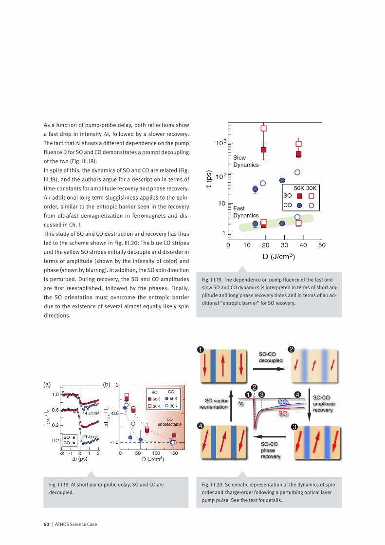
60 | ATHOS Science Case
Fig. III.20. Schematic representation of the dynamics of spin-order and charge-order following a perturbing optical laser pump pulse. See the text for details.
As a function of pump-probe delay, both reflections show a fast drop in intensity ΔI, followed by a slower recovery. The fact that ΔI shows a different dependence on the pump fluence D for SO and CO demonstrates a prompt decoupling of the two (Fig. III.18).In spite of this, the dynamics of SO and CO are related (Fig. III.19), and the authors argue for a description in terms of time-constants for amplitude recovery and phase recovery. An additional long-term sluggishness applies to the spin-order, similar to the entropic barrier seen in the recovery from ultrafast demagnetization in ferromagnets and dis-cussed in Ch. I.This study of SO and CO destruction and recovery has thus led to the scheme shown in Fig. III.20: The blue CO stripes and the yellow SO stripes initially decouple and disorder in terms of amplitude (shown by the intensity of color) and phase (shown by blurring). In addition, the SO spin direction is perturbed. During recovery, the SO and CO amplitudes are first reestablished, followed by the phases. Finally, the SO orientation must overcome the entropic barrier due to the existence of several almost equally likely spin directions.
Fig. III.18. At short pump-probe delay, SO and CO are decoupled.
Fig. III.19. The dependence on pump fluence of the fast and slow SO and CO dynamics is interpreted in terms of short am-plitude and long phase recovery times and in terms of an ad-ditional “entropic barrier” for SO recovery.

ATHOS Science Case | 61
Complexity in correlated electron materials
In a much cited paper, Dagotto [19] discusses the concept of complexity in connection with correlated electron materi-als. The essential point is that the competition between the charge-spin-orbital-lattice degrees of freedom can lead to the coexistence of different phases which are virtually de-generate in energy, and hence to inhomogeneities and glassy dynamics on a wide range of length and time scales.A hallmark of such “complex matter”, which exists “at the edge of chaos”, is a non-linear “giant” response to a small perturbation. For example, charge transport in manganite TMOs is different from that in simple metals: an isolated charge may strongly perturb its local environment, inducing the creation of a polaron, which may then attract other polarons to form larger, long-range structures. The mangan-ite phase diagram was shown in Figure III.4 a, with the close juxtaposition of ferromagnetic metal (FM) and antiferromag-
netic insulator (AFI) phases. The complexity view of the magnetic-field-induced metal-insulator transition in this material is that a ground state exists with quenched disorder, arising perhaps from lattice distortion accompanying chem-ical doping (see Fig. III.21 a), with a glassy intermixture of FM and AFI phases (see Fig. III.21 b). A small applied mag-netic field is then sufficient to tip the energy balance in favor of the FM phase, causing a giant, percolative change in the bulk conductivity.Also the cuprate superconductors show a variety of na-noscale inhomogenieties (see Fig. III.22), including the charge-spin stripes mentioned earlier (see Figs. III.5 b and III.16). Although the importance of stripes to the mechanism of high-temperature superconductivity is in question, also these materials appear to exhibit a giant response: A S–N–S (superconductor – normal conductor – superconductor) junction made of cuprate materials, whose N-layer thickness exceeds 100 coherence lengths, behaves as if it were a S-S
Fig. III.21. a) Lattice strain, e.g., arising from fluctuations in chemical doping, produces a slight local preference for a particular phase [20]. b) On a coarser scale, a small external perturbation, such as an applied magnetic field, can cause a non-linear, “giant” percolative change in the macroscopic conductivity [19].
a) b)
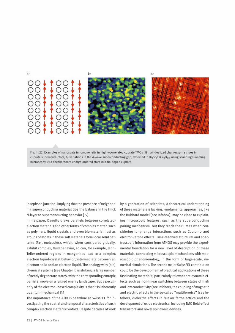
62 | ATHOS Science Case
Josephson junction, implying that the presence of neighbor-ing superconducting material tips the balance in the thick N-layer to superconducting behavior [19].In his paper, Dagotto draws parallels between correlated-electron materials and other forms of complex matter, such as polymers, liquid crystals and even bio-material. Just as groups of atoms in these soft materials form local solid pat-terns (i.e., molecules), which, when considered globally, exhibit complex, fluid behavior, so can, for example, Jahn-Teller-ordered regions in manganites lead to a complex electron liquid-crystal behavior, intermediate between an electron solid and an electron liquid. The analogy with (bio)chemical systems (see Chapter II) is striking: a large number of nearly degenerate states, with the corresponding entropic barriers, move on a rugged energy landscape. But a peculi-arity of the electron- based complexity is that it is inherently quantum-mechanical [19].The importance of the ATHOS beamline at SwissFEL for in-vestigating the spatial and temporal characteristics of such complex electron matter is twofold. Despite decades of work
by a generation of scientists, a theoretical understanding of these materials is lacking. Fundamental approaches, like the Hubbard model (see Infobox), may be close to explain-ing microscopic features, such as the superconducting pairing mechanism, but they reach their limits when con-sidering long-range interactions such as Coulomb and electron-lattice effects. Time-resolved structural and spec-troscopic information from ATHOS may provide the experi-mental foundation for a new level of description of these materials, connecting microscospic mechanisms with mac-roscopic phenomenology, in the form of large-scale, nu-merical simulations. The second major SwissFEL contribution could be the development of practical applications of these fascinating materials: particularly relevant are dynamic ef-fects such as non-linear switching between states of high and low conductivity (see Infobox), the coupling of magnetic and electric effects in the so-called “multiferroics” (see In-fobox), dielectric effects in relaxor ferroelectrics and the development of oxide electronics, including TMO field-effect transistors and novel spintronic devices.
Fig. III.22. Examples of nanoscale inhomogeneity in highly-correlated cuprate TMOs [19]. a) Idealized charge/spin stripes in cuprate superconductors, b) variations in the d-wave superconducting gap, detected in Bi2Sr2CaCu2O8+δ using scanning tunneling microscopy, c) a checkerboard charge-ordered state in a Na-doped cuprate.
a) b) c)
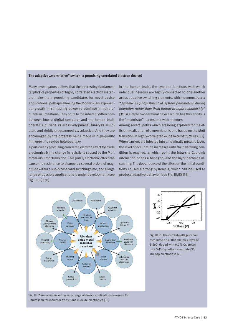
ATHOS Science Case | 63
The adaptive „memristive“ switch: a promising correlated electron device?
Many investigators believe that the interesting fundamen-tal physics properties of highly correlated electron materi-als make them promising candidates for novel device applications, perhaps allowing the Moore’s law exponen-tial growth in computing power to continue in spite of quantum limitations. They point to the inherent differences between how a digital computer and the human brain operate: e.g., serial vs. massively parallel, binary vs. multi-state and rigidly programmed vs. adaptive. And they are encouraged by the progress being made in high-quality film growth by oxide heteroepitaxy.A particularly promising correlated electron effect for oxide electronics is the change in resistivity caused by the Mott metal-insulator transition: This purely electronic effect can cause the resistance to change by several orders of mag-nitude within a sub-picosecond switching time, and a large range of possible applications is under development (see Fig. III.i7) [30].
In the human brain, the synaptic junctions with which individual neurons are highly connected to one another act as adaptive switching elements, which demonstrate a “dynamic self-adjustment of system parameters during operation rather than fixed output-to-input relationship” [31]. A simple two-terminal device which has this ability is the “memristor” – a resistor with memory.Among several paths which are being explored for the ef-ficient realization of a memristor is one based on the Mott transition in highly-correlated oxide heterostructures [32]. When carriers are injected into a nominally metallic layer, the level of occupation increases until the half-filling con-dition is reached, at which point the intra-site Coulomb interaction opens a bandgap, and the layer becomes in-sulating. The dependence of the effect on the initial condi-tions causes a strong hysteresis, which can be used to produce adaptive behavior (see Fig. III.i8) [33].
Fig. III.i8. The current-voltage curve measured on a 300 nm thick layer of SrZrO3 doped with 0.2% Cr, grown on a SrRuO3 bottom electrode [33]. The top electrode is Au.
Fig. III.i7. An overview of the wide range of device applications foreseen for ultrafast metal-insulator transitions in oxide electronics [30].
64 | ATHOS Science Case
Summary
• The charge, spin, orbital and lattice degrees of freedom of correlated electron materials lead to the inhomogene-ous and dynamic coexistence of material phases with novel orderings. Prominent examples, the dynamic polarons in manganites and the charge-spin stripes in cuprates and nickelates, have characteristic time and length scales (ps and nm) which are well-suited to be studied with the ATHOS beamline at SwissFEL.
• X-ray diffraction and the resonant X-ray techniques of elastic diffraction and inelastic scattering provide high sensitivity to charge, spin, orbital and lattice degrees of freedom, in wavelength ranges covered by the ATHOS beamline at SwissFEL. Furthermore, ATHOS will provide excellent access to the sub-ps dynamics of these degrees of freedom, either using laser-pump/X-ray probe experiments or by sampling equilibrium fluctuations via the intermediate scattering function S(Q,t).
• Photoemission spectroscopy, a preferred technique for static studies of correlated electron materials in the laboratory and at synchrotrons, is poorly suited to time-resolved measurements at the SwissFEL, due to resolution degradation by electron space-charge effects. However, the sensitivity to electronic structure provided by the photon-in/photon-out X-ray absorption and resonant scattering techniques make them highly promising alternatives, particularly in single-shot mode.
• The nature of metal-insulator transitions in correlated-electron materials can be elegantly determined by time-resolved pump-probe experiments. In this way, the metal-insulator transition in 1T-TaS2 is shown, by its ultrafast character (i.e., much faster than typical lattice vibratons), to be due to the electronic Mott-Hubbard transition, and not to the lattice-related Peierls instability.
• The electron-phonon interaction can be directly studied in time-resolved pump-probe experiments. An example is the triggering of a dynamic metal-insulator transition by the IR-excitation of a particular phonon mode in Pr0.7Ca0.3MnO3. With a further IR-pump/X-ray experiment, the dynamics of stripe order in La1.75Sr0.25NiO4 has been elucidated.
• In many respects, correlated-electron materials exhibit electronic complexity, characterized by glassy dynamics and giant responses to small external perturbations. This complexity is reminiscent of that of molecular systems, such as liquid crystals and even biological macromolecules. The ability of the ATHOS beamline at SwissFEL to provide novel information over a large range of time and length scales makes it an ideal tool to establish an experimental foundation for a unification in the theory of correlated electrons at the micro- and macro-scales.

ATHOS Science Case | 65
References
[1] Johnson, S., (private communication)[2] Bednorz, J. G. & Muller, K. A., “Possible High-Tc
Superconductivity in the Ba-La-Cu-O System,” Zeitschrift Fur Physik B-Condensed Matter 64, 189-193 (1986).
[3] Castleton, C. W. M. & Altarelli, M., “Orbital ordering in the manganites: Resonant x-ray scattering predictions at the manganese L-II and L-III edges,” Physical Review B 62, 1033-1038 (2000).
[4] Lynn, J. W., Argyriou, D. N., Ren, Y., Chen, Y., Mukovskii, Y. M. & Shulyatev, D. A., “Order and dynamics of intrinsic nanoscale inhomogeneities in manganites,” Physical Review B 76, 01443-7 (2007).
[5] Kivelson, S. A., Bindloss, I. P., Fradkin, E., Oganesyan, V., Tranquada, J. M., Kapitulnik, A. & Howald, C., “How to detect fluctuating stripes in the high-temperature superconductors,” Reviews of Modern Physics 75, 1201-1241 (2003).
[6] Als-Nielsen, J. & McMorrow, D., Elements of Modern X-Ray Physics (ed. Wiley) (2001).
[7] Altarelli, M., “Resonant x-ray scattering: A theoretical introduction”, Lect. Notes Phys. 697, 201-242 (2004).
[8] Lorenzo, J. E. (private communication)[9] Joly, Y. (private communication)[10] Ren, Y. H., Hu, Y. F., Li, Q., Hong, C. S., Hur, N. H. & Lupke, G.
“Ultrafast collective dynamics of short-range charge/orbital ordering fluctuations in colossal magnetoresistive oxides”, cond-mat/0310360v1 (2003).
[11] Schmitt, Th. (private communication)[12] Grubel, G., Stephenson, G. B., Gutt, C., Sinn, H. &
Tschentscher, T., “XPCS at the European X-ray free electron laser facility,” Nuclear Instruments & Methods in Physics Research Section B-Beam Interactions with Materials and Atoms 262, 357-367 (2007).
[13] Goodman, J. W., Statistical Optics (Wiley Classics Library, 2000).
[14] Peierls, R. E., Quantum Theory of Solids (Oxford University Press, 2004).
[15] Wolf, M. (private communication)[16] Perfetti, L., Loukakos, P. A., Lisowski, M., Bovensiepen, U.,
Wolf, M., Berger, H., Biermann, S. & Georges, A., “Femtosecond dynamics of electronic states in the Mott insulator 1T-TaS2 by time resolved photoelectron spectroscopy,” New Journal of Physics 10, 053019 (2008).
[17] Rini, M., Tobey, R., Dean, N., Itatani, J., Tomioka, Y., Tokura, Y., Schoenlein, R. W. & Cavalleri, A., “Control of the electronic phase of a manganite by mode-selective vibrational excitation,” Nature 449, 72-74 (2007).
[18] Cavalleri, A., (private communication)
[19] Dagotto, E., “Complexity in strongly correlated electronic systems,” Science 309, 257-262 (2005).
[20] Milhaly, L. http://solidstate.physics.sunysb.edu/talk/2004_dubrovnik2/.
[21] Cheong, S-W. & Mostovoy, M., “Multiferroics: a magnetic twist for ferroelectricity”, Nature Materials, 6, 13-20 (2007).
[22] Strocov, V.N., “Concept of a spectrometer for resonant inelastic X-ray scattering with parallel detection in incoming and outgoing photon energies”, J. Synch. Rad. 17, 1 (2010).
[23] Abbamonte, P., (private communication)[24] Sekikawa, T., Kosuge, A., Kanai, T. & Watanabe, S.,
“Nonlinear optics in the extreme ultraviolet,” Nature 432, 605-608 (2004).
[25] Gutt, C., (private communication)[26] Gutt, C., Stadler, L. M., Duri, A., Autenrieth, T., Leupold, O.,
Chushkin, Y. & Grubel, G., “Measuring temporal speckle correlations at ultrafast x-ray sources,” Optics Express 17, 55-61 (2009).
[27] Hubbard, J., “Electron Correlations in Narrow Energy Bands,” Proceedings of the Royal Society of London Series a-Mathematical and Physical Sciences 276, 238 (1963).
[28] Scalettar, R. T., “Elementary Introduction to the Hubbard Model,” http://leopard.physics.vcdavis.edu/rts/p210/hubbard7.pdf.
[29] Chuang, Y.C., et al, “Real-Time Manifestation of Strongly Coupled Spin and Charge Order Parameters in Stripe-Ordered La1.75Sr0.25NiO4 Nickelate Crystals Using Time-Resolved Resonant X-Ray Diffraction”, Phys. Rev. Lett. 110, 127404 (2013).
[30] Yang, Z., Ko, C. and Ramanathan, S., “Oxide electronics utilizing ultrafast metal-insulator transitions”, Annu. Rev. Mater. Res. 41, 337-67 (2011).
[31] Ha, S.D. and Ramanathan, S., “Adaptive oxide electronics: a review”, J. Appl. Phys. 110, 071101 (2011).
[32] Rozenberg, M.J., Inoue, I.H. and Sanchez, M.J., “Strong electron correlation effects in nonvolatile electronic memory devices”, Appl. Phys. Lett. 88, 033510 (2006).
[33] Beck, A., Bednorz, J.G., Gerber, Ch., Rossel, C. and Widmer, D., “Reproducible switching effect in thin oxide films for memory applications”, Appl. Phys. Lett. 77, 139 (2000).

66 | ATHOS Science Case
The first optical laser emitted light in 1960, producing high-intensity coherent radiation. This opened the now vast field of non-linear optics, including effects such as sum and difference frequency generation, self-focusing, solitons and stimulated Raman scattering. Some fifty-five years later, the X-ray free electron laser has the potential of extending these effects to the soft X-ray regime. An important possible advantage of such an extension would be the ability, by using the stimulated excitation of element-specific core levels, to excite and probe matter in a highly efficient manner at pre-determined atomic sites.
IV. Non-linear X-ray scienceThe invention 50 years ago of the optical laser opened the important field of non-linear optics: Will the ATHOS beamline at SwissFEL do the same at soft X-ray wavelengths?
• Resonant Inelastic X-ray Scattering
• Linear and non-linear optics
• Stimulated X-ray Raman scattering
• Experimental methods

ATHOS Science Case | 67
Resonant inelastic X-ray scattering
As described in Chapter III, resonant inelastic X-ray scatter-ing (RIXS) is a synchrotron-based, photon-in photon-out, chemically-specific spectroscopic method which allows the study of collective valence electron excitations in solids (Ω = 0.05 – 5 eV), without the limitations of probing depth, low ambient EM-fields, sample conductivity and surface quality presented by photoemission. In spite of resonance enhancement, the main drawback of RIXS is its low effi-ciency, generally 10-5 of elastic Rayleigh scattering, implying that a typical spectral measurement requires hours at a third generation undulator beamline. This low efficiency limits the possibility at a synchrotron of time-dependent, pump-probe RIXS measurements.Like its Raman scattering optical analog, the RIXS technique relies on spontaneous emission from a photo-excited state to produce the observed outgoing photon. At sufficiently high incoming photon fluence, the efficiency of stimulated Raman scattering exceeds that of the spontaneous process, with gains in efficiency at optical wavelengths of up to 107. And using ps and fs optical pulses, a variety of techniques have been devised of performing time-dependent stimulated Raman scattering, some of which make explicit use of the
large bandwidth of the exciting radiation, and some of which require several pulses, often with different wavelengths.With the advent at XFELs of fs X-ray pulses with extreme peak brightness, and perhaps in the near future of multi-pulse and multi-color capabilities, it is interesting to consider the feasibility of time-resolved, non-linear X-ray spectroscopy [1]. This Chapter begins by making the distinction between spontaneous and stimulated RIXS and highlighting the importance of the third-order susceptibility χ(3) in these and related processes. Using a simple quantum mechanical model and information on the transition dipole moment obtained from excited state lifetimes, an estimation is made of χ(3) at X-ray wavelengths, which can then be used to compute cross-sections for stimulated scattering. It then becomes clear that stimulated X-ray Raman scattering is best observed at soft X-ray wavelengths (ω = 0.5 – 1.5 keV). In order to avoid the necessity of simultaneous irradiation with two different wavelengths, a broadband impulsive method is described where a single pulse delivers both of the frequency components required for stimulated scatter-ing. This then leads to a discussion of double-pulse X-ray pump / X-ray probe measurements of excitation dynamics, analogous to the time-resolved coherent anti-Stokes Raman scattering (CARS) technique.
Figure IV.1. Schematic representations of selected light-matter interactions [1]. See the text for explanations.

68 | ATHOS Science Case
Simulating SASE pulses
To aid in the design of XFEL sources and experiments, it is often necessary to consider the interaction of simulated SASE (self-amplifying spontaneous emission) pulses with matter. This is particularly true for non-linear X-ray optics. There exist sophisticated codes which predict the emission characteristics of an XFEL from first principles [14], but when a statistical analysis is necessary, they are generally too slow to deliver the required large number of simulated pulses.A fast, simple approximative method of simulating SASE pulses has been given by Pfeifer [15]. Besides the average central wavelength and pulse energy, it requires three input parameters, the average rms pulse bandwidth σω, the average rms pulse duration σt (also equal to the inverse of the spectral width of a typical SASE frequency spike), and a frequency bin width δω (see Fig. IV.i.1).For a simulation of soft X-ray SASE pulses at the L3 edge of Cu, we take: ω0 = 933 eV, σω = 2.5 eV, σt = 1.8 fs and δω = 0.2 eV. The procedure goes as follows (see Fig. IV.i.2.):A: Start with a Gaussian frequency distribution centered
on ω0 and with rms width σω.B: Multiply each frequency point by a random phasor eiφω.C: Fourier transform to the time-domain, yielding a noisy
pulse of infinite duration.
D: Generate a Gaussian time filter with rms width σt.E: Multiply the time pulse C with the time filter, yielding a
finite pulse.F: The absolute amplitude squared gives the time pulse
intensity.G: An inverse Fourier transform of the time pulse E gives
the amplitude spectrum.H: The absolute amplitude squared gives the spectral pulse
intensity.
Fig. IV.i1. A schematic SASE pulse, showing the input parame-ters required for Pfeifer’s [15] simulation code.
Fig. IV.i2. Steps in the Pfeifer’s [15] simulation of a SASE pulse. See text for details.

ATHOS Science Case | 69
Linear and non-linear optics
Selected light-matter interactionsThe direct photo-excitation of a low-lying transition, loosely denoted IR-absorption, is possible in a sample if the electric dipole operator μ joins the ground state g and a low-level excited state f (Fig. IV.1a). With short wavelength radiation ω1, one can resonantly excite a higher-lying state e and observe the subsequent radiative decay ω2 (fluorescence) to the state f (Fig. IV.1b). Using X-rays to excite, the intermediate state is a short-lived (5-10 fs) core-hole, and the principal competitor to fluores-cence decay is the emission of an Auger electron. A small fraction of the optical photons incident on a sample may undergo inelastic, Raman scattering (Fig. IV.1c). Provided the electric polarizability α joins the states g and f, this effectively instantaneous single-step process emits the outgoing inelastic Stokes photon ω2. Raman scattering is described in terms of the third-order susceptibility χ(3) or via the Kramers-Heisenberg formalism (see Ch. III). For the cases IV.1b-1c, a spectral measurement of the outgoing radiation yields the low-lying excitation energy Ω = ω1– ω2.Enhanced efficiency results when the incoming ω1 photon is resonant with a true excited state transition g→e (Fig. IV.1d). In the optical regime, this is termed resonance Raman scattering, the optical analog of resonant inelastic X-ray scattering (RIXS). Finally, if besides ω1, a sufficiently large fluence of incident ω2 photons is present, stimulated, rather than spontaneous, decay of the intermediate state e pre-dominates, coherently amplifying the wavefield ω2 via Raman gain (Fig. IV.1e) [2]. Note that there is no threshold for stimulated Raman scattering.
Non-linear optics considerationsSpontaneous and stimulated Raman scattering are examples of non-linear optical spectroscopies, and these are divided into two categories:a) A parametric (p) process, also called passive or elastic,
leaves the material properties unchanged, if one disre-gards a small energy dissipation in the intermediate state.
b) In a non-parametric (np) process, also called active or inelastic, the material undergoes a large energy loss to or gain from the radiation field.
The interaction of a polarizable material with a varying electric field produces a time-dependent electric polariza-tion, which can be expanded as a power series in the field strength:
P t( ) = ε0 χ 1( )E t( ) + χ 2( )E2 t( ) + χ 3( )E 3 t( ) + ...⎡⎣ ⎤⎦
≡ P 1( ) t( ) + P 2( ) t( ) + P 3( ) t( ) + ...
P s( ) ω k( ) = ε0χ
s( ) ω k =ω1 +ω2 + ... +ω s( )E ω1( ) ... E ω s( )
For a superposition of light waves, where the electric field consists of several oscillating components, the non-linear terms in the polarization mix contributions with different frequencies, and the resulting Fourier components of the polarization are expressed in terms of the frequency-depend-ent non-linear susceptibilities χ(s):
P t( ) = ε0 χ 1( )E t( ) + χ 2( )E2 t( ) + χ 3( )E 3 t( ) + ...⎡⎣ ⎤⎦
≡ P 1( ) t( ) + P 2( ) t( ) + P 3( ) t( ) + ...
P s( ) ω k( ) = ε0χ
s( ) ω k =ω1 +ω2 + ... +ω s( )E ω1( ) ... E ω s( )
where the frequency ωk can be any algebraic sum of the (positive and negative) frequencies which are active in the interaction.The source term for parametric processes of any order is proportional to the corresponding susceptibility, and the cross-section for a non-parametric process is proportional to the imaginary part of an odd-order susceptibility times the modulus squared of each field involved. Non-paramet-ric interactions thus require the presence of a nearby reso-nance. Materials with inversion symmetry have a vanishing second-order susceptibility. Examples of light-matter inter-actions are:a) 1st order np: single-photon absorption or emissionb) 1st order p: light propagation with linear dispersionc) 2nd order p: second-harmonic generationd) 3rd order np: spontaneous and stimulated Raman scat-
tering, governed by χ(3) (ω2 = ω2 + ω1 – ω1)e) 3rd order p: four-wave mixing, and in particular, coherent
anti-Stokes Raman scattering (CARS), governed by χ(3) (ωs = ω1 – ω2 + ω1)
Stimulated X-ray Raman Scattering
Quantum mechanical calculation of χ(3) Following the book of Boyd [3], we perform a quantum-mechanical calculation of the third-order susceptibility. We
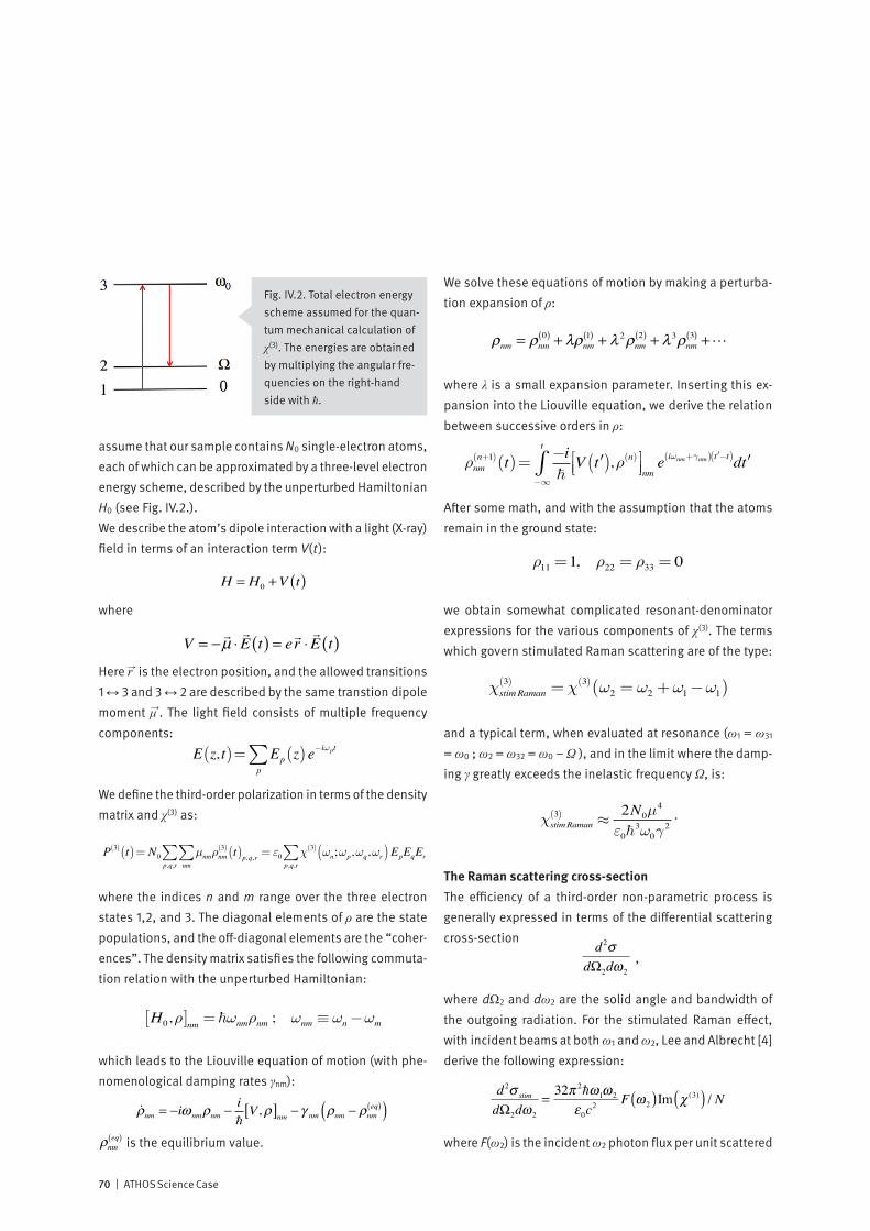
70 | ATHOS Science Case
assume that our sample contains N0 single-electron atoms, each of which can be approximated by a three-level electron energy scheme, described by the unperturbed Hamiltonian H0 (see Fig. IV.2.).We describe the atom’s dipole interaction with a light (X-ray) field in terms of an interaction term V(t):
H = H0 +V t( )
V = −µ ⋅E t( ) = e r ⋅
E t( )
where
H = H0 +V t( )
V = −µ ⋅E t( ) = e r ⋅
E t( )
Here r→ is the electron position, and the allowed transitions 1 ↔ 3 and 3 ↔ 2 are described by the same transtion dipole moment μ→. The light field consists of multiple frequency components:
E z, t( )= Ep z( )p∑ e−iωpt
P 3( ) t( )= N0 µnmρnm3( )
nm∑ t( )p,q, r
p,q,r∑ = ε0 χ 3( )
p,q,r∑ ωn;ωp,ωq,ωr( )EpEqEr
H0,ρ[ ]nm =ωnmρnm ; ωnm ≡ωn−ωm
ρnm = −iωnmρnm −iV,ρ[ ]nm −γ nm ρnm − ρnm
eq( )( )
ρnm = ρnm0( ) + λρnm
1( ) + λ 2ρnm2( ) + λ 3ρnm
3( ) +
ρnmn+1( ) t( )= −i
−∞
t
∫ V ′t( ),ρ n( )⎡⎣⎢
⎤⎦⎥nm e
iωnm+γnm( ) ′t −t( )d ′t
ρ11=1, ρ22 = ρ33 = 0
We define the third-order polarization in terms of the density matrix and χ(3) as:
E z, t( )= Ep z( )p∑ e−iωpt
P 3( ) t( )= N0 µnmρnm3( )
nm∑ t( )p,q, r
p,q,r∑ = ε0 χ 3( )
p,q,r∑ ωn;ωp,ωq,ωr( )EpEqEr
H0,ρ[ ]nm =ωnmρnm ; ωnm ≡ωn−ωm
ρnm = −iωnmρnm −iV,ρ[ ]nm −γ nm ρnm − ρnm
eq( )( )
ρnm = ρnm0( ) + λρnm
1( ) + λ 2ρnm2( ) + λ 3ρnm
3( ) +
ρnmn+1( ) t( )= −i
−∞
t
∫ V ′t( ),ρ n( )⎡⎣⎢
⎤⎦⎥nm e
iωnm+γnm( ) ′t −t( )d ′t
ρ11=1, ρ22 = ρ33 = 0
where the indices n and m range over the three electron states 1,2, and 3. The diagonal elements of ρ are the state populations, and the off-diagonal elements are the “coher-ences”. The density matrix satisfies the following commuta-tion relation with the unperturbed Hamiltonian:
E z, t( )= Ep z( )p∑ e−iωpt
P 3( ) t( )= N0 µnmρnm3( )
nm∑ t( )p,q, r
p,q,r∑ = ε0 χ 3( )
p,q,r∑ ωn;ωp,ωq,ωr( )EpEqEr
H0,ρ[ ]nm =ωnmρnm ; ωnm ≡ωn−ωm
ρnm = −iωnmρnm −iV,ρ[ ]nm −γ nm ρnm − ρnm
eq( )( )
ρnm = ρnm0( ) + λρnm
1( ) + λ 2ρnm2( ) + λ 3ρnm
3( ) +
ρnmn+1( ) t( )= −i
−∞
t
∫ V ′t( ),ρ n( )⎡⎣⎢
⎤⎦⎥nm e
iωnm+γnm( ) ′t −t( )d ′t
ρ11=1, ρ22 = ρ33 = 0
which leads to the Liouville equation of motion (with phe-nomenological damping rates γnm):
E z, t( )= Ep z( )p∑ e−iωpt
P 3( ) t( )= N0 µnmρnm3( )
nm∑ t( )p,q, r
p,q,r∑ = ε0 χ 3( )
p,q,r∑ ωn;ωp,ωq,ωr( )EpEqEr
H0,ρ[ ]nm =ωnmρnm ; ωnm ≡ωn−ωm
ρnm = −iωnmρnm −iV,ρ[ ]nm −γ nm ρnm − ρnm
eq( )( )
ρnm = ρnm0( ) + λρnm
1( ) + λ 2ρnm2( ) + λ 3ρnm
3( ) +
ρnmn+1( ) t( )= −i
−∞
t
∫ V ′t( ),ρ n( )⎡⎣⎢
⎤⎦⎥nm e
iωnm+γnm( ) ′t −t( )d ′t
ρ11=1, ρ22 = ρ33 = 0
is the equilibrium value.
We solve these equations of motion by making a perturba-tion expansion of ρ:
E z, t( )= Ep z( )p∑ e−iωpt
P 3( ) t( )= N0 µnmρnm3( )
nm∑ t( )p,q, r
p,q,r∑ = ε0 χ 3( )
p,q,r∑ ωn;ωp,ωq,ωr( )EpEqEr
H0,ρ[ ]nm =ωnmρnm ; ωnm ≡ωn−ωm
ρnm = −iωnmρnm −iV,ρ[ ]nm −γ nm ρnm − ρnm
eq( )( )
ρnm = ρnm0( ) + λρnm
1( ) + λ 2ρnm2( ) + λ 3ρnm
3( ) +
ρnmn+1( ) t( )= −i
−∞
t
∫ V ′t( ),ρ n( )⎡⎣⎢
⎤⎦⎥nm e
iωnm+γnm( ) ′t −t( )d ′t
ρ11=1, ρ22 = ρ33 = 0
where λ is a small expansion parameter. Inserting this ex-pansion into the Liouville equation, we derive the relation between successive orders in ρ:
E z, t( )= Ep z( )p∑ e−iωpt
P 3( ) t( )= N0 µnmρnm3( )
nm∑ t( )p,q, r
p,q,r∑ = ε0 χ 3( )
p,q,r∑ ωn;ωp,ωq,ωr( )EpEqEr
H0,ρ[ ]nm =ωnmρnm ; ωnm ≡ωn−ωm
ρnm = −iωnmρnm −iV,ρ[ ]nm −γ nm ρnm − ρnm
eq( )( )
ρnm = ρnm0( ) + λρnm
1( ) + λ 2ρnm2( ) + λ 3ρnm
3( ) +
ρnmn+1( ) t( )= −i
−∞
t
∫ V ′t( ),ρ n( )⎡⎣⎢
⎤⎦⎥nm e
iωnm+γnm( ) ′t −t( )d ′t
ρ11=1, ρ22 = ρ33 = 0
After some math, and with the assumption that the atoms remain in the ground state:
E z, t( )= Ep z( )p∑ e−iωpt
P 3( ) t( )= N0 µnmρnm3( )
nm∑ t( )p,q, r
p,q,r∑ = ε0 χ 3( )
p,q,r∑ ωn;ωp,ωq,ωr( )EpEqEr
H0,ρ[ ]nm =ωnmρnm ; ωnm ≡ωn−ωm
ρnm = −iωnmρnm −iV,ρ[ ]nm −γ nm ρnm − ρnm
eq( )( )
ρnm = ρnm0( ) + λρnm
1( ) + λ 2ρnm2( ) + λ 3ρnm
3( ) +
ρnmn+1( ) t( )= −i
−∞
t
∫ V ′t( ),ρ n( )⎡⎣⎢
⎤⎦⎥nm e
iωnm+γnm( ) ′t −t( )d ′t
ρ11=1, ρ22 = ρ33 = 0
we obtain somewhat complicated resonant-denominator expressions for the various components of χ(3). The terms which govern stimulated Raman scattering are of the type:
d 2σdΩ2dω2
d 2σ stim
dΩ2dω2
=32π 2ω1ω2
ε0c2 F ω2( )Im χ (3)( ) / N
FBB ω ,T( )∝ ω 2
c21
exp ω / kT( ) −1 +12
⎛⎝⎜
⎞⎠⎟
Fspon ω2( ) = FBB ω2 ,0( )∝ ω22
c2
χstimRaman3( ) =χ 3( ) ω2 =ω2+ω1−ω1( )
χstimRaman3( ) ≈
2N0µ4
ε03ω0γ
2
and a typical term, when evaluated at resonance (ω1 = ω31 = ω0 ; ω2 = ω32 = ω0 – Ω ), and in the limit where the damp-ing γ greatly exceeds the inelastic frequency Ω, is:
d 2σdΩ2dω2
d 2σ stim
dΩ2dω2
=32π 2ω1ω2
ε0c2 F ω2( )Im χ (3)( ) / N
FBB ω ,T( )∝ ω 2
c21
exp ω / kT( ) −1 +12
⎛⎝⎜
⎞⎠⎟
Fspon ω2( ) = FBB ω2 ,0( )∝ ω22
c2
χstimRaman3( ) =χ 3( ) ω2 =ω2+ω1−ω1( )
χstimRaman3( ) ≈
2N0µ4
ε03ω0γ
2.
The Raman scattering cross-sectionThe efficiency of a third-order non-parametric process is generally expressed in terms of the differential scattering cross-section
d 2σdΩ2dω2
d 2σ stim
dΩ2dω2
=32π 2ω1ω2
ε0c2 F ω2( )Im χ (3)( ) / N
FBB ω ,T( )∝ ω 2
c21
exp ω / kT( ) −1 +12
⎛⎝⎜
⎞⎠⎟
Fspon ω2( ) = FBB ω2 ,0( )∝ ω22
c2
χstimRaman3( ) =χ 3( ) ω2 =ω2+ω1−ω1( )
χstimRaman3( ) ≈
2N0µ4
ε03ω0γ
2
,
where dΩ2 and dω2 are the solid angle and bandwidth of the outgoing radiation. For the stimulated Raman effect, with incident beams at both ω1 and ω2, Lee and Albrecht [4] derive the following expression:
d 2σdΩ2dω2
d 2σ stim
dΩ2dω2
=32π 2ω1ω2
ε0c2 F ω2( )Im χ (3)( ) / N
FBB ω ,T( )∝ ω 2
c21
exp ω / kT( ) −1 +12
⎛⎝⎜
⎞⎠⎟
Fspon ω2( ) = FBB ω2 ,0( )∝ ω22
c2
χstimRaman3( ) =χ 3( ) ω2 =ω2+ω1−ω1( )
χstimRaman3( ) ≈
2N0µ4
ε03ω0γ
2
where F(ω2) is the incident ω2 photon flux per unit scattered
Fig. IV.2. Total electron energy scheme assumed for the quan-tum mechanical calculation of χ(3). The energies are obtained by multiplying the angular fre-quencies on the right-hand side with .
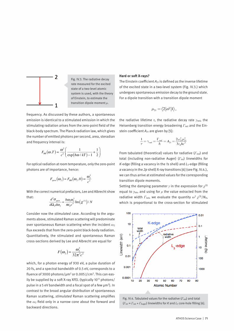
ATHOS Science Case | 71
frequency. As discussed by these authors, a spontaneous emission is identical to a stimulated emission in which the stimulating radiation arises from the zero-point field of the black-body spectrum. The Planck radiation law, which gives the number of emitted photons per second, area, steradian and frequency interval is:
d 2σdΩ2dω2
d 2σ stim
dΩ2dω2
=32π 2ω1ω2
ε0c2 F ω2( )Im χ (3)( ) / N
FBB ω ,T( )∝ ω 2
c21
exp ω / kT( ) −1 +12
⎛⎝⎜
⎞⎠⎟
Fspon ω2( ) = FBB ω2 ,0( )∝ ω22
c2
χstimRaman3( ) =χ 3( ) ω2 =ω2+ω1−ω1( )
χstimRaman3( ) ≈
2N0µ4
ε03ω0γ
2
For optical radiation at room temperature, only the zero-point photons are of importance, hence:
d 2σdΩ2dω2
d 2σ stim
dΩ2dω2
=32π 2ω1ω2
ε0c2 F ω2( )Im χ (3)( ) / N
FBB ω ,T( )∝ ω 2
c21
exp ω / kT( ) −1 +12
⎛⎝⎜
⎞⎠⎟
Fspon ω2( ) = FBB ω2 ,0( )∝ ω22
c2
χstimRaman3( ) =χ 3( ) ω2 =ω2+ω1−ω1( )
χstimRaman3( ) ≈
2N0µ4
ε03ω0γ
2
With the correct numerical prefactors, Lee and Albrecht show that:
d 2σ spon
dΩ2dω2
=ω1ω2
3
πε0c4 Im χ (3)( ) / N
F ω2( ) = ω22
32π 3c2
µ21= 2 er 1
Consider now the stimulated case. According to the argu-ments above, stimulated Raman scattering will predominate over spontaneous Raman scattering when the incident ω2 flux exceeds that from the zero-point black-body radiation. Quantitatively, the stimulated and spontaneous Raman cross-sections derived by Lee and Albrecht are equal for
d 2σ spon
dΩ2dω2
=ω1ω2
3
πε0c4 Im χ (3)( ) / N
F ω2( ) = ω22
32π 3c2
µ21= 2 er 1
which, for a photon energy of 930 eV, a pulse duration of 20 fs, and a spectral bandwidth of 0.5 eV, corresponds to a fluence of 3000 photons/μm2 or 0.005 J/cm2. This can eas-ily be supplied by a soft X-ray XFEL (typically 1013 photons/pulse in a 5 eV bandwidth and a focal spot of a few μm2). In contrast to the broad angular distribution of spontaneous Raman scattering, stimulated Raman scattering amplifies the ω2 field only in a narrow cone about the forward and backward directions.
Hard or soft X-rays?The Einstein coefficient A21 is defined as the inverse lifetime of the excited state in a two-level system (Fig. IV.3.) which undergoes spontaneous emission decay to the ground state. For a dipole transition with a transition dipole moment
d 2σ spon
dΩ2dω2
=ω1ω2
3
πε0c4 Im χ (3)( ) / N
F ω2( ) = ω22
32π 3c2
µ21= 2 er 1 ,
the radiative lifetime τ, the radiative decay rate γrad, the Heisenberg transition energy broadening Γrad and the Ein-stein coefficient A21 are given by [5]:
1τ= γrad =
Γrad= A21=
2ω213 µ21
2
3ε0hc3
From tabulated (theoretical) values for radiative (Γrad) and total (including non-radiative Auger) (Γtot) linewidths for K-edge (filling a vacancy in the 1s shell) and L3-edge (filling a vacancy in the 2p shell) X-ray transitions [6] (see Fig. IV.4.), we can thus arrive at estimated values for the corresponding transition dipole moments.Setting the damping parameter γ in the expression for χ(3) equal to γtot, and using for μ the value extracted from the radiative width Γrad, we evaluate the quantity ω2 χ(3)/N0, which is proportional to the cross-section for stimulated
Fig. IV.4. Tabulated values for the radiative (Γrad) and total (Γtot = Γrad + ΓAuger) linewidths for K and L3 core-hole filling [6].
Fig. IV.3. The radiative decay rate measured for the excited state of a two-level atomic system is used, with the theory of Einstein, to estimate the transition dipole moment μ.

72 | ATHOS Science Case
Raman scattering, for different atomic numbers Z and for the K and L3 edges (see Fig. IV.5.). We see that, in particular for the interesting 3d transition metal ions Z = 23-27, the soft X-ray L3 cross-section exceeds the hard X-ray K cross-section by approximately a factor 10. This is a strong argu-ment for preferring a soft X-ray XFEL to observe and investi-gate non-linear stimulated X-ray Raman scattering. Another reason for doing so is that L3-type transitions involve the partially-filled 3d shell (2p→3d) – just those electrons which are responsible for magnetism and electron correlation ef-fects in many solids.
Experimental methods
Impulsive stimulated Raman scatteringIt is clear from the schematic illustration of stimulated Ra-man scattering (Fig. IV.1e), that the simultaneous presence of two X-ray frequencies, ω1 and ω2, is required – something which is technologically difficult. But according to the fre-quency-time uncertainty principle, a Gaussian pulse of duration τFWHM will contain frequency components in a broad bandwidth ΔωFWHM, which is inversely proportional to the duration:
χ(3) for free electrons
At X-ray frequencies, it is tempting to assume that the majority of electrons in a solid can be treated as unbound. We thus evaluate the (classical) non-linear 3rd order sus-ceptibility for the case of free electrons. We allow an electron to interact with an electromagnetic wave, and we orient the electric and magnetic fields, which are related by
By =1cEx
x+γ x=−emEx +
emz By
z+γ z=−emx By
E t( )= E1 cosω1t+E2 cosω2t
P 3( ) = N0ex= ε0χ3( )E1
2E2
χ 3( ) ω2 =ω2+ω1−ω1( )= N0e4
8ε0m3c2
iγ ω2−2iγ( )ω12ω2
2 ω1+ω2( ) ω1−ω2+ iγ( )
along the x and the y axes, respectively. The (viscously-damped) equations of motion are then:
By =1cEx
x+γ x=−emEx +
emz By
z+γ z=−emx By
E t( )= E1 cosω1t+E2 cosω2t
P 3( ) = N0ex= ε0χ3( )E1
2E2
χ 3( ) ω2 =ω2+ω1−ω1( )= N0e4
8ε0m3c2
iγ ω2−2iγ( )ω12ω2
2 ω1+ω2( ) ω1−ω2+ iγ( )
By =1cEx
x+γ x=−emEx +
emz By
z+γ z=−emx By
E t( )= E1 cosω1t+E2 cosω2t
P 3( ) = N0ex= ε0χ3( )E1
2E2
χ 3( ) ω2 =ω2+ω1−ω1( )= N0e4
8ε0m3c2
iγ ω2−2iγ( )ω12ω2
2 ω1+ω2( ) ω1−ω2+ iγ( )
and the resulting electron path follows a “figure-eight” (Fig.IV.i3).
We now allow the electron to simultaneously interact with two co-progagating EM waves:
By =1cEx
x+γ x=−emEx +
emz By
z+γ z=−emx By
E t( )= E1 cosω1t+E2 cosω2t
P 3( ) = N0ex= ε0χ3( )E1
2E2
χ 3( ) ω2 =ω2+ω1−ω1( )= N0e4
8ε0m3c2
iγ ω2−2iγ( )ω12ω2
2 ω1+ω2( ) ω1−ω2+ iγ( )
and we define the non-linear polarization in terms of the dipole moment as:
By =1cEx
x+γ x=−emEx +
emz By
z+γ z=−emx By
E t( )= E1 cosω1t+E2 cosω2t
P 3( ) = N0ex= ε0χ3( )E1
2E2
χ 3( ) ω2 =ω2+ω1−ω1( )= N0e4
8ε0m3c2
iγ ω2−2iγ( )ω12ω2
2 ω1+ω2( ) ω1−ω2+ iγ( )
By iteratively solving the resulting equations of motion, and assuming a weak damping, it is straightforward, but tedious, to obtain the result:
By =1cEx
x+γ x=−emEx +
emz By
z+γ z=−emx By
E t( )= E1 cosω1t+E2 cosω2t
P 3( ) = N0ex= ε0χ3( )E1
2E2
χ 3( ) ω2 =ω2+ω1−ω1( )= N0e4
8ε0m3c2
iγ ω2−2iγ( )ω12ω2
2 ω1+ω2( ) ω1−ω2+ iγ( )
Evaluating this result, even under the assumption that all electrons participate, generally leads to a value which is many orders of magnitude less than that obtained at reso-nance from the quantum-mechanical atomic calculation. A similar calculation for the 2nd order susceptibility for free electrons also yields a non-zero result, in spite of the fact that χ(2) must vanish for problems with inversion symmetry. The explanation is that the Lorentz field of the EM wave breaks this symmetry, thus allowing, for example frequency-doubling to occur at X-ray wave lengths in in-version-symmetric materials.
Fig. IV.i3. The figure-eight path of an electron interacting with an electromagnetic wave.
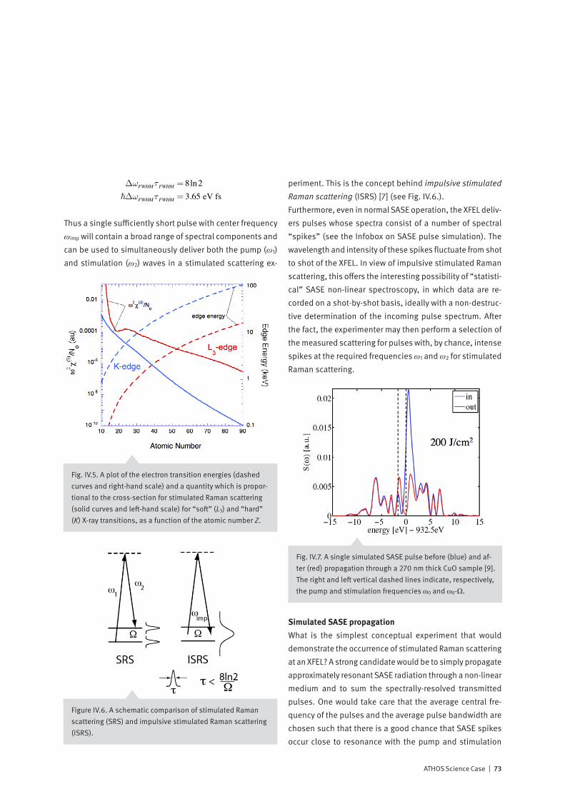
ATHOS Science Case | 73
ΔωFWHMτFWHM = 8ln2ΔωFWHMτFWHM = 3.65 eV fs
Thus a single sufficiently short pulse with center frequency ωimp will contain a broad range of spectral components and can be used to simultaneously deliver both the pump (ω1) and stimulation (ω2) waves in a stimulated scattering ex-
periment. This is the concept behind impulsive stimulated Raman scattering (ISRS) [7] (see Fig. IV.6.).Furthermore, even in normal SASE operation, the XFEL deliv-ers pulses whose spectra consist of a number of spectral “spikes” (see the Infobox on SASE pulse simulation). The wavelength and intensity of these spikes fluctuate from shot to shot of the XFEL. In view of impulsive stimulated Raman scattering, this offers the interesting possibility of “statisti-cal” SASE non-linear spectroscopy, in which data are re-corded on a shot-by-shot basis, ideally with a non-destruc-tive determination of the incoming pulse spectrum. After the fact, the experimenter may then perform a selection of the measured scattering for pulses with, by chance, intense spikes at the required frequencies ω1 and ω2 for stimulated Raman scattering.
Simulated SASE propagationWhat is the simplest conceptual experiment that would demonstrate the occurrence of stimulated Raman scattering at an XFEL? A strong candidate would be to simply propagate approximately resonant SASE radiation through a non-linear medium and to sum the spectrally-resolved transmitted pulses. One would take care that the average central fre-quency of the pulses and the average pulse bandwidth are chosen such that there is a good chance that SASE spikes occur close to resonance with the pump and stimulation
Figure IV.6. A schematic comparison of stimulated Raman scattering (SRS) and impulsive stimulated Raman scattering (ISRS).
Fig. IV.7. A single simulated SASE pulse before (blue) and af-ter (red) propagation through a 270 nm thick CuO sample [9]. The right and left vertical dashed lines indicate, respectively, the pump and stimulation frequencies ω0 and ω0-Ω.
Fig. IV.5. A plot of the electron transition energies (dashed curves and right-hand scale) and a quantity which is propor-tional to the cross-section for stimulated Raman scattering (solid curves and left-hand scale) for “soft” (L3) and “hard” (K) X-ray transitions, as a function of the atomic number Z.
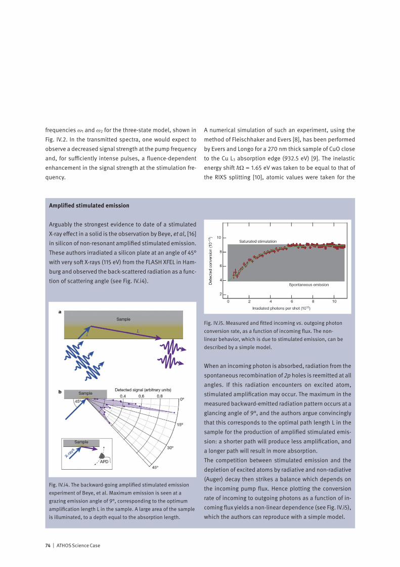
74 | ATHOS Science Case
frequencies ω1 and ω2 for the three-state model, shown in Fig. IV.2. In the transmitted spectra, one would expect to observe a decreased signal strength at the pump frequency and, for sufficiently intense pulses, a fluence-dependent enhancement in the signal strength at the stimulation fre-quency.
A numerical simulation of such an experiment, using the method of Fleischhaker and Evers [8], has been performed by Evers and Longo for a 270 nm thick sample of CuO close to the Cu L3 absorption edge (932.5 eV) [9]. The inelastic energy shift Ω = 1.65 eV was taken to be equal to that of the RIXS splitting [10], atomic values were taken for the
Amplified stimulated emission
Arguably the strongest evidence to date of a stimulated X-ray effect in a solid is the observation by Beye, et al, [16] in silicon of non-resonant amplified stimulated emission. These authors irradiated a silicon plate at an angle of 45° with very soft X-rays (115 eV) from the FLASH XFEL in Ham-burg and observed the back-scattered radiation as a func-tion of scattering angle (see Fig. IV.i4).
When an incoming photon is absorbed, radiation from the spontaneous recombination of 2p holes is reemitted at all angles. If this radiation encounters on excited atom, stimulated amplification may occur. The maximum in the measured backward-emitted radiation pattern occurs at a glancing angle of 9°, and the authors argue convincingly that this corresponds to the optimal path length L in the sample for the production of amplified stimulated emis-sion: a shorter path will produce less amplification, and a longer path will result in more absorption.The competition between stimulated emission and the depletion of excited atoms by radiative and non-radiative (Auger) decay then strikes a balance which depends on the incoming pump flux. Hence plotting the conversion rate of incoming to outgoing photons as a function of in-coming flux yields a non-linear dependence (see Fig. IV.i5), which the authors can reproduce with a simple model.
Fig. IV.i4. The backward-going amplified stimulated emission experiment of Beye, et al. Maximum emission is seen at a grazing emission angle of 9°, corresponding to the optimum amplification length L in the sample. A large area of the sample is illuminated, to a depth equal to the absorption length.
Fig. IV.i5. Measured and fitted incoming vs. outgoing photon conversion rate, as a function of incoming flux. The non- linear behavior, which is due to stimulated emission, can be described by a simple model.
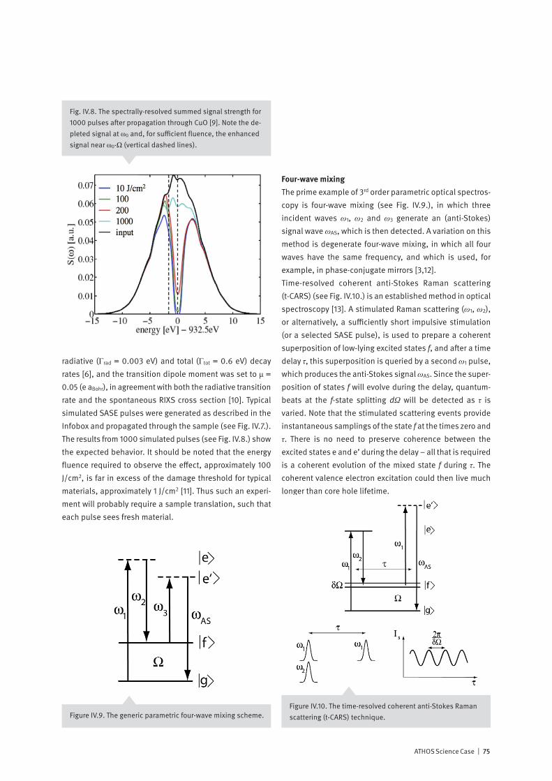
ATHOS Science Case | 75
radiative (Γrad = 0.003 eV) and total (Γtot = 0.6 eV) decay rates [6], and the transition dipole moment was set to μ = 0.05 (e aBohr), in agreement with both the radiative transition rate and the spontaneous RIXS cross section [10]. Typical simulated SASE pulses were generated as described in the Infobox and propagated through the sample (see Fig. IV.7.). The results from 1000 simulated pulses (see Fig. IV.8.) show the expected behavior. It should be noted that the energy fluence required to observe the effect, approximately 100 J/cm2, is far in excess of the damage threshold for typical materials, approximately 1 J/cm2 [11]. Thus such an experi-ment will probably require a sample translation, such that each pulse sees fresh material.
Four-wave mixingThe prime example of 3rd order parametric optical spectros-copy is four-wave mixing (see Fig. IV.9.), in which three incident waves ω1, ω2 and ω3 generate an (anti-Stokes) signal wave ωAS, which is then detected. A variation on this method is degenerate four-wave mixing, in which all four waves have the same frequency, and which is used, for example, in phase-conjugate mirrors [3,12].Time-resolved coherent anti-Stokes Raman scattering (t-CARS) (see Fig. IV.10.) is an established method in optical spectroscopy [13]. A stimulated Raman scattering (ω1, ω2), or alternatively, a sufficiently short impulsive stimulation (or a selected SASE pulse), is used to prepare a coherent superposition of low-lying excited states f, and after a time delay τ, this superposition is queried by a second ω1 pulse, which produces the anti-Stokes signal ωAS. Since the super-position of states f will evolve during the delay, quantum-beats at the f-state splitting dΩ will be detected as τ is varied. Note that the stimulated scattering events provide instantaneous samplings of the state f at the times zero and τ. There is no need to preserve coherence between the excited states e and e’ during the delay – all that is required is a coherent evolution of the mixed state f during τ. The coherent valence electron excitation could then live much longer than core hole lifetime.
Fig. IV.8. The spectrally-resolved summed signal strength for 1000 pulses after propagation through CuO [9]. Note the de-pleted signal at ω0 and, for sufficient fluence, the enhanced signal near ω0-Ω (vertical dashed lines).
Figure IV.9. The generic parametric four-wave mixing scheme.Figure IV.10. The time-resolved coherent anti-Stokes Raman scattering (t-CARS) technique.
76 | ATHOS Science Case
Summary
• Spontaneous Resonant Inelastic X-ray Scattering (RIXS) using soft X-rays is a powerful synchrotron-based method to investigate collective excitations of valence electrons. But the necessity of energy-analyzing both the incoming and outgoing radiation and the small cross-section make this a very “photon-hungry” technique.
• In analogy with optical techniques, a dramatic increase in the cross-section and decrease in the solid-angle for the outgoing radiation can be expected for stimulated RIXS. To be competitive with spontaneous RIXS, the intensity of the incoming pump radiation must exceed that of the zero-point black-body radiation. This is easily the case at XFEL sources.
• Considerations of the form of the stimulated RIXS cross-section, the radiative and non-radiative excited-state decay channels, the transition dipole moments and the type of valence electron state information accessible lead to the conclusion that soft X-rays are preferable to hard X-rays for stimulated RIXS. This bodes well for the ATHOS beamline at SwissFEL.
• The requirement of two-color incident radiation to excite stimulated RIXS can be avoided by using broadband pulses, either via short-duration Fourier-broadening or using the natural bandwidth of statistical SASE pulses from the XFEL.
• A particularly simple stimulated RIXS experiment would be to propagate intense SASE pulses through a non-linear medium and to look for characteristic spectral signatures of the transmitted radiation. A simulation of the transmission through a cuprate of Cu L3-edge radiation indicates that in order to observe a significant effect, an incoming fluence is required which is in excess of the damage threshold.
• A longer-term goal of non-linear X-ray optics is to perform the X-ray equivalent of time-resolved coherent anti-Stokes Raman scattering (t-CARS), in which a collective valence electron excitation is both launched and detected by two sequential stimulated Raman interactions.

ATHOS Science Case | 77
References
[1] BD Patterson, “Resource letter on stimulated Raman inelastic X-ray scattering at an XFEL”, SLAC Tech. Note SLAC-TN-10-026 (2010).
[2] N Bloembergen, “The stimulated Raman effect”, Am. J. Phys. 35, 989-1023 (1967); “Nonlinear optics and spectroscopy”, Science 216, 1057-1064 (1982).
[3] RW Boyd, Nonlinear Optics, Elsevier, (2008).[4] D Lee and AC Albrecht, “A unified view of Raman, resonance
Raman and fluorescence spectroscopy”, Adv. IR and Raman Spect., ed. RJH Clark and RE Hester, Wiley, 12, 179-213 (1985).
[5] RC Hilborn, “Einstein coefficients, cross-sections, F values, dipole-moments, and all that”, Am. J. Phys. 50, 982–986 (1982).
[6] MO Krause, “Atomic radiative and radiationless yields for K and L shells”, J Phys Chem Ref Data, 8, 30 (1979).
[7] Y Yan and KA Nelson, “Impulsive stimulated light scattering. I. General theory”, J. Chem. Phys. 87, 6240-6258 (1987).
[8] R Fleischhaker and J Evers, “A Maxwell-Schrödinger solver for quantum optical few-level systems”, Comp Phys Com 182, 739-747 (2011).
[9] J Evers and P Longo, MPI Heidelberg, private communication (2013).
[10] G Ghiringhelli, et al, “Low energy electronic excitations in the layered cuprates studied by copper L3 resonant inelastic X-ray scattering”, Phys Rev Lett 92, 117406 (2004).
[11] SP Hau-Riege, et al, “Interaction of short X-ray pulses with low-Z X-ray optics materials at the LCLS free-electron laser”, Opt Exp 18, 23922 (2010).
[12] CW Thiel, Four-wave mixing and its applications, http://www.physics.montana.edu
[13] W Kiefer, A Materny and M Schmitt, “Femtosecond time-resolved spectroscopy of elementary molecular dynamics”, Naturwissenschaften 89, 250-258 (2002).
[14] S Reiche, “GENESIS 1.3: A fully 3D time-dependent FEL simulation code”, 20th International FEL Conference, Williamsburg (1998).
[15] T Pfeifer, “Partial-coherence method to model experimental free-electron laser pulse statistics”, Opt. Lett. 35, 3441 (2010).
[16] M Beye, et al, “Stimulated X-ray emission for materials science”, Nature 501, 191 (2013).

78 | ATHOS Science Case
The principle of XFEL operation was invented and demon-strated with a prototype at Stanford in the early 1970’s by Madey [1]. The active medium in an XFEL consists of highly collimated bunches of relativistic electrons traversing a long magnetic undulator (see Fig. 1). Contrary to the closed orbits of synchrotrons, where stochastic synchrotron radiation degrades the electron beam quality, the XFEL uses a linear accelerator (LINAC).
Electron trajectory in the undulator
A pulse of relativistic electrons, with relativistic factor 1/1/11/1 222 >>−=−= cvβγ
( )zkBB uy cos0=
�
ku = 2π /λu
�
λu
y
y
Bzexm
Bxezm
=
−=
γγ
xcconstz >>≡≈ β
tcKx uωγsin=
ckuu βω =mc
eBK u
πλ
20=
ccK
xcz c βγ
β ≡⎥⎦
⎤⎢⎣
⎡⎟⎟⎠
⎞⎜⎜⎝
⎛+−=−=2
1211
2
222 .
, moves along an undulator, experiencing the magnetic field By = B0 cos(kuz), where ku = 2π/λu, and λu is the undulator period. The Lorentz force on the electron leads to the equations of motion:
1/1/11/1 222 >>−=−= cvβγ
( )zkBB uy cos0=
�
ku = 2π /λu
�
λu
y
y
Bzexm
Bxezm
=
−=
γγ
xcconstz >>≡≈ β
tcKx uωγsin=
ckuu βω =mc
eBK u
πλ
20=
ccK
xcz c βγ
β ≡⎥⎦
⎤⎢⎣
⎡⎟⎟⎠
⎞⎜⎜⎝
⎛+−=−=2
1211
2
222 .
We first assume
1/1/11/1 222 >>−=−= cvβγ
( )zkBB uy cos0=
�
ku = 2π /λu
�
λu
y
y
Bzexm
Bxezm
=
−=
γγ
xcconstz >>≡≈ β
tcKx uωγsin=
ckuu βω =mc
eBK u
πλ
20=
ccK
xcz c βγ
β ≡⎥⎦
⎤⎢⎣
⎡⎟⎟⎠
⎞⎜⎜⎝
⎛+−=−=2
1211
2
222 .
and find:
1/1/11/1 222 >>−=−= cvβγ
( )zkBB uy cos0=
�
ku = 2π /λu
�
λu
y
y
Bzexm
Bxezm
=
−=
γγ
xcconstz >>≡≈ β
tcKx uωγsin=
ckuu βω =mc
eBK u
πλ
20=
ccK
xcz c βγ
β ≡⎥⎦
⎤⎢⎣
⎡⎟⎟⎠
⎞⎜⎜⎝
⎛+−=−=2
1211
2
222 .
where
1/1/11/1 222 >>−=−= cvβγ
( )zkBB uy cos0=
�
ku = 2π /λu
�
λu
y
y
Bzexm
Bxezm
=
−=
γγ
xcconstz >>≡≈ β
tcKx uωγsin=
ckuu βω =mc
eBK u
πλ
20=
ccK
xcz c βγ
β ≡⎥⎦
⎤⎢⎣
⎡⎟⎟⎠
⎞⎜⎜⎝
⎛+−=−=2
1211
2
222 .
, and the “undulator parameter” is defined as
1/1/11/1 222 >>−=−= cvβγ
( )zkBB uy cos0=
�
ku = 2π /λu
�
λu
y
y
Bzexm
Bxezm
=
−=
γγ
xcconstz >>≡≈ β
tcKx uωγsin=
ckuu βω =mc
eBK u
πλ
20=
ccK
xcz c βγ
β ≡⎥⎦
⎤⎢⎣
⎡⎟⎟⎠
⎞⎜⎜⎝
⎛+−=−=2
1211
2
222 .
. Averaging over many undulator periods, we find:
1/1/11/1 222 >>−=−= cvβγ
( )zkBB uy cos0=
�
ku = 2π /λu
�
λu
y
y
Bzexm
Bxezm
=
−=
γγ
xcconstz >>≡≈ β
tcKx uωγsin=
ckuu βω =mc
eBK u
πλ
20=
ccK
xcz c βγ
β ≡⎥⎦
⎤⎢⎣
⎡⎟⎟⎠
⎞⎜⎜⎝
⎛+−=−=2
1211
2
222 . .
The XFEL operating principleUsing as active medium tight bunches of relativistic electrons in a long magnetic undulator, an XFEL is a narrow-band amplifier of spontaneous noise.
electrons
X-rays
accelerator
undulator
Fig. 1. Schematic illustration of the components of an XFEL.

ATHOS Science Case | 79
Undulator radiation
The x-oscillation causes emission of undulator radiation, with wavelength λ. Consider in Fig. 2 successive wavefronts, corresponding to points A and B on the electron trajectory.From the figure, we see that the condition for coherent su-perposition is
1/1/11/1 222 >>−=−= cvβγ
( )zkBB uy cos0=
�
ku = 2π /λu
�
λu
y
y
Bzexm
Bxezm
=
−=
γγ
xcconstz >>≡≈ β
tcKx uωγsin=
ckuu βω =mc
eBK u
πλ
20=
ccK
xcz c βγ
β ≡⎥⎦
⎤⎢⎣
⎡⎟⎟⎠
⎞⎜⎜⎝
⎛+−=−=2
1211
2
222 .
λλβλ += uu
β
⎟⎟⎠
⎞⎜⎜⎝
⎛+=2
12
2
2Ku
γλλ
, and from the expression for
1/1/11/1 222 >>−=−= cvβγ
( )zkBB uy cos0=
�
ku = 2π /λu
�
λu
y
y
Bzexm
Bxezm
=
−=
γγ
xcconstz >>≡≈ β
tcKx uωγsin=
ckuu βω =mc
eBK u
πλ
20=
ccK
xcz c βγ
β ≡⎥⎦
⎤⎢⎣
⎡⎟⎟⎠
⎞⎜⎜⎝
⎛+−=−=2
1211
2
222 .
λλβλ += uu
β
⎟⎟⎠
⎞⎜⎜⎝
⎛+=2
12
2
2Ku
γλλ
, we arrive at the “undulator equation” for the wavelength of the radiation:
1/1/11/1 222 >>−=−= cvβγ
( )zkBB uy cos0=
�
ku = 2π /λu
�
λu
y
y
Bzexm
Bxezm
=
−=
γγ
xcconstz >>≡≈ β
tcKx uωγsin=
ckuu βω =mc
eBK u
πλ
20=
ccK
xcz c βγ
β ≡⎥⎦
⎤⎢⎣
⎡⎟⎟⎠
⎞⎜⎜⎝
⎛+−=−=2
1211
2
222 .
λλβλ += uu
β
⎟⎟⎠
⎞⎜⎜⎝
⎛+=2
12
2
2Ku
γλλ
At this resonant condition, the radiation overtakes the electrons by one wavelength per undulator period.
Interaction of the electrons with the radiationfield
The major difference between undulator radiation at a syn-chrotron and at the XFEL is that the radiation field in the very long XFEL undulator becomes sufficiently strong to influence the electron trajectory. The electron energy is W = γmc2, which varies under the influence of the radiation field Ex (t):
( ) ( )tEtxedtdW
x−=
x
Ex t( )= E0 cos kz−ωt+ψ0( ) ( )tx
( )−+ −−= ψψγ
sinsin2
0eKcEdtdW
( )[ ] ( )[ ]ββψψβψ uu kkcttkcckk −−=+−±=± 100 −ψ
−ψdtdW
const=+ψ
( )( )
( ) ⎟⎟⎠
⎞⎜⎜⎝
⎛+=−=
≈=−
=−
21
21
22121
2
2
K
kk
uu
uu
u
γλ
βλλ
λπ
βλπ
βλπ
ββ
+=ψψ
( ) ckck uββψ +−−= 1
( ) 1/ 00 <<−≡ γγγη 0γ
ηψ cku2=
ηγγψγ
022
0
0 sin2
mcmceKcE
ExedtdW
x ==−=−= ,
ψγ
η sin2 2
0
0
mceKE−=
ψψ sin2Ω−=
.
This interaction is strongest when
( ) ( )tEtxedtdW
x−=
x
Ex t( )= E0 cos kz−ωt+ψ0( ) ( )tx
( )−+ −−= ψψγ
sinsin2
0eKcEdtdW
( )[ ] ( )[ ]ββψψβψ uu kkcttkcckk −−=+−±=± 100 −ψ
−ψdtdW
const=+ψ
( )( )
( ) ⎟⎟⎠
⎞⎜⎜⎝
⎛+=−=
≈=−
=−
21
21
22121
2
2
K
kk
uu
uu
u
γλ
βλλ
λπ
βλπ
βλπ
ββ
+=ψψ
( ) ckck uββψ +−−= 1
( ) 1/ 00 <<−≡ γγγη 0γ
ηψ cku2=
ηγγψγ
022
0
0 sin2
mcmceKcE
ExedtdW
x ==−=−= ,
ψγ
η sin2 2
0
0
mceKE−=
ψψ sin2Ω−=
is at its maximum, i.e., at the zero-crossings of the electron trajectory. Assuming plane-wave radiation,
( ) ( )tEtxedtdW
x−=
x
Ex t( )= E0 cos kz−ωt+ψ0( ) ( )tx
( )−+ −−= ψψγ
sinsin2
0eKcEdtdW
( )[ ] ( )[ ]ββψψβψ uu kkcttkcckk −−=+−±=± 100 −ψ
−ψdtdW
const=+ψ
( )( )
( ) ⎟⎟⎠
⎞⎜⎜⎝
⎛+=−=
≈=−
=−
21
21
22121
2
2
K
kk
uu
uu
u
γλ
βλλ
λπ
βλπ
βλπ
ββ
+=ψψ
( ) ckck uββψ +−−= 1
( ) 1/ 00 <<−≡ γγγη 0γ
ηψ cku2=
ηγγψγ
022
0
0 sin2
mcmceKcE
ExedtdW
x ==−=−= ,
ψγ
η sin2 2
0
0
mceKE−=
ψψ sin2Ω−=
, and using the expression for
( ) ( )tEtxedtdW
x−=
x
Ex t( )= E0 cos kz−ωt+ψ0( ) ( )tx
( )−+ −−= ψψγ
sinsin2
0eKcEdtdW
( )[ ] ( )[ ]ββψψβψ uu kkcttkcckk −−=+−±=± 100 −ψ
−ψdtdW
const=+ψ
( )( )
( ) ⎟⎟⎠
⎞⎜⎜⎝
⎛+=−=
≈=−
=−
21
21
22121
2
2
K
kk
uu
uu
u
γλ
βλλ
λπ
βλπ
βλπ
ββ
+=ψψ
( ) ckck uββψ +−−= 1
( ) 1/ 00 <<−≡ γγγη 0γ
ηψ cku2=
ηγγψγ
022
0
0 sin2
mcmceKcE
ExedtdW
x ==−=−= ,
ψγ
η sin2 2
0
0
mceKE−=
ψψ sin2Ω−=
, we obtain:
( ) ( )tEtxedtdW
x−=
x
Ex t( )= E0 cos kz−ωt+ψ0( ) ( )tx
( )−+ −−= ψψγ
sinsin2
0eKcEdtdW
( )[ ] ( )[ ]ββψψβψ uu kkcttkcckk −−=+−±=± 100 −ψ
−ψdtdW
const=+ψ
( )( )
( ) ⎟⎟⎠
⎞⎜⎜⎝
⎛+=−=
≈=−
=−
21
21
22121
2
2
K
kk
uu
uu
u
γλ
βλλ
λπ
βλπ
βλπ
ββ
+=ψψ
( ) ckck uββψ +−−= 1
( ) 1/ 00 <<−≡ γγγη 0γ
ηψ cku2=
ηγγψγ
022
0
0 sin2
mcmceKcE
ExedtdW
x ==−=−= ,
ψγ
η sin2 2
0
0
mceKE−=
ψψ sin2Ω−=
,
where
( ) ( )tEtxedtdW
x−=
x
Ex t( )= E0 cos kz−ωt+ψ0( ) ( )tx
( )−+ −−= ψψγ
sinsin2
0eKcEdtdW
( )[ ] ( )[ ]ββψψβψ uu kkcttkcckk −−=+−±=± 100 −ψ
−ψdtdW
const=+ψ
( )( )
( ) ⎟⎟⎠
⎞⎜⎜⎝
⎛+=−=
≈=−
=−
21
21
22121
2
2
K
kk
uu
uu
u
γλ
βλλ
λπ
βλπ
βλπ
ββ
+=ψψ
( ) ckck uββψ +−−= 1
( ) 1/ 00 <<−≡ γγγη 0γ
ηψ cku2=
ηγγψγ
022
0
0 sin2
mcmceKcE
ExedtdW
x ==−=−= ,
ψγ
η sin2 2
0
0
mceKE−=
ψψ sin2Ω−=
. Since
( ) ( )tEtxedtdW
x−=
x
Ex t( )= E0 cos kz−ωt+ψ0( ) ( )tx
( )−+ −−= ψψγ
sinsin2
0eKcEdtdW
( )[ ] ( )[ ]ββψψβψ uu kkcttkcckk −−=+−±=± 100 −ψ
−ψdtdW
const=+ψ
( )( )
( ) ⎟⎟⎠
⎞⎜⎜⎝
⎛+=−=
≈=−
=−
21
21
22121
2
2
K
kk
uu
uu
u
γλ
βλλ
λπ
βλπ
βλπ
ββ
+=ψψ
( ) ckck uββψ +−−= 1
( ) 1/ 00 <<−≡ γγγη 0γ
ηψ cku2=
ηγγψγ
022
0
0 sin2
mcmceKcE
ExedtdW
x ==−=−= ,
ψγ
η sin2 2
0
0
mceKE−=
ψψ sin2Ω−=
is always rapidly changing, the sin
( ) ( )tEtxedtdW
x−=
x
Ex t( )= E0 cos kz−ωt+ψ0( ) ( )tx
( )−+ −−= ψψγ
sinsin2
0eKcEdtdW
( )[ ] ( )[ ]ββψψβψ uu kkcttkcckk −−=+−±=± 100 −ψ
−ψdtdW
const=+ψ
( )( )
( ) ⎟⎟⎠
⎞⎜⎜⎝
⎛+=−=
≈=−
=−
21
21
22121
2
2
K
kk
uu
uu
u
γλ
βλλ
λπ
βλπ
βλπ
ββ
+=ψψ
( ) ckck uββψ +−−= 1
( ) 1/ 00 <<−≡ γγγη 0γ
ηψ cku2=
ηγγψγ
022
0
0 sin2
mcmceKcE
ExedtdW
x ==−=−= ,
ψγ
η sin2 2
0
0
mceKE−=
ψψ sin2Ω−=
contribution to
( ) ( )tEtxedtdW
x−=
x
Ex t( )= E0 cos kz−ωt+ψ0( ) ( )tx
( )−+ −−= ψψγ
sinsin2
0eKcEdtdW
( )[ ] ( )[ ]ββψψβψ uu kkcttkcckk −−=+−±=± 100 −ψ
−ψdtdW
const=+ψ
( )( )
( ) ⎟⎟⎠
⎞⎜⎜⎝
⎛+=−=
≈=−
=−
21
21
22121
2
2
K
kk
uu
uu
u
γλ
βλλ
λπ
βλπ
βλπ
ββ
+=ψψ
( ) ckck uββψ +−−= 1
( ) 1/ 00 <<−≡ γγγη 0γ
ηψ cku2=
ηγγψγ
022
0
0 sin2
mcmceKcE
ExedtdW
x ==−=−= ,
ψγ
η sin2 2
0
0
mceKE−=
ψψ sin2Ω−=
averages to zero. A constant energy transfer between electrons and radiation occurs when
( ) ( )tEtxedtdW
x−=
x
Ex t( )= E0 cos kz−ωt+ψ0( ) ( )tx
( )−+ −−= ψψγ
sinsin2
0eKcEdtdW
( )[ ] ( )[ ]ββψψβψ uu kkcttkcckk −−=+−±=± 100 −ψ
−ψdtdW
const=+ψ
( )( )
( ) ⎟⎟⎠
⎞⎜⎜⎝
⎛+=−=
≈=−
=−
21
21
22121
2
2
K
kk
uu
uu
u
γλ
βλλ
λπ
βλπ
βλπ
ββ
+=ψψ
( ) ckck uββψ +−−= 1
( ) 1/ 00 <<−≡ γγγη 0γ
ηψ cku2=
ηγγψγ
022
0
0 sin2
mcmceKcE
ExedtdW
x ==−=−= ,
ψγ
η sin2 2
0
0
mceKE−=
ψψ sin2Ω−=
, i.e., for
( ) ( )tEtxedtdW
x−=
x
Ex t( )= E0 cos kz−ωt+ψ0( ) ( )tx
( )−+ −−= ψψγ
sinsin2
0eKcEdtdW
( )[ ] ( )[ ]ββψψβψ uu kkcttkcckk −−=+−±=± 100 −ψ
−ψdtdW
const=+ψ
( )( )
( ) ⎟⎟⎠
⎞⎜⎜⎝
⎛+=−=
≈=−
=−
21
21
22121
2
2
K
kk
uu
uu
u
γλ
βλλ
λπ
βλπ
βλπ
ββ
+=ψψ
( ) ckck uββψ +−−= 1
( ) 1/ 00 <<−≡ γγγη 0γ
ηψ cku2=
ηγγψγ
022
0
0 sin2
mcmceKcE
ExedtdW
x ==−=−= ,
ψγ
η sin2 2
0
0
mceKE−=
ψψ sin2Ω−=
Thus, a constant energy transfer occurs for a radiation wave-length which satisfies the undulator equation.
Fig. 2. Coherent radiation wavefronts from successive undulator poles at A and B.
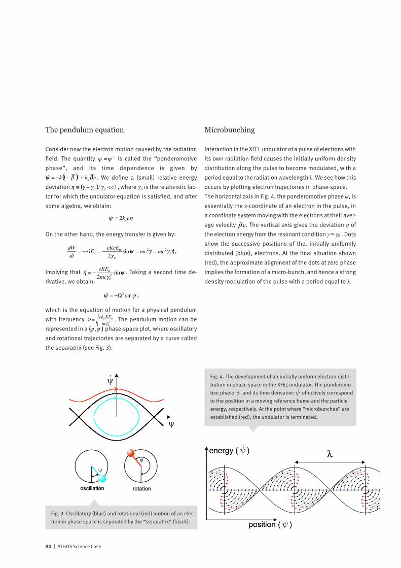
80 | ATHOS Science Case
The pendulum equation
Consider now the electron motion caused by the radiation field. The quantity
( ) ( )tEtxedtdW
x−=
x
Ex t( )= E0 cos kz−ωt+ψ0( ) ( )tx
( )−+ −−= ψψγ
sinsin2
0eKcEdtdW
( )[ ] ( )[ ]ββψψβψ uu kkcttkcckk −−=+−±=± 100 −ψ
−ψdtdW
const=+ψ
( )( )
( ) ⎟⎟⎠
⎞⎜⎜⎝
⎛+=−=
≈=−
=−
21
21
22121
2
2
K
kk
uu
uu
u
γλ
βλλ
λπ
βλπ
βλπ
ββ
+=ψψ
( ) ckck uββψ +−−= 1
( ) 1/ 00 <<−≡ γγγη 0γ
ηψ cku2=
ηγγψγ
022
0
0 sin2
mcmceKcE
ExedtdW
x ==−=−= ,
ψγ
η sin2 2
0
0
mceKE−=
ψψ sin2Ω−=
is called the “ponderomotive phase”, and its time dependence is given by
( ) ( )tEtxedtdW
x−=
x
Ex t( )= E0 cos kz−ωt+ψ0( ) ( )tx
( )−+ −−= ψψγ
sinsin2
0eKcEdtdW
( )[ ] ( )[ ]ββψψβψ uu kkcttkcckk −−=+−±=± 100 −ψ
−ψdtdW
const=+ψ
( )( )
( ) ⎟⎟⎠
⎞⎜⎜⎝
⎛+=−=
≈=−
=−
21
21
22121
2
2
K
kk
uu
uu
u
γλ
βλλ
λπ
βλπ
βλπ
ββ
+=ψψ
( ) ckck uββψ +−−= 1
( ) 1/ 00 <<−≡ γγγη 0γ
ηψ cku2=
ηγγψγ
022
0
0 sin2
mcmceKcE
ExedtdW
x ==−=−= ,
ψγ
η sin2 2
0
0
mceKE−=
ψψ sin2Ω−=
. We define a (small) relative energy deviation
( ) ( )tEtxedtdW
x−=
x
Ex t( )= E0 cos kz−ωt+ψ0( ) ( )tx
( )−+ −−= ψψγ
sinsin2
0eKcEdtdW
( )[ ] ( )[ ]ββψψβψ uu kkcttkcckk −−=+−±=± 100 −ψ
−ψdtdW
const=+ψ
( )( )
( ) ⎟⎟⎠
⎞⎜⎜⎝
⎛+=−=
≈=−
=−
21
21
22121
2
2
K
kk
uu
uu
u
γλ
βλλ
λπ
βλπ
βλπ
ββ
+=ψψ
( ) ckck uββψ +−−= 1
( ) 1/ 00 <<−≡ γγγη 0γ
ηψ cku2=
ηγγψγ
022
0
0 sin2
mcmceKcE
ExedtdW
x ==−=−= ,
ψγ
η sin2 2
0
0
mceKE−=
ψψ sin2Ω−=
, where
( ) ( )tEtxedtdW
x−=
x
Ex t( )= E0 cos kz−ωt+ψ0( ) ( )tx
( )−+ −−= ψψγ
sinsin2
0eKcEdtdW
( )[ ] ( )[ ]ββψψβψ uu kkcttkcckk −−=+−±=± 100 −ψ
−ψdtdW
const=+ψ
( )( )
( ) ⎟⎟⎠
⎞⎜⎜⎝
⎛+=−=
≈=−
=−
21
21
22121
2
2
K
kk
uu
uu
u
γλ
βλλ
λπ
βλπ
βλπ
ββ
+=ψψ
( ) ckck uββψ +−−= 1
( ) 1/ 00 <<−≡ γγγη 0γ
ηψ cku2=
ηγγψγ
022
0
0 sin2
mcmceKcE
ExedtdW
x ==−=−= ,
ψγ
η sin2 2
0
0
mceKE−=
ψψ sin2Ω−=
is the relativistic fac-tor for which the undulator equation is satisfied, and after some algebra, we obtain:
( ) ( )tEtxedtdW
x−=
x
Ex t( )= E0 cos kz−ωt+ψ0( ) ( )tx
( )−+ −−= ψψγ
sinsin2
0eKcEdtdW
( )[ ] ( )[ ]ββψψβψ uu kkcttkcckk −−=+−±=± 100 −ψ
−ψdtdW
const=+ψ
( )( )
( ) ⎟⎟⎠
⎞⎜⎜⎝
⎛+=−=
≈=−
=−
21
21
22121
2
2
K
kk
uu
uu
u
γλ
βλλ
λπ
βλπ
βλπ
ββ
+=ψψ
( ) ckck uββψ +−−= 1
( ) 1/ 00 <<−≡ γγγη 0γ
ηψ cku2=
ηγγψγ
022
0
0 sin2
mcmceKcE
ExedtdW
x ==−=−= ,
ψγ
η sin2 2
0
0
mceKE−=
ψψ sin2Ω−=
On the other hand, the energy transfer is given by:
( ) ( )tEtxedtdW
x−=
x
Ex t( )= E0 cos kz−ωt+ψ0( ) ( )tx
( )−+ −−= ψψγ
sinsin2
0eKcEdtdW
( )[ ] ( )[ ]ββψψβψ uu kkcttkcckk −−=+−±=± 100 −ψ
−ψdtdW
const=+ψ
( )( )
( ) ⎟⎟⎠
⎞⎜⎜⎝
⎛+=−=
≈=−
=−
21
21
22121
2
2
K
kk
uu
uu
u
γλ
βλλ
λπ
βλπ
βλπ
ββ
+=ψψ
( ) ckck uββψ +−−= 1
( ) 1/ 00 <<−≡ γγγη 0γ
ηψ cku2=
ηγγψγ
022
0
0 sin2
mcmceKcE
ExedtdW
x ==−=−= ,
ψγ
η sin2 2
0
0
mceKE−=
ψψ sin2Ω−=
,
implying that
( ) ( )tEtxedtdW
x−=
x
Ex t( )= E0 cos kz−ωt+ψ0( ) ( )tx
( )−+ −−= ψψγ
sinsin2
0eKcEdtdW
( )[ ] ( )[ ]ββψψβψ uu kkcttkcckk −−=+−±=± 100 −ψ
−ψdtdW
const=+ψ
( )( )
( ) ⎟⎟⎠
⎞⎜⎜⎝
⎛+=−=
≈=−
=−
21
21
22121
2
2
K
kk
uu
uu
u
γλ
βλλ
λπ
βλπ
βλπ
ββ
+=ψψ
( ) ckck uββψ +−−= 1
( ) 1/ 00 <<−≡ γγγη 0γ
ηψ cku2=
ηγγψγ
022
0
0 sin2
mcmceKcE
ExedtdW
x ==−=−= ,
ψγ
η sin2 2
0
0
mceKE−=
ψψ sin2Ω−=
. Taking a second time de-rivative, we obtain:
( ) ( )tEtxedtdW
x−=
x
Ex t( )= E0 cos kz−ωt+ψ0( ) ( )tx
( )−+ −−= ψψγ
sinsin2
0eKcEdtdW
( )[ ] ( )[ ]ββψψβψ uu kkcttkcckk −−=+−±=± 100 −ψ
−ψdtdW
const=+ψ
( )( )
( ) ⎟⎟⎠
⎞⎜⎜⎝
⎛+=−=
≈=−
=−
21
21
22121
2
2
K
kk
uu
uu
u
γλ
βλλ
λπ
βλπ
βλπ
ββ
+=ψψ
( ) ckck uββψ +−−= 1
( ) 1/ 00 <<−≡ γγγη 0γ
ηψ cku2=
ηγγψγ
022
0
0 sin2
mcmceKcE
ExedtdW
x ==−=−= ,
ψγ
η sin2 2
0
0
mceKE−=
ψψ sin2Ω−= ,
which is the equation of motion for a physical pendulum with frequency 2
0
0
γmKEeku=Ω
( )ψψ ,
ψ ψ
ψ
cβ
. The pendulum motion can be represented in a
20
0
γmKEeku=Ω
( )ψψ ,
ψ ψ
ψ
cβ
phase-space plot, where oscillatory and rotational trajectories are separated by a curve called the separatrix (see Fig. 3).
Microbunching
Interaction in the XFEL undulator of a pulse of electrons with its own radiation field causes the initially uniform density distribution along the pulse to become modulated, with a period equal to the radiation wavelength λ. We see how this occurs by plotting electron trajectories in phase-space.The horizontal axis in Fig. 4, the ponderomotive phase ψ, is essentially the z-coordinate of an electron in the pulse, in a coordinate system moving with the electrons at their aver-age velocity
20
0
γmKEeku=Ω
( )ψψ ,
ψ ψ
ψ
cβ . The vertical axis gives the deviation η of the electron energy from the resonant condition γ = γ0 . Dots show the successive positions of the, initially uniformly distributed (blue), electrons. At the final situation shown (red), the approximate alignment of the dots at zero phase implies the formation of a micro-bunch, and hence a strong density modulation of the pulse with a period equal to λ.
Fig. 3. Oscillatory (blue) and rotational (red) motion of an elec-tron in phase space is separated by the “separatrix” (black).
Fig. 4. The development of an initially uniform electron distri-bution in phase space in the XFEL undulator. The ponderomo-tive phase
20
0
γmKEeku=Ω
( )ψψ ,
ψ ψ
ψ
cβ
and its time derivative
20
0
γmKEeku=Ω
( )ψψ ,
ψ ψ
ψ
cβ
effectively correspond to the position in a moving reference frame and the particle energy, respectively. At the point where “microbunches” are established (red), the undulator is terminated.
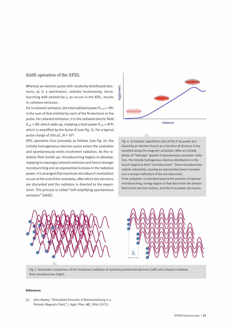
ATHOS Science Case | 81
SASE operation of the XFEL
Whereas an electron pulse with randomly-distributed elec-trons, as in a synchrotron, radiates incoherently, micro-bunching with periodicity λ, as occurs in the XFEL, results in coherent emission.For incoherent emission, the total radiated power Pincoh = NP1 is the sum of that emitted by each of the N electrons in the pulse. For coherent emission, it is the radiated electric field Ecoh = NE1 which adds up, implying a total power Pcoh = N2P1 which is amplified by the factor N (see Fig. 5). For a typical pulse charge of 200 pC, N ≈ 109!XFEL operation thus proceeds as follows (see Fig. 6): the initially homogeneous electron pulse enters the undulator and spontaneously emits incoherent radiation. As the ra-diation field builds up, microbunching begins to develop, implying increasingly coherent emission and hence stronger microbunching and an exponential increase in the radiation power. It is arranged that maximum microbunch modulation occurs at the end of the undulator, after which the electrons are discarded and the radiation is directed to the experi-ment. This process is called “self-amplifying spontaneous emission” (SASE).
�
Fig. 5. Schematic comparison of the incoherent radiation of randomly positioned electrons (left) and coherent radiation from microbunches (right).
Fig. 6. Schematic logarithmic plot of the X-ray power pro-duced by an electron bunch as a function of distance it has travelled along the magnetic undulator. After an initially phase of “lethargic” growth of spontaneous undulator radia-tion, the initially homogenous electron distribution in the bunch begins to form “microbunches”. These microbunches radiate coherently, causing an exponential power increase and a sharper definition of the microbunches. If the undulator is extended beyond the position of optimal microbunching, energy begins to flow back from the photon field to the electron motion, and the X-ray power decreases.
References
[1] John Madey, “Stimulated Emission of Bremsstrahlung in a Periodic Magnetic Field,” J. Appl. Phys. 42, 1906 (1971).
82 | ATHOS Science Case
DataAcquisition&ScientificComputing,Villigen:19.06.12
M. van Daalen (PSI) Introduction and welcomeB. Patterson (PSI) Goal of the workshopA. Perazzo (LCLS) Experience from LCLSK. Wrona (EU XFEL) Experience from EU XFELT.Griffin (ISIS) Experimental Metadata iCATJ. Krempsky (PSI) FEL ecperiments speaking EPICST. White (CFEL, DESY) Analysis pipeline for crystallographic data from FELs
Instrumentationworkshop:nextfrontierSwissFELinstruments,Villigen,22.05.2012
B. Patterson (PSI) IntroductionT. Schmitt (PSI) Time-resolved Resonant Inelastic X-Ray ScatteringS. Vaucher (EMPA) Microwave-induced materials dynamicsC. Gutt (DESY) X-ray Photon Correlation SpectroscopyB. Larsen (Oak Ridge Nat. Lab) Ion-implant pump / diffuse scattering probe studies of radiation defectsR. Röhlsberger (DESY) Nano-eV science at the 57Fe Mössbauer resonanceG. Knopp (PSI) Four-Wave Mixing at X-ray Wavelengths
SwissFELworkshop1:Spectroscopicexperiments,UniversityofBern,12.09.2011
B. Patterson (PSI) IntroductionH. Braun (PSI) The SwissFEL MachineR. Abela (PSI) SwissFEL Photonics
Discussions on poster presentations:B. Patterson (PSI) Mössbauer spectroscopic methods at the SwissFEL R. Thierry (Uni Basel) Constrained optimisation methoads for the retrieval of structural information in electron crystallography with limited tilt anglesJ. Szlachetko (PSI) Single-shot X-ray emission spectroscopy J. Sa (PSI) Photocatalytic conversion of CO2 to hydrocarbons over metal doped TiO2: artificial photosynthesisB. Patterson (PSI) Stimulated resonant inelastic X-Ray scattering P. Oberta The preliminary optics design of the Aramis undulator beamline of the SwissFEL A. Mozzanica (PSI) Adaptive gain charge integrating detectors for SwissFELC.Milne (PSI) Electronic and structural dynamics in solution: Pump-probe XAS, XES, RIXS P. Juranic (PSI) The basic concepts for photon beam diagnostics in the SwissFEL tunnel front end
Appendix
The ATHOS Science Workshop Series

ATHOS Science Case | 83
W. Gawelda (EU XFEL) Simultaneous Utrafast X-ray Spectroscopy and Scattering at Current and Future LightsourcesC. Hauri (PSI) Pump-probe laser systems at SwissFEL for ARAMIS hard X-ray beamlines A. Ichsanow (PSI) Initiation of catalytic reactions by THz pulses and characterization of short-lived internediate states by X-raysR. Ischebeck(PSI) Terahertz Streak Camera as Arrival Time Monitor for SwissFELM. Brown (ETHZ) Fast moving liquid interfaces for FEL studies: Spectroscopy, scattering and diffraction experiments
Time-ResolvedSpectroscopyonCorrelatedElectronMaterials,Zurich,6.3.09
F. Mila (EPFL) Correlated electron systems and XFELB. Batlogg (ETHZ) Electron Correlation – MaterialsU. Staub (PSI) Time Dependent Resonant Soft X-Ray DiffractionH. Dil (Uni ZH, PSI) Time, Spin, Space and Angle Resolved Photoemission on correlated (and other) systemsT. Schmitt (PSI) Pump and Probe Resonant Inelastic X-Ray Scattering at a Soft X-Ray FELS. Johnson (PSI) Femtosecond x-ray diffractionP. van Loosdrecht (Groningen) Correlated matter - Time resolved opticsD. van der Marel (Uni GE) THz spectroscopy: Polaron liquid in electron doped strontium titanate
CrazyIdeasandChallenges:ScienceIssues,Villigen,27.2.09
G. Ingold (PSI) Towards Pump-Probe Resonant Diffraction: 100-10 fsC. Spielmann (Jena) Femtosecond X-ray scienceS. Doniach (Stanford) 2-wave mixing in Mössbauer CrystalsA. Chumakov (Grenoble) XFEL spectroscopy at the Mössbauer resonanceM. Hengsberger (Uni ZH) Time-resolved photoelectron spectroscopy at x-ray energies using a time-of-flight spectrometer with spin analysisP. Abbamonte (Illinois) Inelastic x-ray scattering with [crazy] coherent FEL pulsesM. Howells (Berkeley) Toward a Modern Version of Fluctuation Scattering
Sub-psSolutionChemistryandSurfaceCatalysis,Lausanne,10.10.08
M. Nielsen (Copenhagen) Time-resolved X-ray scattering of an electronically excited state in solutionM. Meuwly (Uni Basel) Rapid Processes in [Biophysical] Chemistr yJ.-E. Moser (EPFL) Dynamics of light-induced interfacial electron transfer
84 | ATHOS Science Case
E. Aziz (BESSY) Toward Ultra-Fast Dynamics in SolutionsC. Milne (PSI) Ultrafast x-ray spectroscopies for the study of structural dynamics in molecular systemsM. Wolf (F-U Berlin) Ultrafast sur face femtochemistry and electron-phonon couplingC. Bressler (EPFL) Exploiting Hard X-Ray Spectroscopies at XFELsB. Zietz (EPFL) Simulated scattering in solutionJ. van Bokhoven (ETHZ) Structure of catalytically active sitesN. Bukowiecki (EMPA) Bulk analysis of solids using XRFM. Amman (PSI) Can a XFEL shed light on atmospheric particles?G. Knopp (PSI) Prospective experiments on catalytic surfaces
NanoscaleMagnetizationDynamics,Bern,5.6.08
R. Allenspach (IBM) XFEL for Magnetism StudiesR. Hertel (Julich) Magnetic vortex core dynamics – ultrafast and smallH. Brune (EPFL) Open Issues in Magnetic NanostructuresP. Gambardella (Barcelona) Magnetic spectroscopy @ XFELC. Back (Regensburg) Laser Induced Magnetization DynamicsM. Kenzelmann (ETHZ, PSI) Nanoscale Magnetization DynamicsC. Quitmann (PSI) Ideas for XFEL Science – Magnetization DynamicsH. Ronnow (EPFL) Mesoscopic dynamics in correlated electron materials – XFEL dreamsA. Vaterlaus (ETHZ): Magnetism far from equilibrium probed with Spin Polarized Photoemission
InformationDayontheUseofX-RayFreeElectronLasers,Bern,20.4.07
R. Eichler (PSI) IntroductionA. Wrulich (PSI) The PSI-XFEL projectM. Chergui (EPFL) Ultrafast X-ray science with free electron lasersR. Falcone (Berkeley) Research needs for a new generation of X-ray sources
Ideas for use of an XFEL: V. Sandoghdar (ETHZ) F. Pfeiffer (PSI) H.W. Fink (Uni ZH) M. Schiltz (EPFL) T. Richmond (ETHZ) P. Hamm (Uni ZH) G. Ingold (PSI) T. Feurer (Uni BE) C. Bressler (EPFL) A. Devaux (Uni BE)
Published byPaul Scherrer Institut
CoordinationRafael Abela
Images© Paul Scherrer Institut
Printing Paul Scherrer Institut
Available fromPaul Scherrer InstitutCommunications Services5232 Villigen PSI, SwitzerlandPhone +41 56 310 21 [email protected]
Copying is welcomed, provided the source is acknowledged and an archive copy sent to PSI.Paul Scherrer Institut March 2014

Paul Scherrer Institut :: 5232 Villigen PSI :: Switzerland :: Tel. +41 56 310 21 11 :: Fax +41 56 310 21 99 :: www.psi.ch