TIME RESOLVED FILTERED RAYLEIGH SCATTERING MEASUREMENT OF A CENTRIFUGALLY LOADED BUOYANT JET

THESIS

Firas Benhassen, 1st

Lt, TUNAF

AFIT/GAE/ENY/11-M01

DEPARTMENT OF THE AIR FORCE AIR UNIVERSITY

AIR FORCE INSTITUTE OF TECHNOLOGY

Wright-Patterson Air Force Base, Ohio

APPROVED FOR PUBLIC RELEASE; DISTRIBUTION UNLIMITED

The views expressed in this thesis are those of the author and do not reflect the official policy or position of the United States Air Force, Department of Defense, the United States Government, the Tunisian Air Force, nor the Tunisian Government. This material is declared a work of the U.S. Government and is not subject to copyright protection in the United States.

AFIT/GAE/ENY/11-M01

TIME RESOLVED FILTERED RAYLEIGH SCATTERING MEASUREMENT OF A CENTRIFUGALLY LOADED BUOYANT JET

THESIS

Presented to the Faculty

Department of Aeronautics and Astronautics

Graduate School of Engineering and Management

Air Force Institute of Technology

Air University

Air Education and Training Command

In Partial Fulfillment of the Requirements for the

Degree of Master of Science in Aeronautical Engineering

Firas Benhassen, BS

1st

Lt, TUNAF

March 2011

APPROVED FOR PUBLIC RELEASE; DISTRIBUTION UNLIMITED

iv

AFIT/GAE/ENY/11-M01

Abstract

The combustion process within the Ultra-Compact Combustor (UCC) occurs in the

circumferential direction. The presence of variable flow density within the circumferential

cavity introduces significant buoyancy issues. On the other hand, G-loading caused by the

presence of centrifugal forces, ensures the circulation of the flow in the circumferential cavity

and enhances the completion of the combustion process before allowing the exit of the hot gases

to the main flow. The coupling between buoyancy and high G-loading is what predominately

influences the behavior of the flow within the UCC. In order to better understand the

combustion process within the UCC, three different experiments were run. The overall objective

of these experiments is to investigate the effects of both buoyancy and G-loading on the

trajectory and the mixing of a jet in a co-flow. The first experiment involved setting up the

Filtered Rayleigh scattering (FRS) technique to be used in this research. Then, using horizontal

and curved sections, two types of experiments were run to characterize and measure both G-

loading and buoyancy effects on the overall behavior of a jet in a co-flow of air. Measurements

were made using a FRS set up which involved a continuous wave laser and a high speed camera

showing adequate signal to noise ratio at 400 Hz. Collected time resolved images allowed for

the investigation of the effects of G-loading and buoyancy on the mixing properties and

trajectory of the jet.

v

AFIT/GAE/ENY/11-M01

To my mother and my father

vi

Acknowledgments

I would like to express my gratitude and appreciation to the following individuals without

whom this work would not have been made possible. First of all, special thanks go to my thesis

advisor Dr. Marc Polanka for his support and patience throughout this entire program. I would

also like to thank Dr. Mark Reeder for his insight and specific guidance. My sincere thanks as

well, go to Captain Kenneth LeBay for his patience and willingness to give up countless hours of

his research time to help me with my experiments in the COAL lab. I would also like to thank

Mr. Jay Anderson and the technicians John Hixenbaugh, Chris Zickerfoose, and Brian Crabtree

for their technical support. I would also take this opportunity to thank Mr. Jacob Wilson and

Mr. Samuel Raudabaugh for helping me with SolidWorks. And last, but not least, I would like

to the Mrs. Annette Robb, the director of the International Military Student Office (IMSO) and

her technician Mr. Rorey Kanemoto for their time, efforts, and continuous support in all matters.

Firas Benhassen

1st

Lt, Tunisian Air Force

vii

Table of Contents

Page

Abstract .......................................................................................................................................... iv

Acknowledgments .......................................................................................................................... vi

Table of Contents .......................................................................................................................... vii

List of Figures ................................................................................................................................ ix

List of Tables ............................................................................................................................... xiii

I. Introduction ............................................................................................................................. 1

I.1. Background ...................................................................................................................... 1

I.2. Problem Statement ........................................................................................................... 3

I.3. Objectives ......................................................................................................................... 5

I.4. Implications ...................................................................................................................... 6

II. Literature Review ................................................................................................................. 7

II.1. Rayleigh-Scattering .......................................................................................................... 7

II.2. Effects of Buoyancy and G-loading on a Jet’s Behavior ............................................... 14

II.2.1. Buoyant Jets ............................................................................................................ 14

II.2.2. G-loaded jet ............................................................................................................. 21

II.3. Literature Review Findings and Unanswered Questions ............................................... 24

III. Methodology ...................................................................................................................... 26

III.1. Equipment ................................................................................................................... 26

III.1.1. Laser .................................................................................................................... 26

III.1.2. Iodine Filter ......................................................................................................... 27

III.1.3. Power meters ....................................................................................................... 28

III.1.4. Mass Flow Controllers ........................................................................................ 30

III.1.5. Camera ................................................................................................................ 32

III.1.6. Optics .................................................................................................................. 33

III.1.7. Wave meter and Accessories ............................................................................... 37

III.2. Experiment # 1: Iodine Filter Characterization .......................................................... 40

III.3. Experiment # 2: Horizontal Buoyant Jet in a Co-flow ............................................... 44

viii

III.4. Experiment # 3: G-loaded Buoyant jet in a Co-flow .................................................. 48

III.5. Buoyant Jet Experimentation Methodology ............................................................... 53

III.5.1. Data Acquisition Considerations ......................................................................... 53

III.5.2. Doppler Effect Considerations ............................................................................ 55

III.5.3. Data Processing ................................................................................................... 56

IV. Results and Analysis .......................................................................................................... 66

IV.1. Experiment # 1 : Iodine Filter Characterization ......................................................... 66

IV.2. Experiment # 2: Horizontal Buoyant Jet in a Co-flow ............................................... 73

IV.2.1. Cases With Helium Gas ...................................................................................... 73

IV.2.2. Cases With CO2 Gas ........................................................................................... 78

IV.3. Experiment # 3: G-loaded Buoyant Jet in a Co-flow ................................................. 98

V. Conclusions ...................................................................................................................... 111

V.1. Findings ........................................................................................................................ 111

V.2. Recommendations & Future Work .............................................................................. 113

Bibliography ............................................................................................................................... 115

Vita .............................................................................................................................................. 118

ix

List of Figures

Page

Figure 1. Conceptual (Left) and Actual AFRL UCC Model (Right) .............................................. 3Figure 2. UCC Integration with Turbine Vanes (modified) ........................................................... 5Figure 3. Rayleigh Scattering Spectrum (as inspired by Mielke et al.’s figure) ............................ 8Figure 4. Diagram of a Typical Filtered Rayleigh Scattering Set Up (as inspired by Miles et al.’s figure) .............................................................................................................................................. 9Figure 5. Illustration of the FRS Concept (as inspired by Miles et al.’s figure) ......................... 11Figure 6. Iodine Filter Absorption Well Characterization ............................................................ 13Figure 7. Helium Jet Cross Section for Fr = 0.71 and Re = 100 .................................................. 17Figure 8. Filtered Rayleigh Scattering Data of a Buoyant Jet Flowing at 7.5 SLPM of He ......... 17Figure 9. Filtered Rayleigh Scattering data of a Buoyant Jet Flowing at 1 SLPM of CO2 .......... 17Figure 10. CO2 Jet Cross Section for Fr = 0.71 and Re = 100 ..................................................... 18Figure 11. UCC Sections: Curved (Left) and Straight (Right) ..................................................... 22Figure 12. Chemiluminescence and Shadowgraph Images for ac=0, ac>0, and ac<0 ................. 23Figure 13. Coherent Verdi V12 Laser System ............................................................................. 27Figure 14. Iodine Filter and Accessories ...................................................................................... 28Figure 15. Orion, Vega, and Coherent Fieldmaster Power Meters ............................................... 28Figure 16. Power Meter Sensor .................................................................................................... 29Figure 17. The Brooks Instrument 5850i Mass Flow Controller ................................................. 30Figure 18. The Brooks Instrument 5853i Mass Flow Controller ................................................. 31Figure 19. Phantom V12.1 Camera .............................................................................................. 32Figure 20. Camera User Interface Software Screen Shot ............................................................ 33Figure 21. High Reflective (HR) Mirror ....................................................................................... 33Figure 22. Beam Splitters (or Samplers) ....................................................................................... 34Figure 23. Aperture and Unwanted Beam Spray .......................................................................... 35Figure 24. Spherical Lenses .......................................................................................................... 36Figure 25. Sheet of Laser in front of the Iodine Filter .................................................................. 36Figure 26. A LEO Density Filters ................................................................................................ 37Figure 27. WS-7 Wavemeter Unit ............................................................................................... 38Figure 28. Bristol (Model 621) Wavemeter ................................................................................. 39Figure 29. Laser Calorimeter (Right) and Fiber Optic Cable (Left) ............................................ 39Figure 30. WS-7 Wavemeter Computer Interface and Data Display (currently the wavenumber is 18787.9380 cm-1 ) .......................................................................................................................... 40Figure 31. Iodine Filter Characterization Setup Diagram ............................................................. 41Figure 32. Photos Showing the Iodine Filter Characterization Experimental Set Up ................. 42Figure 33. Diagram of Horizontal Buoyant Jet Set Up ................................................................ 44Figure 34. Horizontal Buoyant Jet Set Up Photo for the CO2 Configuration ............................. 45Figure 35. Horizontal Buoyant Jet Set Up Photo for the Helium Configuration ......................... 45

x

Figure 36. Equipment Used to Feed in Both the Jet (CO2 and Helium) and Air. ....................... 46Figure 37. Traverse and Scissor Jack Unit and Accessories ........................................................ 48Figure 38. Diagram of G-loaded Buoyant Jet Set Up .................................................................. 49Figure 39. G-loaded Buoyant Jet Set Up Photo ........................................................................... 50Figure 40. Stainless Tube Used to Feed in the CO2 ..................................................................... 50Figure 41. Curved Section CAD Drawing ................................................................................... 51Figure 42. G-loaded Buoyant jet Horizontal Area of Focus ......................................................... 51Figure 43. G-loaded Buoyant jet: Air Collection Chamber .......................................................... 52Figure 44. Frame Rate Sensitivity Analysis for the CO2 Jet Configuration ................................ 53Figure 45. Frame Rate Sensitivity Analysis for the Helium Jet Configuration ........................... 54Figure 46. Sensitivity of the Rayleigh Scattering Signal to the Doppler Effect. ......................... 56Figure 47. Unprocessed Image of Scattered Light of the Laser Going Through the CO2 Jet and Air at 400 Hz (Top) and the Grid Used for Spatial Reference (Bottom). ..................................... 57Figure 48. Sample Images of Signals Used for Data Processing of Both the CO2 and Helium Configurations ............................................................................................................................... 58Figure 49. Raw Rayleigh Scattering Image (Left) and Processed Concentration Plot (Right) for the CO2 Configuration .................................................................................................................. 61Figure 50. Raw Rayleigh Scattering Image (Left) and Processed Concentration Plot (Right) for the Helium Configuration ............................................................................................................. 61Figure 51. Sample CO2 Process Data: (a) Percent Concentration, (b) Concentration Profile, (c) Jet’s Trajectory .............................................................................................................................. 62Figure 52. Jet’s Concentration Profiles at 1.3 D .......................................................................... 63Figure 53. Position one (X/D=1.3): (a) Standard Deviation and (b) Mean ................................. 64Figure 54. Rayleigh-Scattering Signal Due to Air Associated with the First and Second Laser Beams: (a) Raw Images and (b) Intensity Counts ........................................................................ 65Figure 55. Repeatability Test of the Transmitted Power of the Filter at 90 o C ............................ 66Figure 56. Repeatability Test of the Transmitted Power of the Filter at 40 o C ............................ 67Figure 57. Iodine Filter Absorption Well for Three Different Cell Temperature ......................... 68Figure 58. Iodine Filter Absorption Well at 90o C ....................................................................... 69Figure 59. Iodine Filter Absorption Well with Respect to Wavelength in Air ............................ 70Figure 60. Iodine Filter Absorption Well with Respect to Wavelength in Vacuum .................... 70Figure 61. Iodine Filter Absorption Well with Respect to Relative Frequency .......................... 71Figure 62. Investigation of the Upper End on the Absorption Well ............................................ 72Figure 63. Rayleigh-Scattering Signal Inside and Outside the Filter’s Absorption Well ............ 72Figure 64. Helium Jet Concentration Plots: (a) Without Co-flow (Case 1), and (b) With Co-flow (Case 2) ......................................................................................................................................... 74Figure 65. Standard Deviation of Helium Intensity: (a) Without Co-flow (Case 1) and (b) With Co-flow (Case 2) ........................................................................................................................... 75Figure 66. Helium Concentration Profiles: (a) Without Co-flow (Case 1) and (b) With Co-flow (Case 2) ......................................................................................................................................... 76

xi

Figure 67. Helium Jet Trajectory With Co-flow (Case 1) and Without co-flow (Case 2) ........... 77Figure 68. Comparing Case 1 of the Helium Configuration Trajectory Points to the Literature 78Figure 69. CO2 Jet Concentration Plots: (a) Without Co-flow (Case 1), and (b) With Co-flow (Case 2) ......................................................................................................................................... 80Figure 70. Standard Deviation of CO2 Intensity: (a) Without Co-flow (Case 1) and (b) With Co-flow (Case 2) ................................................................................................................................. 81Figure 71. CO2 Concentration Profiles: (a) Without Co-flow (Case 1) and (b) With Co-flow (Case 2) ......................................................................................................................................... 81Figure 72. Comparing Jet Trajectory for no Co-flow Cases (1, 3 and 5) and With Co-flow Cases (2, 4, and 6) ................................................................................................................................... 82Figure 73. Comparing Case 1 of the CO2 Configuration Trajectory Points to the Literature ..... 84Figure 74. CO2 Raw Data Images With Co-flow (Case 2) and Without Co-flow (Case 1) ........ 85Figure 75. Two Dimensional Standard Deviation Plots of: (a) Case 1 (Vjet = 0.305 m/sec, Vco-

flow = 0 m/sec), (b) Case 2 (Vjet = 0.305 m/sec, Vco-flow = 0.305 m/sec), and (c) Comparison of Case 1 and Case 2 ......................................................................................................................... 86Figure 76. Time Histories of Four Points on the First Line at 1.2 D in the Horizontal Direction for Case 2 (Vjet = 0.305 m/sec, Vco-flow = 0.305 m/sec). ............................................................... 87Figure 77. Time Histories of Points 3 and Point 4 of Case 2 (Vjet = 0.305 m/sec, Vco-flow = 0.305 m/sec). ........................................................................................................................................... 88Figure 78. Cross-Correlation of Point 4 to Point 3 of Case 2 (Vjet = 0.305 m/sec, Vco-flow = 0 m/sec) ............................................................................................................................................ 88Figure 79. Frequency Content of 20 Second Long Time History of Point 3 of Case 2 ............... 90Figure 80. Two Lines Cross- Correlation for Case 7 (Vjet = 0.153 m/sec, Vco-flow = 0.153 m/sec)

....................................................................................................................................................... 90Figure 81. Two Lines Cross- Correlation for Case 2 (Vjet = 0.305 m/sec, Vco-flow = 0.305 m/sec)

....................................................................................................................................................... 91Figure 82. Two Lines Cross- Correlation for Case 8 (Vjet = 0.610 m/sec, Vco-flow = 0.610 m/sec)

....................................................................................................................................................... 91Figure 83. Effects of Jet Velocity on the Jet’s Trajectory ............................................................ 93Figure 84. Effects of Froude Number on the Jet’s Trajectory ...................................................... 94Figure 85. Effects of Relative Velocity on the Jet’s Trajectory (Maintaining Fr = 3.45) ............ 95Figure 86. Effects of Velocity Ratio on the Jet’s Trajectory: (a) Vratio = 2.0 , (b) Vratio = 1.0 ..... 97Figure 87. Effects of Reynolds Number on the Trajectory .......................................................... 97Figure 88. Locations of the three Considered Points of Case 5 (G-loaded Jet) ............................ 99Figure 89. Time Histories of the Three Points of Figure 88 ....................................................... 100Figure 90. Case 11 Standard Deviation (Intensity Counts) Plot ................................................ 101Figure 91. CO2 Jet Concentration Plots for Gjet = 0.07: (a) Case 1 (With Co-flow) and (b) Case 2 (Without Co-flow) ...................................................................................................................... 102Figure 92. CO2 Jet Concentration Plots for Gjet = 4: (a) Case 9 (With Co-flow) and (b) Case 10 (Without Co-flow) ...................................................................................................................... 102

xii

Figure 93. CO2 Jet Concentration Plots for Gjet = 100: (a) Case 11 (With Co-flow) and (b) Case 12 (Without Co-flow) ................................................................................................................. 103Figure 94. CO2 Jet Concentration Plots for Gjet = 1000: (a) Case 15 (With Co-flow) and (b) Case 16 (Without Co-flow) ................................................................................................................. 103Figure 95. CO2 Concentration Profile for Gjet = 0.07: (a) Case 1 (With Co-flow) and (b) Case 2 (Without Co-flow) ...................................................................................................................... 104Figure 96. CO2 Concentration Profile for Gjet = 1: (a) Case 3 (With Co-flow) and (b) Case 4 (Without Co-flow) ...................................................................................................................... 105Figure 97. CO2 Concentration Profile for: (a) Case 5 (With Co-flow),(b) Case 6 (Without Co-flow), (c) Case 7 (With Co-flow), and (d) Case 8 (Without Co-flow) ....................................... 105Figure 98. CO2 Concentration Profile for Gjet = 4: (a) Case 9 (With Co-flow) and (b) Case 10 (Without Co-flow) ...................................................................................................................... 106Figure 99. Comparing Concentration Profiles at X/D = 3.4 ....................................................... 107Figure 100. CO2 Concentration Profile for: (a) Case 11 (With Co-flow),(b) Case 12 (Without Co-flow), (c) Case 13 (With Co-flow), and (d) Case 14 (Without Co-flow) ............................. 107Figure 101. CO2 Concentration Profile for: (a) Case 15 (With Co-flow), (b) Case 16 (Without Co-flow), (c) Case 17 (With Co-flow), and (d) Case 18 (Without Co-flow) ............................. 108Figure 102. Flow in a Curved Pipe, after Prandtl (as inspired by Schlichting et al.’s figure) .... 109

xiii

List of Tables

Page

Table 1. Measured vs Tabulated Cross Section Values (as given by Sneep et al.) ...................... 10Table 2. Processed Cases of Different Flow Conditions for the Helium Jet ................................ 73Table 3. Processed Cases of Different Flow Conditions for the CO2 Jet ..................................... 79Table 4. G-loaded Buoyant Jet Cases ........................................................................................... 98

1

TIME RESOLVED FILTERED RAYLEIGH SCATTERING MEASUREMENT OF A

CENTRIFUGALLY LOADED BUOYANT JET

I. Introduction

I.1. Background

The human life on earth is affected in many aspects by fluids. It is, in fact, impossible to

imagine life without air, water or blood which fuel most of the living organisms. The oil and all

its derivatives are the driving motors of technology and many industrial activities that sustain our

economy and daily lives. For hundreds of years, fluids have been the subject of continuous

interest for physicians, biologists, environmentalists, physicists, chemists, and engineers. The

ultimate objective of investigating the characteristics of a fluid flow (whether at gaseous or liquid

state) is to predict and possibly control its behavior. When performing these investigations,

scientists and engineers are interested in the mechanisms that trigger or prevent the occurrence of

specific patterns or changes within the flow. In fluid dynamics, the behavior of the fluid is

studied in relation with inertial, viscous, thermal, and buoyancy effects. This research will focus

closely on the dynamics associated with buoyant effects and characterize their contribution in

shaping the behavior of the fluid flow.

A jet is considered buoyant when it is discharged into a medium where a large density

gradient is present. The jet effective density depends on whether it is hotter or cooler than its

surrounding fluid. The density gradient can also be due simply to the presence of different

species in the medium [1]. Examples of situations or problems involving buoyant jets include

but are not limited to: the emission of pollutant into the atmosphere or oceanic waters, safety and

fire hazards associated with leakage of gases such as hydrogen into air [2], and heating issues

2

associated with an uneven temperature distribution within combustion systems. Therefore,

studying buoyancy effects proves to be of great importance when it comes to preventing

environmental hazards, tracking pollutant plumes, or improving combustion efficiency.

However, acquiring accurate analysis from these investigations is often a challenging task

due to the sensitivity of the flow properties (velocity, pressure, temperature, etc) to the

introduction of any intrusive probing device within the medium in question. Examples of

intrusive measuring devices include hot-wires, thermocouples, and pitot tubes. In addition to

their body influence on the flow, these devices cannot operate properly in harsh media of high

temperature and pressure such as within a combustion environment [3]. Laser techniques

however, are non-intrusive and prove to be capable of both high temporal and spatial resolution

[4]. The non-intrusive aspect of these diagnostic techniques allows for the investigation of the

flow properties within boundary layers or combustion zones [4]. Particle Image Velocimetry

(PIV) and Filtered Rayleigh Scattering (FRS) are two of the most important laser techniques

considered by the researches when studying flow properties. PIV involves shining a laser sheet

into a pre-seeded flow and taking a series of images using a camera at a known frame rate. 2D

velocity is then calculated by comparing consecutive frames and dividing the traveled distance

by the time difference between the frames [5]. On the other hand, FRS techniques do not require

the presence of seeds within the flow. This technique involves the use of a narrow-line

bandwidth laser along with a camera and a molecular filter used to block unwanted background

or dust particles interference.

More specifically, for FRS when a flow is illuminated with a laser beam (or sheet), light is

scattered due to the presence of particles within the flow. The intensity of the scattered light is

proportional to the cross section of the scattering particle or molecule and thus to the density of

3

the species [6]. Using a high speed camera, time resolved information can be obtained by

capturing scattered light images and constructing density fields [7]. The molecular filter is used

to absorb the scattered light resulting from the stationary particles and background noise while

allowing the scattered signal shifted and broadened by thermal and Doppler effects to be

transmitted [8]. In addition to density profiles, more flow properties can be obtained by relating

the frequency shift and the broadening of the signal to respectively the velocity and the

temperature of the scattering species [7] as it will be discussed in the literature review section.

The FRS technique along with the use of a high speed camera constitutes the basis of this

research and will be thoroughly described in the second chapter as part of the literature review.

Now that the overall background of the research is laid out, let us delve into the essence of this

study and start with its relevance from an aerospace engineering stand point.

I.2. Problem Statement

This research is initiated and sponsored by the Propulsion Directorate of the Air Force

Institute of Technology (AFRL) located at Wright Patterson Air Force Base. The global scope

within which falls this study is ultimately integrating the Ultra Compact Combustor (UCC)

concept with a Highly Efficient Embedded Turbine Engine (HEETE) program [9].

Figure 1. Conceptual (Left) and Actual AFRL UCC Model (Right)

4

The concept of the UCC (shown in Figure 1) stems from the need to develop a more

compact combustion unit that increases the engine’s thrust to weight ratio while maintaining a

comparable fuel efficiency and structural robustness. The thrust to weight ratio is increased by

the reduction of the overall weight of the engine as a direct result of the more compact design.

The basic idea is to inject fuel and air into a circumferential cavity where combustion occurs in

the presence of high G-loading caused by the spinning of the unit. The centrifugal effect forces

the unburned (cold/heavy) mixture to remain circulating within the cavity until combustion is

completed. The hot (light) combustion products are then driven by buoyancy effects out of the

circumferential cavity, through the radial vane cavity (RVC), and back to the main flow [10].

Combustion occurs within the circumferential cavity which creates a large density gradient due

to the presence of lighter than air hot products and heavier than air unburned reactants. This

density difference brings up buoyancy effects which are the driving forces of pushing the hot gas

out of the circumferential cavity. Buoyancy and G-loading effects are both important in the

combustion process. Hence, their unique interaction needs to be characterized as they both

influence the direction of the flow within the circumferential cavity. As it exits the

circumferential cavity, the hot gas encounters the main flow. Initially, this creates a jet in cross

flow situation that quickly transforms to a hot jet in a relatively cold co-flow as the mixture is

carried downstream by the main flow. In order to create an even temperature profile across the

turbine vanes and hence avoid burning the turbine blades, we need to understand the mechanism

that ensures the migration of the hot gas from the exit of the circumferential cavity and radically

down the turbine airfoils. This migration ensures the mixture of the hot gas with the colder main

flow and allows for cooling to occur [9]. As a result, it is apparent that buoyancy affects the

flow direction, mixture, and cooling process within the UCC.

5

Figure 2. UCC Integration with Turbine Vanes (modified)

Figure 2 shows a schematic of the UCC integration with turbine vanes. Whether the UCC

concept is integrated with a missile size engine, a fighter size engine, as an inter-stage turbine

burner (ITB), or as a main combustion unit between the compressor and turbine, there are

fundamental questions to be answered to ensure a successful integration [9]. These questions

underline the objectives of this research.

I.3. Objectives

The objectives of this study can best be described by finding the answer to the following

questions:

1. How does buoyancy affect the direction of the flow within the circumferential cavity?

2. Does G-loading work against or with buoyancy with respect to the mixing of the hot and

cold flow in the main cavity?

3. What is the trajectory of the exiting hot gas once it is co-flowing with the relatively

colder main flow?

6

The answers to these questions will be sought simultaneously from two collaborating

perspectives. The first one, ties the relevance of these objectives to the UCC integration and the

engineering aspect of the posed problems. The second set of objectives works towards

strengthening of fundamental concepts involving buoyant jets and highlights the academic values

of the investigation along with the use of time resolved FRS technique.

I.4. Implications

Knowing the direction of the flow at any sub-stage of the combustion will help optimize

the integration of the UCC with a fighter size turbo jet engine while ensuring structural

robustness of the turbine blades. The study of centrifugally loaded buoyant jet in the presence of

a co-flowing gas has not been thoroughly investigated by previous researchers which makes this

work original. The findings of this research will ensure a better understanding of the dynamics

governing a buoyant jet’s behavior. In addition, the use of the FRS techniques in conjunction

with a high speed camera will allow for the acquisition of time resolved concentration profiles.

In this manner, intermediate fluctuations and turbulence effects can be recorded, captured, and

analyzed. The contribution added by the time resolved aspect of the data acquisition in this

research will help understand the interaction between the jet and the co-flow. The time

resolution difference in data acquisition has drastic implications in the way we interpret physical

phenomena associated with the centrifugally loaded buoyant jet.

7

II. Literature Review

The relevance of any research stems from the understanding of the problem in hands and

the reported efforts put in to solve it. It is therefore critical to present selected previous studies

that put this work into context and strengthen its relevance. Specifically, this literature review

will be divided into three major parts. First, a theoretical background of the Rayleigh scattering

phenomenon and the Filtered Rayleigh scattering technique employed in this study is described.

Second, results from major studies characterizing the behavior of buoyant jets are briefly

presented. Lastly, the relevance of this work to the UCC and the effects of G-loading on the

buoyant jet behavior are introduced while referencing previous investigations.

II.1. Rayleigh-Scattering

The Rayleigh scattering phenomenon was first documented by the English physicist Lord

Rayleigh in the 19th

6

century. His studies aimed to understand the origin of the intensity and

color of the atmosphere [ ]. Rayleigh scattering pertains to the elastic scattering from molecules

as opposed to Mie scattering which is attributed to the scattering from particles [11]. The

analytical theory and model for Mie scattering was developed by Gustav Mie who distinguished

between the scattering of light by small particles (with diameters less than the wavelength of

light) and bigger particles and molecules [3]. Mie’s mathematical model indicated that the

intensity of the scattered light (I) caused by a single particle is proportional to the particle’s

diameter (d) and the inverse of the wavelength raised to the fourth as shown in Equation (1) [3].

Equation (1) offers an explanation to the origin of the blue color of the sky. Blue light has the

shortest wavelength of all the visible light wavelengths and hence scatters more than the other

lights such as red, green or yellow.

8

Rayleigh scattering builds on these principles by realizing that when light goes through a

gas, it is scattered by the molecules and particles present in the gas [11]. In order to formulate a

full developed theory that includes scattering from molecules, the diameter (d) is replaced by a

parameter called the total cross section and given the Greek symbol σss. Equation (1) is then

modified resulting in Equation (2) which relates the power of scattered (Ps) light to the incident

light intensity (Io 6) [ ]:

Figure 3. Rayleigh Scattering Spectrum (as inspired by Mielke et al.’s figure)

The amount of scattered signal (area under the curve in Figure 3), is proportional to the

cross section and hence to the density of the molecules. Furthermore, when light is scattered,

9

two things occur. First, the scattered light is shifted in frequency due to Doppler Effect. Second,

the scattered light line-width is broadened as shown in Figure 3 due to the increase of the kinetic

energy driven by the particles’ motion. Since the frequency shift is mainly due to the

translational motion of the molecules [11], the flow velocity can be measured by processing the

scattered light images at different locations. Velocity can be calculated using the Yeh and

Cummins equation (given by Equation (3) ) which relates the velocity V, the scattering angle θ,

the frequency shift νD, 7and the incident light wavelength λ [ ].

Figure 4. Diagram of a Typical Filtered Rayleigh Scattering Set Up (as inspired by Miles et al.’s figure)

The velocity V is the scalar component of the vector velocity in the direction to which the FRS is

sensitive as shown in Figure 4 [7]. Further discussion of the frequency shift and the Doppler

Effect will be presented in fourth chapter of this report.

In addition, the line width of the scattered signal turns out to be proportional to the flow

temperature (as shown in Figure 3). Quantitative values of temperature can be determined using

Equation (4) below [12]:

10

Equation (4) allows for the calculation of the temperature T, given the angle between the

illumination and detection (θ), the incident light wavelength (λ), the mass of the gas molecule

(m), the linewidth (∆f), and the Boltzman constant (k).

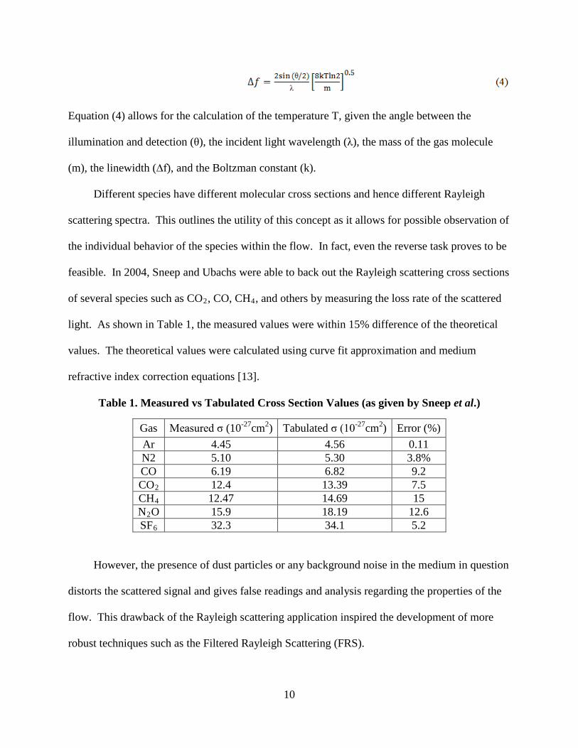
Different species have different molecular cross sections and hence different Rayleigh

scattering spectra. This outlines the utility of this concept as it allows for possible observation of

the individual behavior of the species within the flow. In fact, even the reverse task proves to be

feasible. In 2004, Sneep and Ubachs were able to back out the Rayleigh scattering cross sections

of several species such as CO2, CO, CH4

Table 1

, and others by measuring the loss rate of the scattered

light. As shown in , the measured values were within 15% difference of the theoretical

values. The theoretical values were calculated using curve fit approximation and medium

refractive index correction equations [13].

Table 1. Measured vs Tabulated Cross Section Values (as given by Sneep et al.)

Gas Measured σ (10-27cm2 Tabulated σ (10) -27cm2 Error (%) ) Ar 4.45 4.56 0.11 N2 5.10 5.30 3.8% CO 6.19 6.82 9.2 CO 12.4 2 13.39 7.5 CH 12.47 4 14.69 15 N2 15.9 O 18.19 12.6 SF 32.3 6 34.1 5.2

However, the presence of dust particles or any background noise in the medium in question

distorts the scattered signal and gives false readings and analysis regarding the properties of the

flow. This drawback of the Rayleigh scattering application inspired the development of more

robust techniques such as the Filtered Rayleigh Scattering (FRS).

11

In the FRS technique, a molecular filter is used to block scattered signal from walls,

windows, and particles and transmit only scattered light from molecules of interest as shown in

Figure 5 below. A filter should have steep cut off edges and allow for an overlap of frequencies

with the tunable laser in use [8].

Figure 5. Illustration of the FRS Concept (as inspired by Miles et al.’s figure)

12

The top graph of Figure 5 shows the background/particle scattering signal and the

molecular Rayleigh scattering signal. The bottom graph shows the absorption spectrum of the

molecular filter along with the transmitted Rayleigh scattering signal [8].

In their study on atomic and molecular notch filters, Miles et al. present three main criteria

for the selection of the filter [8].

a. Sharp cut off edges for high spectral resolution.

b. Deep absorption well that translates into almost 0% transmittance in the blocking

region and transmission close to 100% outside the absorption walls.

c. Overlap with tunable laser in use.

The molecular filter profile should be determined to optimize the collection of the scattered

light by tuning the laser to an adequate frequency. The goal is to make sure that most of the

scattered light (broadened and shifted) fall outside the absorption well of the filter while ensuring

near total absorbance of the incident signal itself, the background noise, and Mie scattering

(scattering due to particles). An iodine filter will be used for this research along with the

Coherent Verdi V12 continuous wave (CW) laser at 532 nm. The iodine filter is recognized for

having many transitions throughout the visible portion of the frequency spectrum. Figure 6

below illustrates the transmission curve of an iodine filter using a 7W continuous wave Coherent

Innova Sabre R Argon ion laser at 514 nm [14]. It is important to note that the higher the

temperature of the cell, the deeper the absorption well gets. In fact at 90o there is approximately

100% blocking (0% transmission) for a small range of wavenumber.

13

Figure 6. Iodine Filter Absorption Well Characterization

The equation for the intensity of light transmitted through a filter is given by Equation (5) :

Where I is the transmitted intensity, Io

8

the incident intensity, α is an absorption constant, l the

length of the filter, and V(w) a line width function that depends on the incident wavelength and

molecular collisions (i.e the temperature of the cell) [ ]. The take away of this equation is that

the filter’s absorption well depends on the temperature of the filter and the wavelength of the

incident light. It is necessary therefore to characterize the filter’s absorption well at 532 nm

before using it to ensure optimal Rayleigh scattering signal collection. The goal is to determine

the center line frequency of the absorption well as well as its width. As mentioned in the

methodology section of the first chapter, the characterization of the iodine filter at 532 nm is the

heart of the first experiment which will be fully discussed in Chapter Three of this report.

The relevance of the present work stems from the need to characterize the effects of

buoyancy and its governing parameters on the trajectory of a jet in a co-flow and its mixing

14

properties. The present work is based on a Filtered Rayleigh scattering (FRS) set up that allows

the capture of the intensity of the scattered light off of the molecules present in the testing area.

The fundamentals of the FRS are discussed throughout this work. This non intrusive technique

involves the use of a laser source, an iodine filter to block unwanted signal, and a camera to

capture the scattered light signal. In previous work, the use of a laser light along with a

molecular filter proved to be convenient when seeking either quantitative or qualitative mixing

measurements of gaseous flows. Jenkins and Desabrais used Planar Doppler Velocimetry (PDV)

to resolve velocity measurements within a low speed flow field [15]. The set up involved the use

of a tunable laser (Coherent Verdi V-18) in conjunction with three camera/iodine filter systems.

The iodine filters were used to discriminate the Doppler shifted scattered light (due to the motion

of the particles) from the un-shifted one. PDV is similar to FRS in the way that data is extracted

out of filtered scattered light using molecular cells such as the iodine cell used in this study.

In addition, one of the most recent studies in the literature pertaining to the acquisition of

time resolved concentration measurements in a gaseous flow is the work of Cheung and Hanson

in 2009. Using a tracer-based laser-induced fluorescence (LIF) diagnostic applied on a N2 jet

with 4% toluene (by mole fraction) issuing into air, the authors were successfully able to obtain

fluorescence signal time histories at a frame rate of 18.5 kHz using a continuous wave laser [16].

II.2. Effects of Buoyancy and G-loading on a Jet’s Behavior

This section will highlight the dynamics and mechanisms associated with a centrifugally

loaded buoyant jet as described in a collection of the most relevant reported efforts in this area.

II.2.1. Buoyant Jets

As mentioned in the introduction, the leading motive behind this research is to understand

the dynamics of a buoyant jet subjected to a G-loading in a combustion environment such as in

15

the case of the UCC. An important step toward understanding these dynamics deals with the

study of the fundamental concept of buoyancy and the researches associated with the behavior of

buoyant jets in different configurations (horizontal, vertical, G-loaded, etc) and various

environments such as combustive or cold medium.

In fluid dynamics, buoyancy is considered when a fluid with an initial momentum is

discharged into a medium where a density gradient is present. This gradient can be due to the

presence of various species or a difference in the temperature of the present entities (thermal

gradient) which alters their effective densities [17]. If we simply consider the behavior of an

impinging horizontal low density jet into a higher density medium, we anticipate the trajectory of

the jet to be influenced at least by inertial forces, body forces, density gradient, thermal gradient,

molecular diffusion, viscosity, and turbulence. Due to the coupling between all these physics,

buoyancy is usually described in the literature in terms of different parameters such as Reynolds

number, Froude number, Grashof number, and Richardson number. These parameters are

defined respectively as follows:

16

Where ρ is the jet density, D is the jet diameter, ν is the jet kinematic viscosity, V is the velocity

of the jet, Q is the volumetric flow rate, g is the gravitational acceleration, T is the jet’s

temperature, Ta

One effort in the literature that was fundamental to this research was the study performed

by Reeder et al. at AFIT in 2008 [

is the ambient temperature, and β is the coefficient of thermal expansion of the

jet.

18]. Its relevance stems from the use of FRS to collect

concentration measurements that allowed the investigation of the trajectory and the cross

sectional shape of a buoyant jet in ambient air. Both positive and negative buoyancy were

investigated using respectively horizontal jets of helium and carbon dioxide. In order to capture

images of the jet’s cross section, the authors used a continuous wave laser operating at a nominal

frequency of 514.5 nm wavelength, an iodine filter, and a PCO.4000 camera. The Froude

number was varied between 0.71 and 46 while the Reynolds number ranged from 50 to 1200.

The study acquired data at five different stream-wise locations to track the trajectory of the jet.

Figure 7 illustrates a sample raw picture of the helium jet cross section captured at x/D = 1.5

location. The helium jet is darker than the surrounding air spectrum since helium has a much

17

smaller cross section (only 1.4 % of that of air) than air [18] and hence scatters much less laser

light. Figure 8 and Figure 9, however, depict samples of the processed FRS images for both the

helium and CO2

jets.

Figure 7. Helium Jet Cross Section for Fr = 0.71 and Re = 100

Figure 8. Filtered Rayleigh Scattering Data of a Buoyant Jet Flowing at 7.5 SLPM of He

Figure 9. Filtered Rayleigh Scattering data of a Buoyant Jet Flowing at 1 SLPM of CO2

18

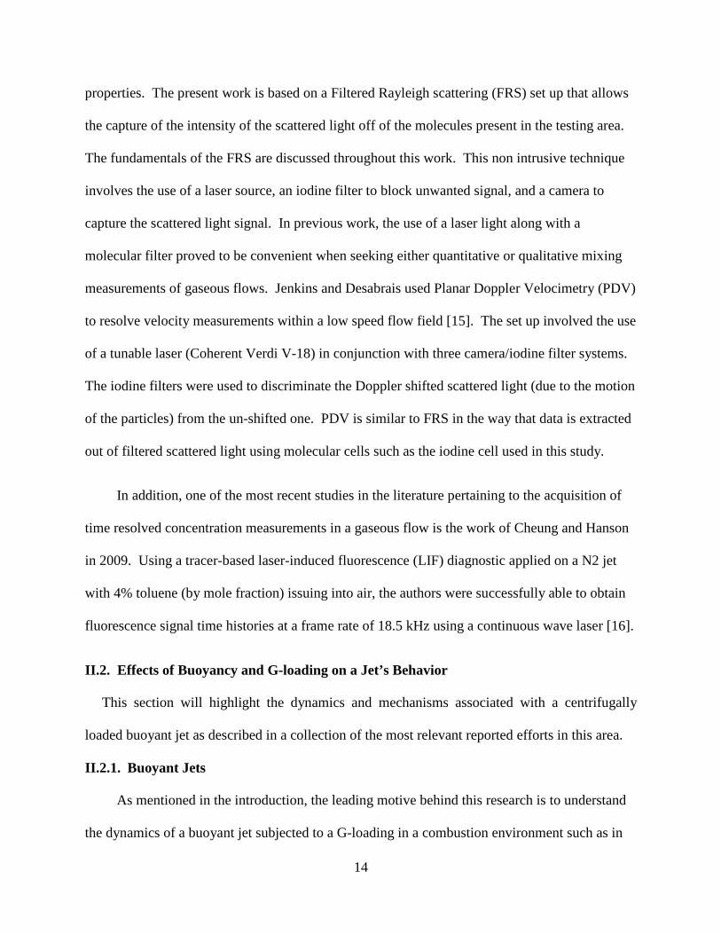
As expected, the lighter than air jet (helium) exhibited positive buoyancy while the heavier

than air jet (CO2) had negative buoyancy. In addition, it was noted that for values of Froude

number between 1.5 and 3 the jet’s cross section exhibits the formation of a plume (a tear drop

shape) ejecting from the core of the jet and directed upward for positive buoyancy (helium) and

downward for negative buoyancy (CO2 Figure 7). Raw images of these plumes are shown in

and Figure 10 for respectively the helium and CO2

jets.

Figure 10. CO2

The formation of these plumes for specific ranges of Froude number was also documented

by Arakeri et al. [

Jet Cross Section for Fr = 0.71 and Re = 100

19] in their study on buoyant horizontal laminar jet. Their set up was based on

“the injection of pure water jet in a brine solution.” The study showed that horizontal jets were

subjected to a bifurcation (formation of plumes) at low Froude number conditions between

values of 1 and 4.

In addition, it was noted that at sufficiently low Froude number (less than unity), the cross

section of the jet exhibited the formation of side lobes. For Froude number values less than unity

the tear drop shape was suppressed and two plumes (side lobes) emanated from the sides. This

behavior, which could clearly be seen in Figure 8 and Figure 9 above, was noted for both

positive and negative buoyancy. The formation of these lobes was more apparent at low values

19

of Froude number where buoyancy dominates inertia forces which underlines the effect

buoyancy has in shaping the cross section of the jet. In Reeder et al.’s study, the effect of inertia

on the shape of the jet’s cross section was also investigated through the variation of Reynolds

number. The study showed that the change in the shape of the plumes was minimal as Reynolds

number was changed. This suggests that the shape of the jet’s cross section is driven by

buoyancy rather than inertia [18]. Therefore, turbulence was not accounted for during these

tests. In fact, the sampling rate (1 Hz) was relatively low and would not have allowed for time

resolved images where turbulent effects could be observed.

Turbulence, however, was investigated by Subbarao in 1989 when he studied the behavior

of a buoyant jet as a function of Richardson and Reynolds numbers. The study involved taking

Schlieren photographs of a vertical helium jet as it was injected in a co-flowing air stream [1].

Cone-like structures were repeatedly seen in the Schlieren photographs and were essentially

vortex rings. These structures were the direct result of the interaction between buoyant forces

and the jet’s momentum. The vortex rings appeared to exhibit a constant periodicity for ranges

of Richardson number values between 1 and 4 and Reynolds number values between 260 and

900. The vortex rings became aperiodic for values of Richardson number greater than 5.

Furthermore, the study concluded that the higher the Richardson number (greater buoyancy), the

more accelerated the core jet (the cap of the cone) got and hence the more stretched out the cells

(cones) were. In addition, it was also noted that at higher Reynolds number the flow was more

turbulent which was expected. However, the transition from laminar to turbulent flow occurred

at a point closer to the jet exit as either Richardson number or Reynolds number increased which

indicated that the transition point was not solely affected by the Reynolds number but also by

buoyancy effects [1].

20

On a side note, it was noted that Subbarao used an absolute expression for the jet velocity

in the calculation of Richardson and Reynolds numbers even in the presence of a co-flowing air.

As it was mentioned earlier, this study will investigate the importance of the relative velocity of

the jet with respect to the co-flow when calculating buoyancy parameters. This will attempt to

understand how the Froude number should be defined in the presence of a co-flow since the

traditional definition does not include any term associated with a co-flowing jet. Testing will

compare the impact of changing both the absolute velocity range and the relative velocity

difference between the jet and the co-flow to understand the ongoing physics.

As documented by the literature, numerical and experimental studies involving hot and

cold impinging jets were carried out to characterize the effect of both aiding and opposing

buoyancy on the flow behavior. One of these investigations was the numerical study performed

by Kumar and Yuan in 1988 which involved simulating an impinging jet (both hot and cold) in a

rectangular cavity with constant wall temperatures. The conclusion of this study is that an

impinging cold jet encounters opposing buoyancy which prevents it from penetrating deeper

down the cavity. On the other hand, a hot jet penetrates all the way to the bottom of the cavity

due to the absence of opposing buoyancy (presence of aiding buoyancy). It was noted in this

analysis that a vortex was created on the bottom left corner of the cavity due to the presence of

two opposing flows (upward and downward) in the case of the cold jet while no vortex was

observed in the case of the hot jet [20].

A similar investigation was performed by Sherif and Pletcher in 1988 on aqueous turbulent

hot jet. The investigation confirmed the presence of a “kidney shaped” structure of the jet cross

section. The behavior of the flow was analyzed using contours of mean and fluctuations of

temperature across and along the jet. The contours were generated at velocity ratios of 1, 2, 4,

21

and 7. The authors discovered that the jet was more turbulent away from the centerline of the jet

(where the jet lost some of its momentum). In addition, the increase in the velocity ratio resulted

in a more pronounced and effective mixing of the jet and the streamline flow [21].

II.2.2. G-loaded jet

For the purpose of this research and its application on the UCC, the effect of G-loading on

the jet’s trajectory needs to be considered as well. In general, the G-load is given by Equation

(11) which is a relationship between the mass flow rate, the radius of curvature (r), the jet’s

density (ρjet

), and its cross sectional area (A). Within the UCC, the values of G-loading range

between 500 and 2000. The G-loading is controlled by varying the velocity of the jet or

essentially the mass flow rate. Equation (11) provides an expression for G-loading that will be

used in this study.

The U.S. Air Force Research Laboratory (AFRL) has been, since 2001, the leading party in

the conduction of studies and investigations geared toward gaining a better understanding of the

combustion process within the UCC. In 2004, Armstrong used the concept of

chemiluminescence to underline the effects of the centrifugal force on the combustion process

using the UCC test rig located in the AFRL’s Atmospheric Combustion Research Laboratory

[22]. The study involved running the UCC using the JP8+100 fuel and measuring the intensity

of light emitted by the three excited radicals C2* (excited C2), OH* (excited OH), and

CH*(excited CH) at eight different port locations in the inner and outer radius of the

circumferential cavity. The study showed that the intensities ratios CH*/OH* and C2*/OH*

were at their highest values at the ports in the outer radius of the circumferential cavity. This

22

indicated that the largest amount of fuel air mixture was reacting in the area of high G-loading

(the outer radius). Furthermore, it was noted that the intensity of C2* decreased as the G-loading

increased (going from inner to outer radius of the cavity). This trend indicated that the “higher

G-loadings reduced the residence time” which “could quench the C2 22* production” [ ].

In an additional effort to characterize the effects of G-loading on the combustion process,

the Air Force Institute of Technology’s Combustion Optimization and Analysis Laser (COAL)

Laboratory conducted a series of studies involving both a straight and a curved section of the

radial cavity as shown in

Figure 11. Using hydrogen as fuel, the G-loading was varied from 0 to

15000 g’s by controlling the mass flow rate and equivalence ratio. In order to capture the effects

of G-loading on the completeness of the combustion process, turbulent intensity, and temperature

profile, Particle Image Velocimetry (PIV) along with single-line and two-line Planar Laser-

Induced Fluorescence (PLIF) were used. The investigation revealed an increase in the turbulent

intensity with respect to G-loading. This led to the conclusion that the increase in centrifugal

force results in a better mixing, a reduction in chemistry time, and hence an advancement of the

combustion process. This conclusion was also underlined via the reduction of the amount of OH

in the main flow [23].

Figure 11. UCC Sections: Curved (Left) and Straight (Right)

23

In 2009, Lapsa and Dahm investigated the effects of positive and negative high centripetal

accelerations (up to 10,000 g’s) on both flame propagation and blowout limits using premixed

propane –air flames stabilized by backward step. The results of their study could simply be

summarized by Figure 12 which illustrates the chemiluminescence and shadow graph images

they acquired [24].

Figure 12. Chemiluminescence and Shadowgraph Images for ac=0, ac>0, and ac<0

The authors noted that in the case of positive acceleration, the buoyancy forces drove the

hot products (with lighter density) to the center of the turn and that the higher the centrifugal

24

force the better the mixing between hot and cold species was. However, in the case of negative

acceleration, the opposite scenario occurred. At higher (in absolute value) centripetal

acceleration, the separation between cold and hot gases was more pronounced which resulted in

less mixing. For both positive and negative acceleration, the study concluded an overall increase

in the flame propagation across the channel. Lastly, the authors discovered that the centripetal

force prevented the formation of large scale distortion and turbulence (as can be seen clearly in

Figure 12) which resulted in the stabilization of the flame and hence the increase of the blowout

speeds [24].

II.3. Literature Review Findings and Unanswered Questions

We deduce from the literature review that a horizontal buoyant jet (whether for positive or

negative buoyancy) is subjected to a bifurcation for a Froude number values between 1 and 4.

On the other hand, the center plume is suppressed from the core jet and replaced by two side

lobes for Froude number less than unity (Reeder et al.) [18]. These effects are less pronounced

for high values of Froude number (Fr>7) where the jet is momentum driven. Will these

observations still hold when a co-flowing air is introduced to the flow field? How will the

buoyant jet trajectory change when a co-flowing air stream is introduced? These are some of

the relevant and unanswered questions that the current research will attempt to answer.

Based on Subbarao’s study [1], the jet’s trajectory is characterized by the formation of

periodic and aperiodic vortex rings in the presence of a co-flowing air. The periodicity of these

structures is more apparent for 260 <Re<900 and 1 <Ri<4. Subbarao, however, was

investigating the classical case of a vertical jet. This study will investigate similar parameters,

however with initially a horizontal jet and later with a G-loaded jet. Will the horizontal jet in a

25

co-flow of air show the same structures? If so, is it possible to pick up the frequency of some of

these periodic structures in the presence of a co-flow?

Furthermore, we claim that in the circumferential cavity of the UCC, the cold unburned

fuel keeps circulating and being pushed outward until it is completely burned. This fact was

partially validated by Dahm’s study [24] which revealed that positive acceleration (positive g’s)

forced the heavier gas to move outward. Dahm’s research though was performed in a

combusting environment and did not consider the presence of a sustained flow. Then, how

would changing these conditions affect the direction in which the cold gas goes?

Investigating the behavior of the buoyant jet in the presence of a co-flow is one of the

fundamental objectives of this study. Particularly, this situation figures during the fuel injection

into the circumferential cavity. Based on Kumar and Yuan’s study [20], a hot flow injected in a

cold medium penetrates deeper than when a cold flow is injected into a hot environment due to

the absence (and respectively presence) of opposing buoyancy. In addition, at the same

Reynolds number (as a cold jet), the hot jet exhibits higher velocity since it has lower density.

This study however does not provide any details on the progression of the injected jet with

respect to time. Will it stay deeper in the cavity or eventually move upward? Sherif et al.’s

study [21] on the other hand, concluded that the increase in the jet to air velocity ratio resulted in

a more pronounced mixing between the jet and the cross-flowing air. Will this observation,

however, hold true in a more complex configuration where G-loading and co-flowing air effects

are introduced simultaneously?

The relevance of this research stems directly from the need to answer all these questions

which go in parallel with the list of objectives previously set in chapter one of this report.

26

III. Methodology

The methodology developed and executed for this research is outlined in this chapter.

Simply put, it entails setting up and performing three separate experiments that ensure the

collection of adequate data to answer the questions outlined in the research objectives. The first

experiment will be associated with properly setting up the FRS technique which requires the

characterization of the absorption well of the molecular filter to be used in the study. The second

and third experiments involve the use of FRS technique to collect jet concentration data using

two different configurations. The first configuration is based on a horizontal buoyant jet (helium

and CO2) in a co-flow of air. The second configuration (third experiment) involves the use of a

UCC like curved section with a circumferential cavity where air is flowing around a jet (CO2

III.1. Equipment

)

introduced in the cavity using a curved tube. The idea is to create an environment and a flow

structure that mimics the flow field within the UCC circumferential cavity. It is important to

note that all these configurations will have optical access from different views to allow the

capture of FRS images. These experiments along with the equipment are described in the

following sections.

The following sections will describe the equipment used in this research program. With the

exception of the mass flow controllers used in the third experiment for high flow measurements,

the same equipment is used for both the second and third experiment.

III.1.1. Laser

The laser used in this experiment is the Coherent VERDI Laser DPSS High Power CW

V12 manufactured by Coherent Inc. The laser outputs a maximum power of 12 W at a

wavelength of 532 nm. The lowest power it outputs is about 0.01 W. The laser system consists

27

of the laser head, a power supply and a water cooling unit as shown in Figure 13 below. The

laser’s wavelength can be tuned by changing the laser’s etalon temperature. Using the menu

display located on the power supply, the user can navigate through the different options. The

power can be regulated directly using a knob located next to the menu display. The laser can be

turned on using first an on/off switch on the back of the power supply, an enable/standby key ,

and a shutter switch located below the menu display.

Figure 13. Coherent Verdi V12 Laser System

III.1.2. Iodine Filter

As shown in Figure 14, the molecular filter used in this experience consists of a 3.5 inch

glass tube filled with iodine and a protective aluminum cylindrical case. It is manufactured by

Innovative Scientific Solutions Inc. (ISSI) of Dayton, Ohio.

Power supply

Water Cooler

Laser Head

Menu Display

28

Figure 14. Iodine Filter and Accessories

The filter is attached to a power supply cord and a thermocouple of type K. The

thermocouple is used to set the temperature inside the filter and is connected to a Cole-Parmer

Digi Sense control box.

III.1.3. Power meters

Figure 15. Orion, Vega, and Coherent Fieldmaster Power Meters

Iodine Cell

Cole-Parmer Digi Sense Control

Thermocouple

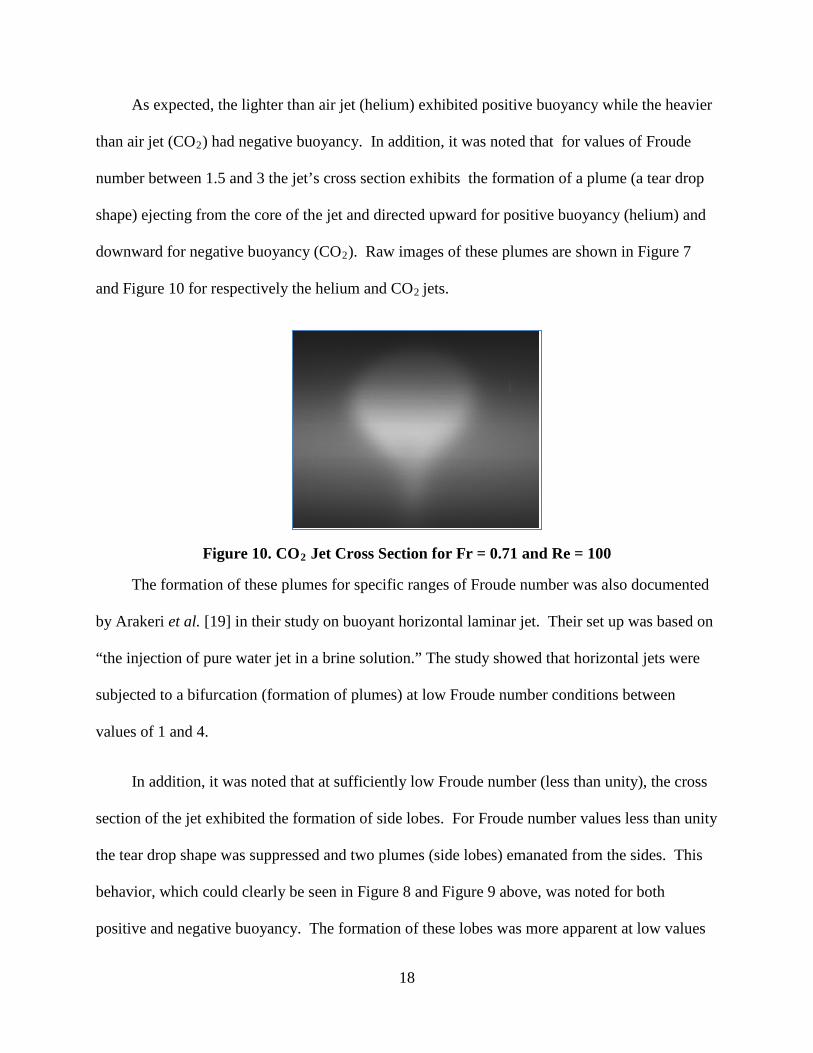
29

Three power meters were used during the iodine filter characterization experiment (Figure

15). Two of them (the Orion TH and the Coherent Fieldmaster) were used to acquire the

reference power and the transmitted power values. The third power meter was used to check the

consistency of the measurements during the experiment. Each power meter is attached to a

sensor and a power supply. A power meter sensor is shown in Figure 16 below. The Orion and

Vega meters are manufactured by the OHIR Laser Measurement Group. According to their

respective manuals, the Orion TH meter operating range is between 0.1 μW and 20 kW. The

Vega however measures values in range of nW and up to kW. Because the meters were of

different types, calibrating them was a necessary task. The meters were initially zeroed out with

the laser turned off. The Coherent Fieldmaster power meter has an accuracy of ±2%.

Figure 16. Power Meter Sensor

30

III.1.4. Mass Flow Controllers

For relatively low jet velocity measurements, the Brooks Instrument 5850i mass flow

controller shown in Figure 17 was used to control the jet mass flow rate to ±0.1SLPM. This flow

controller was calibrated for air at maximum flow rate value of 30 SLPM. For high flow

measurements, the Brooks Instrument 5853i mass flow controller, shown in Figure 18, was used

instead to control the jet’s mass flow rate to ±0.5 SLPM. This mass flow controller, however,

was calibrated for propane at a maximum flow rate value of 200 SLPM. The same user interface

(shown in Figure 17) was used to display and control the jet’s mass flow rate value.

Figure 17. The Brooks Instrument 5850i Mass Flow Controller

30 SLPM Mass Flow Controller (Calibrated for Air)

User Interface Unit

31

Figure 18. The Brooks Instrument 5853i Mass Flow Controller

For this research however, both mass flow controllers were intended to be used for Carbon

Dioxide (CO2) gas and helium. Equation (12) which is provided by the manufacturer is used to

relate the output reading and the actual value of the mass flow rates of the CO2

or helium jet.

As an example, when plugging the corresponding values for the conversion factors for the

cases when the Brooks 5850i were used for a CO2

jet, the relationship of Equation (12) becomes

Equation (13):

200 SLPM Mass Flow Controller (Calibrated for Propane)

32

III.1.5. Camera

Images used in this study were collected using a monochrome Phantom V12.1 (shown in

Figure 19) manufactured by Vision Research. This high speed camera enables image capture at

up to 1,000,000 Hz. For this research, data was captured at 400 Hz for the CO2

Figure 20

(and 80 Hz for

helium) jet allowing the capture of images at an adequate signal to noise ratio as will be

explained later on in this thesis report. In addition, this camera was also equipped with a Nikon

85mm lens with an f stop of 1.8. The camera has a maximum resolution of 1280x800 and an

exposure time down to 1μsec. All images have a pixel depth of 16 bit. illustrates a

snap shot of the camera software used to input the camera settings and initiate the data

collection.

Figure 19. Phantom V12.1 Camera

Nikon 85mm Lens (f/1.8)

33

Figure 20. Camera User Interface Software Screen Shot

III.1.6. Optics

Various optical tools were needed in this research to direct the laser beams to the test

section and control its power. The optics includes mirrors, beam splitters, density filters and

others as it will be discussed in this section.

III.1.6.1. Mirrors

Figure 21. High Reflective (HR) Mirror

34

High reflective mirrors were used in all three experiments to turn the beam 90o

Figure 21

. These

mirrors (shown in ) reflect 99% of the beam while letting only 1% goes through. The

mirrors are manufactured by Lattice Electro Optics (LEO), Inc.

III.1.6.2. Beam Splitters

The objective behind using a beam splitter (whether the 50-50 or the 90-10) is to reduce the

power of the beam to a predefined percentage. The beam splitters (or often called beam

samplers) used in the first experiment (the iodine filter characterization) are shown in Figure 22.

Both beam samplers are made by LEO and are designed to be used with a laser of a wavelength

value around 532 nm. The 50-50 beam splitter is a 2 inch diameter sampler. It divides the beam

into two perpendicular beams transmitting 50% of the incident power each. The 90-10 power is

a regular glass plate that allows 90% of the power to pass through while reflecting the remaining

10% at a 90o

angle.

Figure 22. Beam Splitters (or Samplers)

50-50 Beam Splitter

90-10 Beam Splitter

35

III.1.6.3. Aperture

The aperture was used in all three experiments. The intent behind using it is to block the

unwanted beam spray as shown in Figure 23. The laser power was set during the measurements

at 12 W. It is important at this high power to intercept and block any stray beams to avoid any

risks of burning any surface the laser may be in contact with. The aperture is manufactured by

ThorLabs.

Figure 23. Aperture and Unwanted Beam Spray

III.1.6.4. Spherical lenses

Two spherical lenses (shown in Figure 24) were used in the iodine filter characterization

experiment. Both lenses were manufactured by LEO. The first one (on the right) is a 1 inch

diameter, +25 mm spherical lens used to create a sheet of laser in front of the iodine filter to

allow for maximum passage through the inner volume of the filter. The 25mm is the focal length

Beam Spray

36

and indicates that the beam will be focused to a point at 25 mm behind the lens. Beyond the 25

mm, the beam is turned into a sheet as shown in Figure 25. The second spherical lens is a 2 inch

diameter, +200 mm lens and is used to focus the sheet of laser back to a point after passing

through the filter before it is intercepted by the power meter sensor.

Figure 24. Spherical Lenses

Figure 25. Sheet of Laser in front of the Iodine Filter

2 Inches

25 mm Spherical Lens

200 mm Spherical Lens

Iodine Filter

37

III.1.6.5. Density Filters

Two density filters were employed during the first experiment to further reduce the power

of the incident beam. One density filter with an opacity of 2.0 (98% absorption) is placed in

front of the wave meter sensor while the other one, with an opacity of 3.0 (99% absorption), was

positioned in front of the aperture in the way of the main beam directed toward the filter. The

two filters are manufactured by LEO. Figure 26 below shows one of the density filters used for

this experiment. Similarly to the other optical tools, the density filter is mounted on a ThorLabs

post.

Figure 26. A LEO Density Filters

III.1.7. Wave meter and Accessories

In order to keep track of the laser’s wavelength, two different wave meters were used

throughout this research. The first wavemeter used for the iodine filter characterization is a

HighFinesse WS-7 wave meter shown in Figure 27. The wave number (or wavelength) values

38

were acquired via the WS-7 software provided by the company TOPTICA. According to the

WS-7 user’s manual, the device is capable of measuring wavelength values in the range between

192 nm and 2250 nm. In addition, it can be used for both pulsed and continuous wave lasers.

When operating between 370 nm and 1100 nm, the device has an accuracy of 60 MHz which

corresponds to approximately 0.00005 nm.

Figure 27. WS-7 Wavemeter Unit

The second wave meter is the Brsitol Model 621 wavemeter. The Bristol wavemeter was

used in the second and third experiments. This wavemeter has comparable characteristics as the

WS-7 wavemeter mentioned earlier. Both wavemeters were connected to a computer using the

corresponding device’s USB interface. In addition, they were both used in conjunction with a

fiber optic cable attached to a calorimeter as shown in Figure 29. A screenshot of the computer

screen during the acquisition of the data when using the WS-7 wavementer (as an example) is

shown in Figure 30.

39

Figure 28. Bristol (Model 621) Wavemeter

Figure 29. Laser Calorimeter (Right) and Fiber Optic Cable (Left)

40

Figure 30. WS-7 Wavemeter Computer Interface and Data Display (currently the wavenumber is 18787.9380 cm-1

III.2. Experiment # 1: Iodine Filter Characterization

)

As mentioned in the literature review section, the molecular filter characterization is

essentially plotting the absorption well within which there will be blocking of the incident light.

Based on the diagram of Figure 5, maximum absorption (about 0% transmission) occurred for a

small range of frequency between a lower boundary value of wavenumber (or wavelength or

frequency) νmin and an upper boundary value νmax . The well is usually centered at a reference

frequency νo. The objective of the filter characterization experiment is therefore, determining

values of νmin and νmax of the absorption well centered at about 532 nm which corresponds to the

wavelength of the laser in use in this research. When testing, tuning the incident laser to a

frequency between νmin and νmax

Figure 31

ensures maximum blocking of undesired scattered light and

background noise. The experimental set up used to characterize the iodine filter is illustrated in

and Figure 32.

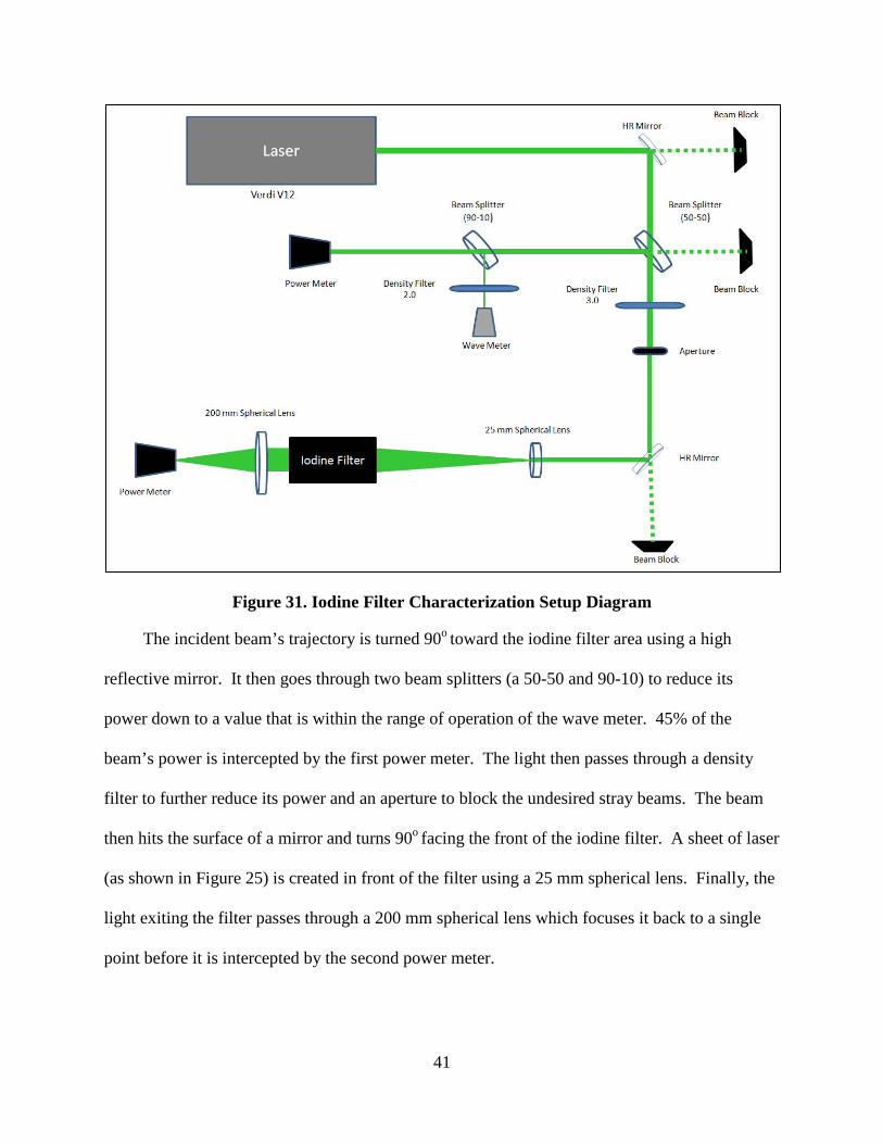
41

Figure 31. Iodine Filter Characterization Setup Diagram

The incident beam’s trajectory is turned 90o toward the iodine filter area using a high

reflective mirror. It then goes through two beam splitters (a 50-50 and 90-10) to reduce its

power down to a value that is within the range of operation of the wave meter. 45% of the

beam’s power is intercepted by the first power meter. The light then passes through a density

filter to further reduce its power and an aperture to block the undesired stray beams. The beam

then hits the surface of a mirror and turns 90o

Figure 25

facing the front of the iodine filter. A sheet of laser

(as shown in ) is created in front of the filter using a 25 mm spherical lens. Finally, the

light exiting the filter passes through a 200 mm spherical lens which focuses it back to a single

point before it is intercepted by the second power meter.

42

Figure 32. Photos Showing the Iodine Filter Characterization Experimental Set Up

The construction of the iodine filter absorption well is essentially plotting the percentage of

the transmitted power as a function of the wave number (or the wavelength, or the frequency).

Mirro 25 mm Spherical Lens

Iodine Cell

200 mm Spherical

Verdi V12 (532 nm)

Density Filters

Beam Splitters

Power Meter

Mirror

43

For that purpose, the power of the laser exiting the iodine filter was measured and the ratio of the

output to input power was calculated as the wavelength was changing. The wavelength can be

changed by varying the etalon temperature of the laser. This could be achieved using the

software interface associated with the V12. According to the user’s manual, the etalon

temperature can be varied between 35 oC and 75oC. For example, the command to set the etalon

temperature to 40o

> >et = 40

is given by:

The command to check the currently set etalon temperature is:

>>?est

It is important to note though that the wavelength (or the wave number) values decrease

spontaneously over time. Starting with a high value of wave number (way larger than the range

where the well is) allows for a slow drift that could be taken advantage of to record the values of

the corresponding transmitted power as the wave number decreases. This approach was used for

the iodine filter characterization in order to avoid changing the etalon temperature and obtain

more consistent results. For this experiment, the incident power was set at 1.04 W. According

to the V12 user’s manual, the power has to be greater than 5 % of the maximum output (12 W) to

avoid driving the laser to enter an alignment mode (where the power could not be accurately

measured). As mentioned in the Second Chapter, the well’s shape and depth change with

respect to the iodine cell temperature. Three different cell temperatures (40 o C, 60 o C, and 90o

C) were investigated during this experiment.

44

III.3. Experiment # 2: Horizontal Buoyant Jet in a Co-flow

The experimental set up to collect scattered light images off of a horizontal buoyant jet in a

co-flow is shown in Figure 33. In order to investigate the effects of both positive and negative

buoyancy on the jet’s trajectory and behavior, both helium and Carbon Dioxide (CO2) jets were

respectively used. Because the two gases have significantly different densities, two different

configurations of the plenum in which air flows, were used to create comparable test conditions.

The plenum section (for both helium and CO2 configurations) was designed by Mr. Samuel

Raudabaugh. In order to create comparable test conditions for these two configurations, the exit

area of the helium configuration plenum is about 60% smaller than that of CO2

Figure 34

as it could

clearly be noticed when comparing and Figure 35. The experimental set up however,

is essentially the same for both configurations.

Figure 33. Diagram of Horizontal Buoyant Jet Set Up

45

Figure 34. Horizontal Buoyant Jet Set Up Photo for the CO2

Configuration

Figure 35. Horizontal Buoyant Jet Set Up Photo for the Helium Configuration

46

For both configurations (helium and CO2

Figure 36

), the core jet flow is provided by a stainless steel

tube whose diameter can be varied to alter the Froude number and Reynolds number values. The

Brooks Instruments 5850i mass flow controller was used to control the jet mass flow rate. The

co-flow was delivered from an air tank through a mass flow controller that could be adjusted to

±0.01 kg/min. Air then entered a plenum made of Plexiglas via four orifices at which were

placed four washing nozzles to ensure a uniform flow of air. The co-flow passed through a

honeycomb screen with 9.5 mm openings (as shown in ) prior to passing through a

converging duct (the yellow box for the CO2

Figure 36

configuration and the metal one for the helium

case). The Plexiglas tank was sealed at one end using a 0.375’’ thick metal plate. As shown in

, a PVC fitting (going through the metal plate) was used to feed in the CO2

(or helium)

to the stainless tube.

Figure 36. Equipment Used to Feed in Both the Jet (CO2 and Helium) and Air.

Stainless Tube

Washing Nozzle PVC Fitting

Metal Plate

Honeycomb Screen

Plexiglas Tank

47

As mentioned earlier, the laser used for this study was a Coherent 12 W CW Verdi V12

with a wavelength around 532 nm. As shown in Figure 33, the beam was routed to the test

section using four highly reflective (HR) mirrors at 532 nm. The closest mirror to the tube

directed the laser vertically to a prism that reflected the beam back to the same mirror and then to

a beam block. This created two vertical laser beams intersecting with the jet and the co-flowing

air. The intent behind using two laser beams as opposed to a laser sheet (as used in previous

FRS studies) was to maintain the high power of the beams to maximize the scattered light

intensity known to be proportional to the incident light intensity. Using the Phantom V12.1 high

speed camera, data was captured at 400 Hz for the CO2

Before the scattered light was captured by the camera, it was filtered by the iodine cell

positioned in front of the camera. The temperature inside the filter was controlled by a Cole-

Parmer Digi Sense control box. The goal was to ensure that most of the scattered light

(broadened and shifted) fell outside the absorption well of the filter while ensuring near total

absorbtion of the incident signal itself, the background noise, and Mie scattering (due to

particles). In addition, a 200 mm spherical lens was placed in front of the iodine filter to

increase the effective focal length of the camera allowing for a better focus and hence a better

spatial resolution. The Bristol (Model 621) wavemeter (as shown in

(and 80 Hz for the helium) jet allowing

the capture of images at an adequate signal to noise ratio. The camera has a maximum resolution

of 1280x800 and an exposure time down to 1μsec. The camera was focused at the area of

intersection between the laser beams and the gases (both the jet and the co-flowing air).

Figure 28) monitored the

wavelength of the laser to ensure maximum absorbance of background noise by the filter.

Further, a slotted board minimized the background noise before reaching the filter.

48

In order to enable data collection at different stream-wise and vertical locations a traverse/

scissor jack unit was employed. As shown in Figure 37, the scissor jack (which is attached to

the Plexiglas tank) allowed for a maximum vertical range of 2.25’’. The traverse allowed for a

horizontal displacement of 2.3’’. The unit was controlled using a joy stick, an Anilam Wizard

150 power supply and a Questar digital readout.

Figure 37. Traverse and Scissor Jack Unit and Accessories

III.4. Experiment # 3: G-loaded Buoyant jet in a Co-flow

The experimental set up to collect scattered light images off of a G-loaded buoyant jet in a

co-flow is shown in Figure 38. The set up for this experiment involved, in general, the use of the

same equipment of the second experiment (horizontal jet). The straight configuration consisting

of the cubic plenum and the horizontal tube used in the second experiment, were replaced by an

SLA curved hallow section in which flowed air around a bent stainless tube as shown in Figure

39 and Figure 40. The shape of this curved section was designed by Mr. Jacob Wilson who

based his drawings on the actual UCC rig used in the COAL lab. The SLA section, of which a

Scissor Jack

Traverse

Joy Stick

Questar Readout

Power Supply

49

CAD drawing is shown in Figure 41, has a radius of curvature 38c m (15 inches) and a squared

cross section with 4.8 cm (1.9 inches) on each side. Three different tubes of different inner

diameters of 0.635 cm (0.250 inches), 0.775 cm (0.305 inches), and 1.09 cm (0.430 inches) were

used during this experiment. Due to the flow of the gases (both co-flowing air and the jet) along

the curvature of the section and the stainless tube, the gases were subjected to a normal outward

acceleration. Carbon Dioxide was used as a jet for this experiment to easily separate the effects

of buoyancy (pulling the jet down) and those of the G-loading (expected to push the CO2

molecules outwards).

Figure 38. Diagram of G-loaded Buoyant Jet Set Up

50

Figure 39. G-loaded Buoyant Jet Set Up Photo

Figure 40. Stainless Tube Used to Feed in the CO2

Stainless Tube

51

Figure 41. Curved Section CAD Drawing

Figure 42. G-loaded Buoyant jet Horizontal Area of Focus

This experiment was set up in a way such that the area of interest at which the camera was

focused was a horizontal section as shown in Figure 42. In order to allow the laser beams to pass

through the sides of the horizontal section and intersect with the jet and the co-flowing air, four

Horizontal Section (Area of camera focus)

52

different pieces of Quartz were used to seal the sides of the test section (the area of interest).

The laser was directed to the area of interest using the same optics used in the second

experiment. Imaging occurred along two vertical laser beams allowing the collection of intensity

(or concentration) data at two different stream-wise locations for each run. The curved section

was fixed on top of the traverse platform allowing the entire unit to move horizontally. This

enabled data collection at different stream-wise locations. The co-flow was delivered from the

same air tank used in the horizontal jet experiment. Before entering the curved section, air was

collected at a rectangular shaped chamber (shown in Figure 43). Through this chamber the

stainless tube was passed. The tube brought the jet of CO2

from the tank through the Brooks

mass flow controllers and to the measuring station. As mentioned earlier, the Brooks 5850i mass

flow controller was used for low velocity (and G-loading) measurements while the Brooks 5853i

mass flow controller was used for the high G-loading data collection.

Figure 43. G-loaded Buoyant jet: Air Collection Chamber

Air Chamber

Air Tube Jet Tube

Traverse Platform

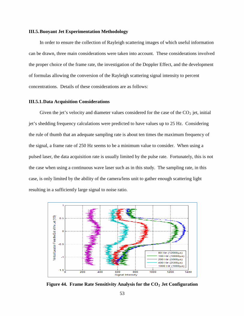
53

III.5. Buoyant Jet Experimentation Methodology

In order to ensure the collection of Rayleigh scattering images of which useful information

can be drawn, three main considerations were taken into account. These considerations involved

the proper choice of the frame rate, the investigation of the Doppler Effect, and the development

of formulas allowing the conversion of the Rayleigh scattering signal intensity to percent

concentrations. Details of these considerations are as follows:

III.5.1. Data Acquisition Considerations

Given the jet’s velocity and diameter values considered for the case of the CO2

jet, initial

jet’s shedding frequency calculations were predicted to have values up to 25 Hz. Considering

the rule of thumb that an adequate sampling rate is about ten times the maximum frequency of

the signal, a frame rate of 250 Hz seems to be a minimum value to consider. When using a

pulsed laser, the data acquisition rate is usually limited by the pulse rate. Fortunately, this is not

the case when using a continuous wave laser such as in this study. The sampling rate, in this

case, is only limited by the ability of the camera/lens unit to gather enough scattering light

resulting in a sufficiently large signal to noise ratio.

Figure 44. Frame Rate Sensitivity Analysis for the CO2 Jet Configuration

54

Inherently, the higher the frame rate, the smaller the exposure time is, and hence the

smaller the signal to noise ratio. Keeping this compromise in mind, it is therefore important to

perform a frame rate (or exposure time) sensitivity analysis to figure out the highest possible

frame rate value that would allow for an adequate signal to noise ratio. As shown in Figure 44, a

frame rate of a 1000 Hz results in a poor signal to noise ratio (N/S of 70%). At 400 Hz however,

it is easy to discern the Rayleigh scattering signal due to CO2

Figure 44

from the one due to air (N/S of

21%). The signal intensity shown in is the sum of raw intensity values of five adjacent

pixels. The signal due to CO2 molecules is higher than the one due to air molecules since the

CO2 molecule has larger Rayleigh scattering cross section than the air molecule as it will be

discussed in the data processing section of this thesis. Due to the fact that sampling rate and

exposure time are inversely proportional, the signal is much higher for frame rates lower than

400 Hz (N/S of 7 % at 80 Hz for instance). However, due to the shedding frequency

consideration discussed earlier, a frame rate of 400 Hz is chosen for the case of the CO2

jet.

Figure 45. Frame Rate Sensitivity Analysis for the Helium Jet Configuration

Similar analysis is performed to choose a data acquisition rate for the case of the helium

jet. There was no shedding frequency consideration in this case, since time resolved analysis

55

was only considered for the case of the CO2

Figure 45

jet due to time limitation. A data acquisition rate of

80 Hz (with a N/S of 25 % ) was considered for the case of the helium jet as it allows for the

balance between a relatively high frame rate and an adequate signal to noise ratio as shown in

. The noise to signal ratio (N/S) for both CO2

III.5.2. Doppler Effect Considerations

and helium measurement appears to be

high (about 25 %). However, this sensitivity analysis was based on raw intensity data. When

the intensity is converted to concentration, as will be explained in the data processing section, the

background signal is subtracted which eliminates a significant amount of noise. An uncertainty

analysis is performed in the data processing section to quantify the estimated percent error of the

collected data and analysis.

As mentioned in the literature review section, the Rayleigh scattering central frequency can

be Doppler shifted due to the motion of the molecules present in the flow. This shift, if not taken

into account, could drive the Rayleigh scattering signal out of the absorption well and hence give

false readings relating to the intensity of the signal. This study involves collecting Rayleigh

scattering signal of moving CO2,

υ∆

helium, and air molecules. Therefore, the Doppler Effect on

the measurements needs to be addressed. When associated with the Rayleigh scattering

phenomenon, the Doppler Effect, due to the motion of the molecules, results in a frequency shift

given by Equation (14):

As shown in the equation, the frequency shift is the dot product of the jet velocity vector and the

interaction wave vector. As shown in Figure 46, the frequency shift is associated with the

secondary velocity in the direction of the interaction wave vector [7]. For the case of the

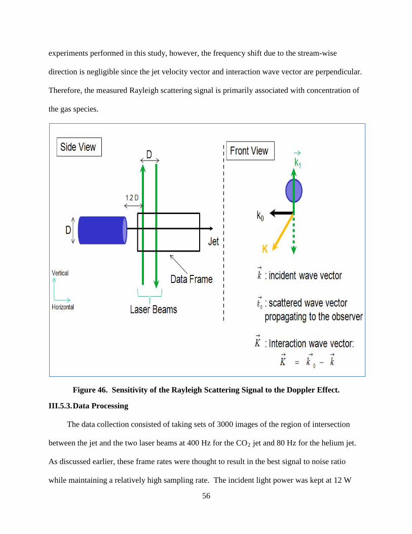
56

experiments performed in this study, however, the frequency shift due to the stream-wise

direction is negligible since the jet velocity vector and interaction wave vector are perpendicular.

Therefore, the measured Rayleigh scattering signal is primarily associated with concentration of

the gas species.

Figure 46. Sensitivity of the Rayleigh Scattering Signal to the Doppler Effect.

III.5.3. Data Processing

The data collection consisted of taking sets of 3000 images of the region of intersection

between the jet and the two laser beams at 400 Hz for the CO2 jet and 80 Hz for the helium jet.

As discussed earlier, these frame rates were thought to result in the best signal to noise ratio

while maintaining a relatively high sampling rate. The incident light power was kept at 12 W

57

during data collection. The camera was focused at the region of interest (intersection of the two

beams with the horizontal or curved jet). The image resolution was set at 1280x800 pixels for all

data measurements covering an area of interest of 59.5x37.5 mm as shown in Figure 47 below.

Some distortion can be seen on the edges of the frame in Figure 47 due to the use of the spherical

lens. However, the level of distortion in the area where the laser beams were was very small and

hence no correction was made during data processing. The bright regions of Figure 47

correspond to an intensity of 130 counts while the dark regions correspond to about 35 counts.

Figure 47. Unprocessed Image of Scattered Light of the Laser Going Through the CO2

For both the CO

Jet and Air at 400 Hz (Top) and the Grid Used for Spatial Reference (Bottom).

2

Figure 48

and helium configurations, essentially three different types of images

were collected to extract concentration information from the Rayleigh scattering signal. These

sets of data of which samples are shown in were the signal due to jet and air

molecules, signal due to air only, and background signal corresponding to collected images with

the laser turned off (or with the lens cap on).

58

Figure 48. Sample Images of Signals Used for Data Processing of Both the CO2 and Helium Configurations

For the purpose of the data processing, only the areas of intersection of the laser beams

with the jet were considered. Therefore, each frame was reduced to two matrices of dimensions

13x800 pixels. The width of 13 pixels corresponds to approximately 0.60 mm. The 16 bit

59

videos of the scattered light were initially converted to “Multipage. TIFF” format and then to

“.mat” using MATLAB. The raw intensity for any frame at any given imaging location was a

summation of the intensity due to Rayleigh scattering I, and the intensity of any captured

background light Io

The outcome of the initial post processing described above is the intensity I

. This latter term included reflections off test equipment such as the stainless

tubes used for this experiment or any lights in the laboratory. The background intensity was

corrected for and subtracted from the raw intensity. In addition, the electronic signal generated

by the camera was subtracted off from the scattered light signal. The electronic signal was

obtained by capturing images with the lens cap on.

R which is the

scattered light from both CO2 (and helium) and air molecules combined with background signal

subtracted. In order to convert the intensity IR to concentration of the jet only, the intensity IA of

air only was removed from the signal. IA was obtained by capturing images of the scattered light

of the ambient air only and subtraction of the electronic signal of the camera. The formula used

in this work to convert the intensity IR to CO2

concentration is given by:

where f is a correction factor that takes into account the ratio in cross section between air and

CO2 molecules. Typically, the Rayleigh scattering signal of the CO2 transmitted through the

filter is about twice the signal associated with air molecules. The ratio of the CO2 cross section

to the N2 cross section is about 2.23 while it is approximately 2.7 with respect to O2 25 [ ] which

yields the following relationship:

60

For this study; the correction factor f turns out to be about 2.45 to ensure 100% CO2

concentration at the core of the jet. IA is set to 28 intensity counts (and approximately 22 for the

case of the curved jet due to imaging through quartz) which correspond to the maximum value of

air intensity. Considering this peak intensity values into the equation allows for the use of a

more conservative calculation of the CO2

On the other hand, the formula used to convert the Rayleigh scattering signal intensity to

helium concentration is given by:

(or helium) jet concentration.

The Rayleigh scattering cross section ratio used in the formula above is 1.4 % as given by

Su et al. in their quantitative planar imaging of buoyant jet study [26].

Figure 49 and Figure 50 illustrate sample processed data for respectively the CO2 and

helium jets’ cases. For the case of CO2, brighter regions correspond to the Rayleigh scattering

signal due to CO2 Figure 49 molecules ( ) while signal due to helium molecules is associated with

areas of dimmer intensity (Figure 50). The concentration plots were created by averaging the

intensity values of all 3000 images for each pixel. The intensities were then converted to

concentrations using Equations (16) and (17) described above.

61

Figure 49. Raw Rayleigh Scattering Image (Left) and Processed Concentration Plot (Right) for the CO2 Configuration

Figure 50. Raw Rayleigh Scattering Image (Left) and Processed Concentration Plot (Right) for the Helium Configuration

In addition to concentration plots, concentration profiles were obtained by averaging the

concentration lines along the X/D (stream-wise) direction in a way to obtain a strip of

concentration running across the entire vertical direction as shown in Figure 51b. As part of the

analysis of the jet behavior, trajectory plots were also generated by tracking the maximum value

of the jet’s concentration along each strip located at every X/D location as shown in Figure 51c.

62

Figure 51. Sample CO2

In order to monitor the variation of the Rayleigh scattering intensity over time, standard

deviation of the signal’s raw intensity were generated using the std command of MATLAB.

These plots will be discussed in details in the Results and Analysis section of this report.

Process Data: (a) Percent Concentration, (b) Concentration Profile, (c) Jet’s Trajectory

In order to ensure the extraction of relevant and trust worthy information from the collected

data and analysis, it is important to approximate the overall percent error. There is obviously

instrumentation errors as specified when describing the equipment used for this research. The

equipment associated with the instrumentation errors include but are not limited to mass flow

controllers, traverse unit, laser power instability, thermocouples regulating the iodine filter

temperature, etc. All these errors could affect the end result which is the concentration of the jet.

In fact, this concentration depends on various parameters such as the incident power, the laser’s

wavelength, the position of the beam with respect to the jet, and others. The problem is that, for

this research, there is no direct equation that could relate all these parameters directly to the

concentration of the jet. Classical formulas of uncertainty cannot therefore be used in this case.

However, a repeatability analysis could be used to investigate the consistency of the information

a b

c

63

given by the collected signal. For that purpose, one case corresponding to a given flow condition

was run twice at two different times and results were compared. The standard deviation between

the jet concentrations of the two runs, when normalized by the mean, is considered to be an

approximation of the overall error of this analysis. Between the two presumably identical runs,

other cases were ran to allow for the manifestation of the inherent measuring errors such as the

change in the laser power over time, the drifting of the wavelength which affects the transmitted

light, the imperfection in the traverse unit setting and readout, etc. The case considered here was

one of the cases of the third experiment involving the investigation of G-loaded buoyant jet. It

was a case involving the presence of co-flowing air to take into account any errors due to the

vibration of the jet’s tube in the presence of co-flow. One stream-wise position was considered

which was an X/D of 1.3. Figure 52 illustrates the concentration profiles corresponding to the

1.3 D position from the first and second run.

Figure 52. Jet’s Concentration Profiles at 1.3 D

64

Figure 53. Position one (X/D=1.3): (a) Standard Deviation and (b) Mean

As shown in Figure 52, the two runs are very close to each other. It is however hard to

quantify the difference between them. For that purpose, Figure 53 was generated to estimate the

error between the two runs based on the standard deviation. At this position (X/D = 1.3), the

standard deviation in the area of the core of the jet is approximately 3 % while the mean has a

maximum value of 98%. This results in an error of approximately 3 % in the core of the jet

which is the interest of this study mainly when tracking the trajectory of the jet. The error in the

areas around the core of the jet is higher than at the core. In addition, the errors increase as the

stream-wise location increases due to the weakening of the signal as a result of mixing and due

to the slight difference power of the two laser beams off of which the Rayleigh scattering signal

is collected.

Every time, a laser beam hits the surface of a mirror or a prism it loses a small percentage

of its power. The second laser beam is created off of the first beam through the use of a prism.

65

In order to quantify the difference in power between the two laser lines, the Rayleigh scattering

signal due to the presence of air only collected off of both laser beams was considered.

Figure 54. Rayleigh-Scattering Signal Due to Air Associated with the First and Second Laser Beams: (a) Raw Images and (b) Intensity Counts

A raw images of the two signals is shown in Figure 54a. Figure 54b illustrates the intensity

counts of the two Rayleigh scattering signals due to air. Based on the ratio of the average

intensity values of the two signals, the second line has approximately 97.5 % power of the first

line. This difference was taken into account when generating the concentration data. When

processing the data for this research the information corresponding to the first line was chosen in

favor of the one (in most cases) associated with the second line every time there was an overlap

between the two lines. The laser beam comparison leads to adding a 2.5 % possible error to the

4% error found above.

66

IV. Results and Analysis

IV.1. Experiment # 1 : Iodine Filter Characterization

The data obtained for iodine filter characterization is transferred to an EXCEL sheet and

transformed into graphs to be laid out and discussed in this section. Multiple runs were

performed in order to validate the consistency of both the filter’s behavior and the data

acquisition method. For the iodine cell temperature set at 90 o C and 40 o

Figure 55

C, two tests were

performed for each temperature. and Figure 56 below illustrate the findings of this step

and show negligible variation of the results when comparing the two tests.

Figure 55. Repeatability Test of the Transmitted Power of the Filter at 90 o

C

0

10

20

30

40

50

60

70

80

18787.76 18787.78 18787.8 18787.82 18787.84 18787.86 18787.88

Tran

smit

ted

Pow

er (%

)

Wavenumber (cm-1)

Run # 1 (90 deg C)

Run # 2(90 deg C)

67

Figure 56. Repeatability Test of the Transmitted Power of the Filter at 40 o

The optimal iodine cell temperature corresponds to the temperature at which the frequency

range corresponding to transmission is the largest. Operating the cell temperature at the optimal

temperature ensures maximum blocking of the unwanted background signal. Based on

C

Figure 57

below, among the three tested temperatures, 90 o C appears to be the optimal temperature for the

iodine molecular filter in use. In addition, the absorption well depth increases as the temperature

increases. Therefore, for future uses of the iodine filter (the second and third experiment), the

cell temperature will be set at 90 o C.

0

10

20

30

40

50

60

70

80

90

18787.76 18787.78 18787.8 18787.82 18787.84 18787.86

Tran

smit

ted

Pow

er (%

)

Wavenumber (cm-1)

Run # 1 (40 deg C)

Run # 2 (40 deg C)

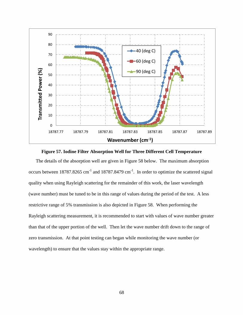
68

Figure 57. Iodine Filter Absorption Well for Three Different Cell Temperature

The details of the absorption well are given in Figure 58 below. The maximum absorption

occurs between 18787.8265 cm-1 and 18787.8479 cm-1

Figure 58

. In order to optimize the scattered signal

quality when using Rayleigh scattering for the remainder of this work, the laser wavelength

(wave number) must be tuned to be in this range of values during the period of the test. A less

restrictive range of 5% transmission is also depicted in . When performing the

Rayleigh scattering measurement, it is recommended to start with values of wave number greater

than that of the upper portion of the well. Then let the wave number drift down to the range of

zero transmission. At that point testing can began while monitoring the wave number (or

wavelength) to ensure that the values stay within the appropriate range.

0

10

20

30

40

50

60

70

80

90

18787.77 18787.79 18787.81 18787.83 18787.85 18787.87 18787.89

Tran

smit

ted

Pow

er (%

)

Wavenumber (cm-1)

40 (deg C)

60 (deg C)

90 (deg C)

69

Figure 58. Iodine Filter Absorption Well at 90o

Based on the literature, the absorption well can be expressed also as a function of the

wavelength (in nm) or a relative frequency (in GHz). The relative frequency is calculated by

taking the difference with respect to a reference frequency that corresponds to the center of the

well. In order to be able to compare the results with previous filter’s characterization in the

literature, three more graphs

C

Figure 59 , Figure 60 , and Figure 61 were also generated. The

center of the well corresponds to a wavelength of 532.1099054 nm in air, a wavelength of

532.2580152 nm in vacuum, and a reference frequency of 563245.1895 GHz.

70

Figure 59. Iodine Filter Absorption Well with Respect to Wavelength in Air

Figure 60. Iodine Filter Absorption Well with Respect to Wavelength in Vacuum

0

10

20

30

40

50

60

70

80

532.108 532.1085 532.109 532.1095 532.11 532.1105 532.111

Tran

smit

ted

Pow

er (%

)

Wavelength in air (nm)

90 (deg C)

0

10

20

30

40

50

60

70

80

532.256 532.2565 532.257 532.2575 532.258 532.2585 532.259 532.2595

Tran

smit

ted

Pow

er (%

)

Wavelength in vaccum (nm)

90 (deg C)

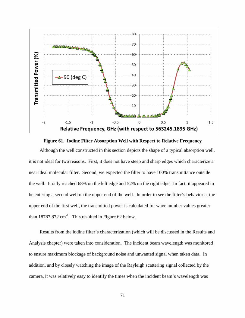
71

Figure 61. Iodine Filter Absorption Well with Respect to Relative Frequency

Although the well constructed in this section depicts the shape of a typical absorption well,

it is not ideal for two reasons. First, it does not have steep and sharp edges which characterize a

near ideal molecular filter. Second, we expected the filter to have 100% transmittance outside

the well. It only reached 68% on the left edge and 52% on the right edge. In fact, it appeared to

be entering a second well on the upper end of the well. In order to see the filter’s behavior at the

upper end of the first well, the transmitted power is calculated for wave number values greater

than 18787.872 cm-1 Figure 62. This resulted in below.

Results from the iodine filter’s characterization (which will be discussed in the Results and

Analysis chapter) were taken into consideration. The incident beam wavelength was monitored

to ensure maximum blockage of background noise and unwanted signal when taken data. In

addition, and by closely watching the image of the Rayleigh scattering signal collected by the

camera, it was relatively easy to identify the times when the incident beam’s wavelength was

0

10

20

30

40

50

60

70

80

-2 -1.5 -1 -0.5 0 0.5 1 1.5

Tran

smit

ted

Pow

er (%

)

Relative Frequency, GHz (with respect to 563245.1895 GHz)

90 (deg C)

72

within the range of the filter’s absorption well. Figure 63 illustrates the difference between the

transmitted Rayleigh scattering signal when inside and outside the filter’s absorption well.

Figure 62. Investigation of the Upper End on the Absorption Well

Figure 63. Rayleigh-Scattering Signal Inside and Outside the Filter’s Absorption Well

0

10

20

30

40

50

60

70

80

18787.77 18787.79 18787.81 18787.83 18787.85 18787.87 18787.89 18787.91

Tran

smit

ted

Pow

er (%

)

Wavenumber (cm-1)

90 (deg C)

Unwanted Background Scattering Light

Rayleigh-Scattering Imaging Lines

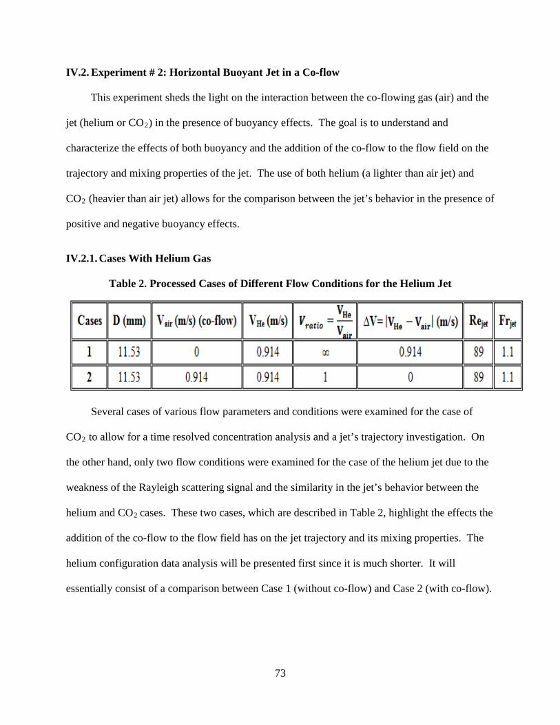
73

IV.2. Experiment # 2: Horizontal Buoyant Jet in a Co-flow

This experiment sheds the light on the interaction between the co-flowing gas (air) and the

jet (helium or CO2) in the presence of buoyancy effects. The goal is to understand and

characterize the effects of both buoyancy and the addition of the co-flow to the flow field on the

trajectory and mixing properties of the jet. The use of both helium (a lighter than air jet) and

CO2

IV.2.1. Cases With Helium Gas

(heavier than air jet) allows for the comparison between the jet’s behavior in the presence of

positive and negative buoyancy effects.

Table 2. Processed Cases of Different Flow Conditions for the Helium Jet

Several cases of various flow parameters and conditions were examined for the case of

CO2 to allow for a time resolved concentration analysis and a jet’s trajectory investigation. On

the other hand, only two flow conditions were examined for the case of the helium jet due to the

weakness of the Rayleigh scattering signal and the similarity in the jet’s behavior between the

helium and CO2 cases. These two cases, which are described in Table 2, highlight the effects the

addition of the co-flow to the flow field has on the jet trajectory and its mixing properties. The

helium configuration data analysis will be presented first since it is much shorter. It will

essentially consist of a comparison between Case 1 (without co-flow) and Case 2 (with co-flow).

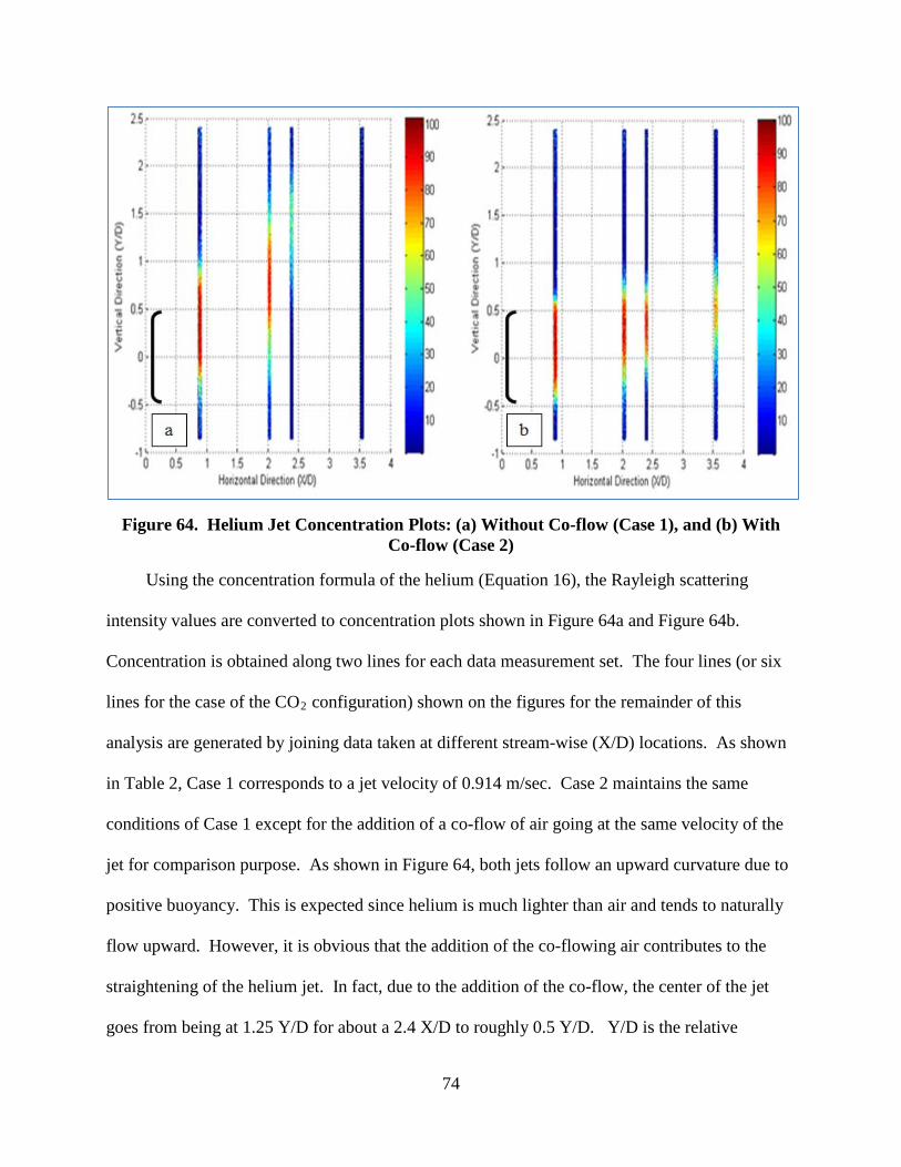
74

Figure 64. Helium Jet Concentration Plots: (a) Without Co-flow (Case 1), and (b) With Co-flow (Case 2)

Using the concentration formula of the helium (Equation 16), the Rayleigh scattering

intensity values are converted to concentration plots shown in Figure 64a and Figure 64b.

Concentration is obtained along two lines for each data measurement set. The four lines (or six

lines for the case of the CO2

Table 2

configuration) shown on the figures for the remainder of this

analysis are generated by joining data taken at different stream-wise (X/D) locations. As shown

in , Case 1 corresponds to a jet velocity of 0.914 m/sec. Case 2 maintains the same

conditions of Case 1 except for the addition of a co-flow of air going at the same velocity of the

jet for comparison purpose. As shown in Figure 64, both jets follow an upward curvature due to

positive buoyancy. This is expected since helium is much lighter than air and tends to naturally

flow upward. However, it is obvious that the addition of the co-flowing air contributes to the

straightening of the helium jet. In fact, due to the addition of the co-flow, the center of the jet

goes from being at 1.25 Y/D for about a 2.4 X/D to roughly 0.5 Y/D. Y/D is the relative

75

normalized vertical location of the jet with respect to the center of exit of the tube while X/D is

the normalized horizontal (stream-wise) location of the jet measured from the exit of the tube.

As far as the mixing of the jet with air, it seems that the diffusion of the helium into air, at the

same X/D location, is more significant in the absence of the co-flow. However, for both cases

the mixing and the level of turbulence of the jet increases downstream of the jet as shown in

Figure 65 of the standard deviation plots.

Figure 65. Standard Deviation of Helium Intensity: (a) Without Co-flow (Case 1) and (b) With Co-flow (Case 2)

For both cases (Figure 65a and Figure 65b), the mixing occurs initially in the top and

bottom shear layers of the regions of interaction between the jet and the co-flowing air. As the

jet moves downstream, it loses a lot of its momentum and the mixing moves progressively

toward the center of the jet as shown in both Figure 65a and Figure 65b. It is important to note

76

as well that for Case 2 (with co-flow), the top shear layer is much more significant than the

bottom shear layer due to the tendency of the jet to go up (positive buoyancy) which is expected.

The observations noted based on Figure 64 and Figure 65 can also be extracted by simply

examining the concentration profile plots of Figure 66.

Figure 66. Helium Concentration Profiles: (a) Without Co-flow (Case 1) and (b) With Co-flow (Case 2)

Clearly, the addition of the co-flow straightens the trajectory of the helium jet which

maintains its overall upward curvature due to positive buoyancy effects. In addition, the profiles

(in both cases) get wider as the stream-wise location increases due to the diffusion of the jet into

air. The straightening and flattening of the jet can also be seen in the trajectory plots of Figure

67. The idea here is to track the approximate position of the center of the jet by identifying the

location of the maximum value of concentration.

77

Figure 67. Helium Jet Trajectory With Co-flow (Case 1) and Without co-flow (Case 2)

The work of Reeder et al., mentioned earlier in the literature review section, provides jet

core trajectory data that could be checked against the findings of this study. The horizontal and

vertical locations have to be, however, normalized by a length scale for “the transition of a

horizontal buoyant jet to a plume” LM 18 defined by the authors as follows [ ]:

The velocity of the jet is Vjet, A is the cross sectional area of the jet, g is the gravitational

constant; ρair and ρjet are respectively air and jet densities. The value of LM

Table 2

for Case 1 is

calculated to be 12.0 mm. As shown in , Case 1 corresponds to a Froude number of 1.1.

Case 1 trajectory points are then plotted against a case from Reeder et al. study with a value of

Froude number of 1.14 as shown in Figure 68. Reeder et al. used a weighted averaged method to

generate the trajectory data points shown in Figure 68. Despite the fact that the two studies used

78

different methods to track the trajectory of the jet, the two curves are in a very strong agreement.

This comparison indicates that that tracking the jet using the maximum value of concentration

for each stream-wise profile is a valid approach.

Figure 68. Comparing Case 1 of the Helium Configuration Trajectory Points to the Literature

IV.2.2. Cases With CO2

Various cases were run to construct sufficient data to allow for the qualitative investigation

of both the trajectory behavior and mixing properties of the CO

Gas

2 jet as a function of different

parameters. These parameters include the velocity of air (the co-flow velocity), the CO2

jet

velocity, the relative velocity of the jet with respect to the co-flow, the velocity ratio, Reynolds

number, and Froude number. These cases are illustrated in Table 3.

79

Table 3. Processed Cases of Different Flow Conditions for the CO2

Jet

Figure 69a and Figure 69b show the mean concentration for series of 3000 images taken for

two different cases. The six separate vertical lines in each plot correspond to three separate runs

as two lines are imaged in each time sequence. Case 1(shown in Figure 69a) represents a typical

jet flow, with a jet velocity of 0.305 m/sec and no co-flow configuration. Case 2, however,

shown in Figure 69b differs from Case 1 (Figure 69a) by the addition of a co-flow of air going at

the same speed as the CO2 jet of Case 1. As expected, the heavier than air jet is subject to a

negative buoyancy effects resulting in the CO2 concentration locations following a curved down

trajectory in both cases.

80

Figure 69. CO2

Significant changes occur to the flow structure and behavior when a co-flow of air is

introduced as seen in Case 2 concentration and standard deviation plots. First, the trajectory

becomes flatter as noticed when comparing

Jet Concentration Plots: (a) Without Co-flow (Case 1), and (b) With Co-flow (Case 2)

Figure 69a and Figure 69b. The concentration of the

CO2

Figure 70

drops to less than 10% at X/D = 4.4 as opposed to 65% at the core of the jet in the Case of

no co-flow. Furthermore, stronger regions of mixing (as seen in b) are developed even

at closer locations away from the exit of the jet (X/D = 1.2). For both Case 1 and Case 2, the

increase in mixing is more pronounced with downstream distance. As shown in Figure 70b, for

instance, starting from a jet location of X/D = 3.2, the fluctuation of the jet intensity

(concentration) becomes more significant especially along the shear layers on the top and bottom

of the core of the jet. At 4.4 D, the region of the center of the jet was subject to the strongest

fluctuations indicating mixture of the center of the jet with ambient air. As expected, the level of

fluctuation is more significant in the bottom shear layer than on the top due to the uneven density

distribution resulting from the existing negative buoyancy. The mixing of the jet with the co-

81

flowing air moves progressively from the top and bottom shear layers to the core of the jet. This

entrainment results in the significant decrease of the CO2

concentration as the jet travels

downstream.

Figure 70. Standard Deviation of CO2

Intensity: (a) Without Co-flow (Case 1) and (b) With Co-flow (Case 2)

Figure 71. CO2 Concentration Profiles: (a) Without Co-flow (Case 1) and (b) With Co-flow (Case 2)

82

The changes in the jet behavior the addition of the co-flow causes are also highlighted in

Figure 71. The flattening of the jet trajectory can be noticed by comparing the profiles of Case 1

(Figure 71a) to that of Case 2 (Figure 71b). In addition, the figures indicate a decrease in the

CO2 concentration with downstream distance from the exit of the jet for both with and without

co-flow. Furthermore, there is an overall spreading of the jet due to the mixing of the CO2 with

the ambient air. Unlike the cases with the helium jet, the co-flow in the case of the CO2

jet

seems to increase the mixing of the jet and its diffusion into air.

Figure 72. Comparing Jet Trajectory for no Co-flow Cases (1, 3 and 5) and With Co-flow Cases (2, 4, and 6)

As part of the analysis of the jet behavior, trajectory plots were also generated. Figure 72

compares the trajectory of CO2 jets at Froude numbers of 1.73, 2.6, and 3.45 for conditions with

83

and without a co-flow of 0.305 m/s. Readily apparent is that the addition of the co-flow

significantly flattened the trajectory of the jet. For example when the co-flow is added, such as

in Case 2, the trajectory curvature decreased and the jet dropped with only a vertical position of

Y/D= -0.5 as opposed to approximately -1.5 for Case 1. Although they had the same jet velocity

(0.305 m/sec), the two cases had different trajectory pattern which indicates the need to alter the

classical definition of Froude number (Equation 8) to incorporate the effects of co-flow on the

buoyancy of the jet and its trajectory. In addition, for a velocity ratio of 2.0 (Case 6), the jet has

greater momentum than Case 2 (velocity ratio of 1.0) and Case 4 (velocity ratio of 1.5) and

hence exhibits a smaller overall vertical drop of 0.40 D at X/D = 3.5 as opposed to 0.60 D for

Case 2. Similar investigation was performed by comparing cases 1, 3, and 5. The co-flow

velocity for these cases however was kept at 0 m/sec while the jet velocity varied from 0.305

m/sec (Case 1) to 0.458 m/sec (Case 3) to 0.610 m/sec (Case 5). As shown in Figure 72, the

effect of buoyancy (curving the trajectory) is more pronounced in the absence of the co-flow. In

addition, the higher the jet velocity, the smaller the overall drop of the jet at 4.4 D. Cases 3 and

5 have close values of Froude number (2.6 and 3.45) which explains the similarity between their

respective trajectories. This indicates that in the absence of the co-flow, the classical definition

of the Froude number holds true. Overall, for both the co-flow and no co-flow cases, the

trajectory is less curved as the jet velocity (and thus the Froude number) increases.

Case 1 core jet trajectory, which corresponds to a Froude number of 1.73, can be compared

against a comparable case from the literature with Froude number of 1.8. The length scale for

Case 1 is found to be about 14.50 mm. Figure 73 below illustrates this comparison which

indicates a relatively close agreement between the two studies.

84

Figure 73. Comparing Case 1 of the CO2

The data presented up to this point with the exception of the standard deviation plots is

time averaged data that does not reflect the time resolved aspect of this study. Hence,

highlighting the behavior of the jet as a function of time is the objective of this section. As

shown in

Configuration Trajectory Points to the Literature

Figure 70, the addition of the co-flow to the flow fields causes the unsteadiness of the

jet concentration that increases as the stream-wise location (X/D) increases. In order to convey

this unsteadiness seen in the collected images of Case 1 (without the co-flow), and Case 2 (with

co-flow), Figure 74 is generated. It illustrates a comparison between these two cases using four

images of each case taken at four different instants in time. While the jet remains relatively

steady over time in the absence of the co-flowing air, it exhibits significant unsteadiness when air

is added to the flow field.

85

Figure 74. CO2

The significant changes introduced by the addition of the co-flow prompts the investigation

of time resolved data of the mixing regions.

Raw Data Images With Co-flow (Case 2) and Without Co-flow (Case 1)

Figure 75a and Figure 75b illustrate the two

dimensional standard deviation plots for Case 1 and Case 2 respectively. As shown in Figure

75a, minimal mixing occurs at 1.2 D away from the exit of the jet with a small increase of the

level of fluctuations in the top and bottom shear layers. Case 2, however, exhibits significant

fluctuations level at the shear layers and was therefore used as a baseline for time histories

analysis. The standard deviation plot of Case 2 at X/D = 1.2 D is shown in Figure 75b.

86

Figure 75. Two Dimensional Standard Deviation Plots of: (a) Case 1 (Vjet = 0.305 m/sec, V-co-flow = 0 m/sec), (b) Case 2 (Vjet = 0.305 m/sec, Vco-flow

Four points of interest were then chosen based on the plot of the standard deviation (as

shown in

= 0.305 m/sec), and (c) Comparison of Case 1 and Case 2

Figure 75b). Time histories of points 1, 2, 3, and 4 are plotted together in Figure 76.

Points 1, 3, and 4 correspond to peaks in the fluctuations due to the top and bottom of the shear

layer regions. Point 2 corresponds to a point of low standard deviation which is relatively away

from the shear layer and close to the core of the jet where less mixing occurs (at that X/D

location). Note that the intensity counts indicated in Figure 76 and Figure 77 are much higher

than those shown in previous standard deviation plots. This is because nine pixels are binned

together for each point location to minimize noise and obtain cleaner time history plots. As

evident from these time histories, the fluctuations in the upper and lower shear layer are regular

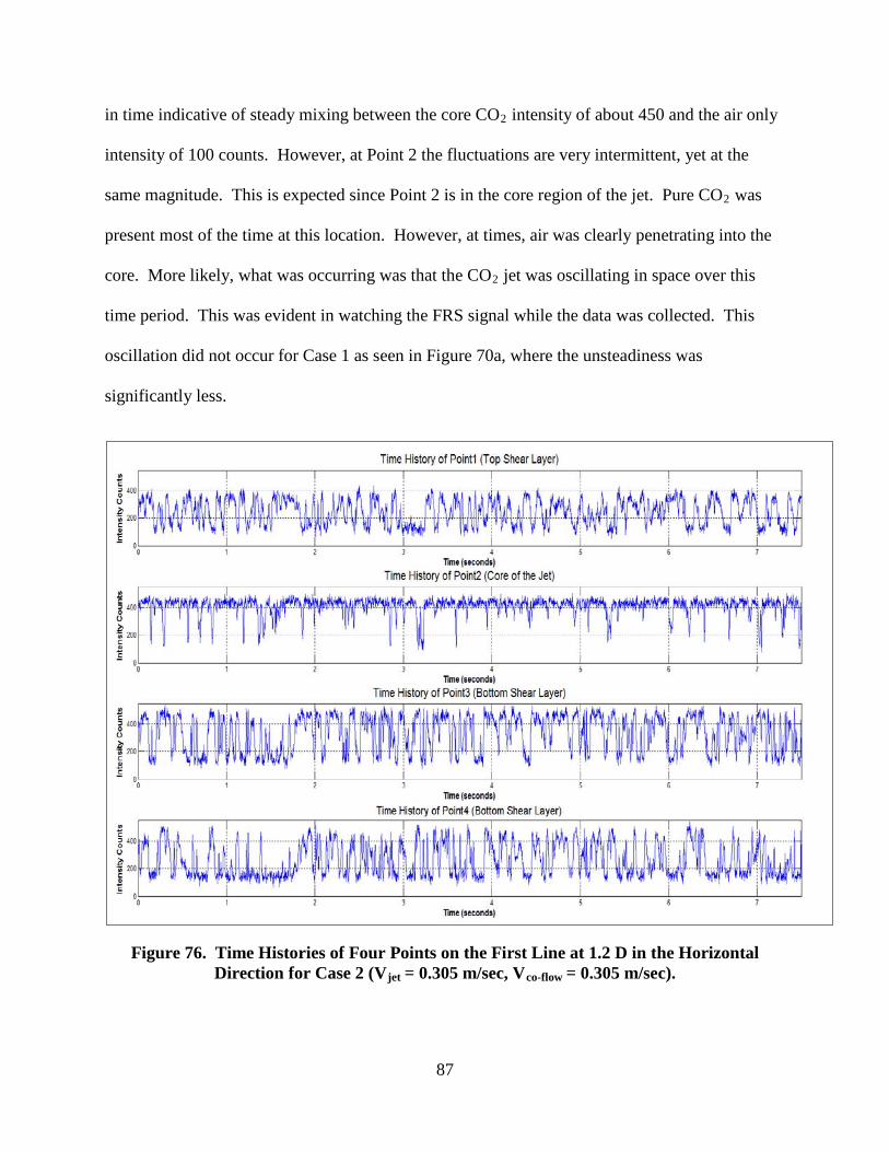
87

in time indicative of steady mixing between the core CO2 intensity of about 450 and the air only

intensity of 100 counts. However, at Point 2 the fluctuations are very intermittent, yet at the

same magnitude. This is expected since Point 2 is in the core region of the jet. Pure CO2 was

present most of the time at this location. However, at times, air was clearly penetrating into the

core. More likely, what was occurring was that the CO2

Figure 70

jet was oscillating in space over this

time period. This was evident in watching the FRS signal while the data was collected. This

oscillation did not occur for Case 1 as seen in a, where the unsteadiness was

significantly less.

Figure 76. Time Histories of Four Points on the First Line at 1.2 D in the Horizontal Direction for Case 2 (Vjet = 0.305 m/sec, Vco-flow = 0.305 m/sec).

88

Figure 77. Time Histories of Points 3 and Point 4 of Case 2 (Vjet = 0.305 m/sec, Vco-flow

= 0.305 m/sec).

Figure 78. Cross-Correlation of Point 4 to Point 3 of Case 2 (Vjet = 0.305 m/sec, Vco-flow = 0 m/sec)

0.17 St = 0.17

89

Figure 77 was generated in light of what appeared to be a time lag between Point 3 and

Point 4 time histories given in Figure 76. These two points were located in the area of high

fluctuations in the lower shear layer, as shown in Figure 75b. As indicated above, the two points

have the same X/D location (1.206 D) and are offset by a vertical distance of 0.13 D or 1.15 mm.

From the cross correlation plot (shown in Figure 78), there exists a small time lag (less than

0.0025 seconds) between the time histories of the data taken from the two locations. The

magnitude of the lag indicates a correlating velocity of 0.46 m/sec between the two points; while

the high correlation between Point 3 and Point 4 was indicative of that the structure of the

vortices was regular and coherent. Furthermore, the secondary peaks in the cross correlation

(shown in Figure 78) suggest the presence of a repeating pattern every 0.17 seconds (5.9 Hz)

which could be associated with the shedding frequency of the flow structure. This frequency

corresponded to a Strouhal number (St) of 0.173. The Reynolds number is 339 for this case

which corresponded to a Strouhal number of 0.20 for a flow around a cylinder traveling at a

comparable speed to that of Case 2. This compares favorably with the work of Baranyi et al.

27[ ].

In addition, it is often useful when time resolved data is collected to perform a Fast Fourier

Transform (FFT) on the time dependent information to identify the frequency content of the

signal. An FFT is then performed on a 20 second long time history of Point 3 of Case 2 as

indicated above. The frequency spectrum of the signal, shown in Figure 79, indicates the

presence of a frequency at 6 Hz which could correspond to the same frequency (5.9 Hz)

identified through the correlation plots.

90

Figure 79. Frequency Content of 20 Second Long Time History of Point 3 of Case 2

Figure 80. Two Lines Cross- Correlation for Case 7 (Vjet = 0.153 m/sec, Vco-flow = 0.153 m/sec)

91

Figure 81. Two Lines Cross- Correlation for Case 2 (Vjet = 0.305 m/sec, Vco-flow

= 0.305 m/sec)

Figure 82. Two Lines Cross- Correlation for Case 8 (Vjet = 0.610 m/sec, Vco-flow = 0.610 m/sec)

92

Figure 80, Figure 81, and Figure 82 show cross-correlation plots between a point on the

first line (at 1.2 D away from the exit of the jet) and a point on the second line (at 2.4 D away

from the exit of the jet) for cases 7, 2, and 8 respectively. Standard settings for the xcorr routine

in MATLAB were applied, and as a result, the values on the vertical axis should not be

compared from one plot to another, as they are affected by the standard deviation for each point.

Nonetheless, the peak corresponding to a lag time for a given plot may be used to characterize

events in the flow field. The ratio of the jet velocity to the co-flow velocity was maintained at 1.0

for all three cases. For cases 7, 2, and 8, the jet velocities are respectively 0.153 m/sec, 0.305

m/sec, and 0.610 m/sec. These cases enable correlation plots to deduce the mean convective

velocities of flow features within the jet. Figure 80, Figure 81, and Figure 82 indicate the

presence of a significant lag of 0.0475 sec, 0.02 sec, and 0.0125 sec respectively between points

of the first line and points of the second line which is expected. As shown in Figure 80, the

chosen point on the second line is not on the same height as the point on the first line due to the

drop of the jet trajectory. This vertical drop due to buoyancy increased the distance the jet

traveled between the first and second point and hence added to the time lag. The corresponding

convective velocities given the horizontal distances between the points of the first line and those

of the second line are respectively 0.225 m/s, 0.536m/s, and 0.858 m/s. These values are higher

than the actual jet velocities of cases 7, 2, and 8. This significant difference between the

calculated and expected convective velocities can be due in part to the fact that the flow exiting

the tube is unlikely to have a top hat profile but, rather, would have velocities higher than the

nominal values listed in Table 3 in the core of the jet. On the other hand, as the jet velocity

increased proportionally with the mass flow controller setting, the correlation peaks shifts to a

smaller time lag, which is an expected trend. In other words, the shift in the time lag is inversely

93

proportional to the increase in the jet velocity, demonstrating the value of the measurement

technique.

The second portion of the data analysis involves investigating the effects of the parameters

discussed previously on the jet trajectory. In Figure 83, the relative velocity was kept constant at

0.305 m/sec while the velocity of the jet was changed. The jet velocity for Case 9 was three

times that of Case 1 and one and a half that of Case 6 which corresponded to a Froude increase

from 1.73 to 3.45 to 5.18. Readily apparent was that the trajectory was straighter for the higher

Froude number jet (i.e. higher velocity). This highlights the importance of the jet velocity in

shaping the trajectory. This also suggests that the relative velocity between the jet and core flow

is not the proper scaling velocity for buoyant flows.

Figure 83. Effects of Jet Velocity on the Jet’s Trajectory

94

Figure 84. Effects of Froude Number on the Jet’s Trajectory

A set of runs were performed while maintaining the Froude number constant. To

accomplish this, three different combinations of jet diameter were used. Cases 8, 10 and 11

shown in Figure 84, corresponded respectively to Reynolds number values of 678, 992, and

1800. It might be expected that Case 11, with a Reynolds number of 1800, would have a

relatively higher trajectory than the other two cases. However, all these cases corresponded to a

Froude number of 3.45 based on jet velocity and diameter (based on the classical definition of

the Froude number of Equation (8)). As indicated in Figure 84, all three of these cases

maintained a tight distribution suggesting that the Froude number has a substantial impact on the

trajectory. One note is that these three cases all maintained a constant co-flow velocity of 0.610

m/s. To look specifically at the effect of the co-flow, Case 5, which corresponds to Case 8

without the co-flow, was also plotted. The curvature of the trajectory was more pronounced in

Case 5. This reemphasized that the presence of the co-flow impacts the overall structure of the

jet, including the turbulence, as well as altering the buoyancy. However, it does not appear that

95

once the turbulence is increased, that any further increases in the co-flow velocity has any further

effect.

Figure 85. Effects of Relative Velocity on the Jet’s Trajectory (Maintaining Fr = 3.45)

In order to further investigate the impact of the relative velocity on the jet’s trajectory,

Cases 5 and 6 were further compared to Case 8. These three configurations corresponded to a

Froude number of 3.45 based on the classical definition of Froude number outlined in Equation

(8). The co-flow velocity was changed from 0 (Case 5) to 0.305 m/sec (Case 6) to 0.610 m/sec

(Case 8). This resulted in a substantial change in the velocity ratio and the relative velocity

between the jet and the co-flow. As shown in Figure 85, Cases 6 and 8 trajectories were similar.

This indicates that the relative velocity parameter had a minimal effect on the jet trajectory. It

also emphasizes the significant change that occurred when the co-flow was added. The addition

of the co-flow to the flow field seems to have the effect of increasing the turbulence and thus the

96

spreading rate of the jet. Once this turbulence is activated, a further increase in the co-flow

velocity is not significant.

To better understand the impact of velocity ratio on the jet’s trajectory, Cases 6, 12, and 13

were further compared. Each of these cases maintained velocity ratio of 2.0 between the jet and

the co-flow. Both the jet velocity and the co-flow were increased between these cases. This

resulted in an increase in the relative velocity and Froude number. For the highest value of

Froude number (Case 13), the trajectory of the jet is almost linear as shown in Figure 86a. The

velocity ratio between the two flows was clearly not the normalizing factor as changing the

relative velocity altered the impact of the buoyancy. For these conditions, the relative velocity

was increased by a factor of 2 (from Case 6 to Case 12) and by a factor of 3 (from Case 6 to Case

13). To remove influence of the relative velocity, four other cases were interrogated. These

cases maintained the velocity ratio at 1.0 while also maintaining the relative velocity constant at

0. Figure 86b reveals still a significant variation in the trajectory of these jets indicative that the

buoyancy still has a dominant effect. This effect is not attributed to either the velocity ratio or

the relative velocity between the jet and co-flow. What did change significantly for these cases

was the Froude number which took on the values of 0.75 (Case 7), 1.73 (Case 2), 3.45 (Case 8),

and 7 (Case 14). Clearly for these cases, the higher the Froude numbers (and hence the jet

trajectory) the straighter the trajectory of jet was. This clearly indicates that the jet velocity itself

has stronger impact on the buoyancy than the co-flow velocity.

97

Figure 86. Effects of Velocity Ratio on the Jet’s Trajectory: (a) Vratio = 2.0 , (b) Vratio

= 1.0

Figure 87. Effects of Reynolds Number on the Trajectory

To validate this, the Reynolds number was investigated in Cases 15, 16, and 17. Figure 87

presents a comparison of the jet trajectory at a constant Reynolds number of 1430 while the

98

Froude number is respectively 2.75, 4.97, and 7.3. This was accomplished by varying the jet

diameter and the jet velocity systematically. The respective trajectories were nearly flat for these

cases. This highlights that the buoyancy is dictated by characteristics of the jet such as the jet’s

velocity and diameter. This in turns validates the dependence of the jet trajectory on the Froude

number (which depends on the jet’s characteristics). However, as mentioned above, the effect of

the co-flow in straightening the overall trajectory of the jet cannot be ignored and has to be

incorporated in the formula of the Froude number.

IV.3. Experiment # 3: G-loaded Buoyant Jet in a Co-flow

Various cases were run and processed to investigate the effect of G-loading on the

trajectory and mixing behavior of the jet. As shown in Table 4 cases of high (up to 1500) and

low G-loading (as low as 0.07) were considered.

Table 4. G-loaded Buoyant Jet Cases

99

Earlier analysis on the horizontal buoyant jet indicated that the co-flow contributed in

straightening the jet trajectory and increasing the mixing of the jet with air. Plots of the jet’s

raw intensity counts or percent standard deviation are usually employed to highlight areas of

mixing and changes of the jet’s concentration. However, for the G-loaded jet’s experiment, the

laser beams went through windows of quartz through which imaging occurred. This

significantly lowered the overall collected intensity of the Rayleigh scattering signal causing a

lower difference between the intensity counts in the core of the jet and in the top and bottom

shear layer. Changes in the fluctuations of the jet could not then be picked up by the standard

deviations and hence standard deviation plots were not generated for this section. Another

reason for which the standard deviation plots were not useful in this case was that at high G-

loading, the velocity of the jet was so fast to the point the changes due to mixing were not picked

up. To illustrate this observation, three points, as shown in Figure 88, were considered on the

first position line (X/D = 1.33 D) of Case 11 where some fluctuations were noted by visually

inspecting the collected images. Point 1 is located in the top shear layer, Point 2 is in the middle

of the jet, and Point 3 is in the bottom shear layer.

Figure 88. Locations of the three Considered Points of Case 5 (G-loaded Jet)

100

Figure 89. Time Histories of the Three Points of Figure 88

As indicated in Figure 89, the standard deviations of the Rayleigh scattering signal

intensity of the three points had similar values around 20 counts. There were no significant

changes in the standard deviation going from the top shear layer, to the core of the jet, and to the

bottom shear layer. Based on the collected video (and images) for this case, the signal to noise

ratio was very low. For cases 1 through 5, the velocity of the jet was comparable to cases run in

the horizontal jet experiment where standard deviation plots exhibited relatively higher values.

The signal to noise ratio, for the case of the G-loaded jet however, was much lower due to the

fact that imaging now occurs through quartz (which was not the case for the case of the

horizontal jet experiment). This explains the irrelevance of plotting the standard deviation of

which a sample plot is provided in Figure 90.

101

Figure 90. Case 11 Standard Deviation (Intensity Counts) Plot

Initially, when processing the data, the intent was to plot the concentration data of the jet at

six different stream-wise locations. However, due to the inconsistency in the laser power and

possible (unnoticed) minor drifts of the laser’s wavelength over time, the concentration lines

which correspond to the third position (after the traverse was moved two diameters) for cases 1

through 10 and 17 were ignored. In addition, the lines corresponding to second position (after

the traverse was moved one diameter) for cases 11 through 16 and 18 were also ignored for the

same reason.

Part of the analysis in this section involves understanding the effects of the addition of the

co-flow to the flow field on the jet’s behavior in the presence of G-loading. Figure 91, Figure

92, Figure 93, and Figure 94 illustrate concentration plots of the CO2 jet when it is subject to

respectively a G-load of 0.07, 4,100, and 1000.

102

Figure 91. CO2 Jet Concentration Plots for Gjet

= 0.07: (a) Case 1 (With Co-flow) and (b) Case 2 (Without Co-flow)

Figure 92. CO2 Jet Concentration Plots for Gjet

= 4: (a) Case 9 (With Co-flow) and (b) Case 10 (Without Co-flow)

103

Figure 93. CO2 Jet Concentration Plots for Gjet

= 100: (a) Case 11 (With Co-flow) and (b) Case 12 (Without Co-flow)

Figure 94. CO2 Jet Concentration Plots for Gjet = 1000: (a) Case 15 (With Co-flow) and (b) Case 16 (Without Co-flow)

104

With the exception of Case 1 and Case 2 where the G-loading and the jet velocities were

small, it was very apparent that the co-flow contributed to increasing the mixing of the jet with

air. This could clearly be seen especially when comparing the jet concentration with and without

co-flow for the cases considered in figures above. In fact, the plots illustrated more spreading of

the jet across the vertical location in the presence of the co-flow which indicated the occurrence

of more mixing. It was not apparent however, at low G-loading values that the increase in the G-

loads contributed to a significant change in the mixing of the jet. Concentration profiles of cases

corresponding to different G-loading were then generated to investigate the effect of G-loading

on the jet trajectory and the structure of the jet. At relatively low G-loading (between 0.07 and

4), the G-loading does not seem to drastically influence the direction of the jet nor its core

structure. This observation is underlined when looking at the jet concentration profiles at G-

loadings of 0.07, 1,2,3 and 4 with and without co-flow as shown in Figure 95, Figure 96, Figure

97, and Figure 98 respectively.

Figure 95. CO2 Concentration Profile for Gjet = 0.07: (a) Case 1 (With Co-flow) and (b) Case 2 (Without Co-flow)

105

Figure 96. CO2 Concentration Profile for Gjet

= 1: (a) Case 3 (With Co-flow) and (b) Case 4 (Without Co-flow)

Figure 97. CO2 Concentration Profile for: (a) Case 5 (With Co-flow),(b) Case 6 (Without Co-flow), (c) Case 7 (With Co-flow), and (d) Case 8 (Without Co-flow)

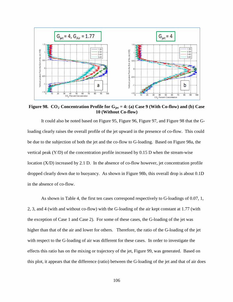
106

Figure 98. CO2 Concentration Profile for Gjet

It could also be noted based on

= 4: (a) Case 9 (With Co-flow) and (b) Case 10 (Without Co-flow)

Figure 95, Figure 96, Figure 97, and Figure 98 that the G-

loading clearly raises the overall profile of the jet upward in the presence of co-flow. This could

be due to the subjection of both the jet and the co-flow to G-loading. Based on Figure 98a, the

vertical peak (Y/D) of the concentration profile increased by 0.15 D when the stream-wise

location (X/D) increased by 2.1 D. In the absence of co-flow however, jet concentration profile

dropped clearly down due to buoyancy. As shown in Figure 98b, this overall drop is about 0.1D

in the absence of co-flow.

As shown in Table 4, the first ten cases correspond respectively to G-loadings of 0.07, 1,

2, 3, and 4 (with and without co-flow) with the G-loading of the air kept constant at 1.77 (with

the exception of Case 1 and Case 2). For some of these cases, the G-loading of the jet was

higher than that of the air and lower for others. Therefore, the ratio of the G-loading of the jet

with respect to the G-loading of air was different for these cases. In order to investigate the

effects this ratio has on the mixing or trajectory of the jet, Figure 99, was generated. Based on

this plot, it appears that the difference (ratio) between the G-loading of the jet and that of air does

107

not seem to strongly affect the mixing of the jet nor its trajectory at least at low G-loading

values.

Figure 99. Comparing Concentration Profiles at X/D = 3.4

Figure 100. CO2 Concentration Profile for: (a) Case 11 (With Co-flow),(b) Case 12 (Without Co-flow), (c) Case 13 (With Co-flow), and (d) Case 14 (Without Co-flow)

108

Figure 101. CO2

Concentration profiles at higher G-loading ranging from 100 to 1500 were illustrated in

Concentration Profile for: (a) Case 15 (With Co-flow), (b) Case 16 (Without Co-flow), (c) Case 17 (With Co-flow), and (d) Case 18 (Without Co-flow)

Figure 100 and Figure 101. Based on these plots, the jet maintained an almost straight trajectory

in the absence of the co-flow. This was expected since the jet had large momentum (large

velocity and Fr as well) at these high G-loading values. The jet maintained, in the absence of the

co-flow, relatively similar and narrow concentration profiles that decreased in the overall peak as

the stream-wise location increased due to mixing. On the other hand drastic changes occurred to

the shapes of the profiles in the presence of co-flow. In addition, at these values of G-loading,

the concentration profiles exhibited the development of two peaks. At relatively low G-loading

(GJet = 100), these peaks appeared to initially develop evenly about the center of the jet (Y/D=0).

Then, as the G-loads increased, the two peaks became more and more distinct leading to the

109

development of a double-headed profile with a larger top peak. Overall, the two peaks were

much more apparent as the G-loading increases. The development of the two peaks was only

noted, however, in the presence of co-flow. This indicates that this change in the jet’s core

structure is due to the interaction between the jet and the co-flowing air subject to G-loading. A

possible explanation of this change in the structure of the jet could be based on Schlichting and

Gersten’s observations on the flow with a curved pipe [28]. The authors noted that due to the

presence of a large centrifugal force, a secondary flow (in the pipe) emerges “outwards in the

center and inwards (towards the center of curvature) near the wall” as shown in Figure 102.

Figure 102. Flow in a Curved Pipe, after Prandtl (as inspired by Schlichting et al.’s figure)

The effects of the large centrifugal force are not only associated with the jet in the tube but

also with the air which flows in a curved cavity section. The observations noted in Figure 100

and Figure 101 could be the combination of the change in the flow structure undergone by both

the jet and the co-flow. With the formation of a large upper peak and small bottom peak within

the core of the jet, the jet mixes more with air in the bottom part of the jet and the overall

trajectory appears to be slightly moving outwards (away from the center of the curvature). In

addition, based on the overall trajectory of the jet for cases with and without co-flow, it appears

110

that, at high G-loading, the effects of buoyancy (bringing the jet down), are overcome by the

high momentum of the jet and G-loading effects.

111

V. Conclusions

V.1. Findings

The goal of this work was to understand the impact of buoyancy and G-loading on a jet in

the presence of a co-flow. Filtered Rayleigh Scattering (FRS) was used to illustrate the jet

trajectory and mixing properties of a buoyant jet using both helium and CO2

The first experiment was the Iodine filter characterization which led to the identification of

the transmission well associated with the molecular filter used in the second and third

experiments. The transmission well (or alternatively called the absorption well) defined the

range of operation of wavelength for which there was maximum blocking of background noise

and hence allowed for the collections of relevant Rayleigh scattering signal.

gases. Three

different experiments were set up, and run for that purpose. The concentration data acquired

with FRS was unique in that a continuous wave laser was used in combination with a high speed

camera to produce data at 400 Hz (80 Hz when helium was used). This enabled spatio-temporal

data collection along a linear expanse at a single stream-wise position. By passing the laser beam

through the jet twice, spatio-temporal plots at two different stream-wise positions were also

enabled. These time-resolved measurements of concentration along a line were used to

investigate the interactions of the jet with a co-flow of air for both the horizontal and G-loaded

jet configurations. The concentration of the jet was measured at several locations up to 4.4 D

away from the exit of the jet.

The second experiment involved the acquisition of concentration data of a horizontal jet in

a co-flow of air using both helium and CO2 gases. Cases with a co-flow of air and without the

co-flow were run to examine the effects on the trajectory curve and the mixing of the jet.

Processed data of Rayleigh scattering signal for cases with or without co-flow indicated that the

112

jet in general curved downwards as it traveled downstream of the jet for the case of the CO2

In addition, the shape of the trajectory was investigated through the variation of the jet

velocity, the jet to co-flow velocity ratio, the relative velocity, the Froude number, and the

Reynolds number. The Froude number definition used for comparison was based on the jet

velocity only and did not take into account the co-flow velocity. The trajectory plots were

generated by tracking the maximum value of CO

jet

due to negative buoyancy and upwards for the case of the helium jet due to positive buoyancy.

The generation of standard deviation plots of the Rayleigh scattering signal and the time histories

of the signal’s intensity at different locations along the imaging lines highlighted the time

resolved aspect of this analysis. These clues were incorporated to identify areas of significant

mixing between the jet and the co-flowing air. In general, it was deduced from the horizontal jet

experiment that the addition of the co-flow to the flow field contributed to both the straightening

of the jet trajectory and the increase of its mixing with air.

2 concentration along a strip of the Rayleigh

scattering line at multiple stream-wise locations. The trajectory analysis demonstrated that in the

presence of the co-flow, the jet velocity had an initial impact on the resultant jet location and

spread causing a more horizontal jet to convect downstream. The velocity of the jet then had the

strongest effect of all other considered parameters in shaping the trajectory of the jet. Cases with

co-flow where the Froude number was kept constant resulted in consistent trajectories and thus

impacts of buoyancy. However, at that same Froude number, the trajectory was noticeably

different when there was no co-flow. This confirmed that the traditional definition of Froude

number based on the jet velocity was the correct parameter to normalize the data; however a

correction is needed to account for the presence of a co-flow for future analysis and studies.

113

The third experiment was set up to investigate the effects of G-loading (centrifugal force)

on the jet trajectory and mixing of the jet with air. It turned out that the centrifugal force due to

the flow of the jet in a curvature changed drastically the structure of the core of the jet in the

presence of co-flow. The classical bell shaped concentration profile turned to a double headed

profile in the presence of high G-loading causing the jet to slightly move outwards (away from

the center of the curvature) on one hand and an increase in the mixing with air on the other hand.

At high G-loading where the velocity of the jet was significantly high, the effects of buoyancy

which pulled the jet down were overcome by the effects of G-loading which pushed it outwards.

V.2. Recommendations & Future Work

The idea behind imaging along two laser lines as opposed to using a sheet of laser stems

from the need to get the most out of the 12 W laser systems available in the COAL lab. Using a

sheet of laser would result in the decrease of the incident laser power and hence a lower signal to

noise ratio. However, a disadvantage of this method is that concentration data is only obtained

along the laser line which has a relatively small width. Essentially data, between the lines is

unknown. In order to bypass this problem, it is recommended for future studies to perform

multi-passes of the laser using top and bottom sets of mirrors or prisms. The idea is to collect the

Rayleigh scattering signal along multiple lines with relatively small spacing between them. That

way, data can be collected simultaneously at different stream-wise locations without the need for

a traverse unit or similar systems.

In addition, when processing data for this study, the signal to noise ratio was in some cases

low to the point that it was hard sometimes to distinguish between the Rayleigh scattering signal

associated with air and that due to CO2. Although this was not a major issue, it is recommended

for future buoyant jet in co-flow studies to use CO2 as a jet and helium as a co-flow instead of

114

air. From a fundamental stand point this would be very advantageous due to the presence of a

significantly large density gradient between CO2 and helium. Furthermore, the distinction

between the Rayleigh scattering signals associated with both gases would be relatively easy since

the Rayleigh scattering cross section of the helium is approximately about 0.6 % of that of CO2

As far as developing an equation for the Froude number that would take into account the

addition of the co-flow into the flow field, it is recommended to start with the classical definition

of the Froude number and modify it. The velocity of the co-flow has to be included in the new

formula which could have the velocity of the jet as an exponent to a factor to be determined

empirically via the analysis of multiple cases. The reason for this choice is that, in the case when

the velocity of the co-flow is zero (no co-flow), the new model collapses back to the classical

definition of the Froude number since any factor raised to zero would be one. This model could

serve as an initial guess for the development of the new formula but is not necessarily the only

one.

.

115

Bibliography

1. Subbarao, E., “The Effects of Reynolds Number and Richardson Number on the Structure of a Vertical Co-flowing Buoyant jet,” AIAA Paper 89-1800, AIAA 20th

Fluid Dynamics, Plasma Dynamics and Lasers Conference, Buffalo, New York June 12-14, 1989.

2. Xiao, J., Travis, J.R., and Breitung, W., “Boussinesq Integral Model for Horizontal Turbulent Buoyant Round Jets,” Since and Technology of Nuclear Installations, Vol. 2009, Article ID 862934.

3. Rausch, A., Fischer, A., Holger, K., Gaertlein, A., Nirsch, S., Knobloch, K., Bake, and F.,

Rohle, I., “Measurements of Density in the Outlet Nozzle of a Combustion Chamber by Rayleigh-Scattering Searching Entropy Waves, ” Proceedings of ASME Turbo Expo 2010: Power for Land, Sea, and Air, GT2010-22492, Glasgow, UK, June 14-18, 2010.

4. Eckbreth, A.C, “Laser Diagnostics for Combustion Temperature and Species”, Second

Edition, pp 3, United Technologies Research Center, Connecticut, 1996. 5. Adrian, R.J, “Twenty Years of Particle Image Velocimetry”, Experiments in Fluids, Vol. 32,

Number 2, pp 159-169, 2005. 6. Miles, R.B., Lempert, W.R., and Forkey, J.N., “Laser Rayleigh Scattering,” Meas. Sci. Tech.,

Vol. 12, pp. 33-51, 2001. 7. Miles, R.B., Lempert, W.R., and Forkey, J.N., “Accuracy Limits for Planar Measurements of

Flow Filed Velocity, Temperature and Pressure using Filtered Rayleigh Scattering”, Experiments in Fluids, Vol. 24, pp 151-162, 1998.

8. Miles, R.B, Yalin, A.P, Tang, Z, Zaidi, S. H, and Forkey, J.N., “Flow Field Imaging through

Sharp-edged Atomic and Molecular ‘Notch’ Filters ”, Measurement Science and Technology, Vol. 12, pp 442-451, 2001.

9. Polanka, M.D, Reeder, M.F, and Hartsfield, K.C, “Fundamental Issues in Integrating of UCC

Combustor with a Turbine Vane” AFIT Research Proposal to AFRL/AFIT MOA Small Grant Program, March 2010.

10. Anderson, W.S, Radtke, J.T, King, P.I, Thornburg, H, Zelina, Z., and Sekar, B., “Effects of

Main Swirl Direction on High-g Combustion”, AIAA Paper 2008-4954, 44th

AIAA/ASME/SAE/ASEE Joint Propulsion Conference & Exhibit, Hartford, Connecticut, 21-23 July 2008.

11. Mielke, A., Seasholtz, R., Elam, K., and Panda, J., “Time-average measurement of velocity, density, temperature, and turbulence velocity fluctuations using Rayleigh and Mie scattering” 2005.

116

12. Miles, R.B., and Lempert, W.R., “Flow Diagnostics in Unseeded Air”, AIAA Paper 90-0624, 28th

Aerospace Sciences Meeting, Nevada, 8-11 January 1990.

13. Sneep,M., and Ubachs, W., “Direct Measurement of the Rayleigh-Scattering Cross Section in Various Gases”, Journal of Quantitative Spectroscopy & Relative Transfer, Vol. 92, pp 293-310, 2005.

14. Meents, S., “Filtered Rayleigh Scattering Measurement in a Buoyant Flow Field,” March

2008.

15. Jenkins,T.P., and Desabrais, K.J., “Three Components Velocity Field Measurements Near a Parachute During a Drop Test,” AIAA Paper 2010-1030, 48th

AIAA Aerospace Sciences Meeting, Orlando, Florida, January 2010.

16. Cheung, B.H., and Hanson, R.K., “CW laser-induced fluorescence of toluene for time resolved imaging of gaseous flows,” Applied Physics B Lasers and Optics, Vol. 98, pp. 581-591.

17. Gebhart, B., Jaluria, Y., Mahajan, R.L, and Sammakia, B., “Buoyancy–Induced Flows and Transport”, pp 670, 1988.

18. Reeder,M.F., Huffman, R.E., Branam, R.D., Lebay, K.D., and Meents, S.M., “Mixing of Gas

phase Horizontal Laminar Jets with positive and negative buoyancy measured with Filtered Raleigh Scattering,” To appear in EXP.Fluids, published online , 19 November 2010.

19. Arakeri, J.H, Das, D., and Srinivasan, J., “Bifurcation in a Buoyant Horizontal Laminar Jet”,

Journal of Fluid Mechanics, Vol. 412, pp 61-73, United Kingdom, 2000. 20. Kumar, R., and Yuan, T.D, “Recirculating Mixed Convection Flows in Rectangular

Cavities”, AIAA Paper 88-0662, AIAA 26th

Aerospace Sciences Meeting, Nevada, 11-14 January 1988.

21. Sherif, S.A, Pletcher, R.H, “Jet Wake Thermal Characteristics of Heated Turbulent Jets in Cross Flow”, AIAA Paper A88-48776 20-34, 1988.

22. Armstrong, J., “Effect of Equivalence Ratio and G-loading on in SITU Measurement of Chemiluminescence in an Ultra Compact Combustor,” March 2004.

23. Lebay, K.D, Drenth, A.C, Thomas, L.M, Polanka, M.D, Branam, R.D, and Schmidt, J.B,

“Characterizing The Effects of G-loading in an Ultra Compact Combustor via Sectional Models”, GT2010-22723, Proceeding of the Turbo Expo 2010, 14-18 June 2010.

24. Dahm, W.J.A, Lapsa, A.P, “Hypeacceleration Effects on Turbulent Combustion in Premixed

Step-Stabilized Flames”, Proceedings of the Combustion Institute, Vol. 32, pp 1731-1738, 2009.

117

25. Seasholtz ,R.G., Buggele, A.E., and Reeder , M.F., “Flow measurements based on Rayleigh scattering and Fabry-Perot Interferometer,” Optics and Lasers in Engineering, Vol. 27, pp. 543-570, 1997.

26. Su,L.K, Helmer, D.B, and Brownell, C.J., “Quantitative Planar Imaging of Turbulent Buoyant Jet Mixing ”, Journal of Fluid Mechanics, Vol. 643, pp 59-95, 2010.

27.

28. Schlichting, H., Gersten, K., “Boundary Layer Theory”, New York, McGraw-Hill, pp 588, 1955.

Baranyi ,L., Szabó, S., Bolló ,B., and Bordás, R., “Analysis of low Reynolds number flow around a heated circular cylinder,” Journal of Mechanical Science and Technology, April 2009.

118

Vita

First Lieutenant Firas Benhassen joined the ranks of the armed forces at the age of 19. He

graduated from the Tunisian preparatory school for the military academies (Ecole Preparatoire

Aux Academies Militaires) in 2004. He then attended the United States Air force Academy

(USAFA) and graduated in 2008 with a Bachelor of Science degree in Aeronautical Engineering.

After graduation, he was stationed in Tunis at the Tunisian Air Force Academy where he served

as an Assistant Air Officer Commander (AAOC) for the freshman class. Lieutenant Benhassen

is the first Tunisian officer to attend the Air Force Institute of Technology for a Master’s in

Aeronautical Engineering. Upon completion of his assignment at AFIT, Lt Benhassen will go

back to Tunisia where he will continue to serve his country as an aircraft maintenance officer.

119

REPORT DOCUMENTATION PAGE Form Approved OMB No. 0704–0188

The public reporting burden for this collection of information is estimated to average 1 hour per response, including the time for reviewing instructions, searching existing data sources, gathering and maintaining the data needed, and completing and reviewing the collection of information. Send comments regarding this burden estimate or any other aspect of this collection of information, including suggestions for reducing this burden to Department of Defense, Washington Headquarters Services, Directorate for Information Operations and Reports (0704–0188), 1215 Jefferson Davis Highway, Suite 1204, Arlington, VA 22202–4302. Respondents should be aware that notwithstanding any other provision of law, no person shall be subject to any penalty for failing to comply with a collection of information if it does not display a currently valid OMB control number. PLEASE DO NOT RETURN YOUR FORM TO THE ABOVE ADDRESS. 1. REPORT DATE (DD–MM–YYYY)

24 03 2011 2. REPORT TYPE Master’s Thesis

3. DATES COVERED (From — To) February 2010 — March 2011

4. TITLE AND SUBTITLE Time Resolved Filtered Rayleigh Scattering Measurement of a Centrifugally Loaded Buoyant Jet

5a. CONTRACT NUMBER

5b. GRANT NUMBER

5c. PROGRAM ELEMENT NUMBER

6. AUTHOR(S) Firas Benhassen, 1st

5d. PROJECT NUMBER

Lt, TUNAF 5e. TASK NUMBER

5f. WORK UNIT NUMBER

7. PERFORMING ORGANIZATION NAME(S) AND ADDRESS(ES) Air Force Institute of Technology Graduate School of Engineering and Management (AFIT/ENY) 2950 Hobson Way WPAFB OH 45433-7765

8. PERFORMING ORGANIZATION REPORT NUMBER AFIT/GAE/ENY/11-M01

9. SPONSORING / MONITORING AGENCY NAME(S) AND ADDRESS(ES) Directorate Aerospace, Chemical, and Material Sciences Air Force Office of Scientific Research Tele: (703) 696-8478 DSN: 426-8478 Fax: (703) 696-8451 Dr. Julian Tishkoff 4015 Wilson Boulevard, Room 713 Arlington, VA 22203-1954 E-mail: julian.tishkoff@afosr.af.mil

10. SPONSOR/MONITOR’S ACRONYM(S) AFOSR 11. SPONSOR/MONITOR’S REPORT NUMBER(S)

12. DISTRIBUTION / AVAILABILITY STATEMENT APPROVED FOR PUBLIC RELEASE; DISTRIBUTION UNLIMITED

13. SUPPLEMENTARY NOTES This material is declared a work of the U.S. Government and is not subject to copyright protection in the United States.

14. ABSTRACT

The combustion process within the Ultra-Compact Combustor (UCC) occurs in the circumferential direction. The presence of variable flow density within the circumferential cavity introduces significant buoyancy issues. On the other hand, G-loading caused by the presence of centrifugal forces, ensures the circulation of the flow in the circumferential cavity and enhances the completion of the combustion process before allowing the exit of the hot gases to the main flow. The coupling between buoyancy and high G-loading is what predominately influences the behavior of the flow within the UCC. In order to better understand the combustion process within the UCC, three different experiments were run. The overall objective of these experiments is to investigate the effects of both buoyancy and G-loading on the trajectory and the mixing of a jet in a co-flow. The first experiment involved setting up the Filtered Rayleigh scattering (FRS) technique to be used in this research. Then, using horizontal and curved sections, two types of experiments were run to characterize and measure both G-loading and buoyancy effects on the overall behavior of a jet in a co-flow of air. Measurements were made using an FRS set up which involved a continuous wave laser and a high speed camera showing adequate signal to noise ratio at 400 Hz. Collected time resolved images allowed for the investigation of the effects of G-loading and buoyancy on the mixing properties and trajectory of the jet.

15. SUBJECT TERMS Filtered Rayleigh scattering, Continuous Wave Laser, Horizontal Buoyant Jet, G-loaded Buoyant Jet 16. SECURITY CLASSIFICATION OF: 17. LIMITATION

OF ABSTRACT UU

18. NUMBER OF PAGES 133

19a. NAME OF RESPONSIBLE PERSON Dr. Marc Polanka

a. REPORT U

b. ABSTRACT U

c. THIS PAGE U

19b. TELEPHONE NUMBER (Include Area Code) Tele: (937)255-3636, ext 4714 Email: marc.polanka@afit.edu

Standard Form 298 (Rev. 8–98) Prescribed by ANSI Std. Z39.18