i

UNIVERSIDAD POLITÉCNICA DE MADRID

ETSIT DE TELECOMUNICACIONES

TOT & TOK PROJECT

CORPORACIÓN DE ALTA

TECNOLOGÍA PARA LA DEFENSA

REAL TIME SCAN CONVERSION

IMPLEMENTATION

Master degree final work.

Author:

Darwin Leonardo Gómez Pinzón

2015

TUTOR: Jose Maria Peña Espartero, ART Research & Development

Máster en radar, tecnologías, equipos y diseño de sistemas

ii

ACKNOWLEDGEMENTS

I would like to express my sincere gratitude to my family for their unconditional support. To my parents Blanca y Guillermo, their guidance helped me to research my dreams and professional ambitions.

To UPM university and their teachers for an excellent job, a wise vision and hard work has exceeded our expectations.

My sincere thanks to ART team especially my tutor. I could not have imagined having a better advisor.

I thanks CODALTEC to believe in the technological development of Colombia and built a better future to Colombian people.

iii

INDEX

ACKNOWLEDGEMENTS .............................................................................. ii

INDEX ............................................................................................................ iii

SUMMARY ..................................................................................................... v

KEY WORDS ................................................................................................ vi

FIGURE LIST ................................................................................................ vii

TABLE LIST .................................................................................................. ix

OBJECTIVES ................................................................................................. x

INTRODUCTION .......................................................................................... xi

1. CHAPTER 1- THEORETICAL BACKGROUND ........................... 1

1.1 Radar Definitions ..................................................................... 1

1.2 High Resolution Radars ................................................................ 1

1.3 Radar Matrix.................................................................................. 2

1.4 Raw Video ..................................................................................... 3

1.5 Clutter Map .................................................................................... 3

1.6 GPU .............................................................................................. 5

1.7 Primitive Definition ........................................................................ 5

1.8 Rendering ...................................................................................... 5

1.9 Texturing Objects .......................................................................... 6

1.10 Parallel Processing ..................................................................... 6

1.11 Real Time System ....................................................................... 7

2. CHAPTER 2- SCAN CONVERSION DEFINITIONS .................. 10

2.1 Direct Coordinate Transform Problem ........................................ 12

2.2 High Data Process ...................................................................... 13

2.3 Interpolation Algorithms .............................................................. 14

2.4 Texture Algorithm ........................................................................ 15

3. CHAPTER 3- SCAN CONVERSION IMPLEMENTATION ......... 17

3.1 Textured Scan Conversion Implementation ............................... 18

3.2 Parallel Implementation .............................................................. 22

iv

3.3 Results ........................................................................................ 24

3.4 Real-Time Capability ................................................................... 30

3.5 Scan Conversion as part of a Command and Control Software 34

4. CHAPTER 4- OPTIMIZATION PROCESS ................................. 40

4.1 Re – Define Cell Power Level Resolution ................................... 40

5. CHAPTER 5- CONCLUSIONS ................................................... 43

BIBLIOGRAPHY .......................................................................................... 44

v

SUMMARY

The Cartesian representation is the most intuitive and easy way to display the detections provided by the radar. In high-resolution radar systems there is a bottleneck when raw video or clutter map is processed due to the high density of data. To graph this information in real time, by a conventional PC, is necessary using the resources of the PC graphics card (GPU), through specialized APIs.

To achieve the requirement of real time and avoid graphics defects, from a direct coordinate transformation (Moiré patterns), an algorithm based on textures is used, reaching excellent performance as a graphic interpolator and because it is much faster than traditional algorithms [1]. The use of parallelization is evaluated to further improve runtimes and the consequences of truncated resolution in the received power magnitude was also evaluated.

This work is part of command and control console that is being implemented in ART (Advance Radar Technologies) radars, but it could be use as well to upgrade consoles in old radars systems that use graphic hardware with low performance.

La representación cartesiana es la forma más intuitiva y sencilla de mostrar al operador las detecciones y blancos proporcionados por el radar. En sistemas radar de alta resolución, existe un cuello de botella asociado al procesamiento de video crudo o mapa de clutter debido a la gran densidad de datos involucrados. Por lo que para procesar dicha información en tiempo real, por medio de un PC convencional, se hace necesario utilizar los recursos de la tarjeta gráfica del PC (GPU) a través de API´s especializadas.

Para alcanzar el requisito de tiempo real y eliminar los defectos gráficos, propios del cambio de coordenadas directo (Patrones de Moiré), se utiliza un algoritmo basado en texturas que alcanza un excelente rendimiento como interpolador gráfico y porque es un algoritmo mucho más rápido que los algoritmos tradicionales [1]. Así mismo se evalúa la utilización de paralelización para mejorar los tiempos de ejecución y las consecuencias derivadas de la disminución de la resolución en la magnitud de potencia recibida.

Este trabajo hace parte de la consola de explotación y control que será implementada en los radares de ART (Advance Radar Technologies), pero puede ser utilizada también en la actualización de consolas de sistemas radar antiguos que utilicen hardware gráfico de bajas prestaciones.

vi

KEY WORDS

High resolution radar (HRR), Scan conversion, Graphic texture, Real-time, Graphic processor unit (GPU), Clutter map, Radar matrix, Interpolation, Texture algorithm, Task parallel library (TPL), Blob, Plot, Track, Colorbar.

Radar de alta resolución (HRR), Scan Conversion, Textura gráfica, Tiempo real, Unidad grafica de procesamiento (GPU), Mapa de clutter, Matriz radar, Interpolación, Algoritmo de texturizado, Librería de tareas en paralelo (TPL), Blob, Plot, Track, Paleta de colores.

vii

FIGURE LIST

Page

Figure 1 Radar Matrix (Polar Coordinate). ..................................................... 2

Figure 2 Radar Receptor architecture ........................................................... 3

Figure 3 IIR filter architecture used to calculate clutter map.......................... 4

Figure 4 Texture Coordinates. ....................................................................... 6

Figure 5 Real - Time modelling. [11] ............................................................. 7

Figure 6 (Above) Radar Data Matrix representation (range vs. azimuth) versus (Below) Cartesian Coordinates Representation after scan conversion ......................................................................................... 11

Figure 7 Undesirable Scan Conversion graphics artefact (Moiré Patterns).13

Figure 8 Linear Interpolation Algorithm [12] ................................................. 14

Figure 9 Bilinear Interpolation Algorithm [12] ............................................... 15

Figure 10 Graphic representation of radar data matrix without Scan Conversion. ....................................................................................... 15

Figure 11 Textured Algorithm Process. ....................................................... 16

Figure 12 Textured Algorithm Process Result. ............................................ 16

Figure 13 Scan Conversion Software hierarchy .......................................... 17

Figure 14 Texture and pixel screen coordinate relationship. ....................... 19

Figure 15 Example how use CustomVertex structure. ................................ 20

Figure 16 Combining Vertex ........................................................................ 21

Figure 17 Textured scan conversion test. .................................................... 22

Figure 18 Textured Scan Conversion to azimuth Sectors (10° and 45°). ... 25

Figure 19 Textured Scan Conversion to azimuth Sectors (270° and 360°). 26

Figure 20 Final textured scan conversion result without Moiré pattern. ..... 27

Figure 21 Real-Time model, Core 1. .......................................................... 30

Figure 22 Real - Time model, Core 2. ......................................................... 31

Figure 23 Real-Time model both cores. ...................................................... 32

Figure 24 Render of plots and tracks using DirectX. .................................. 35

Figure 25 Plots and tracks along with background map. ............................ 36

viii

Figure 26 Scan conversion implemented in command a control software. 37

Figure 27 Zoom implementation to textured scan conversion. ................... 38

Figure 28 Different colour palettes implementation. ................................... 39

Figure 29 Textured scan conversion with 16 bits (Above) and 32 bits (Below) .......................................................................................................... 41

ix

TABLE LIST

Table 1 Time-loading factor interpretation ..................................................... 9

Table 2 Result Time Table GPU Implementation ........................................ 28

Table 3 Result Time Table Parallel implementation. ................................... 29

Table 4 Result Time Table GPU Implementation ........................................ 29

Table 5 Time loading factor of real time process ......................................... 33

Table 6 Time loading factor to Core 1.......................................................... 33

Table7 Time loading factor to Core 2, using parallel and non-parallel process. .......................................................................................................... 34

Table 8 C # Type Number description. [15] ................................................ 40

Table 9 Result time table with less value resolution. ................................... 42

x

OBJECTIVES

Global Objective:

∼ Develop a real time raw video scan conversion for high resolution radars.

Specific Objectives:

∼ Truncate power level resolution to reduce the size of data to process.

∼ Use interpolation algorithm to fulfil empty pixels as result of a direct scan conversion process. (Moiré Pattern).

∼ Analyse and compare two different implementation methods whit GPU and parallel algorithms.

∼ Scan Conversion implementation in conventional PC´s.

xi

INTRODUCTION

Scan conversion is a bottleneck in the display of high resolution radar data. New ways to afford this process are necessary to meet real time visualization requirement, necessary in critical applications like raw video or clutter map visualization.

High data density is the main problem to develop scan conversion in high resolution radar where there are more radar cells resolutions than pixels in a screen, and especially when it is also necessary to avoid a graphic artefact known like Moiré pattern.

Recently, power graphic API`s has been great advances in the performance of graphics processing through PC`s graphics cards (GPU). The aim of this work is to use this potential and advantages in order to develop scan conversion process in real time. Nowadays images textured, using API´s, is being used like assisted interpolation algorithm in order to make faster scan conversion process, like it has been demonstrated in previous studies [1].

Two different implementations are analyzed to compare their runtime performance to real-time Clutter Map visualization, using specific graphic hardware (GPU) and with parallel process. Consequences of reduce resolution in the received power magnitude was also evaluated, like a possible way to reduce computational load. Results are shown, compared and discussed.

This work is part of a command and control software, it shows user blobs, plots and tracks as well. Show map clutter along with the rest of data levels is an important analysis capability to training user. Overall this command a control software is useful in old radar system upgrade, where low performance graphics consoles could be replaced for an inexpensive and more powerful conventional PC.

1

1 . C H A P T E R 1 - T H E O R E T I C A L B A C K G R O U N D

This chapter describes basics concepts that are using to develop scan conversion. As well the specific tools to analyze real time graphic development.

1.1 Radar Definitions

Radar is a detection system that uses radio radio waves to determine the range, direction, or speed of objects. In high resolution radars a wide band signal is sent by an antenna. Returns or echoes, from this signal, are processed in a functional block, usually called Signal Processor, to determine targets position and speed in the radar exploration area.

When echoes exceed a threshold in one resolution cell, it is defined like DETECTIONS.

In high resolution radars, wide targets could generates several DETECTIONS, this collections of DETECTIONS is called BLOBS. After an association detection process, BLOBS are associated to a single targets called PLOTS, through extractor Data block.

Using a spatial correlation from every PLOT, in order to avoid false alarms, Data Processor functional block, define TRACKS.

1.2 High Resolution Radars

These kinds of radars are characterized because the size of the resolution cell could be much lower than the size target that is trying to be detected. It means that one targets could be detected in more than one resolution cell.

In general the size of a resolution cell depends inversely of bandwidth signal that why high resolution radars (HRR) works whit large bandwidth

2

signals than made very small cell resolutions. On the other hand large bandwidth signal makes radar to have low probability of interception because the signal power is distributed in all the bandwidth.

1.3 Radar Matrix

Signal echoes information are collected in a data matrix, where columns represent angles and rows represent range. This is how the targets DETECTIONS are stored in memory and is the way how radar gives targets information to graphical representation radar system.

Figure 1 Radar Matrix (Polar Coordinate).

The total number of resolution cells is the multiplication between the number of azimuth cells (Na) and the number or range cells (Nr).

����� �������� ��� = �� ∗ ��

3

1.4 Raw Video

Raw video is the information contained in the radar echo signal when it is connected directly to the video output without any signal process over this signal. It is the “traditional” type of radar presentation [2] . Next Image shows a basic radar receptor architecture. Power echo of the n cell resolution, P(n), is an analog signal that is digitalized by ADC (Analog Digital Converter).

Figure 2 Radar Receptor architecture

Raw video displays require a human interpretation. It means that only a trained user is able to distinguish between targets and clutter or noise.

Process and display Raw video using scan conversion is a complex task to high resolution radar, due to the large amount of data involved.

1.5 Clutter Map

Clutter is the term used to describe any object that may generate unwanted radar returns that may interfere whit normal radar operations [3]. Clutter has an adverse effect in radar´s ability to detect targets.

Clutter Map is the power clutter distribution that radar system receives from the scan area. Clutter Map is very useful to fight against adverse Clutter

4

effect, because establish a power threshold that targets must overcome in order to declare it like a real target.

Clutter value is the averaging power level in each cell resolution. Clutter map is calculated by IIR filter (low pass band filter) whit next expression:

�(�) = �� ∗ �(�) + �1 ∗ �(� − 1)

Where,

�(�): � ���� ������� ���� �� �ℎ� ��� ��������� �

�(�): � �ℎ� ����� ���� �� �ℎ� (�) ��� ��������

�(� − 1): � �ℎ� ����� ���� �� �ℎ� ( � − 1 ) ��� ��������

�� , �1: �������

Figure 3 IIR filter architecture used to calculate clutter map.

Scan conversion process of Clutter map as complex as raw video. In fact in the specific case of radar on which this study is based, process clutter map is more complicated because it has a 32 bit word size while raw video is 16 bit size.

5

1.6 GPU

GOU is defined as a hardware graphical processing unit. It is a sophisticated processor offering multiple cores and pipelines. This unit has its own graphics memory (video ram or VRAM) and support simple control flow structures and several mathematical operations, many of which are devoted to graphic specific functions. [4]

1.7 Primitive Definition

A 3D primitive is a collection of vertices that form a single 3D entity. The simplest primitive is a collection of points in a 3D coordinate system, which is called a point list.

Habitually, 3D primitives are polygons. A polygon is a closed 3D figure defined by at least three vertices (usually called Vertex). The simplest polygon is a triangle. Triangles are using to compose most of its polygons because all three vertices in a triangle are guaranteed to be coplanar. Rendering nonplanar vertices is inefficient but triangles can be combined to form large, complex polygons and meshes. [5]

1.8 Rendering

Rendering is the process to create an image on the display screen. Rendering has 4 stages:

1. Transform and process individual vertices.

2. Convert each connected primitive vertices into fragments. Fragment is

a Pixel with attributes (colour, position, texture).

3. Process individual fragments.

4. Fragments are combined into 2d colour pixel for the output display. [6]

6

1.9 Texturing Objects

Using an informal language “texture” term usually refer to the roughness of an object. In a 3D graphic language “texture” are 2D bitmaps that cover a primitive in order to simulate a real life texture. [7]

Four normalized vertices must be defined to place the texture on the primitive (See next Figure). This coordinates are used to map each pixel on the screen with its corresponding texture element (Texel). This Texel contains the colour information that create a texture effect.

Figure 4 Texture Coordinates.

1.10 Parallel Processing

Many computers have more than one cores (CPU) that enables multiple threads that could be executed simultaneously. Computers in the near future are expected to have significantly more cores. To take advantage of present and future hardware, the code can be parallelized to distribute the data processing into multiple processors. [8]

7

1.11 Real Time System

A real-time system is a system that must satisfy explicit (bounded) response-time constrains or risk severe consequences, including failure. Failed system is a system that can not satisfy one or more of the requirements stipulated in the formal system specification. [9]

Depending of timing requirement there are two basic real-time categories. Hard real-time system has to produce to a situation before a specified deadline. A Soft real-time system responds to a situation after the deadline. [10]

Real-time system is usually modelled by a set of concurrent task, where every task consumes a quantity of computational resources.

Figure 5 Real - Time modelling. [11]

Release time (ri): Task is ready to be executed.

Start time (Si): Time when the execution start.

Computation time (Ci): Task execution time.

Finishing time (fi): Task finishes its execution.

Response time (Ri): Task´s time spends since release time. [Ri= fi-ri]

Absolute deadline (di): Task must be complete by this time.

8

Relative deadline (Di): Relative to the release time, task must be complete by this time. [Di = di-ri]

Laxity (slacki): Maximum time task can be delay to still finish within its dead line. [slacki= di-fi]

Lateness (Li): Task´s delay before its deadline.[Li= fi-di]

The CPU utilization (time-loading factor), U, is the way to measure real time system performance. System time-loading factor (U) is calculated using the contribution of individual time-loading factor (Ui) of each task in the system.

Ui = ei /pi

Where,

ei: Maximum task runtime

pi: Task Period

Then,

U= ∑ &� = ∑ ei /pi

9

Next table describe the time-loading factor interpretation.

Time-loading factor (U) Interpretation

>100% Highly used system. It is undesirable because system could be unstable.

80% Acceptable to system that do not expect to grow.

70% It is a desirable and powerful result. [9]

68% - 26% Safe

<25% Excessive processing power

Table 1 Time-loading factor interpretation

10

2 . C H A P T E R 2 - S C A N C O N V E R S I O N D E F I N I T I O N S

Radar scan conversion is defined as a radar data coordinate transform from Polar into Cartesian. Typically, radar provides information as it was stored, azimuth-range (Polar coordinate), while the computer graphics systems use Cartesian coordinates.

Next figure shows a Polar radar information representation in a computer screen (above) versus a Cartesian representation after scan conversion transformation example (below). It is a Matlab scan conversion implementation. In this case Matlab makes interpolation automatically but runtime could spend more than 10 seconds, depends of cell resolution quantity. It shows how hard is to reach real time capability when data arrive every second.

11

Figure 6 (Above) Radar Data Matrix representation (range vs. azimuth)

versus (Below) Cartesian Coordinates Representation after scan conversion

12

Point representation in Polar coordinate (r,θ).

� = �����

' = �(�)�ℎ

Point representation in Cartesian coordinate (x,y).

* = ��)������ �� + �*�

, = ��)������ �� - �*�

Next mathematics expression define direct coordinate Polar – Cartesian transformation as:

* = � ∗ �� '

, = � ∗ .�� '

2.1 Direct Coordinate Transform Problem

Coordinate transform operation produce a serious and undesirable graphic artefact usually called Moiré Patterns. During coordinate transform screen pixels keep empty (without visual data) because there is not a 1 to 1 relation between Polar and Cartesian coordinates points. This visual defect is shown in the next Figure.

13

Figure 7 Undesirable Scan Conversion graphics artefact (Moiré

Patterns).

2.2 High Data Process

The order of the number of resolution cells for high-resolution radar are millions, it means that scan conversion algorithm should process millions of operations in less time than the antenna rotation, to be a real-time system. This is not a trivial problem to handle in a conventional computer.

Also, it is necessary to consider that the number of pixels in a typical screen size is much less than the number of resolutions cells to be represent graphically. It is clearly an important challenge. For example the high resolution radar used in this study has 888 azimuth cells and 8192 range cells. It means 7’274.496 resolution cells while a HD screen just has 1090 x 1920 pixels that would graphic only 1’393.200 resolution cells.

14

2.3 Interpolation Algorithms

Interpolation allows to represent high density of data in a less resolution screen. As well scan conversion produce pixel without information (Moiré Patterns). Interpolation techniques are commonly used to complete the information in every pixel of the final image. Next, it is described the most common interpolation algorithms:

- Nearest: The first and simple method. In this method the closest data point to the needed pixel is used. There is not interpolation. So the value (information, colour, texture, etc) of the closest sample become the value of the blank (needed) pixel. [1]

- Linear Interpolation: It implements a linear interpolation between 2 closer points of needed pixel. With the interpolation information creates the pixel needed.

Figure 8 Linear Interpolation Algorithm [12]

- Bilinear Interpolation: This methods use 4 adjacent vectors to compute the pixel value. Three linear interpolations must be performed in order to obtain pixel value.

15

Figure 9 Bilinear Interpolation Algorithm [12]

2.4 Texture Algorithm

This algorithm use texture mapping over raw video (Polar coordinates) sector to fit the dimensions of the scan converted image. This algorithm was used like assisted interpolation algorithm in order to make faster scan conversion process, like it has been demonstrated in previous studies [1].

Step 1: Capture radar matrix data from the radar system. It capture must be convert in an image file.

Next image show an example, a matrix without scan conversion process.

Figure 10 Graphic representation of radar data matrix without Scan Conversion.

16

Step 2: Divide data matrix in azimuth sectors. Every division is the polar coordinate representation of an azimuth sector from the radar matrix.

Step 3: Individual sector describes a rectangular shape that could be defined by 4 vertices. Texture is mapped in each vertex using this procedure: Tow vertices, the most remote ones, keep outside (P1 and P2), the remaining vertices (P3 and P4) are placed at the origin (reception antenna rotation point) as it see in next figure.

Figure 11 Textured Algorithm Process.

Step 4: Assemble each sector in the correct order.

Figure 12 Textured Algorithm Process Result.

17

3 . C H A P T E R 3 - S C A N C O N V E R S I O N I M P L E M E N T A T I O N

This chapter describes the textured scan conversion algorithm implementation, for a high resolution radar with more than 7 million of resolutions cells, using C# as programming tool. C# is an object - oriented programming language to quickly applications development on the Microsoft .NET Platform [13]. To access to the GPU computer resources was necessary use a Microsoft rich multimedia collection of API´s (Application Programming Interface) specifically designed to handling high performance graphics applications, called DirectX. DirectX allows developers an easy and fast way to get complex or simple graphics animation on screen using PC´S GPU resources [7]. This means that general propose PC processor and ram memory do not have to support graphics task, it avoid that PC get slow and assure that real time process have done properly.

Software consist in three main parts, layer, controller and scene that allows show multiple data levels, and then it is possible to combine different information on the same screen area and with a specific transparency in order to avoid visual interferences. Next image shows classes software hierarchy.

Figure 13 Scan Conversion Software hierarchy

18

Controller: This class is responsible to control which layer are shown to the user and control graphical aspects like Zoom, Colour Pallet, etc.

Layers: Every layer is responsible to render specific graphic information on the screen using DirectX. For example Track Layer renders each track that it being receiving by radar system, but only tracks.

Scene: The software developed has the capability to render tracks, plots, blobs, clutter map and geographic maps. Scene combines these levels of radar data.

3.1 Textured Scan Conversion Implementation

The first task is to load data from a binary file that radar system give thought a TCP/IP connexion. Clutter Map binary file contains one main header with general information about data that it is being receiving. There is a secondary header for every azimuth resolution (Na) that includes (Nrange) clutter power level cell range resolution data.

CustomVertexPositionTextured (float xValue, float yValue, float zValue, float u, float v)

Last is the C# structure that describes a custom vertex format structure that contains position and one set of texture coordinates. [14]

CustomVertexPositionTextured structure allows to rendering a texture on a primitive structure, from an image generated in task 2 (Chapter 2). xValue, yValue, zValue represent the screen pixel region where texture primitive is being render. u and v are vector that represent the image portion (percentage)that will be used as texture. Next figure shows the relationship between texture coordinate and pixel screen coordinate (For example widthSize x heightSize screen).

19

Figure 14 Texture and pixel screen coordinate relationship.

Three CustomVertexPositionTextured structure describes a triangle, Tow triangles describe a rectangle. Next it describes an example, taking a rectangle region where 50% of the image is textured and rendered on 50% of the screen.

Vertex [0] = new CustomVertex.PositionTextured( 0.0f , heightSize/2 , 1.0f, 0.0f, 0.0f);

Vertex [1] = new CustomVertex.PositionTextured( 0.0f , - heightSize/2 , 1.0f, 0.0f, 1.0f);

Vertex [2] = new CustomVertex.PositionTextured( widthSize/2 , heightSize/2 , 1.0f, 1.0f, 0.0f);

Vertex [3] = new CustomVertex.PositionTextured( 0.0f , - heightSize/2 , 1.0f, 0.0f, 1.0f);

Vertex [4] = new CustomVertex.PositionTextured( - widthSize/2 , - heightSize/2 , 1.0f, 1.0f, 1.0f);

Vertex [5] = new CustomVertex.PositionTextured( widthSize/2 , heightSize/2 , 1.0f, 1.0f, 0.0f);

Next image shows graphically the process described before.

20

Figure 15 Example how use CustomVertex structure.

21

In order to make a scan conversion using texture, it is necessary to combine vertices to create a triangle area that represent an azimuth sector. Next image shows how to combine vertex and the final effect:

Figure 16 Combining Vertex

Coordinate screen for Vertex [0], Vertex [2] and Vertex [5] must be set in x= 0 ,y=0 ) (reception antenna rotation point). Please see Chapter 2, step 3.

Finally assemble each sector in the correct order. Please see Chapter 2, step 4.

To ensure that scan conversion algorithm is doing well, it is necessary to use tests cards. Card test is a radar matrix made by software where specifics patterns are used to ensure that scan conversion algorithm works properly. In this case the result of the scan conversion is well known (reference) and it is compare with the result of textured scan conversion. Next image shows at left the card test matrix (Na azimuth cells = 888, Nr range cells = 8192) and the textured scan conversion result at right.

22

Figure 17 Textured scan conversion test.

It is possible to see that textured scan conversion does not distort the pattern. Greyscale sector are show properly and the width of each sector is larger as it moves away from the centre.

3.2 Parallel Implementation

Using multiple threads is a powerful way to improve runtime performance of applications. Task Parallel Library (TPL) is a set of public types and APIs to simplifying the process of adding parallelism to applications in .NET platforms.

Task Parallel Library (TPL) allows to describe parallel “for” loops. These kinds of loops are usefull when program goes over a radar matrix. For example next code represent a normal “for” loop where tasks must be done in each range of each azimuth (Image generation class uses a loop like that). In this case program does not use multiple threads:

23

for (int i=0; i < AzimuthLast ; i++ )

{

for (int y=0; y < RangeLast ; y++ )

{

//Tasks with RadaMatrix [i,y];

}

}

A simple change is done in order to use TPL and allows program that multiples cores develop tasks on the same radar matrix at the same time.

Parallel.For (0; AzimuthLast ; i=>

{

for (int y=0; y < RangeLast ; y++ ) // AzimuthLast = 8192

{

//Tasks with RadaMatrix [i,y];

}

});

24

3.3 Results

Next it is described general purpose PC characteristics that has been used for the scan conversion implementation.

Processor: Intel Core i5-4440. @ 3.10Ghz

Ram Memory: 8Gb

Operative System: Microsoft Windows 8.1

GPU: NVIDIA GeForce GT 625, Video Memory 4043MB

In this particular case an ART Mid–range radar has been used as main sensor platform. Next, it´s described the radar characteristics:

∼ Continuous Wave Signal.

∼ Maximum Range 5 Km.

∼ High Resolution Radar.

888 azimuth cell resolution, Then 360°/ 888 = 0.40°

8192 range cell resolution, Then 5 Km/ 8192 = 0.6 m

∼ Total cells resolution (888 x 8192) = 7´274.496

∼ Low Probability of Interception (LPI).

Textured scan conversion was applied in a real clutter map matrix. Next figures shows the result with azimuth sectors from 0° to 10°, 45°, 270° and 360°.

Individual 2° azimuth sector width is used to complete all 360° azimuth sector. Azimuth of individual sectors must be small in order to makes a circular shape when individual azimuth sectors are combined.

25

Figure 18 Textured Scan Conversion to azimuth Sectors (10° and 45°).

26

Figure 19 Textured Scan Conversion to azimuth Sectors (270° and 360°).

27

Figure 20 Final textured scan conversion result without Moiré pattern.

28

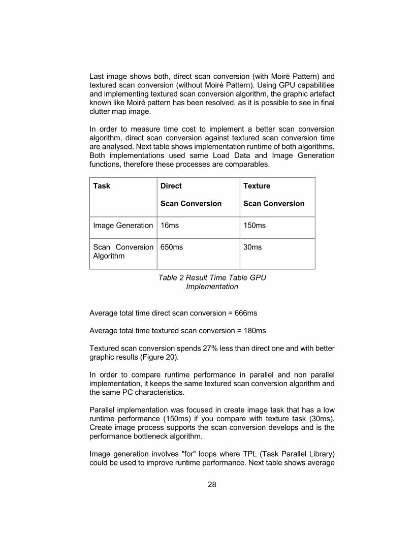
Last image shows both, direct scan conversion (with Moiré Pattern) and textured scan conversion (without Moiré Pattern). Using GPU capabilities and implementing textured scan conversion algorithm, the graphic artefact known like Moiré pattern has been resolved, as it is possible to see in final clutter map image.

In order to measure time cost to implement a better scan conversion algorithm, direct scan conversion against textured scan conversion time are analysed. Next table shows implementation runtime of both algorithms. Both implementations used same Load Data and Image Generation functions, therefore these processes are comparables.

Task Direct

Scan Conversion

Texture

Scan Conversion

Image Generation 16ms 150ms

Scan Conversion Algorithm

650ms 30ms

Table 2 Result Time Table GPU Implementation

Average total time direct scan conversion = 666ms

Average total time textured scan conversion = 180ms

Textured scan conversion spends 27% less than direct one and with better graphic results (Figure 20).

In order to compare runtime performance in parallel and non parallel implementation, it keeps the same textured scan conversion algorithm and the same PC characteristics.

Parallel implementation was focused in create image task that has a low runtime performance (150ms) if you compare with texture task (30ms). Create image process supports the scan conversion develops and is the performance bottleneck algorithm.

Image generation involves "for" loops where TPL (Task Parallel Library) could be used to improve runtime performance. Next table shows average

29

runtime results with and without TLP in “for” loops that does over matrix radar.

Result Time Table

Process Whit Parallel process.

Without Parallel process.

Image Generation 47ms 150ms

Table 3 Result Time Table Parallel implementation.

Image generation has improved from 150ms to 47ms using parallel process. It means 31% faster to parallel process.

Parallelizing image generation task improve general runtime of the textured scan conversion. Next table shows the general average runtime between textured scan conversion using TPL and without it.

Task Parallelized Non Parallelized

Image generation 47ms 150ms

Texture Scan conversion

30ms 30ms

Table 4 Result Time Table GPU Implementation

Average runtime textured scan conversion with parallel tasks = 77ms

Average runtime textured scan conversion without parallel tasks = 180ms

It means that parallelizing task improve the textured scan conversion tie performance making it 42% faster. And it is 115% faster than direct scan conversion as well.

30

3.4 Real-Time Capability

Rotation speed of the radar is 60 RPM it means that update time of raw video is 1 second. Once one rotation is complete clutter map data is send by a TCP/IP link. It download process spend in average less than 800ms and it is running in a different core.

A real-time model is developed in order to analyse the textures scan conversion real-time performance for each core.

Figure 21 Real-Time model, Core 1.

Core 1.

Task: Download data.

Release time (r1) = 1000 ms.

Start time (s1) = 1000 ms.

Computation time (C1) = 800 ms.

Finishing time (f1) = 1800 ms.

Response time (R1) = f1-r1 = 800 ms.

Absolute deadline (d1) = 2000 ms.

31

Relative deadline (D1) = d1-r1 = 1000 ms.

Laxity (slack1) = d1-f1 = 200 ms.

Lateness (L1) = f1-d1 = -200 ms.

Figure 22 Real - Time model, Core 2.

Core 2.

Tasks: Processing data, Generate image, textured scan conversion.

Release time (r2) = 1800 ms.

Start time (S2) = 1800 ms.

Computation time (C2) = 738 ms.

Finishing time (f2) = 2538 ms.

Response time (R2) = f2-r2 = 738 ms.

Absolute deadline (d2) = 2800 ms.

Relative deadline (D2) = d2-r2 = 1000 ms.

32

Laxity (slack2) = d2-f2 = 262 ms.

Lateness (L2) = f2-d2 = -262 ms.

Figure 23 Real-Time model both cores.

33

Time-loading factor provides information about real – time process stability.

Task Task runtime (ei), [ms]

Task period(pi), [ms]

Time-loading factor (Ui), [%]

Down Load data 800 1000 80% CORE

1

Load data time 624 1000 62%

CORE

2

Image generation

150 1000 15%

Image generation (Parallelized)

63,87166667 1000 6%

Textured scan conversion

50,743 1000 5%

Table 5 Time loading factor of real time process

CORE 1 Total Time-loading factor

(Ui), [%] Total Tasks Runtime

80% 800

Table 6 Time loading factor to Core 1.

34

Total Time-loading factor

(Ui), [%]

Total Tasks

Runtime

CORE 2

Non Parallelized 82% 824,743

Parallelized 74% 738,6146667

Table7 Time loading factor to Core 2, using parallel and non-parallel process.

None of the cores reaches a critical loading factor level. It could be consider like stable processes. [9]

3.5 Scan Conversion as part of a Command and Control Software

Blobs, plots and tracks have less computational load, and reach real -time capability present less complications, but steel correct representation and correct time of representation are warranty that command and control software user, has the best tool to understand the information that radar is providing. Next figure is an example of how data sent by radar (plots and tracks), are rendered by command a control software.

35

Figure 24 Render of plots and tracks using DirectX.

As the same way, geographic maps are so useful to establish visual references, distance and times between targets and radar. Next figure has a background map along with radar data, blobs and tracks.

36

Figure 25 Plots and tracks along with background map.

The capability to show the clutter map with the rest of data levels (blobs, plots and tracks) is an important analysis capability to trained user. For example a low speed target in high clutter environment could be not declared like a track, but clutter map is able to show it. Next figure shows part of command a control software that implement textured scan conversion and the graphic representation of blobs, plots and tracks at the same time.

37

Figure 26 Scan conversion implemented in command a control software.

Zoom is a practical capability in data radar representation. However, the implementation is a challenge due to the large amount of information to be reprocessed. Using GPU capabilities and a textured algorithm allows zoom in and zoom out faster enough to users could not detect any delay.

38

Figure 27 Zoom implementation to textured scan conversion.

The implementation of different colour palettes to represent plots and clutter map power value makes the software flexible to user preferences. It is possible to choose between the most popular colorbars like rainbow, perceptual or summer.

39

Figure 28 Different colour palettes implementation.

40

4 . C H A P T E R 4 - O P T I M I Z A T I O N P R O C E S S

4.1 Re – Define Cell Power Level Resolution

The clutter power level of each cell resolution is represented by a 32 Byte word. It represents a very high exactitude level. Otherwise in order to reduce computational load, it is possible to reduce the word. Next table describes possible types of data to use and their sizes.

Type Range Approximations

Size Resolution

short -32,768 to 32,767 16 3 Digits

float -3.4 × 1038to +3.4 × 1038

32 7 Digits

double ±5.0 × 10−324 to ±1.7 × 10308

64 15-16 Digits

Table 8 C # Type Number description. [15]

Human eyes could distinguish 10 million different colours [16]. It means that it necessary almost 24 bits to reaches eyes visual capability. Whit 16 bit there are just 65 536 colour options. Using Convert.ToInt16() function, 32 bits word size was converted to a 16 bits one. Next image shows the textured scan conversion using a 16 bits word size.

41

Figure 29 Textured scan conversion with 16 bits (Above) and 32 bits (Below)

42

Next table shows runtime results to 32 bits word size and 16 bits one.

Process Type Time

Image generation (Parallelized)

Short(16 bits) 47ms

Texture Scan Conversion

Short(16 bits) 30ms

Image generation (Parallelized)

float(32 bits) 47ms

Texture Scan Conversion

float(32 bits) 30ms

Table 9 Result time table with less value resolution.

Result shows that reduce power magnitude cell resolution word does not represent an advantage because it does not reduce runtime and graphic result has a poor visual quality.

In the same way, uses a 64 bits word (double) means 1.84 X 1019 different colours to be represented. It quantity is much more bigger than 10 million colours that eyes could distinguish, then this extra resolution is not appreciated and it is no necessary. At the end the type size nearest to the desirable value is a float of 32 bits.

43

5 . C H A P T E R 5 - C O N C L U S I O N S

� It was possible to implement a real-time scan conversion for high resolution radars, with a general purpose computer. It was possible using GPU capabilities and textured scan conversion algorithm developed in DirectX.

� Graphical artefact known like Moiré Patterns was avoided using a textured scan conversion algorithm.

� Textured scan conversion implementation has much better performance than direct scan conversion, in runtime and graphical performance aspects.

� Textured scan conversion using parallel image generation is 115 % faster than direct scan conversion and 42% faster than textured scan conversion without parallel implementation. Parallel image generation do not affect image quality.

� Real time capability was reached with a load factor less than 75%. Textured scan conversion is faster enough to process all map clutter data that the radar system provides. Real – time process could be considered stable.

� Reduce power magnitude cell resolution to a 16 bits word, does not represent an advantage because it does not reduce runtime, and graphic result has poor visual quality.

� The power magnitude variable was sized nearest to the desired value of 10 million, that represents the number of colours that human eyes could distinguish, it is type float (32 bits).

� It was achieved the real time representation of blots, plots and tracks with clutter map in order to provide analysis capability to trained users.

� It is possible to implement regular capabilities in a command and control software like zoom in, zoom out and colour pallets options using textured scan.

44

BIBLIOGRAPHY

[1] R. Jain, “Comparacion of Real Time Scan Conversion Methods with an OPENGL Assisted Method,” 2010.

[2] V. S., “Communication Engineering,” Mc Graw Hill, 2013.

[3] B. R. Mahafza, Radar Systems Analysis and Design Using MATLAB, Chapman & Hall/CRC, 2005.

[4] S.-H. Yoo, Advanced intelligent computing theories and applications : with aspects of theoretical and methodological issues : 4th International Conference on Intelligent Computing, D. Huang, Ed., New York : Springer, 2008, pp. 491 - 497.

[5] Microsoft, “Primitves,” 2015. [Online]. Available: http://msdn.microsoft.com/en-us/library/windows/desktop/bb147291%28v=vs.85%29.aspx.

[6] V. N. R. B. o. Prita Sharma, “Radar Display GPU Coding with the Graphics API,” India, 2013.

[7] T. Miller, Managed DirectX 9: Graphics and Game Programming : Kick Start, Sams, 2004.

[8] Microsoft, “Parallel Programming in the .NET Framework,” [Online]. Available: https://msdn.microsoft.com/en-us/library/dd460693%28v=vs.110%29.aspx.

[9] h. A. Laplante, Real-Time Systems Design and Analysis, Wiley, 2004.

[10] S. Karadgi, “A reference Architecture for Real-Time Performance Measurement,” Springer, 2014.

[11] G. C. Buttazzo, “Soft Real-Time System: Predictability vs Efficiency,” Springer, 2005.

[12] R. M. A. W D Richard, Real-time ultrasonic scan conversion via linear interpolation of oversampled vectors, PubMed, 1994.

[13] D. Clark, Beginning C# Object-Oriented Programming, Apress, 2011.

45

[14] Microsoft, “PositionTextured,” [Online]. Available: https://msdn.microsoft.com/en-us/library/windows/desktop/bb152665(v=vs.85).aspx.

[15] Microsoft, “Value Type,” [Online]. Available: http://msdn.microsoft.com/en-us/library/ybs77ex4.aspx.

[16] B. Trinklein, “Visual Color Evaluations: Problems and Solutions,” in SPE/ANTEC 2001 Proceedings, 2001, p. 2370.

[17] Steve Eddins, MathWorks, “Rainbow Color Map Critiques: An Overview and Annotated Bibliography,” 2014.

4