Time-Lapse Seismic Monitoring of Waterflooding in ... · Time-lapse seismic monitoring of...

Time-Lapse Seismic Monitoring of Waterflooding in Turbidite

Reservoirs

Nader Kooli

A thesis submitted for the Degree of Doctor of Philosophy

Institute of Petroleum Engineering

Heriot-Watt University, Edinburgh, Scotland

April, 2010

This copy of this thesis has been supplied on the condition that anyone who consults it is

understood to recognise that the copyright rests with its author and that no quotation from the

thesis and no information derived from it may be published without the prior written consent of

the author or the University (as may be appropriate)

ii

Abstract

An integrated, multi-disciplinary approach was developed to examine waterflooding

processes in deepwater stacked turbidite reservoirs. Fluid flow in porous rocks was

reviewed both at the pore and the reservoir section scales. The importance of a

favourable mobility ratio for a stable oil/water displacement was highlighted. This

information guided our choices for fluids characteristics to use in our fluid flow

simulation models. A geological review of deepwater turbidite reservoirs provided a

sound understanding of their geological characteristics, with a special emphasis on their

impact on fluid flow within the reservoir. The vertical permeability distribution across

the reservoir was identified as having a crucial impact on waterflooding efficiency in

turbidite reservoirs. Permeability distribution within a channel element of a stacked

turbidite reservoir follows three characteristic trends: homogeneous distribution, fining

upward distribution, and coarsening upward distribution.

A series of idealised reservoir models, representative of a single flow unit within a

turbidite reservoir, was built. The idealised models represented the three different

permeability distributions commonly found in turbidites and another model was added to

simulate bottom drive waterflooding. Two scenarios were run on the models: water

injection with pressure support and water injection where the pressure dropped by a

maximum of 1500 psi. The change in Vp was around 4 to 5% regardless of the reservoir

geology or the pressure variations. Pressure change has a global dimming effect on the

P-wave velocity. It happens very briefly after the start of the simulation and spreads

across the whole reservoir. Change in Vp due to pressure decline was around -0.5% and

could not be detected on the synthetic seismic. The waterfront is easily interpreted both

on 4D cross-section and 4D attribute maps.

A realistic turbidite geological model based on the Ainsa II outcrop was built. The

model was populated with rock characteristics of a turbidite reservoir on the West of

Africa. The model was then up-scaled and fluid flow simulation was performed.

Permeability values and NTG distribution played a major role in the advance of the

iii

waterfront inside the reservoir and controlled its shape and location. Petrophysical

modelling showed that P-waves velocity would increase by up to 7% due to the

substitution of oil by water and suggested that it can be extremely sensitive to water

saturation changes. Even the smallest changes (less than 10%) would have a noticeable

effect on Vp values, which is of crucial importance when time-lapse seismic is to be

used in a quantitative way. Synthetic seismic was created using three different

frequencies (35 Hz, 62 Hz, and 125 Hz). On 3D seismic sections, different channels

within the reservoir were resolved separately on the high resolution seismic. Tuning

phenomenon is observed for the three modelled frequencies due to the presence of very

thin beds (1-2 meter thick). The interpretation of the OOWC or the MOWC on those

sections is challenging because the reflections at the fluids front are obscured by

reflections from geological interfaces. The complex geology of the reservoir resulted in

3 different RMS seismic amplitude maps showing an increasing degree of heterogeneity

as the seismic dominant frequency increased. Interpretation of MOWC on time-lapse

seismic cross-sections and maps is challenging and the inclusion of different attributes in

the interpretation workflow might be necessary in order to assess the complexity of the

waterflooding signature.

Time-lapse seismic monitoring of waterflooding processes in deepwater turbidite

reservoirs requires sound a-priori knowledge of the geology of the reservoir. On the

other hand, an accurate interpretation of the time-lapse seismic signature of

Waterflooding can improve our understanding of the reservoir characteristics. Therefore,

the task should be performed by multi-disciplinary teams, where geologists, reservoir

engineers, and geophysicists work closely together.

iv

To Najla Bouden-Romdhane

v

« Humanum fuit errare, diabolicum est per animositatem in errore manere »

St. Augustine 354 – 430

vi

Acknowledgements

I would like to thank my supervisor Prof. Colin MacBeth for his continuous support and

guidance throughout the course of my PhD studies. I am very grateful to Dr. Asghar

Shams for providing his support and advice whenever needed. I would like to thank Dr.

Andy Gardiner for the insightful geological discussions and advises. Dr. Gillian Pickup

help with the up-scaling workflow is much appreciated. Dr. Eric MacKay inputs and

recommendations for the fluid flow simulations were invaluable.

I would like to thank Prof. Yanghua Wang and Dr. Eric MacKay for the time and effort

invested in reading and examining this thesis.

I am very grateful to all the members and alumni of the ETLP group for the interesting

discussions. Special thanks to Said Al-Busaidi, Faisal Al-Kindi, Mariano Floricich,

Hansel Gonsalez, Neil Hodgson, Mehdi Paidayesh, Amran Benguigui, Weisheng He,

and Hamed Amini for their help and support.

Last but not least, I would like to thank my family and friends for their encouragement

and for always being there for me.

http://www.pet.hw.ac.uk/staff/pages/he_w.cfm

vii

ACADEMIC REGISTRY Research Thesis Submission

Name: Nader Kooli

School/PGI: Institute of Petroleum Engineering

Version: (i.e. First,

Resubmission, Final) Final Degree Sought

(Award and Subject area)

Doctor of Philosophy

Declaration

In accordance with the appropriate regulations I hereby submit my thesis and I declare that:

1) the thesis embodies the results of my own work and has been composed by myself 2) where appropriate, I have made acknowledgement of the work of others and have made

reference to work carried out in collaboration with other persons 3) the thesis is the correct version of the thesis for submission and is the same version as

any electronic versions submitted*. 4) my thesis for the award referred to, deposited in the Heriot-Watt University Library, should

be made available for loan or photocopying and be available via the Institutional Repository, subject to such conditions as the Librarian may require

5) I understand that as a student of the University I am required to abide by the Regulations of the University and to conform to its discipline.

* Please note that it is the responsibility of the candidate to ensure that the correct version

of the thesis is submitted.

Signature of Candidate:

Date: 15/08/2010

Submission

Submitted By (name in capitals):

Signature of Individual Submitting:

Date Submitted:

viii

For Completion in Academic Registry

Received in the Academic Registry by (name in capitals):

Method of Submission (Handed in to Academic Registry; posted through internal/external mail):

E-thesis Submitted (mandatory for final theses from January 2009)

Signature:

Date:

ix

Contents

Chapter 1: Introduction 1

1.1 Preamble 2

1.2 Main challenges of the thesis and research methodology 3

1.3 Thesis outline 6

Chapter 2: Estimation of Waterflooding efficiency;

the added value of 4D seismic 8

2.1 Parameters affecting the efficiency of Waterflooding 9

2.1.1 Mobility ratio 9

2.1.2 Reservoir heterogeneities and gravity 10

2.2 Time-lapse seismic signature of Waterflooding 10

2.2.1 Theoretical background 12

2.2.2 Overlapping of Pressure and saturation change effects 17

2.3 Time-lapse seismic as a reservoir management tool 19

2.4 Conclusion 35

Chapter 3: Waterflooding in a clean, thick, and idealised

sandstone reservoir; preliminary study 37

3.1 Introduction 38

3.2 Reservoir models and flow simulation results 39

3.2.1 Homogeneous reservoir 41

3.2.2 Heterogeneous reservoir 43

3.3 Petrophysical modelling 46

3.3.1 Fluid substitution 47

3.3.2 Stress-dependency of the rock frame 50

3.3.3 Mixing of sand and shale 51

x

3.3.4 Fluid properties 54

3.3.5 Homogeneous reservoir: injection with pressure support 57

3.3.6 Homogeneous reservoir: injection without pressure support 59

3.3.7 Homogeneous reservoir: injection without pressure support, basal drive 61

3.3.8 Heterogeneous reservoir: fining upward 62

3.3.9 Heterogeneous reservoir: coarsening upward 63

3 .4 Synthetic seismic modelling 63

3.4.1 Homogeneous reservoir with constant pressure 64

3.4.2 Homogeneous reservoir with declining pressure 66

3.4.3 Homogeneous reservoir under basal drive 66

3.4.4 Heterogeneous reservoir with fining upward permeability distribution 67

3.4.5 Heterogeneous reservoir with coarsening upward

permeability distribution 68

3.5 Comparative study 69

3.6 Conclusion 72

Chapter 4: Geological overview and challenges for turbidite systems 74

4.1 Introduction 75

4.2 Turbidite reservoirs: a geological overview 76

4.3 Challenges in turbidite reservoirs management 80

4.4 The Ainsa II turbidite system 81

4.4.1 Regional geology 82

4.4.2 The Ainsa II outcrop model 83

4.4.3 The Ainsa II simulation model 85

4.5 Conclusion 93

Chapter 5: Numerical modelling of Waterflooding in turbidite reservoirs

and simulator to seismic study 95

5.1 Introduction 96

xi

5.2 Petro-elastic modelling results 97

5.3 Synthetic seismic modelling 100

5.4 3D seismic interpretation 102

5.5 Time-lapse seismic analysis 109

5.6 Conclusion 119

Chapter 6: Time-lapse seismic attributes analysis in a deepwater

stacked turbidite reservoir 121

6.1 Introduction 122

6.2 Reservoir simulation, petrophysical modelling and seismic simulation 123

6.3 Time-lapse seismic analyses 135

6.3.1 Time-shift analysis 140

6.3.2 Time-lapse amplitude analysis 142

6.3.3 Time-lapse RMS amplitude and time-shift attribute analysis 144

6.4 Conclusion 144

Chapter 7: Conclusions and recommendations for future research 146

7.1 Conclusions 147

7.2 Recommendations for future work 150

7.2.1 Building the simulation model 150

7.2.2 Petro-elastic modelling 152

7.2.3 Seismic modelling and interpretation 155

7.2.4 Application to real data 157

Appendix A: Analytical methods for Waterflooding efficiency calculation 159

A.1 Oil/water flow in porous rocks: theoretical background 160

A.2 Waterflooding performance calculation 160

A.2.1 Analytical methods for Waterflooding efficiency calculation 166

xii

A.2.2 Numerical methods for Waterflooding efficiency calculation 169

Appendix B: Seismic characteristics of turbidite reservoirs 173

Appendix C: A brief history of petroleum 181

References 184

xiii

List of Figures

Figure 1.1: Workflow applied for the various studies 5

Figure 2.1: Effects of mobility ratio on water-oil displacement 10

Figure 2.2: Effect of permeability distribution of Waterflooding efficiency 12

Figure 2.3: Test of linearity relationship between the seismic response

and pressure and saturation changes 16

Figure 2.4: Effect of water injection on the P-wave velocity 17

Figure 2.5: Change of acoustic impedance (AI) in response

to production and injection 17

Figure 2.6: Example of overlapping pressure and saturation signals 18

Figure 2.7: Conventional Time-Lapse seismic interpretation 20

Figure 2.8: Unswept area identified as the drilling location for the new producer 21

Figure 2.9: Direct evidence of an acceleration infill target (unswept area)

at Gannet field 22

Figure 2.10: a) Base survey; b) Monitor survey; c) 4D difference showing

oil/water contact movement and unswept areas 22

Figure 2.11: Difference in impedance along a well section in

the Harding Field showing water swept area 23

xiv

Figure 2.12: Combined 4D travel time and amplitude difference map

indicating water injection fronts and the flooded area around the 2/4-X-9 well 24

Figure 2.13: 4D Top Ekofisk travel time difference from an oil producer 24

Figure 2.14: (a): Top Ekofisk 4D time difference map showing halo indicating

where the water front has moved away from the injector (blue dot)

from 1999 to 2003; (b): 2003-1999 water saturation difference extracted

from the lower Ekofisk layer of the reservoir simulation 25

Figure 2.15: Rannoch Formation: (a) 1995 drainage interpreted by

reservoir engineers; (b) drainage based on time-lapse seismic data 26

Figure 2.16: Simulation model selection constrained by 4D seismic 27

Figure 2.17: Map over the Draugen Field of the change in equivalent

hydrocarbon column as calculated by the reservoir simulator 29

Figure 2.18: A comparison of 98-93 difference seismic (upper panel),

simulation saturations from 98 (middle panel), and the corresponding

simulator difference synthetic 98-93 in the Gannet C field 30

Figure 2.19: Oil saturations (left panels) and resulting synthetic seismic maps

(right panels) from three equiprobable model realizations from a

Gulf of Mexico field 30

Figure 2.20: Workflow for automatic seismic history matching.

The best simulation model is selected by minimizing the difference in

measured and simulated production data and time-lapse seismic 32

Figure 2.21: Towards a quantitative 4D seismic interpretation:

xv

pressure and saturation are estimated from time-lapse seismic

and compared with simulation models 32

Figure 3.1: Relative permeability curves for water wet reservoir used

in all the simulation studies 40

Figure 3.2: Simulation model used in this study 40

Figure 3.3: ΔSw (a) and ΔP (b) after 45 days of injection/production 41


Figure 3.5: The influence of regressive and transgressive cycles on

permeability distributions 44



Figure 3.8: Relative changes in S-wave and P-wave impedances and S-wave

and P-wave velocities at cross-line 10 58

Figure 3.9: (a) P-wave impedance changes across a row of cells.

(b) Saturation and Pressure changes across the same row of cells 58

Figure 3.10: Relative changes in S-wave and P-wave impedances at cross-line 10 60

Figure 3.11: (a) P-wave impedance changes across a row of cells.

(b) Saturation and pressure changes across the same row of cells 61

Figure 3.12: (a) P-wave impedance changes across a row of cells at

xvi

the producer location. (b) Saturation and pressure changes across the same

row of cells 62

Figure 3.13: Relative changes in P-wave and S-wave impedances at cross-line

10 for fining upward model 63

Figure 3.14: Relative changes in P-wave and S-wave impedances at cross-line

10 for coarsening upward model 63

Figure 3.15: Synthetic seismic for the base survey

(Homogeneous model with constant pressure) 65

Figure 3.16: Synthetic seismic for the monitor survey

(Homogeneous model with constant pressure) 65

Figure 3.17: Synthetic time-lapse seismic (Monitor-Base, Homogeneous model

with constant pressure) 65

Figure 3.18: Synthetic time-lapse seismic (Monitor-Base, Homogeneous

model with declining pressure) 66

Figure 3.19: Synthetic time-lapse seismic (Monitor-Base, Basal drive) 67

Figure 3.20: Synthetic time-lapse seismic (Monitor-Base,

Fining upward permeability) 68

Figure 3.21: Synthetic time-lapse seismic (Monitor-Base,

Coarsening upward permeability) 68

Figure 3.22: Time-lapse cross-sections (left), Time-lapse RMS maps (centre)

and time shift (right) for the 5 simulated scenarios 71

xvii

Figure 4.1: Vertical and lateral architectural variability in a channel

type turbidite reservoir (Girassol B system) 77

Figure 4. 2: Reservoir classification for deepwater reservoirs 78

Figure 4.3: Schematic cross section across a margin, illustrating the sediment

delivery system’s influence on reservoir characteristics 78

Figure 4.4: Principal architectural elements of deepwater clastic systems 79

Figure 4.5: Stratigraphic cross-section of the Ainsa basin deposit 83

Figure 4.6: A cross section view of the fine scale Ainsa II channels 84

Figure 4.7: Facies of the Ainsa II Model 84

Figure 4.8: Porosity and Net to Gross cross section from the AINSAII

geological model 85

Figure 4.9: The Ainsa II simulation model. Initial oil saturation is displayed 86

Figure 4.10: Relative permeability and capillary pressure curves used

in the simulation 87

Figure 4.11: Oil Saturation before the start of production, after 40 days,

200 days and 800 days of Waterflooding 88

Figure 4.12: Facies and Net to Gross distribution at water injector

wells INJ1 and INJ2 locations 89

Figure 4.13: Facies distribution: a) top reservoir, b) layer 26 and c) layer 60 90

xviii

Figure 4.14: Oil saturation across three different layers of the reservoir model 91

Figure 4.15: Oil saturation difference between time step 2 and 1 and time step

3 and 1 92

Figure 4.16: Pressure difference between time steps 2 and 1 and time steps

3 and 1 93

Figure 5.1: Results from the petrophysical modelling after 200 days (left) and 800

days (right) of Waterflooding 98

Figure 5.2: Pressure and saturation change after 200 and 800 days of

Waterflooding 99

Figure 5.3: Rayleigh Criterion 100

Figure 5.4: Ricker wavelets used in the synthetic seismic creation 101

Figure 5.5: Compression waves velocities in the AINSAII model 101

Figure 5.6: Cross-section from modelled seismic with a zero-phase

35 Hz Ricker wavelet 103





Figure 5.9: Top and Base reservoir picked on the 35 Hz base survey 104

xix

Figure 5.10: Isochrones between picked Top reservoir and Base reservoir for

the three seismic frequencies (Base survey) 106

Figure 5.11: RMS amplitude between the top and the base of the reservoir for

the 3 different frequencies (Base survey) 106

Figure 5.12: Average maps for NTG, density, P-wave velocity,

and P-impedance before Waterflooding 108

Figure 5.13: Average maps for pressure (left), and water saturation (right)

across the reservoir thickness 108

Figure 5.14: Cross-sections for the three modelled frequencies.

From top to bottom: 35 Hz seismic, 62 Hz seismic and 125 Hz seismic 110

Figure 5.15: Comparison between water saturation change and time-lapse

seismic amplitude changes around water injection wells for the 35 Hz seismic 111





Figure 5.18: Water saturation change (top) and the resulting time lapse

RMS amplitude maps computed across the whole reservoir thickness for

the three modelled frequencies 114

Figure 5.19: Water saturation change and resulting time-lapse signatures

around water injection wells after 400 days of Waterflooding (2nd

Monitor) 117

xx

Figure 5.20: Water saturation change (top) and the resulting time lapse

RMS amplitude maps for the three modelled frequencies after

400 days of Waterflooding 118

Figure 6.1: Cross-sections from synthetic seismic created using a 62 Hz

Ricker wavelet (top) and a Girassol field wavelet (bottom) 123

Figure 6.2: Average water saturation maps, from top left clockwise:

pre-production, after 200 days of Waterflooding, after 400 days of Waterflooding,

and after 800 days of waterfloofing 124

Figure 6.3: Average seismic properties after petrophysical modelling:

From left to right: Vp, Vs, and Rho. From top to bottom:

pre-production, after 200 days of Waterflooding, after 400 days of Waterflooding,

and after 800 days of Waterflooding 125

Figure 6.4: Changes in reservoir pressure and water saturation after 200 days

and 400 days of Waterflooding 126

Figure 6.5: Changes in P-wave velocity, S-wave velocity, and density at

Monitor 1 and Monitor 2 128

Figure 6.6: Changes in P-wave velocity versus changes in average

water saturation 130

Figure 6.7: Cross-plots of Vp changes at monitor 1 and monitor 2 as a function of

pressure change 131

Figure 6.8: Changes in S-wave velocity versus changes in pressure 132

xxi

Figure 6.9: Changes in S-wave velocity versus changes in average water

saturation 133

Figure 6.10: Changes in Vp/Vs ratio at Monitor 1 134

Figure 6.11: Schematics illustrating the effect of reservoir heterogeneity

on the time-lapse signature due to oil-water contact movement 136

Figure 6.12: Time-lapse seismic and the corresponding water saturation

and pressure changes at the three monitors 137

Figure 6.13: 4D seismic amplitude cross-section (top), relative acoustic

impedance cross-section, envelope, and reflection intensity (bottom) 139

Figure 6.14: Reservoir thickness time at different stages of Waterflooding 141

Figure 6.15: time shifts at the 1st monitor (left), the 2

nd monitor (centre),

and the 3rd

monitor (right) 141

Figure 6.16: Water saturation change and the corresponding time shift at

the 1st monitor time 142

Figure 6.17: Time-lapse RMS amplitude maps at the three monitor surveys:

from left to right, 1st monitor, 2

nd monitor, and 3

rd monitor 143

Figure 6.18: Water saturation changes and the time-shift+4D RMS amplitude

attribute maps for the three monitors 144

Figure 7.1: Saturation and pressure changes propagate within the reservoir

in two different ways 149

xxii

Figure 7.2: sand and shale stress sensitivity curves 152

Figure 7.3: Typical Central North Sea seismic cross section 153

Figure 7.4: Amplitude errors caused by the Mio-Pliocene and Quaternary

channel in case of the poor and good repeat survey 154

Figure 7.5 : synthetic seismic from a realistic turbidite reservoir model.

(a) 1D convolution seismic, (b) 3D elastic modelling seismic 155

Figure 7.6: 0° section synthetic seismograms. Comparison of Zoeppritz (top)

and FD (bottom) synthetic seismograms 156

Figure 7.7: Calibration of the PEM reduces the error in the petrophysical

modelling process 157

Figure 7.8: Proposed Sim2Seis workflow for application on real data 158

Figure A.1: Production history of the Bradford field 159

Figure A.2: Original oil and water saturations in pore space at equilibrium 160

Figure A.3: Natural displacement of oil by water in a single pore channel 161

Figure A.4: Water drive leaves residual oil in sand pore channel as they

trapped by interfacial forces 161

Figure A.5: Effect of saturation on relative permeabilities to water and oil in

unconsolidated sands 163

xxiii

Figure A.6: Fractional flow for an unfavourable mobility ratio 165

Figure A.7: saturation profile computed from the Buckley-Leverett solution 165

Figure A.8: Waterflooding performance prediction methodology 167

Figure A.9: Application of the Welge technique 168

Figure A.10: Input and Output for a reservoir simulation model 169

Figure A.11: Geological and simulation models scales 170

Figure A.12: History matching workflow 172

Figure B.1: Profiles across the Brae and Miller Fields, North Sea 174

Figure B.2: Wireline log section across a sand-rich turbidite reservoir,

Forties Field, North Sea 175

Figure B.3: Seismic profile across sand-rich turbidite system, North Sea 176

Figure B.4: Seismic profile across a mixed sand-mud rich turbidite system 177

Figure B.5: Wireline log section across a mixed mud-sand turbidite reservoir 177

Figure B.6: wireline log section across a mud-rich turbidite systems 178

Figure B.7: Seismic profile from northern Gulf of Mexico 179

Figure B.8: Seismic profile across one deepwater depositional sequence

(Upper Pleistocene) in the northern Gulf of Mexico 180

xxiv

List of Tables

Table 3.1: Rock and fluids parameters used for the simulation study 40

Table 3.2: Stress-sensitivity parameters (after MacBeth, 2004) 50

Table 3.3: Coefficients for water velocity computation 56

Table 3.2: Rock properties change (%) after Waterflooding, for the 5 scenarios 70

Table 4.1: Qualitative continuity, connectivity, and reservoir quality

of selected turbidite facies 81

Table 4.2: Rock properties for the Ainsa II Model 84

Table 5.1: Dominant Wavelengths (λ) used in the creation of

the synthetic seismic. The average tuning thickness for every seismic

frequency is also listed 101

Table 5.2: Seismic vertical resolutions 102

Table 6.1: Water cut at the three producing wells 143

xxv

List of Symbols

A Initial amplitude of the seismic wavelet

CP Coefficient related to the change in pressure of the reservoir

CS Coefficient related to the change in saturation of the reservoir

cf Fluid compressibility

Eκ Characteristic pressure function

Eμ Characteristic pressure function

IP P-wave impedance

IS S-wave impedance

Pκ Characteristic pressure constant

Pμ Characteristic pressure constant

Pφ Characteristic pressure constant

R Reflectivity

R Gas constant

Rs Solution gas ratio

Rpp P-wave reflectivity

Rs S-wave reflectivity

S Saturation

Sa Salinity

SG Specific gravity

Soi Initial oil saturation

Sof Final oil saturation

Sg Saturation of gas

So Saturation of oil

Sw Saturation of water

Sκ Stress sensitivity factor

Sμ Stress sensitivity factor

T Time

T Temperature

V Volume

xxvi

V Wavelet velocity

Vp Compressional wave velocity

Vs Shear wave velocity

Z Depth

Z Gas compressibility

Δ Difference

ΔP Change in the pressure field between the two survey dates

ΔPmax Maximum pressure change in the reservoir

ΔA 4D seismic amplitude

ΔS Average saturation change

ΔIP P-wave impedance change

ΔIS S-wave impedance change

ΔVp Compressional wave velocity change

ΔVs Shear wave velocity change

Greek letters

α Attenuation coefficient

α P-wave velocity

β S-wave velocity

φ Porosity

φeff Effective porosity (net-to-gross multiplied by sand porosity)

γo Ratio of heat capacity at constant pressure to that at constant volume

κ Bulk modulus

κ∞ Bulk modulus asymptote at high pressure

κw Water bulk modulus

κd Bulk modulus of dry-frame

κfl Fluid bulk modulus

κg Gas bulk modulus

κ* Bulk modulus of the porous rock frame, (drained of any pore-filling fluid)

κo Mineral or grain bulk modulus

xxvii

κo Oil bulk modulus

κb Brine bulk modulus

κf Bulk modulus asymptote at high pressure

κsat Bulk modulus of saturated rock

K Horizontal permeability

K rel Oil relative permeability evaluated at initial saturation conditions

Λ Wavelength

μ Viscosity

μ Shear modulus

μ Fluid viscosity

μ∞ Shear modulus asymptote at high pressure

μd Shear modulus of dry-frame

μf Fluid shear modulus

μg Gas shear modulus

μo Oil shear modulus

μsat Shear modulus of saturated rock

ρ Density

ρb Brine density

ρw Water density

ρd Density of dry-frame

ρf Fluid mixture density

ρg Gas density

ρm Mineral or grain density

ρo Oil density

ρsat Density of saturated rock

ω Wavelet frequency

Abbreviations

4D Multiple 3D surveys at different times; the fourth dimension is time

API American Petroleum Institute

xxviii

AVO Amplitude versus offset

NTG Net –to-gross

OWC Oil - water contact

OOWC Original oil - water contact

RMS Root - mean - square

SNR Signal to noise ratio

HCSTP homogeneous model with constant pressure

HDECP homogeneous model with declining pressure

BD homogeneous model under basal drive

FUP Heterogeneous model with lower permeability at the top

CUP Heterogeneous model with higher permeability at the top

1

Chapter 1

Introduction

This chapter presents the main challenges of the thesis and the research methodology

adopted to address those challenges. The thesis outline is also highlighted.

2

1.1 Preamble

With the constant increase in oil demand, oil companies started exploring new area

looking for more reserves, and soon, oil once was discovered in the North Sea, Gulf of

Mexico, Africa and Greenland. Once these discoveries had been made, it became clear

that major new oil discoveries would be found less frequently. Most of the sedimentary

basins have been explored and the potentially oil-bearing reservoirs identified.

As the demand on oil is growing exponentially, oil activity has increasingly been

shifting to integrated reservoir management technologies to better recover bypassed oil,

monitor injection programmes, optimize development well placement, and ultimately

increase recovery from existing assets. In fact, in the past few years, several major oil

companies have already reported that more than half of their geoscientists work already

on production-related rather than exploration-related projects (Lumley, 2004).

The average oil recovery for most reservoirs is less than 40%, so it is understandable

that the slight increase of this recovery factor will lead to an important economic reward,

especially in giant oil fields. Injecting fluids into the reservoir to displace oil and

maintain the pressure has become a common practice and, due to its abundance and

availability, water injection was the first increased oil recovery technique to be applied

to oil reservoirs.

Exploration, drilling and production technology have advanced significantly, especially

after the introduction of rotary drilling, seismic, and computers. Exploration, which used

to consist of identifying oil sweeps and drilling nearby changed into a high-tech

industry. The advance of computing technology allows more information to be extracted

from increasingly larger data volumes (Rauch, 2001). The development of 3D seismic

technology; an earth imaging technique that yields relatively detailed 3D images of the

subsurface, and the constant increase in seismic resolution established the seismic

methods as the principal form for oil exploration. 4D seismic, the difference between

two 3D seismic surveys shot over the same reservoir in two different calendar times,

became a popular reservoir management tool and narrowed the gap between the two

3

worlds of geophysics and reservoir engineering. In fact, changes in fluid saturations,

pressure and temperature due to production in a reservoir, result in changes in seismic

velocities and density which result in changes in impedance that, under appropriate

conditions, can be detected in seismic differences.

The successful application of time-lapse techniques can provide valuable information

about the dynamic reservoir properties in the intra-well regions. Time-lapse seismic can

be used to identify bypassed oil and undrained compartments, and also to target infill

drilling wells, thus adding more reserves to production and extending the field’s

economic life.

1.2 Main challenges of the thesis and research methodology

To accurately estimate the efficiency of a Waterflooding process, reservoir internal

structure, reservoir rock properties and fluid properties need to be accurately estimated.

Reservoir structure plays an important part in controlling the displacement of oil by

water inside the reservoir. Permeability and NTG variations across the reservoir and the

presence of flow barriers will determine the drainage patterns and whether any bypassed

oil is left behind at the end of Waterflooding. Rock properties such as permeability,

porosity, and relative permeability determine how freely can both fluids, oil and water,

flow within the reservoir rocks pores hence influencing both flow directions, speed and

also displacement efficiency. Fluid properties, such as density and viscosity, have a

determining influence on the speed of flow within the rock pores and the movable oil

volumes, therefore influencing the efficiency of Waterflooding processes.

Successfully applying time-lapse seismic techniques in the monitoring of Waterflooding

processes depends on several factors involving both the state of the reservoir itself

(geology, fluids, pressure, etc) and the geophysical parameters of the seismic acquisition

(data quality, repeatability, seismic resolution, etc).

4

Time-lapse seismic signatures of Waterflooding can be complex in some reservoir

settings. In addition to the fact that time-lapse signature of Waterflooding is the result of

several changes that occur simultaneously within the reservoir (pressure, fluids

saturation, temperature, porosity, etc), structurally complex reservoirs, such as deep

water turbidite reservoirs, would add more complexities to the 4D signal. To correctly

understand and interpret those signatures, an a priori knowledge of the reservoir

geological variations and fluids content is needed.

The aim of this thesis is to provide a global understanding of time-lapse seismic

monitoring of Waterflooding processes in vertically stacked deep water turbidite

reservoirs. The study, even though carried out from a geophysical perspective,

comprises a review of fluid flow in reservoir rocks, the effect of the reservoir geology on

the efficiency of Waterflooding processes and the several parameters affecting the

numerical simulation of such processes.

A multi-disciplinary approach was adopted in this thesis in order to understand

Waterflooding processes and the resulting time-lapse signatures. We worked on

synthetic reservoir models as it allowed us to have a complete confidence in our

knowledge of the reservoir geology, structure and fluids allowing for an accurate

interpretation of the complex signatures of Waterflooding process in turbidite reservoirs.

Fluid flow simulations were performed on a series of synthetic reservoirs with a varying

degree of geological complexities. A petro-elastic model was defined to transform the

flow simulation output, i.e. pressure and saturation values at every grid cell and at

different time steps, into seismic properties.

We started with a simple reservoir model, representative of a flow unit within a channel

in a turbidite reservoir and exhibiting three different vertical distribution of permeability

values commonly found in turbidite reservoirs: fining up-ward, coarsening up-ward and

homogeneous. Several Waterflooding scenarios were simulated and the resulting 4D

signatures interpreted. Then an outcrop based fine scale geological model of a stacked

turbidite reservoir was used as the foundation to build a realistic simulation model for a

5

complex turbidite reservoir. A Waterflooding process was simulated and simulation

output was used to create synthetic seismic at different calendar times in order to

simulate 4D seismic signatures of Waterflooding in that particular geological setting.

Figure 1.1 summarizes the workflow of the adopted methodology.

Figure 1.1: Workflow applied for the various studies. The geological model which incorporates the spatial

positions of the major boundaries of the formations, including the effects of faulting, folding, and erosion

(unconformities), reservoir facies, reservoir quality, and fluids type and distribution is up-scaled to

perform fluid flow simulation. Outputs from the simulator are then used in the petrophysical modelling to

compute the seismic properties of the reservoir rocks. Last, time-lapse seismic attributes are created and

interpreted.

This approach is first applied to idealised reservoir models, representative of a single

flow unit within a turbidite reservoir and exhibiting three different vertical distribution

of permeability values commonly found in turbidite reservoirs: fining up-ward,

coarsening up-ward and homogeneous. Then, a realistic, fine-scale outcrop based

turbidite model is built and the workflow applied.

http://en.wikipedia.org/wiki/Fault_(geology)

http://en.wikipedia.org/wiki/Fold_(geology)

http://en.wikipedia.org/wiki/Erosion

http://en.wikipedia.org/wiki/Unconformity

6

1.3 Thesis outline

The remainder of this thesis is divided into six chapters:

Chapter 2 describes the parameters affecting the efficiency of Waterflooding processes.

The time-lapse seismic signatures of Waterflooding are studied with a focus on the

challenges faced for a correct interpretation of such signatures. A literature review on

the use of time-lapse seismic as a reservoir management tool is presented. Several

examples where time-lapse seismic was successfully used in the evaluation of

Waterflooding processes are discussed.

Chapter 3 examines the different parameters affecting the efficiency of Waterflooding.

The influence of the reservoir internal geology and reservoir fluids properties are

highlighted. A series of idealised reservoir models of thick and clean sandstone are built.

The different models present varying degree of geological variations and are

representative of one flow unit within a channel in a turbidite reservoir. Several

Waterflooding scenarios are run; the results of the petrophysical modelling and the 4D

signature associated with every scenario are studied.

Chapter 4 gives a geological description of deepwater turbidite reservoirs and their

different elements. The seismic characteristics of these different elements are listed

through example from the literature. The challenges for an optimal deep water turbidite

reservoir management are discussed. The AINSAII outcrop model used in our flow

simulation studies is introduced; the results of the flow simulation are discussed.

Chapter 5 presents the petrophysical modelling study performed on the AINSAII

simulation model output. Synthetic seismic created using three different frequencies is

studied and time lapse seismic interpretation was carried on for the three frequencies

highlighting resolution issues and their influence on an accurate interpretation of

Waterflooding signatures in a geologically complex setting.

7

Chapter 6 presents the time lapse seismic attributes analysis performed on a high

resolution seismic created from the simulation outputs of Waterflooding in the synthetic

turbidite reservoir. Both time shifts attribute and 4D amplitude RMS attributes are

studied. The combined response from these two attributes is used to better assess the

efficiency of the Waterflooding process by identifying swept areas and fluids contact

more accurately.

Chapter 7 presents a summary and conclusions for this work. Suggestions for future

research are also included.

8

Chapter 2

Estimation of Waterflooding efficiency: the added value of 4D seismic

This chapter describes the parameters affecting the efficiency of Waterflooding

processes. The time-lapse seismic signatures of Waterflooding are studied with a focus

on the challenges faced for a correct interpretation of such signatures. A literature

review on the use of time-lapse seismic as a reservoir management tool is presented.

Several examples where time-lapse seismic was successfully used in the evaluation of

Waterflooding processes are discussed.

9

2.1 Parameters affecting the efficiency of Waterflooding

Waterflooding efficiency in macroscopic reservoir sections is controlled by three major

factors:

a- Mobility ratio

b- Reservoir heterogeneities

c- Gravity

These three factors combine together to govern the water movement aerially and across

the reservoir.

2.1.1 Mobility ratio

Mobility, k/µ, is defined as permeability of a porous material to a given phase divided by

the viscosity of that phase. Mobility ratio, M, is defined as mobility of the displacing

phase divided by the mobility of the displaced phase. In the case of Waterflooding,

M= oro

wrw

K

K

/'

/'; (2.1)

where K’ro is the relative permeability for oil, K’rw is the relative permeability for water,

µo is the viscosity of oil and µw is the viscosity of water. The incorporation of the

maximum end-point relative permeabilities means that, by direct application of Darcy’s

law, the mobility ratio represents the ratio of the maximum velocity of the displacing

phase (water) by the maximum velocity of the displaced phase (oil). A piston-like

displacement occurs when the injected water moves slower than the displaced oil, i.e.

the mobility ratio is lower than 1. Given that the displacement is immiscible and the oil

viscosity is low, a sharp front will separate the water from the oil, and the water will

keep pushing the oil in a piston-like manner. The displacement in this case is stable and

highly efficient such that all the moveable oil is recovered by the injection of an

10

equivalent volume of water. On the other hand, if M > 1, on account of high oil

viscosity, the water can move faster than the oil and since it is the water that is pushing

the oil, it channels through the oil in an unstable fashion known as fingering. The

Waterflooding is inefficient in this case as water breaks through prematurely and it

might require the circulation of several pore volumes of water to recover the movable oil

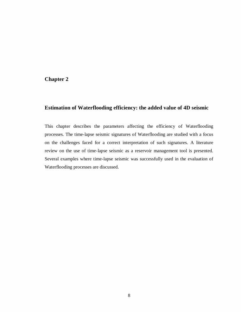
volume (Figure 2.1). It is worth noting however that most of the oil fields selected for

development by Waterflooding have low oil viscosity, generally associated with a

favourable mobility ratio (M <1) (Dake, 2001). The effects of the mobility ratio of the

efficiency of water-oil displacement are visible only on the microscopic, one

dimensional scale. In the case of Waterflooding of a reservoir, one must also consider

the heterogeneity and gravity effects on the overall flooding efficiency.

Figure 2.1: Effects of mobility ratio on water-oil displacement.

2.1.2 Reservoir heterogeneities and gravity:

In reservoir sections, scale, gravity and heterogeneity are closely interrelated and they

have a combined influence on the Waterflooding efficiency. The gravity effect is always

combined with the heterogeneity effects to produce a stable or a non-stable water-oil

displacement. The mobility ratio influence is swamped but it can indicate the ease with

which water can be injected into a reservoir.

11

In assessing the heterogeneity of the reservoir, the most significant parameter to consider

is the permeability and in particular its degree of variation across the reservoir section

(Willhite, 1986). This is due to the fact that permeability can vary by several orders of

magnitude within a matter of a few feet which makes its influence overshadow the

influences of other parameters like porosity and water saturation. In the case of

coarsening upward of the permeability across the reservoir section, a piston-like

displacement may occur provided the cross-flow of fluids under the influence of gravity

is not prohibited (vertical equilibrium conditions). In this situation, the heterogeneity of

the reservoir (mainly controlled by the vertical permeability distribution) and the gravity

complement each other and can produce a piston-like displacement even for an

unfavourable mobility ratio. In fact, as the water enters the structure, it moves faster in

the higher permeability top layers according to Darcy’s law. But as the water progresses

away from the well, the viscous driving forces from the injection pumping decrease and

at some point diminish so that gravity will govern. The water then slumps to the base

and the overall effect is the development of a sharp front and perfect piston-like

displacement across the reservoir section.

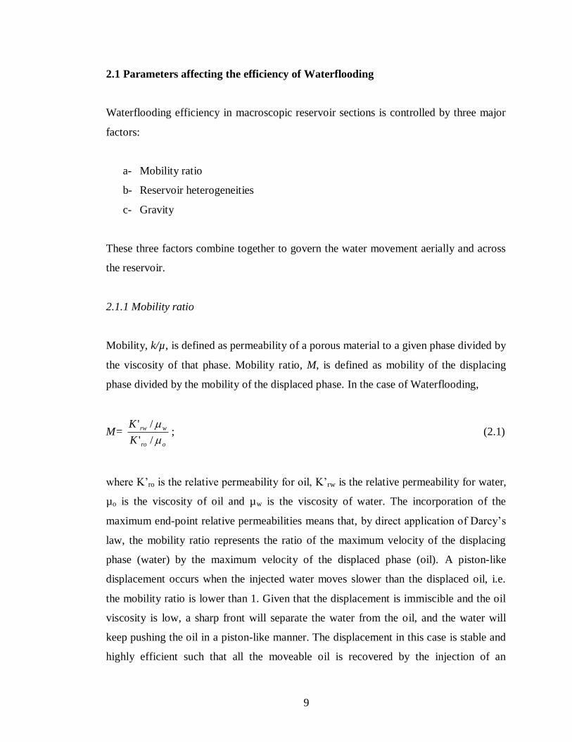
If the higher permeability is in the bottom of the reservoir (coarsening downward), the

gravity effect will be intensified and an unfavourable displacement will happen leading

to the necessity to circulate huge amount of water in order to move the oil in place, even

with a mobility ratio less than unity (Figure 2.2).

12

Figure 2.2: Effect of permeability distribution of Waterflooding efficiency.

2.2 Time-lapse seismic signature of Waterflooding

2.2.1 Theoretical background

Our study focused on two phases (oil and water) systems, where water is injected into

the reservoir to displace the oil towards the producers. In this case the waterfront is the

oil-water contact so both terms are used interchangeably across the whole chapter. In the

case where a natural aquifer is present in the reservoir, the oil/water contact will be

called original oil/water contact (OOWC) for clarity purposes. The identification of

OWC movement from 4D seismic was one of the earliest practical applications of this

technique. Even at the qualitative stage, it brought valuable information revealing

unswept areas, or flow barriers that cannot be determined without dynamic seismic

information. The successful identification of contact movement that can be obtained

from the simple subtraction of base and monitor surveys depend among other factors on

the signal to noise ratio or tuning that is why other seismic attributes are often used to

emphasize the contact variation that eventually cannot be observed using simple

13

amplitude subtraction. Inverted acoustic impedance maps and cross-sections are

powerful tools for the identification of fluids contact and are widely used as the

preferred 4D seismic attribute to extract the OWC movement (Khahar et al., 2006).

Complex attributes were proven useful in the identification of such contacts and their

movement across the reservoir (Schinelli, 2006).

The identification of OWC movement from time-lapse seismic is not only constrained

by the seismic acquisition parameters (S/N ratio, source wavelet, etc.) but also by the

inherent reservoir geology such as rock petrophysical and elastic parameters,

heterogeneities, etc. The fluids characteristics, mainly the acoustic contrast between the

displacing (water) and displaced (oil) fluids, will also determine whether any fluids

substitution is seismically detectable. This means that not every reservoir undergoing

Waterflooding as a secondary recovery technique is a suitable candidate for time-lapse

seismic Waterflooding. Investigating the feasibility of such monitoring is beyond the

scope of this thesis (Wang et al., 1991). Our work will focus on turbidite reservoirs

where several successes were reported (MacBeth et al., 2005).

Interpretation of the 4D signature of Waterflooding gives information about

swept/unswept areas in the reservoir and the location of the OWC at the time of the

seismic acquisition of the monitor survey. However in order for this interpretation to be

meaningful, the complex nature of this signature has to be understood. In fact, during

Waterflooding, several dynamic reservoir properties are changing simultaneously.

Laboratory investigations and theoretical analysis have shown that the velocities and

density of rocks are affected by changes in the temperature, composition, density and

pressure of pore fluids (Wang and Nur, 1986; Wang et al., 1990; Batzle and Wang,

1992). The fluid substitution that occurs during the production of hydrocarbon reservoirs

changes the compressibility of the pore fluids, thus changing the velocity of the overall

rock. In Waterflooding, the injected water decreases the overall compressibility of the

rock, raising the velocity. Many investigations in the laboratory have shown that pore

pressure changes affect the seismic velocity (Wyllie et al., 1958; Han et al., 1986;

Freund, 1992). During production, fluid injection will increase pore pressure, decreasing

14

the effective stress and lowering velocities. Hydrocarbon extraction can cause a decline

in pore pressure, which results in increasing velocity until the bubble point is reached,

after which gas comes out of solution, decreasing the seismic velocity.

Consider a reservoir in which only two phases, oil and water, are present; and where the

oil is assumed to be undersaturated and hence the reservoir pressure is above bubble

point. Generally, the seismic attribute A, computed at the top reservoir, base or some

intra-reservoir horizon, is dependent on the reservoir thickness (τ), lithology (L),

porosity (Φ), reservoir pressure (P) and oil saturation (So) (MacBeth et al., 2004)

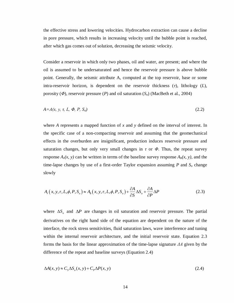
A=A(x, y, τ, L, Φ, P, So) (2.2)

where A represents a mapped function of x and y defined on the interval of interest. In

the specific case of a non-compacting reservoir and assuming that the geomechanical

effects in the overburden are insignificant, production induces reservoir pressure and

saturation changes, but only very small changes in τ or Φ. Thus, the repeat survey

response Ar(x, y) can be written in terms of the baseline survey response Ab(x, y), and the

time-lapse changes by use of a first-order Taylor expansion assuming P and So change

slowly

, , , , , , , , , , , ,r o b o o

A AA x y L P S A x y L P S S P

S P

(2.3)

where oS and P are changes in oil saturation and reservoir pressure. The partial

derivatives on the right hand side of the equation are dependent on the nature of the

interface, the rock stress sensitivities, fluid saturation laws, wave interference and tuning

within the internal reservoir architecture, and the initial reservoir state. Equation 2.3

forms the basis for the linear approximation of the time-lapse signature ΔA given by the

difference of the repeat and baseline surveys (Equation 2.4)

( , ) ( , ) ( , )S o PA x y C S x y C P x y (2.4)

15

where CS and CP are constants to be determined, and ΔSo and ΔP are average oil

saturation and fluid pressure. Initially, the coefficients CS and CP are considered to be

invariant across the reservoir. This imposes the condition of a weak facies and porosity

variation across the reservoir, and invariant cap-rock properties. In addition, the

velocities changes in the cap rock due to stress changes are considerable insignificant.

This could not be the case in some reservoirs or areas of the reservoir with considerable

change in stress in the overburden.

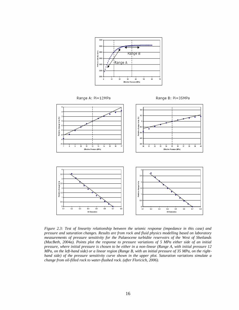
The above equation holds, provided that changes in pressure and saturation are not

unreasonably large. Figure 2.3 gives some idea of the validity of the assumptions upon

which it is based. In several oil reservoirs, the pressure fluctuation is held at a small

percentage of the initial pressure, as it is generally not in the best economic interests to

do otherwise. Typically, a reservoir may deplete by up to 5 to 10 MPa (725 to 1450 psi),

while during injection (with the exception of the immediate vicinity of the well) the

pressure might fluctuate by no more than 10 MPa (1450 psi). The change of pressure

also depends on proximity to the bubble point, and good management practice tends to

ensure pressure maintenance a few MPa above the bubble point. The linear

approximation of amplitude versus pressure will hold with a small overall percentage

error for pressure changes of 5 to 10 MPa. Typically, in an oil-water system, for

example, oil saturation will change from 1−Swc (approximately 60-85%) to Sor

(approximately 15-25%). Calculations, however, have shown that even under these

situations the linearity assumption appears adequate as a working rule (Figure 2.3).

16

Figure 2.3: Test of linearity relationship between the seismic response (impedance in this case) and

pressure and saturation changes. Results are from rock and fluid physics modelling based on laboratory

measurements of pressure sensitivity for the Palaeocene turbidite reservoirs of the West of Shetlands

(MacBeth, 2004a). Points plot the response to pressure variations of 5 MPa either side of an initial

pressure, where initial pressure is chosen to be either in a non-linear (Range A, with initial pressure 12

MPa, on the left-hand side) or a linear region (Range B, with an initial pressure of 35 MPa, on the right-

hand side) of the pressure sensitivity curve shown in the upper plot. Saturation variations simulate a

change from oil-filled rock to water-flushed rock. (after Floricich, 2006).

17

2.2.2 Overlapping of Pressure and saturation change effects

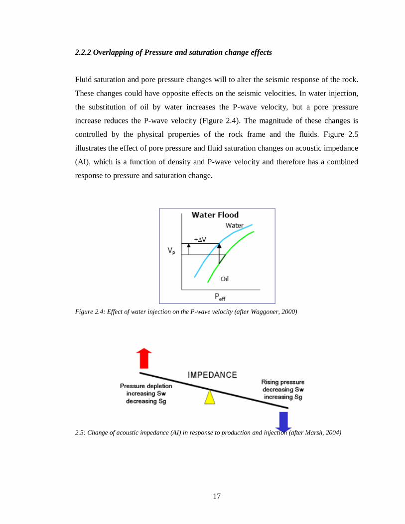
Fluid saturation and pore pressure changes will to alter the seismic response of the rock.

These changes could have opposite effects on the seismic velocities. In water injection,

the substitution of oil by water increases the P-wave velocity, but a pore pressure

increase reduces the P-wave velocity (Figure 2.4). The magnitude of these changes is

controlled by the physical properties of the rock frame and the fluids. Figure 2.5

illustrates the effect of pore pressure and fluid saturation changes on acoustic impedance

(AI), which is a function of density and P-wave velocity and therefore has a combined

response to pressure and saturation change.

Figure 2.4: Effect of water injection on the P-wave velocity (after Waggoner, 2000)

2.5: Change of acoustic impedance (AI) in response to production and injection (after Marsh, 2004)

18

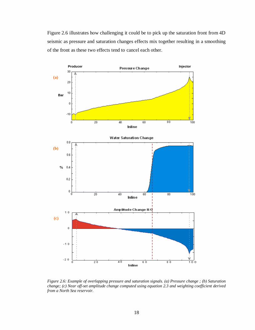
Figure 2.6 illustrates how challenging it could be to pick up the saturation front from 4D

seismic as pressure and saturation changes effects mix together resulting in a smoothing

of the front as these two effects tend to cancel each other.

Producer Injector

Bar

%

Figure 2.6: Example of overlapping pressure and saturation signals. (a) Pressure change ; (b) Saturation

change; (c) Near off-set amplitude change computed using equation 2.3 and weighting coefficient derived from a North Sea reservoir.

(a)

(b)

(c)

19

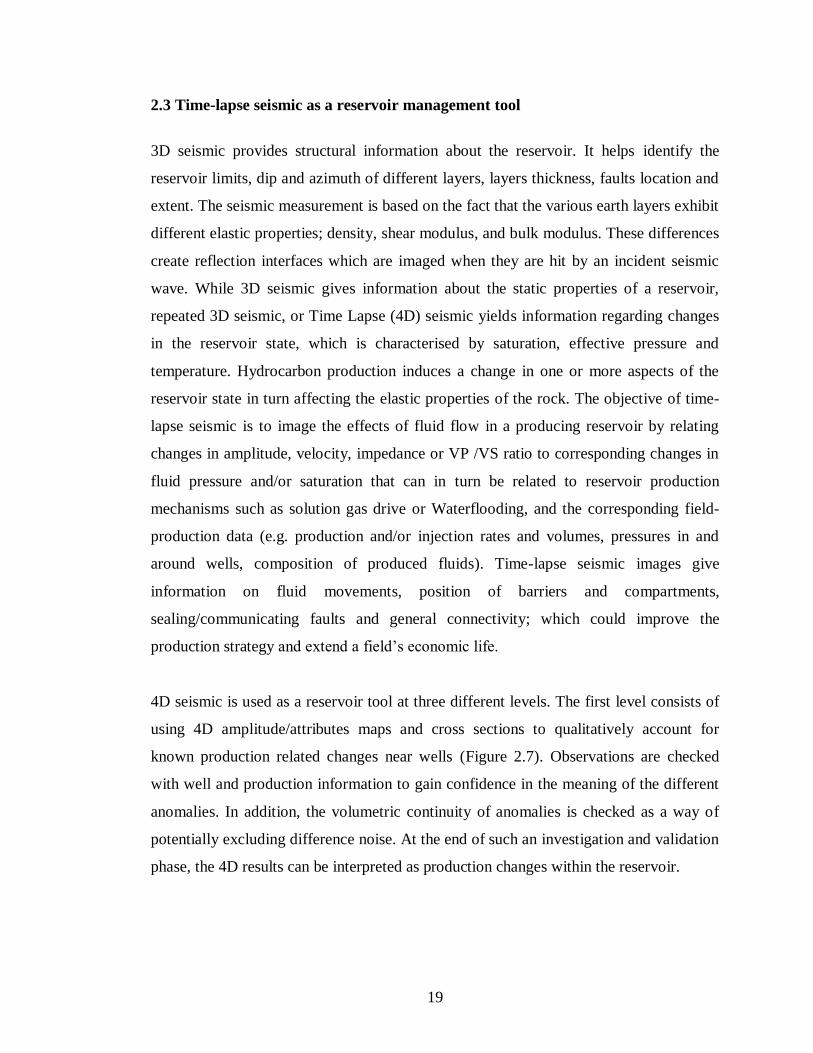
2.3 Time-lapse seismic as a reservoir management tool

3D seismic provides structural information about the reservoir. It helps identify the

reservoir limits, dip and azimuth of different layers, layers thickness, faults location and

extent. The seismic measurement is based on the fact that the various earth layers exhibit

different elastic properties; density, shear modulus, and bulk modulus. These differences

create reflection interfaces which are imaged when they are hit by an incident seismic

wave. While 3D seismic gives information about the static properties of a reservoir,

repeated 3D seismic, or Time Lapse (4D) seismic yields information regarding changes

in the reservoir state, which is characterised by saturation, effective pressure and

temperature. Hydrocarbon production induces a change in one or more aspects of the

reservoir state in turn affecting the elastic properties of the rock. The objective of time-

lapse seismic is to image the effects of fluid flow in a producing reservoir by relating

changes in amplitude, velocity, impedance or VP /VS ratio to corresponding changes in

fluid pressure and/or saturation that can in turn be related to reservoir production

mechanisms such as solution gas drive or Waterflooding, and the corresponding field-

production data (e.g. production and/or injection rates and volumes, pressures in and

around wells, composition of produced fluids). Time-lapse seismic images give

information on fluid movements, position of barriers and compartments,

sealing/communicating faults and general connectivity; which could improve the

production strategy and extend a field’s economic life.

4D seismic is used as a reservoir tool at three different levels. The first level consists of

using 4D amplitude/attributes maps and cross sections to qualitatively account for

known production related changes near wells (Figure 2.7). Observations are checked

with well and production information to gain confidence in the meaning of the different

anomalies. In addition, the volumetric continuity of anomalies is checked as a way of

potentially excluding difference noise. At the end of such an investigation and validation

phase, the 4D results can be interpreted as production changes within the reservoir.

20

Figure 2.7: Conventional Time-Lapse seismic interpretation, (after Floricich, 2006)

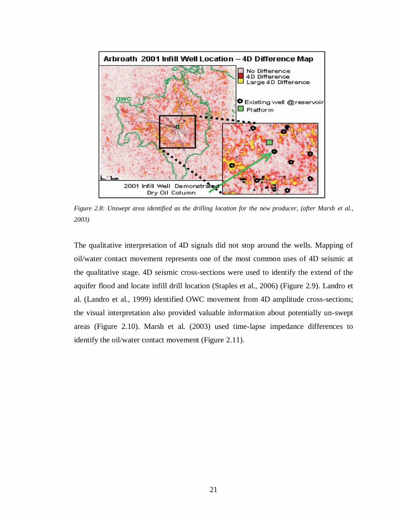
Marsh et al. (2003) identified unswept areas for an infill producer drilling location in the

Arbroath field in the North Sea. This simple evaluation involved identifying the original

oil–water contact (OWC) on seismic data and screening 4D difference sections to

identify those areas where the contact appeared to have moved. A seismic attribute map

was then calculated which showed up these areas which were cross-matched to water-

cut development in the existing wells (Figure 2.8).

The map indicated that the proposed infill location south of the platform did not seem to

have suffered visible water migration. The size and shape of this unswept area supported

that postulated by the original reservoir simulation modeling. The producer was drilled

in mid-2001 and came on at a good oil rate and negligible water-cut.

21

Figure 2.8: Unswept area identified as the drilling location for the new producer, (after Marsh et al.,

2003)

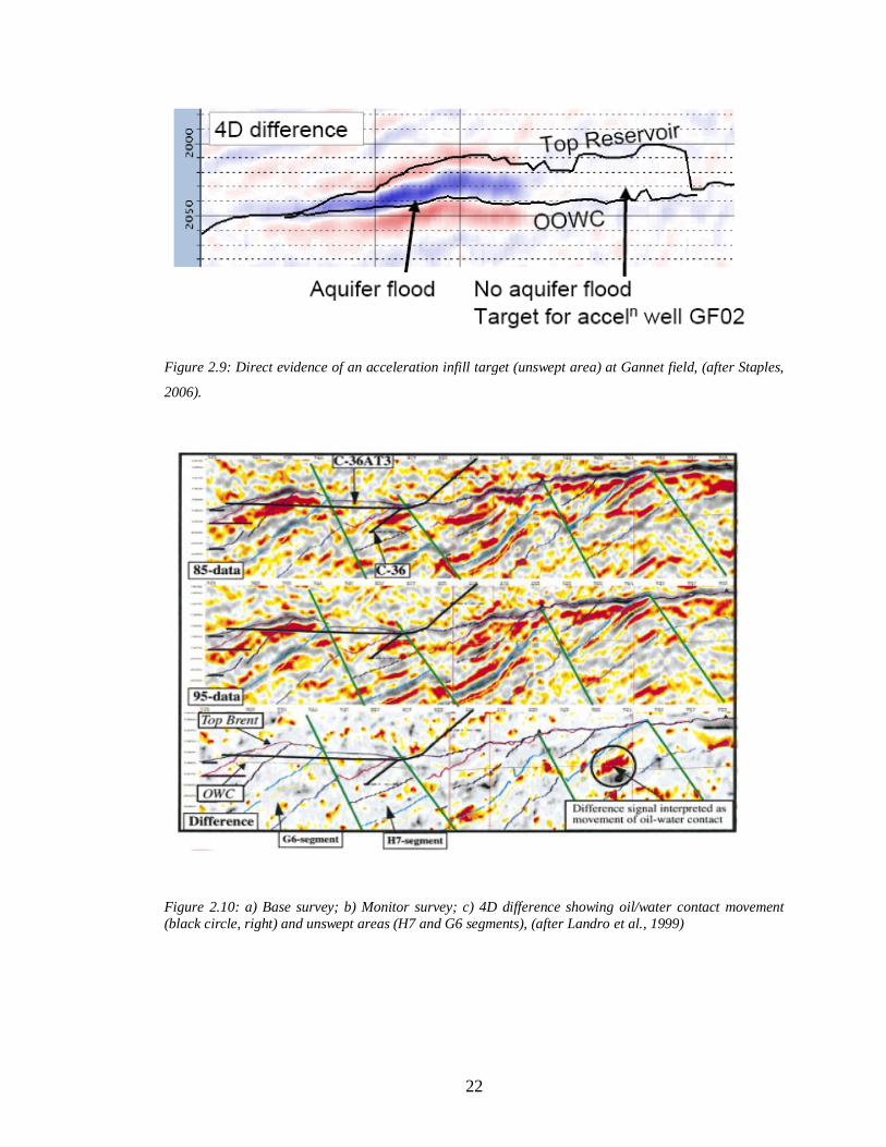
The qualitative interpretation of 4D signals did not stop around the wells. Mapping of

oil/water contact movement represents one of the most common uses of 4D seismic at

the qualitative stage. 4D seismic cross-sections were used to identify the extend of the

aquifer flood and locate infill drill location (Staples et al., 2006) (Figure 2.9). Landro et

al. (Landro et al., 1999) identified OWC movement from 4D amplitude cross-sections;

the visual interpretation also provided valuable information about potentially un-swept

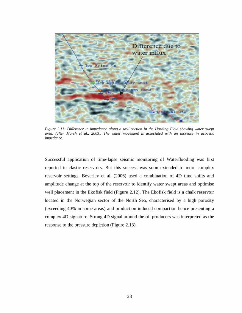
areas (Figure 2.10). Marsh et al. (2003) used time-lapse impedance differences to

identify the oil/water contact movement (Figure 2.11).

22

Figure 2.9: Direct evidence of an acceleration infill target (unswept area) at Gannet field, (after Staples,

2006).

Figure 2.10: a) Base survey; b) Monitor survey; c) 4D difference showing oil/water contact movement

(black circle, right) and unswept areas (H7 and G6 segments), (after Landro et al., 1999)

23

Figure 2.11: Difference in impedance along a well section in the Harding Field showing water swept area, (after Marsh et al., 2003). The water movement is associated with an increase in acoustic

impedance.

Successful application of time-lapse seismic monitoring of Waterflooding was first

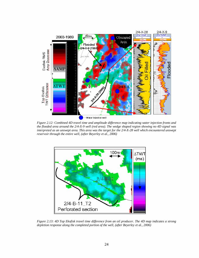
reported in clastic reservoirs. But this success was soon extended to more complex

reservoir settings. Beyerley et al. (2006) used a combination of 4D time shifts and

amplitude change at the top of the reservoir to identify water swept areas and optimise

well placement in the Ekofisk field (Figure 2.12). The Ekofisk field is a chalk reservoir

located in the Norwegian sector of the North Sea, characterised by a high porosity

(exceeding 40% in some areas) and production induced compaction hence presenting a

complex 4D signature. Strong 4D signal around the oil producers was interpreted as the

response to the pressure depletion (Figure 2.13).

24

Figure 2.12: Combined 4D travel time and amplitude difference map indicating water injection fronts and

the flooded area around the 2/4-X-9 well (red area). The wedge shaped region showing no 4D signal was

interpreted as an unswept area. This area was the target for the 2/4-X-28 well which encountered unswept reservoir through the entire well, (after Beyerley et al., 2006)

Figure 2.13: 4D Top Ekofisk travel time difference from an oil producer. The 4D map indicates a strong

depletion response along the completed portion of the well, (after Beyerley et al., 2006)

25

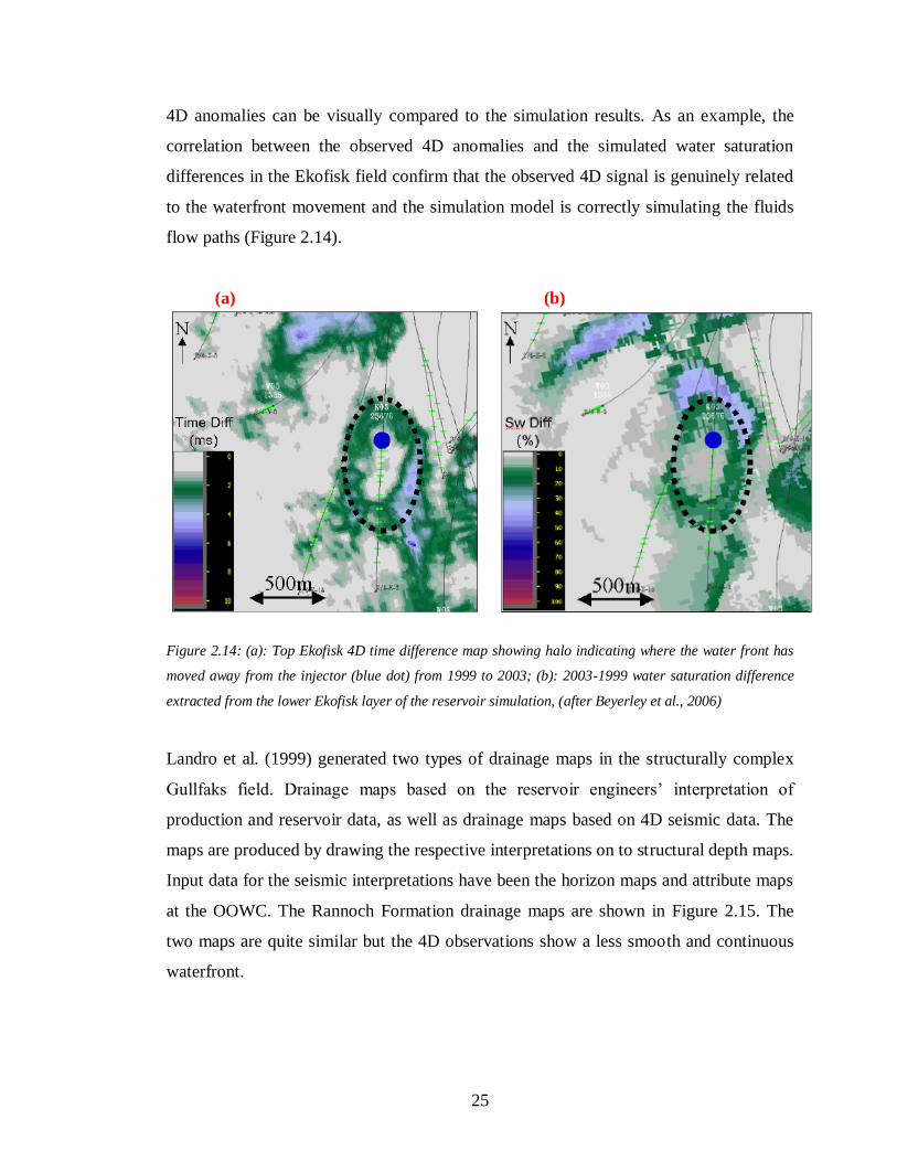
4D anomalies can be visually compared to the simulation results. As an example, the

correlation between the observed 4D anomalies and the simulated water saturation

differences in the Ekofisk field confirm that the observed 4D signal is genuinely related

to the waterfront movement and the simulation model is correctly simulating the fluids

flow paths (Figure 2.14).

(a) (b)

Figure 2.14: (a): Top Ekofisk 4D time difference map showing halo indicating where the water front has

moved away from the injector (blue dot) from 1999 to 2003; (b): 2003-1999 water saturation difference

extracted from the lower Ekofisk layer of the reservoir simulation, (after Beyerley et al., 2006)

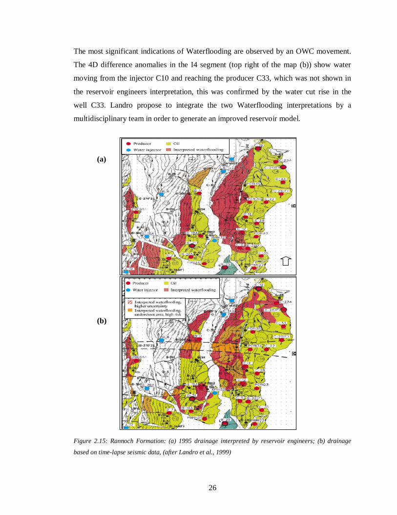
Landro et al. (1999) generated two types of drainage maps in the structurally complex

Gullfaks field. Drainage maps based on the reservoir engineers’ interpretation of

production and reservoir data, as well as drainage maps based on 4D seismic data. The

maps are produced by drawing the respective interpretations on to structural depth maps.

Input data for the seismic interpretations have been the horizon maps and attribute maps

at the OOWC. The Rannoch Formation drainage maps are shown in Figure 2.15. The

two maps are quite similar but the 4D observations show a less smooth and continuous

waterfront.

26

The most significant indications of Waterflooding are observed by an OWC movement.

The 4D difference anomalies in the I4 segment (top right of the map (b)) show water

moving from the injector C10 and reaching the producer C33, which was not shown in

the reservoir engineers interpretation, this was confirmed by the water cut rise in the

well C33. Landro propose to integrate the two Waterflooding interpretations by a

multidisciplinary team in order to generate an improved reservoir model.

(a)

(b)

Figure 2.15: Rannoch Formation: (a) 1995 drainage interpreted by reservoir engineers; (b) drainage

based on time-lapse seismic data, (after Landro et al., 1999)

27

It is common in reservoir simulation that equiprobable model realizations are generated.

Several of these models can be history matched to production data with the same level of

accuracy. Comparing interpreted time-lapse changes against predictions from multiple

models can lead to the exclusion of some of the models that do not match the 4D

anomalies and help choose the best model for reservoir management (Figure 2.16).

Figure 2.16: Simulation model selection constrained by 4D seismic, (after Floricich, 2006)

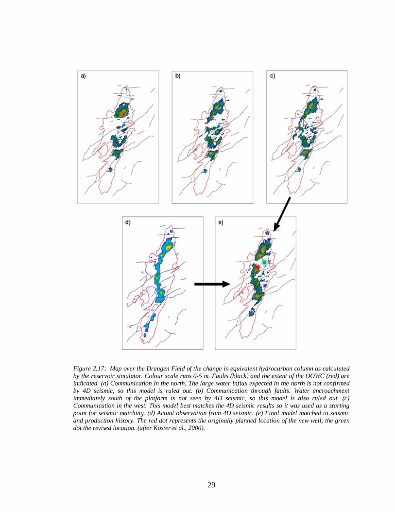
Koster et al. (2000) showed an example for the Draugen Field, in the North Sea. In the

Draugen field, water injectors at the north and south end of a low-relief anticline

structure push oil toward the central producers. The lack of wells between the producers

and the injectors resulted in a considerable uncertainty in reservoir properties, and

several reservoir simulation models were built using different communication paths

between the aquifer and the reservoir. All versions of the reservoir model had assumed

that water movement would occur along both flanks of the field (Figure 2.17). These

models can all be matched to the production data. However, these models have

significantly different forecast production profiles for the field. Therefore, knowledge of

the true communication path would allow optimization of the production strategy. The

communication path also has a significant impact on the location of the waterfront

28

within the reservoir. Figure 2.17d shows a map of the difference in amplitudes at a

picked event. This clearly shows where water has replaced oil, giving a snapshot of the

waterflood situation away from the wells, and therefore resolving many uncertainties.

The measured 4D shows the injected water moving along the western flank, with no

displacement on the eastern flank. Also, a northern fault is clearly shown to be sealing

during the production time. The reservoir model that was closest to the 4D result was

selected for reservoir management purposes.

Forward rock physics modelling is used to create synthetic seismic from the simulation

results. The comparison of the real 4D signal with the synthetic one can help ascertain

the robustness of the simulation model and assist in the interpretation of the real time-

lapse seismic signal. Staples et al. (2006) used forward modelling in the Gannet C field

to improve history matching, with a manual history matching cycle including updates to

the static model (Figure 2.18). This technique is also used to reduce the non-uniqueness

of reservoir flow simulation results. In fact, reservoir simulation can yield multiple

equiprobable realisations which honour the historical production data. Lumley et al.

(1998) showed an example where forward rock physics modelling helped choose the

best model that matched both production data and 4D seismic data (Figure 2.19).

Other examples summarizing semi-quantitative integration of time-lapse seismic and

production data can be found in Al-Najjar et al. (1999); Waggoner (2001); Staples et al.

(2002) and Marsh et al. (2003). A review of these articles shows that the comparison of

the 4D signature with the predicted output from a simulation model has been successful

at locating dynamic barriers, varying fault transmissibility (seal or no seal), altering

aquifer connectivity, identifying injected water slumping and running on top of shales

(gas running under shales; identification of thief zones), and STOIIP adjustment. This

process is, however, non-unique and not strictly quantitative.

29

Figure 2.17: Map over the Draugen Field of the change in equivalent hydrocarbon column as calculated

by the reservoir simulator. Colour scale runs 0-5 m. Faults (black) and the extent of the OOWC (red) are indicated. (a) Communication in the north. The large water influx expected in the north is not confirmed

by 4D seismic, so this model is ruled out. (b) Communication through faults. Water encroachment

immediately south of the platform is not seen by 4D seismic, so this model is also ruled out. (c)

Communication in the west. This model best matches the 4D seismic results so it was used as a starting

point for seismic matching. (d) Actual observation from 4D seismic. (e) Final model matched to seismic

and production history. The red dot represents the originally planned location of the new well, the green

dot the revised location. (after Koster et al., 2000).

30

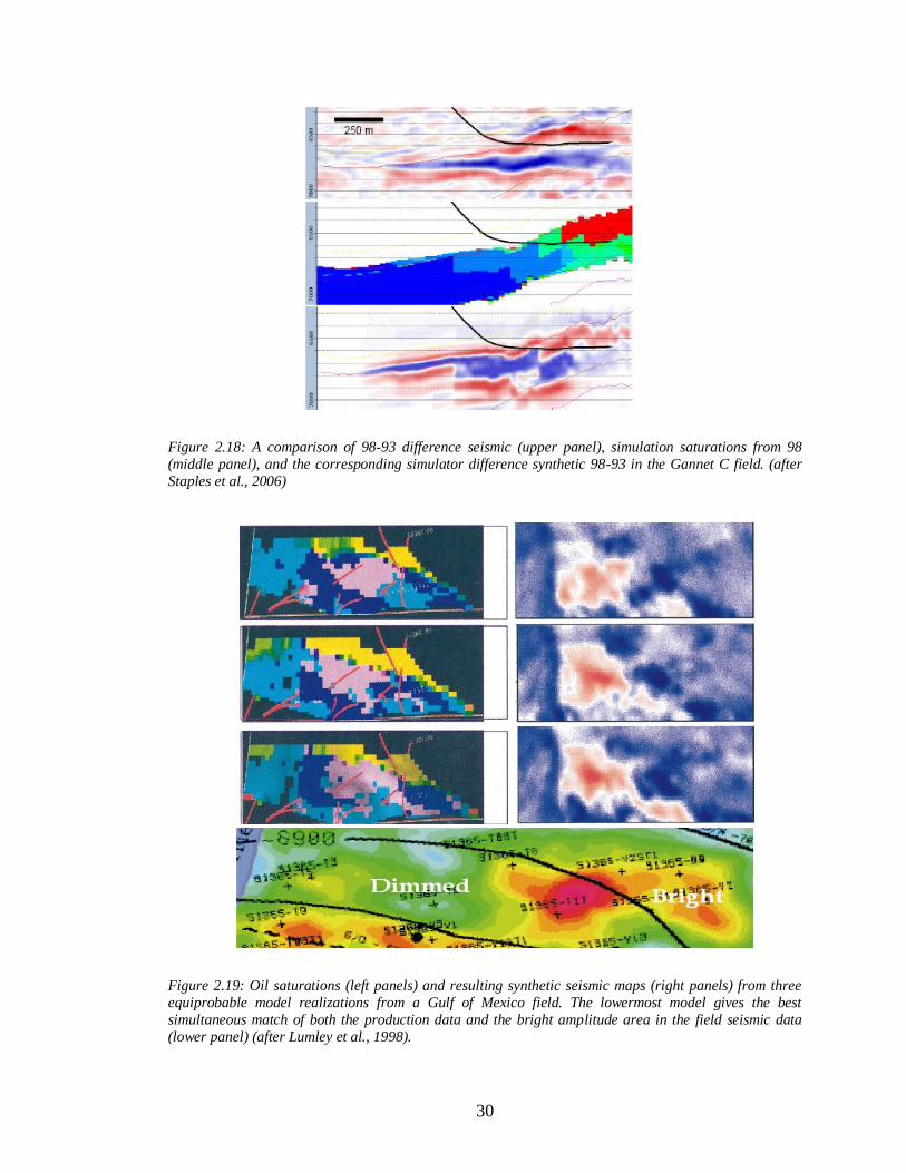
Figure 2.18: A comparison of 98-93 difference seismic (upper panel), simulation saturations from 98

(middle panel), and the corresponding simulator difference synthetic 98-93 in the Gannet C field. (after

Staples et al., 2006)

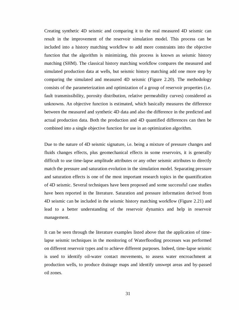
Figure 2.19: Oil saturations (left panels) and resulting synthetic seismic maps (right panels) from three

equiprobable model realizations from a Gulf of Mexico field. The lowermost model gives the best

simultaneous match of both the production data and the bright amplitude area in the field seismic data

(lower panel) (after Lumley et al., 1998).

31

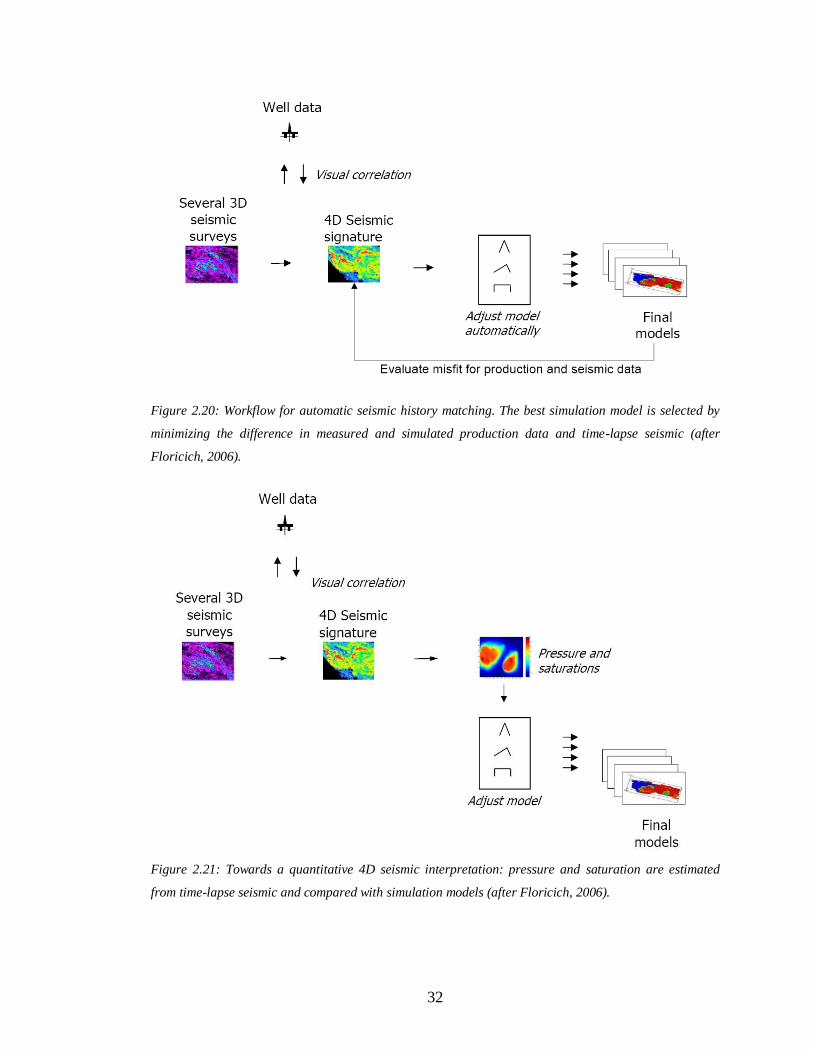
Creating synthetic 4D seismic and comparing it to the real measured 4D seismic can

result in the improvement of the reservoir simulation model. This process can be

included into a history matching workflow to add more constraints into the objective

function that the algorithm is minimizing, this process is known as seismic history

matching (SHM). The classical history matching workflow compares the measured and

simulated production data at wells, but seismic history matching add one more step by

comparing the simulated and measured 4D seismic (Figure 2.20). The methodology

consists of the parameterization and optimization of a group of reservoir properties (i.e.

fault transmissibility, porosity distribution, relative permeability curves) considered as

unknowns. An objective function is estimated, which basically measures the difference

between the measured and synthetic 4D data and also the difference in the predicted and

actual production data. Both the production and 4D quantified differences can then be

combined into a single objective function for use in an optimization algorithm.

Due to the nature of 4D seismic signature, i.e. being a mixture of pressure changes and

fluids changes effects, plus geomechanical effects in some reservoirs, it is generally

difficult to use time-lapse amplitude attributes or any other seismic attributes to directly

match the pressure and saturation evolution in the simulation model. Separating pressure

and saturation effects is one of the most important research topics in the quantification

of 4D seismic. Several techniques have been proposed and some successful case studies

have been reported in the literature. Saturation and pressure information derived from

4D seismic can be included in the seismic history matching workflow (Figure 2.21) and

lead to a better understanding of the reservoir dynamics and help in reservoir

management.

It can be seen through the literature examples listed above that the application of time-

lapse seismic techniques in the monitoring of Waterflooding processes was performed

on different reservoir types and to achieve different purposes. Indeed, time-lapse seismic

is used to identify oil-water contact movements, to assess water encroachment at

production wells, to produce drainage maps and identify unswept areas and by-passed

oil zones.

32

Figure 2.20: Workflow for automatic seismic history matching. The best simulation model is selected by

minimizing the difference in measured and simulated production data and time-lapse seismic (after

Floricich, 2006).

Figure 2.21: Towards a quantitative 4D seismic interpretation: pressure and saturation are estimated

from time-lapse seismic and compared with simulation models (after Floricich, 2006).

33

Information derived from time-lapse seismic data interpretation can therefore be used at

different stages of the reservoir management process. It can carry direct information

about the reservoir state at a specific production time, i.e. fluids contacts, unswept zones,

pressure variations. But it also, if correctly interpreted, gives valuable information about

the reservoir inherent geological complexities and variations.

Waterflooding monitoring using the time-lapse seismic techniques can therefore be seen

on various levels: from the qualitative assessment of fluids contacts locations and

flooded zones identification, to semi-qualitative drainage maps to be calibrated with

production data and compared to reservoir simulation outputs, to quantitative maps of

separate estimations of pressure and saturation changes within the reservoir. This in turn

provides information about reservoir compartmentalization and connectivity and the

sealing nature of internal faults and fractures.

Changes in the reservoir conditions inevitably result in changes in the rock’s seismic

properties. Whether these changes are detectable using 3D and 4D seismic imaging

depends on several factors (oil gravity, substituting-fluids/substituted-fluid acoustic

contrast, reservoir geology, seismic acquisition parameters, etc). Detectability is the

ability to detect changes in the seismic response due to alterations in pressure and

saturation during production. An appropriate rock physics model is critical to assessing

detectability (Behrens et al., 2002).

Time-lapse seismic studies are tied to the particular production scenario in a given

reservoir, whether being a primary or a secondary production mechanism. Gassmann

(Gassmann, 1951) equations, whose applicability in porous media is limited to

homogeneous isotropic rocks under isobaric conditions, are frequently used to link the

seismic response to changes in reservoir properties. A typical form for Gassmann

equation is the following:

34

2

0

2

0 0

1

1

dry

sat dry

dry

fluid

K

KK K

k

K K K

sat dry

where Ksat is the saturated-rock modulus, Kdry the frame (dry) bulk modulus, while K0

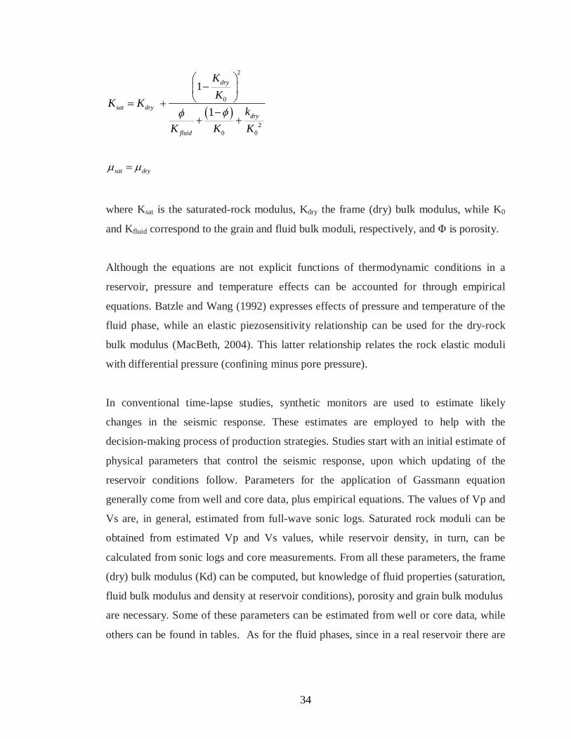
and Kfluid correspond to the grain and fluid bulk moduli, respectively, and Φ is porosity.

Although the equations are not explicit functions of thermodynamic conditions in a

reservoir, pressure and temperature effects can be accounted for through empirical

equations. Batzle and Wang (1992) expresses effects of pressure and temperature of the

fluid phase, while an elastic piezosensitivity relationship can be used for the dry-rock

bulk modulus (MacBeth, 2004). This latter relationship relates the rock elastic moduli

with differential pressure (confining minus pore pressure).

In conventional time-lapse studies, synthetic monitors are used to estimate likely

changes in the seismic response. These estimates are employed to help with the

decision-making process of production strategies. Studies start with an initial estimate of

physical parameters that control the seismic response, upon which updating of the

reservoir conditions follow. Parameters for the application of Gassmann equation

generally come from well and core data, plus empirical equations. The values of Vp and

Vs are, in general, estimated from full-wave sonic logs. Saturated rock moduli can be

obtained from estimated Vp and Vs values, while reservoir density, in turn, can be

calculated from sonic logs and core measurements. From all these parameters, the frame

(dry) bulk modulus (Kd) can be computed, but knowledge of fluid properties (saturation,

fluid bulk modulus and density at reservoir conditions), porosity and grain bulk modulus

are necessary. Some of these parameters can be estimated from well or core data, while

others can be found in tables. As for the fluid phases, since in a real reservoir there are

35

several fluid components occupying the pore space, it is then necessary to estimate

effective fluid density and bulk modulus.

On the other hand, changes in the seismic response are linked to changes in both the

solid and fluid phases. Therefore, it is important to understand how changes in fluid and

solid properties contribute to those changes in the seismic response, for the different

stress and production scenarios. Our analysis, however, will disregard geomechanical

effects such as subsidence or compaction that can be relevant in certain scenarios of

production, but considers the type of reservoir geology and reservoir dynamics.

2.4 Conclusion

Waterflooding had a tangible impact on oil recovery efficiency by substantially

increasing production from an oil field and delaying abandonment. This success caused

a surge of interest in understanding fluids displacement in porous media and oil/ water

movement within the reservoir rocks. The early techniques to assess Waterflooding

process efficiency were mainly analytical, and generally carried out by engineers. The

advances on computing capabilities, the emergence of new geophysical methods; like

reflection seismic and well logging, and the pressing need to integrate the engineering

domain with the geophysical domain to optimise reservoir management allowed

geoscientists to tackle the issue of Waterflooding through reservoir simulation,

petrophysical modelling and 4D seismic interpretation. Time-lapse seismic proved to be

a powerful tool in the monitoring of Waterflooding. It allowed the identification of un-

swept areas inside the reservoir and the accurate mapping of fluids contacts giving

valuable information as for infill drilling locations and production/injection

optimisation.

The displacement of oil by injected water inevitably causes changes in the reservoir

dynamic properties such as pore pressure and fluids saturation. The interpretation of the

time-lapse seismic signature associated with those changes is not straight forward.

Pressure and saturation changes for example can have opposite effects on seismic

36

amplitude yielding a very weak 4D signature where important dynamics changes

occurred inside the reservoir. Seismic resolution, 4D seismic repeatability and the

quality of the seismic data (i.e. signal to noise ratio) have a major impact on our ability

to correctly extract the needed information for a proper reservoir management.

Waterflooding a geologically complex reservoir adds more challenges as to correctly

identify swept/unswept areas and interpreting fluids contact. The injected water will

flow in some preferential highways dictated by the internal geology of the reservoir and

any flow barriers or compartmentalisation that may be present.

37

Chapter 3

Waterflooding in a clean, thick, and idealised sandstone reservoir:

preliminary study

A series of idealised reservoir models of thick, clean sandstone are built. The reservoir

models present different degrees of geological complexities. Several Waterflooding

scenarios are run; the effects of the geology on the efficiency of Waterflooding are

studied. The results of the petrophysical modelling and the 4D signatures associated with

every Waterflooding scenario and reservoir type are studied.

38

3.1 Introduction

When starting the development of a new hydrocarbon field, 3D seismic data are shot to

help, together with the geological information, delineate the reservoir extent. Appraisal

wells are drilled to collect information about the subsurface geology and fluids content

through well logs, and core data. These data are collected under static conditions; they

do not provide any information about the lateral and vertical pressure communications

which are indispensable in the planning of a successful secondary recovery. In an

onshore environment, production facilities are generally constructed shortly after

discovery of the field; discovery wells are produced at high rates to create a pressure

sink at the well location that will radiate both vertically and laterally throughout the

reservoir. Well tests such as drill stem tests (DST) and repeat formation tester (RFT) are

carried on from the appraisal stage and generally the development plan of the field is

established with a good knowledge of the vertical and lateral communication in the

reservoir. In an offshore environment, however, it is not until the development stage that

such dynamic data can be acquired as no production facilities are present before that

stage so engineers cannot produce from wells for a sufficient time to cause a significant

pressure drop. The important decisions concerning the design of the platform and the

injection and production facilities have to be made before the start of the production

stage. With little or no information about reservoir compartmentalisation, planning of

secondary recovery schemes are mostly predictive and rely heavily on reservoir

simulation. However, simulation models do not necessarily give information about the

reservoir performance; they just reflect the consequences of the input assumptions made

by engineers. Once the development phase starts, the reservoir is finally viewed under

dynamic conditions, and the dynamic data are integrated into the reservoir simulation

model in a history matching process.

The objective of the work in this thesis is to develop a better understanding of fluid flow

in sandstone reservoirs, with a focus on the impact of the geological complexity of the

reservoir and their effect on the resultant 4D seismic signature. The workflow of the

study consists of the creation of 3D reservoir models, running fluid flow simulations,

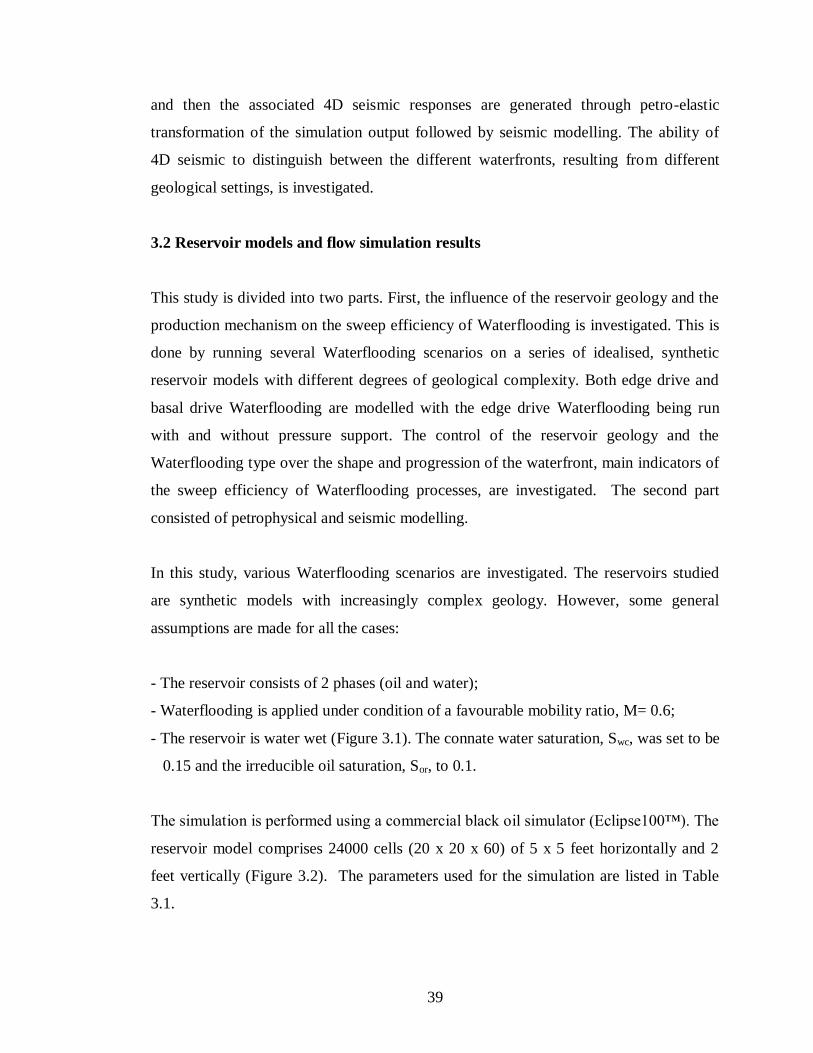
39

and then the associated 4D seismic responses are generated through petro-elastic

transformation of the simulation output followed by seismic modelling. The ability of

4D seismic to distinguish between the different waterfronts, resulting from different

geological settings, is investigated.

3.2 Reservoir models and flow simulation results

This study is divided into two parts. First, the influence of the reservoir geology and the

production mechanism on the sweep efficiency of Waterflooding is investigated. This is

done by running several Waterflooding scenarios on a series of idealised, synthetic

reservoir models with different degrees of geological complexity. Both edge drive and

basal drive Waterflooding are modelled with the edge drive Waterflooding being run

with and without pressure support. The control of the reservoir geology and the

Waterflooding type over the shape and progression of the waterfront, main indicators of

the sweep efficiency of Waterflooding processes, are investigated. The second part

consisted of petrophysical and seismic modelling.

In this study, various Waterflooding scenarios are investigated. The reservoirs studied

are synthetic models with increasingly complex geology. However, some general

assumptions are made for all the cases:

- The reservoir consists of 2 phases (oil and water);

- Waterflooding is applied under condition of a favourable mobility ratio, M= 0.6;

- The reservoir is water wet (Figure 3.1). The connate water saturation, Swc, was set to be

0.15 and the irreducible oil saturation, Sor, to 0.1.

The simulation is performed using a commercial black oil simulator (Eclipse100™). The

reservoir model comprises 24000 cells (20 x 20 x 60) of 5 x 5 feet horizontally and 2

feet vertically (Figure 3.2). The parameters used for the simulation are listed in Table

3.1.

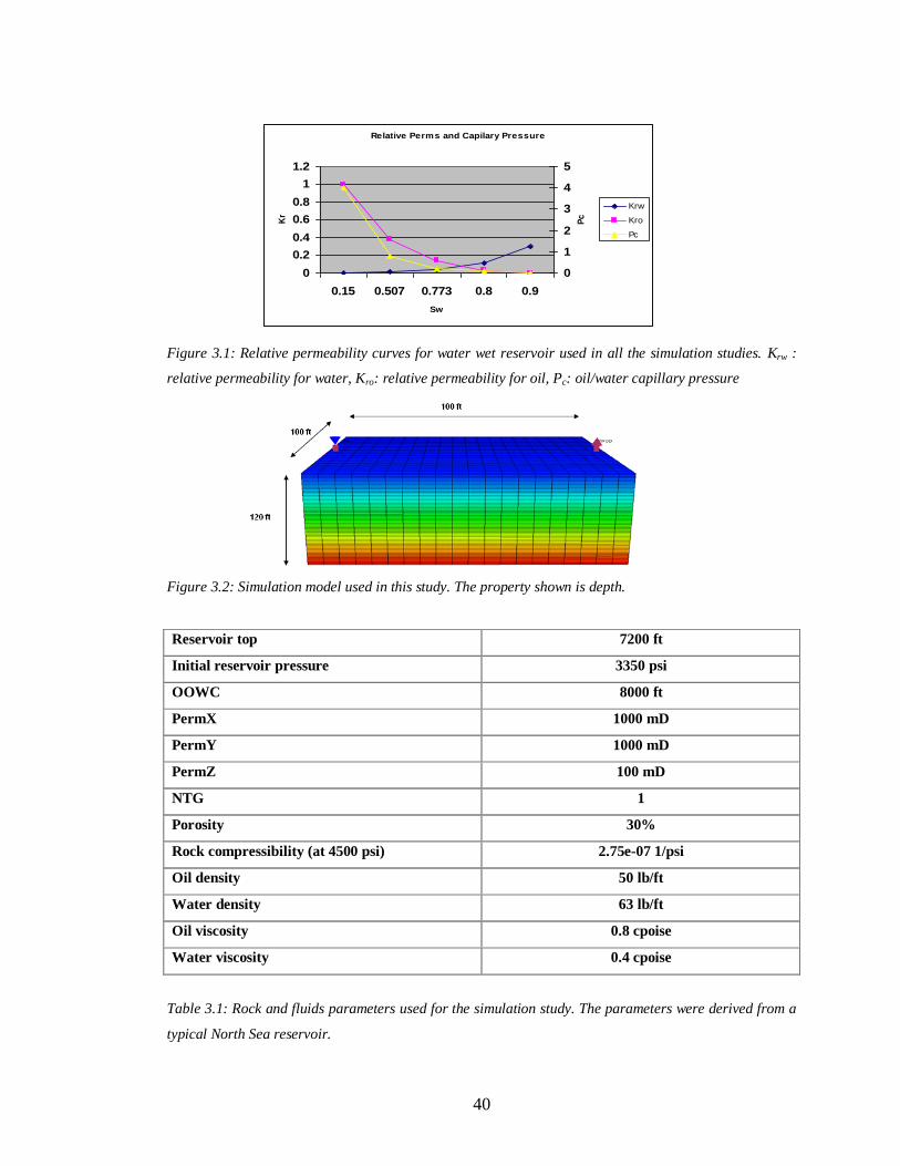
40

Relative Perms and Capilary Pressure

0

0.2

0.4

0.6

0.8

1

1.2

0.15 0.507 0.773 0.8 0.9

Sw

Kr

0

1

2

3

4

5

Pc

Krw

Kro

Pc

Figure 3.1: Relative permeability curves for water wet reservoir used in all the simulation studies. Krw :

relative permeability for water, Kro: relative permeability for oil, Pc: oil/water capillary pressure

Figure 3.2: Simulation model used in this study. The property shown is depth.

Reservoir top 7200 ft

Initial reservoir pressure 3350 psi

OOWC 8000 ft

PermX 1000 mD

PermY 1000 mD

PermZ 100 mD

NTG 1

Porosity 30%

Rock compressibility (at 4500 psi) 2.75e-07 1/psi

Oil density 50 lb/ft

Water density 63 lb/ft

Oil viscosity 0.8 cpoise

Water viscosity 0.4 cpoise

Table 3.1: Rock and fluids parameters used for the simulation study. The parameters were derived from a

typical North Sea reservoir.

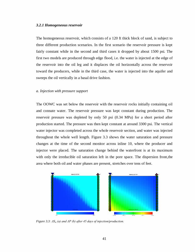
41

3.2.1 Homogeneous reservoir

The homogeneous reservoir, which consists of a 120 ft thick block of sand, is subject to

three different production scenarios. In the first scenario the reservoir pressure is kept

fairly constant while in the second and third cases it dropped by about 1500 psi. The

first two models are produced through edge flood, i.e. the water is injected at the edge of

the reservoir into the oil leg and it displaces the oil horizontally across the reservoir

toward the producers, while in the third case, the water is injected into the aquifer and

sweeps the oil vertically in a basal drive fashion.

a. Injection with pressure support

The OOWC was set below the reservoir with the reservoir rocks initially containing oil

and connate water. The reservoir pressure was kept constant during production. The

reservoir pressure was depleted by only 50 psi (0.34 MPa) for a short period after

production started. The pressure was then kept constant at around 3300 psi. The vertical

water injector was completed across the whole reservoir section, and water was injected

throughout the whole well length. Figure 3.3 shows the water saturation and pressure

changes at the time of the second monitor across inline 10, where the producer and

injector were placed. The saturation change behind the waterfront is at its maximum

with only the irreducible oil saturation left in the pore space. The dispersion front,the

area where both oil and water phases are present, stretches over tens of feet.

Figure 3.3: ΔSw (a) and ΔP (b) after 45 days of injection/production.

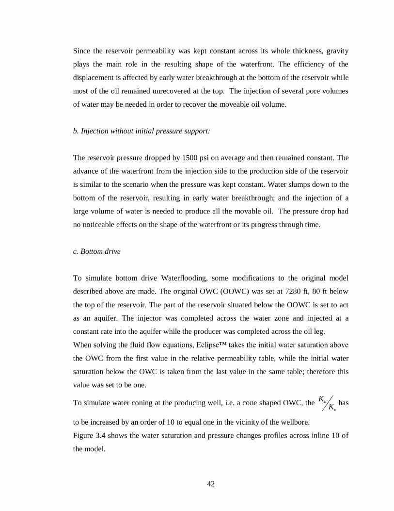
42

Since the reservoir permeability was kept constant across its whole thickness, gravity

plays the main role in the resulting shape of the waterfront. The efficiency of the

displacement is affected by early water breakthrough at the bottom of the reservoir while

most of the oil remained unrecovered at the top. The injection of several pore volumes

of water may be needed in order to recover the moveable oil volume.

b. Injection without initial pressure support:

The reservoir pressure dropped by 1500 psi on average and then remained constant. The

advance of the waterfront from the injection side to the production side of the reservoir

is similar to the scenario when the pressure was kept constant. Water slumps down to the

bottom of the reservoir, resulting in early water breakthrough; and the injection of a

large volume of water is needed to produce all the movable oil. The pressure drop had

no noticeable effects on the shape of the waterfront or its progress through time.

c. Bottom drive

To simulate bottom drive Waterflooding, some modifications to the original model

described above are made. The original OWC (OOWC) was set at 7280 ft, 80 ft below

the top of the reservoir. The part of the reservoir situated below the OOWC is set to act

as an aquifer. The injector was completed across the water zone and injected at a

constant rate into the aquifer while the producer was completed across the oil leg.

When solving the fluid flow equations, Eclipse™ takes the initial water saturation above

the OWC from the first value in the relative permeability table, while the initial water

saturation below the OWC is taken from the last value in the same table; therefore this

value was set to be one.

To simulate water coning at the producing well, i.e. a cone shaped OWC, the h

v

KK

has

to be increased by an order of 10 to equal one in the vicinity of the wellbore.

Figure 3.4 shows the water saturation and pressure changes profiles across inline 10 of

the model.

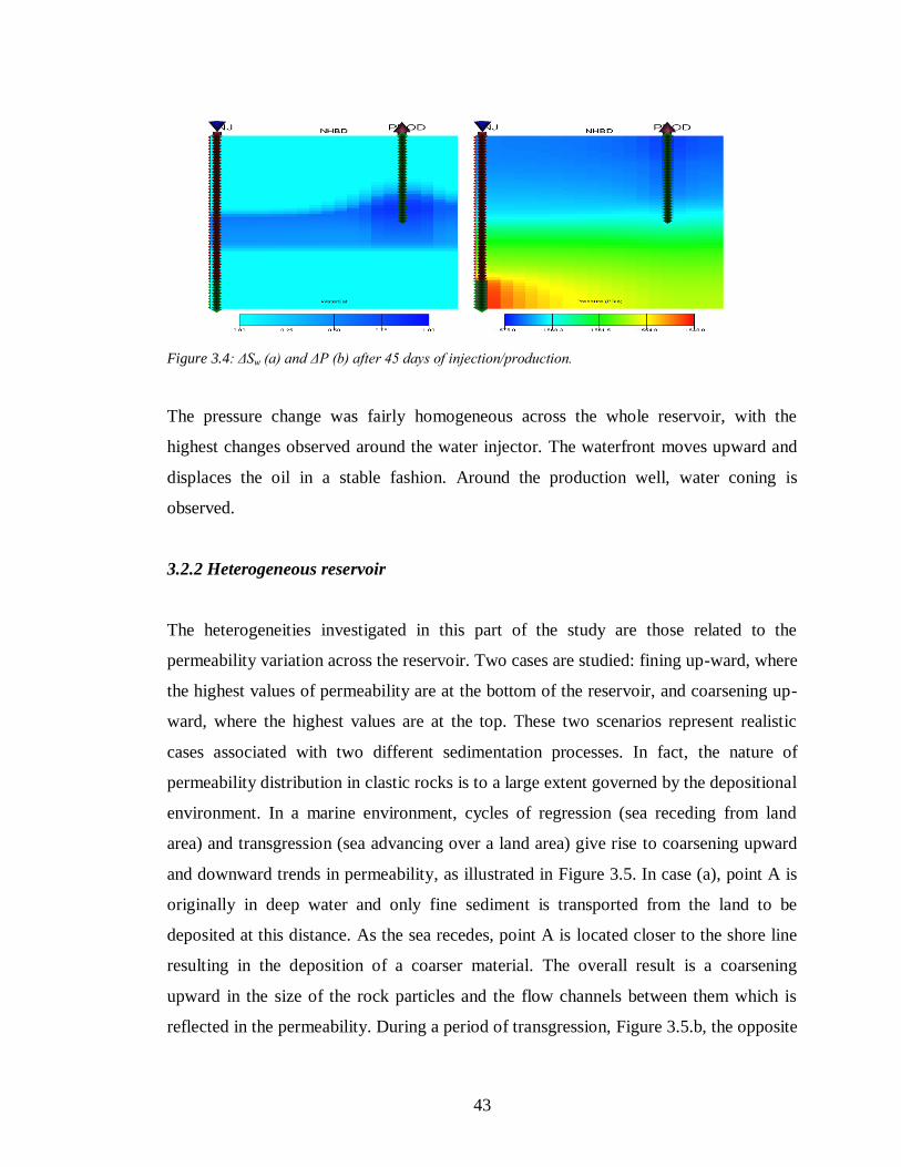
43


The pressure change was fairly homogeneous across the whole reservoir, with the

highest changes observed around the water injector. The waterfront moves upward and

displaces the oil in a stable fashion. Around the production well, water coning is

observed.

3.2.2 Heterogeneous reservoir

The heterogeneities investigated in this part of the study are those related to the

permeability variation across the reservoir. Two cases are studied: fining up-ward, where

the highest values of permeability are at the bottom of the reservoir, and coarsening up-

ward, where the highest values are at the top. These two scenarios represent realistic

cases associated with two different sedimentation processes. In fact, the nature of

permeability distribution in clastic rocks is to a large extent governed by the depositional

environment. In a marine environment, cycles of regression (sea receding from land

area) and transgression (sea advancing over a land area) give rise to coarsening upward

and downward trends in permeability, as illustrated in Figure 3.5. In case (a), point A is

originally in deep water and only fine sediment is transported from the land to be

deposited at this distance. As the sea recedes, point A is located closer to the shore line

resulting in the deposition of a coarser material. The overall result is a coarsening

upward in the size of the rock particles and the flow channels between them which is

reflected in the permeability. During a period of transgression, Figure 3.5.b, the opposite

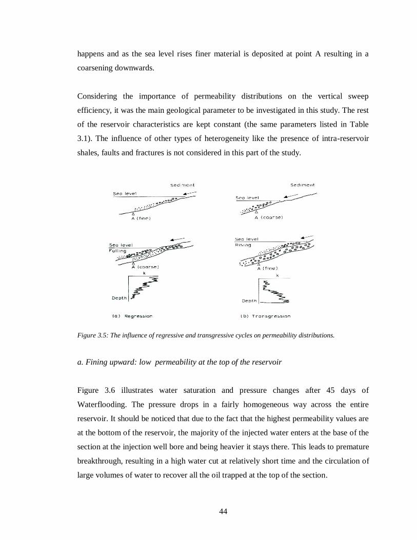
44

happens and as the sea level rises finer material is deposited at point A resulting in a

coarsening downwards.

Considering the importance of permeability distributions on the vertical sweep

efficiency, it was the main geological parameter to be investigated in this study. The rest

of the reservoir characteristics are kept constant (the same parameters listed in Table

3.1). The influence of other types of heterogeneity like the presence of intra-reservoir

shales, faults and fractures is not considered in this part of the study.

Figure 3.5: The influence of regressive and transgressive cycles on permeability distributions.

a. Fining upward: low permeability at the top of the reservoir

Figure 3.6 illustrates water saturation and pressure changes after 45 days of

Waterflooding. The pressure drops in a fairly homogeneous way across the entire

reservoir. It should be noticed that due to the fact that the highest permeability values are

at the bottom of the reservoir, the majority of the injected water enters at the base of the

section at the injection well bore and being heavier it stays there. This leads to premature

breakthrough, resulting in a high water cut at relatively short time and the circulation of

large volumes of water to recover all the oil trapped at the top of the section.

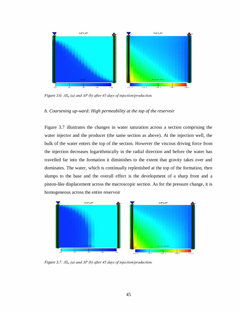
45


b. Coarsening up-ward: High permeability at the top of the reservoir

Figure 3.7 illustrates the changes in water saturation across a section comprising the

water injector and the producer (the same section as above). At the injection well, the

bulk of the water enters the top of the section. However the viscous driving force from

the injection decreases logarithmically in the radial direction and before the water has

travelled far into the formation it diminishes to the extent that gravity takes over and

dominates. The water, which is continually replenished at the top of the formation, then

slumps to the base and the overall effect is the development of a sharp front and a

piston-like displacement across the macroscopic section. As for the pressure change, it is

homogeneous across the entire reservoir


46

3.3 Petrophysical modelling

It is necessary for any time-lapse seismic analysis to have an understanding of the

changes in P-wave (compressional) velocity, S-wave (shear) velocity, and density as

fluid or rock properties change, in order to recognize or predict the effect of changes in

seismic amplitudes and travel-times. The petro-elastic modelling links these two

domains: the reservoir domain (flow simulation) and the elastic domain (wave

propagation) (Falcone et al., 2004). This appendix explains the conventional petro-

elastic modelling used to convert the fluid properties (pressures, saturations, fluid

densities) and rock properties (porosities, clay content, rock frame bulk moduli) into the

saturated elastic moduli, and hence determines P-wave velocities, S-wave velocities and

densities.

The static (e.g. porosity, net-to-gross, permeability) and dynamic grid properties (e.g.

pressure and saturation output from the simulator) are the inputs to a rock and fluid

physics calculation that computes the P- and S-wave velocity and density grids of the

same size as the simulation grids for each of the chosen production times. The results of

this petro-elastic transformation could be sufficient for feasibility 4D seismic tests, or for

part of a more sophisticated full-scale simulator to seismic workflow. For reservoirs

without compaction issues due to geomechanical effects, the petro-elastic model consists

of three main categories: fluid substitution, fluid-related pressure effects, and the stress-

dependency of the rock frame. The properties of the reservoir fluid are determined using

the equations of Batzle and Wang (1992) described in Appendix B.

The petro-elastic transformation assumes an isotropic, linear elastic medium. Under

these assumptions, the elastic tensor will depend on two constants, the bulk modulus K

and the shear modulus μ. P-wave and S-wave velocities (Vp and VS respectively) can be

expressed as a function of these two elastic constants:

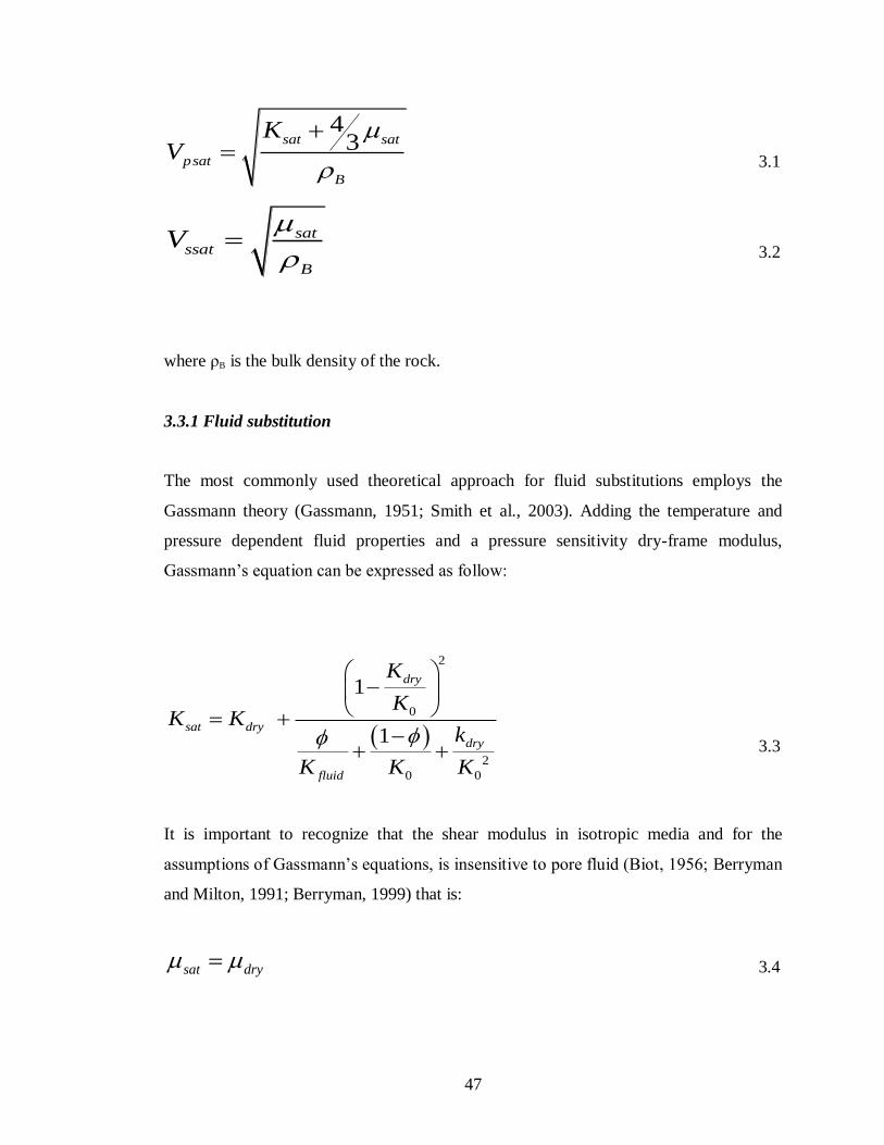
47

43sat sat

psat

B

KV

3.1

satssat

B

V

3.2

where ρB is the bulk density of the rock.

3.3.1 Fluid substitution

The most commonly used theoretical approach for fluid substitutions employs the

Gassmann theory (Gassmann, 1951; Smith et al., 2003). Adding the temperature and

pressure dependent fluid properties and a pressure sensitivity dry-frame modulus,

Gassmann’s equation can be expressed as follow:

2

0

2

0 0

1

1

dry

sat dry

dry

fluid

K

KK K

k

K K K

3.3

It is important to recognize that the shear modulus in isotropic media and for the

assumptions of Gassmann’s equations, is insensitive to pore fluid (Biot, 1956; Berryman

and Milton, 1991; Berryman, 1999) that is:

sat dry 3.4

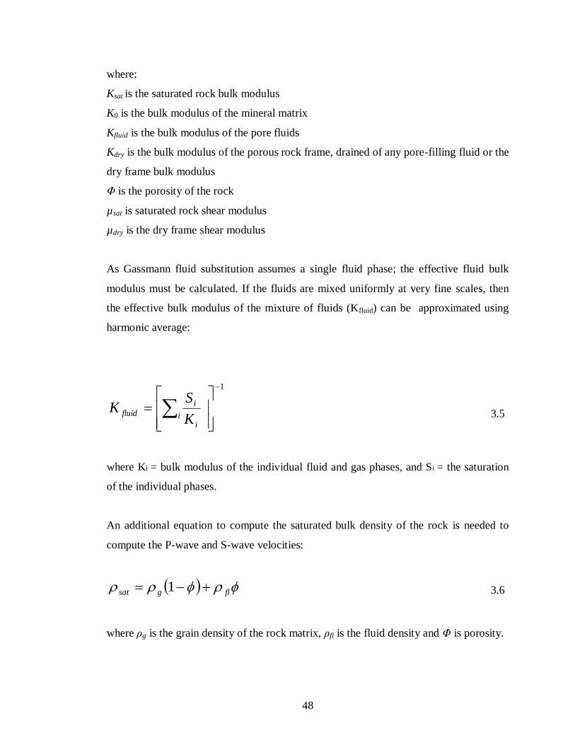
48

where:

Ksat is the saturated rock bulk modulus

K0 is the bulk modulus of the mineral matrix

Kfluid is the bulk modulus of the pore fluids

Kdry is the bulk modulus of the porous rock frame, drained of any pore-filling fluid or the

dry frame bulk modulus

Φ is the porosity of the rock

µsat is saturated rock shear modulus

µdry is the dry frame shear modulus

As Gassmann fluid substitution assumes a single fluid phase; the effective fluid bulk

modulus must be calculated. If the fluids are mixed uniformly at very fine scales, then

the effective bulk modulus of the mixture of fluids (Kfluid) can be approximated using

harmonic average:

1

i

i

i

fluidK

SK 3.5

where Ki = bulk modulus of the individual fluid and gas phases, and Si = the saturation

of the individual phases.

An additional equation to compute the saturated bulk density of the rock is needed to

compute the P-wave and S-wave velocities:

flgsat 1 3.6

where ρg is the grain density of the rock matrix, ρfl is the fluid density and Φ is porosity.

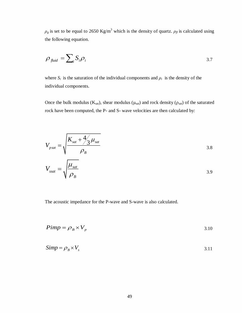
49

ρg is set to be equal to 2650 Kg/m3 which is the density of quartz. ρfl is calculated using

the following equation.

i iifluid S 3.7

where Si is the saturation of the individual components and ρi is the density of the

individual components.

Once the bulk modulus (Ksat), shear modulus (μsat) and rock density (ρsat) of the saturated

rock have been computed, the P- and S- wave velocities are then calculated by:

43sat sat

psat

B

KV

3.8

satssat

B

V

3.9

The acoustic impedance for the P-wave and S-wave is also calculated.

B pPimp V 3.10

B sSimp V 3.11

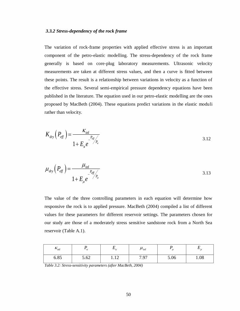
50

3.3.2 Stress-dependency of the rock frame

The variation of rock-frame properties with applied effective stress is an important

component of the petro-elastic modelling. The stress-dependency of the rock frame

generally is based on core-plug laboratory measurements. Ultrasonic velocity

measurements are taken at different stress values, and then a curve is fitted between

these points. The result is a relationship between variations in velocity as a function of

the effective stress. Several semi-empirical pressure dependency equations have been

published in the literature. The equation used in our petro-elastic modelling are the ones

proposed by MacBeth (2004). These equations predict variations in the elastic moduli

rather than velocity.

inf

1eff

dry eff P

P

K P

E e

3.12

inf

1eff

dry eff P

P

P

E e

3.13

The value of the three controlling parameters in each equation will determine how

responsive the rock is to applied pressure. MacBeth (2004) compiled a list of different

values for these parameters for different reservoir settings. The parameters chosen for

our study are those of a moderately stress sensitive sandstone rock from a North Sea

reservoir (Table A.1).

inf P E inf P E

6.85 5.62 1.12 7.97 5.06 1.08

Table 3.2: Stress-sensitivity parameters (after MacBeth, 2004)

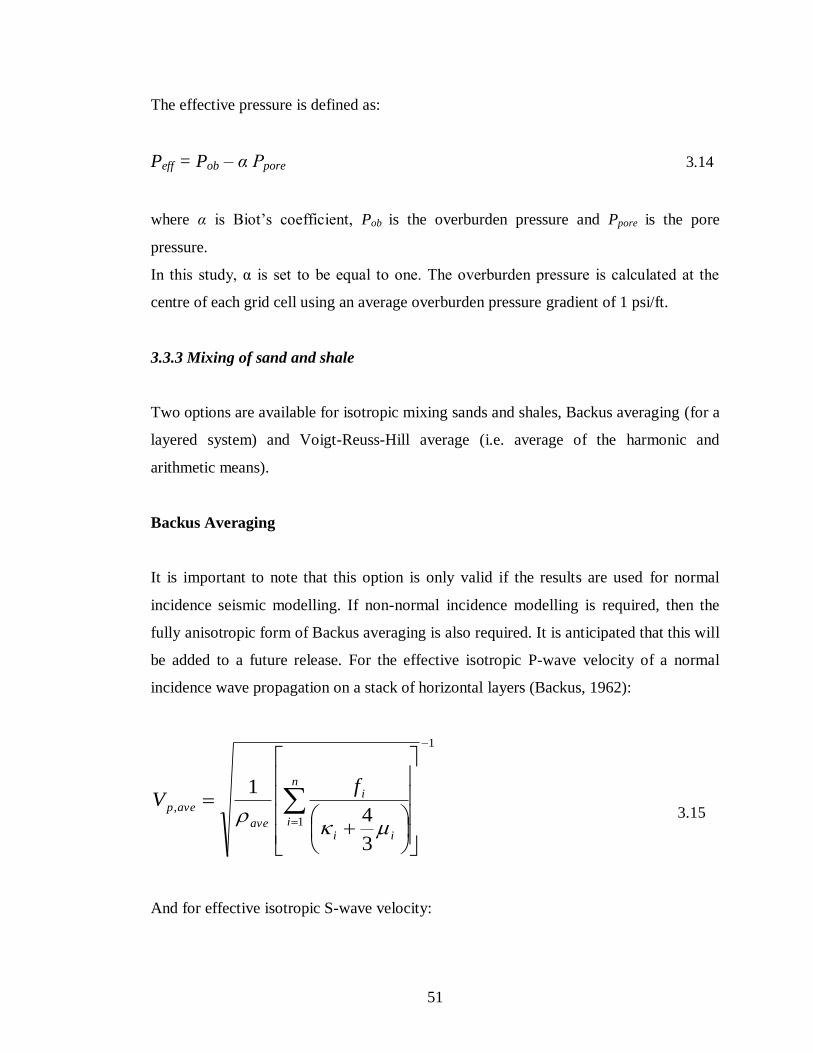
51

The effective pressure is defined as:

Peff = Pob – α Ppore 3.14

where α is Biot’s coefficient, Pob is the overburden pressure and Ppore is the pore

pressure.

In this study, α is set to be equal to one. The overburden pressure is calculated at the

centre of each grid cell using an average overburden pressure gradient of 1 psi/ft.

3.3.3 Mixing of sand and shale

Two options are available for isotropic mixing sands and shales, Backus averaging (for a

layered system) and Voigt-Reuss-Hill average (i.e. average of the harmonic and

arithmetic means).

Backus Averaging

It is important to note that this option is only valid if the results are used for normal

incidence seismic modelling. If non-normal incidence modelling is required, then the

fully anisotropic form of Backus averaging is also required. It is anticipated that this will

be added to a future release. For the effective isotropic P-wave velocity of a normal

incidence wave propagation on a stack of horizontal layers (Backus, 1962):

1

1

,

3

4

1

n

i

ii

i

ave

avep

fV

3.15

And for effective isotropic S-wave velocity:

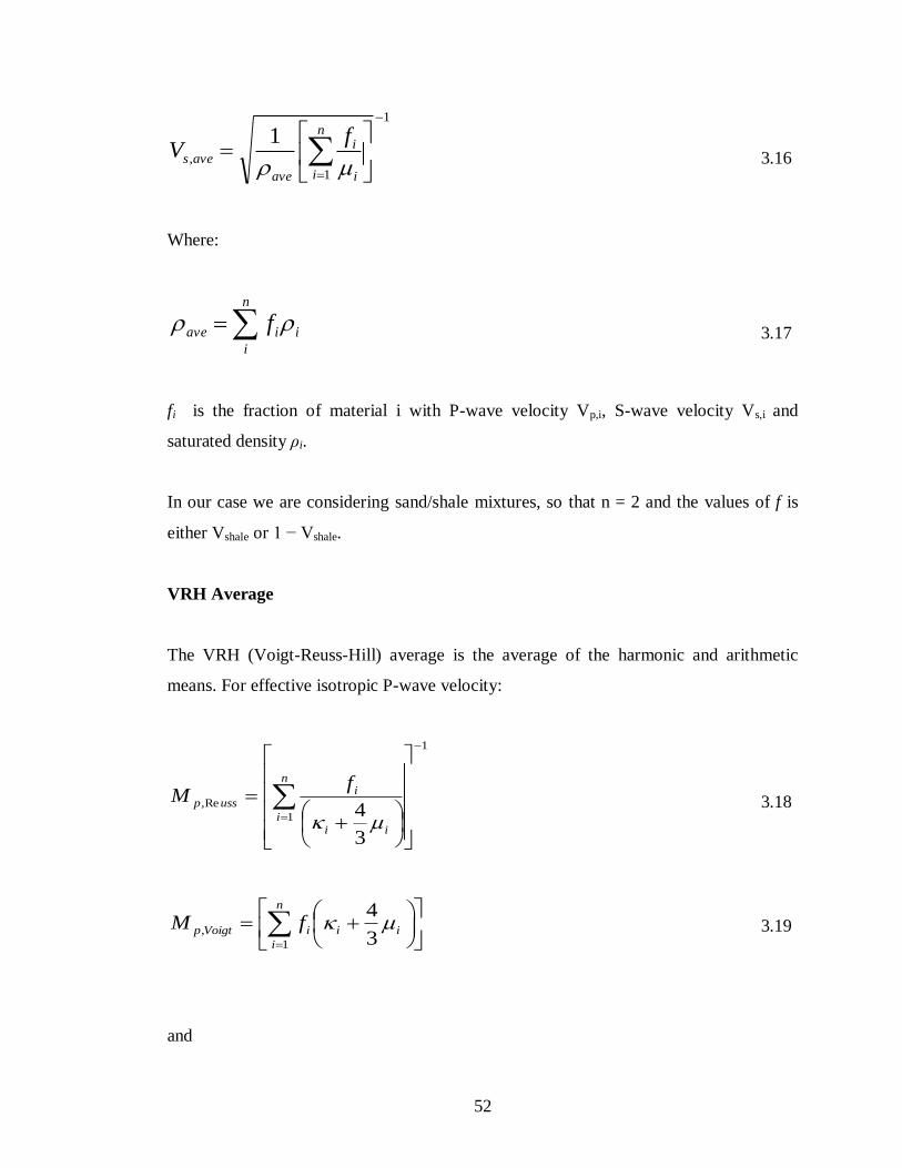
52

1

1

,

1

n

i i

i

ave

aves

fV

3.16

Where:

n

i

iiave f 3.17

fi is the fraction of material i with P-wave velocity Vp,i, S-wave velocity Vs,i and

saturated density ρi.

In our case we are considering sand/shale mixtures, so that n = 2 and the values of f is

either Vshale or 1 − Vshale.

VRH Average

The VRH (Voigt-Reuss-Hill) average is the average of the harmonic and arithmetic

means. For effective isotropic P-wave velocity:

1

1

Re,

3

4

n

iii

iussp

fM

3.18

n

i

iiiVoigtp fM1

,3

4 3.19

and

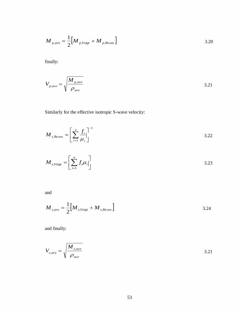
53

usspVoigtpavep MMM Re,,,2

1 3.20

finally:

ave

avep

avep

MV

,

, 3.21

Similarly for the effective isotropic S-wave velocity:

1

1

Re,

n

i i

iusss

fM

3.22

n

i

iiVoigts fM1

, 3.23

and

usssVoigtsaves MMM Re,,,2

1 3.24

and finally:

ave

aves

aves

MV

,

, 3.21

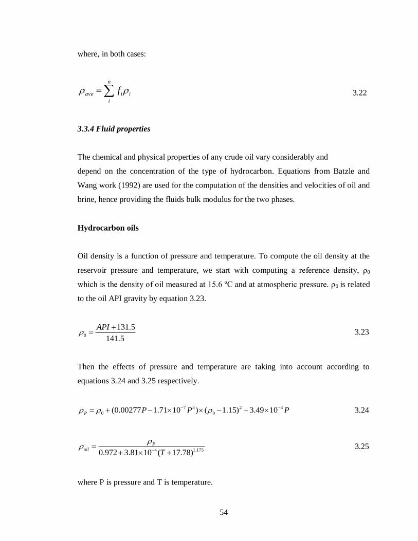
54

where, in both cases:

n

i

iiave f 3.22

3.3.4 Fluid properties

The chemical and physical properties of any crude oil vary considerably and

depend on the concentration of the type of hydrocarbon. Equations from Batzle and

Wang work (1992) are used for the computation of the densities and velocities of oil and

brine, hence providing the fluids bulk modulus for the two phases.

Hydrocarbon oils

Oil density is a function of pressure and temperature. To compute the oil density at the

reservoir pressure and temperature, we start with computing a reference density, ρ0

which is the density of oil measured at 15.6 ºC and at atmospheric pressure. ρ0 is related

to the oil API gravity by equation 3.23.

0

131.5

141.5

API

3.23

Then the effects of pressure and temperature are taking into account according to

equations 3.24 and 3.25 respectively.

7 3 2 4

0 0(0.00277 1.71 10 ) ( 1.15) 3.49 10P P P P 3.24

4 1.1750.972 3.81 10 ( 17.78)

Poil

T

3.25

where P is pressure and T is temperature.

55

The velocity of oil is a function the oil gravity, pressure and temperature. Equation 3.26

is used to obtain the oil velocity at the reservoir pressure and temperature.

1 12 215450(77.1 ) 3.7 4.64 0.0115(0.36 1)oilV API T P API TP

3.26

where P is pressure, T is temperature and API is the oil gravity.

The bulk modulus of oil is then calculated using equation 3.27

2

oil oil oilK V 3.27

Brine

Batzle and Wang equations are used to compute the bulk modulus of the brine. The

density of pure water is first computed using equations 3.28, and then the density of

brine is computed using equation 3.29.

6 2 3 2

5 3 2 2

1 1 10 ( 80 3.3 0.00175 489 2 0.016

1.3 10 0.333 0.002 )

water T T T P TP T P

T P P TP

3.28

6{0.668 0.44 1 10

300 2400 80 3 3300 13 47 }

brine water S S

P PS T T S P PS

3.29

where T is temperature, P is pressure and S is the brine salinity

The velocity of pure water is computed using equation 3.30.

4 3

0 0

i j

water ij

i j

V w T P

3.30

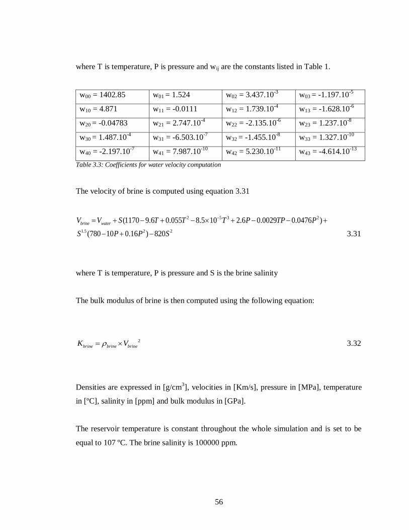
56

where T is temperature, P is pressure and wij are the constants listed in Table 1.

w00 = 1402.85 w01 = 1.524 w02 = 3.437.10-3

w03 = -1.197.10-5

w10 = 4.871 w11 = -0.0111 w12 = 1.739.10-4

w13 = -1.628.10-6

w20 = -0.04783 w21 = 2.747.10-4

w22 = -2.135.10-6

w23 = 1.237.10-8

w30 = 1.487.10-4

w31 = -6.503.10-7

w32 = -1.455.10-8

w33 = 1.327.10-10

w40 = -2.197.10-7

w41 = 7.987.10-10

w42 = 5.230.10-11

w43 = -4.614.10-13

Table 3.3: Coefficients for water velocity computation

The velocity of brine is computed using equation 3.31

2 5 3 2

1.5 2 2

(1170 9.6 0.055 8.5 10 2.6 0.0029 0.0476 )

(780 10 0.16 ) 820

brine waterV V S T T T P TP P

S P P S

3.31

where T is temperature, P is pressure and S is the brine salinity

The bulk modulus of brine is then computed using the following equation:

2

brine brine brineK V 3.32

Densities are expressed in [g/cm3], velocities in [Km/s], pressure in [MPa], temperature

in [ºC], salinity in [ppm] and bulk modulus in [GPa].

The reservoir temperature is constant throughout the whole simulation and is set to be

equal to 107 ºC. The brine salinity is 100000 ppm.

57

3.3.5 Homogeneous reservoir: injection with pressure support

The petro-elastic transform gives cubes of P-wave velocities (Vp), S-wave velocities

(Vs), and densities (Rho) at each grid cell. P-wave impedance (Pimp) and S-wave

impedance (Simp) are then computed. Vp, Vs and Rho grids have the same dimensions

as the 3D simulation grid. In this section, we will display the results at a cross-section

through the middle of the reservoir, where the water injector and the producer are placed

during the simulation (Crossline 10).

The changes in the rock physical properties are the highest in the water-invaded areas.

We obtained very low changes in Vp, Vs, Pimp and Simp in the area ahead of the

waterfront, where only pressure changes affect the petro-elastic properties.

Vp and Vs respond to Waterflooding in two contrasting ways. Vp decreased by a

maximum of -0.073 m/s (-0.0024%) around the oil producer ahead of the waterfront and

the maximum increase was 131.529 m/s (4.273%) around the water injector behind the

waterfront. Vs decreased by a maximum of -25.0431 m/s (-1.291%) behind the

waterfront and the maximum increase is 0.56 m/s (0.0289%) ahead of the waterfront. P-

impedance relative changes vary between -0.0047% and 7.0623%, while the changes in

S-impedance are between 0.0215% and 1.35% (Figure 3.8).

The pressure being maintained constant, the observed changes can be directly linked to

saturation changes. The waterfront forms a transition zone between the water-saturated

and oil saturated parts of the reservoir. To ascertain the extent of this transition zone, a

row of cells at the mid-depth of the reservoir (layer 30) was extracted from the P-

impedance 10th cross-line (Figure 3.9). For saturation changes equal to or greater than

60% (inline 10 and behind) the impedance change is varying between 7% for a Sw of

90% and 5.5% for a Sw of 60%. The impedance values decrease exponentially in the

transition zone between inline 10 and 14, falling to almost 0% where no saturation

changes occurred. This transition zone, which forms the waterfront of the interface

between the displacing fluid, water, and the displaced fluid, oil, extends over 20 feet. In

the next section we will examine the seismic detectability of this zone.

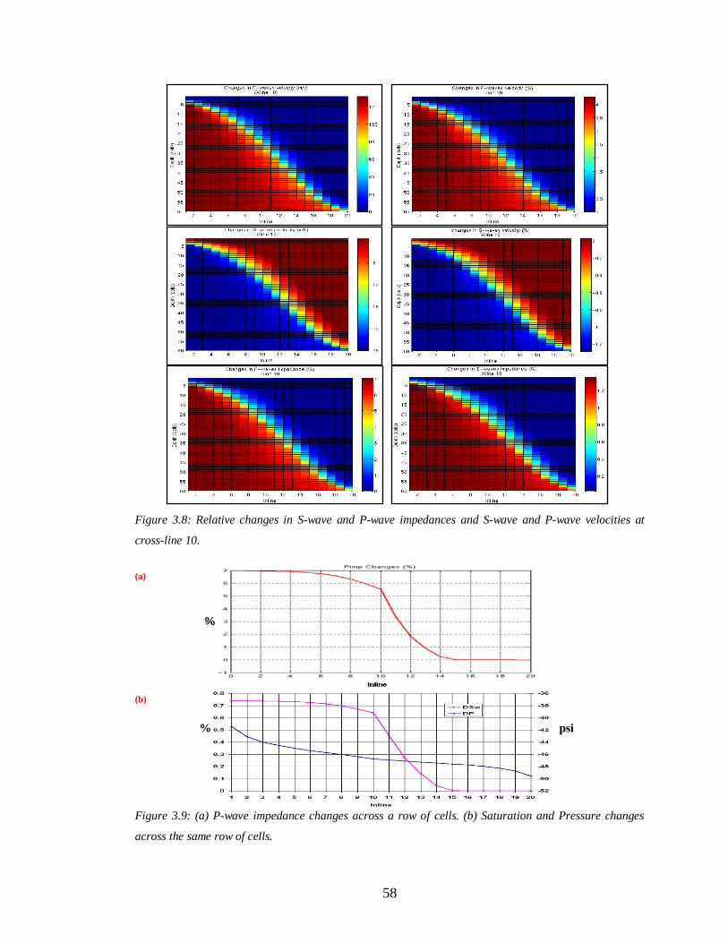
58

Figure 3.8: Relative changes in S-wave and P-wave impedances and S-wave and P-wave velocities at

cross-line 10.

(a)

%

(b) % psi

Figure 3.9: (a) P-wave impedance changes across a row of cells. (b) Saturation and Pressure changes

across the same row of cells.

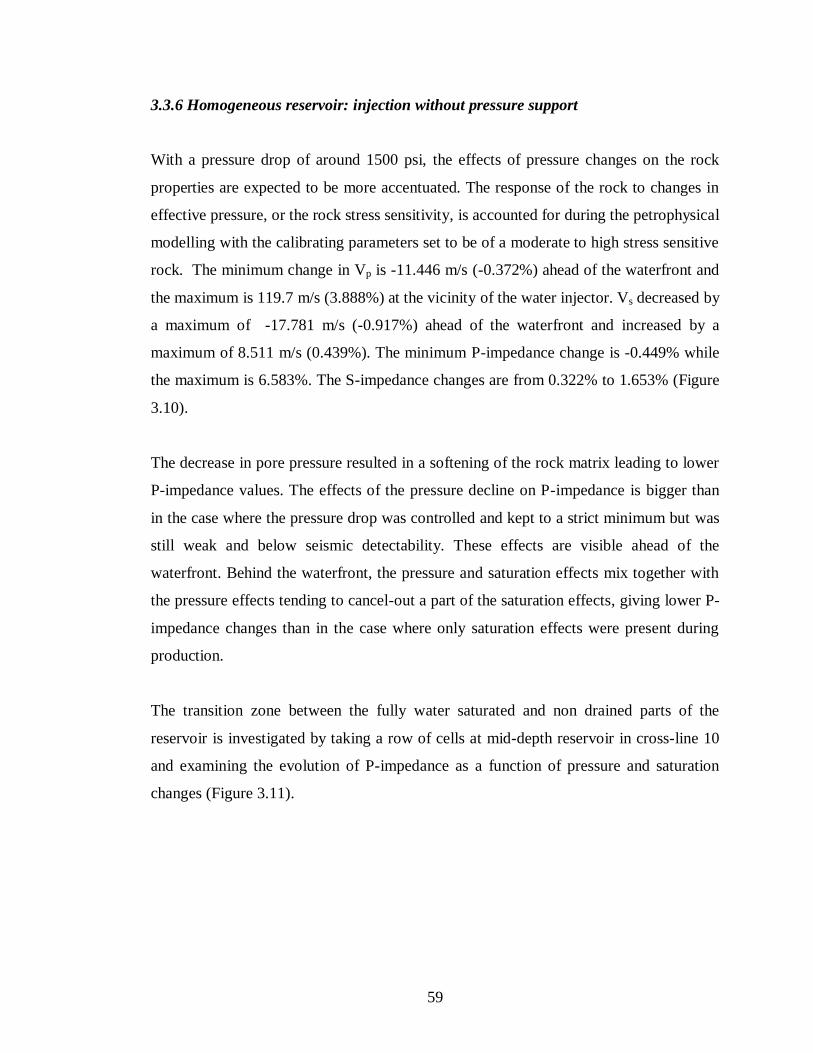
59

3.3.6 Homogeneous reservoir: injection without pressure support

With a pressure drop of around 1500 psi, the effects of pressure changes on the rock

properties are expected to be more accentuated. The response of the rock to changes in

effective pressure, or the rock stress sensitivity, is accounted for during the petrophysical

modelling with the calibrating parameters set to be of a moderate to high stress sensitive

rock. The minimum change in Vp is -11.446 m/s (-0.372%) ahead of the waterfront and

the maximum is 119.7 m/s (3.888%) at the vicinity of the water injector. Vs decreased by

a maximum of -17.781 m/s (-0.917%) ahead of the waterfront and increased by a

maximum of 8.511 m/s (0.439%). The minimum P-impedance change is -0.449% while

the maximum is 6.583%. The S-impedance changes are from 0.322% to 1.653% (Figure

3.10).

The decrease in pore pressure resulted in a softening of the rock matrix leading to lower

P-impedance values. The effects of the pressure decline on P-impedance is bigger than

in the case where the pressure drop was controlled and kept to a strict minimum but was

still weak and below seismic detectability. These effects are visible ahead of the

waterfront. Behind the waterfront, the pressure and saturation effects mix together with

the pressure effects tending to cancel-out a part of the saturation effects, giving lower P-

impedance changes than in the case where only saturation effects were present during

production.

The transition zone between the fully water saturated and non drained parts of the

reservoir is investigated by taking a row of cells at mid-depth reservoir in cross-line 10

and examining the evolution of P-impedance as a function of pressure and saturation

changes (Figure 3.11).

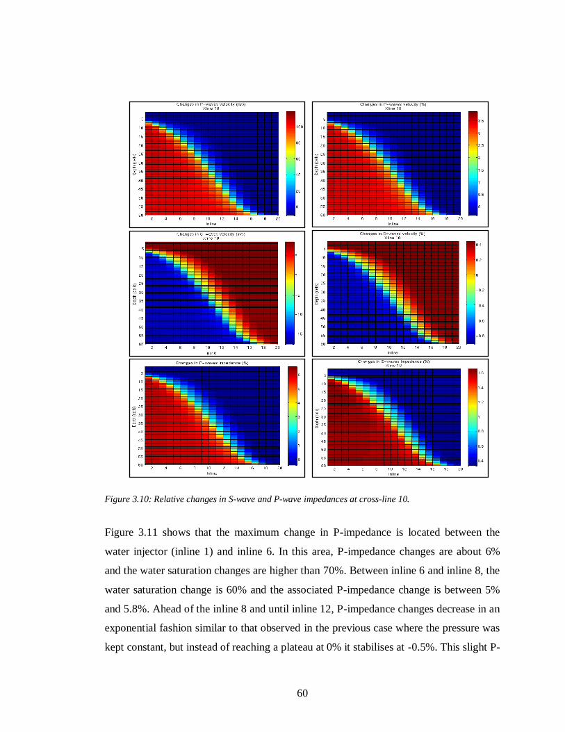
60

Figure 3.10: Relative changes in S-wave and P-wave impedances at cross-line 10.

Figure 3.11 shows that the maximum change in P-impedance is located between the

water injector (inline 1) and inline 6. In this area, P-impedance changes are about 6%

and the water saturation changes are higher than 70%. Between inline 6 and inline 8, the

water saturation change is 60% and the associated P-impedance change is between 5%

and 5.8%. Ahead of the inline 8 and until inline 12, P-impedance changes decrease in an

exponential fashion similar to that observed in the previous case where the pressure was

kept constant, but instead of reaching a plateau at 0% it stabilises at -0.5%. This slight P-

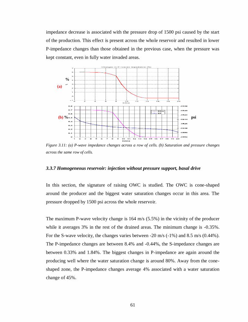
61

impedance decrease is associated with the pressure drop of 1500 psi caused by the start

of the production. This effect is present across the whole reservoir and resulted in lower

P-impedance changes than those obtained in the previous case, when the pressure was

kept constant, even in fully water invaded areas.

%

(a)

(b) % psi

Figure 3.11: (a) P-wave impedance changes across a row of cells. (b) Saturation and pressure changes

across the same row of cells.

3.3.7 Homogeneous reservoir: injection without pressure support, basal drive

In this section, the signature of raising OWC is studied. The OWC is cone-shaped

around the producer and the biggest water saturation changes occur in this area. The

pressure dropped by 1500 psi across the whole reservoir.

The maximum P-wave velocity change is 164 m/s (5.5%) in the vicinity of the producer

while it averages 3% in the rest of the drained areas. The minimum change is -0.35%.

For the S-wave velocity, the changes varies between -20 m/s (-1%) and 8.5 m/s (0.44%).

The P-impedance changes are between 8.4% and -0.44%, the S-impedance changes are

between 0.33% and 1.84%. The biggest changes in P-impedance are again around the

producing well where the water saturation change is around 80%. Away from the cone-

shaped zone, the P-impedance changes average 4% associated with a water saturation

change of 45%.

62

Even though the pressure decline is exactly the same as for the previous example with

edge drive, we obtained higher P-impedance changes in the water invaded area for

similar water saturation changes.

(a)

%

(b) % psi

Figure 3.12: (a) P-wave impedance changes across a row of cells at the producer location. (b) Saturation

and pressure changes across the same row of cells.

A column of cells was extracted at the producer location and the impedance changes are

plotted in Figure 3.12 (a). Figure 3.12 (b) shows the saturation changes across those

cells. The acoustic impedance profiles are closely related to the water saturation changes

3.3.8 Heterogeneous reservoir: fining upward

For this study, the average reservoir pressure dropped by 1500 psi. The combined effects

of saturation and pressure changes are illustrated. The P-wave velocity changes vary

from -11.4 m/s (-0.37%) to 122.2 m/s (3.96%). The S-wave velocity changes are from -

18 m/s (-0.92%) to 3.96 m/s (0.44%). The maximum decrease of P-wave impedance is -

0.45% around the producer. The maximum increase is 6.7% at the vicinity of the water

injector. For the S-wave impedance, the changes vary from 0.32% to 1.66% (Figure

3.13).

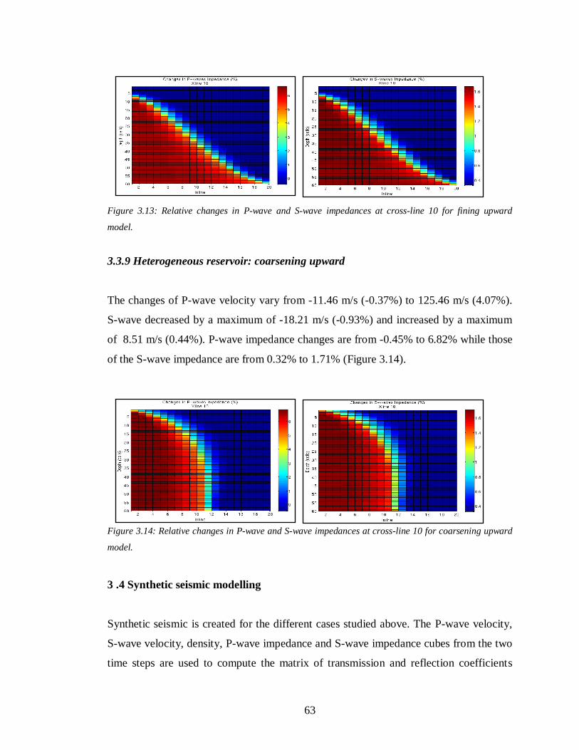
63

Figure 3.13: Relative changes in P-wave and S-wave impedances at cross-line 10 for fining upward

model.

3.3.9 Heterogeneous reservoir: coarsening upward

The changes of P-wave velocity vary from -11.46 m/s (-0.37%) to 125.46 m/s (4.07%).

S-wave decreased by a maximum of -18.21 m/s (-0.93%) and increased by a maximum

of 8.51 m/s (0.44%). P-wave impedance changes are from -0.45% to 6.82% while those

of the S-wave impedance are from 0.32% to 1.71% (Figure 3.14).

Figure 3.14: Relative changes in P-wave and S-wave impedances at cross-line 10 for coarsening upward

model.

3 .4 Synthetic seismic modelling

Synthetic seismic is created for the different cases studied above. The P-wave velocity,

S-wave velocity, density, P-wave impedance and S-wave impedance cubes from the two

time steps are used to compute the matrix of transmission and reflection coefficients

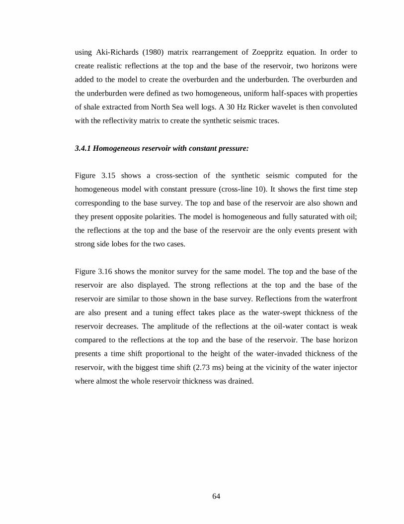
64

using Aki-Richards (1980) matrix rearrangement of Zoeppritz equation. In order to

create realistic reflections at the top and the base of the reservoir, two horizons were

added to the model to create the overburden and the underburden. The overburden and

the underburden were defined as two homogeneous, uniform half-spaces with properties

of shale extracted from North Sea well logs. A 30 Hz Ricker wavelet is then convoluted

with the reflectivity matrix to create the synthetic seismic traces.

3.4.1 Homogeneous reservoir with constant pressure:

Figure 3.15 shows a cross-section of the synthetic seismic computed for the

homogeneous model with constant pressure (cross-line 10). It shows the first time step

corresponding to the base survey. The top and base of the reservoir are also shown and

they present opposite polarities. The model is homogeneous and fully saturated with oil;

the reflections at the top and the base of the reservoir are the only events present with

strong side lobes for the two cases.

Figure 3.16 shows the monitor survey for the same model. The top and the base of the

reservoir are also displayed. The strong reflections at the top and the base of the

reservoir are similar to those shown in the base survey. Reflections from the waterfront

are also present and a tuning effect takes place as the water-swept thickness of the

reservoir decreases. The amplitude of the reflections at the oil-water contact is weak

compared to the reflections at the top and the base of the reservoir. The base horizon

presents a time shift proportional to the height of the water-invaded thickness of the

reservoir, with the biggest time shift (2.73 ms) being at the vicinity of the water injector

where almost the whole reservoir thickness was drained.

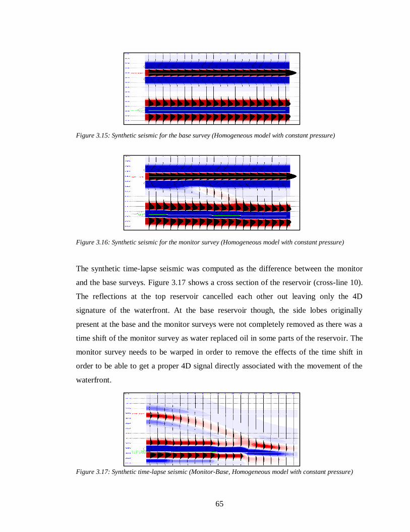
65

Figure 3.15: Synthetic seismic for the base survey (Homogeneous model with constant pressure)

Figure 3.16: Synthetic seismic for the monitor survey (Homogeneous model with constant pressure)

The synthetic time-lapse seismic was computed as the difference between the monitor

and the base surveys. Figure 3.17 shows a cross section of the reservoir (cross-line 10).

The reflections at the top reservoir cancelled each other out leaving only the 4D

signature of the waterfront. At the base reservoir though, the side lobes originally

present at the base and the monitor surveys were not completely removed as there was a

time shift of the monitor survey as water replaced oil in some parts of the reservoir. The

monitor survey needs to be warped in order to remove the effects of the time shift in

order to be able to get a proper 4D signal directly associated with the movement of the

waterfront.

Figure 3.17: Synthetic time-lapse seismic (Monitor-Base, Homogeneous model with constant pressure)

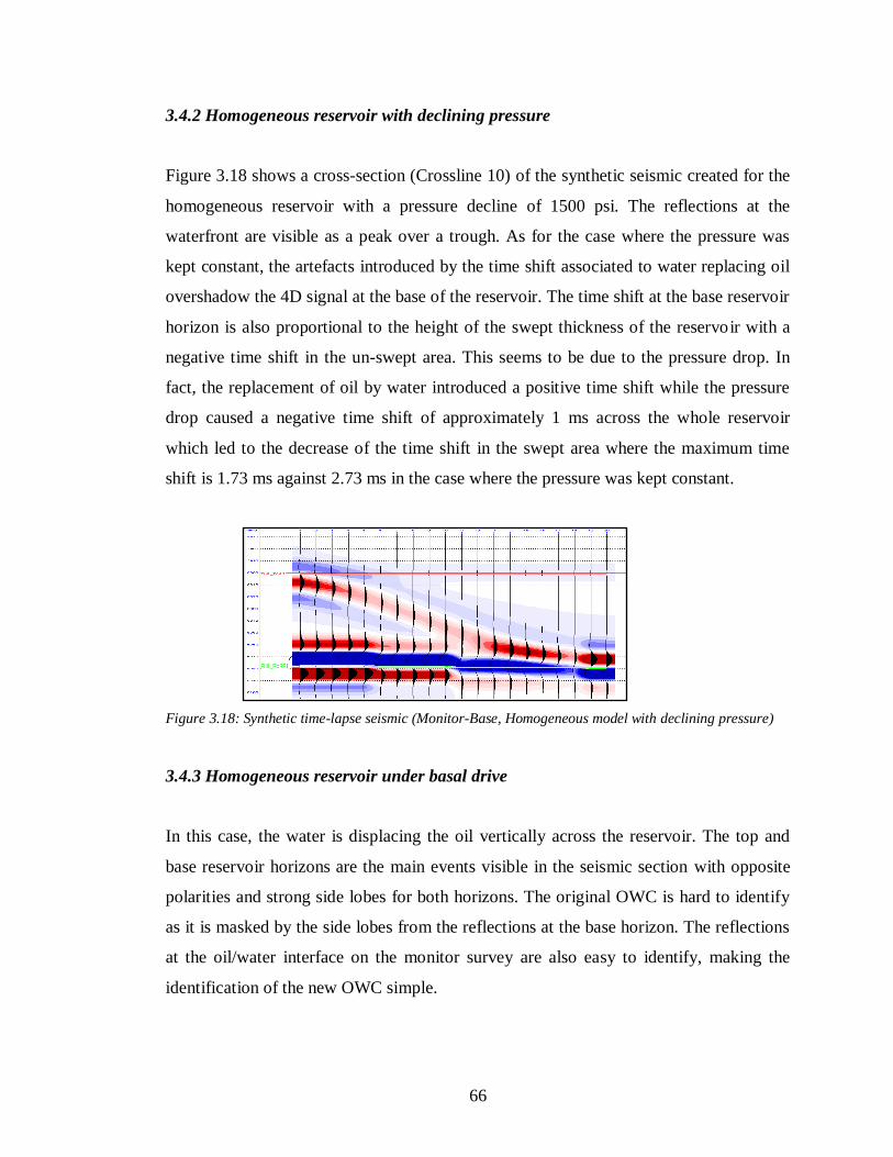
66

3.4.2 Homogeneous reservoir with declining pressure

Figure 3.18 shows a cross-section (Crossline 10) of the synthetic seismic created for the

homogeneous reservoir with a pressure decline of 1500 psi. The reflections at the

waterfront are visible as a peak over a trough. As for the case where the pressure was

kept constant, the artefacts introduced by the time shift associated to water replacing oil

overshadow the 4D signal at the base of the reservoir. The time shift at the base reservoir

horizon is also proportional to the height of the swept thickness of the reservoir with a

negative time shift in the un-swept area. This seems to be due to the pressure drop. In

fact, the replacement of oil by water introduced a positive time shift while the pressure

drop caused a negative time shift of approximately 1 ms across the whole reservoir

which led to the decrease of the time shift in the swept area where the maximum time

shift is 1.73 ms against 2.73 ms in the case where the pressure was kept constant.

Figure 3.18: Synthetic time-lapse seismic (Monitor-Base, Homogeneous model with declining pressure)

3.4.3 Homogeneous reservoir under basal drive

In this case, the water is displacing the oil vertically across the reservoir. The top and

base reservoir horizons are the main events visible in the seismic section with opposite

polarities and strong side lobes for both horizons. The original OWC is hard to identify

as it is masked by the side lobes from the reflections at the base horizon. The reflections

at the oil/water interface on the monitor survey are also easy to identify, making the

identification of the new OWC simple.

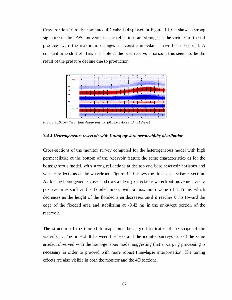
67

Cross-section 10 of the computed 4D cube is displayed in Figure 3.19. It shows a strong

signature of the OWC movement. The reflections are stronger at the vicinity of the oil

producer were the maximum changes in acoustic impedance have been recorded. A

constant time shift of -1ms is visible at the base reservoir horizon; this seems to be the

result of the pressure decline due to production.

Figure 3.19: Synthetic time-lapse seismic (Monitor-Base, Basal drive)

3.4.4 Heterogeneous reservoir with fining upward permeability distribution

Cross-sections of the monitor survey computed for the heterogeneous model with high

permeabilities at the bottom of the reservoir feature the same characteristics as for the

homogeneous model, with strong reflections at the top and base reservoir horizons and

weaker reflections at the waterfront. Figure 3.20 shows the time-lapse seismic section.

As for the homogeneous case, it shows a clearly detectable waterfront movement and a

positive time shift at the flooded areas, with a maximum value of 1.35 ms which

decreases as the height of the flooded area decreases until it reaches 0 ms toward the

edge of the flooded area and stabilizing at -0.42 ms in the un-swept portion of the

reservoir.

The structure of the time shift map could be a good indicator of the shape of the

waterfront. The time shift between the base and the monitor surveys caused the same

artefact observed with the homogeneous model suggesting that a warping processing is

necessary in order to proceed with more robust time-lapse interpretation. The tuning

effects are also visible in both the monitor and the 4D sections.

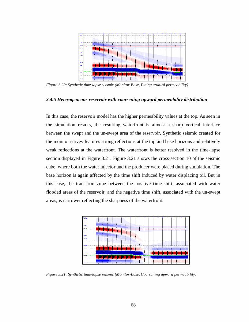
68

Figure 3.20: Synthetic time-lapse seismic (Monitor-Base, Fining upward permeability)

3.4.5 Heterogeneous reservoir with coarsening upward permeability distribution

In this case, the reservoir model has the higher permeability values at the top. As seen in

the simulation results, the resulting waterfront is almost a sharp vertical interface

between the swept and the un-swept area of the reservoir. Synthetic seismic created for

the monitor survey features strong reflections at the top and base horizons and relatively

weak reflections at the waterfront. The waterfront is better resolved in the time-lapse

section displayed in Figure 3.21. Figure 3.21 shows the cross-section 10 of the seismic

cube, where both the water injector and the producer were placed during simulation. The

base horizon is again affected by the time shift induced by water displacing oil. But in

this case, the transition zone between the positive time-shift, associated with water

flooded areas of the reservoir, and the negative time shift, associated with the un-swept

areas, is narrower reflecting the sharpness of the waterfront.

Figure 3.21: Synthetic time-lapse seismic (Monitor-Base, Coarsening upward permeability)

69

3.5 Comparative study

In this section, a comparative study is carried out to examine the petrophysical

modelling results for the different scenarios studied. The effects of those differences on

the corresponding time-lapse signature are highlighted.

Table 3.2 shows a summary of the changes in percentage for the different reservoir rock

properties after Waterflooding for each scenario.

The maximum changes in P-wave impedance are of similar magnitude for the different

Waterflooding scenarios. The petrophysical modelling does not give any indication of

the stability of the waterfront.

The pressure change during Waterflooding has an opposite effect on rock properties to

that of saturation changes. In the four scenarios run with reservoir pressure declining by

up to 1500 psi, we had similar minimum and maximum changes in P-wave impedance

values. The minimum P-wave impedance change is around -0.5% regardless of the

geology of the reservoir. This minimum change happened ahead of the waterfront,

where no saturation changes had yet occurred . When the pressure was kept constant

during simulation this change was almost zero (-0.004%).

While saturation changes during Waterflooding increase the P-impedance in case of

drainage (oil swept by water), pressure change has a global dimming effect on the P-

wave impedances. It happens very briefly after the start of the simulation and spreads

across the whole reservoir.

The petroelsatic changes in the reservoir rock properties are the strongest behind the

waterfront. The waterfront represents a transition area spread over a couple of feet where

the magnitude of the changes decreases gradually.

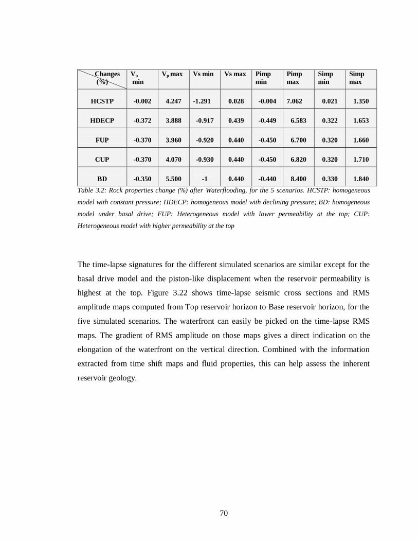
70

Table 3.2: Rock properties change (%) after Waterflooding, for the 5 scenarios. HCSTP: homogeneous

model with constant pressure; HDECP: homogeneous model with declining pressure; BD: homogeneous

model under basal drive; FUP: Heterogeneous model with lower permeability at the top; CUP:

Heterogeneous model with higher permeability at the top

The time-lapse signatures for the different simulated scenarios are similar except for the

basal drive model and the piston-like displacement when the reservoir permeability is

highest at the top. Figure 3.22 shows time-lapse seismic cross sections and RMS

amplitude maps computed from Top reservoir horizon to Base reservoir horizon, for the

five simulated scenarios. The waterfront can easily be picked on the time-lapse RMS

maps. The gradient of RMS amplitude on those maps gives a direct indication on the

elongation of the waterfront on the vertical direction. Combined with the information

extracted from time shift maps and fluid properties, this can help assess the inherent

reservoir geology.

Changes

(%)

Model

Vp

min

Vp max Vs min Vs max Pimp

min

Pimp

max

Simp

min

Simp

max

HCSTP

-0.002

4.247

-1.291

0.028

-0.004

7.062

0.021

1.350

HDECP

-0.372

3.888

-0.917

0.439

-0.449

6.583

0.322

1.653

FUP

-0.370

3.960

-0.920

0.440

-0.450

6.700

0.320

1.660

CUP

-0.370

4.070

-0.930

0.440

-0.450

6.820

0.320

1.710

BD

-0.350

5.500

-1

0.440

-0.440

8.400

0.330

1.840

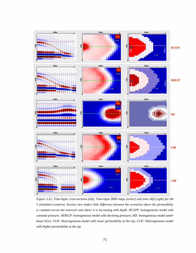
71

Figure 3.22: Time-lapse cross-sections (left), Time-lapse RMS maps (centre) and time shift (right) for the

5 simulated scenarios. Section view makes little difference between the scenarios where the permeability

is constant across the reservoir and where it is increasing with depth. HCSTP: homogeneous model with

constant pressure; HDECP: homogeneous model with declining pressure; BD: homogeneous model under

basal drive; FUP: Heterogeneous model with lower permeability at the top; CUP: Heterogeneous model

with higher permeability at the top

72

3.6 Conclusion

Waterflooding of a series of thick, idealised reservoir models, consisting of a thick block

of sand with varying geological complexity, was simulated. Several scenarios of

Waterflooding and their associated petrophysical and time-lapse signatures were studied.

Fluid flow simulation showed that the sweep efficiency is mainly controlled by the

reservoir geology, i.e. horizontal permeability, NTG, and vertical hydraulic

communication between the reservoir layers. Time-lapse seismic analysis showed that

inferring OWC on RMS maps is straightforward. The swept and un-swept areas exhibit

opposite polarities and the transition zone where both phases (oil and water) coexist is

easily interpretable. It is still challenging, though, to infer the vertical water distribution

inside the reservoir.

The time-lapse signature of Waterflooding is mainly controlled by fluid saturation

changes within the reservoir rocks. Waterflooding a reservoir while maintaining the pore

pressure constant produced the same waterfront profile as when the pressure was

allowed to drop significantly.

The petrophysical modelling showed that the substitution of oil by water within the

reservoir pores produced the same level of change in the petro-elastic properties,

regardless of the geology of the reservoir. In fact, changes in Vp, Vs and Rho were

comparable for all the Waterflooding cases where the pressure dropped. In the case

where pressure was kept constant, Vp, Vs and Rho changes were higher. The pressure

decline had a global dimming effect on the time-lapse seismic signature of

Waterflooding, due mainly to the absence of any reservoir compartmentalisation.

Seismic attributes analysis showed that in an idealised environment, and in the absence

of any 4D seismic noise, the waterfront is visible on both vertical cross-sections and

RMS maps. The combination of several seismic attributes may be needed for a more

accurate mapping of the fluids contacts especially in cases when Waterflooding

heterogeneous reservoirs. This simple reservoir model is meant to be representative of a

73

high net-to-gross flow unit inside a turbidite reservoir. The next step in our study will

focus on simulating a realistic turbidite reservoir and investigate the different time-lapse

signature in a geologically complex setting.

74

Chapter 4

Geological overview and challenges for turbidite systems

This chapter gives a geological description of deepwater turbidite reservoirs and their

different elements. The seismic characteristics of these different elements are

highlighted through example from real reservoirs. The challenges for an optimal deep

water turbidite reservoir management are also discussed. The AINSAII geological and

simulation models are presented. Waterflooding simulation results are discussed.

75

4.1 Introduction

With the increased importance of deepwater exploration and development activities

worldwide, a huge amount of work has been done to describe and understand turbidite

systems. Over the last 50 years, data on composition, texture and structures of

sedimentary rocks have grown enormously.The physical processes of sedimentation and

their importance in understanding sedimentary structures have been topic of growning

interest. This has come about as a response to the emphasis on the need to provide

detailed reservoir description of deepwater turbidite reservoirs.

The biggest challenge for hydrocarbon exploration and production is to produce the

reservoir with the maximum recovery factor. A reservoir description is a comprehensive

three-dimensional picture showing the distribution and continuity of the rocks, pores,

and fluids of the reservoir and aquifer system, including flow barriers. For prospect

evaluation and play development, it is crucial to obtain this information during the

exploration phase. The activity intensifies once a discovery is made. As a reservoir or

field goes through the typical life cycle of discovery, appraisal, planning, development

and reservoir monitoring, a more complete reservoir description is both necessary and

possible.

The principal geophysical, geological, and petro-physical contributions to reservoir

description are the external geometry of the reservoir; the internal geometry of the

reservoir, including the distribution of fluid-flow barriers and pay types and intervals;

the distribution of porosity, permeability, and capillary pressure-saturation properties;

the aquifer extent, continuity, permeability and thickness; and the distribution of intra-

reservoir shales (Barwis et al., 1990).

In the reservoir description process, it is important to identify all correlative reservoir

layers or subzones and the intervening dense, impermeable or low-permeability strata.

Generally, these units are correlated between wells using well log data. The correlation

is guided by the knowledge of the deposional and diagenetic processes controlling both

76

the reservoir and the non reservoir rock units. Genetic sequence analyses of sand bodies

and seismic facies, coupled with knowledge from outcrop studies, can add significantly

to interwell correlations. Flow tests and production data along with three-dimensional

seismic provide a sound description of continuity-discontinuity of porosity,

permeability, capillary properties, vertical and horizontal fluid-flow barriers, and fluids.

All zones of unusual permeability contrast are critically important to all recovery

processes.

The reservoir description for all displacement recovery processes should include the

determination of net pay types, their continuity, and an estimate of the percent of pay

that will be floodable based on the well spacing. This determines recovery estimates, the

decision to drill infill wells, and the well spacing needed. In this chapter, we will look at

the principal geological characteristics of deepwater turbidite reservoirs; their seismic

signatures and the added value that time-lapse seismic brought to better understand the

architecture of these reservoirs resulting in a better economical development of the

hydrocarbon reserves.

4.2 Turbidite reservoirs: a geological overview

Turbidites are defined as sediments initially deposited in deep water, and which may

now occur in great water depths (Weimer et al., 1999). Turbidite reservoirs present large

stratigraphic variability that affect reservoir performance and development plans (Figure

4.1).

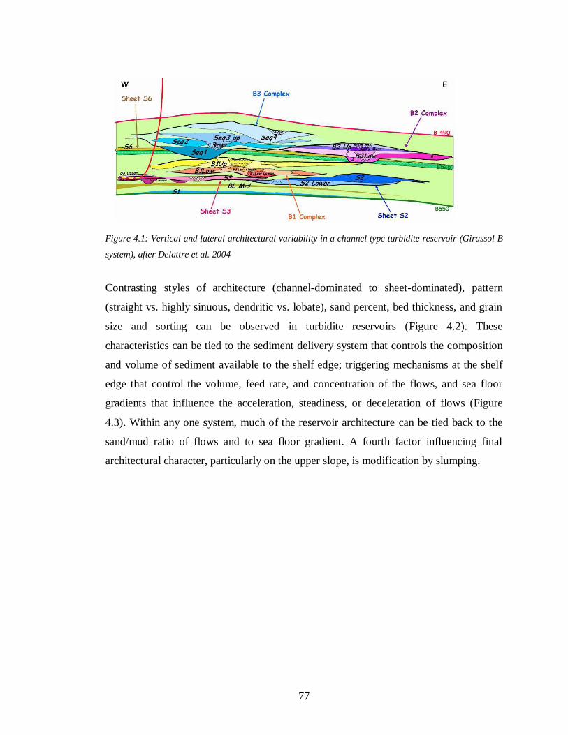
77

Figure 4.1: Vertical and lateral architectural variability in a channel type turbidite reservoir (Girassol B

system), after Delattre et al. 2004

Contrasting styles of architecture (channel-dominated to sheet-dominated), pattern

(straight vs. highly sinuous, dendritic vs. lobate), sand percent, bed thickness, and grain

size and sorting can be observed in turbidite reservoirs (Figure 4.2). These

characteristics can be tied to the sediment delivery system that controls the composition

and volume of sediment available to the shelf edge; triggering mechanisms at the shelf

edge that control the volume, feed rate, and concentration of the flows, and sea floor

gradients that influence the acceleration, steadiness, or deceleration of flows (Figure

4.3). Within any one system, much of the reservoir architecture can be tied back to the

sand/mud ratio of flows and to sea floor gradient. A fourth factor influencing final

architectural character, particularly on the upper slope, is modification by slumping.

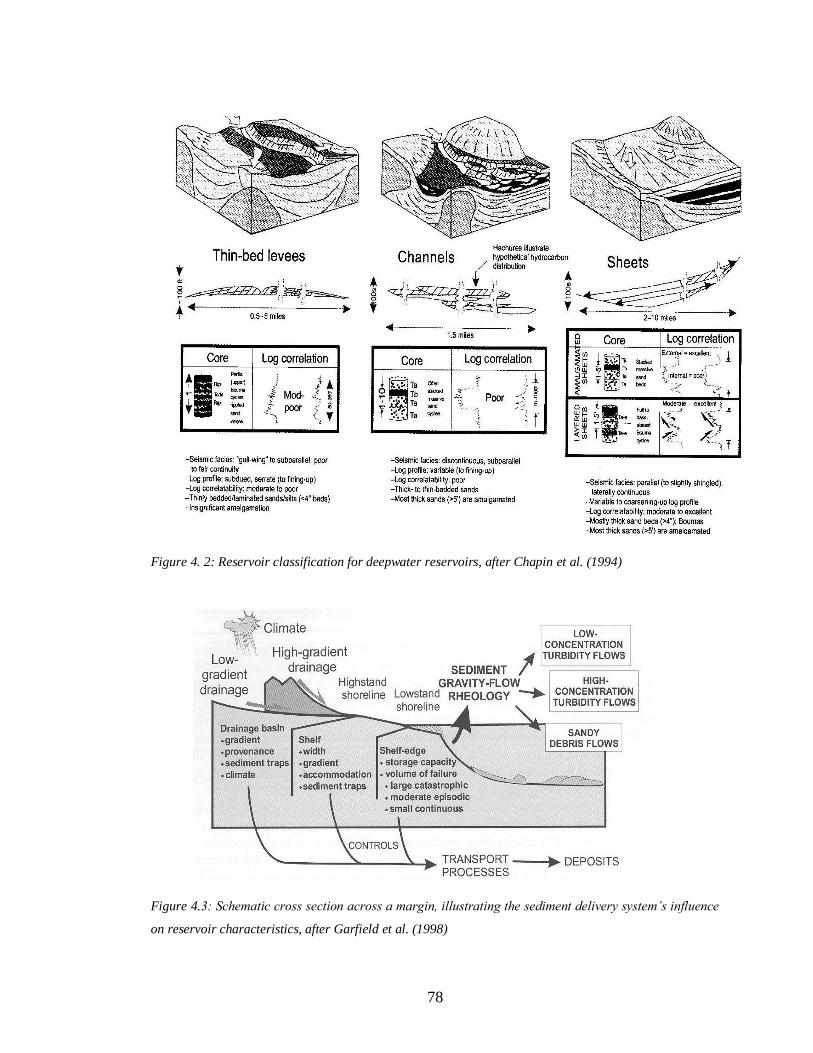
78

Figure 4. 2: Reservoir classification for deepwater reservoirs, after Chapin et al. (1994)

Figure 4.3: Schematic cross section across a margin, illustrating the sediment delivery system’s influence

on reservoir characteristics, after Garfield et al. (1998)

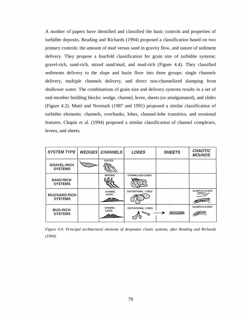
79

A number of papers have identified and classified the basic controls and properties of

turbidite deposits. Reading and Richards (1994) proposed a classification based on two

primary controls: the amount of mud versus sand in gravity flow, and nature of sediment

delivery. They propose a fourfold classification for grain size of turbidite systems:

gravel-rich, sand-rich, mixed sand/mud, and mud-rich (Figure 4.4). They classified

sediments delivery to the slope and basin floor into three groups: single channels

delivery, multiple channels delivery, and direct non-channelized slumping from

shallower water. The combinations of grain size and delivery systems results in a set of

end-member building blocks: wedge, channel, levee, sheets (or amalgamated), and slides

(Figure 4.2). Mutti and Normark (1987 and 1991) proposed a similar classification of

turbidite elements: channels, overbanks, lobes, channel-lobe transition, and erosional

features. Chapin et al. (1994) proposed a similar classification of channel complexes,

levees, and sheets.

Figure 4.4: Principal architectural elements of deepwater clastic systems, after Reading and Richards

(1994).

80

4.3 Challenges in turbidite reservoirs management

In general, the size and geometry of a turbidite reservoir and its internal sand distribution

are properties that control ultimate reservoir recovery. Large scale features, like laterally

continuous, thick, permeable sands can be determined from seismic attributes, well logs,

and well test and production data.

Many problems in turbidite reservoir development; such as early water breakthrough,

abrupt reservoir pressure drops, and gas coning; arise from more subtle, subseismic scale

properties (Weimer et al., 2000a). Subseismic scale properties, which are beneath the

vertical resolution of conventional 3D seismic-reflection data, exert strong control on

individual well production rates and ultimate recoveries. Features such as lateral bed

continuity, vertical bed connectivity, reservoir quality, and net sand content normally

cannot be determined from seismic images, yet these are the features that control fluid

flow within the reservoir. Also, small-offset faults and fractures, which are common and

critical components of reservoirs, cannot be imaged by conventional seismic. Newer

techniques, such as spectral decomposition and PSDM, are improving our ability to

detect small-scale stratigraphic and structural compartments; however, there still are the

natural physical limits to the resolution of seismic images.

The major architectural elements that form the bulk of turbidite reservoirs are channel-

fills, sheets and lobes, and overbank/levees. Although these elements can be recognized

on seismic profiles and wireline logs, internal variability exists within each element that

can affect reservoir performance. Table 4.1 lists the qualitative attributes of continuity,

connectivity, and reservoir quality as they are present within each of these elements.

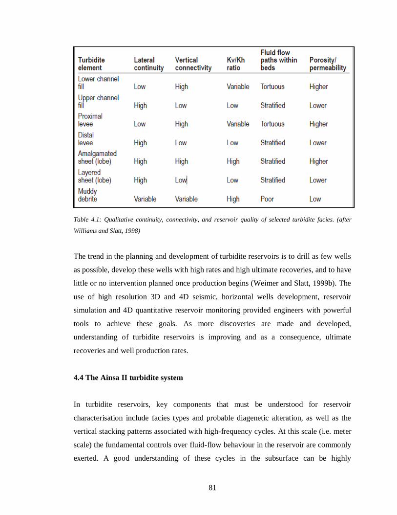
81

Table 4.1: Qualitative continuity, connectivity, and reservoir quality of selected turbidite facies. (after

Williams and Slatt, 1998)

The trend in the planning and development of turbidite reservoirs is to drill as few wells

as possible, develop these wells with high rates and high ultimate recoveries, and to have

little or no intervention planned once production begins (Weimer and Slatt, 1999b). The

use of high resolution 3D and 4D seismic, horizontal wells development, reservoir

simulation and 4D quantitative reservoir monitoring provided engineers with powerful

tools to achieve these goals. As more discoveries are made and developed,

understanding of turbidite reservoirs is improving and as a consequence, ultimate

recoveries and well production rates.

4.4 The Ainsa II turbidite system

In turbidite reservoirs, key components that must be understood for reservoir

characterisation include facies types and probable diagenetic alteration, as well as the

vertical stacking patterns associated with high-frequency cycles. At this scale (i.e. meter

scale) the fundamental controls over fluid-flow behaviour in the reservoir are commonly

exerted. A good understanding of these cycles in the subsurface can be highly

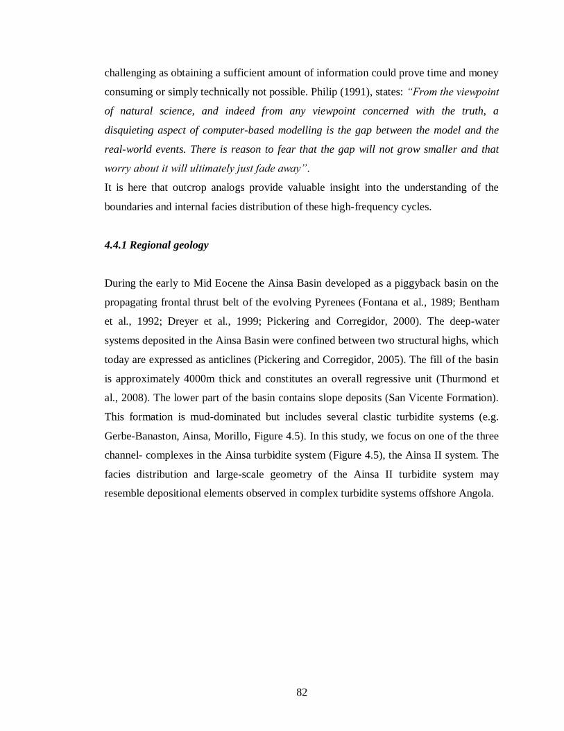
82

challenging as obtaining a sufficient amount of information could prove time and money

consuming or simply technically not possible. Philip (1991), states: “From the viewpoint

of natural science, and indeed from any viewpoint concerned with the truth, a

disquieting aspect of computer-based modelling is the gap between the model and the

real-world events. There is reason to fear that the gap will not grow smaller and that

worry about it will ultimately just fade away”.

It is here that outcrop analogs provide valuable insight into the understanding of the

boundaries and internal facies distribution of these high-frequency cycles.

4.4.1 Regional geology

During the early to Mid Eocene the Ainsa Basin developed as a piggyback basin on the

propagating frontal thrust belt of the evolving Pyrenees (Fontana et al., 1989; Bentham

et al., 1992; Dreyer et al., 1999; Pickering and Corregidor, 2000). The deep-water

systems deposited in the Ainsa Basin were confined between two structural highs, which

today are expressed as anticlines (Pickering and Corregidor, 2005). The fill of the basin

is approximately 4000m thick and constitutes an overall regressive unit (Thurmond et

al., 2008). The lower part of the basin contains slope deposits (San Vicente Formation).

This formation is mud-dominated but includes several clastic turbidite systems (e.g.

Gerbe-Banaston, Ainsa, Morillo, Figure 4.5). In this study, we focus on one of the three

channel- complexes in the Ainsa turbidite system (Figure 4.5), the Ainsa II system. The

facies distribution and large-scale geometry of the Ainsa II turbidite system may

resemble depositional elements observed in complex turbidite systems offshore Angola.

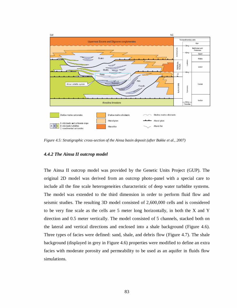
83

Figure 4.5: Stratigraphic cross-section of the Ainsa basin deposit (after Bakke et al., 2007)

4.4.2 The Ainsa II outcrop model

The Ainsa II outcrop model was provided by the Genetic Units Project (GUP). The

original 2D model was derived from an outcrop photo-panel with a special care to

include all the fine scale heterogeneities characteristic of deep water turbidite systems.

The model was extended to the third dimension in order to perform fluid flow and

seismic studies. The resulting 3D model consisted of 2,600,000 cells and is considered

to be very fine scale as the cells are 5 meter long horizontally, in both the X and Y

direction and 0.5 meter vertically. The model consisted of 5 channels, stacked both on

the lateral and vertical directions and enclosed into a shale background (Figure 4.6).

Three types of facies were defined: sand, shale, and debris flow (Figure 4.7). The shale

background (displayed in grey in Figure 4.6) properties were modified to define an extra

facies with moderate porosity and permeability to be used as an aquifer in fluids flow

simulations.

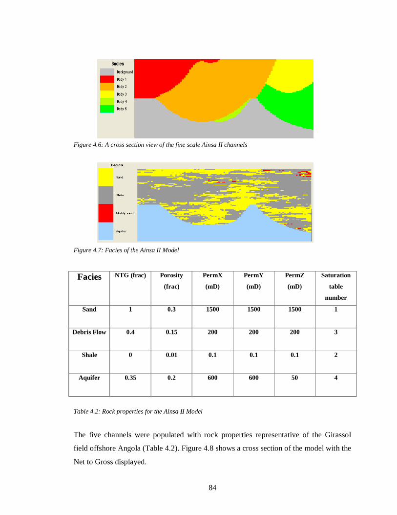
84

Figure 4.6: A cross section view of the fine scale Ainsa II channels

Figure 4.7: Facies of the Ainsa II Model

Facies NTG (frac) Porosity

(frac)

PermX

(mD)

PermY

(mD)

PermZ

(mD)

Saturation

table

number

Sand

1 0.3 1500 1500 1500 1

Debris Flow

0.4 0.15 200 200 200 3

Shale

0 0.01 0.1 0.1 0.1 2

Aquifer

0.35 0.2 600 600 50 4

Table 4.2: Rock properties for the Ainsa II Model

The five channels were populated with rock properties representative of the Girassol

field offshore Angola (Table 4.2). Figure 4.8 shows a cross section of the model with the

Net to Gross displayed.

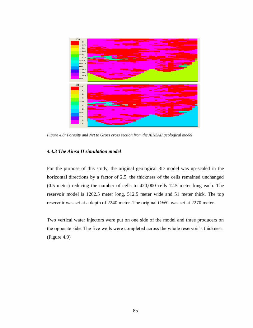
85

Figure 4.8: Porosity and Net to Gross cross section from the AINSAII geological model

4.4.3 The Ainsa II simulation model

For the purpose of this study, the original geological 3D model was up-scaled in the

horizontal directions by a factor of 2.5, the thickness of the cells remained unchanged

(0.5 meter) reducing the number of cells to 420,000 cells 12.5 meter long each. The

reservoir model is 1262.5 meter long, 512.5 meter wide and 51 meter thick. The top

reservoir was set at a depth of 2240 meter. The original OWC was set at 2270 meter.

Two vertical water injectors were put on one side of the model and three producers on

the opposite side. The five wells were completed across the whole reservoir’s thickness.

(Figure 4.9)

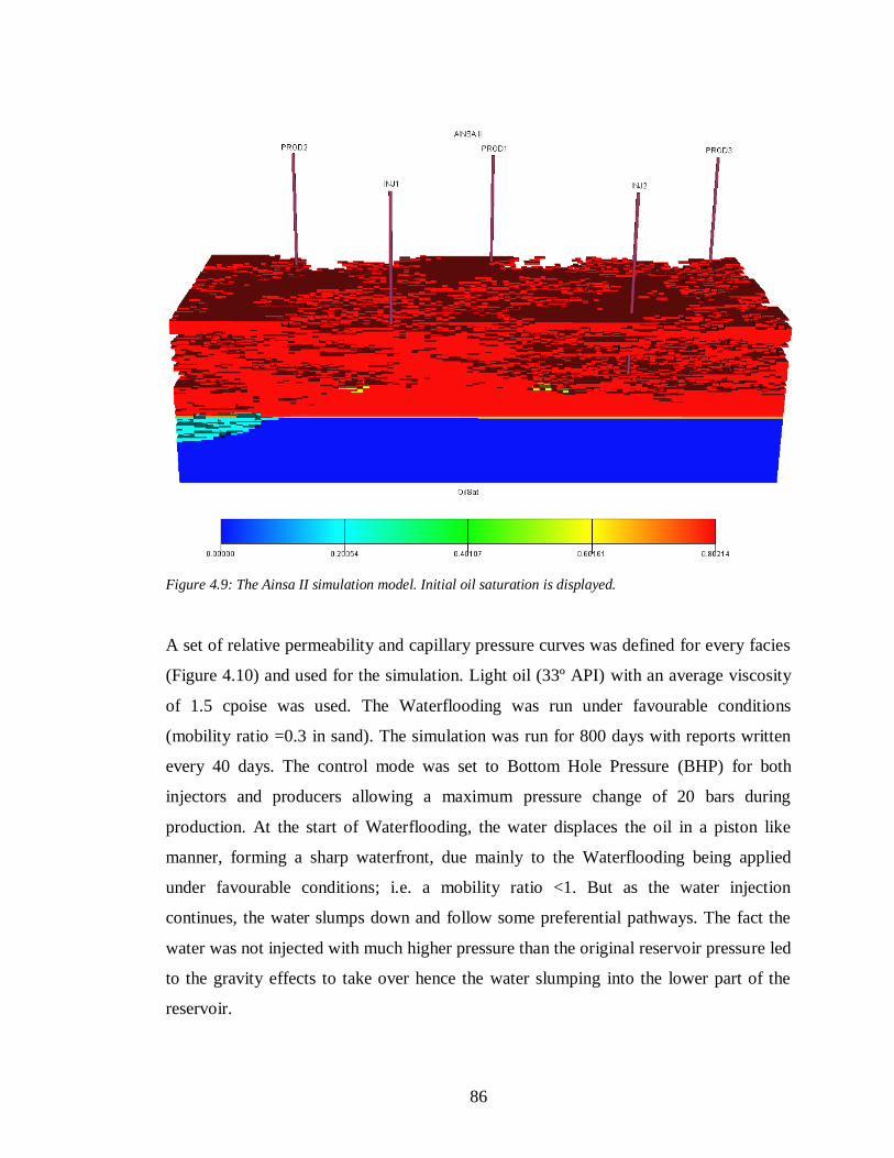
86

Figure 4.9: The Ainsa II simulation model. Initial oil saturation is displayed.

A set of relative permeability and capillary pressure curves was defined for every facies

(Figure 4.10) and used for the simulation. Light oil (33º API) with an average viscosity

of 1.5 cpoise was used. The Waterflooding was run under favourable conditions

(mobility ratio =0.3 in sand). The simulation was run for 800 days with reports written

every 40 days. The control mode was set to Bottom Hole Pressure (BHP) for both

injectors and producers allowing a maximum pressure change of 20 bars during

production. At the start of Waterflooding, the water displaces the oil in a piston like

manner, forming a sharp waterfront, due mainly to the Waterflooding being applied

under favourable conditions; i.e. a mobility ratio <1. But as the water injection

continues, the water slumps down and follow some preferential pathways. The fact the

water was not injected with much higher pressure than the original reservoir pressure led

to the gravity effects to take over hence the water slumping into the lower part of the

reservoir.

87

Figure 4.10: Relative permeability and capillary pressure curves used in the simulation

Figure 4.11 shows the oil saturation in a cross-section of the reservoir model, where the

water injector INJ1 was placed, at different time steps of the Waterflooding. Figure

4.11-a shows the original oil saturation (before production), 4.11-b after 40 days, 4.11-c

after 200 days and 4.11-d after 800 days.

88

a b

c d

Figure 4.11: Oil Saturation before the start of production, after 40 days, 200 days and 800 days of

Waterflooding

The shale cells were defined as inactive cells in the simulation model meaning that there

is no fluids flow in the shale. The water flow is affected by those intra-reservoir shales

and develops a complex waterfront directly linked to the facies distribution in the model

Figure 4.12 shows the facies at the two water injectors INJ1 and INJ2 locations. It is

clear that the injector INJ1 is more efficient in displacing oil toward the producers as it

is completed across several high pay layers, while the well INJ2 will be injecting mainly

in the aquifer. Lateral connectivity also has a major impact as of the radius of influence

of the two wells.

89

Figure 4.12: Facies and Net to Gross distribution at water injector wells INJ1 and INJ2 locations.

Figure 4.13 shows facies distribution at different layers of the reservoir model. The

yellow colour represents the sand and the channelized nature of the reservoir is clearly

shown. The lateral connectivity between the different wells in the model is highly

variable with depth, resulting in a highly heterogeneous waterfront both in the vertical

and lateral direction. Our study aims at understanding the 4D signatures of such complex

waterfront.

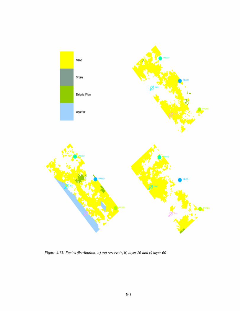
90

Figure 4.13: Facies distribution: a) top reservoir, b) layer 26 and c) layer 60

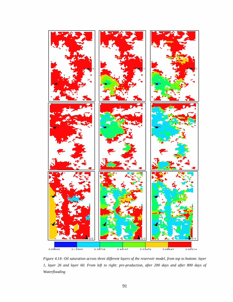
91

Figure 4.14: Oil saturation across three different layers of the reservoir model, from top to bottom: layer

1, layer 26 and layer 60. From left to right: pre-production, after 200 days and after 800 days of

Waterflooding

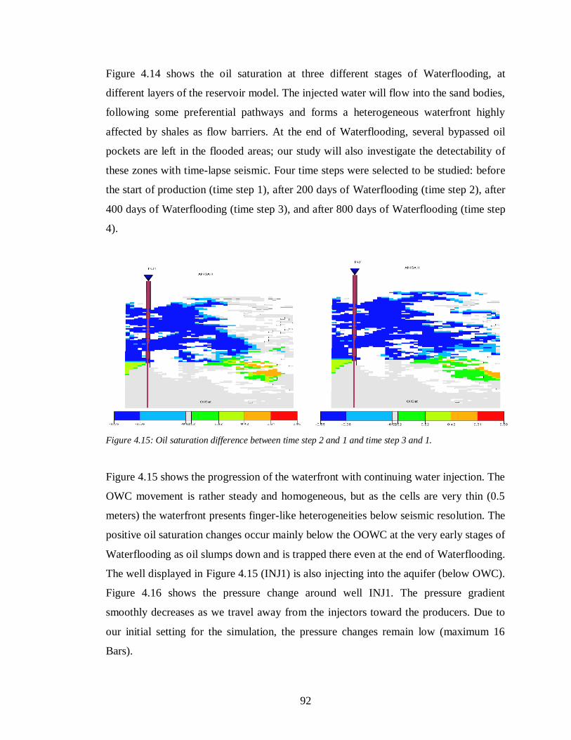
92

Figure 4.14 shows the oil saturation at three different stages of Waterflooding, at

different layers of the reservoir model. The injected water will flow into the sand bodies,

following some preferential pathways and forms a heterogeneous waterfront highly

affected by shales as flow barriers. At the end of Waterflooding, several bypassed oil

pockets are left in the flooded areas; our study will also investigate the detectability of

these zones with time-lapse seismic. Four time steps were selected to be studied: before

the start of production (time step 1), after 200 days of Waterflooding (time step 2), after

400 days of Waterflooding (time step 3), and after 800 days of Waterflooding (time step

4).

Figure 4.15: Oil saturation difference between time step 2 and 1 and time step 3 and 1.

Figure 4.15 shows the progression of the waterfront with continuing water injection. The

OWC movement is rather steady and homogeneous, but as the cells are very thin (0.5

meters) the waterfront presents finger-like heterogeneities below seismic resolution. The

positive oil saturation changes occur mainly below the OOWC at the very early stages of

Waterflooding as oil slumps down and is trapped there even at the end of Waterflooding.

The well displayed in Figure 4.15 (INJ1) is also injecting into the aquifer (below OWC).

Figure 4.16 shows the pressure change around well INJ1. The pressure gradient

smoothly decreases as we travel away from the injectors toward the producers. Due to

our initial setting for the simulation, the pressure changes remain low (maximum 16

Bars).

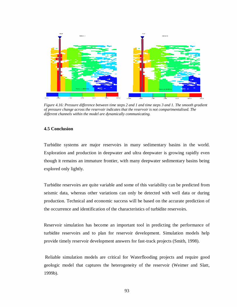
93

Figure 4.16: Pressure difference between time steps 2 and 1 and time steps 3 and 1. The smooth gradient

of pressure change across the reservoir indicates that the reservoir is not compartmentalised. The

different channels within the model are dynamically communicating.

4.5 Conclusion

Turbidite systems are major reservoirs in many sedimentary basins in the world.

Exploration and production in deepwater and ultra deepwater is growing rapidly even

though it remains an immature frontier, with many deepwater sedimentary basins being

explored only lightly.

Turbidite reservoirs are quite variable and some of this variability can be predicted from

seismic data, whereas other variations can only be detected with well data or during

production. Technical and economic success will be based on the accurate prediction of

the occurrence and identification of the characteristics of turbidite reservoirs.

Reservoir simulation has become an important tool in predicting the performance of

turbidite reservoirs and to plan for reservoir development. Simulation models help

provide timely reservoir development answers for fast-track projects (Smith, 1998).

Reliable simulation models are critical for Waterflooding projects and require good

geologic model that captures the heterogeneity of the reservoir (Weimer and Slatt,

1999b).

94

Quantifying the heterogeneity of turbidite reservoirs for simulation is difficult and

accounts for the use of geostatistical models. Continuity of gross turbidite intervals can

be obtained from 3-D seismic horizon slices, as well as from interference and pressure

tests. Quantification of bed thickness, connectivity, and reservoir quality can be

accomplished from well information, but accurate prediction of these features away

from the well is not wholly reliable using conventional wireline logs. Subtle features on

dipmeter logs or borehole imaging tools may provide information on lateral attributes.

Outcrops, where sufficiently continuous, can provide the necessary quantitative lateral

attributes of turbidite strata and can bridge the gap between wireline log and seismic

scales.

An outcrop based reservoir model was built to simulate Waterflooding in turbidite

reservoirs. The fluid flow simulation showed that the water will flow in some

preferential pathways controlled by the reservoir internal geology. Permeability values

and NTG distribution play a major role in the advance of the waterfront inside the

reservoir and control its shape and location. Indeed, reservoir heterogeneities create a

fractal-like waterfront surface that can vary greatly across the reservoir, both

horizontally and vertically. Waterflooding simulation in a highly heterogeneous turbidite

clearly showed the critical impact reservoir’s heterogeneities (heterogeneous

permeability and net-to-gross distribution) on sweep efficiency and recovery factors. By

the end of the Waterflooding simulation, 80% of the oil in place is recovered, but the

injection of several pore volumes of water was necessary to achieve this recovery factor,

mainly due to the reservoir internal heterogeneities.

95

Chapter 5

Numerical modelling of Waterflooding in turbidite reservoirs and

simulator to seismic study

In this chapter, petrophysical simulation results performed on the AINSAII simulation

model output are discussed. Synthetic seismic was created for a set of three different

dominant frequencies. Interpretation of 3D and 4D seismic signatures of Waterflooding

is carried out on each seismic set. Resolution issues were addressed.

96

5.1 Introduction

Geoscientists share a common interest in investigating and characterizing the geological

subsurface as accurately as possible. Hydrocarbon reservoirs are generally composed of

irregular geological units with distinguishing characteristics. The boundaries between

units create discontinuities that are further complicated by faulting, erosion and

deposition. Within this heterogeneous complexity, geoscientists aim to develop a good

understanding of the geological setting of the reservoir of interest.

Due to the limitation on the amount of information available to geoscientists in order to

develop such an understanding, computer modelling is used to build geological models

integrating all the available data and being as representative as possible of the real

conditions in the subsurface. The accuracy of the geological model is crucial in the sense

that these models are up-scaled in a later stage in order to simulate fluids flow within the

reservoir as a tool to forecast future performance of the reservoir, a valuable tool in the

assessing of the efficiency of the production scenarios proposed and gives a good

estimate of the possible cost of such scenarios.

The development of a geologically constrained reservoir model and subsequent up-

scaling of the model for reservoir simulation depends on critical input parameters

defining both the geometrical attributes and distribution of the targeted facies.

Integration of geologically based elements is a fundamental step in the characterisation

of the probable vertical and lateral distribution of reservoir facies in the subsurface. Such

a geologically based model will increase our understanding of reservoir heterogeneit ies

and provides the foundation to build accurate simulation models.

In this study, an outcrop model was used to address uncertainty in recovery and sweep

efficiency of Waterflooding in deep-water channelized reservoirs. Three dimensional

heterogeneities were added to the outcrop model as they are of high importance for flow

simulation and seismic studies. The results from the flow simulation were used in the

petrophysical modelling to compute values of Vp, Vs and Rho at different time steps and

97

in every grid cell. 3D Synthetic seismic cubes were created for 4 time steps

corresponding to 4 different stages of Waterflooding. 3 different dominating seismic

frequencies were modelled in order to investigate the effects of seismic resolution on the

interpretation of the time lapse signature of Waterflooding in geologically complex

turbidite reservoirs.

5.2 Petro-elastic modelling results

Gassmann (1958), Batzle and Wang (1992) and MacBeth (2005) equations were used in

the transformation from the engineering domain (pressure and saturations distributions

across the reservoir) to the petro-elastic domain (Vp, Vs and Rho).

Figure 5.1 shows the relative changes in density, P-wave and S-wave velocities and

impedances after 200 and 800 days of Waterflooding. The displayed cross-section is

extracted at one water injection well location. The magnitude of changes was the same

after 200 days and 800 days of Waterflooding; i.e. the maximum P-wave velocity (for

example) was 4% at the two time steps. The percentage of change is directly linked to

the water saturation change in the reservoir. As the water is injected into the reservoir, it

pushes away the oil and occupies the vacant pore volume left when the oil has moved.

The changes from a fully oil saturated rock to a fully water saturated rock (irreducible

saturations ) happens gradually and not all the saturation changes are visible after the

petro-elastic transformation.

The changes in P-wave velocity and density follow the same patterns; positive changes

in the areas where water saturation increased and negative change where water

saturation decreased. These changes are mainly controlled by the changes in fluids

saturations rather than pressure; this is particularly visible on the density cubes. This

could be explained by the fact that the pressure change, in the absence of any

compartmentalisation within the reservoir, is not localised on a particular location inside

the reservoir, but it is fairly smooth. Its effect is rather global and would result in a

―dimming‖ or decrease in the magnitude of changes observed in P-wave and density

cubes.

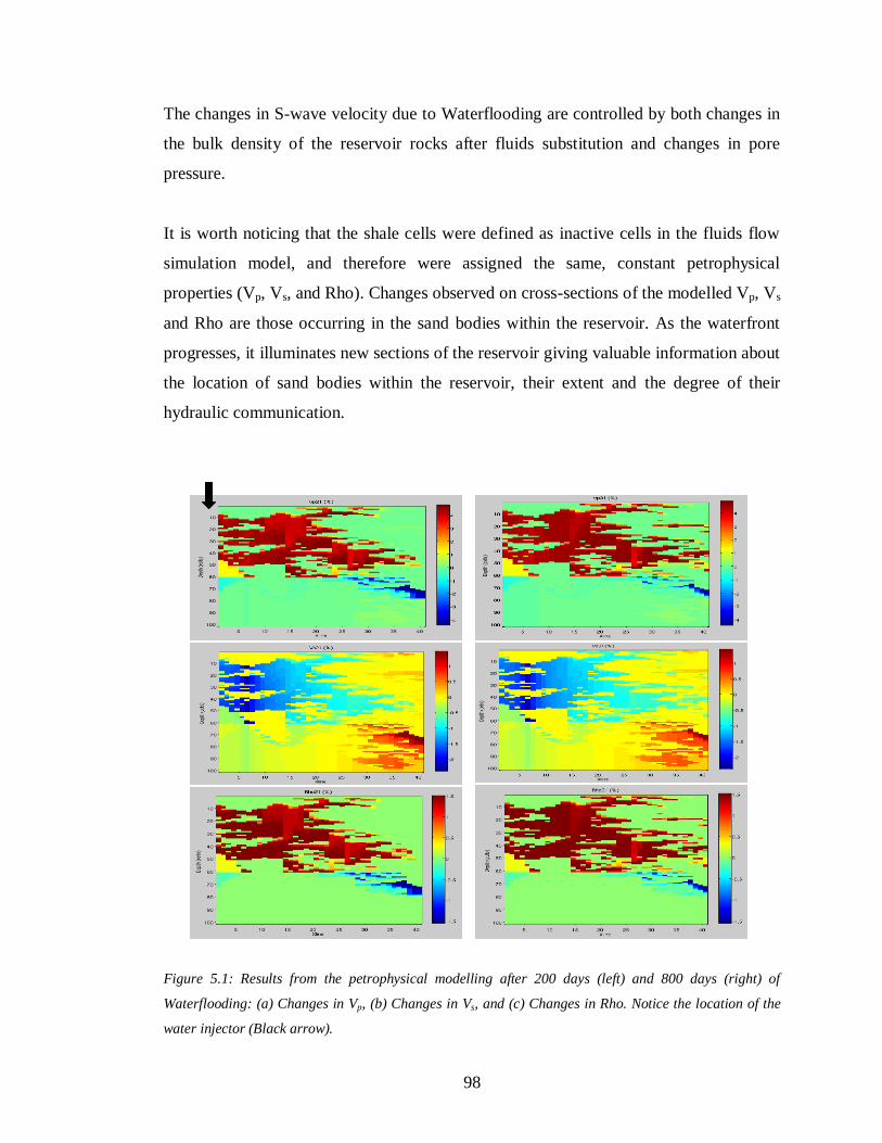
98

The changes in S-wave velocity due to Waterflooding are controlled by both changes in

the bulk density of the reservoir rocks after fluids substitution and changes in pore

pressure.

It is worth noticing that the shale cells were defined as inactive cells in the fluids flow

simulation model, and therefore were assigned the same, constant petrophysical

properties (Vp, Vs, and Rho). Changes observed on cross-sections of the modelled Vp, Vs

and Rho are those occurring in the sand bodies within the reservoir. As the waterfront

progresses, it illuminates new sections of the reservoir giving valuable information about

the location of sand bodies within the reservoir, their extent and the degree of their

hydraulic communication.

Figure 5.1: Results from the petrophysical modelling after 200 days (left) and 800 days (right) of

Waterflooding: (a) Changes in Vp, (b) Changes in Vs, and (c) Changes in Rho. Notice the location of the

water injector (Black arrow).

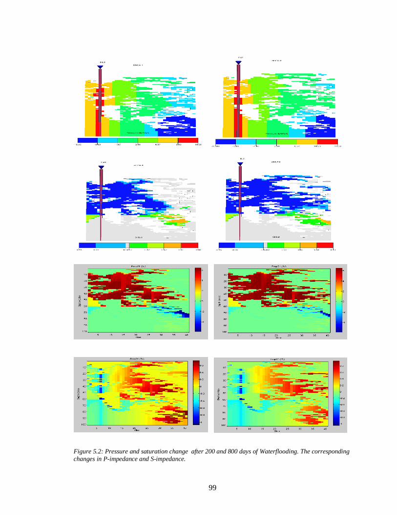
99

Figure 5.2: Pressure and saturation change after 200 and 800 days of Waterflooding. The corresponding

changes in P-impedance and S-impedance.

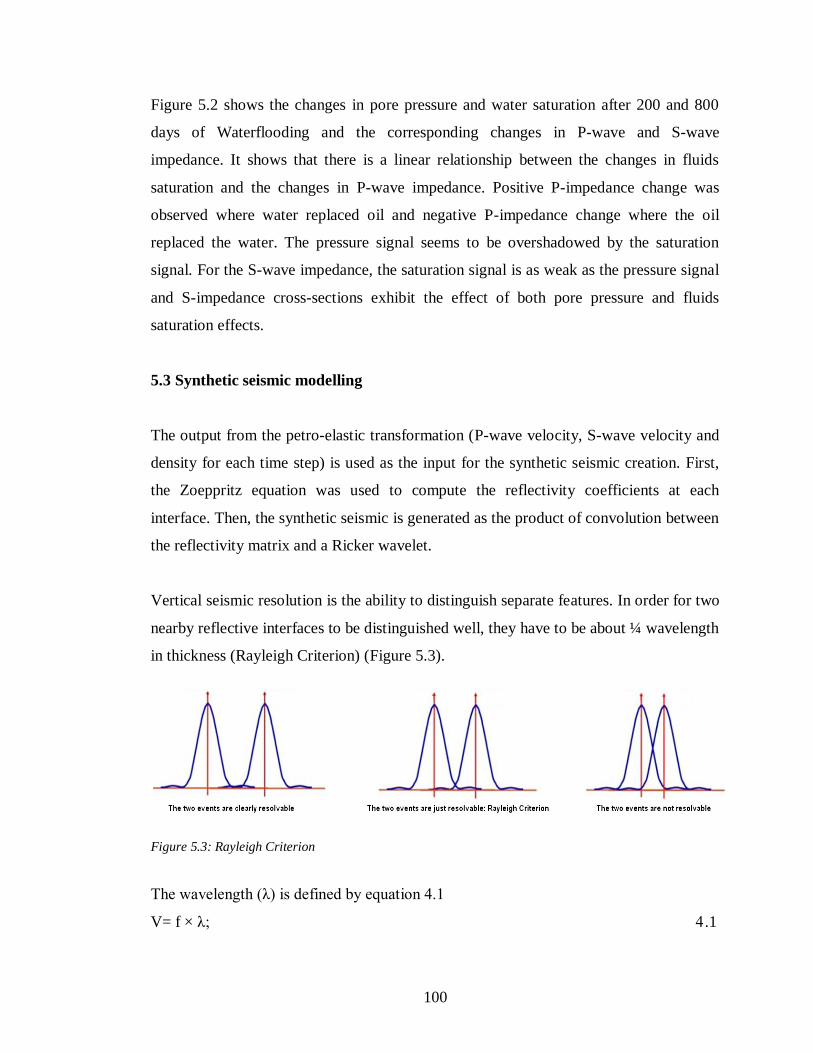
100

Figure 5.2 shows the changes in pore pressure and water saturation after 200 and 800

days of Waterflooding and the corresponding changes in P-wave and S-wave

impedance. It shows that there is a linear relationship between the changes in fluids

saturation and the changes in P-wave impedance. Positive P-impedance change was

observed where water replaced oil and negative P-impedance change where the oil

replaced the water. The pressure signal seems to be overshadowed by the saturation

signal. For the S-wave impedance, the saturation signal is as weak as the pressure signal

and S-impedance cross-sections exhibit the effect of both pore pressure and fluids

saturation effects.

5.3 Synthetic seismic modelling

The output from the petro-elastic transformation (P-wave velocity, S-wave velocity and

density for each time step) is used as the input for the synthetic seismic creation. First,

the Zoeppritz equation was used to compute the reflectivity coefficients at each

interface. Then, the synthetic seismic is generated as the product of convolution between

the reflectivity matrix and a Ricker wavelet.

Vertical seismic resolution is the ability to distinguish separate features. In order for two

nearby reflective interfaces to be distinguished well, they have to be about ¼ wavelength

in thickness (Rayleigh Criterion) (Figure 5.3).

Figure 5.3: Rayleigh Criterion

The wavelength (λ) is defined by equation 4.1

V= f × λ; 4 .1

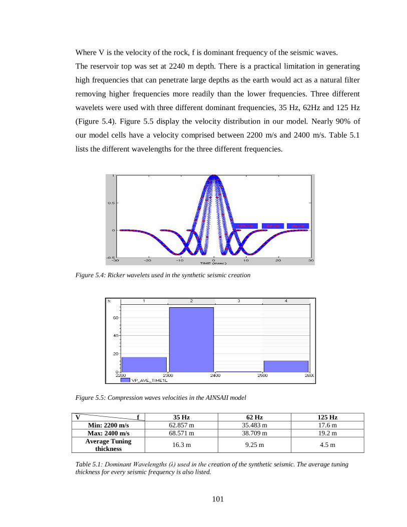
101

Where V is the velocity of the rock, f is dominant frequency of the seismic waves.

The reservoir top was set at 2240 m depth. There is a practical limitation in generating

high frequencies that can penetrate large depths as the earth would act as a natural filter

removing higher frequencies more readily than the lower frequencies. Three different

wavelets were used with three different dominant frequencies, 35 Hz, 62Hz and 125 Hz

(Figure 5.4). Figure 5.5 display the velocity distribution in our model. Nearly 90% of

our model cells have a velocity comprised between 2200 m/s and 2400 m/s. Table 5.1

lists the different wavelengths for the three different frequencies.

Figure 5.4: Ricker wavelets used in the synthetic seismic creation

Figure 5.5: Compression waves velocities in the AINSAII model

V f 35 Hz 62 Hz 125 Hz

Min: 2200 m/s 62.857 m 35.483 m 17.6 m

Max: 2400 m/s 68.571 m 38.709 m 19.2 m

Average Tuning

thickness 16.3 m 9.25 m 4.5 m

Table 5.1: Dominant Wavelengths (λ) used in the creation of the synthetic seismic. The average tuning

thickness for every seismic frequency is also listed.

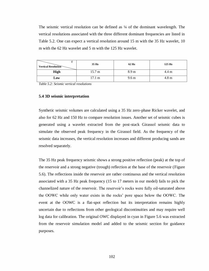
102

The seismic vertical resolution can be defined as ¼ of the dominant wavelength. The

vertical resolutions associated with the three different dominant frequencies are listed in

Table 5.2. One can expect a vertical resolution around 15 m with the 35 Hz wavelet, 10

m with the 62 Hz wavelet and 5 m with the 125 Hz wavelet.

f

Vertical Resolution 35 Hz 62 Hz 125 Hz

High 15.7 m 8.9 m 4.4 m

Low 17.1 m 9.6 m 4.8 m

Table 5.2: Seismic vertical resolutions

5.4 3D seismic interpretation

Synthetic seismic volumes are calculated using a 35 Hz zero-phase Ricker wavelet, and

also for 62 Hz and 150 Hz to compare resolution issues. Another set of seismic cubes is

generated using a wavelet extracted from the post-stack Girassol seismic data to

simulate the observed peak frequency in the Girassol field. As the frequency of the

seismic data increases, the vertical resolution increases and different producing sands are

resolved separately.

The 35 Hz peak frequency seismic shows a strong positive reflection (peak) at the top of

the reservoir and a strong negative (trough) reflection at the base of the reservoir (Figure

5.6). The reflections inside the reservoir are rather continuous and the vertical resolution

associated with a 35 Hz peak frequency (15 to 17 meters in our model) fails to pick the

channelized nature of the reservoir. The reservoir’s rocks were fully oil-saturated above

the OOWC while only water exists in the rocks’ pore space below the OOWC. The

event at the OOWC is a flat-spot reflection but its interpretation remains highly

uncertain due to reflections from other geological discontinuities and may require well

log data for calibration. The original OWC displayed in cyan in Figure 5.6 was extracted

from the reservoir simulation model and added to the seismic section for guidance

purposes.

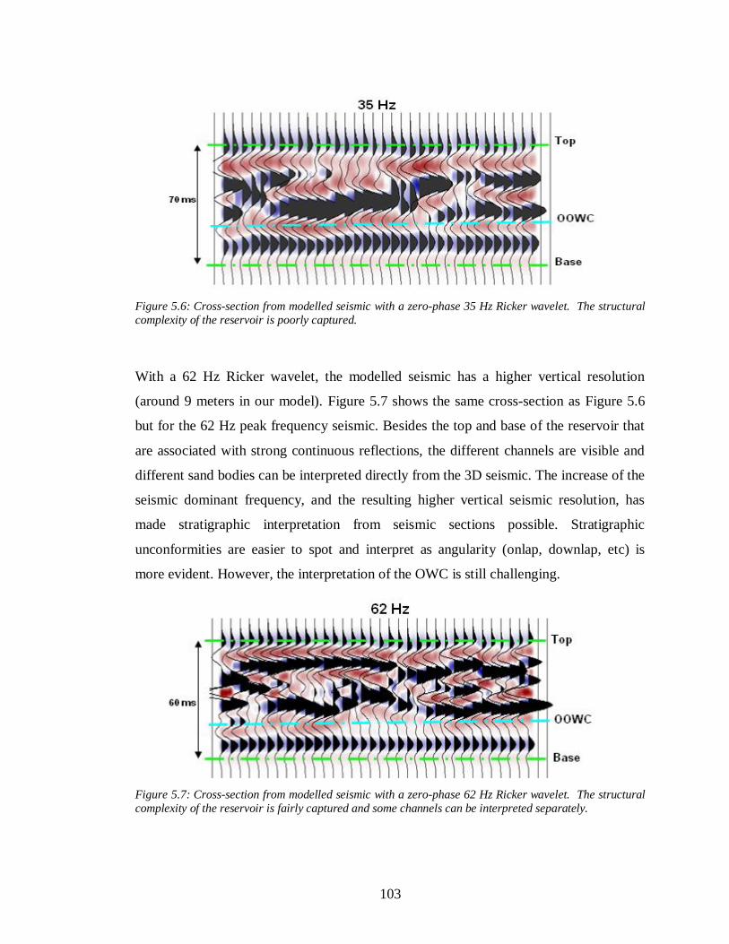
103

Figure 5.6: Cross-section from modelled seismic with a zero-phase 35 Hz Ricker wavelet. The structural

complexity of the reservoir is poorly captured.

With a 62 Hz Ricker wavelet, the modelled seismic has a higher vertical resolution

(around 9 meters in our model). Figure 5.7 shows the same cross-section as Figure 5.6

but for the 62 Hz peak frequency seismic. Besides the top and base of the reservoir that

are associated with strong continuous reflections, the different channels are visible and

different sand bodies can be interpreted directly from the 3D seismic. The increase of the

seismic dominant frequency, and the resulting higher vertical seismic resolution, has

made stratigraphic interpretation from seismic sections possible. Stratigraphic

unconformities are easier to spot and interpret as angularity (onlap, downlap, etc) is

more evident. However, the interpretation of the OWC is still challenging.


complexity of the reservoir is fairly captured and some channels can be interpreted separately.

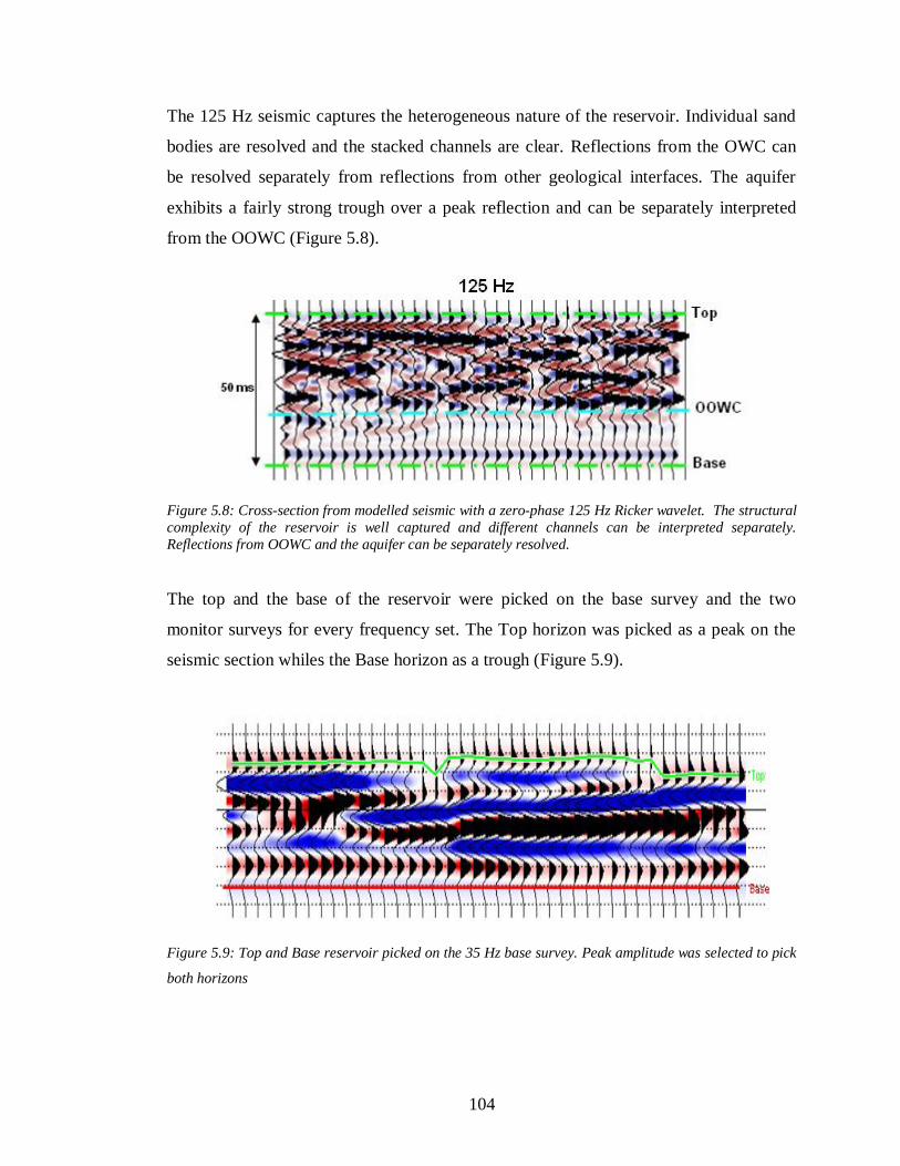
104

The 125 Hz seismic captures the heterogeneous nature of the reservoir. Individual sand

bodies are resolved and the stacked channels are clear. Reflections from the OWC can

be resolved separately from reflections from other geological interfaces. The aquifer

exhibits a fairly strong trough over a peak reflection and can be separately interpreted

from the OOWC (Figure 5.8).


complexity of the reservoir is well captured and different channels can be interpreted separately.

Reflections from OOWC and the aquifer can be separately resolved.

The top and the base of the reservoir were picked on the base survey and the two

monitor surveys for every frequency set. The Top horizon was picked as a peak on the

seismic section whiles the Base horizon as a trough (Figure 5.9).

Figure 5.9: Top and Base reservoir picked on the 35 Hz base survey. Peak amplitude was selected to pick

both horizons

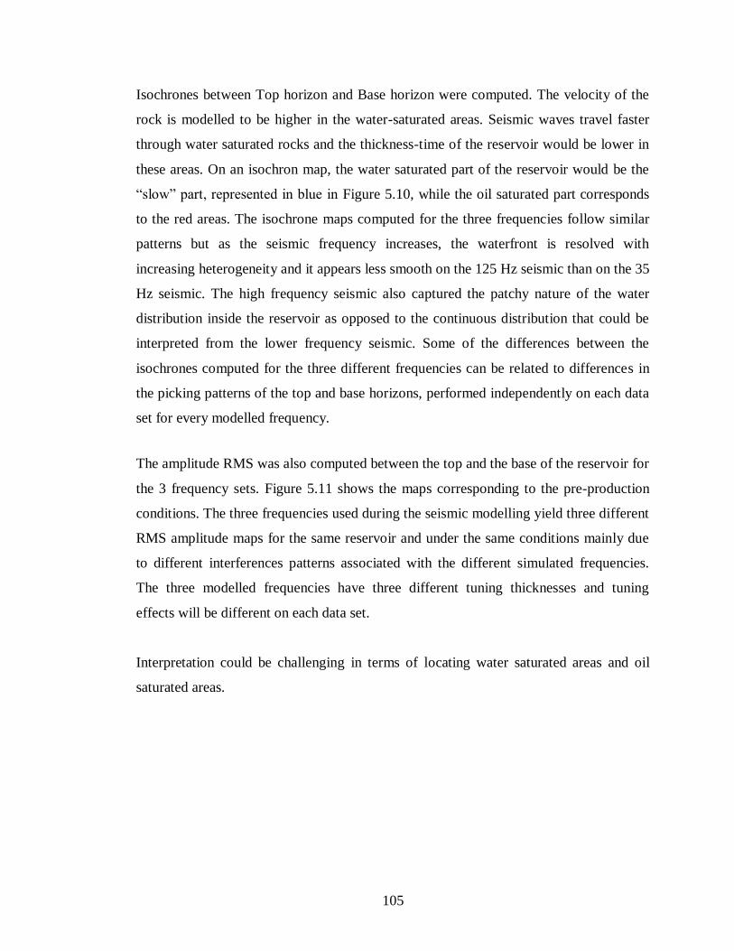
105

Isochrones between Top horizon and Base horizon were computed. The velocity of the

rock is modelled to be higher in the water-saturated areas. Seismic waves travel faster

through water saturated rocks and the thickness-time of the reservoir would be lower in

these areas. On an isochron map, the water saturated part of the reservoir would be the

―slow‖ part, represented in blue in Figure 5.10, while the oil saturated part corresponds

to the red areas. The isochrone maps computed for the three frequencies follow similar

patterns but as the seismic frequency increases, the waterfront is resolved with

increasing heterogeneity and it appears less smooth on the 125 Hz seismic than on the 35

Hz seismic. The high frequency seismic also captured the patchy nature of the water

distribution inside the reservoir as opposed to the continuous distribution that could be

interpreted from the lower frequency seismic. Some of the differences between the

isochrones computed for the three different frequencies can be related to differences in

the picking patterns of the top and base horizons, performed independently on each data

set for every modelled frequency.

The amplitude RMS was also computed between the top and the base of the reservoir for

the 3 frequency sets. Figure 5.11 shows the maps corresponding to the pre-production

conditions. The three frequencies used during the seismic modelling yield three different

RMS amplitude maps for the same reservoir and under the same conditions mainly due

to different interferences patterns associated with the different simulated frequencies.

The three modelled frequencies have three different tuning thicknesses and tuning

effects will be different on each data set.

Interpretation could be challenging in terms of locating water saturated areas and oil

saturated areas.

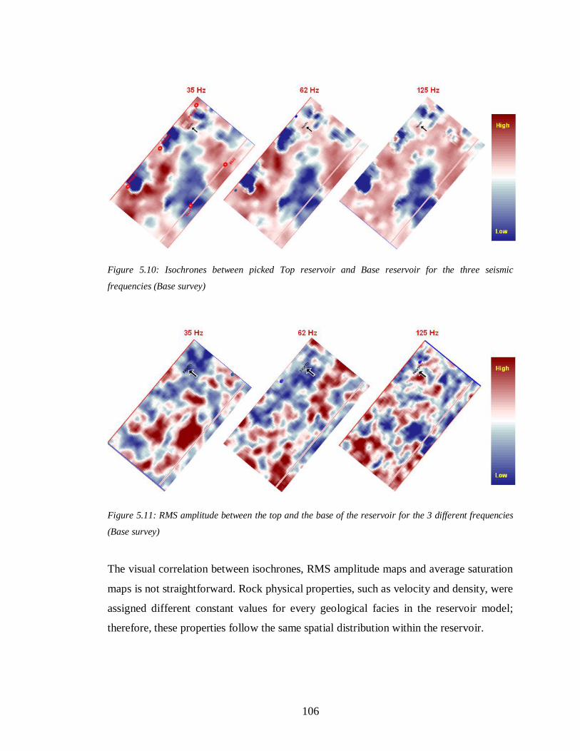
106

Figure 5.10: Isochrones between picked Top reservoir and Base reservoir for the three seismic

frequencies (Base survey)

Figure 5.11: RMS amplitude between the top and the base of the reservoir for the 3 different frequencies

(Base survey)

The visual correlation between isochrones, RMS amplitude maps and average saturation

maps is not straightforward. Rock physical properties, such as velocity and density, were

assigned different constant values for every geological facies in the reservoir model;

therefore, these properties follow the same spatial distribution within the reservoir.

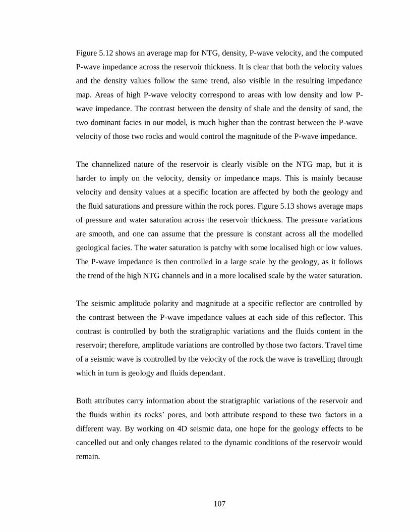
107

Figure 5.12 shows an average map for NTG, density, P-wave velocity, and the computed

P-wave impedance across the reservoir thickness. It is clear that both the velocity values

and the density values follow the same trend, also visible in the resulting impedance

map. Areas of high P-wave velocity correspond to areas with low density and low P-

wave impedance. The contrast between the density of shale and the density of sand, the

two dominant facies in our model, is much higher than the contrast between the P-wave

velocity of those two rocks and would control the magnitude of the P-wave impedance.

The channelized nature of the reservoir is clearly visible on the NTG map, but it is

harder to imply on the velocity, density or impedance maps. This is mainly because

velocity and density values at a specific location are affected by both the geology and

the fluid saturations and pressure within the rock pores. Figure 5.13 shows average maps

of pressure and water saturation across the reservoir thickness. The pressure variations

are smooth, and one can assume that the pressure is constant across all the modelled

geological facies. The water saturation is patchy with some localised high or low values.

The P-wave impedance is then controlled in a large scale by the geology, as it follows

the trend of the high NTG channels and in a more localised scale by the water saturation.

The seismic amplitude polarity and magnitude at a specific reflector are controlled by

the contrast between the P-wave impedance values at each side of this reflector. This

contrast is controlled by both the stratigraphic variations and the fluids content in the

reservoir; therefore, amplitude variations are controlled by those two factors. Travel time

of a seismic wave is controlled by the velocity of the rock the wave is travelling through

which in turn is geology and fluids dependant.

Both attributes carry information about the stratigraphic variations of the reservoir and

the fluids within its rocks’ pores, and both attribute respond to these two factors in a

different way. By working on 4D seismic data, one hope for the geology effects to be

cancelled out and only changes related to the dynamic conditions of the reservoir would

remain.

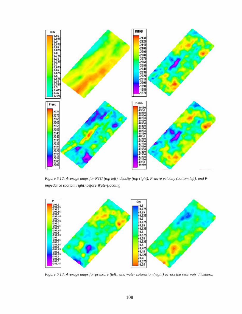
108

Figure 5.12: Average maps for NTG (top left), density (top right), P-wave velocity (bottom left), and P-

impedance (bottom right) before Waterflooding

Figure 5.13: Average maps for pressure (left), and water saturation (right) across the reservoir thickness.

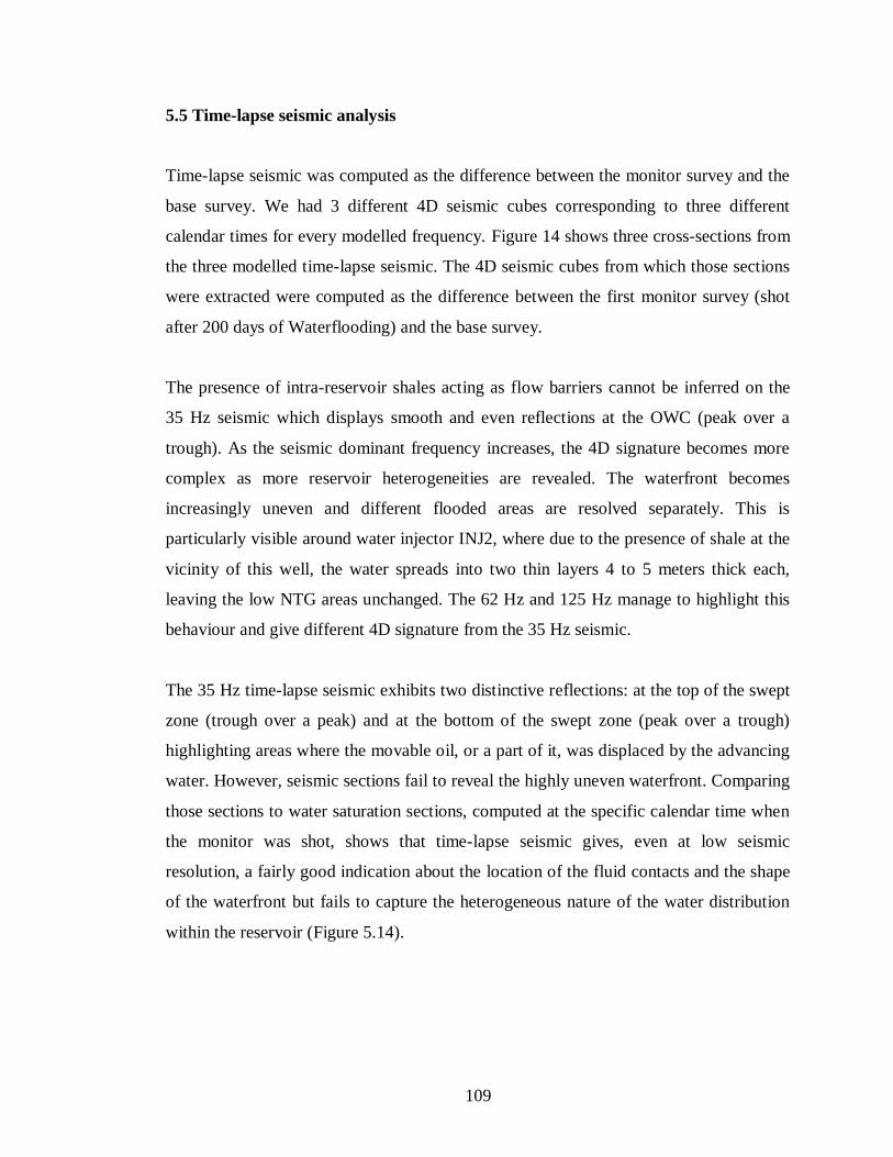
109

5.5 Time-lapse seismic analysis

Time-lapse seismic was computed as the difference between the monitor survey and the

base survey. We had 3 different 4D seismic cubes corresponding to three different

calendar times for every modelled frequency. Figure 14 shows three cross-sections from

the three modelled time-lapse seismic. The 4D seismic cubes from which those sections

were extracted were computed as the difference between the first monitor survey (shot

after 200 days of Waterflooding) and the base survey.

The presence of intra-reservoir shales acting as flow barriers cannot be inferred on the

35 Hz seismic which displays smooth and even reflections at the OWC (peak over a

trough). As the seismic dominant frequency increases, the 4D signature becomes more

complex as more reservoir heterogeneities are revealed. The waterfront becomes

increasingly uneven and different flooded areas are resolved separately. This is

particularly visible around water injector INJ2, where due to the presence of shale at the

vicinity of this well, the water spreads into two thin layers 4 to 5 meters thick each,

leaving the low NTG areas unchanged. The 62 Hz and 125 Hz manage to highlight this

behaviour and give different 4D signature from the 35 Hz seismic.

The 35 Hz time-lapse seismic exhibits two distinctive reflections: at the top of the swept

zone (trough over a peak) and at the bottom of the swept zone (peak over a trough)

highlighting areas where the movable oil, or a part of it, was displaced by the advancing

water. However, seismic sections fail to reveal the highly uneven waterfront. Comparing

those sections to water saturation sections, computed at the specific calendar time when

the monitor was shot, shows that time-lapse seismic gives, even at low seismic

resolution, a fairly good indication about the location of the fluid contacts and the shape

of the waterfront but fails to capture the heterogeneous nature of the water distribution

within the reservoir (Figure 5.14).

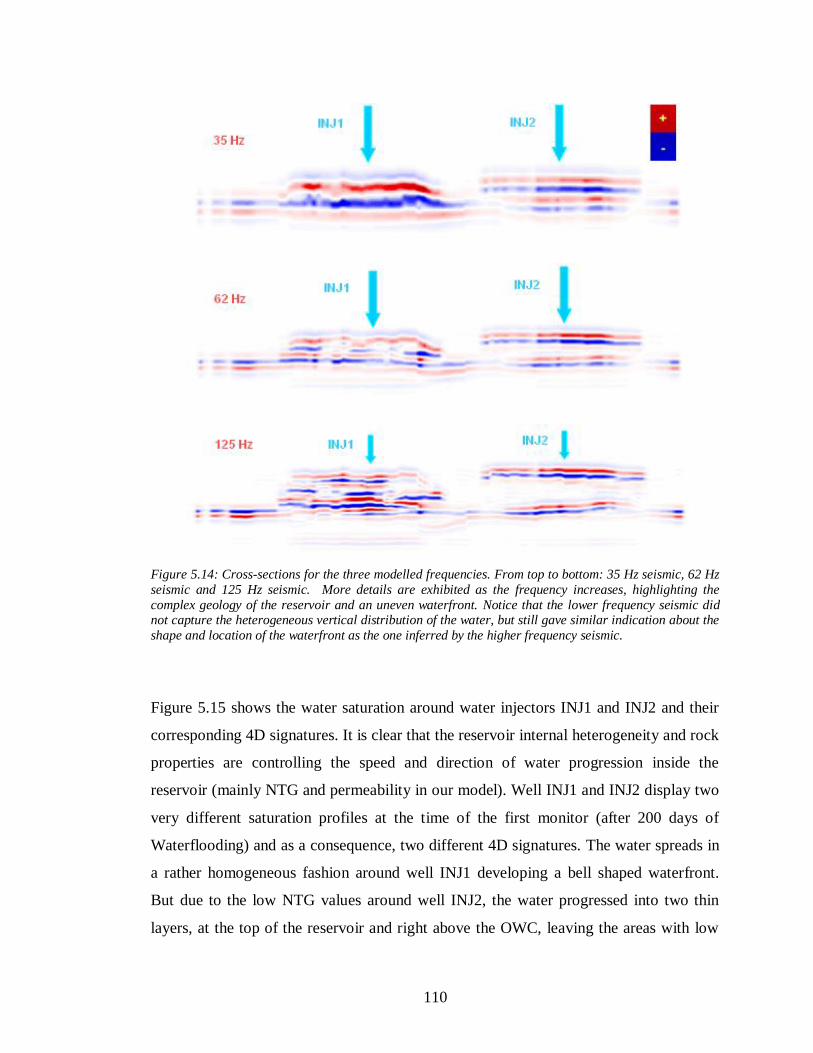
110

Figure 5.14: Cross-sections for the three modelled frequencies. From top to bottom: 35 Hz seismic, 62 Hz

seismic and 125 Hz seismic. More details are exhibited as the frequency increases, highlighting the

complex geology of the reservoir and an uneven waterfront. Notice that the lower frequency seismic did not capture the heterogeneous vertical distribution of the water, but still gave similar indication about the

shape and location of the waterfront as the one inferred by the higher frequency seismic.

Figure 5.15 shows the water saturation around water injectors INJ1 and INJ2 and their

corresponding 4D signatures. It is clear that the reservoir internal heterogeneity and rock

properties are controlling the speed and direction of water progression inside the

reservoir (mainly NTG and permeability in our model). Well INJ1 and INJ2 display two

very different saturation profiles at the time of the first monitor (after 200 days of

Waterflooding) and as a consequence, two different 4D signatures. The water spreads in

a rather homogeneous fashion around well INJ1 developing a bell shaped waterfront.

But due to the low NTG values around well INJ2, the water progressed into two thin

layers, at the top of the reservoir and right above the OWC, leaving the areas with low

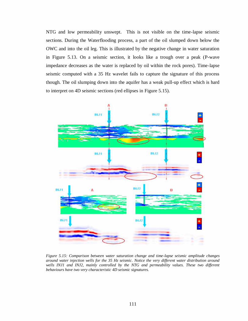
111

NTG and low permeability unswept. This is not visible on the time-lapse seismic

sections. During the Waterflooding process, a part of the oil slumped down below the

OWC and into the oil leg. This is illustrated by the negative change in water saturation

in Figure 5.13. On a seismic section, it looks like a trough over a peak (P-wave

impedance decreases as the water is replaced by oil within the rock pores). Time-lapse

seismic computed with a 35 Hz wavelet fails to capture the signature of this process

though. The oil slumping down into the aquifer has a weak pull-up effect which is hard

to interpret on 4D seismic sections (red ellipses in Figure 5.15).

Figure 5.15: Comparison between water saturation change and time-lapse seismic amplitude changes

around water injection wells for the 35 Hz seismic. Notice the very different water distribution around wells INJ1 and INJ2, mainly controlled by the NTG and permeability values. These two different

behaviours have two very characteristic 4D seismic signatures.

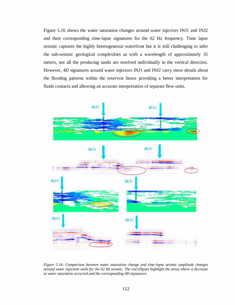
112

Figure 5.16 shows the water saturation changes around water injectors INJ1 and INJ2

and their corresponding time-lapse signatures for the 62 Hz frequency. Time lapse

seismic captures the highly heterogeneous waterfront but it is still challenging to infer

the sub-seismic geological complexities as with a wavelength of approximately 35

meters, not all the producing sands are resolved individually in the vertical direction.

However, 4D signatures around water injectors INJ1 and INJ2 carry more details about

the flooding patterns within the reservoir hence providing a better interpretation for

fluids contacts and allowing an accurate interpretation of separate flow units.


around water injection wells for the 62 Hz seismic. The red ellipses highlight the areas where a decrease

in water saturation occurred and the corresponding 4D signatures.

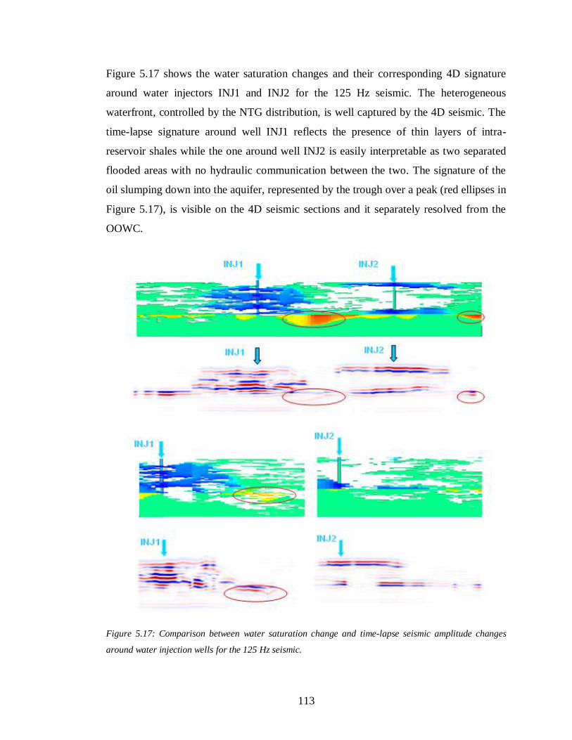
113

Figure 5.17 shows the water saturation changes and their corresponding 4D signature

around water injectors INJ1 and INJ2 for the 125 Hz seismic. The heterogeneous

waterfront, controlled by the NTG distribution, is well captured by the 4D seismic. The

time-lapse signature around well INJ1 reflects the presence of thin layers of intra-

reservoir shales while the one around well INJ2 is easily interpretable as two separated

flooded areas with no hydraulic communication between the two. The signature of the

oil slumping down into the aquifer, represented by the trough over a peak (red ellipses in

Figure 5.17), is visible on the 4D seismic sections and it separately resolved from the

OOWC.


around water injection wells for the 125 Hz seismic.

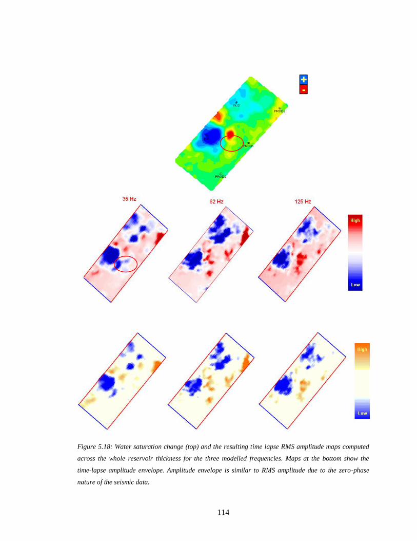
114

Figure 5.18: Water saturation change (top) and the resulting time lapse RMS amplitude maps computed

across the whole reservoir thickness for the three modelled frequencies. Maps at the bottom show the

time-lapse amplitude envelope. Amplitude envelope is similar to RMS amplitude due to the zero-phase

nature of the seismic data.

115

Figure 5.18 shows maps of the average water saturation change inside the reservoir after

200 days of Waterflooding along with the resulting time-lapse RMS amplitude and

amplitude envelope maps for the three modelled frequencies. At this early stage of

Waterflooding, the water had not reached the producing wells yet. The saturation

difference map (top) shows strong water saturation increase around injection well INJ1,

and to a lesser extend around injection well INJ2. This is understood to be a direct result

of the averaging process. In fact, even though the saturation changes around the two

wells are of similar magnitude in the active cells (sand) around the two injectors; the low

NTG cells, set to be inactive in our simulation model and are present in a greater number

around well INJ2, had their properties unchanged by the injection of water yielding an

average change of a weaker magnitude around INJ2. Had we opted to compute the

average saturation change only across the sand cells, we would have had an average map

exhibiting the same magnitude in water saturation change around both wells. We chose

to compute the average maps across the whole reservoir in order for them to be

comparable to the average 4D amplitude RMS maps computed from 4D seismic cubes.

The 4D amplitude RMS maps exhibit amplitude dimming resulting from impedance

increases caused by water encroachment. Sustained high amplitudes and low

impedances are areas that have remaining hydrocarbons present (bypassed oil) while

areas with no amplitude change are areas unswept by the advancing water. The maps

computed from the three different seismic sets, corresponding to the three different

dominant frequencies, all exhibit areas with a decrease in amplitude around water

injectors, an increase in amplitude where the oil replaced water in the aquifer, and very

weak to nil signal elsewhere. It is on the level of details and the accurate mapping of

fluids contacts that they differ.

The 35 Hz seismic gave a fairly good indication of the swept areas inside the reservoir.

However, it was less accurate in areas with low NTG values due to the averaging

properties of seismic waves propagation. Interpretation of the 4D signature of

Waterflooding around both injection wells without a prior knowledge of the reservoir

internal geology could lead to an erroneous assessment of the reservoir heterogeneities

116

and compartmentalisation. The signature around well INJ1 displays features that could

be easily interpreted as flooded areas where no saturation change has occurred in the

simulation model (red ellipse in Figure 5.18). It also shows a dimming in 4D seismic

amplitude where we had a negative change in water saturation (red ellipse in Figure

5.18), contrarily to what is expected. The 4D seismic signature around INJ2 could be

interpreted as the result of flow barriers within the reservoir at the vicinity of this well as

it is divided into two separate features inferring that there is no hydraulic communication

between the corresponding areas within the reservoir, which is not correct. This is

further highlighted in the amplitude envelope map. As the dominant seismic frequency

increases, the seismic resolution increases as a consequence and more subtle details

about the swept areas are shown in the 4D RMS amplitude maps. Most importantly, the

62 Hz seismic and the 125 Hz seismic successfully produced continuous drainage maps

similar to those computed from the fluids flow simulation. Interpretation of 4D RMS

amplitude and 4D RMS amplitude envelope maps yield an accurate mapping of fluids

contacts and the highly uneven fluid front. The 125 Hz seismic resolved flooded areas as

small as a few meter large. It also shows a less smooth and continuous waterfront,

highlighting the strong variations of rock properties inside the reservoir.

As the Waterflooding process continued, water spread further into the reservoir

producing an increasingly complex 4D signature. Figure 5.19 shows cross-sections of

the 4D seismic created for the three studied frequencies along with the corresponding

water saturation change profile. More reservoir internal heterogeneities are revealed

showing that repeated 4D seismic acquisitions can be of a great value in managing

Waterflooding in complex reservoirs and also in building a solid understanding of the

reservoir geological settings. The accurate interpretation of the 4D signature requires

such an understanding. Figure 5.20 shows an average map of water saturation changes

across the reservoir and the corresponding RMS amplitude and RMS amplitude

envelope for the three studied frequencies.

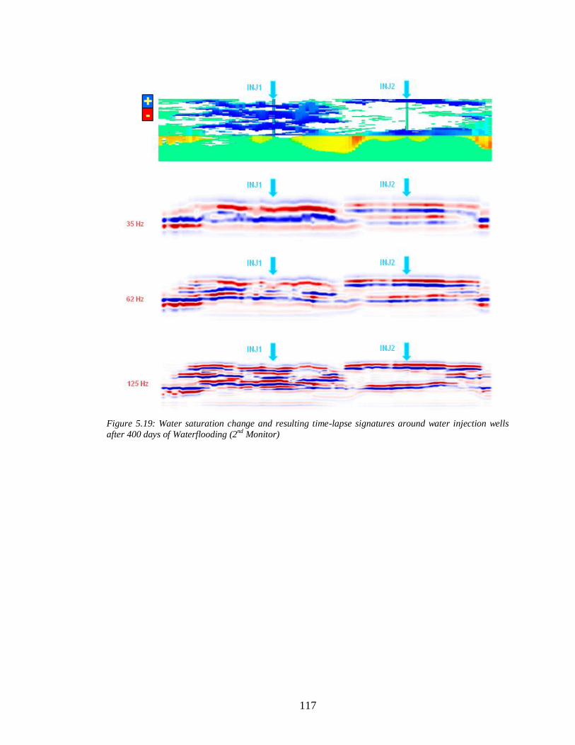
117

Figure 5.19: Water saturation change and resulting time-lapse signatures around water injection wells

after 400 days of Waterflooding (2nd Monitor)

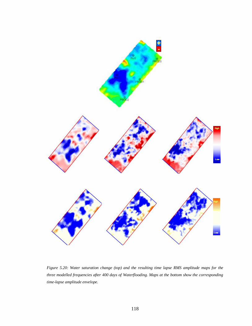
118

Figure 5.20: Water saturation change (top) and the resulting time lapse RMS amplitude maps for the

three modelled frequencies after 400 days of Waterflooding. Maps at the bottom show the corresponding

time-lapse amplitude envelope.

119

5.6 Conclusion

The results of the Waterflooding simulation, performed on the Ainsa II reservoir model,

were inserted into a petro-physical model to compute the reservoir rock seismic

properties at different calendar times. P-wave velocity, S-wave velocity, and density

cubes corresponding to different stages of Waterflooding were generated. An increase in

P-wave impedance of up to 7% could be expected as a direct result of water substituting

oil within the rocks’ pores. Saturation changes have a dominant effect on the time-lapse

signature of Waterflooding, while the pressure had a global dimming effect on the

magnitude of changes observed on time-lapse seismic attributes, due mainly to the

absence of any internal compartmentalisation within the reservoir. The pressure drop

caused similar changes in the rocks’ seismic properties at either side of the waterfront.

Synthetic seismic created using three different frequencies imaged the reservoir’s

interior in different ways. As the seismic dominant frequency increased from 35 Hz to

125 Hz, the seismic vertical resolution increased and different interferences patterns

occurs. On 3D seismic sections, different channels within the reservoir were resolved

separately on the high resolution seismic. Tuning phenomenon is observed for the three

modelled frequencies due to the presence of very thin beds (1-2 meter thick). The

interpretation of the OOWC or the MOWC on those sections is challenging because the

reflections at the fluids front are obscured by reflections from geological interfaces. The

complex geology of the reservoir resulted in 3 different RMS seismic amplitude maps

showing an increasing degree of heterogeneities as the seismic dominant frequency

increased. The fluids-front is hard to interpret on both RMS seismic amplitude maps and

isochrones maps as those two attributes carry information about the reservoir geology

and fluids but are affected by them in different ways.

The analysis of time-lapse seismic sections and attributes maps showed that once the

―geology effect‖ is removed, the three modelled seismic sets, with increasing dominant

frequency, had similar signatures of the Waterflooding process. The shape and location

120

of the waterfront can be interpreted on both low and high frequency seismic, with

increasing level of details as the seismic frequency increases.

121

Chapter 6

Time-lapse seismic attributes analysis in a deepwater stacked turbidite

reservoir

Time lapse seismic attributes analysis is performed on a high resolution seismic created

from the simulation outputs of Waterflooding in the synthetic turbidite reservoir. Both

time shift attributes and 4D amplitude RMS attributes are studied. The combined

response from these two attributes is used to better assess the efficiency of the

Waterflooding process by identifying swept areas and fluids contact more accurately.

122

6.1 Introduction

The success of time lapse monitoring of Waterflooding in geologically complex

environments depends on several factors. The quality of seismic data plays a major

factor toward a successful time lapse interpretation of the fluid front and the drainage

patterns inside the reservoir. Careful planning for acquisition and processing of time

lapse seismic data is of paramount importance as it increases the repeatability and

decreases seismic noise. There were several major advances in time lapse seismic

processing leading to excellent data quality with high repeatability and excellent signal

to noise ratio. These advances, coupled with increasingly high seismic resolution, led to

a better imaging of complex turbidite reservoirs and a more detailed understanding of

their internal geology and production mechanisms.

The improvement of 4D seismic data quality led to more ambitious application of the

technique; which evolved from qualitative observations to becoming more quantitative.

Dynamic reservoir changes, such as pressure and fluids saturation, were directly

estimated from 4D seismic data and used to update flow simulation models. Time-lapse

seismic data was used successfully in the assessing of reservoir connectivity and in

computing permeability trends and faults transmissibility. Time-lapse seismic data

proved to be a very valuable part of Waterflooding monitoring programs. It allows the

accurate mapping of fluids contacts movement and the identification of unswept areas

thus bringing more confidence into any proposed infill drilling location and providing

the possibility of pro-active actions to be taken in order to optimise reservoir

performance.

We performed an in-depth analysis of the 4D seismic signature of Waterflooding in The

Ainsa II reservoir model. The study is carried out on the synthetic seismic data created

with a Ricker wavelet with a 62 Hz peak frequency. Seismic data with a peak frequency

of 62 Hz is considered to be high resolution seismic data in the oil industry. Figure 6.1

shows a comparison between the synthetic seismic created using a 62 Hz Ricker wavelet

and the synthetic seismic created using a wavelet extracted from the high resolution

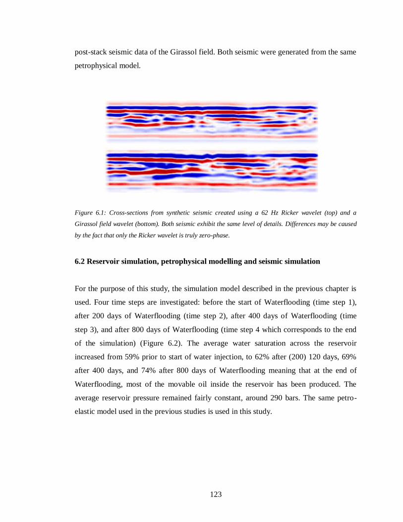
123

post-stack seismic data of the Girassol field. Both seismic were generated from the same

petrophysical model.

Figure 6.1: Cross-sections from synthetic seismic created using a 62 Hz Ricker wavelet (top) and a

Girassol field wavelet (bottom). Both seismic exhibit the same level of details. Differences may be caused

by the fact that only the Ricker wavelet is truly zero-phase.

6.2 Reservoir simulation, petrophysical modelling and seismic simulation

For the purpose of this study, the simulation model described in the previous chapter is

used. Four time steps are investigated: before the start of Waterflooding (time step 1),

after 200 days of Waterflooding (time step 2), after 400 days of Waterflooding (time

step 3), and after 800 days of Waterflooding (time step 4 which corresponds to the end

of the simulation) (Figure 6.2). The average water saturation across the reservoir

increased from 59% prior to start of water injection, to 62% after (200) 120 days, 69%

after 400 days, and 74% after 800 days of Waterflooding meaning that at the end of

Waterflooding, most of the movable oil inside the reservoir has been produced. The

average reservoir pressure remained fairly constant, around 290 bars. The same petro-

elastic model used in the previous studies is used in this study.

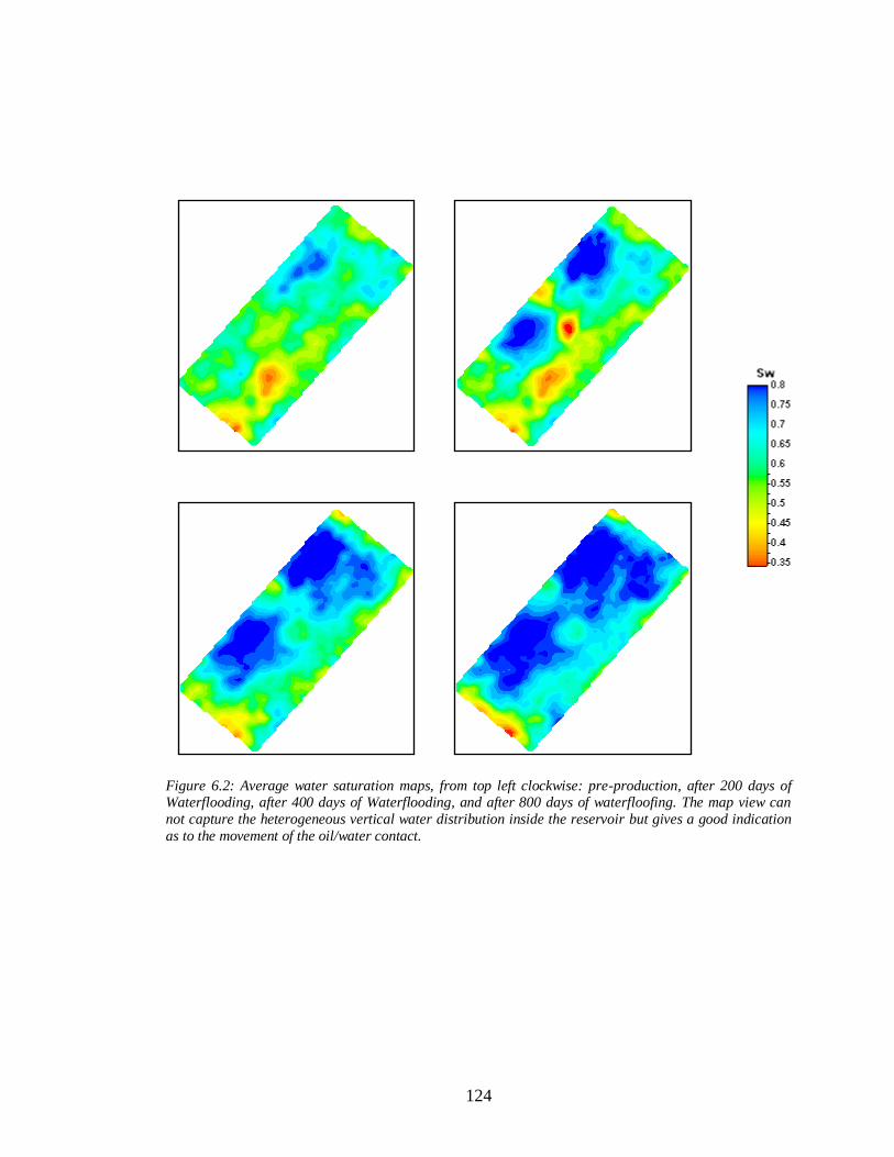
124

Figure 6.2: Average water saturation maps, from top left clockwise: pre-production, after 200 days of Waterflooding, after 400 days of Waterflooding, and after 800 days of waterfloofing. The map view can

not capture the heterogeneous vertical water distribution inside the reservoir but gives a good indication

as to the movement of the oil/water contact.

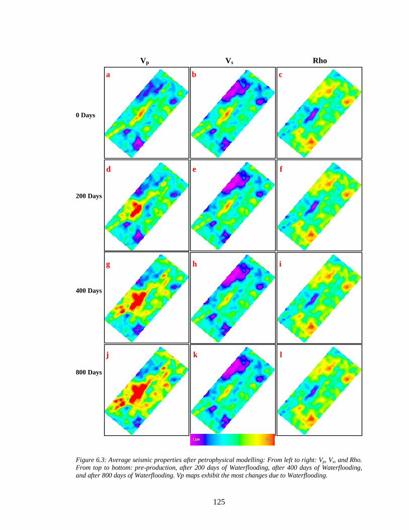
125

Vp Vs Rho

a b c

0 Days

d e f

200 Days

g h i

400 Days

j k l

800 Days

Figure 6.3: Average seismic properties after petrophysical modelling: From left to right: Vp, Vs, and Rho.

From top to bottom: pre-production, after 200 days of Waterflooding, after 400 days of Waterflooding,

and after 800 days of Waterflooding. Vp maps exhibit the most changes due to Waterflooding.

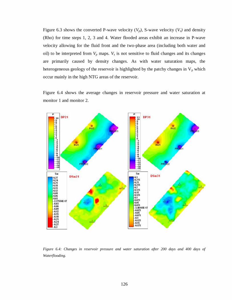
126

Figure 6.3 shows the converted P-wave velocity (Vp), S-wave velocity (Vs) and density

(Rho) for time steps 1, 2, 3 and 4. Water flooded areas exhibit an increase in P-wave

velocity allowing for the fluid front and the two-phase area (including both water and

oil) to be interpreted from Vp maps. Vs is not sensitive to fluid changes and its changes

are primarily caused by density changes. As with water saturation maps, the

heterogeneous geology of the reservoir is highlighted by the patchy changes in Vp which

occur mainly in the high NTG areas of the reservoir.

Figure 6.4 shows the average changes in reservoir pressure and water saturation at

monitor 1 and monitor 2.

Figure 6.4: Changes in reservoir pressure and water saturation after 200 days and 400 days of

Waterflooding.

127

Prior to Waterflooding, the reservoir pressure was constant across the reservoir. At the

start of the Waterflooding process, pressure changes were localised at the well locations.

A pressure increase of up to 11 bar (160 psi) is observed at the water injection wells

while a pressure decrease of up to 15 bar (218 psi) is observed at the producing wells.

As the Waterflooding proceeds, a smooth pressure front progresses from the injection

flank (over-pressurised area) to the producing flank of the reservoir (under-pressurised

area) unconditional of the underlying reservoir geology. The water injection/production

scenario was set so the pressure gradient created at the start of the Waterflooding

process remains constant until the end of the Waterflooding.

The water saturation changes were patchy and heterogeneous and are highly correlated

to the high permeability/high NTG zones of the reservoir. Both negative and positive

changes in water saturation were observed. At the start of the Waterflooding, the

waterfront advanced from the injectors displacing the oil in an almost piston like manner

toward the producers. A part of the injected water slumped down below the OOWC and

got trapped there. As the Waterflooding continued, a part of this trapped water is

recovered, but some of it remained trapped there until the end of the Waterflooding

process.

Figure 6.5 shows average changes in P-wave velocity, S-wave velocity and density at

the two monitors. Warm colours represent an increase in the displayed property after

Waterflooding, while cool colours represent a decrease. The similarity in the patterns

between the P-wave velocity difference map and the water saturation difference map

infers that the mechanisms responsible for velocity changes at the two monitors are

highly conditioned by the water saturation changes. The substitution of oil with water

within the rocks’ pores resulted in an increase of the P-wave velocity by up to 35 ms-1

,

while a maximum of 23 ms-1

decrease is observed where water substituted oil. Changes

in S-wave velocity are smoother and present similar patterns than changes in pressure.

But since S-wave velocity is affected by changes in density, which in turn is affected by

both changes in pressure and fluids saturation, some visual correlations between Vs

changes and water saturation changes are obvious.

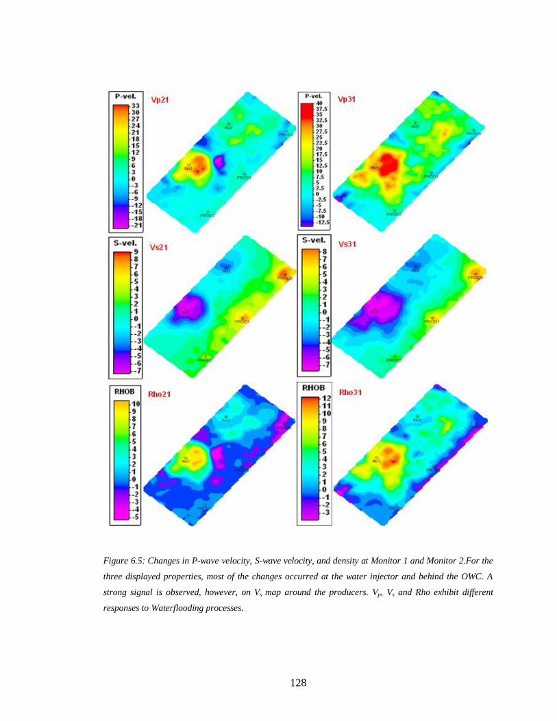
128

Figure 6.5: Changes in P-wave velocity, S-wave velocity, and density at Monitor 1 and Monitor 2.For the

three displayed properties, most of the changes occurred at the water injector and behind the OWC. A

strong signal is observed, however, on Vs map around the producers. Vp, Vs and Rho exhibit different

responses to Waterflooding processes.

129

Figure 6.6 shows cross-plots of P-wave velocity changes against average water

saturation changes, at the time of the first and the second monitor. A linear relationship

links changes in Vp and changes in Sw. At the time of the first monitor, water saturation

increased by only 3%, as the water didn’t reach far into the reservoir. Only few cells

were water flooded, and water saturation changes were significant only at the vicinity of

the injection wells. This can be seen in the cross-plot graphs, where (Figure 6.6.a) most

of the data was grouped in a cluster extending across water saturation changes ranging

from -0.1 to 0.1. As the Waterflooding proceeded, a larger part of the reservoir was

water flooded and the range of water saturation changes widened resulting in the cluster

of data being less dense. The pressure has little impact on the P-wave velocity changes

but it can be seen on the cross-plot graphs that areas where the pressure decreased would

see a bigger change in Vp than areas where the pressure remained constant or increased.

Figure 6.7 shows a cross-plot of changes in Vp as a function of pressure changes. It is

clear that changes in Vp are not related to pressure changes.

Figure 6.8 shows cross-plots of changes in S-wave velocity as a function of changes in

pressure at Monitor 1 and Monitor 2. Changes in Vs are controlled by changes in

reservoir pressure in a linear fashion. The cross-plots for Monitor 1 and Monitor 2 data

look similar, suggesting that even though changes in Vs are mainly controlled by the

pressure evolution inside the reservoir, these changes happened early in the

Waterflooding process and stabilised after that. Examination of the evolution of S-wave

velocity as a function of reservoir pressure changes over time, in a Waterflooding

process, can give valuable information as to reservoir compartmentalisation and

hydraulic communication.

Indeed, areas where significant changes in S-wave velocity, in a Waterflooding process,

can be interpreted as a hydraulically isolated compartment inside the reservoir. If these

changes are observed near a fault, they could give indication as to the sealing nature of

that fault.

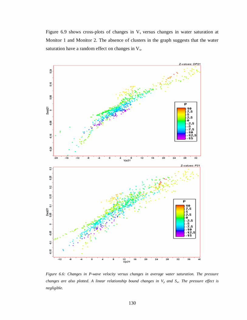
130

Figure 6.9 shows cross-plots of changes in Vs versus changes in water saturation at

Monitor 1 and Monitor 2. The absence of clusters in the graph suggests that the water

saturation have a random effect on changes in Vs.

Figure 6.6: Changes in P-wave velocity versus changes in average water saturation. The pressure

changes are also plotted. A linear relationship bound changes in Vp and Sw. The pressure effect is

negligible.

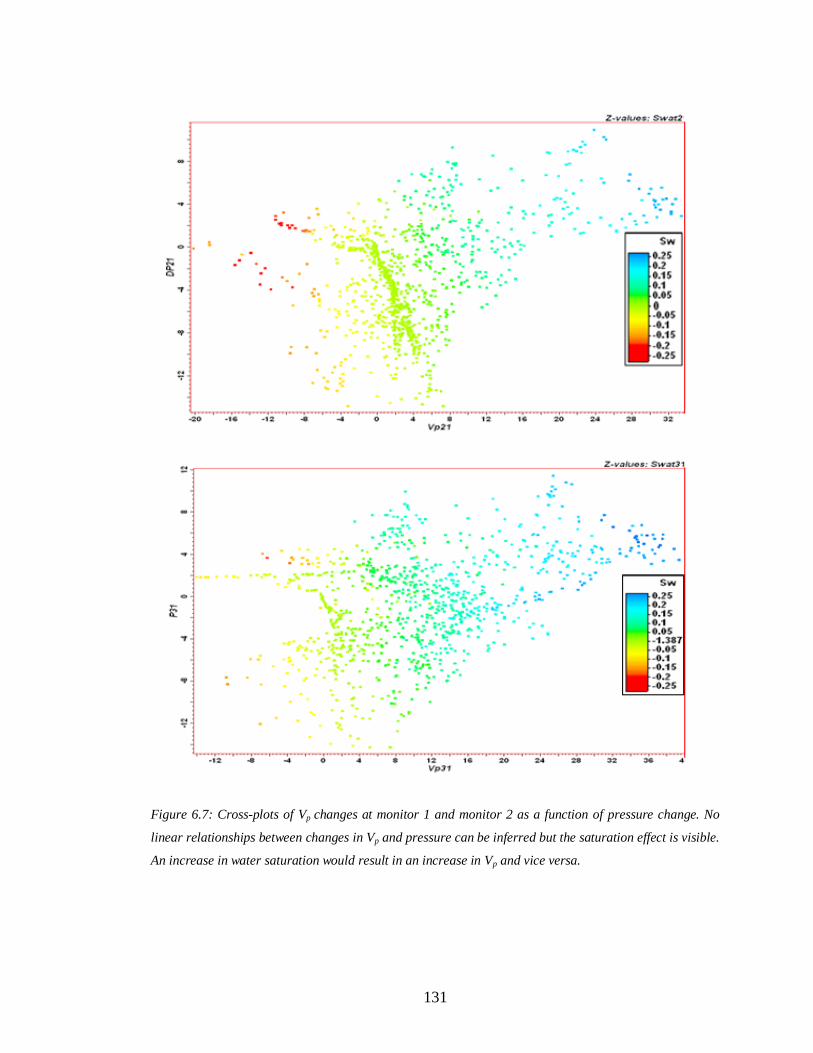
131

Figure 6.7: Cross-plots of Vp changes at monitor 1 and monitor 2 as a function of pressure change. No

linear relationships between changes in Vp and pressure can be inferred but the saturation effect is visible.

An increase in water saturation would result in an increase in Vp and vice versa.

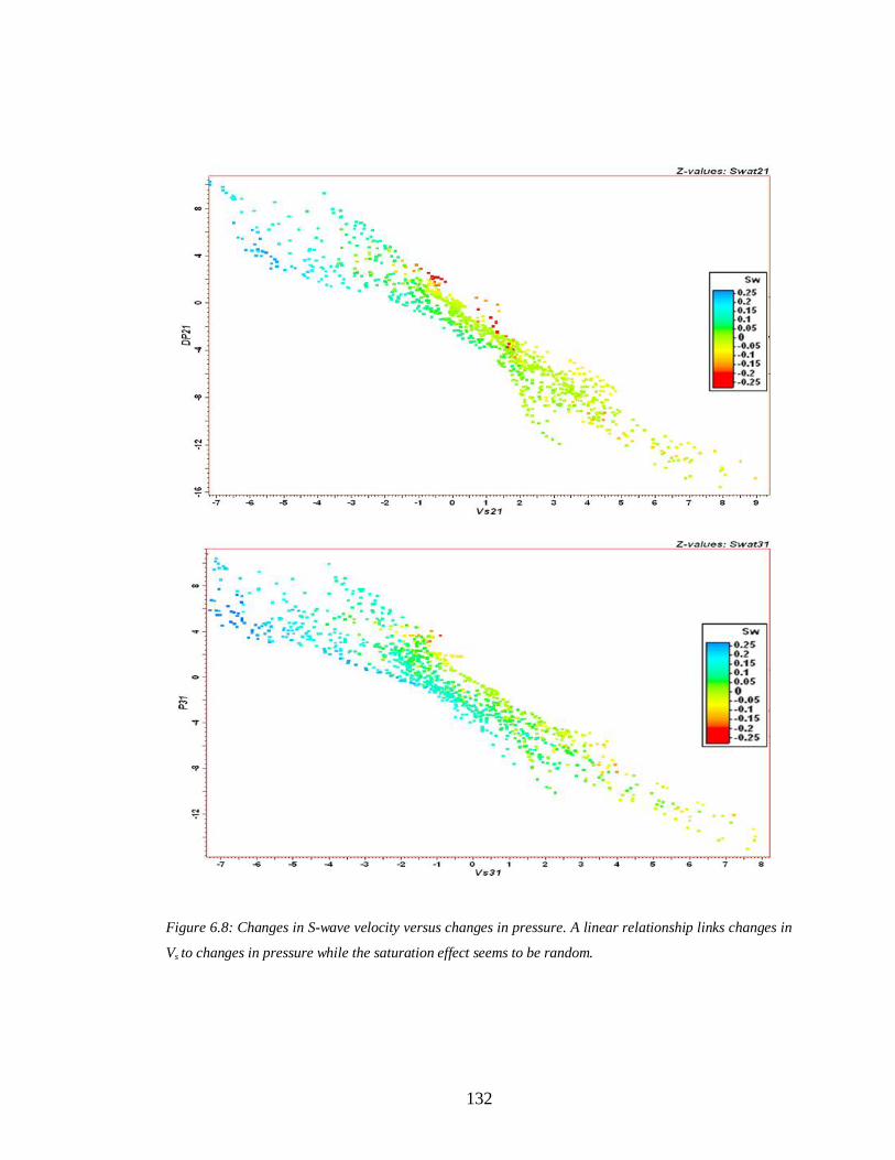
132

Figure 6.8: Changes in S-wave velocity versus changes in pressure. A linear relationship links changes in

Vs to changes in pressure while the saturation effect seems to be random.

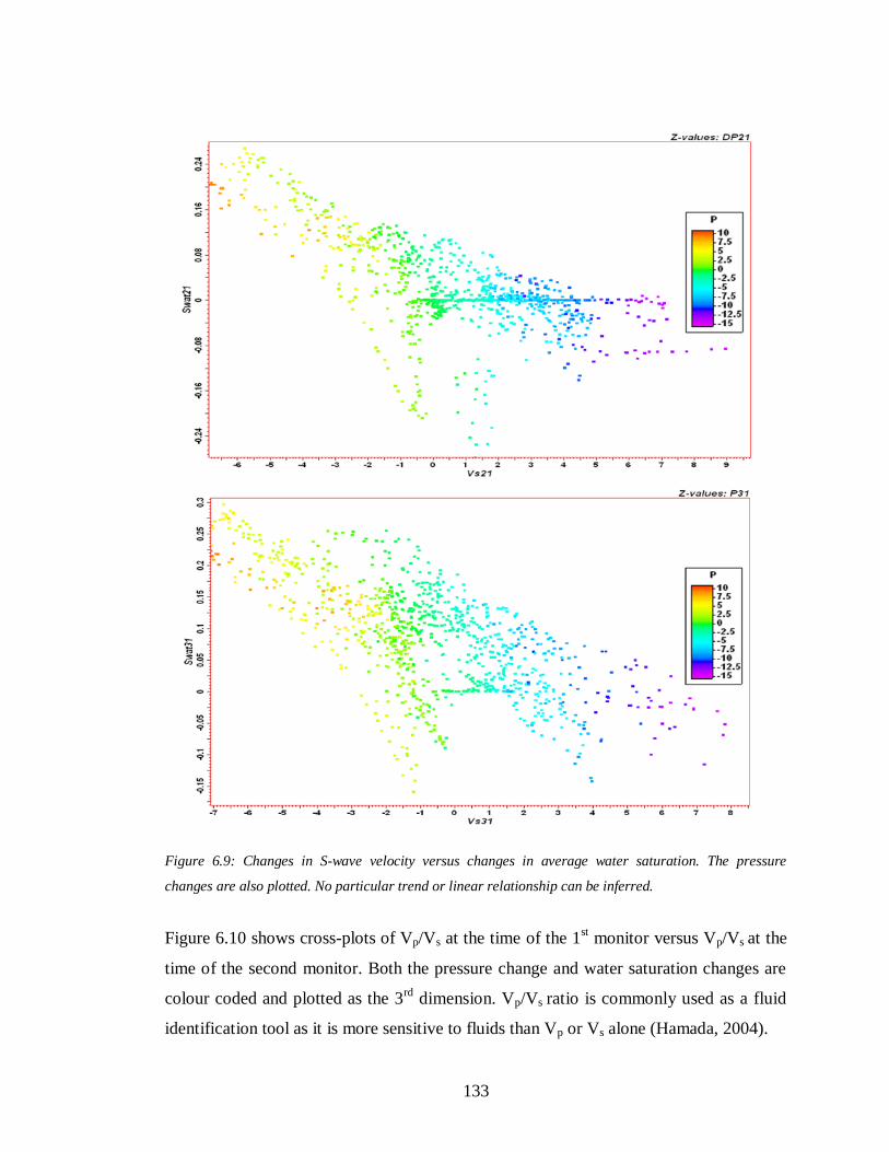
133

Figure 6.9: Changes in S-wave velocity versus changes in average water saturation. The pressure

changes are also plotted. No particular trend or linear relationship can be inferred.

Figure 6.10 shows cross-plots of Vp/Vs at the time of the 1st monitor versus Vp/Vs at the

time of the second monitor. Both the pressure change and water saturation changes are

colour coded and plotted as the 3rd

dimension. Vp/Vs ratio is commonly used as a fluid

identification tool as it is more sensitive to fluids than Vp or Vs alone (Hamada, 2004).

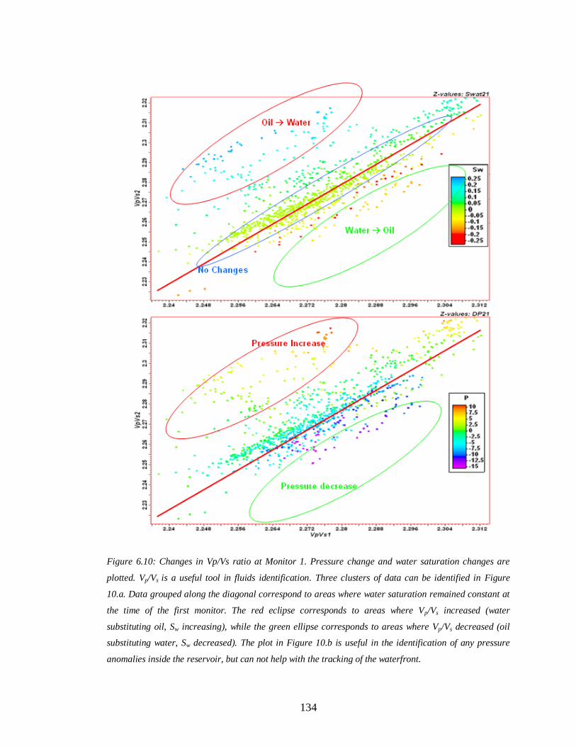
134

Figure 6.10: Changes in Vp/Vs ratio at Monitor 1. Pressure change and water saturation changes are

plotted. Vp/Vs is a useful tool in fluids identification. Three clusters of data can be identified in Figure

10.a. Data grouped along the diagonal correspond to areas where water saturation remained constant at

the time of the first monitor. The red eclipse corresponds to areas where Vp/Vs increased (water

substituting oil, Sw increasing), while the green ellipse corresponds to areas where Vp/Vs decreased (oil

substituting water, Sw decreased). The plot in Figure 10.b is useful in the identification of any pressure

anomalies inside the reservoir, but can not help with the tracking of the waterfront.

135

Time-lapse seismic was computed as the difference between the monitor surveys and the

base survey. The difference between the monitor survey and the base survey is a seismic

cube (4D seismic cube) where geology effects (assumed to be constant during the fluids

flow simulation and the seismic modelling) are cancelled, leaving only the effects of

pressure change and fluids saturation changes. The pressure has a global dimming effect

on seismic attributes which would not be investigated in this study as the pressure

fluctuations were kept to a minimum during simulation. Four synthetic seismic cubes,

corresponding to four different stages of the Waterflooding process, were created and

used in this study. The first 4D seismic cube would highlight the changes in fluids

distribution inside the reservoir after 200 days of water injection (1st Monitor – Base),

the second after 400 days (2nd

Monitor – Base), and the third at the end of Waterflooding

(3rd

Monitor – Base).

6.3 Time-lapse seismic analyses

The turbidite reservoir model used for the purpose of this study is highly heterogeneous

in the geological sense. The reservoir heterogeneity is captured in our model through

stratigraphic variations in net-to-gross and the occurrence of intra-reservoir shales. This

heterogeneity, present on a variety of scales within the reservoir, will strongly influence

both vertical and lateral connectivity and hence fluid flow behaviour during production

or injection (MacBeth et al., 2005). It could compromise our quantitative understanding

of the time-lapse seismic signature. Figure 6.11 presents one-dimensional schematics

illustrating the influence of the OWC movement in a clean sandstone reservoir and in a

heterogeneous turbidite reservoir. The impedance values for the turbidite case were

derived from impedance logs extracted from the petrophysical model at production well

Prod2. The light blue colour represents the impedance change due to water replacing oil

within the reservoir rocks. The water sand is modelled to be completely water saturated

(aquifer, in blue in Figure 6.11), while the oil sand contains connate water saturation,

Swc.

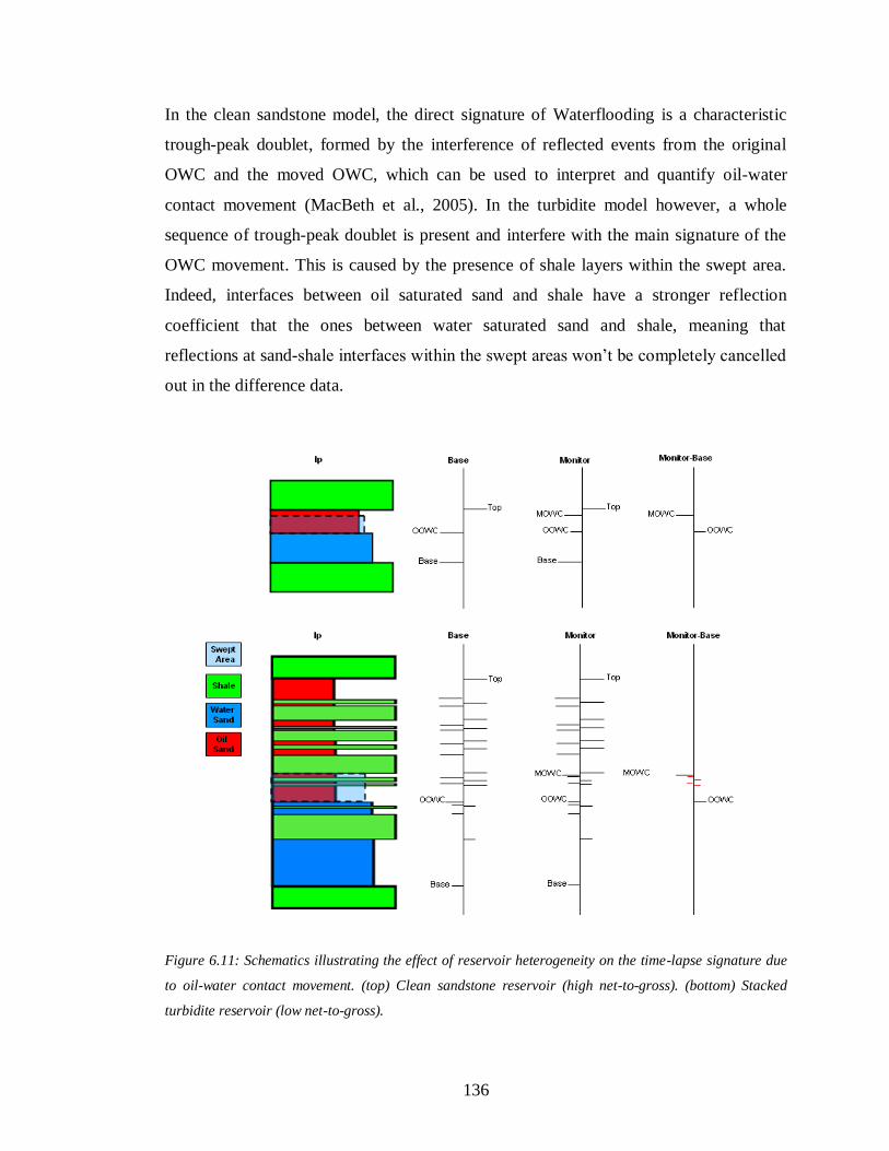
136

In the clean sandstone model, the direct signature of Waterflooding is a characteristic

trough-peak doublet, formed by the interference of reflected events from the original

OWC and the moved OWC, which can be used to interpret and quantify oil-water

contact movement (MacBeth et al., 2005). In the turbidite model however, a whole

sequence of trough-peak doublet is present and interfere with the main signature of the

OWC movement. This is caused by the presence of shale layers within the swept area.

Indeed, interfaces between oil saturated sand and shale have a stronger reflection

coefficient that the ones between water saturated sand and shale, meaning that

reflections at sand-shale interfaces within the swept areas won’t be completely cancelled

out in the difference data.

Figure 6.11: Schematics illustrating the effect of reservoir heterogeneity on the time-lapse signature due

to oil-water contact movement. (top) Clean sandstone reservoir (high net-to-gross). (bottom) Stacked

turbidite reservoir (low net-to-gross).

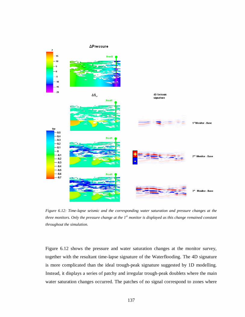
137

Figure 6.12: Time-lapse seismic and the corresponding water saturation and pressure changes at the

three monitors. Only the pressure change at the 1st monitor is displayed as this change remained constant

throughout the simulation.

Figure 6.12 shows the pressure and water saturation changes at the monitor survey,

together with the resultant time-lapse signature of the Waterflooding. The 4D signature

is more complicated than the ideal trough-peak signature suggested by 1D modelling.

Instead, it displays a series of patchy and irregular trough-peak doublets where the main

water saturation changes occurred. The patches of no signal correspond to zones where

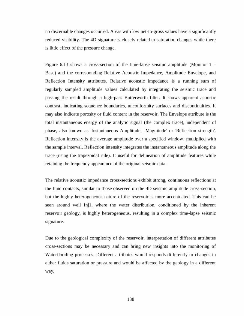
138

no discernable changes occurred. Areas with low net-to-gross values have a significantly

reduced visibility. The 4D signature is closely related to saturation changes while there

is little effect of the pressure change.

Figure 6.13 shows a cross-section of the time-lapse seismic amplitude (Monitor 1 –

Base) and the corresponding Relative Acoustic Impedance, Amplitude Envelope, and

Reflection Intensity attributes. Relative acoustic impedance is a running sum of

regularly sampled amplitude values calculated by integrating the seismic trace and

passing the result through a high-pass Butterworth filter. It shows apparent acoustic

contrast, indicating sequence boundaries, unconformity surfaces and discontinuities. It

may also indicate porosity or fluid content in the reservoir. The Envelope attribute is the

total instantaneous energy of the analytic signal (the complex trace), independent of

phase, also known as 'Instantaneous Amplitude', 'Magnitude' or 'Reflection strength'.

Reflection intensity is the average amplitude over a specified window, multiplied with

the sample interval. Reflection intensity integrates the instantaneous amplitude along the

trace (using the trapezoidal rule). It useful for delineation of amplitude features while

retaining the frequency appearance of the original seismic data.

The relative acoustic impedance cross-sections exhibit strong, continuous reflections at

the fluid contacts, similar to those observed on the 4D seismic amplitude cross-section,

but the highly heterogeneous nature of the reservoir is more accentuated. This can be

seen around well Inj1, where the water distribution, conditioned by the inherent

reservoir geology, is highly heterogeneous, resulting in a complex time-lapse seismic

signature.

Due to the geological complexity of the reservoir, interpretation of different attributes

cross-sections may be necessary and can bring new insights into the monitoring of

Waterflooding processes. Different attributes would responds differently to changes in

either fluids saturation or pressure and would be affected by the geology in a different

way.

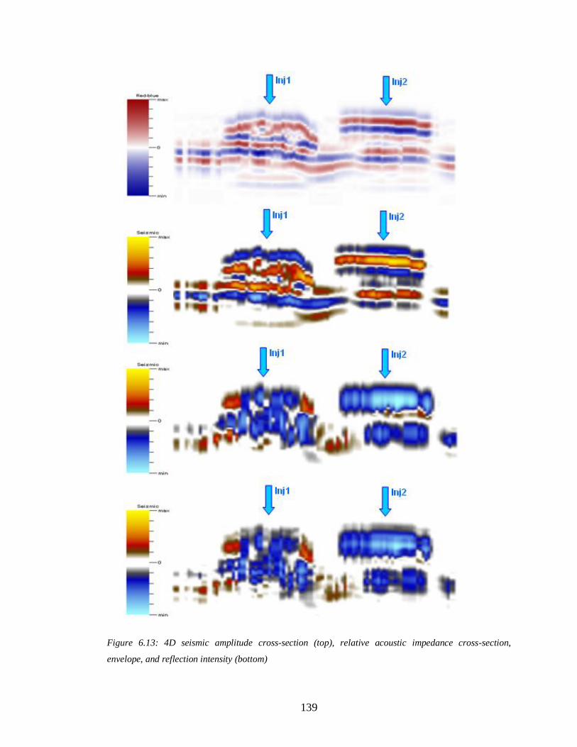
139

Figure 6.13: 4D seismic amplitude cross-section (top), relative acoustic impedance cross-section,

envelope, and reflection intensity (bottom)

140

6.3.1 Time-shift analysis

Reservoir thickness-time was computed as the difference between the travel time at the

top reservoir horizon and the travel time at the base reservoir horizon. The average

reservoir thickness in time is 43 ms. As water is injected into the reservoir; the drained

areas will see their rock velocities increasing allowing seismic waves to propagate faster

through the reservoir thus decreasing travel time. Figure 6.14 shows the computed

isochrones for the different studied time-steps.

The average reservoir thickness-time decreased through time from 43.7 ms before the

start of Waterflooding, to 43.3 at the end of the process (after 800 days). As water is

injected into the reservoir, computed isochrones exhibit more heterogeneity highlighting

a patchy water distribution associated with complex drainage patterns guided by the

reservoir inherent geology.

Interpretation of time-shifts observed on the simple sand block model (chapter 3)

suggests that time shift computed across the whole reservoir thickness at a specific

location is proportional to the height of the swept area at that location. While this

statement holds true in a simple sand block model, it is not straightforward to extend it

to geologically complex reservoirs. The heterogeneities of reservoir rock properties (i.e.

NTG, permeability, porosity, etc) and the presence of intra-reservoir shales acting as

flow barriers would condition the distribution of the injected water within the reservoir.

To accurately correlate the observed time-shift with water saturation changes, one must

account for the reservoir geology.

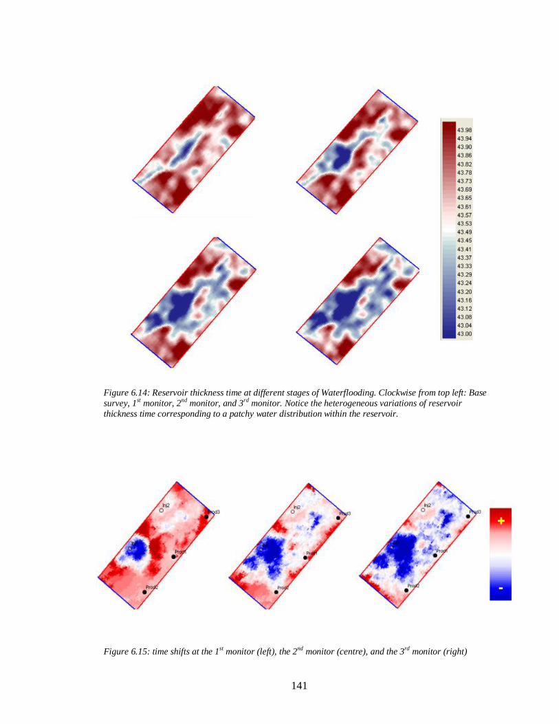
141

Figure 6.14: Reservoir thickness time at different stages of Waterflooding. Clockwise from top left: Base

survey, 1st monitor, 2nd monitor, and 3rd monitor. Notice the heterogeneous variations of reservoir

thickness time corresponding to a patchy water distribution within the reservoir.

Figure 6.15: time shifts at the 1st monitor (left), the 2nd monitor (centre), and the 3rd monitor (right)

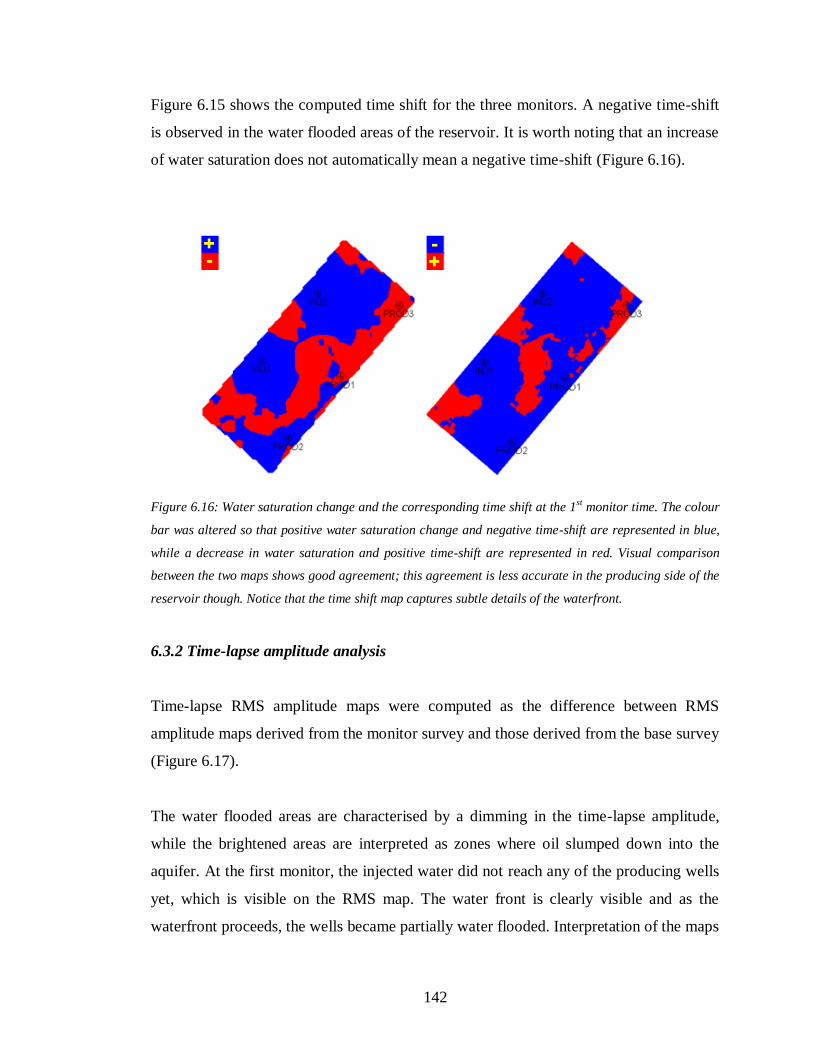
142

Figure 6.15 shows the computed time shift for the three monitors. A negative time-shift

is observed in the water flooded areas of the reservoir. It is worth noting that an increase

of water saturation does not automatically mean a negative time-shift (Figure 6.16).

Figure 6.16: Water saturation change and the corresponding time shift at the 1st monitor time. The colour

bar was altered so that positive water saturation change and negative time-shift are represented in blue,

while a decrease in water saturation and positive time-shift are represented in red. Visual comparison

between the two maps shows good agreement; this agreement is less accurate in the producing side of the

reservoir though. Notice that the time shift map captures subtle details of the waterfront.

6.3.2 Time-lapse amplitude analysis

Time-lapse RMS amplitude maps were computed as the difference between RMS

amplitude maps derived from the monitor survey and those derived from the base survey

(Figure 6.17).

The water flooded areas are characterised by a dimming in the time-lapse amplitude,

while the brightened areas are interpreted as zones where oil slumped down into the

aquifer. At the first monitor, the injected water did not reach any of the producing wells

yet, which is visible on the RMS map. The water front is clearly visible and as the

waterfront proceeds, the wells became partially water flooded. Interpretation of the maps

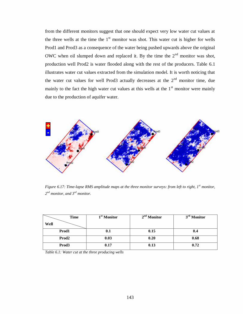
143

from the different monitors suggest that one should expect very low water cut values at

the three wells at the time the 1st monitor was shot. This water cut is higher for wells

Prod1 and Prod3 as a consequence of the water being pushed upwards above the original

OWC when oil slumped down and replaced it. By the time the 2nd

monitor was shot,

production well Prod2 is water flooded along with the rest of the producers. Table 6.1

illustrates water cut values extracted from the simulation model. It is worth noticing that

the water cut values for well Prod3 actually decreases at the 2nd

monitor time, due

mainly to the fact the high water cut values at this wells at the 1st monitor were mainly

due to the production of aquifer water.

Figure 6.17: Time-lapse RMS amplitude maps at the three monitor surveys: from left to right, 1st monitor,

2nd monitor, and 3rd monitor.

Time

Well

1st Monitor 2

nd Monitor 3

rd Monitor

Prod1 0.1 0.15 0.4

Prod2 0.03 0.20 0.68

Prod3 0.17 0.13 0.72

Table 6.1: Water cut at the three producing wells

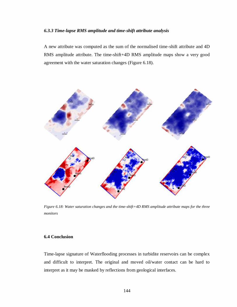
144

6.3.3 Time-lapse RMS amplitude and time-shift attribute analysis

A new attribute was computed as the sum of the normalised time-shift attribute and 4D

RMS amplitude attribute. The time-shift+4D RMS amplitude maps show a very good

agreement with the water saturation changes (Figure 6.18).

Figure 6.18: Water saturation changes and the time-shift+4D RMS amplitude attribute maps for the three

monitors

6.4 Conclusion

Time-lapse signature of Waterflooding processes in turbidite reservoirs can be complex

and difficult to interpret. The original and moved oil/water contact can be hard to

interpret as it may be masked by reflections from geological interfaces.

145

Analysis of P-wave and S-wave velocity cubes showed that these two properties respond

in different ways to Waterflooding. Vp is sensitive to water saturation changes while Vs

is sensitive to pressure changes. Vp/Vs ratio can be used as a robust fluids indicator

provided that both the base seismic survey and the monitor seismic survey have the

correct velocity model. Petrophysical modelling suggests that P-wave velocity can be

extremely sensitive to water saturation changes. Even the smallest changes (less than

10%) would have a noticeable effect on Vp values, which is of crucial importance when

time-lapse seismic is to be used in a quantitative way.

Interpretation of time-lapse seismic cross-sections is challenging and the inclusion of

different attributes in the interpretation workflow might be necessary in order to assess

the complexity of the Waterflooding signature.

Interpretation of time-lapse attribute maps, computed of an RMS average across the

reservoir thickness is useful in the global assessment Waterflooding efficiency as they

provide a fair indication as to fluids fronts and bypassed oil. But the extrapolation to the

vertical dimension may be very challenging in turbidite reservoirs.

146

Chapter 7

Conclusions and recommendations for future research

In this thesis, Waterflooding processes in geologically complex reservoirs were

investigated. The investigation followed three different, yet inter-related directions:

reservoir modelling and fluid flow simulation, petrophysical modelling, and seismic

modelling and interpretation. This chapter presents a summary of the results from each

chapter and the main concluding remarks of the thesis.

Recommendations for further improvement and application of this work are also

addressed.

147

7.1 Conclusions

Several lessons have been learnt from the application of this approach to the different

synthetic data cases:

1- Time-lapse seismic is used in a qualitative, semi-quantitative, and quantitative way

to monitor Waterflooding processes. For the Time-lapse seismic data to be used in a

quantitative way, calibration with other data (production data, etc) is needed.

2- Analytical and numerical engineering techniques were developed to assess the

efficiency of Waterflooding processes. At present, numerical simulation models

have assumed a considerable lead in Waterflooding efficiency calculations and

become the standard tool for such studies. Numerical simulation of Waterflooding

processes require the building of a numerical reservoir model, where the reservoir is

subdivided into blocks or cells in each of which are reservoir rocks properties and

quantities of fluids subject to the laws of fluid mechanics. Their essential advantage

is to be able to represent the variations in characteristics of the reservoir, the fluids,

the flow rates to the wells and the pressure within the reservoir. Analytical methods

aim at generating a relationship between fractional flow and oil recovery. The

reservoir is assumed to be zero dimensional and displays a tank like behaviour. The

Buckley-Leverett equation is used to describe fluid flow inside the reservoir by

determining an expression for the velocity of a plane of constant water saturation

passing through the reservoir. A practical application of the equation is through the

use of the Welge equation. To account for reservoirs heterogeneities, the reservoir is

divided into several layers and recovery efficiency calculations are performed for

each layer. The analytical methods tend to over simplify the reservoir geology by

not including areal heterogeneities and lateral variations of layers thickness.

3- Permeability and its degree of variation across the reservoir is the most important

parameter controlling the displacement efficiency in the case of water injection.

148

4- The 4D seismic signature of Waterflooding processes is a combination of pressure,

saturation, and temperature changes within the reservoir at the monitor time,

assuming the reservoir is not geomechanically active. The substitution of oil by

water increases the P-wave velocity of the rock, while an increase in pore pressure

decreases the P-wave velocity of the rock. During Waterflooding, saturation

changes arrive after the pressure changes resulting in three distinct zones inside the

reservoir that would exhibit different responses to Waterflooding (Figure 7.1):

Behind the waterfront: The water saturation and the pore pressure increase ,so

Vp can theoretically either increase or decrease. In all of our petrophysical

modelling studies, Vp increased by up to 9%, regardless of the reservoir setting

or production scenario. This is due to the fact that the saturation effect is

stronger than the pressure effect.

Between the Water Front and the Pressure Front: Water saturation unchanged,

while the pore pressure increases so Vp is unchanged or decreases.

Beyond the Pressure Front: The water saturation is unchanged, the pore

pressure is unchanged or decreases, so Vp increase. This phenomenon was not

observed in any of our petrophysical simulation studies, as the reservoir

pressure equilibrated shortly (few days) after the start of water injection. In real

case studies, this behaviour can be observed as a pressure build-up effect in the

vicinity of sealing faults and at the boundaries of non-communication reservoir

compartments.

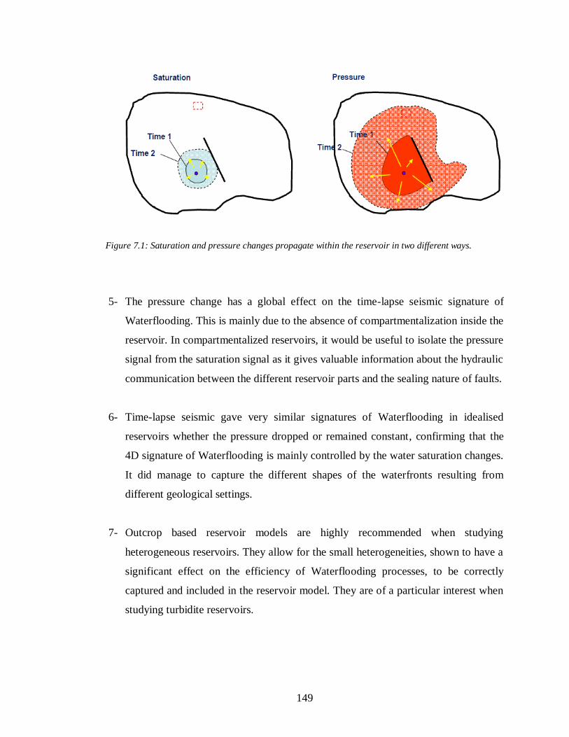
149

Figure 7.1: Saturation and pressure changes propagate within the reservoir in two different ways.

5- The pressure change has a global effect on the time-lapse seismic signature of

Waterflooding. This is mainly due to the absence of compartmentalization inside the

reservoir. In compartmentalized reservoirs, it would be useful to isolate the pressure

signal from the saturation signal as it gives valuable information about the hydraulic

communication between the different reservoir parts and the sealing nature of faults.

6- Time-lapse seismic gave very similar signatures of Waterflooding in idealised

reservoirs whether the pressure dropped or remained constant, confirming that the

4D signature of Waterflooding is mainly controlled by the water saturation changes.

It did manage to capture the different shapes of the waterfronts resulting from

different geological settings.

7- Outcrop based reservoir models are highly recommended when studying

heterogeneous reservoirs. They allow for the small heterogeneities, shown to have a

significant effect on the efficiency of Waterflooding processes, to be correctly

captured and included in the reservoir model. They are of a particular interest when

studying turbidite reservoirs.

150

8- The same reservoir architecture picked up from the outcrop analogue can produce

very different seismic response from one reservoir to another due to their different

rock properties, misleading the interpretation of the reservoir when high density

well control is not available. Accurate properties modelling will highly benefit the

understanding of the seismic signature, especially in deep and ultra-deep reservoirs

reducing the economic risks. When the seismic modelling is aimed at understanding

the time-lapse seismic signature of Waterflooding in a given reservoir, one should

construct an accurate database of rock parameters and fluids properties for that very

same reservoir.

9- RMS seismic attributes maps are commonly used in time-lapse seismic

interpretation. RMS averages are a good statistical measure of the magnitude of a

seismic trace. Comparing RMS seismic attributes maps to average maps of reservoir

properties (pressure, saturation, NTG, etc) should be performed with great care.

Tuning phenomenon should also be considered.

7.2 Recommendations for future work

The investigation presented in this thesis have been developed and applied on synthetic

data. Synthetic reservoir models, regardless of how realistic they can be, are merely a

simplified representation of the characteristics of the subsurface. Based on lessons

learned from this study, further research is needed to refine and make this approach

more robust when applied to synthetic data and ultimately real data. This further

research could be addressed under the following categories:

7.2.1 Building the simulation model

Virtually every turbidite reservoir contains significant amounts of shale. Shales either

divide the reservoirs into separate hydraulic units, or, if they are discontinuous, set a

tortuous environment in which fluids flow occurs. Although the sand/shale sequence in

the well vicinity may be known, a reliable reservoir description must define

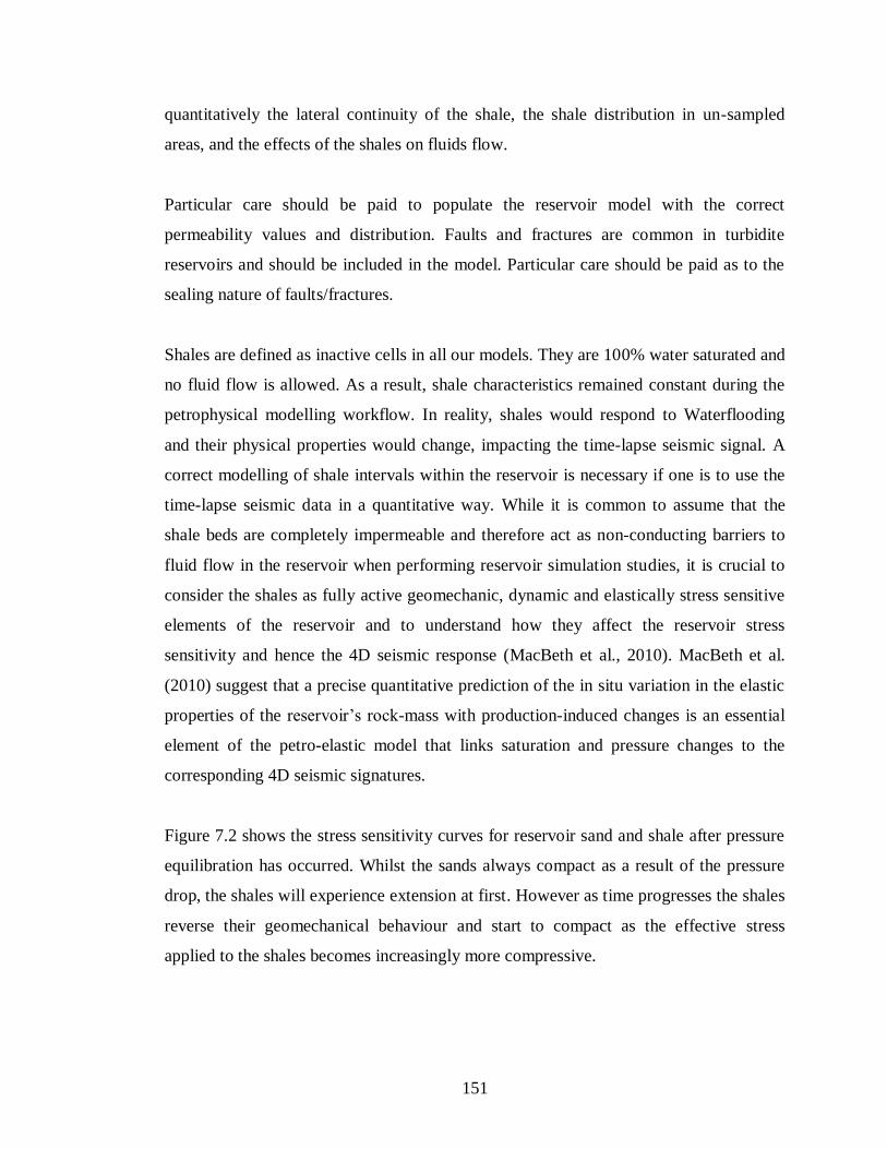
http://en.wikipedia.org/wiki/Statistics

http://en.wikipedia.org/wiki/Magnitude_(mathematics)

151

quantitatively the lateral continuity of the shale, the shale distribution in un-sampled

areas, and the effects of the shales on fluids flow.

Particular care should be paid to populate the reservoir model with the correct

permeability values and distribution. Faults and fractures are common in turbidite

reservoirs and should be included in the model. Particular care should be paid as to the

sealing nature of faults/fractures.

Shales are defined as inactive cells in all our models. They are 100% water saturated and

no fluid flow is allowed. As a result, shale characteristics remained constant during the

petrophysical modelling workflow. In reality, shales would respond to Waterflooding

and their physical properties would change, impacting the time-lapse seismic signal. A

correct modelling of shale intervals within the reservoir is necessary if one is to use the

time-lapse seismic data in a quantitative way. While it is common to assume that the

shale beds are completely impermeable and therefore act as non-conducting barriers to

fluid flow in the reservoir when performing reservoir simulation studies, it is crucial to

consider the shales as fully active geomechanic, dynamic and elastically stress sensitive

elements of the reservoir and to understand how they affect the reservoir stress

sensitivity and hence the 4D seismic response (MacBeth et al., 2010). MacBeth et al.

(2010) suggest that a precise quantitative prediction of the in situ variation in the elastic

properties of the reservoir’s rock-mass with production-induced changes is an essential

element of the petro-elastic model that links saturation and pressure changes to the

corresponding 4D seismic signatures.

Figure 7.2 shows the stress sensitivity curves for reservoir sand and shale after pressure

equilibration has occurred. Whilst the sands always compact as a result of the pressure

drop, the shales will experience extension at first. However as time progresses the shales

reverse their geomechanical behaviour and start to compact as the effective stress

applied to the shales becomes increasingly more compressive.

152

Figure 7.2: sand and shale stress sensitivity curves. (after MacBeth et al., 2010)

7.2.2 Petro-elastic modelling

An accurate Petro-Elastic model is of paramount importance when performing forward

seismic modelling. To accurately replicate the observed time-lapse seismic signature of

a given reservoir, one must account for the overburden heterogeneities. Domes et al.

(2009) showed that errors originating from sand channels, faults or geomechanical

changes above the reservoir are supposed to impact the time-lapse data.

In our modelling workflow, the overburden and underburden were defined as a

homogeneous half-space, which is a flawed simplification of reality. In fact, the

overburden is a part of the sedimentary basin enclosing the reservoir and it features all

kind of heterogeneities common to sedimentary formations (Figure 7.3) (channels,

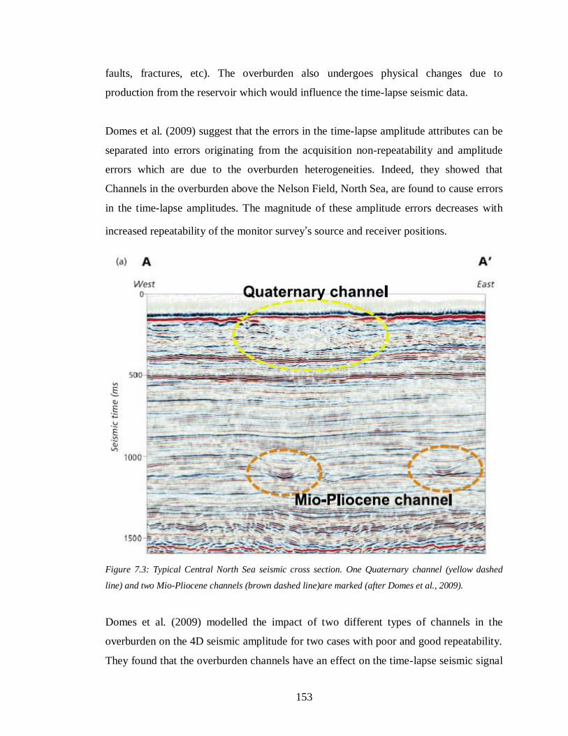
153

faults, fractures, etc). The overburden also undergoes physical changes due to

production from the reservoir which would influence the time-lapse seismic data.

Domes et al. (2009) suggest that the errors in the time-lapse amplitude attributes can be

separated into errors originating from the acquisition non-repeatability and amplitude

errors which are due to the overburden heterogeneities. Indeed, they showed that

Channels in the overburden above the Nelson Field, North Sea, are found to cause errors

in the time-lapse amplitudes. The magnitude of these amplitude errors decreases with

increased repeatability of the monitor survey’s source and receiver positions.

Figure 7.3: Typical Central North Sea seismic cross section. One Quaternary channel (yellow dashed

line) and two Mio-Pliocene channels (brown dashed line)are marked (after Domes et al., 2009).

Domes et al. (2009) modelled the impact of two different types of channels in the

overburden on the 4D seismic amplitude for two cases with poor and good repeatability.

They found that the overburden channels have an effect on the time-lapse seismic signal

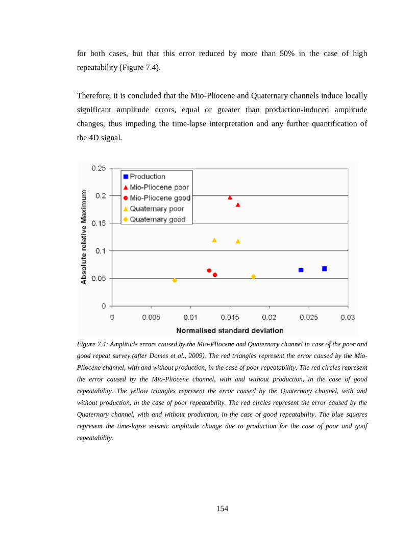
154

for both cases, but that this error reduced by more than 50% in the case of high

repeatability (Figure 7.4).

Therefore, it is concluded that the Mio-Pliocene and Quaternary channels induce locally

significant amplitude errors, equal or greater than production-induced amplitude

changes, thus impeding the time-lapse interpretation and any further quantification of

the 4D signal.

Figure 7.4: Amplitude errors caused by the Mio-Pliocene and Quaternary channel in case of the poor and

good repeat survey.(after Domes et al., 2009). The red triangles represent the error caused by the Mio-

Pliocene channel, with and without production, in the case of poor repeatability. The red circles represent

the error caused by the Mio-Pliocene channel, with and without production, in the case of good

repeatability. The yellow triangles represent the error caused by the Quaternary channel, with and

without production, in the case of poor repeatability. The red circles represent the error caused by the

Quaternary channel, with and without production, in the case of good repeatability. The blue squares

represent the time-lapse seismic amplitude change due to production for the case of poor and goof

repeatability.

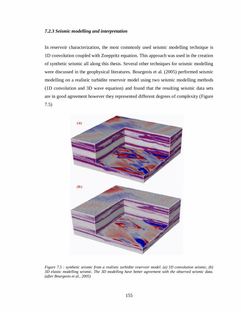
155

7.2.3 Seismic modelling and interpretation

In reservoir characterization, the most commonly used seismic modelling technique is

1D convolution coupled with Zoeppritz equation. This approach was used in the creation

of synthetic seismic all along this thesis. Several other techniques for seismic modelling

were discussed in the geophysical literatures. Bourgeois et al. (2005) performed seismic

modelling on a realistic turbidite reservoir model using two seismic modelling methods

(1D convolution and 3D wave equation) and found that the resulting seismic data sets

are in good agreement however they represented different degrees of complexity (Figure

7.5)

Figure 7.5 : synthetic seismic from a realistic turbidite reservoir model. (a) 1D convolution seismic, (b)

3D elastic modelling seismic. The 3D modelling have better agreement with the observed seismic data.

(after Bourgeois et al., 2005)

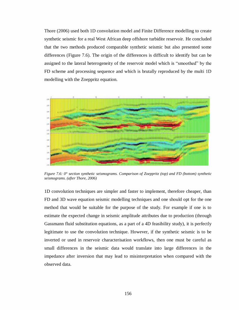
156

Thore (2006) used both 1D convolution model and Finite Difference modelling to create

synthetic seismic for a real West African deep offshore turbidite reservoir. He concluded

that the two methods produced comparable synthetic seismic but also presented some

differences (Figure 7.6). The origin of the differences is difficult to identify but can be

assigned to the lateral heterogeneity of the reservoir model which is ―smoothed‖ by the

FD scheme and processing sequence and which is brutally reproduced by the multi 1D

modelling with the Zoeppritz equation.

Figure 7.6: 0° section synthetic seismograms. Comparison of Zoeppritz (top) and FD (bottom) synthetic

seismograms. (after Thore, 2006)

1D convolution techniques are simpler and faster to implement, therefore cheaper, than

FD and 3D wave equation seismic modelling techniques and one should opt for the one

method that would be suitable for the purpose of the study. For example if one is to

estimate the expected change in seismic amplitude attributes due to production (through

Gassmann fluid substitution equations, as a part of a 4D feasibility study), it is perfectly

legitimate to use the convolution technique. However, if the synthetic seismic is to be

inverted or used in reservoir characterisation workflows, then one must be careful as

small differences in the seismic data would translate into large differences in the

impedance after inversion that may lead to misinterpretation when compared with the

observed data.

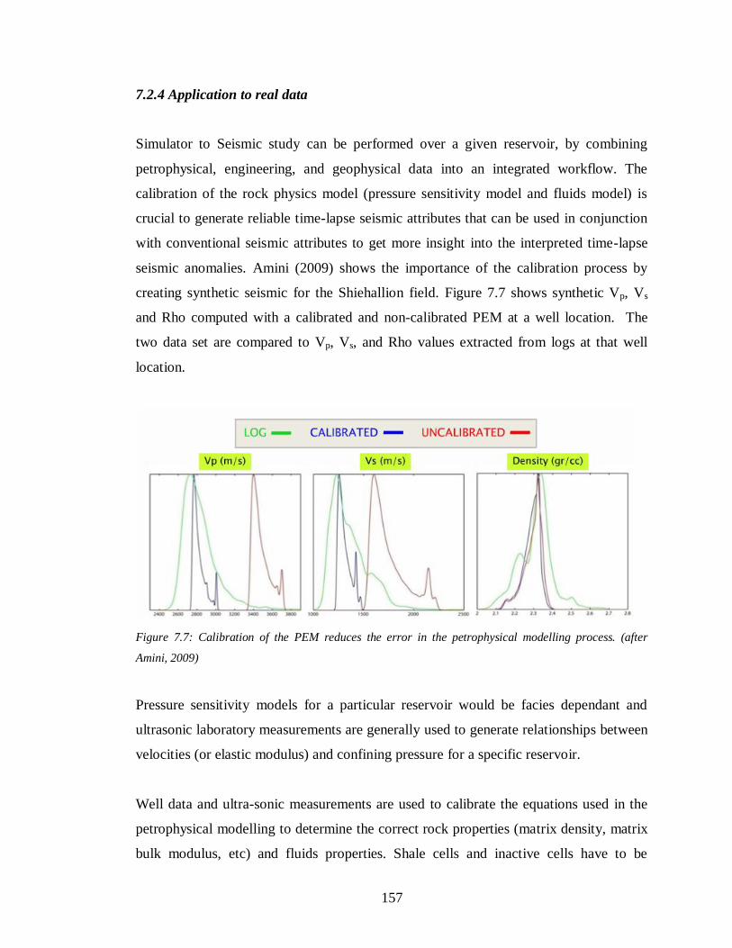
157

7.2.4 Application to real data

Simulator to Seismic study can be performed over a given reservoir, by combining

petrophysical, engineering, and geophysical data into an integrated workflow. The

calibration of the rock physics model (pressure sensitivity model and fluids model) is

crucial to generate reliable time-lapse seismic attributes that can be used in conjunction

with conventional seismic attributes to get more insight into the interpreted time-lapse

seismic anomalies. Amini (2009) shows the importance of the calibration process by

creating synthetic seismic for the Shiehallion field. Figure 7.7 shows synthetic Vp, Vs

and Rho computed with a calibrated and non-calibrated PEM at a well location. The

two data set are compared to Vp, Vs, and Rho values extracted from logs at that well

location.

Figure 7.7: Calibration of the PEM reduces the error in the petrophysical modelling process. (after

Amini, 2009)

Pressure sensitivity models for a particular reservoir would be facies dependant and

ultrasonic laboratory measurements are generally used to generate relationships between

velocities (or elastic modulus) and confining pressure for a specific reservoir.

Well data and ultra-sonic measurements are used to calibrate the equations used in the

petrophysical modelling to determine the correct rock properties (matrix density, matrix

bulk modulus, etc) and fluids properties. Shale cells and inactive cells have to be

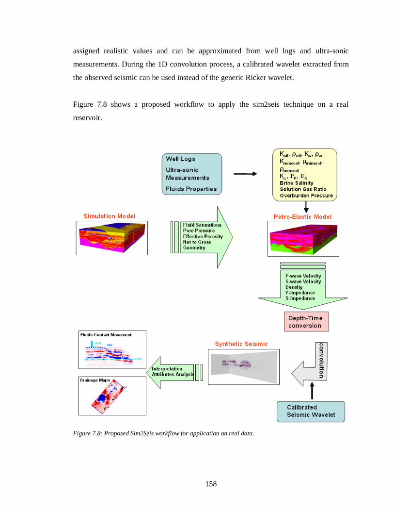
158

assigned realistic values and can be approximated from well logs and ultra-sonic

measurements. During the 1D convolution process, a calibrated wavelet extracted from

the observed seismic can be used instead of the generic Ricker wavelet.

Figure 7.8 shows a proposed workflow to apply the sim2seis technique on a real

reservoir.

Figure 7.8: Proposed Sim2Seis workflow for application on real data.

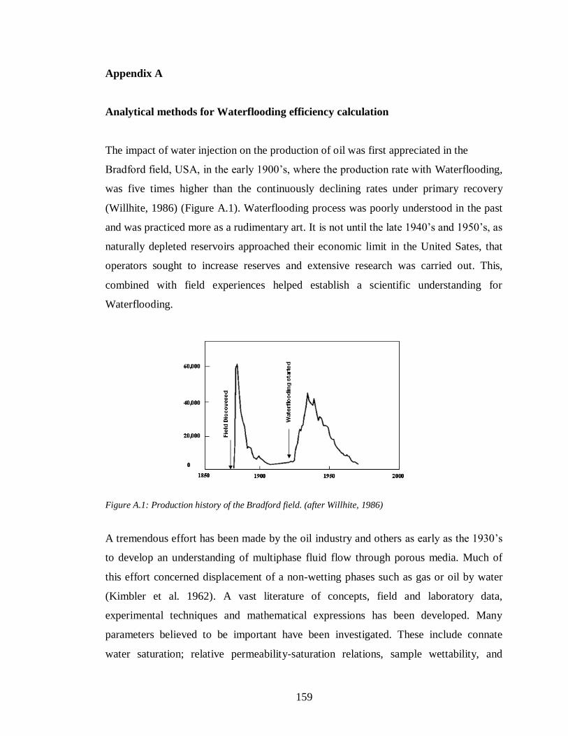
159

Appendix A

Analytical methods for Waterflooding efficiency calculation

The impact of water injection on the production of oil was first appreciated in the

Bradford field, USA, in the early 1900’s, where the production rate with Waterflooding,

was five times higher than the continuously declining rates under primary recovery

(Willhite, 1986) (Figure A.1). Waterflooding process was poorly understood in the past

and was practiced more as a rudimentary art. It is not until the late 1940’s and 1950’s, as

naturally depleted reservoirs approached their economic limit in the United Sates, that

operators sought to increase reserves and extensive research was carried out. This,

combined with field experiences helped establish a scientific understanding for

Waterflooding.

Figure A.1: Production history of the Bradford field. (after Willhite, 1986)

A tremendous effort has been made by the oil industry and others as early as the 1930’s

to develop an understanding of multiphase fluid flow through porous media. Much of

this effort concerned displacement of a non-wetting phases such as gas or oil by water

(Kimbler et al. 1962). A vast literature of concepts, field and laboratory data,

experimental techniques and mathematical expressions has been developed. Many

parameters believed to be important have been investigated. These include connate

water saturation; relative permeability-saturation relations, sample wettability, and

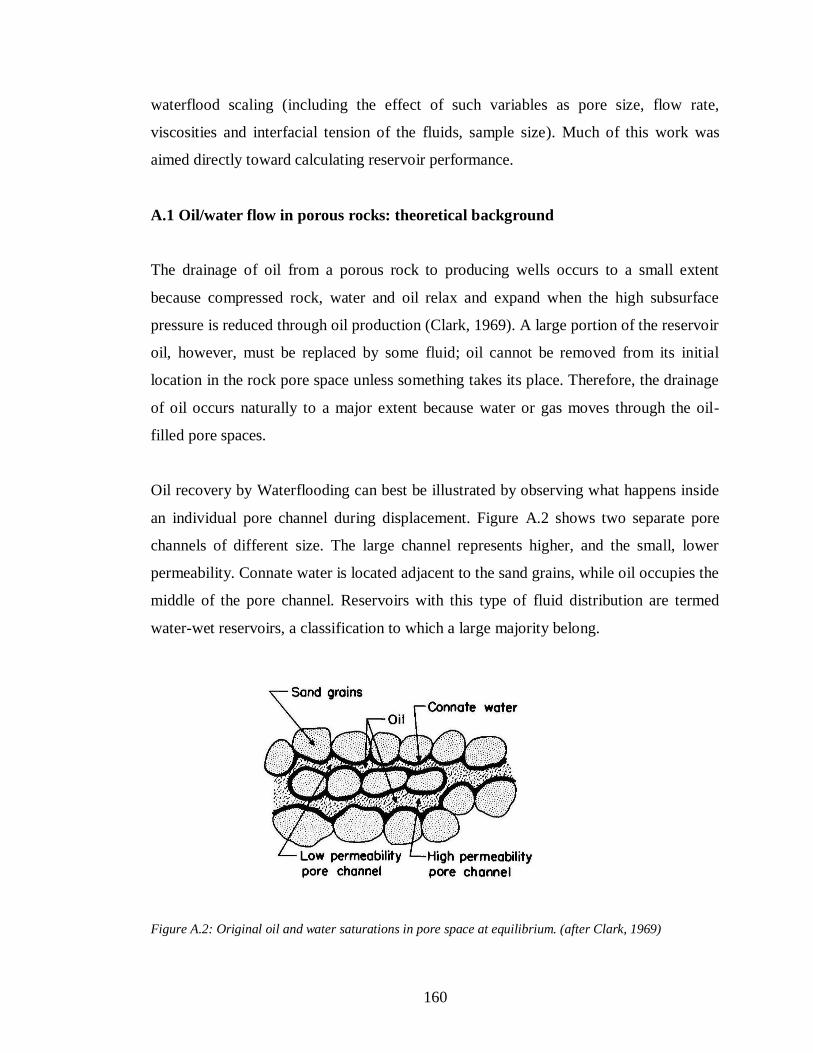
160

waterflood scaling (including the effect of such variables as pore size, flow rate,

viscosities and interfacial tension of the fluids, sample size). Much of this work was

aimed directly toward calculating reservoir performance.

A.1 Oil/water flow in porous rocks: theoretical background

The drainage of oil from a porous rock to producing wells occurs to a small extent

because compressed rock, water and oil relax and expand when the high subsurface

pressure is reduced through oil production (Clark, 1969). A large portion of the reservoir

oil, however, must be replaced by some fluid; oil cannot be removed from its initial

location in the rock pore space unless something takes its place. Therefore, the drainage

of oil occurs naturally to a major extent because water or gas moves through the oil-

filled pore spaces.

Oil recovery by Waterflooding can best be illustrated by observing what happens inside

an individual pore channel during displacement. Figure A.2 shows two separate pore

channels of different size. The large channel represents higher, and the small, lower

permeability. Connate water is located adjacent to the sand grains, while oil occupies the

middle of the pore channel. Reservoirs with this type of fluid distribution are termed

water-wet reservoirs, a classification to which a large majority belong.

Figure A.2: Original oil and water saturations in pore space at equilibrium. (after Clark, 1969)

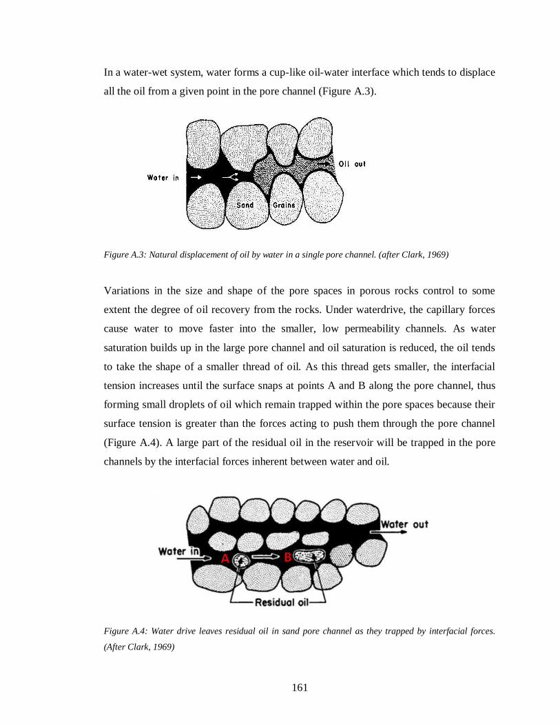
161

In a water-wet system, water forms a cup-like oil-water interface which tends to displace

all the oil from a given point in the pore channel (Figure A.3).

Figure A.3: Natural displacement of oil by water in a single pore channel. (after Clark, 1969)

Variations in the size and shape of the pore spaces in porous rocks control to some

extent the degree of oil recovery from the rocks. Under waterdrive, the capillary forces

cause water to move faster into the smaller, low permeability channels. As water

saturation builds up in the large pore channel and oil saturation is reduced, the oil tends

to take the shape of a smaller thread of oil. As this thread gets smaller, the interfacial

tension increases until the surface snaps at points A and B along the pore channel, thus

forming small droplets of oil which remain trapped within the pore spaces because their

surface tension is greater than the forces acting to push them through the pore channel

(Figure A.4). A large part of the residual oil in the reservoir will be trapped in the pore

channels by the interfacial forces inherent between water and oil.

Figure A.4: Water drive leaves residual oil in sand pore channel as they trapped by interfacial forces.

(After Clark, 1969)

162

The fluid displacement process requires contact between the displacing fluid and the

displaced fluid. The movement of the interface between displacing and displaced fluids

and the breakthrough time associated with the production of injected fluids at producing

wells are indicators of sweep efficiency. One of the simplest and most widely used

methods of estimating the advance of a fluid displacement process is The Buckley-

Leverett displacement theory (Buckley and Leverett, 1942).

In their famous paper published in 1942, Buckley and Leverett described the mechanism

of oil displacement by water (or gas). In fact, the water moves from a region of high

water saturation into one of lower water saturation, removing the oil and converting the

invaded region to one higher in water saturation. The amount of oil displaced by water

during the process of Waterflooding depends upon the relative ease with which the

fluids can move. The readiness with which a fluid flows through sand increases with its

saturation in the sand. At the beginning of the water injection, the oil saturation in the

sand may be high while the water saturation may be low; oil will flow easily and the

water to a small extent only, if at all.

When two immiscible fluids, such as oil and water, are together in contact with a rock

face, one fluid will preferentially adhere to the rock, this fluid is called the wetting fluid

while the other fluid is called the non-wetting fluid. Depending on the wetting properties

of the fluids there are essentially two different types of displacement in two-phase flow

in porous media, drainage and imbibition. The drainage displacement occurs when a

non-wetting invading fluid displaces a wetting fluid. The opposite case, imbibition,

occurs when a wetting fluid displaces a non-wetting fluid. The mechanisms of the

displacements in drainage and imbibition are quite different and the two cases should not

be confused. The displacement of oil by water in a water wet reservoir is, therefore, an

imbibition process, while the displacement of water by oil, in the same type of reservoir

is a drainage process (Figure A.5). As imbibition proceeds, the permeability of the sand

to oil will continuously decrease while the permeability to the water will continuously

increase (Figure A.5), until the final part of the process where huge quantities of water

are injected to displace only a slight amount of additional oil.

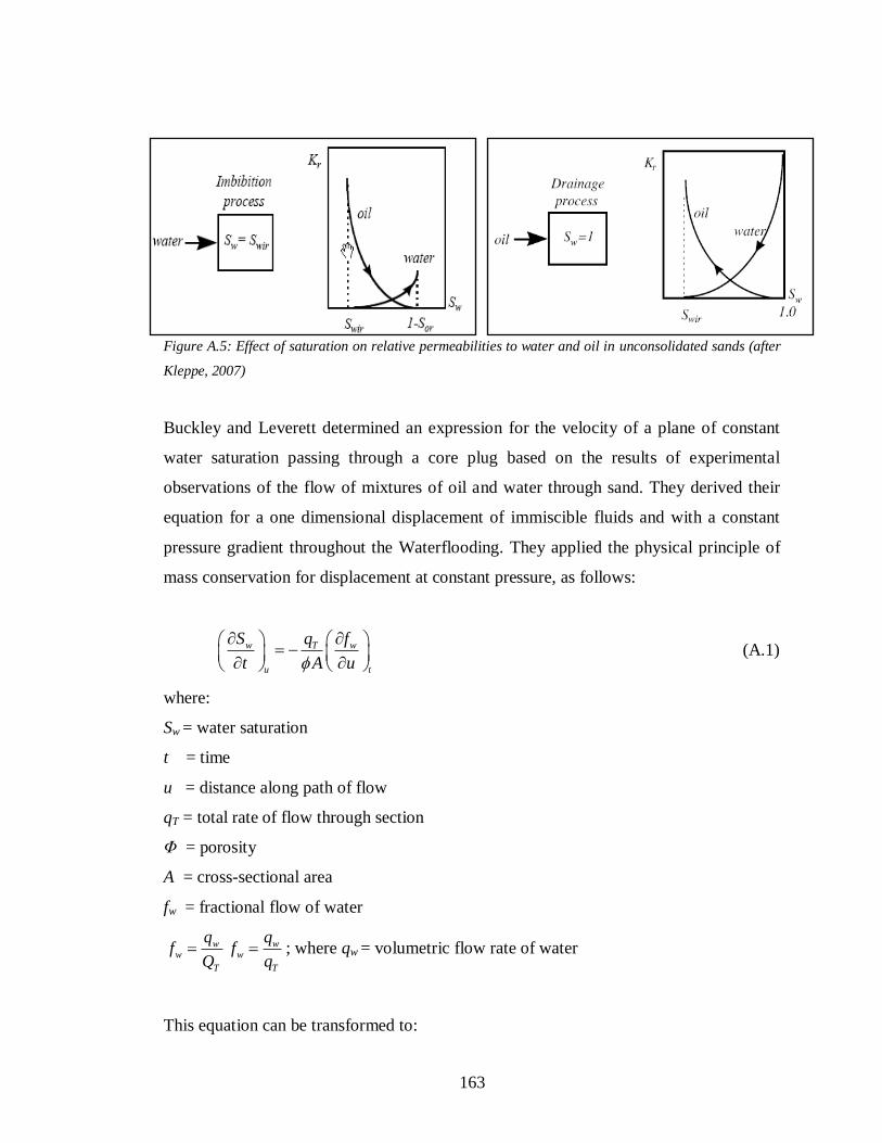
163

Figure A.5: Effect of saturation on relative permeabilities to water and oil in unconsolidated sands (after

Kleppe, 2007)

Buckley and Leverett determined an expression for the velocity of a plane of constant

water saturation passing through a core plug based on the results of experimental

observations of the flow of mixtures of oil and water through sand. They derived their

equation for a one dimensional displacement of immiscible fluids and with a constant

pressure gradient throughout the Waterflooding. They applied the physical principle of

mass conservation for displacement at constant pressure, as follows:

w wT

u t

S fq

t A u

(A.1)

where:

Sw = water saturation

t = time

u = distance along path of flow

qT = total rate of flow through section

Φ = porosity

A = cross-sectional area

fw = fractional flow of water

ww

T

qf

Q w

w

T

qf

q ; where qw = volumetric flow rate of water

This equation can be transformed to:

164

w

wT

S w t

fqu

t A S

(A.2)

This states that the rate of advance of a plane that has a certain fixed saturation is

proportional to the change in composition of the flowing stream caused by a small

change in the saturation of water. By neglecting gravity and capillary pressure difference

effects, fw can be written as:

1

1w

ro w

rw o

fK

K

(A.3)

where Kro and Krw are the permeabilities of the sand to oil and water respectively, while

µo and µw are the viscosities of the two fluids. The relation between the permeabilities

ratio ro

rw

K

K and the water saturation Sw is determined experimentally from the relative

permeabilities curves for the specific sand being flooded. Then the relations between Sw

and fw and between w

w

f

S

and Sw are derived from equation (A.3). Assuming that w

w

f

S

is

only related to Sw, being constant for a fixed Sw, from equation (A.2) it can be seen that

each water saturation Sw moves through the porous rock at a constant velocity v

w w

w

Q dfv

A dS (A.4)

where Qw is the total amount of water entering the system.

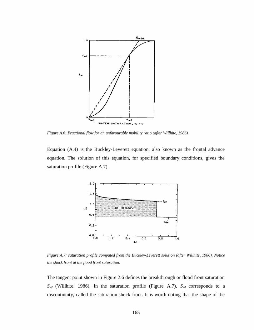
165

Figure A.6: Fractional flow for an unfavourable mobility ratio (after Willhite, 1986).

Equation (A.4) is the Buckley-Leverett equation, also known as the frontal advance

equation. The solution of this equation, for specified boundary conditions, gives the

saturation profile (Figure A.7).

Figure A.7: saturation profile computed from the Buckley-Leverett solution (after Willhite, 1986). Notice

the shock front at the flood front saturation.

The tangent point shown in Figure 2.6 defines the breakthrough or flood front saturation

Swf (Willhite, 1986). In the saturation profile (Figure A.7), Swf corresponds to a

discontinuity, called the saturation shock front. It is worth noting that the shape of the

166

saturation profile between the initial water saturation, Swi and the flood front saturation,

Swf cannot be predicted from the Buckley-Leverett solution, but it is rather approximated

to be one step increase resulting in the shock front illustrated in Figure A.7.

The Buckley-Leverett theory was developed for a one-dimensional core flooding

experiment. Dake (2001) states that since this theory is basically a statement of material

balance, and material balance is zero dimensional, the Buckley-Leverett equation can be

used to describe Waterflooding of a reservoir, quite irrespective of the system’s size or

shape.

A.2 Waterflooding performance calculation

A.2.1 Analytical methods for Waterflooding efficiency calculation

During the first half of the twentieth century, a great deal of research was carried on in

idealized laboratory conditions, from which certain trends and theories have been

indicated. The aim of this research work was to increase the engineers’ knowledge of

recovery processes and to develop techniques for the prediction and monitoring of their

efficiency. Many techniques have been developed for the case of Waterflooding

performance prediction but generally the methodology used for the calculation was

universal and can be summarized in the graph shown in Figure A.8. These early hand-

calculation methods are typified by the zero-dimensional, material balance calculation.

In these analytical calculations, there was no need for detailed geological and production

data as the reservoir was treated as a simple tank having average characteristics and

properties.

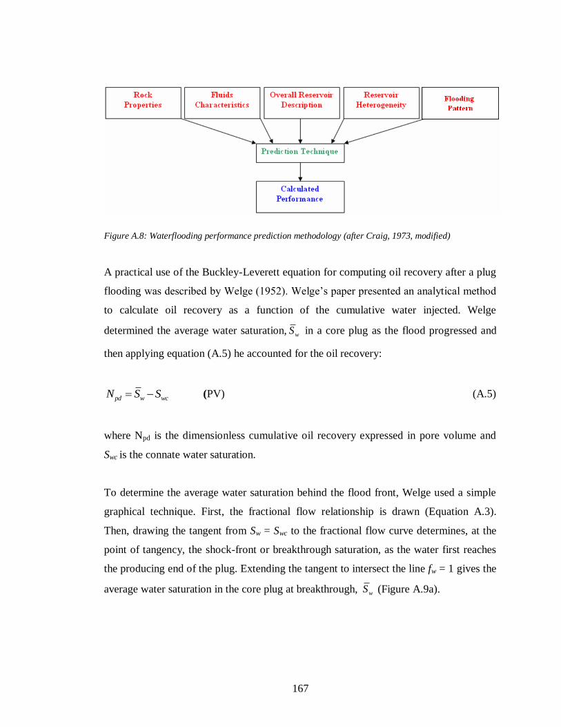
167

Figure A.8: Waterflooding performance prediction methodology (after Craig, 1973, modified)

A practical use of the Buckley-Leverett equation for computing oil recovery after a plug

flooding was described by Welge (1952). Welge’s paper presented an analytical method

to calculate oil recovery as a function of the cumulative water injected. Welge

determined the average water saturation, wS in a core plug as the flood progressed and

then applying equation (A.5) he accounted for the oil recovery:

pd w wcN S S (PV) (A.5)

where Npd is the dimensionless cumulative oil recovery expressed in pore volume and

Swc is the connate water saturation.

To determine the average water saturation behind the flood front, Welge used a simple

graphical technique. First, the fractional flow relationship is drawn (Equation A.3).

Then, drawing the tangent from Sw = Swc to the fractional flow curve determines, at the

point of tangency, the shock-front or breakthrough saturation, as the water first reaches

the producing end of the plug. Extending the tangent to intersect the line fw = 1 gives the

average water saturation in the core plug at breakthrough, wS (Figure A.9a).

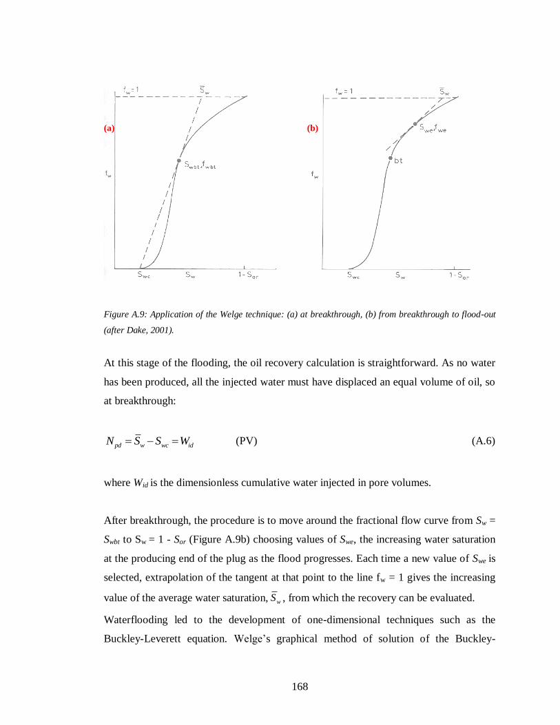
168

(a) (b)

Figure A.9: Application of the Welge technique: (a) at breakthrough, (b) from breakthrough to flood-out

(after Dake, 2001).

At this stage of the flooding, the oil recovery calculation is straightforward. As no water

has been produced, all the injected water must have displaced an equal volume of oil, so

at breakthrough:

pd w wc idN S S W (PV) (A.6)

where Wid is the dimensionless cumulative water injected in pore volumes.

After breakthrough, the procedure is to move around the fractional flow curve from Sw =

Swbt to Sw = 1 - Sor (Figure A.9b) choosing values of Swe, the increasing water saturation

at the producing end of the plug as the flood progresses. Each time a new value of Swe is

selected, extrapolation of the tangent at that point to the line fw = 1 gives the increasing

value of the average water saturation, wS , from which the recovery can be evaluated.

Waterflooding led to the development of one-dimensional techniques such as the

Buckley-Leverett equation. Welge’s graphical method of solution of the Buckley-

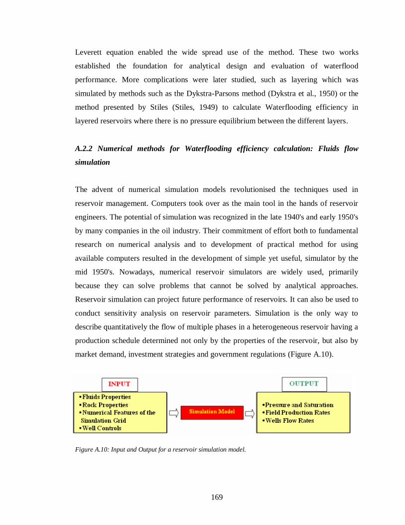
169

Leverett equation enabled the wide spread use of the method. These two works

established the foundation for analytical design and evaluation of waterflood

performance. More complications were later studied, such as layering which was

simulated by methods such as the Dykstra-Parsons method (Dykstra et al., 1950) or the

method presented by Stiles (Stiles, 1949) to calculate Waterflooding efficiency in

layered reservoirs where there is no pressure equilibrium between the different layers.

A.2.2 Numerical methods for Waterflooding efficiency calculation: Fluids flow

simulation

The advent of numerical simulation models revolutionised the techniques used in

reservoir management. Computers took over as the main tool in the hands of reservoir

engineers. The potential of simulation was recognized in the late 1940's and early 1950's

by many companies in the oil industry. Their commitment of effort both to fundamental

research on numerical analysis and to development of practical method for using

available computers resulted in the development of simple yet useful, simulator by the

mid 1950's. Nowadays, numerical reservoir simulators are widely used, primarily

because they can solve problems that cannot be solved by analytical approaches.

Reservoir simulation can project future performance of reservoirs. It can also be used to

conduct sensitivity analysis on reservoir parameters. Simulation is the only way to

describe quantitatively the flow of multiple phases in a heterogeneous reservoir having a

production schedule determined not only by the properties of the reservoir, but also by

market demand, investment strategies and government regulations (Figure A.10).

Figure A.10: Input and Output for a reservoir simulation model.

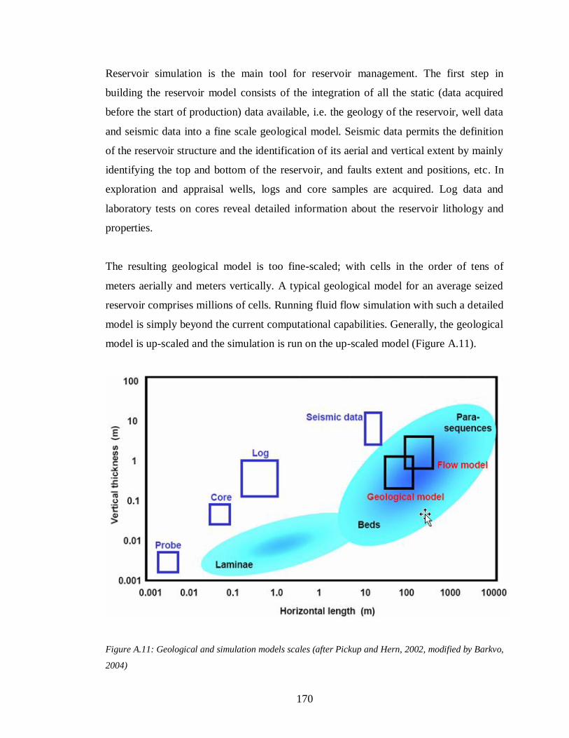
170

Reservoir simulation is the main tool for reservoir management. The first step in

building the reservoir model consists of the integration of all the static (data acquired

before the start of production) data available, i.e. the geology of the reservoir, well data

and seismic data into a fine scale geological model. Seismic data permits the definition

of the reservoir structure and the identification of its aerial and vertical extent by mainly

identifying the top and bottom of the reservoir, and faults extent and positions, etc. In

exploration and appraisal wells, logs and core samples are acquired. Log data and

laboratory tests on cores reveal detailed information about the reservoir lithology and

properties.

The resulting geological model is too fine-scaled; with cells in the order of tens of

meters aerially and meters vertically. A typical geological model for an average seized

reservoir comprises millions of cells. Running fluid flow simulation with such a detailed

model is simply beyond the current computational capabilities. Generally, the geological

model is up-scaled and the simulation is run on the up-scaled model (Figure A.11).

Figure A.11: Geological and simulation models scales (after Pickup and Hern, 2002, modified by Barkvo,

2004)

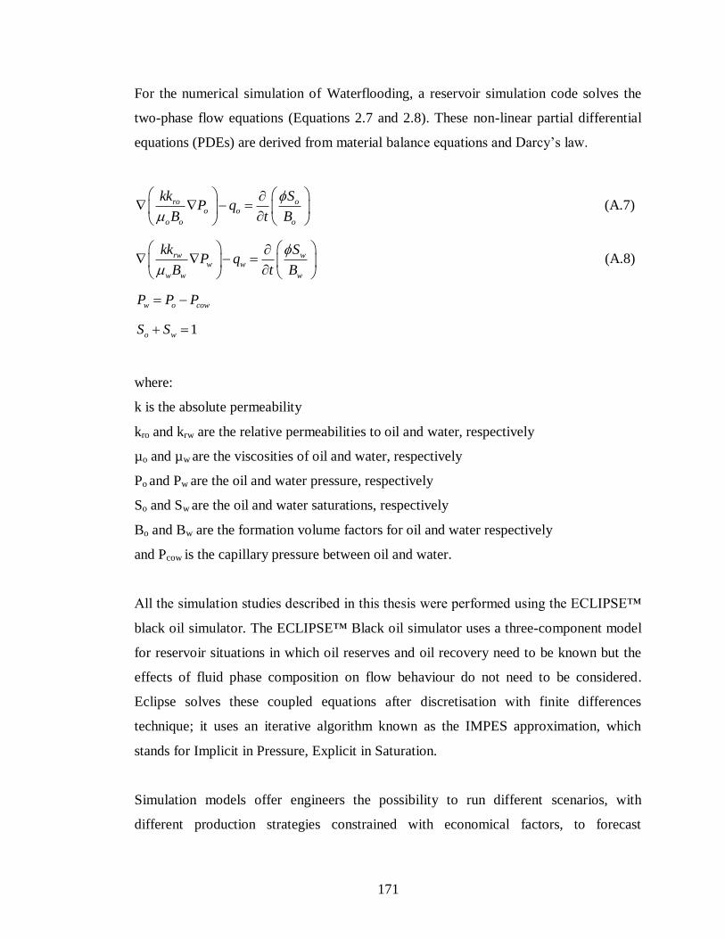
171

For the numerical simulation of Waterflooding, a reservoir simulation code solves the

two-phase flow equations (Equations 2.7 and 2.8). These non-linear partial differential

equations (PDEs) are derived from material balance equations and Darcy’s law.

ro oo o

o o o

kk SP q

B t B

(A.7)

rw ww w

w w w

kk SP q

B t B

(A.8)

w o cowP P P

1o wS S

where:

k is the absolute permeability

kro and krw are the relative permeabilities to oil and water, respectively

µo and µw are the viscosities of oil and water, respectively

Po and Pw are the oil and water pressure, respectively

So and Sw are the oil and water saturations, respectively

Bo and Bw are the formation volume factors for oil and water respectively

and Pcow is the capillary pressure between oil and water.

All the simulation studies described in this thesis were performed using the ECLIPSE™

black oil simulator. The ECLIPSE™ Black oil simulator uses a three-component model

for reservoir situations in which oil reserves and oil recovery need to be known but the

effects of fluid phase composition on flow behaviour do not need to be considered.

Eclipse solves these coupled equations after discretisation with finite differences

technique; it uses an iterative algorithm known as the IMPES approximation, which

stands for Implicit in Pressure, Explicit in Saturation.

Simulation models offer engineers the possibility to run different scenarios, with

different production strategies constrained with economical factors, to forecast

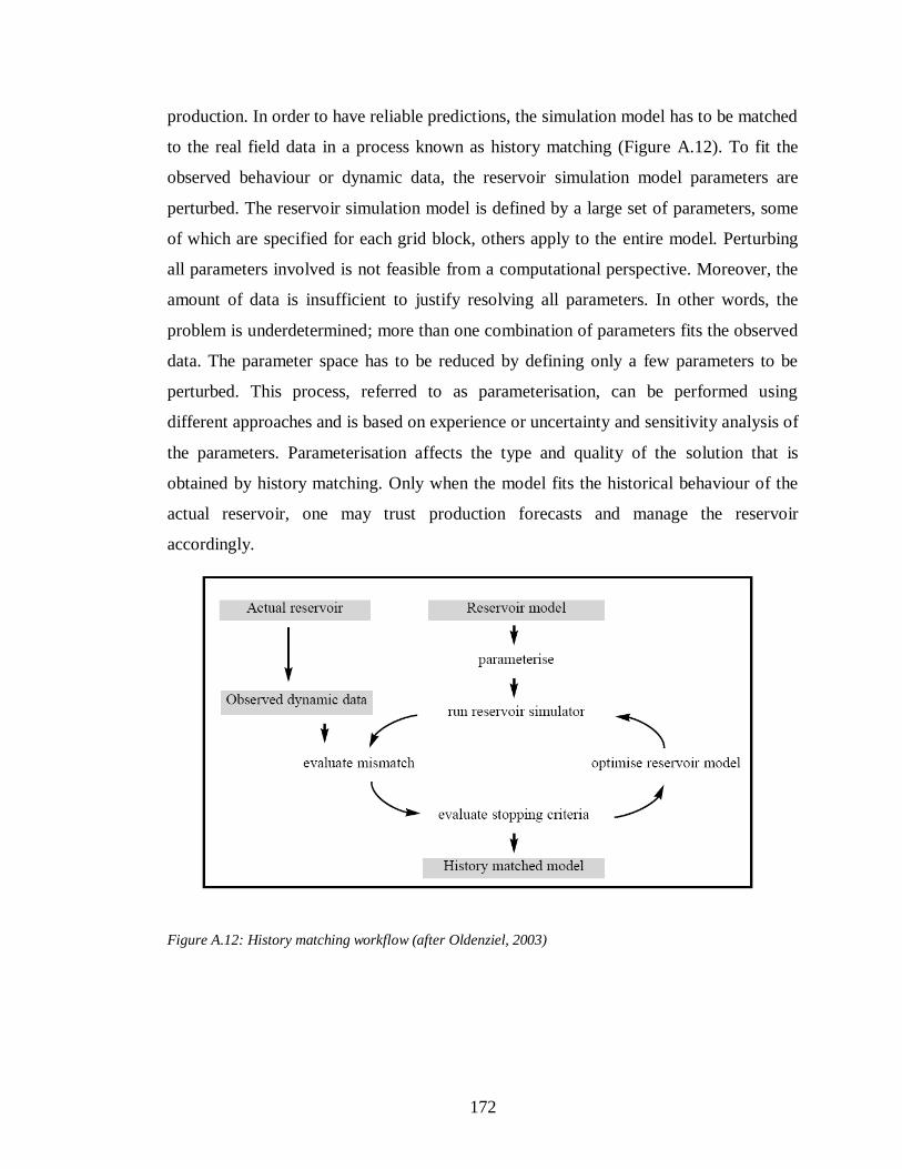
172

production. In order to have reliable predictions, the simulation model has to be matched

to the real field data in a process known as history matching (Figure A.12). To fit the

observed behaviour or dynamic data, the reservoir simulation model parameters are

perturbed. The reservoir simulation model is defined by a large set of parameters, some

of which are specified for each grid block, others apply to the entire model. Perturbing

all parameters involved is not feasible from a computational perspective. Moreover, the

amount of data is insufficient to justify resolving all parameters. In other words, the

problem is underdetermined; more than one combination of parameters fits the observed

data. The parameter space has to be reduced by defining only a few parameters to be

perturbed. This process, referred to as parameterisation, can be performed using

different approaches and is based on experience or uncertainty and sensitivity analysis of

the parameters. Parameterisation affects the type and quality of the solution that is

obtained by history matching. Only when the model fits the historical behaviour of the

actual reservoir, one may trust production forecasts and manage the reservoir

accordingly.

Figure A.12: History matching workflow (after Oldenziel, 2003)

173

Appendix B

Seismic characteristics of turbidite reservoirs

Advances in seismic reflection imaging have been a crucial element in the development

of deepwater exploration. It significantly reduced the geological risk to acceptable levels

(Rudolph, 2001). Advanced seismic imaging techniques, such as prestack depth

migration (PSDM) have become critical tools for imaging deepwater traps during both

discovery and appraisal allowing the imaging of the reservoir architecture and field

extent in geologically complex settings (Weimer, 2004).

Different turbidite systems have different seismic stratigraphic responses. Gravel-rich

turbidite systems occur near highland areas associated with fault-bounded basins.

Deposition in proximal areas is by avalanching and debris flow whereas turbidite

processes dominate toward the centre of the basin as flows become more fluidized. This

results in poorly sorted deposits at the edges of the basins and well sorted channels

basinward. They appear on 2D seismic as externally wedge shaped and show internally

slightly diverging reflections toward the fault and converging reflections basinward. On

3D seismic, the complexity of sediments delivery systems is more accentuated and

channels and chutes sometimes can be resolved. Figure B.1 shows a seismic section and

the corresponding schematic of the Upper Jurassic Brae Field complex in the North Sea.

The schematic cross-section shows abrupt lateral and vertical changes in stratigraphic

units which are difficult to pick on seismic sections. Wireline logs are difficult to

correlate making reservoir prediction and production hard and uncertain. This

uncertainty can be reduced with 3D seismic interpretation.

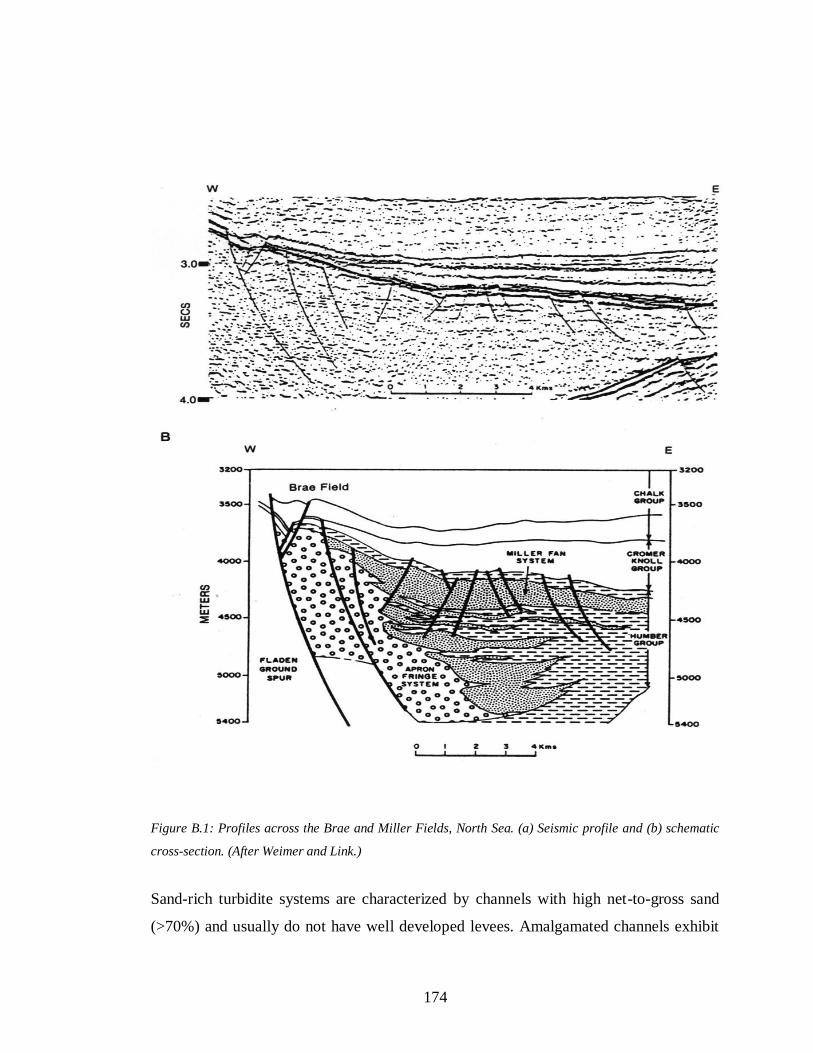
174

Figure B.1: Profiles across the Brae and Miller Fields, North Sea. (a) Seismic profile and (b) schematic

cross-section. (After Weimer and Link.)

Sand-rich turbidite systems are characterized by channels with high net-to-gross sand

(>70%) and usually do not have well developed levees. Amalgamated channels exhibit

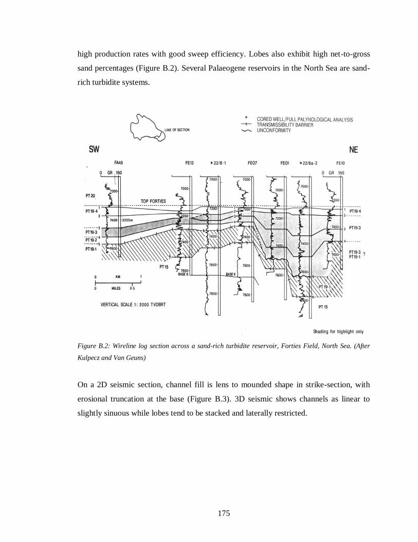
175

high production rates with good sweep efficiency. Lobes also exhibit high net-to-gross

sand percentages (Figure B.2). Several Palaeogene reservoirs in the North Sea are sand-

rich turbidite systems.

Figure B.2: Wireline log section across a sand-rich turbidite reservoir, Forties Field, North Sea. (After

Kulpecz and Van Geuns)

On a 2D seismic section, channel fill is lens to mounded shape in strike-section, with

erosional truncation at the base (Figure B.3). 3D seismic shows channels as linear to

slightly sinuous while lobes tend to be stacked and laterally restricted.

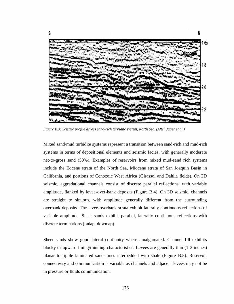
176

Figure B.3: Seismic profile across sand-rich turbidite system, North Sea. (After Jager et al.)

Mixed sand/mud turbidite systems represent a transition between sand-rich and mud-rich

systems in terms of depositional elements and seismic facies, with generally moderate

net-to-gross sand (50%). Examples of reservoirs from mixed mud-sand rich systems

include the Eocene strata of the North Sea, Miocene strata of San Joaquin Basin in

California, and portions of Cenozoic West Africa (Girassol and Dahlia fields). On 2D

seismic, aggradational channels consist of discrete parallel reflections, with variable

amplitude, flanked by levee-over-bank deposits (Figure B.4). On 3D seismic, channels

are straight to sinuous, with amplitude generally different from the surrounding

overbank deposits. The levee-overbank strata exhibit laterally continuous reflections of

variable amplitude. Sheet sands exhibit parallel, laterally continuous reflections with

discrete terminations (onlap, downlap).

Sheet sands show good lateral continuity where amalgamated. Channel fill exhibits

blocky or upward-fining/thinning characteristics. Levees are generally thin (1-3 inches)

planar to ripple laminated sandstones interbedded with shale (Figure B.5). Reservoir

connectivity and communication is variable as channels and adjacent levees may not be

in pressure or fluids communication.

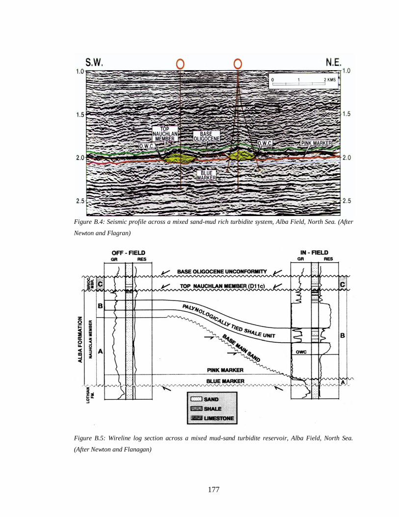
177

Figure B.4: Seismic profile across a mixed sand-mud rich turbidite system, Alba Field, North Sea. (After

Newton and Flagran)

Figure B.5: Wireline log section across a mixed mud-sand turbidite reservoir, Alba Field, North Sea.

(After Newton and Flanagan)

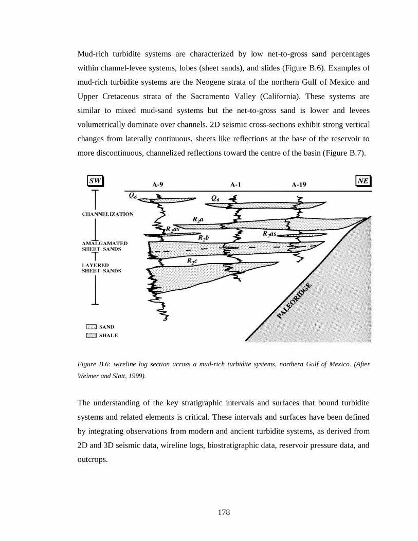
178

Mud-rich turbidite systems are characterized by low net-to-gross sand percentages

within channel-levee systems, lobes (sheet sands), and slides (Figure B.6). Examples of

mud-rich turbidite systems are the Neogene strata of the northern Gulf of Mexico and

Upper Cretaceous strata of the Sacramento Valley (California). These systems are

similar to mixed mud-sand systems but the net-to-gross sand is lower and levees

volumetrically dominate over channels. 2D seismic cross-sections exhibit strong vertical

changes from laterally continuous, sheets like reflections at the base of the reservoir to

more discontinuous, channelized reflections toward the centre of the basin (Figure B.7).

Figure B.6: wireline log section across a mud-rich turbidite systems, northern Gulf of Mexico. (After

Weimer and Slatt, 1999).

The understanding of the key stratigraphic intervals and surfaces that bound turbidite

systems and related elements is critical. These intervals and surfaces have been defined

by integrating observations from modern and ancient turbidite systems, as derived from

2D and 3D seismic data, wireline logs, biostratigraphic data, reservoir pressure data, and

outcrops.

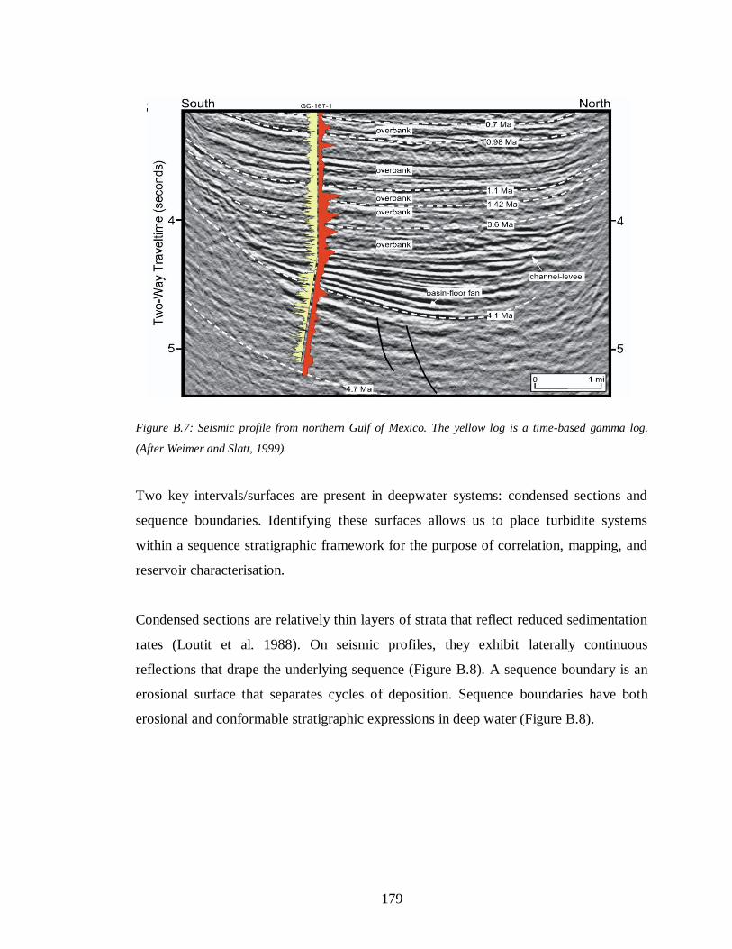
179

Figure B.7: Seismic profile from northern Gulf of Mexico. The yellow log is a time-based gamma log.

(After Weimer and Slatt, 1999).

Two key intervals/surfaces are present in deepwater systems: condensed sections and

sequence boundaries. Identifying these surfaces allows us to place turbidite systems

within a sequence stratigraphic framework for the purpose of correlation, mapping, and

reservoir characterisation.

Condensed sections are relatively thin layers of strata that reflect reduced sedimentation

rates (Loutit et al. 1988). On seismic profiles, they exhibit laterally continuous

reflections that drape the underlying sequence (Figure B.8). A sequence boundary is an

erosional surface that separates cycles of deposition. Sequence boundaries have both

erosional and conformable stratigraphic expressions in deep water (Figure B.8).

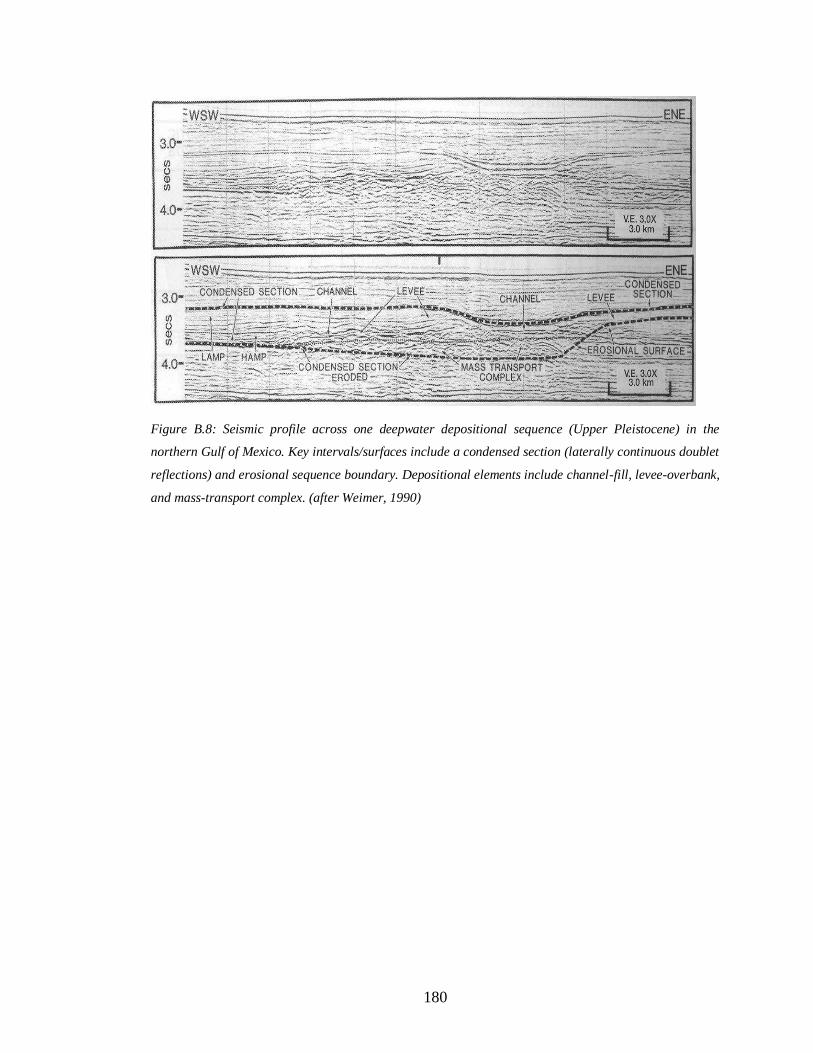
180

Figure B.8: Seismic profile across one deepwater depositional sequence (Upper Pleistocene) in the

northern Gulf of Mexico. Key intervals/surfaces include a condensed section (laterally continuous doublet

reflections) and erosional sequence boundary. Depositional elements include channel-fill, levee-overbank,

and mass-transport complex. (after Weimer, 1990)

181

Appendix C

A brief history of petroleum use in human civilisation

Petroleum is not a new substance in human civilisation. Ancient people discovered many

practical uses for petroleum substances (Forbes, 1964). Ancient civilizations from

northern Iraq, south-west Iran and the Dead Sea area extensively used the abundant

natural resources of petroleum, found in the form of natural bitumen deposits, oil

seepage and liquid oil shows, until the Neolithic period (7,000 – 6,000 BC). Evidence of

earlier use has been documented in the Syrian Desert (Boëda et al., 1996), where

bitumen-coated flint implements, dated to 40,000 BC (Mousterian period), have been

unearthed.

Bitumen was largely used in Mesopotamia and Elam as mortar in the construction of

palaces (e.g. the Darius Palace in Susa), temples, ziggurats (e.g. the Tower of Babel in

Babylon), terraces (e.g. the Hanging Gardens of Babylon) and exceptionally for roadway

coating (e.g. the processional way of Babylon). Since the Neolithic, bitumen served to

waterproof containers (baskets, jars, storage pits), wooden pots, palaces grounds, palm

roofs, etc. Mats, sarcophagi, coffins and jars, used for funeral practices, were often

covered and sealed with bitumen (Connan, 1999).

Bitumen was also considered as a powerful remedy in medical practice, especially as a

disinfectant and insecticide, and was used by the ancient Egyptians to prepare mixtures

to embalm the corpses of their dead during the mummification process. The use of

petroleum substances in the ancient times was not limited to the Middle East area,

ancient Far East civilisations, such as in China and in Japan, used oil for lighting and for

medical purposes. Mediterranean civilisations used bitumen in many of their every day

life tasks.

182

The modern history of the petroleum industry began when the process of refining

kerosene from raw coal was discovered by Abraham Pinoe Gesner in the year 1846.

Then there was literally no looking back for the growth of petroleum industry

throughout the world. The first Russian refinery was built at Baku during the year 1861

and it accounted for around 90% of the world oil production.

During the 1800s the growth was gradual and quite slow. Before the 1850s, people often

used whale oil for light. When whale oil became scarce, people began looking for other

oil sources: kerosene. Colonel Edwin Drake drilled the first successful oil well in

Titusville, Pennsylvania in 1859 looking for a source of kerosene to be used for lighting

fuel. This primary market for oil had begun to disappear when Thomas Edison invented

the light bulb and created the electrical generation industry.

For most of the 19th century, gasoline was simply a by product of the production of

kerosene, with few commercial uses, but after the internal combustion engine was

invented in 1896, there was a surge in the demand for petroleum products. The outbreak

of World War I in 1914 changed the role of petroleum in the world forever. Motorized

transport began to dramatically change the nature of war. The development of the

airplane and of the tank, which was first used at the Battle of the Somme in

1918, provided both mobility and power that was unprecedented in the history of

warfare; in some ways, oil was more critical to military success than ammunition.

The sale of oil became an important industry by the early 1900s. Oil fields were also

discovered in places such as Canada, Iran, Mexico, Venezuela and Peru. At that same

time, the automobile industry began to grow rapidly, opening up an enormous market for

gasoline. New more efficient refining processes were invented and led to the production

of more gasoline out of each barrel of crude oil. Farming productivity after the war was

greatly improved by tractors and other oil-fuelled machinery. Similarly during World

War II, the oil industry proved that it could boost production quickly and create

specialized new products for military needs, such as high-octane fuel for airplanes and

raw materials for synthetic rubber.

http://www.bookrags.com/research/petroleum-wsd/


183

By the 1950s, oil had replaced coal as the world’s most important fuel, just as coal had

replaced wood 150 years earlier. In addition to supplying the automotive market, oil had

displaced coal as the major railroad fuel. Even more quickly, oil took coal's place as a

shipping fuel. Oil also began to compete with coal in certain industrial applications and

even, to some extent, in power generation.


184

References

Aki, A. and P.G. Richards, 1980, Quantitative seismology: Theory and methods: W.H.

Freeman and Company.

Amini, H., 2009, ETLP Meeting, November 2009, personnel communication

Backus, G. E. (1962). Long-wave elastic anisotropy produced by horizontal layering.

67:4427–4440.

Bakke, K., Gjelberg, J. and Petersen, S.A., 2007, Compound seismic modelling of the

Ainsa II turbidite system, Spain: Application to deep-water channel systems offshore

Angola. Marine and Petroleum Geology 25 (2008) 1058-1073

Batzle, M. and Wang, Z., 1992, Seismic properties of pore fluids. Geophysics,

57(11):1396–1408.

Bentham, P.A., Burbank, D.W., Puigdefabregas, C., 1992, Temporal and spatial controls

on the alluvial architecture of an axial drainage system: late Eocene Escanilla Formation,

southern Pyrenean forland basin, Spain. Basin Research 4, 335–352.

Berryman, J. (1999). Tutorial: Origin of Gassmann’s equations. Geophysics, 64:1627–

1629.

Berryman, J. and Milton, G. (1991). Exact results for generalized Gassmann’s equations

in composite porous media with two constituents. Geophysics, 56:1950–1960.

Biot, M. (1956). Theory of propagation of elastic waves in a fluid saturated porous solid,

Parts I and II. The journal of the Acoustic Society of America, 28:168–191.

185

Boëda, E., Connan, J., Dessort, D., Muhesen, S., Mercier, N., Valadas, H. & Tisnerat,

N., 1996, Bitumen as a hafting material on Middle Palaeolithic artefacts. Nature 380,

336-338.

Bourgeois, A., Labat, K., Euzen, T., Le Bras,C., 2005, How to build a geological and

geophysical realistic synthetic seismic data set for benchmarking reservoirs studies?

SEG 2005 Annual Meeting, Houston, Texas, USA.

Brawis, J.H., McPherson, J.G. and Studlick, J.R., 1990, Sandstone petroleum reservoirs,

Springer-Verlag New York Inc.

Buckley, S.E. and Leverett, M.C., 1942, Mechanism of Fluid Displacement in Sands,

Transactions, AIME, 1942, Vol.146:107.

Byerley, G., Pederson, J., Roervik, K.O., Ranaweera, K. and Janssen, A., 2006,

Reducing risk and monitoring water injection using time-lapse (4D) seismic at the

Ekofisk field. SEG International Exposition and Annual Meeting, New Orleans

Chapin, M.A, P. Davis, J.L. Gibson, and H.S. Pettingill, 1994, Reservoir architecture of

turbidite sheet sandstones in laterally extensive outcrops, Ross Formation, western

Ireland, in P. Weimer, A.H. Bouma, and B.F. Perkins, eds., Submarine fans and turbidite

systems: Gulf Coast Section-SEPM Foundation 15th Annual Research Conference, 53-

68.

Connan, J., 1999, Use and trade of bitumen in antiquity and prehistory: molecular

archaeology reveals secrets of past civilizations, Philosophical Transactions of the Royal

Society B: Biological Sciences, 1999 January 29; volume 354, pp.: 33–50

Connan, J. & Deschesne, O., 1995, Archaeological bitumen: identification, origins and

uses of an ancient near eastern material. Mat. Res. Soc. Symp. Proc. 267, 683-720.

186

Craig Jr., F.F., 1973, Engineering Waterfloods for Improved Oil Recovery

SPE Distinguished Lecture, SPE 4425-MS

Dake L.P., 2001, The Practice of Reservoir Engineering (revised edition), Elsevier.

Domes, F., MacBeth, C., and Brain, J., 2009, The Influence of Overburden on Time-

Lapse Saturation Interpretation. 71th EAGE Meeting, page Y002, Amsterdam,

Netherlands.

Dreyer, T., Corregidor, J., Arbues, P., Puigdefabregas, C., 1999, Architecture of the

tectonically influenced Sobrarbe deltaic complex in the Ainsa Basin, northern Spain.

Sedimentary Geology 127, 127–169.

Dykstra, H. and Parsons, R.L, 1950, The Prediction of Oil Recovery by Waterflood,

Secondary Recovery of Oil in the U.S., API, 160

Falcone, G., Gosselin, O., Maire, F., Marrauld, J., and Zhakupov, M. (2004). Petroelastic

modelling as key element of 4D History Matching: A Field Example (SPE 90466). In

SPE Annual Technical Conference and Exhibition, Houston, Texas

Floricich, M., 2006, An engineering-consistent approach for pressure and saturation

estimation from time-lapse seismic data. PhD thesis, Heriot Watt University.

Fontana, D., Zuffa, G.G., Garzanti, E., 1989, The interaction of eustacy and tectonism

from provenance studies of the Eocene Heocho Group

Forbes, R. J., 1964, Bitumen and petroleum in Antiquity. In Studies in Ancient

Technology, 2nd

edition. vol. 1, pp. 11-23.

https://www.spe.org/elibrary/servlet/spepreview?id=00004425&speCommonAppContext=ELIBRARY

187

Freund, D., 1992, Ultrasonic compressional and shear velocities in dry clastic rocks as a

function of porosity, clay content and confining pressure. Geophysical Journal

International, 108:125–135.

Garfield, T.R., D.C. Jennette, F.J. Goulding, and D.K. Sickafoose, 1998, An integrated

approach to deepwater reservoir prediction. AAPG International Conference and

Exhibition, Expanded Abstracts volume, 278-279.

Gassmann, F., 1951, Uber die Elastizitt Poroser Medien: Vierteljahrsschrift der

Naturforschenden Gesellschaft in Zurich, 96, 1–23.

Hamada, G.M., 2004, Reservoir Fluids Identification Using Vp/Vs Ratio, Oil & Gas

Science and Technology – Rev. IFP, Vol. 59 (2004), No. 6, pp. 649-654

Han, D., Nur, A., and Morgan, D., 1986, Effects of porosity and clay content on wave

velocities in sandstones. Geophysics, 51(11):2093–2107.

Jager et al., 1993, Evolution of Palaeogene submarine fans of the North Sea in space and

time, Petroleum Geology of Northwest Europe: Proceedings of the Fourth Conference,

The Geological Society, London.

Kahar, Y., and Anno, P. D., 2006, Fluid flow phenomena from 4D interpretation,

Heidrun Field, Norwegian North Sea. SEG Annual Meeting, New Orleans 2006.

Kimbler, O.K., Caudle, B.H. and Hutchinson Jr., C.A., 1962, A Fresh Look at

Waterflood Theory and Practice, SPE 365-MS 1962

Kleppe, J., Review of relative permeabilities and capillary pressure, Reservoir Recovery

Techniques, Handout note 3, Norwegian University of Science and Technology,

Department of Petroleum Engineering and Applied Geophysics.

http://www.spe.org/elibrary/servlet/spepreview?id=00000365&speCommonAppContext=ELIBRARY

http://www.spe.org/elibrary/servlet/spepreview?id=00000365&speCommonAppContext=ELIBRARY

188

Koster, K., Gabriels, P., Hartung, M., Verbeek, J., Deinum, G. and Staples, R., 2000,

Time-lapse seismic surveys in the North Sea and their business impact.

Kulpecz and van Geuns, 1990, Geological modelling of a turbidite reservoir, Forties

Fields, North Sea, Sandstone Petroleum Reservoirs, Springer-Verlag

Landro, M., Solheim, O.A., Hilde, E., Ekren, B.O. and Stronem, LK., 1999, The

Gullfaks 4D seismic study. Petroleum Geosciences, Volume 5, 1999, pp. 213-226

Loutit, T.S., J. Hardenbol, P.R. Vail, and G.R. Baum, 1988, Condensed sections: the key

to age determination and correlation of continental margin sequences, in C.K. Wilgus,

B.S. Hastings and C.G. St. C. Kendall, editions, sea-level changes: An integrated

approach: SEPM Special Publication 42, 183-213.

Lumley, D., 2004, Business and technology challenges for 4D seismic reservoir

monitoring. The Leading Edge, 23(11):1166–1168.

Lumley, D.E. and Behrens, R.A., 1998, Practical issues of 4D seismic reservoir

monitoring: What an engineer needs to know, SPE Reservoir Evaluation and

Engineering, 1998.

MacBeth, C., 2004, A classification for the pressure-sensitivity properties of a sandstone

rock frame. Geophysics, Vol 69, No 2 (March-April 2004); P. 497-510.

MacBeth, C., Soldo, J., and Floricich, M., 2004, Going quantitative with 4D seismic.

SEG International Exposition and Annual Meeting, Denver, Colorado.

MacBeth, C., Stephen, K. and McInally, A., 2005, The 4D seismic signature of oil-water

contact movement due to natural production in a stacked turbidite reservoir. Geophysical

prospecting, 2005, 53, 183-203.

189

MacBeth, C., HajNasser, Y., Stephen, K., and Gardiner, A., 2010, Exploring the effect

of meso-scale shale beds on the reservoir’s overall stress sensitivity to seismic waves.

Geophysical prospecting, in press

Marsh, M., 2004, 4D in reservoir management - Successes and Challenges. IOR Views

e-Newsletter, 8.

Marsh, J.M., Whitcombe, D.N., Raikes, S.A., Parr, R.S. and Nash, T., 2002, BP’s

increasing systematic use of time-lapse seismic technology. Petroleum Geoscience,

Volume 9, pp. 7-13

Mutti, E. and W.R. Normark, 1987, Comparing examples of modern and ancient

turbidite systems: Problems and concepts, in J.K. Leggett and G.G. Zuffa, eds., Marine

clastic sedimentology: London, Graham and Trotman,1-38.

Mutti, E. and W.R. Normark, 1991, An integrated approach to the study of turbidite

systems, in P. Weimer and M. H. Link, eds, Seismic facies and sedimentary processes of

submarine fans and turbidite system: New York, Springer-Verlag, 75-106.

Newton and Flanagan, 1993, The Alba Field: evolution of the depositional model,

Petroleum Geology of Northwest Europe: Proceedings of the Fourth Conference, The

Geological Society, London.

Oldenziel, T., 2003, Time lapse seismic within reservoir engineering, PhD thesis, Delft

University of technology, 2003.

Philip, J.R., 1991, Soil, natural science, and models. Soil Science Journal, Volume 151,

January, pp 91-98.

Pickering, K.T., Corregidor, J., 2000, 3D Reservoir scale study of Eocene confined

Submarine Fans, south Central Spanish Pyrenees. Deep Water Reservoirs of the World.

190

Gulf Coast Section, Society of Economic Palaeontologists and Mineralogists,

Foundation 20th Annual Bob F. Perkins Research Conference, Houston, TX, pp. 776–

781

Pickering, K.T., Corregidor, J., 2005, Mass-transport complexes (MTCs) and tectonic

control on basin-floor submarine fans, middle Eocene, south Spanish Pyrenees. Journal

of Sedimentary Research 75, 761–783.

Rauch, J., 2001, The new old economy: Oil, computers, and the reinvention of the earth,

The Atlantic, January 2001

Reading, H.G. and M. Richards, 1994, Turbidite systems in deep-water basin margins

classified by grain size and feeder system: AAPG Bulletin, 78, 792-822.

Rudolph, K. W., 2001, DHI/AVO analysis best practices: A worldwide analysis: AAPG

Distinguished Lecturer abstract (www.aapg.org)

Schinelli, M., 2006, Using complex seismic attributes to improve 4D visibility of fluids

contact movement, SEG Annual Meeting, New Orleans 2006.

Smith, P., 1998, Reservoir characterization, modelling, and fluid-flow simulation in

Developing and Managing Turbidite Reservoirs: Case Histories and Experiences.

Staples, R., Cook, A., Braisby, J., Mabillard, A. and Rowbotham, P.S. 2006: Integration

of 4D Seismic Data and the Dynamic Reservoir Model - Revealing New Targets in

Gannet C, EAGE 68th Conference & Exhibition — Vienna, Austria, 2006

Staples, R., Stammeijer, J., Jones, S., Brain, J., Smit, F. and Hatchell, P., 2006, Time-

Lapse (4D) Seismic Monitoring - Expanding Applications. 2006 CSPG – CSEG –

CWLS Convention.

http://www.aapg.org/

191

Stiles, W.E., 1949, Use of Permeability Distribution in Water Flood Calculations,

Transactions, AIME, volume 186:9.

Tad M. Smith, Carl H. Sondergeldz, and Chandra S. Raiz, 2003, Gassmann fluid

substitutions: A tutorial. Geophysics, Vol. 68, No. 2 (March-April 2003); P. 430–440.

Thore, P. 2006, Accuracy and limitations in seismic modeling of reservoir, SEG Annual

Meeting, New Orleans 2006.

Thurmond, J.B., Løseth, T.M., Rivenæs, J.C., Martinsen, O.J., Aiken, C., Xu, X., 2008,

Using Outcrop Data in the 21st Century – New methods and applications, with example

from the Ainsa Turbidite System, Ainsa, Spain. AAPG Atlas of Deep Water Outcrops,

in press.

Wang, Z., Hirsche, W. K. and Sedgwick, G., 1991, Seismic monitoring of water floods?

A petrophysical study. SEG 60th

Annual Meeting.

Wang, Z. and Nur, A., 1986, Effect of temperature on wave velocities in sands and

sandstones with heavy hydrocarbons (SPE 15646), SPE Annual Technical Conference

and Exhibition, New Orleans, Louisiana.

Wang, Z., Batzle, M., and Nur, A., 1990, Effect of different pore fluids on seismic

velocities in rocks, Canadian Journal of Exploration Geophysics, 26(1 - 2):104–112.

Waggoner, J., 2000, Lessons learned from 4D projects (SPE 65369). SPE Reservoir

Evaluation and Engineering, 3(4):310–318.

Weimer, P. and Slatt, R. M., 1999, Turbidite systems, Part 1: Sequence and seismic

stratigraphy, The Leading Edge, April 1999

192

Weimer, P. and Slatt, R.M., 2004, Petroleum systems of deepwater settings: EAGE 2004

Distinguished Instructor Short Course.

Weimer, P. and Link, M.H., 1991, Global petroleum occurrences in submarine fans and

turbidite systems: Seismic Facies and Sedimentary Processes of Submarine Fans and

Turbidite Systems, Springer-Verlag.

Weimer, P., 1990, Sequence stratigraphy, seismic geometries, and depositional history

of the Mississippi Fan, deep Gulf of Mexico, AAPG Bulletin, 74, 425-453.

Weimer, P. R.M. Slatt, P. Dromgoole, M. Bowman, and A. Leonard, 2000a, Developing

and managing turbidite reservoirs: Case histories and experiences- Results from the

AAPG/EAGE Research conference: AAPG Bulletin, 84, 453-464.

Weimer, P. and Slatt, R. M., 1999, Turbidite systems, Part 2: Sub-seismic scale reservoir

characteristics, The Leading Edge, May 1999

Welge, H.J., 1952, A Simplified Method for Computing Oil Recovery by Gas or Water

Drive, Petroleum Transactions, AIME, Volume 195, 1952, pages 91-98, SPE 124-G.

Willhite G.P., 1986, Waterflooding, SPE Textbook series Vol. 3

Wyllie, M., Gregory, A., and Gardner, G., 1958, An experimental investigation of

factors affecting elastic wave velocities in porous media. Geophysics, 23(3):459–493.

Time-Lapse Seismic Monitoring of Waterflooding in ... · Time-lapse seismic monitoring of...

Documents

Transcript of Time-Lapse Seismic Monitoring of Waterflooding in ... · Time-lapse seismic monitoring of...