Colloids and Surfaces A: Physicochem. Eng. Aspects 277 (2006) 136–144

Time-dependent starting profile of velocity upon application of externalelectrical potential in electroosmotic driven microchannels

Ting Zhou, Ai-Lin Liu, Feng-Yun He, Xing-Hua Xia∗Key Laboratory of Analytical Chemistry for Life Science, Department of Chemistry, Nanjing University, Nanjing 210093, China

Received 18 July 2005; received in revised form 7 November 2005; accepted 9 November 2005Available online 4 January 2006

Abstract

We describe the establishment of a numerical model for solving time-dependent starting profile of velocity upon application of an externalelectrical potential in electroosmotic driven microchannels. The feasibility of using sequential coupling analysis (SCA) in our system was examined,which is much more resource-saving than direct coupling analysis (DCA). Based on our established numerical model and SCA, we studied theinfluence of the induced pressure, velocity distribution, and the Reynolds number on the velocity profile as the time goes and the steady state.Numerical simulated results show the essence of the electroosmotic flow (EOF) and its forming process. The present model is an accurate ande©

K

1

tvflsrnodrcPnchoa

p

thendding

rmtallyureereos-eld90

ine-ctricimean-

nder-han-andumer-flow

0d

fficient simulation tool useful for designing optimal electrophoretic separation microchips. 2005 Elsevier B.V. All rights reserved.

eywords: Capillary electrophoresis; Electroosmotic flow; Microchannel; Numerical simulation

. Introduction

Since the first paper[1,2] on miniaturized total analysis sys-em (�TAS) was presented by Manz and Widerm in 1992,arious experimental techniques associated with electroosmoticow (EOF) through microchannels for sample injection andeparation have been widely applied[3–7]. Up to now, theo-ists have set up a series of models describing transport phe-omena in microchannels, in order to understand the influencef important control parameters on experimental results andesign shape of the microchannels. Pioneering work on theo-etical description of the injection of sample solution in cross-hannel devices for capillary electrophoresis was reported byatankar and Hu based on their developed three-dimensionalumerical scheme[8]. Since then, a large number of theoreti-al researches on the hydrodynamics of fluids in microchannelsave appeared. Cummings expressed velocity field as the sumf a component uniformly proportional to the electric field andresidual component of value that vanishes if and only if the

Helmholtz–Smoluchowski relation normally applicable tofluid–solid interface[9]. Tallarek studied the electroosmotic apressure-driven flow in open and packed capillaries, incluvelocity distributions and fluid dispersion[10]. Later on, theelectroosmotic flow in cylindrical capillaries with nonunifowall surface charge distributions analytically and experimenwas analyzed[11]. And the effects of fluid inertia and presson the velocity and vorticity field of electroosmotic flows wpresented[12]. In addition, Yang et al. analyzed the electromotic flow induced by an applied electrostatic potential fithrough microchannels between two parallel plates and a◦bend[13]. Based on the electric double-layer thickness, kmatic viscosity, and frequency of the externally applied elefield, Dutta and Beskok obtained analytical solutions of tperiodic electroosmotic flows in two-dimensional straight chnels as a function of a nondimensional parameterκ [14]. 3D,finite-volume based numerical model was established for ustanding the electroosmotic transport through rough microcnels [15]. Recently, the transport and distribution of heatmass in microchannels have been studied. Tang made a nical analysis of Joule heating effect on the electroosmotic

Abbreviations: �TAS, micro total analysis system; SCA, sequential cou-ling analysis; DCA, direct coupling analysis∗ Corresponding author. Tel.: +86 25 83597436; fax: +86 25 83597436.

E-mail address: xhxia@nju.edu.cn (X.-H. Xia).

and mass species transport having direct application in thecapillary electrophoresis based on BioChip technolog[16,17].Matsumoto et al. attempted to do numerical simulation of tem-perature distribution inside a chamber of the microfabricated free

927-7757/$ – see front matter © 2005 Elsevier B.V. All rights reserved.oi:10.1016/j.colsurfa.2005.11.032

T. Zhou et al. / Colloids and Surfaces A: Physicochem. Eng. Aspects 277 (2006) 136–144 137

flow electrophoresis module, based on the concept of the hybridmodel simulation[18]. Ermakov et al. used computer simula-tions to study electrokinetic injections on microfluidic devices[19]. Zholkovskij et al. analyzed dispersion of nonelectrolytesolute due to the electroosmotic flow in long straight microchan-nels[20]. All the above theoretical studies focused on three areasincluding momentum transport, heat transport and mass trans-port based on time-independent method. As far as we know,there are few reports on theoretical analysis of time-dependentvelocity profile in microchannels.

The present paper describes the establishment of a numericalmodel for time-dependent starting profile of velocity upon appli-cation of external electrical potential in electroosmotic drivenmicrochannels. For simplicity, straight channel was chosen sinceit is the most common one used in microchips, and is very sim-ple to illustrate the fundamentals. The simulation results usingsequential coupling analysis (SCA) showed that influencing fac-tors of velocity profile could be acquired by exact formulas anddirect-viewing figures.

2. Simulation method

2.1. Mathematic model

When an electric potential is applied on the inlet and outleto lights

E

T denp n ist upoa ec-t lp

fiest

∇

S n itsw theG nc ionae

w con-c tiona

rged

ρ

Integrating Eq.(3), we can obtain

ψ = ψ0e−κx (5)

whereψ0 is the potential of the charged walls and is named asξ

potential. From Eqs.(4)and(5), it is known thatρe is dominantlylarge at the wall of microchannel but is almost zero in bulk, whichis important for us to set up model of electroosmotic flow in thefollowing sections.

The flows in the microchannel of capillary electrophoresiscan be treated as incompressible Newtonian fluids. Therefore, itcan be described by continuity equation and momentum equa-tion as follows:

∇ · V = 0 (6)

ρ

[∂V∂t

+ (V · ∇)V]

= −∇p+ µ∇2V + F (7)

whereρ is mass density of the fluid;V, the flow velocity;t, theis time;p, the pressure;µ, the is dynamic viscosity andF, theexternal force field. In the microchannel, the motility of the fluidF is mainly determined by the electric field, and can be writtenasρeE. Generally, the numerical solution of electroosmotic flowis complicated by the simultaneous presence of three separatedlength scales: the channel length (mm), the channel depth orwidth (�m) and the double layer thickness (nm).

nela ion,w ionapa liq-u uchs

2e

em. Int lt -dflfi nnersw

ed icalR resisi weenl canr

w1 era-

f the microchannel, the electric field will be established atpeed, and satisfies the definition:

= −∇Φ (1)

he total electric field can be then treated as two indepenortions, since they are nearly orthogonal. The first portio

he electric field due to the charge absorbed at inner wallspplying a potential,ψ; the second portion is the external el

rical field caused by external potential,φ. Therefore, the totaotential can be expressed asΦ=φ +ψ.

The electric potentialψ due to the absorbed charge satishe Poission equation

2ψ = −(ρe

ε

)(2)

ince the length of the microchannel is much larger thaidth, so Eq.(2) can be reduced into one dimension. Thenouy–Chapman model and the Debye–Huckel approximatioan be applied. We can obtain a simplified one-dimensquation

d2ψ

dx2 = κ2ψ (3)

hereκ−1 is called the Debye length, and it depends on ionentration, ion charge, dielectric constant of electrolyte solund temperature.

From Eqs.(2)and(3), we get the relationship between chaensity and charge-caused electric potential,

e = −εκ2ψ (4)

t

n

l

,

Sinceρe is dominantly large at the wall of a microchannd is almost zero in bulk, in order to simplify the equate setF = 0 in the bulk, and apply a slip boundary conditt the channel wall[21] (Vwall = εξEwall/µ, whereξ is the zetaotential of the inner wall of a channel;Ewall, the electric fieldt the microchannel wall) to solve the problem for the bulkid motion. This approximation can make this problem mimpler.

.2. Analytical solution of one-dimensional (1D)lectroosmotic flow

We consider the above case as a one-dimensional problhis case, the flow velocity is independent ofx-direction paralleo the channel wall, and is only a function ofy-direction perpenicular to the channel wall and timet (seeFig. 1). Initially, theuid is at rest (Fig. 1, t < 0). Then, at the timet = 0, the electriceld is applied on the microchannel, and the liquid at the iurface of the channel is set in motion in the positivex-directionith a velocityεξEwall/µ ≡ v0, as shown inFig. 1(t = 0).There is no pressure gradient or gravity force in thx-

irection and the flow is presumed to be laminar, for the typeynolds number in microchannel of capillary electropho

s far less than 2000, a threshold value to distinguish betaminar and turbulent flow. Under these assumptions, weeduce the Eq.(7) to

∂vx

∂t= ν

∂2vx

∂y2 (8)

hereν =µ/ρ, named kinematic viscosity. Typical value ofν is.007× 10−6 m2/s, when the solvent is water and the temp

138 T. Zhou et al. / Colloids and Surfaces A: Physicochem. Eng. Aspects 277 (2006) 136–144

Fig. 1. Schematic representation of the viscous flow of fluid near a wall suddenly set in motion.

ture is at 20◦C. The boundary and initial conditions are now

att ≤ 0, vx = 0 for ally

aty = 0, vx = v0 for all t > 0

aty = d, vx = v0 for all t > 0

(9)

To solve the Eq.(8), we let

ux(y, t) = vx(y, t) − v0 (10)

The Eq.(8) and the boundary condition(9) can be rewritten as

∂ux

∂t= ν

∂2ux

∂y2 (11)

att = 0, ux = −v0 for all y

aty = 0, ux = 0 for all t > 0 (12)

aty = d, ux = 0 for all t > 0

We used the “method of separation of variables” by assuminga solution of the form

ux = Y (y)T (t) (13)

Substitution of this trial solution into Eq.(11)and then divisionb

T af bots(

Y

w

Y

T

Eqs.(15)and(16)have the following solutions

Yn(y) = Cn sinnπ

dy (17)

Tn(t) = Dne−(nπ/d)2νt (18)

λn =(nπd

)2(19)

wheren = 0, 1, 2, 3,. . ., Cn andDn are a series of parametersneeded to be established. Therefore,ux has the form of

ux(y, t) = Cn sin(nπdy)Dne

−(nπ/d)2νt

= (Cn ·Dn) sin(nπdy)

e−(nπ/d)2νt (20)

Let

En = Cn ·Dn (21)

Hence, Eq.(13)becomes

(ux)n = En sin(nπdy)

e−(nπ/d)2νt (22)

This shows that there are a series of solutions that satisfy the Eq.(11) if we omit the initial condition, att = 0,ux = −v0 for all y.Thus, the final solution should have the following form

u

As

−

W sc then

E

y the productYT gives

Y ′′

Y= T ′

νT(14)

he left side is a function ofy alone, and the right side isunction oft alone. This means variables are separated, andides must be a constant. We let the constant equal to−λ. Eq.14)can then be separated into two equations

′′ + λY = 0

ith the boundary conditions

(0) = Y (d) = 0 (15)

′ + νλT = 0 (16)

h

x(y, t) =∞∑n=0

En sin(nπdy)

e−(nπ/d)2νt (23)

ccording to the initial condition, att = 0, ux = −v0 for all y,o that

v0 =∞∑n=0

En sin(nπdy)

(24)

e now have to determine all theEn from this equation. Thian be easily done by using a Fourier transformation, and

n = 2v0

nπ[(−1)n − 1] (25)

T. Zhou et al. / Colloids and Surfaces A: Physicochem. Eng. Aspects 277 (2006) 136–144 139

Fig. 2. Velocity distribution, in one-dimensional microchannel, in 1× 10−3 supon application of an external voltage.

To simplify this, let

n = 2m− 1 (26)

Eq.(25)can be written as

Em = − 4v0

(2m− 1)π(27)

After substitution of Eqs.(26)and(27)into Eq.(23), the solutionof Eq.(11) is

ux(y, t) = −4v0

∞∑m=1

1

(2m− 1)π

× sin

[(2m− 1)π

dy

]e−[(2m−1)π/d]2νt (28)

The final expression for one-dimensional unsteady flow in amicrochannel of electrophoresis is obtained from Eqs.(10)and(28)andv0 ≡ (εξEwall)/µ as

vx(y, t) = εξEwall

µ

{1 − 4

∞∑m=1

1

(2m− 1)π

× sin

[(2m− 1)π

dy

]e−[(2m−1)π/d]2(µ/ρ)t

}(29)

inusa se ot

-i cityfi ld inc thec f thee tiona n inF

reaso9 s as

Fig. 3. Plot of the velocity distribution (y/d = 0.5) inx-direction as a function oftime.

steady state. Therefore, it is reasonable to conclude that in themicrochannel, under common conditions of water as solution,room temperature and not extremely high voltage, the periodthat needed to reach steady state is at an order of magnitude of0.001 s, when we only consider velocity as a function ofy. InEq. (29), the velocity atx-direction increases negatively expo-nentially as the time adds. This is the fundamental reason whythe very soon steady state can be attained. We examined the rela-tionship between the width of microchannel and the time neededto reach steady state. The result is shown inFig. 4. The steadytime gets longer when the microchannel gets wider. This resultcan explain why in a conventional channel the electroosmoticforce is not the main force propelling the liquid, but the elec-trophoretic force. In a channel, no matter how thick the channelis, the electroosmotic force originated from the channel wall isdirectly proportional to the area of the wall. Suppose the chan-nel is cylindrical, the ratio of the wall area to the volume is 2/r,wherer is the inner radius of the channel. The ratio gets smalleras the channel becomes thicker.

F sf

The solution thus consists of a steady-state-limit term mseries of transient terms, which fade out with the increa

ime. A plot of Eq.(29) is given inFig. 2.From Fig. 2, it is clear that in about 1× 10−3 s, the veloc

ty field is time-dependent. Beyond this time scale, the veloeld becomes distinctly time-independent. The velocity fiehannel is determined by the location of fluid away fromenter of the channel and the time upon the application oxternal electric voltage. For example, the velocity distribut the center of the channel as a function of time is showig. 3.

One can clearly see that as the time gets longer, the incf the velocity gets smaller. It takes 1.22× 10−3 s to achieve9% of the initial velocity. For convenience, we define thi

f

e

ig. 4. Time required to reach steady state in different width (d) of microchannelor water at 20◦C.

140 T. Zhou et al. / Colloids and Surfaces A: Physicochem. Eng. Aspects 277 (2006) 136–144

2.3. Numerical simulation of unsteady three-dimensional(3D) electroosmotic flow

For application of our model in practical system, athree-dimensional description of electroosmotic flow inmicrochannles was analyzed in this section. The electric poten-tial associated with the external field satisfies the Laplace equa-tion

∇2φ = 0 (30)

For a three-dimensional problem, it can be written as

∂2φ

∂x2 + ∂2φ

∂y2 + ∂2φ

∂z2 = 0 (31)

For the sake of convenience, we make the dimensionless param-eterφ* (corresponding toφ) range from 0 to 1 and let the widthof microchannel be the unit of length, we introduce the followingdimensionless parameters

φ∗ = φ − φout

φin − φout(32)

x

w letah chara nlesL low.

A ndi-t iszT ughc fields elds s

follows:

E∗ = −∇φ∗ = −(∂φ∗

∂x∗ i + ∂φ∗

∂y∗ j + ∂φ∗

∂z∗k)

= − 1

Es

(∂φ

∂xi + ∂φ

∂yj + ∂φ

∂zk)

= EEs

(36)

wherei, j andk are the unit tensors in thex, y andz directions,respectively.

The basic equations describing the electroosmotic flowthrough microchannels are the continuity equation (Eq.(6)) andthe Navier–Stokes equation (Eq.(7)), in which V = ui + vj +wk for three-dimensional problem is the electroosmotic veloc-ity. Introducing the following dimensionless group,V* = V/Vs,p* = pd/µVs, t* = tVs/d (whereV is the velocity field,p denotesthe pressure) and defining the Reynolds numberRe =ρVsd/µ,whereρ is the density of the fluid andVs is the characteristicvelocity determined byEs, that is,Vs = εξEs/µ (ε is the dielectricconstant), the governing equations of the electroosmotic flowthrough microchannels can be changed from Eqs.(6) and(7)into

∂u∗

∂x∗ + ∂v∗

∂y∗ + ∂w∗

∂z∗= 0 (37)

Re∂u∗

∂t∗+ Re

(u∗ ∂u∗

∂x∗ + v∗∂u∗

∂y∗ + w∗ ∂u∗

∂z∗

)= −∂p

∗

∂x∗ + ∂2u∗

∂x∗2 + ∂2u∗

∂y∗2 + ∂2u∗

∂z∗2

v∗∂

∂

+ v∗

w ,r han-n ddedt thei

lec-t yc

p n-d

aryc

oticfl M-L itee eloc-i owfi lysisw and

∗ = x

d, y∗ = y

d, z∗ = z

d(33)

hereφin andφout are the electrical potential values at the innd outlet of the computational domain, respectively;d is theeight and width of the microchannel and chosen as thecteristic length of the system studied here. The dimensioaplace equation and its boundary conditions are given be

∂2φ∗

∂x∗2 + ∂2φ∗

∂y∗2 + ∂2φ∗

∂z∗2 = 0 (34)

t the inlet of the channel, the dimensionless boundary coion, that isz* = 0, φ* = 1; at the outlet of the channel, that* = l/d, φ* = 0; at other boundary planes, that is

y∗ = 0(0 ≤ x∗ ≤ 1)

y∗ = 1(0 ≤ x∗ ≤ 1)

x∗ = 0(0 ≤ y∗ ≤ 1)

x∗ = 1(0 ≤ y∗ ≤ 1)

, ∇φ∗ = 0 (35)

he dimensionless form of the electrical field strength in rohannels is defined as the ratio of the local electricaltrength in the microchannel to the overall electrical fitrength, which is defined asEs =φin −φout/d, as derived a

Re∂v∗

∂t∗+ Re

(u∗ ∂v∗

∂x∗ +

Re∂w∗

∂t∗+ Re

(u∗ ∂w∗

∂x∗

-s

v∗

y∗ + w∗ ∂v∗

∂z∗

)= −∂p

∗

∂y∗ + ∂2v∗

∂x∗2 + ∂2v∗

∂y∗2 + ∂2v∗

∂z∗2

∂w∗

∂y∗ + w∗ ∂w∗

∂z∗

)= −∂p

∗

∂z∗+ ∂2w∗

∂x∗2 + ∂2w∗

∂y∗2 + ∂2w∗

∂z∗2

(38)

hereu, v andw denote the velocities inx, y andz directionsespectively. For the electroosmotic flow through the microcel, there are three types of boundary conditions should be a

o Eqs.(37) and(38). There are three types of boundaries:nlet, the outlet and the walls.

For the inlet, we consider induced pressure fields in eroosmotic flows through microchannels[22]. The boundarondition isz* = 0, p* =−(16|V|/πVs) =−(16/�)|V* |.

For the outlet, the boundary condition isz* = l/d,* = 16|V|/πVs = (16/�)|V* |. For the wall, the boundary coition is

y∗ = 0(0 ≤ x∗ ≤ 1)

y∗ = 1(0 ≤ x∗ ≤ 1)

x∗ = 0(0 ≤ y∗ ≤ 1)

x∗ = 1(0 ≤ y∗ ≤ 1)

, V∗ = VVs

= εξE/µεξEs/µ

= EEs

= E∗

whereE denotes electrical field. In brief, we list the boundonditions inTable 1and also displayed inFig. 5.

To solve the electrical potential field and the electroosmow field numerically, we applied a 3D-computation code FEAB (FEMLAB version 3.0a, COMSOL Inc.) based on the finlement method. Since the electrical field was set up at a v

ty of light, we can omit the variation of the electroosmotic fleld during this period, and use sequential coupling anahich means that we calculate the electrical field firstly

T. Zhou et al. / Colloids and Surfaces A: Physicochem. Eng. Aspects 277 (2006) 136–144 141

Table 1List of boundary conditions for 3D model simulation

Boundary number Boundary condition

Eq.(34) Eqs.(37)and(38)

I φ* = 1 p∗ = − 16π

|V∗|II �φ* = 0 p∗ = 16

π|V∗|

III φ* = 0 V* = E*

Fig. 5. Boundary conditions of the dimensionless equations.

then the electroosmotic flow field, instead of direct couplinganalysis (DCA). It can save plenty of computation resources touse SCA when the variables in multi-physics problem are notcoupled intensively.

3. Results and discussion

3.1. Induced pressure

Pressure losses at the channel inlet and outlet were omittedby Patankar and Hu[8] who asserted the atmospheric pressure atthe channel inlet and outlet, and Yang et al.[13] who assumed azero pressure gradient in the channel longitudinal direction at theinlet. These boundary conditions may decouple the flow in thereservoirs and in the microchannel. The result may be reliablewhen the flow is a pressure-driven flow with a high Reynoldsnumber. Nevertheless, for the creeping flow, this approximationwill lead an error, since the pressure losses at the channel inletand outlet are comparable to the pressure driving the flow in themicrochannel and therefore, should be taken into account.

Firstly, we set a typical scale of the system:d = 50× 10−6 m,l = 12d, φout = 10 V, φin = 0, ρ = 1.0× 103 kg m−3, µ= 1.0×10−3 Pa s. We can attain Es = 2× 105 V m−1, Vs =0.01420 m s−1 and Re = 0.71. Fig. 6 shows the distribu-tion of the pressure at the axis of the microchannel at differenpoints of time, and all the variables are expressed in dimensp beee quat iddlefl ocityip zagu dt

Fig. 6. Calculated distribution of pressure inz-direction at different points oftime.

is about 25 below zero, which means that the pressure at inletis lower than atmospheric pressure. The loss of the pressureis used for pulling the liquid into channel for the lack of theelectroosmotic force outside.p* at the outlet is about 25 abovezero, since the flow needed force to be driven to the reservoir.This pressure distribution is more reasonable than Patankar[8]and Yang’s profile[13].

3.2. Velocity profile

At the beginning, velocity in the entire channel is zero, asthe initial conditions set. Att* = 0, electrical potential is appliedon both inlet and outlet, and here we suppose that the fluid atthe surface of electrical double layer can attain the dimension-less velocityV* = E* immediately, and consequently the bulk isdrawn by viscous force.Fig. 7 presents calculated distributionof the velocity at middle line at five time points. At the begin-ning, whent* = 2.84× 10−3, the flow velocity is nearly zero. Asthe time goes, the velocity grows. Before the velocity reachessteady state, we find that the velocity in the microchannel issmaller than that at the inlet and outlet. This is certainly caused

F tp

ionless form. At the beginning of the time,t* = 2.84× 10−3,ressure shows nearly zero, and steady flows have notstablished yet. At the inlet and outlet, the pressure nearly e

o zero, since at the beginning of this procedure, the muid has not been actuated yet, the inlet and outlet velnduced pressure is very small. When thet* = 1.42× 10−2, theressure distribution line assumes the form of a lying zigntil t* reaches about 0.142. Whent* tends to be infinitive, an

he profile of the pressure has nothing to do witht* . p* at inlet

t-

nls

,

ig. 7. Calculated distribution of velocity at middle line ofz-direction at differenoints of time.

142 T. Zhou et al. / Colloids and Surfaces A: Physicochem. Eng. Aspects 277 (2006) 136–144

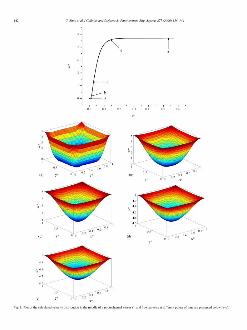
Fig. 8. Plot of the calculated velocity distribution in the middle of a microchannel versust* , and flow patterns at different points of time are presented below (a–e).

T. Zhou et al. / Colloids and Surfaces A: Physicochem. Eng. Aspects 277 (2006) 136–144 143

Fig. 9. The development of velocity inz-direction under different Reynoldsnumber.

by the pressure gradient, which is omitted in Yang and Hu’smodel [8,13]. They, hence, cannot observe the velocity basin,before the steady flow is set up. As the time goes, the velocityconsistent with the pressure profile is evolved, and there is alsoa slight downhill at the inlet and uphill at the outlet.

The velocity profiles in bulk at different time are presentedin Fig. 8. In this figure, we present velocity profiles in five timepoints in a 3D mode. From this presentation, how the steady flowis set up can be clearly figured out. InFig. 8,w∗ is thez-directioncomponent ofV* . Immediately after the external electric poten-tial is applied, the fluid on the wall of microchannel moved, andthen drives the bulk by viscous force. Since the time is veryshort, most of the bulk cannot be driven at once, they keep stillbecause of inertia. If we draw a figure to show thew∗ at thelateral section of microchannel, we can attain the results shownin Fig. 8a–e, which represents five different time points. We maystraightforward see that the velocity profile varies from bowl todish, and more and more close to the plane but it will never reach,because of the existence of the induced pressure. At time pointa (t* = 2.84× 10−3), velocity profile can be observed only nearthe channel wall (Fig. 8a); with the time goes, the velocity pro-files at the channel cross-section look like a bowl whose depthdecreases with the increase of time (Fig. 8b, t* = 1.42× 10−2; c,t* = 2.84× 10−2; d, t* = 0.142); At time beyond the time pointd (e.g., e,t* → ∞), the velocity profile changes from bowl- todish-like type, reaching a steady-state (Fig. 8e). If we neglectt lane.

3

V

R

T wec oldsns the

Fig. 10. The time that fluid needs to reach steady-state at different Reynoldsnumber by numerical simulation in 3D model.

Fig. 11. The time that fluid needs to reach steady-state at different Reynoldsnumber by analytical solution Eq.(29) in 1D model.

purpose of unification of unit of time, we setx-axis ast, insteadof t* , sincet* is a function ofRe. In the following calculation, wesetd = 15�m. FromFig. 9, we can find the laws that the smallerRe is, the faster the fluid will reach the steady state. We alsodefine that the fluid reaches steady state when velocity in thez-direction reaches 99% of its maximum.Fig. 10presents thetime that fluid needs to reach steady state in different Reynoldsnumbers by numerical simulation, whileFig. 11 presents thatby analytical solution Eq.(29). It can be seen that, to someextent, the trend inFig. 10is similar to the one inFig. 11. Thisbehavior can proof that 1D model is agreeable qualitatively with3D model. The omission ofy andz direction’s information leadsthe disparity between two models.

4. Concluding remarks

The characteristics of the electroosmotic flow in a directmicrochannel before it reaches the steady state have been stud-ied using analytical and numerical methods. The relationshipbetween Reynolds number and steady time was systematicallyexamined, and we obtained a conclusion that time required for

he induced pressure, the velocity profile will achieve the p

.3. Effect of Reynolds number on steady time

We have defined Reynolds number asρVsd/µ before, ands = εξEs/µ. So

e = εξρ(φout − φin)

µ2

o clarify the effect of Reynolds number on steady time,ompute several different problems with a range of Reynumbers and then plot the velocity distribution (Fig. 9) and theteady time (Fig. 10) as a function of Reynolds number. For

144 T. Zhou et al. / Colloids and Surfaces A: Physicochem. Eng. Aspects 277 (2006) 136–144

the fluid in microchannel to reach the steady state is very short ascompared to the one following mass transport of species needs.So the early unsteady flow upon application of voltage does notinfluence the later separation of samples. Also when perform-ing a theoretical analysis, instead of direct coupling method,we can use sequential coupling method to save computer timeand memory. Furthermore, induced pressure should be consid-ered since it may change the flow profile. Especially, at the inletand outlet of the microchannel, the pressure affects separationefficiency significantly. The results indicate that our model isan accurate and efficient simulation tool useful for designingoptimal electrophoretic separation microchips.

Acknowledgements

This work was supported by the Grants from the NationalNatural Science Foundation of China (Grant No. 20299033,20125515) and the Ministry of Education of China (No.20020284021).

References

[1] D.J. Harrison, A. Manz, Z.H. Fan, H. Luedi, H.M. Widmer, Capillaryelectrophoresis and sample injection systems integrated on a planar glasschip, Anal. Chem. 64 (1992) 1926–1932.

[2] A. Manz, D.J. Harrison, E.M.J. Verpoorte, et al., Planar chips tech-nology for miniaturisation and integration of separation techniques into

atogr

sey,997)

ma-alysis

ec-mpli-

ersehnol.

[7] R.J. Wang, J.Z. Lin, Z.H. Li, Analysis of electro-osmotic flow char-acteristics at joint of capillaries with step change in zeta-potential anddimension, Biomed. Microdevices 7 (2005) 131–135.

[8] N.A. Patankar, H.H. Hu, Numerical simulation of electroosmotic flow,Anal. Chem. 70 (1998) 1870–1881.

[9] E.B. Cummings, S.K. Griffiths, R.H. Nilson, P.H. Paul, Conditions forsimilitude between the fluid velocity and electric field in electroosmoticflow, Anal. Chem. 72 (2000) 2526–2532.

[10] U. Tallarek, E. Rapp, T. Scheenen, E. Bayer, H. Van As, Electroos-motic and pressure-driven flow in open and packed capillaries: velocitydistributions and fluid dispersion, Anal. Chem. 72 (2000) 2292–2301.

[11] A.E. Herr, J.I. Molho, J.G. Santiago, M.G. Mungal, T.W. Kenny, M.G.Garguilo, Electroosmotic capillary flow with nonuniform zeta potential,Anal. Chem. 72 (2000) 1053–1057.

[12] J.G. Santiago, Electroosmotic flows in microchannels with finite inertialand pressure forces, Anal. Chem. 73 (2001) 2353–2365.

[13] R.J. Yang, L.M. Fu, Y.C. Lin, Electroosmotic flow in microchannels, J.Colloid Interface Sci. 239 (2001) 98–105.

[14] P. Dutta, A. Beskok, Analytical solution of time periodic electroosmoticflows: Analogies to Stokes’ second problem, Anal. Chem. 73 (2001)5097–5102.

[15] Y.D. Hu, C. Werner, D.Q. Li, Electrokinetic transport through roughmicrochannels, Anal. Chem. 75 (2003) 5747–5758.

[16] G.Y. Tang, C. Yang, J.C. Chai, H.Q. Gong, Joule heating effect onelectroosmotic flow and mass species transport in a microcapillary, Int.J. Heat. Mass Transfer 47 (2004) 215–227.

[17] G.Y. Tang, C. Yang, C.J. Chai, H.Q. Gong, Modeling of electroos-motic flow and capillary electrophoresis with the joule heating effect:the Nernst–Planck equation versus the Boltzmann distribution, Langmuir19 (2003) 10975–10984.

[18] H. Matsumoto, N. Komatsubara, C. Kuroda, N. Tajima, E. Shinohara, H.icro-2004)

[ ns ofem.

[ per-003)

[ nce,

[ s ofnels,

monitoring systems, Capillary electrophoresis on a chip, J. Chrom593 (1992) 253–258.

[3] A.G. Hadd, D.E. Raymond, J.W. Halliwell, S.C. Jacobson, J.M. RamMicrochip device for performing enzyme assays, Anal. Chem. 69 (13407–3412.

[4] D.J. Harrison, K. Fluri, Z.H. Fan, C.S. Effenhauser, A. Manz, Microchining a miniaturized capillary electrophoresis-based chemical ansystem on a chip, Science 261 (1993) 895–897.

[5] T. Tang, M.Y. Badal, G. Ocvirk, et al., Integrated microfluidic eltrophoresis system for analysis of genetic materials using signal afication methods, Anal. Chem. 74 (2002) 725–733.

[6] R.J. Wang, J.Z. Lin, Z.H. Li, Study on the impacting factors of transvdiffusion in the micro-channels of T-sensors, J. Nanosci. Nanotec5 (2005) 1281–1286.

. Suzuki, Numerical simulation of temperature distribution inside mfabricated free flow electrophoresis module, Chem. Eng. J. 101 (347–356.

19] S.V. Ermakov, S.C. Jacobson, J.M. Ramsey, Computer simulatioelectrokinetic injection techniques in microfluidic devices, Anal. Ch72 (2000) 3512–3517.

20] E.K. Zholkovskij, J.H. Masliyah, J. Czarnecki, Electroosmotic dission in microchannels with a thin double layer, Anal. Chem. 75 (2901–909.

21] R.F. Probstein, Physicochemical Hydrodynamics, Wiley-Interscie1994.

22] Y.H. Zhang, X.J. Gu, R.W. Barber, D.R. Emerson, An analysiinduced pressure fields in electroosmotic flows through microchanJ. Colloid Interface Sci. 275 (2004) 670–678.