DI

SC

US

SI

ON

P

AP

ER

S

ER

IE

S

Forschungsinstitut zur Zukunft der ArbeitInstitute for the Study of Labor

Time Costs of Children as Parents’ Foregone Leisure

IZA DP No. 5760

June 2011

Olivia Ekert-JafféShoshana Grossbard

Time Costs of Children as Parents’ Foregone Leisure

Olivia Ekert-Jaffé Institut National d’Etudes Démographiques

Shoshana Grossbard

San Diego State University, University of Zaragoza and IZA

Discussion Paper No. 5760 June 2011

IZA

P.O. Box 7240 53072 Bonn

Germany

Phone: +49-228-3894-0 Fax: +49-228-3894-180

E-mail: iza@iza.org

Any opinions expressed here are those of the author(s) and not those of IZA. Research published in this series may include views on policy, but the institute itself takes no institutional policy positions. The Institute for the Study of Labor (IZA) in Bonn is a local and virtual international research center and a place of communication between science, politics and business. IZA is an independent nonprofit organization supported by Deutsche Post Foundation. The center is associated with the University of Bonn and offers a stimulating research environment through its international network, workshops and conferences, data service, project support, research visits and doctoral program. IZA engages in (i) original and internationally competitive research in all fields of labor economics, (ii) development of policy concepts, and (iii) dissemination of research results and concepts to the interested public. IZA Discussion Papers often represent preliminary work and are circulated to encourage discussion. Citation of such a paper should account for its provisional character. A revised version may be available directly from the author.

IZA Discussion Paper No. 5760 June 2011

ABSTRACT

Time Costs of Children as Parents’ Foregone Leisure* This article uses data from the 1998-1999 French INSEE time use survey to estimate the time costs of children. The focus is on couples with two spouses working Full-Time in the labor force in order to avoid issues of substitution between home production and labor supply. Time costs are computed in terms of hours of foregone leisure. The model accounts for selection into full-time employment and controls for use of hired childcare workers. We find that the foregone leisure cost of one child under age 3 is 1.9 hour for mothers and 2.2 hours for fathers. We find economies of scale for mothers but not for fathers. The presence of a childcare worker per child reduces the time cost of children to a couple of parents by 5%. JEL Classification: J13, J22 Keywords: children, time costs, leisure Corresponding author: Olivia Ekert-Jaffé INED 133 bd Davout 75980 Paris Cedex 20 France E-mail: ekert@ined.fr

* The authors thank UNAF and Christine Barnet-Verzat for help with the construction of the database. Thanks are also due to Noël Bonneuil, Robert Breunig, Elisabeth Cudeville, Dominique Meurs and participants at the ‘seminaire genre’ at the University of Paris 1 Pantheon-Sorbonne.

1. Introduction

That children involve a time cost has been recognized at least since

the work of Girard (1958), Becker (1960, 1965), and Mincer (1963).

Estimations of that time cost have focused on the opportunity cost of

children in terms of reduced parental working hours, and consequently,

loss of income. Examples of such estimations include Kravdal (1992),

Waldfogel (1998), Joshi et al. (1999), Gangl et al. (2009), Meurs et

al.(2010), and Bryan and Sevilla-Sanz (2011). The availability of time use

surveys makes it possible to calculate the time costs of children directly

by calculating the additional household production time associated with

the presence of children, as was done, for instance, by Gustafson (1994),

Sousa-Poza et al. (2001), and Gutierez-Domenech (2010). This way of

using time-use data to calculate the cost of children is problematic for at

least two reasons: (1) substitution between household production and

work in the labor force may provide parents with income to pay for hired

help, and (2) multitasking makes it difficult to identify household

production, including childcare (Sayer et al. 2004). Instead, we propose to

calculate the opportunity cost of children in terms of foregone leisure.

By reducing their labor supply parents can possibly devote time to

child care and other forms of home production without foregoing leisure.

As a result, foregone leisure time is a better measure of the opportunity

cost of children in couples with two fully employed parents—who

presumably don’t reduce their labor supply after a child is born--than in

couples in which one parent (typically the woman) switches to part-time

work or drops out of the labor force after a child’s birth. Consequently, we

2

base our calculations of foregone leisure on a comparison of the leisure

time of parents and childless adults after correcting for the selection bias

caused by the elimination of couples who don’t work full-time. In

contrast, studies such as Craig and Bittman (2008) that also estimate the

cost of children in terms of parental foregone leisure have included

women who do not work full-time in their sample and have not modelized

the decision to work full-time.

Our results, based on the French INSEE survey of 1998-1999, reveal

substantially lower parental leisure when children are present than when

they are not. Leisure is especially lower in the case of children under age

3. In a comparison with similar childless women we find that 1 child

under age 3 is associated with a loss of 1.9 hours of leisure per day, the

equivalent being a loss of 2.2 hours for men. These time costs of children

increase with family size and decrease as children grow older. We find

evidence of economies of scale for women but not for men.

We define leisure as including personal care (sleeping, eating and

grooming) as well as ‘pure leisure’ and show how children affect both

types of leisure for men and women. We demonstrate the importance of our

simultaneous estimation of leisure and full-time employment by comparing

our results with those that don’t address the problem of selectivity into full-

time employment.

The high time costs of children that we document are likely to

discourage fertility and exacerbate the aging of the population in

industrialized countries. We show that use of childcare workers

3

significantly reduces the time costs of children to parents. Our analysis can

help design optimal policies affecting fertility and labor supply.

2. Methodology

Our goal is to estimate French couples’ (1) foregone leisure

associated with the presence of children and (2) the monetary cost of

children using this foregone leisure as its base.

2.1 Foregone leisure

In line with Gronau (1973), Barnet-Verzat and Ekert-Jaffé (2003)

and Hamermesch (2009) leisure is defined as the time left after both

household production time and paid work--including commuting time--

have been deducted. Since we want to focus on substitution between home

production and leisure rather than between home production and labor

supply we compare the leisure time of parents and childless adults in

couples consisting of two partners working full-time (FT) in the labor force

and we exclude couples with mothers who work part-time or not at all.

However, since mothers who work FT differ systematically from mothers

who don’t work FT, we will be correcting for the bias that occurs when

selecting couples with two FT workers. The validity of foregone leisure as

a measure of the time cost of children depends not only on whether parents

make more childcare time available by reducing their hours in the labor

force. Parents can also maintain high levels of leisure by hiring childcare

workers. Therefore, ideally, we would want to limit our estimates not only

to couples with two fully employed parents but also to couples who don’t

4

employ any paid childcare workers. However, eliminating parents

employing childcare workers is not a valid option as it would leave us with

an exceedingly small sample. We take account of possible substitution

between parental care and paid childcare by controlling for the presence of

hired help in our leisure equations.

Leisure equations. We denote leisure by lf, and lm, where subscripts

f and m stand for ‘woman’ and ‘man’. Leisure is estimated according to the

following equation:

0 1 2 3 4 5 6 i(1) ln ln fi fi mi i i f ml f f w f w f N f Z f Z f Z u= + + + + + + +

where subscript i denotes the couple, wm and wf the hourly wages of

men and women and N is a vector indicating the number of children in

various age-groups. Our focus is on how the presence of children of

various age groups--but younger than 15--affect leisure, which implies that

we will be estimating a vector . We distinguish between children age 3

or younger and children older than 3.

f3

2 Vector includes the following

couple-level control variables: number of children ages 15 to 24 and

presence of hired help (such as paid childcare). Such help may help

alleviate the leisure loss associated with children. The more it is available,

the more parents are likely to engage in leisure.

Zi

Vector also includes married status. To the extent that common-

law couples are more egalitarian than married couples (Ekert-Jaffé and

Zi

2 We experimented with distinguishing between the 3-to-5 and the 6-to-14 age groups but did not find significant differences in the effects of children in these two age categories on parental leisure. Therefore we collapsed the age groups. We also experimented with setting the age limit at different ages and found that the time cost is null precisely after the age of 15.

5

Sofer 1996) we expect cohabiting women to obtain more leisure than

comparable married women. However, married women may have more

leisure than cohabiting women to the extent that marital status is an aspect

of higher benefits received by women in couple (see Grossbard-Shechtman

1993). Such benefits may include better access to material resources and/or

leisure. These two ‘effects’ of marital status may cancel each other and we

don’t have an unambiguous prediction regarding the effect of marital status

on women’s leisure.

Another variable included in is the difference between his age

and her age. We expect that difference to matter, for it indicates a woman’s

relative bargaining power. The higher this power relative to the man’s

power, the more a woman is likely to acquire leisure time in her couple.

This is a possible application of the concept of orchestration power

analyzed in economic models of intra-household allocation such as

McElroy and Horney (1981), Grossbard-Shechtman (1993) and Browning

et al (1994). We expect that women who are substantially younger than

their husbands or partners are more desirable in marriage markets (see

Becker 1973) and therefore able to obtain more leisure in their couple than

women who are not younger than their partners. Alternatively, older men

may be more authoritarian, in which case we expect that women who are

substantially younger than their husbands will have less access to leisure.

Zi

6

Finally, vector includes average age of the partners (a proxy for

age and cohort effects), type of residential area, time of year

Zi

3, day of the

week, and non-work income estimated as total income (by income bracket)

minus income from work using the method of the simulated residuals. 4

Personal characteristics that may be related to cost of time are

found in vectors of personal control variables and and include both

partners’ occupational status (self-employed versus employed) and

educational level.

Zf Zm

Accounting for selection bias. We need to account for the fact that

we estimate foregone leisure on the basis of a sample from which mothers

who are working part time and women out-of-the-labor-force have been

eliminated. Those who continue to work are likely to be very devoted to

their work, to have made special arrangements for their children’s day-

care, or not to have the choice of stopping work due to their need for

income. Many women with substantial family demands on their time stop

working full-time and may be missing from a sample of full-time women

workers. We therefore also estimate the decision to work full-time (FT) as

part of two systems of two equations: (1) women’s leisure and their FT

employment ratio and (2) men’s leisure and their partner’s FT employment

ratio.

3 ‘Spring/summer’ was defined as the period between15 February and 27 September 1998 while ‘Winter’ was defined as the period from September 27, 1998 to February 14, 1999. Otherwise there were no systematic month-to-month differences. 4 These estimates control for socio-occupational categories and housing status (renter/owner with mortgage, full owner).

7

Our indicator of FT employment in the labor force (LF) is y, a

woman’s FT employment ratio or the proportion of time a woman spends

in FT employment. It is defined as usual hours of work in the LF divided

by hours corresponding to full-time work.5 It takes values between 0 and 1:

y = 1 means that the woman in the couple is employed full-time and y = 0

that she is out of labor force.

FT employment is modeled as:

(2) i i iy Yγ η ε= + +

where Y is a vector of explanatory variables that differs from Z in

equation 1. It includes number of children in three age groups: 0-2, 3-to-5

and 6 to 14.

Then we estimate two equations simultaneously: leisure of the

woman (or the man) and the woman’s FT employment ratio.6 The

dependent variables become latent variables lf,i*, lm,i* and yi*, resulting in

the following two-equation systems. The first system is for the woman’s

leisure and her FT employment ratio:

0 1 2 3 4 5 6 i(3 ) * ln ln fi fi mi i i f ma l f f w f w f N f Z f Z f Z u= + + + + + + +

(3 ) * ; i i ib y Yγ η ε= + +

5In 1998 the French government defined a full-time job as one that involves a minimum of 39 hours a week. On average this amounts to 5.5 hours per day when we take weekends and holidays into account. 6 We also tried to estimate a system of three simultaneous equations: leisure of both men and women in couples and women’s full-time (FT) employment ratio. However, such model did not converge.

8

Similarly, we estimate an equation system (4a, 3b) for man’s leisure

and woman’s FT employment ratio:

0 1 2 3 4 5 6 i(4 ) * ln ln mi fi mi i i f ma l f f w f w f N f Z f Z f Z u= + + + + + + +(3 ) * ; i i ib y Yγ η ε= + +

For models (3a; 3b) and (4a; 3b) to be identified, Y in equation 3b

must contain an instrument that explains women’s FT employment ratio yi

without affecting leisure lf (lm) or wage. This instrument is the local

unemployment rate, which proved to be a good instrument (exogenous with

respect to leisure and correlated to labor force participation).

Estimated Wages. Equations 3a and 3b include the wage of each

partner. However, low wages may be the result of low investments in work

and high levels of leisure. We address this endogeneity problem by

constructing exogenous wages that are assumed to influence time use

without the possibility of reverse causality:

(5)ln * jiw α= + ijX ,β + ij,ν ; mfj ,=

We then replace actual wages w with w* in equations 3a and 3b. As

instruments in the estimated wage equations we use socio-occupational

categories for we found that they influence wages but not leisure. Vector X

also includes detailed educational level, age and age squared (see Mincer

1974).

The two equation systems, including leisure time of either the wife or the

husband and the wife’s full-time employment ratio, are estimated with a

bivariate Tobit model (see Heckman 1979, Lee and al. 1980 and Lollivier

2002 and 2006). Women’s FT employment ratio is estimated from a

9

sample of 2,447 households, including women who work part-time or are

out of the labor force. Leisure equations are estimated for a sample of

1,148 couples that only includes couples in which women working full-

time. All standard deviations and tests are obtained by bootstrapping (see

Horowicz 2004).

2.2 Time cost of children in monetary terms

Ever since Mincer (1963) and Becker (1965) it has become

customary to translate time costs into monetary terms by multiplying the

time it takes individuals to do something with their value of time. If the

individuals are in the labor force—as is the case with all the respondents in

our sample--their value of time is their wage.

Translating the time cost of children into monetary values can be

done at the individual or the couple level. Doing so at the couple level is

more consistent with unitary levels of decision-making that consider the

couple as the decision-making unit and in which couples make decisions

based on their combined resources. In contrast, in non-unitary models

individual members of couples or other multi-person households have their

own preferences and control over their own resources. Such non-unitary

models have been applied to labor supply (e.g. Grossbard-Shechtman and

Neuman 1988, Chiappori, Fortin and Lacroix 2002), consumption (e.g.

Thomas 1990, Browning et al. 1994, and Lundberg, Pollak and Wales

1997), and, more recently, to the cost of children (e.g. Blundell et al. 2005

and Picard and Matteazzi 2010).

For our purpose--to translate foregone leisure into monetary

terms—we take a simple approach to calculating costs of children at the

10

individual level: we assume that individual men and women continue to

make their own decisions and to be influenced by their own income even

when married. The monetary cost of children based on foregone leisure is

equal to value of leisure divided simply c, leisure time divided by T (let us

say 24 hours):

(6 ) / /fi fi fi fi fia c w l w T l T= =

(6 ) / /mi mi mi mi mib c w l w T l T= =

where T stands for total hours. This variable is defined for an

individual woman f and a man m in a couple i and gives the monetary value

of foregone leisure relative to personal full income. To the extent that

rational individuals make decisions on their own—rather than as couples--

these costs are also the ones that they will take into account when deciding

on fertility, consumption, or labor supply.

In addition, we also calculate the time cost of children using the

couple as the decision-making unit. The cost variable that we focus on is

based on Kooreman and Kapteyn’s (1987) first method 7 for estimating the

time costs of two-earner couples and is defined as

(7) . ( ) / (i fi fi mi mi fi mic w l w l w w= + + )T

Specifically, we multiply a person’s leisure time with that person’s

wage to get an individual’s value of leisure. We then add both partners’

value of leisure and divide that total value of leisure by the couple’s full

7 A second method in Kooreman and Kapteyn (1987) includes couples with stay-home women. Our method differs from theirs in that we only select couples with two spouses working FT and that we aggregate all leisure activities, whereas they examined separate time uses.

11

income. This cost variable captures the value of foregone leisure as a

proportion of couples’ full income. It makes sense as public policies are

often considered at couples’ level. It makes sense to the extent that couples

consider costs and benefits of having children as part of a couple’s

decision. When Kooreman and Kapteyn divide by the couple’s full

income, they follow Becker’s (1965) unitary approach that assumes

implicitly that all incomes are pooled into a household income.

To calculate couples’ monetary value of foregone leisure we re-

estimate the same equations presented above for leisure time but replace

leisure time with the cost variable in equation 7.

0 1 2 3 4 5 6 i(8) * ln ln i fi mi i i f mc g g w g w g N g Z g Z g Z u= + + + + + + +

(3 ) * , i i ib y Yγ η ε= + +

where y* is the woman’s FT employment ratio defined above.

3. Data

We use the time use survey carried out in France by INSEE in 1998

and 1999. The information was collected in diaries in which the

respondents noted the duration of their activities during the day. In order to

allow for variations in activities over the week, the sample contained

roughly the same number of diaries for each day of the week. Seasonal

variations were also considered, the survey having been administered in 8

waves from February 16, 1998 to February 14, 1999 (omitting the August

holiday period).

12

We selected couples in which each spouse filled in at least one time

use diary and in which men were younger than 60 and were employed full-

time. We also eliminated 292 questionnaires containing missing values and

another 48 couples for whom estimated wages diverged from the observed

wages by more than 30%.

Table 1 presents descriptive statistics for the 2,447 couples included

in our analyses. It can be seen that women were working full-time in 49%

of the couples. The other couples were divided equally between couples

with women working part-time and couples with women out of the labor

force. Couples with two full-time partners have one child on average. Of

these couples 12% have at least one child under 3. In contrast, couples with

women who don’t work FT have almost 2 children on average. They are

also more likely to have a child under age 3 than couples with two FT

earners. Table 1 indicates the direction of the bias involved in selecting

women employed full-time: there are more large families among women

out of the labor force or working part-time than among women working

full-time. Women may spend more time on domestic work rather than

being in FT employment because they have more children or because they

are more traditional. More time in home production may also be associated

with lower wage in the labor market. We therefore try to control for these

variables.

Table 1 also shows that hours of leisure of both men and women

vary with women’s labor status and family size. On average, women out of

the labor force have more leisure than women in the labor force. Men

13

married to women out of the labor force also have more leisure than men in

couple with a FT worker.

Larger family size tends to be associated with less leisure, but there

are exceptions judging from Table 1. The most leisure is observed for

women out of the labor force without children under 15. For this group it

appears that the presence of children age 14 or younger is clearly

associated with loss of leisure. However, women working part-time don’t

appear to experience a loss of leisure when they have one child, even if the

child is under 3. These large differences between women who work FT and

those who don’t add to the validity of our decision to limit the analysis to

couples with two FT workers. The following econometric analysis offers a

more precise measurement of the leisure that workers employed in the LF

forego when having children.

4. Results

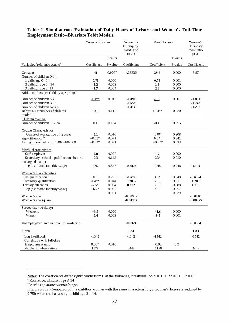
Table 2 reports estimations of the two equation systems including

individual leisure and woman’s FT employment ratio. Columns 1 and 2

present woman’s leisure and employment ratio (equations 3a and 3b) and

Columns 3 and 4 report estimations of man’s leisure and woman’s

employment ratio (equations 4a and 3b). Leisure is measured in daily

hours.

A first step is to calculate the amount of leisure time available to

representative men and women without children under age 14 (i.e. childless

adults). Based on the constant terms in columns 1 and 3, the coefficients

14

indicating the effects of the control variables on leisure, and mean values

for these variables, we calculate the hours of daily leisure for representative

couples with a woman who works FT in the labor force.8 As reported in

Table 3, childless representative men and women each have 13.5 leisure

hours. On weekends men’s leisure increases more than women’s:

representative childless women have 17 hours of leisure and representative

childless men have 18.1 hours.

A second step is to use the coefficients of number and age of

children reported in Table 2 (columns 1 and 3) to assess leisure foregone

due to the presence of children. The corresponding leisure losses and daily

hours of leisure for representative men and women with children are

reported in Table 3 (cols 1 and 2 for women; cols 4 and 5 for men). The

time cost of children varies with their age and family size. On an average

day of the week the presence of one child age 0-14 reduces a woman’s

leisure time by .75 hour and a man’s leisure time by .73 hour, leaving

women with 12.7 leisure hours and men with 12.8 leisure hours on

weekdays. The leisure loss associated with the presence of a child under 3

is considerably higher than that of a child age 3-14: the extra cost of a child

under age 3 is 1.1 hours for mothers and 1.5 hours for fathers. The total

loss of leisure time associated with the presence of one child under 3 is

obtained by adding the coefficient of one child age 0 to 14 and one child

under 3 and for a woman equals 1.87. Accordingly, the representative

8 This is calculated as follows: if the woman in a reference couple is 38.5 years old and has a monthly wage of 8,867 (Log=9.09) 1998 FRF and the 40.9 years old man earns 11,175 (Log=9.32) 1998 FRF, the woman has (-0.02 x 9.32 + 6.6 x 9.09 –0.1x39.9 + 0.05x2.04 - 41)=13.5 hours of leisure on a weekday.

15

woman is left with 11.6 leisure hours per day. Men in these circumstances

have almost the same leisure.

The time costs that we have estimated are large. We have

confirmed what was stated by economists Wachter and Willis (1973) and

Becker (1991): young children are primary consumers of their parents’

time. In contrast, the time cost of children ages 15 to 24 is zero. That the

presence of older children is not associated with a statistically significant

loss of leisure could possibly be the result of older children taking care of

younger children (see Sousa-Poza et al. 2001) or of the fact that older

children consume less of their parents’ time.

Next, we look at how number of children ages 3-14 affects their

parents’ leisure. Comparing the impact of two children age 3-14 to the

impact of one child in that age range, we find that the loss of leisure

increases from .75 to 1.2 hours for women and from .73 to 1.6 hours for

men. The loss of leisure experienced by men with two children is thus

about twice that of men with one child in this age range, but for women it

is less than twice the loss experienced with one child. This implies the

presence of economies of scale for mothers but not for fathers. As for three

children ages 3 to 14, they reduce mothers’ leisure by 1.7 hours and

fathers’ by 2.2 hours. Again, we find more foregone leisure for fathers than

for mothers. Relative to the time cost of one child, mothers of two children

spend 40% less time per child, and mothers of three children spend 33%

less per child. We also see that when there are 2 children under age 3,

leisure is reduced to 10 hours for women and 8.9 hours for men. With 3

children, including one under age 3, leisure time goes down to 10.4 hours

16

for women and 9.8 hours for men. Given that men have 1.1 hour of leisure

more than women on a weekend day, overall—for any day of the week

including weekends--mothers and fathers of three children have about the

same amount of leisure. Parents have little leisure left if they work full-

time, especially if their children are young and they can only afford

childcare supplied by the state (Fagnani and Math 2011).

Our results indicate that on weekdays the cost of children is not

lower for men than for women. However, our model is based on one

period—the present. In fact, from a life-cycle perspective men may not

experience higher time costs than women, for they give up leisure to work

more in the LF and thereby accumulate experience (which leads to higher

wages) and pension benefits which is not the case with women who reduce

their hours of work in the LF after children are born (see Pailhe and Solaz

2006, Meurs, Pailhé and Ponthieux 2010). Even if this gender difference

mostly reflects men’s increased hours of paid work after the birth of

children, the cliché of fathers watching television while their wives take

care of the children and cook dinner does not apply to most French couples

in our sample.

That we find economies of scale for women but not for men could

be related to increased gender-based specialization among couples with

more children: men tend to work more in the labor force and women more

at home (see Brousse 1999; Anxo et al 2002). Consequently, if there are

economies of scale in meal preparation and in childcare, this will save

mothers’ time more than fathers’. Men have fewer opportunities to utilize

time-saving economies of scale related to number of children. Our

17

selection of couples with two spouses working full-time does not preclude

gender-based specialization: men appear to work longer hours in the labor

market than women, and more so when there are more children. They are

likely to take jobs with a longer commute or work more overtime. In fact,

we find that in our sample of full-time dual earners men work on average

6.3 hours in the labor market and women 5.4 hours. This climbs to 7.3

hours for fathers of 2 children with one child under 3 whereas mothers of

children that age work 1.7 hours less in the LF than women without

children.

What aspects of leisure are most likely to be cut? The way we

define leisure, it includes all the time they have for personal care, including

sleeping and eating, as well as for ‘pure leisure’ (defined as leisure other

than sleeping, eating and other forms of personal care) on an average

weekday. As can be seen in Table 4 loss of leisure time for women

associated with the presence of one child consists equally of lost pure

leisure and lost personal care. In contrast, men’s pure leisure is unaffected

by the presence of one child age 3-14 but younger children or larger

families reduce fathers’ hours of sleep as well as mothers’. Having three

children age 3-14 “costs” the mother and the father a little less than one

hour of personal care each; the corresponding figure for a young child is

around one hour for each parent.

Relative costs of children

Costs of children relative to full income were computed for both

individuals and couples. For individual men and women hours of foregone

leisure, expressed as a percentage of 24 hours, amount to the cost of

18

children to the individual as a proportion of their personal full income.

Columns 3 and 6 in Table 3 present the relative leisure costs of women and

men. For instance, child younger than 3 leads to a leisure loss valued at

7.8% (9.2%) of a woman’s (man’s) full income. These are large leisure

losses relative to the average hours that defined full-time employment in

France at that time: 5.5 hours a day, which is 22.9% of T.

For couples, we estimated regressions of the time cost of children

as a function of the couple’s full income according to equations 3b, 7, and

8. The results are reported in Column 7 of Table 3. It can be seen that a

representative couple with one child age 3-14 experiences a time cost that

amounts to 3% of its full income. In other words, a child reduces the

couple’s full income by 3%. This calculation takes account of the fact that

an hour of an uneducated person has less value than an hour of a highly

educated person and allows for substitution between father’s time and

mother’s time in household production. Table 3 also reports the relative

time cost of more children and children of different ages. For instance, it

can be seen that a child under age 3 costs a couple 8.2% of their full

income. The relative costs of children to couples, estimated with our two-

equations model, appear to be somewhere in-between the relative costs of

women and of women (based on a comparison of columns 3, 6, and 7 in

Table 3).

It would be interesting to compare these relative time costs of

children to the scale set by the OECD to calculate the monetary costs of a

child under 14 as fraction of the earnings of a representative childless

couple. These relative costs in France amounted to 20% of such earnings in

19

the case of children under age 14 and to 33% if the child is older than 14

(Hourriez and Olier 1998). We just note that—not surprisingly—time costs

are highest when children are under age 3 whereas monetary costs peak

when the children are older than 14.

In our estimations we took account of the fact that some couples

hire childcare workers so they can have more leisure: we controlled for the

presence of a childcare worker (such as baby-sitter) in our regressions.

Therefore our results are for parents not using childcare workers. Table 5

also shows how the presence of a childcare worker alleviates the time cost

of children in terms of actual foregone leisure: per child it reduces the

relative leisure loss to a couple by 5% of its full income.

Findings regarding other variables. Table 2 also shows that women

in older couples (using the average age in the couple) have less free time (7

minutes less for each additional year), in part because they work longer

hours in the LF. In contrast, men’s leisure is not affected significantly by

age. Age may affect women’s leisure more than men’s to the extent that

norms regarding household work by women have become less popular (see

Sevilla-Sanz and Gimenez 2011). Women’s leisure time rises slightly with

the age gap between spouses (by 3 minutes per additional year), which

supports the argument made above: youth may be an asset for women in

marriage markets and they may translate this advantage into having their

partner agree to their own higher level of leisure in their household.

Table 2 also reveals that leisure time does not depend on couples’

legal status but is affected by the season (half an hour a day less for each

spouse in winter) and the day of the week (on weekends men have 4.5 extra

20

hours of leisure and women 3.5 extra hours). Gender inequality is large on

weekends: women work one hour more than their partners. Leisure time

also depends on the city size: in urban areas of 20,000 to 100,000

inhabitants both men and women have extra leisure. This may reflect the

higher quality of life in mid-sized provincial towns (Bruno 1998). Self-

employed men—which includes farmers—have longer than average

working days, and consequently less leisure time (–1.6 hour per day). The

same is true for their spouses, but only by half as much (–45 minutes per

day). The table does not include non-work income, as the variable had no

significant effect on leisure.

We find an interesting contrast in the effect of education and wages

for men and women. For men, own educational level or estimated wage

have no effect on leisure time.9 In contrast, both own education and wages

influence women’s leisure time: at higher educational levels women have

less leisure. This is consistent with education being associated with high

expectations concerning quality of home life and children’s quality. It is

also well-documented that mother’s education is positively associated with

children’s quality (Leibowitz 1975). Controlling for educational level and

labor market participation, women’s wage appears to have a positive

influence on their leisure time.10 This may reflect an income effect: higher

income makes it possible to eat out more, use more cleaning services, etc.,

9 At first actual (and not estimated) wage was included in the estimation. We found what appeared to be a negative influence of observed wage on leisure, but this was probably a reverse effect: those more involved in their work have both less leisure time and higher wages. After control for such past investment in work by estimating wages according to Mincer (1974) it appeared that a man’s hourly wage rate does not influence his leisure. 10 It should be kept in mind that these are women who already have a full-time job and our model includes a full-time employment equation.

21

and thus to reduce time spent on domestic tasks. Fully employed women

earning higher wages may also have higher productivity in both work in

the LF and work in home production (see Grossbard-Shechtman 1993),

which could also add to their leisure time.

Cross-wage and cross-education effects on foregone leisure were

not found to be significant. We also checked for interactions between these

main determinants of leisure time and presence and number of children and

found no evidence for such interactions. In contrast, monetary costs of

children depend on income and socio-demographic characteristics (Ekert-

Jaffé and Trognon, 1994)

Sensitivity of the results to the selection of couples with two Full-

Time earners. Our results are influenced by the inclusion of a full-time

employment equation that addresses the problem of selectivity into full-

time work. To demonstrate the extent of the sample selection bias we also

estimated leisure time simultaneously for fathers and mothers working full-

time without considering women’s selection into full-time work. These

results (Ekert-Jaffé, 2010, table 3) indicate that when such selection is not

taken into account foregone leisure for children under 3 is about half of

what we report in our tables.

Our estimates of the effects of young children on foregone leisure

are larger than those found by Craig and Bittman (2008) using Australian

data. They estimated the time costs of one child age 0-2 in 1997 at 0.3

hours for fathers and 1.4 hours for mothers, in contrast to our estimate of,

respectively, 2.2 and 1.9 hours. Their estimate of the effect of three

children age 3-11 on fathers (a leisure loss of 0.8 hour) is also smaller than

22

our estimate of a 1.7 hour loss for three children aged 3-14, but our results

for mothers of 3 older children and for parents with one older child are the

same.

The differences between our time cost estimates and those of others

can be attributed to our focus on fully employed workers and our control

for selectivity in FT employment. We get larger negative effects of young

children on parental leisure because (a) we only look at couples working

FT and have eliminated what is possibly a positive effect: individuals with

more children are expected to work less in the labor force, possibly leading

to a positive association between children and leisure and reducing the

coefficient of ‘children’ in leisure time equations that don’t restrict the

sample to couples in full-time employment; and (b) we control for

selectivity bias and individuals who stopped working FT in the labor force

after a child’s birth may have had higher time cost if they had remained in

FT work . This reasoning also helps explain why our results are similar to

those of Craig and Bittman in the case of older children, for in that case the

causality ‘children full-time employment’ is less relevant (most mothers

are in the labor force) and less is lost by not taking account of a selectivity

bias.

By taking account of selectivity into full-time employment we also

get different results regarding the association between women’s education

and hours of leisure. We found that more educated women have less

leisure, as shown in Table 2. In contrast, there is no effect of education or

of wages when we do not take selectivity into account (Ekert-Jaffé 2010).

It is possible that women who do not like housework simultaneously have

23

more leisure time and invest more in their education and profession,

leading to a positive observed association between leisure time and

education. Our model eliminates such alternative causality and therefore

the negative causal effect that goes from education to leisure can be

identified. Likewise, by not making FT employment endogeneous a simple

model picks up reverse causality between wages and leisure: greater past

and present involvement in professional work (and choice of a less

leisurely lifestyle) generates higher wages, implying a negative association

between wage and leisure. This reverse effect disappears if the propensity

to work FT is part of the model and this helps explain why we find a

statistically significant positive association between wage and leisure.11

Our figures may be either under-estimates or over-estimates. They

may be underestimates for two reasons: (1) family meals and trips out with

the children have been counted as part of personal care and therefore as

leisure; and yet to some degree these activities are forms of household

production and could have been counted as ‘work’, and (2) we do not take

into account possible cuts in overtime hours or reductions in other forms of

household work. On the other hand, our figures might be over-estimates,

since we don’t rely on panel data and assume interpersonal comparability

of utility. More specifically, we assume that childless couples and those

with children have the same preferences for leisure. This assumption seems

to be justified to the extent that we find that when all their children are over

14 parents’ leisure time is equal to that of childless couples. However, to

11 Using the American Time Use data and not selecting full-time workers, Connelly and Kimmel (2009) found no significant association between relative wage and leisure time of parents.

24

the extent that people who became parents took less leisure time than

others even before they had children, what we interpret as the effect of

children would merely express different preferences.

5. Conclusion

This paper presented a unique methodology for calculating the time

cost of children in terms of foregone leisure. It is based on limiting the

analysis to men and women who work full-time in the labor force and

correcting for the selection bias caused by the elimination of couples who

don’t work full-time. Applying the method to a French time use survey

yielded time costs of children to mothers and fathers.

The results reveal substantially lower parental leisure when children

are present than when they are not. Leisure is especially lower in the case

of children under age 3. In a comparison with similar childless women we

find that the presence of 1 child under age 3 is associated with a loss of 1.9

hours of daily leisure for women and of 2.2 hours for men. These time

costs of children increase with family size. We find evidence of economies

of scale for women but not for men. Our results obtained for couples with

two full-time earners are simulating the behavior of all type of couples if

they would be in full time employment (Lee et al., 1980).

We discuss the direction in which estimates would be biased had

we not included corrections for selectivity bias. We compare our results to

estimates of foregone leisure associated with children without control for

selectivity and find support for our analysis. We hope that future work will

25

expand on this paper by using panel data that can help reveal unobserved

heterogeneity related to household composition. We estimated leisure and

selection into full-time employment separately for men and women.

Further work and better data may also permit simultaneous estimation of

the opportunity cost of children based on two leisure equations for man and

woman—as done e.g. by Bloemen and Stancanelli (2008)--as well as

selection of women into full-time employment,.

From a policy perspective the high time costs of children that we

document help explain why (1) parents—mothers in particular--often stop

working full-time when they have children and (2) fertility is so low in

industrialized countries. Many Western nations have instituted family-

friendly policies that lower the time cost of young children and have

simultaneously facilitated mothers’ return to work and encouraged fertility

(Datta Gupta et al 2008). For example, relative to other industrialized

nations, Sweden and France have relatively generous family-friendly

policies, high employment rates for mothers, and relatively high fertility.

A useful direction for furthering the research presented here is to

estimate foregone parental leisure in a number of countries differing in the

generosity and type of family-friendly policies. Such research could help

design optimal policies. Our findings also have implications for differential

treatment of parents and non-parents in retirement benefits such as

pensions and Social Security (see Burgraff 1998 and Cremer, Gahvari and

Pestieau 2008). Furthermore, to the extent that policies are aimed at

encouraging fertility, it may be necessary to target some policy tools to

26

men (Blundell et al. 2005) given that our research indicates that men’s time

costs of children are at the least as high as those of women.

References

Anxo, D., Flood, L. and Kocoglu, Y. (2002). Offre de travail et répartition des activités domestiques et parentales au sein du couple : une comparaison entre la France et la Suède. Economie et Statistique, 352-353 : 127-150.

Barnet-Verzat, C. and Ekert-Jaffé, O. (2003). Le coût du temps consacré aux enfants. Communication aux Journées de Micro-économie Appliquée, Montpellier, 5-6 juin.

Becker, G.S. (1960). An economic analysis of fertility. In Demographic and economic change in developed countries, a Conference of The Universities--National Bureau Committee for Economic Research. Princeton, N.J.: Princeton university press.

Becker, G.S. (1965). A theory of the allocation of time. Journal of Political Economy, 75: 493-517.

Becker, G.S. (1973). A theory of marriage: Part I. Journal of Political Economy, 81:813-846.

Becker, G. S. (1991). A treatise on the family. Cambridge, MA: Harvard university press.

Bloemen, H.G. and Stancanelli, E.G.F. (2008). How Do Parents allocate time? The effects of wages and income. Documents de Travail de l’OFCE, 2008-30.

Blundell, R., Chiappori, P.A. and Meghir, C. (2005). Collective labour supply with children. Journal of Political Economy, 113: 6.

Brousse, C. (1999). La répartition du travail domestique entre conjoints, permanences et evolutions entre 1986 et 1999 in France. Portrait Social, Insee : 135-151.

Browning, M., Bourguignon, F, Chiappori, P.A. and Lechene, V. (1994). Income and outcomes: A structural model of intrahousehold allocation. Journal of Political Economy, 102: 1067-1096.

Bryan, M.L. and Sevilla-Sanz, A. (2011). Does housework lower wages? Evidence for Britain. Oxford Economic Papers, 63 (1): 187-210.

Burggraf, S. (1998). The feminine economy and economic man, New York: Basic Books, 1998.

Chiappori, P.A, Fortin, B. and Lacroix, G. (2002). Marriage, market, divorce legislation, and household labor supply. Journal of Political Economy, 110 (February): 37-72.

Connelly, R. and Kimmel, J. (2010). Spousal influences on parents’ non-market time choices. Review of Economics of the Household, 7(4): 361-394.

27

Craig, L. and Bittman, M. (2008), The incremental time costs of children: an analysis of children’s impact on adult time use in Australia. Feminist Economics, 14(2): 59–88.

Cremer, H., Gahvari, F. and Pestieau, P. (2008). Pensions with pensions with heterogenous individuals and endogenous fertility. Journal of Population Economics, 21: 961-981.

Datta Gupta, N., Smith, and Verner, M. (2008). The impact of nordic countries’ family friendly policies on employment, wages, and children. Review of Economics of the Household, 6(1): 65-89.

Ekert-Jaffé, O. (2010). Le coût du temps consacré à l’enfant : contraintes de temps et activité féminine. Document de Travail INED, 163 : 48p.

Ekert-Jaffé, O. and Sofer, C. (1996). Formal versus informal marriage : explaining factors. in Evolution or Revolution in European Population, EAPS, 2: 65-85.

Ekert-Jaffé, O. and Trognon, A. (1994). Evolution du coût de l’enfant avec le revenu : une méthode. In Standards of Living an Families : 0bservation and Analysis, O. Ekert-Jaffé (ed.), Congrès et Colloques, 14, John Libbey et INED, Paris : 135-164.

Fagnani, J. and Math, A. (2011). France: gender equality, a pipe dream? in S. Kamerman, P. Moss (eds.), The Politics of Parental leave Policies, London, New-York, Policy Press : 103-118.

Gangl, M. and Ziefle, A. (2009.) Motherhood, labor force behavior and women’s careers: An empirical assessment of the wage penalty for motherhood in Britain, Germany and the United States. Demography, 46 (2): 341-369.

Girard, A. (1958). Le budget-temps de la femme mariée dans les agglomérations urbaines. Population, 4: 591-618

Gronau, R. (1973). The intrafamily allocation of time: the value of housewives' time. American Economic Review, 63: 643-51.

Grossbard-Shechtman, S.A. (1993). On the Economics of Marriage - A Theory of Marriage, Labor and Divorce. Boulder, Co: Westview Press.

Grossbard-Shechtman, S.A. and Neuman, S. (1988). Labor supply and marital choice. Journal of Political Economy, 96: 1294-1302.

Guillot, O. (2002). Une analyse du recours aux services de garde d’enfants. Economie et Statistiques, 352-353: 213-230.

Gustafsson, B. and Kjulin, U. (1994). Time use in child care and housework and the total cost of children. Journal of Population Economics, 7: 287-300.

Gutierrez-Domenech, M. (2010). Parental employment and time with children in Spain. Review of Economics of the Household, 8(3): 371-392.

Heckman, J.J. (1979). Sample selection bias as a specification error. Econometrica, 47 : 153-61.

Horowitz, J.L. (2001). The bootstrap. in: J.J. Heckman & E.E. Leamer (eds.), Handbook of Econometrics, 5: 3159-3228 Elsevier.

28

Hourriez, J.M. et Olier, L. (1998). Niveau de vie et taille du ménage : estimation d’une échelle d’équivalence. Economie et Statistique, 308/310: 65-85.

Kooreman, P. and Kapteyn, A. (1987). A disaggregated analysis of the allocation of time within the household. Journal of Political Economy, 95(2): 223-249.

Kravdal, O. (1992). Forgone labor participation and earning due to childbearing among norwegian women. Demography, 29(4): 545-563.

Lee, L.F., Maddala, G.S .and Trost, R.P. (1980). Asympotic covariance matrices of two stage probit or two stage tobit methods for simultaneous equations models with selectivity. Economica, 48: 491-503.

Leibowitz A. (1975). Education and the allocation of women's time. in F. T. Juster (ed.), Education, Income, and Human Behavior. New York : McGraw-Hill, 171-197.

Lollivier, S. (2002). Endogénéité dans un système d’équations normal bivarié avec variables qualitatives. Insee-Méthodes : Actes des Journées de Méthodologie statistique.12p.

Lollivier, S. (2006). Econométrie avancée des variables qualitatives, Economica, Paris.

Lundberg, S., Pollak, R.A. and Wales, T. (1997). Do husbands and wives pool their resources. Journal of Human resources, 32(3): 463-480.

Maddala, G.S. (1983). Limited dependent and qualitative variables in econometrics. Cambridge: Cambridge University Press.

Maresca, B. (1998). Les villes de 100 000 à 200 000 habitants peuvent devenir les plus attractives. Consommation et Modes de vie, 131 : 4p.

McElroy, M.B. and. Horney, M.J.(1981). Nash bargained household decisions: toward a generalization of the theory of demand. International Economic Review, 22: 333-49.

Meurs D., Pailhé A. and Ponthieux S. (2011). Child-related career interruptions and the gender wage gap in France. Annales d’économie et de Statistique, 99 ( forthcoming)

Mincer, J. (1963). Market prices, opportunity cost and income effects. in Measurement in Economics, C. Christ and al. eds. Stanford, CA: Stanford University Press.

Mincer, J. (1974). Schooling, Experience and Earnings. New York: Columbia University Press.

Pailhé, A. and Solaz A. (2006). Vie professionnelle et naissance. Population et Société, 426,.4p.

Picard, N. and Matteazzi,E. (2010). Collective model with children: public good and household production,. a conference “Economie de la famille”, INED, 18mars, 36p.

Sayer, L.C., Gauthier, A.H., and Furstenberg, F.F. (2004). Educational differences in parents’ time with children: Cross-national variations. Journal of Marriage and Family, 66 (December): 1149–1166.

29

Sevilla-Sanz, A. and Gimenez, J.I. (2010). Trends in time allocation: a cross-country analysis. Discussion paper 547, Department of Economics, Oxford University (April).

Sousa-Poza, A., Schmid, H. and Widmer, R. (2001). The allocation and value of time assigned to housework and child-care: an analysis for Switzerland. Journal of Population Economics, 14: 599-618.

Thomas, D. (1990). Intra-household resource allocation: an inferential approach. Journal of Human Resources, 25(4): 635-664.

Waldfogel, J. (1998). Understanding the “family gap” in pay for women with children. Journal of Economic Perspectives, 12(1): 137-56.

Willis, R. (1973) A new approach to the economic theory of fertility behavior. Journal of Political Economy, 81: S14-S64.

30

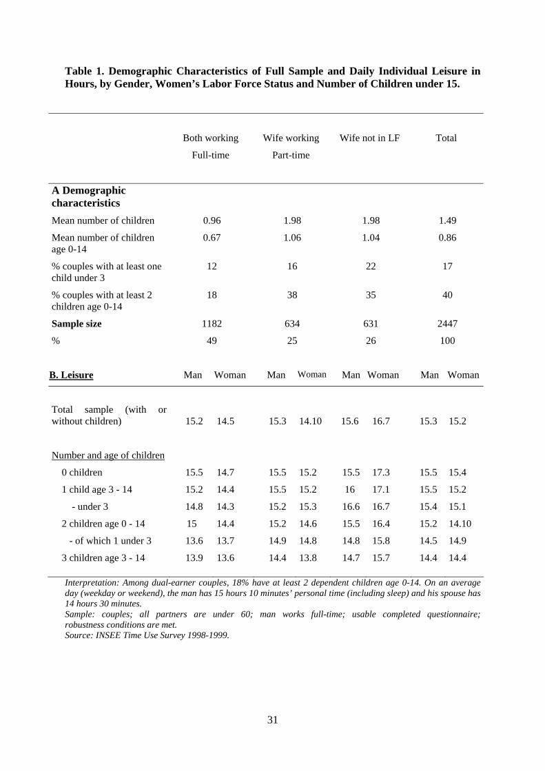
Table 1. Demographic Characteristics of Full Sample and Daily Individual Leisure in Hours, by Gender, Women’s Labor Force Status and Number of Children under 15.

Both working Wife working Wife not in LF Total

Full-time Part-time

A Demographic characteristics

Mean number of children 0.96 1.98 1.98 1.49

Mean number of children age 0-14

0.67 1.06 1.04 0.86

% couples with at least one child under 3

12 16 22 17

% couples with at least 2 children age 0-14

18 38 35 40

Sample size 1182 634 631 2447

% 49 25 26 100

B. Leisure Man Woman Man Woman Man Woman Man Woman

Total sample (with or without children) 15.2 14.5 15.3 14.10 15.6 16.7 15.3 15.2

Number and age of children

0 children 15.5 14.7 15.5 15.2 15.5 17.3 15.5 15.4

1 child age 3 - 14 15.2 14.4 15.5 15.2 16 17.1 15.5 15.2

- under 3 14.8 14.3 15.2 15.3 16.6 16.7 15.4 15.1

2 children age 0 - 14 15 14.4 15.2 14.6 15.5 16.4 15.2 14.10

- of which 1 under 3 13.6 13.7 14.9 14.8 14.8 15.8 14.5 14.9

3 children age 3 - 14 13.9 13.6 14.4 13.8 14.7 15.7 14.4 14.4

Interpretation: Among dual-earner couples, 18% have at least 2 dependent children age 0-14. On an average day (weekday or weekend), the man has 15 hours 10 minutes’ personal time (including sleep) and his spouse has 14 hours 30 minutes. Sample: couples; all partners are under 60; man works full-time; usable completed questionnaire; robustness conditions are met. Source: INSEE Time Use Survey 1998-1999.

31

32

Table 2. Simultaneous Estimation of Daily Hours of Leisure and Women’s Full-Time Employment Ratio--Bivariate Tobit Models.

Woman’s Leisure Woman’s Man’s Leisure Woman’s FT employ-

ment ratio (0 -1)

FT employ-ment ratio

(0 -1) T test’s T test’s

Variables (reference couple) Coefficient P-value Coefficient Coefficient P-value Coefficient Constant -41 0.9767 4.39336 --3399..66 0.000 3.87 Number of children 0-14 1 child age 0 - 14 -0.75 0.000 -0.73 0.001 2 children age 0 - 14 -1.2 0.003 -1.6 0.000 3 children age 0 -14 -1.7 0.004 -2.2 0.000 Additional loss per child by age group a

Number of children <3 -1.1** 0.013 -0.896 -1.5 0.001 -0.880 Number of children 3 - 5 -0.658 -0.747 Number of children over 5 -0.314 -0.297 Babysitter x number of children +0.2 0.112 +0.4** 0.020 under 14 Children over 14 Number of children 15 - 24 0.1 0.184 -0.1 0.655 Couple Characteristics Centered average age of spouses -0.1 0.010 -0.08 0.308 Age difference b +0.05* 0.091 0.04 0.241 Living in town of pop. 20,000-100,000 +0.3** 0.031 +0.3** 0.033 Man’s characteristics Self-employed -0.8 0.007 -1.7 0.000 Secondary school qualification but no tertiary education

-0.3 0.143 0.3* 0.010

Log (estimated monthly wage) -0.02 0.527 -0.2425 -0.45 0.246 -0.199 Woman’s characteristics No qualification 0.3 0.295 -0.629 0.2 0.548 -0.6394 Secondary qualification -1.4** 0.044 0.2035 -1.0 0.311 0.203 Tertiary education -2.5* 0.064 0.822 -1.6 0.388 0.715 Log (estimated monthly wage) +6.7* 0.062 5.1 0.357 0.091 0.029 Woman’s age -0.00932 -0.0010 Woman’s age squared -0.00352 -0.00355 Survey day (weekday) Weekend +3.5 0.000 +4.6 0.000 Winter -0.4 0.003 -0.5 0.001 Unemployment rate in travel-to-work area -0.0324 -0.0384 Sigma 1.33 1.33 Log likelihood -1342 -1342 -1542 -1542 Correlation with full-time Employment ratio 0.88* 0.010 0.88 0,3 Number of observations 1178 2448 1178 2448

Notes: The coefficients differ significantly from 0 at the following thresholds: bold = 0.01; ** = 0.05; * = 0.1. a Reference: children age 3-14 b Man’s age minus woman’s age. Interpretation: Compared with a childless woman with the same characteristics, a woman’s leisure is reduced by 0.75h when she has a single child age 3 – 14.

33

Table 3. Effect of Children on Daily leisure and Relative Cost of Children--Representative Couples with Two Spouses Full-Time in the Labor Force on Weekdays*

Woman Man Couple

Marginal

effect

hours

Total leisure

hours

Relative time cost of

children

Marg.

Effect

hours

Total Leisure

hours

Relative time cost of

children

Relative time cost of

children

c’

(1) (2) (3) (4) (5) (6) (7)

No children (hours) 13.5 13.5

Children

1 child age 3-14 -0.75 12.7 3.1 -0.73 12.8 3.0 3.0

1 child age 0-2 -1.87 11.6 7.8 -2.21 11.3 9.2 8.2

2 children age 3-14 -1.19 12.3 5.0 -1.61 11.9 6.7 5.6

2 children, 1 age 0-2 11.2 10.4 10.9

2 children age 0-2 10 8.9 16.1

3 children age 3-14 -1.69 11.8 7.0 -2.21 11.3 9.2 8.2

3 children, 1 age 0-2 10.4 9.8 13.4

Childcare worker per child

+ 0.20 + 0.35 -5.0

* The representative couple has no children, lives in a large town ( 100,000 + inhabitants), and was interviewed during the week between February 15 and September 27, 1998; both spouses are working full-time in the LF; the man earns about 1680 Euros per month, and his partner’ monthly wage is 1150 Euros.

Coefficients in columns 1 and 4 are based on results of Table 2. Coefficients in columns 3 and 6 are equal to those in columns 1 and 4 divided by 24. Coefficients in column 7 are estimated from regressions available upon request.

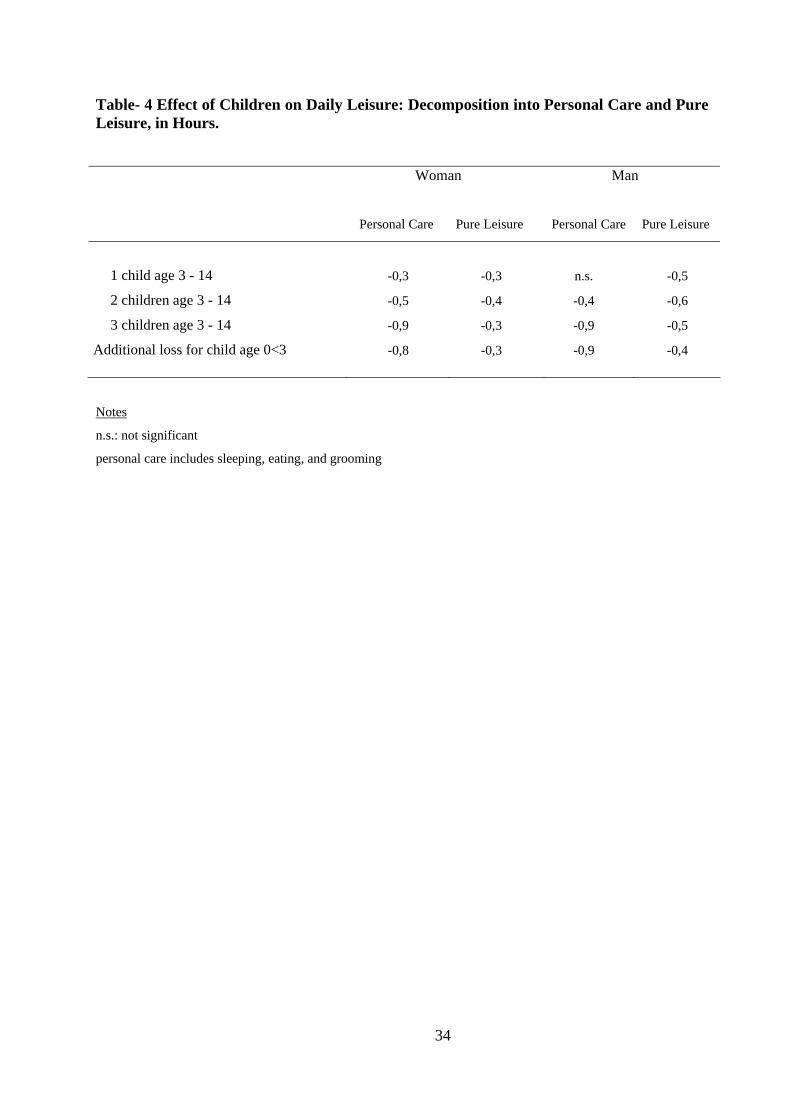
Table- 4 Effect of Children on Daily Leisure: Decomposition into Personal Care and Pure Leisure, in Hours.

Woman Man

Personal Care Pure Leisure Personal Care Pure Leisure

1 child age 3 - 14 -0,3 -0,3 n.s. -0,5

2 children age 3 - 14 -0,5 -0,4 -0,4 -0,6

3 children age 3 - 14 -0,9 -0,3 -0,9 -0,5

Additional loss for child age 0<3 -0,8 -0,3 -0,9 -0,4

Notes

n.s.: not significant

personal care includes sleeping, eating, and grooming

34