Time-Accurate Numerical Prediction of Free Flight Aerodynamics of a Finned Projectile

by Jubaraj Sahu

ARL-TR-3603 September 2005 Approved for public release; distribution is unlimited.

NOTICES

Disclaimers The findings in this report are not to be construed as an official Department of the Army position unless so designated by other authorized documents. Citation of manufacturer’s or trade names does not constitute an official endorsement or approval of the use thereof. DESTRUCTION NOTICE Destroy this report when it is no longer needed. Do not return it to the originator.

Army Research Laboratory Aberdeen Proving Ground, MD 21005-5066

ARL-TR-3603 September 2005

Time-Accurate Numerical Prediction of Free Flight Aerodynamics of a Finned Projectile

Jubaraj Sahu Weapons and Materials Research Directorate, ARL

Approved for public release; distribution is unlimited.

ii

REPORT DOCUMENTATION PAGE Form Approved OMB No. 0704-0188

Public reporting burden for this collection of information is estimated to average 1 hour per response, including the time for reviewing instructions, searching existing data sources, gathering and maintaining the data needed, and completing and reviewing the collection information. Send comments regarding this burden estimate or any other aspect of this collection of information, including suggestions for reducing the burden, to Department of Defense, Washington Headquarters Services, Directorate for Information Operations and Reports (0704-0188), 1215 Jefferson Davis Highway, Suite 1204, Arlington, VA 22202-4302. Respondents should be aware that notwithstanding any other provision of law, no person shall be subject to any penalty for failing to comply with a collection of information if it does not display a currently valid OMB control number. PLEASE DO NOT RETURN YOUR FORM TO THE ABOVE ADDRESS.

1. REPORT DATE (DD-MM-YYYY)

September 2005 2. REPORT TYPE

Final 3. DATES COVERED (From - To)

March 2004 to August 2005 5a. CONTRACT NUMBER

5b. GRANT NUMBER

4. TITLE AND SUBTITLE

Time-Accurate Numerical Prediction of Free Flight Aerodynamics of a Finned Projectile

5c. PROGRAM ELEMENT NUMBER

5d. PROJECT NUMBER

1L1622618.AH80

5e. TASK NUMBER

6. AUTHOR(S)

Jubaraj Sahu (ARL)

5f. WORK UNIT NUMBER

7. PERFORMING ORGANIZATION NAME(S) AND ADDRESS(ES)

U.S. Army Research Laboratory Weapons and Materials Research Directorate Aberdeen Proving Ground, MD 21005-5066

8. PERFORMING ORGANIZATION REPORT NUMBER ARL-TR-3603

10. SPONSOR/MONITOR’S ACRONYM(S) 9. SPONSORING/MONITORING AGENCY NAME(S) AND ADDRESS(ES)

11. SPONSOR/MONITOR’S REPORT NUMBER(S)

12. DISTRIBUTION/AVAILABILITY STATEMENT

Approved for public release; distribution is unlimited.

13. SUPPLEMENTARY NOTES

14. ABSTRACT

This report describes a new multi-disciplinary computational study undertaken to compute the flight trajectories and to simultaneously predict the unsteady free flight aerodynamics of a finned projectile configuration. Actual flight trajectories are computed by an advanced coupled computational fluid dynamics (CFD)-rigid body dynamics technique. An advanced time-accurate Navier-Stokes computational technique has been used in CFD to compute the unsteady aerodynamics associated with the free flight of the finned projectile at supersonic speeds. Computed positions and orientations of the projectile have been compared with actual data measured from free flight tests and are found to be generally in good agreement. Predicted aerodynamics forces and moments also compare well with the forces and moments used in the six-degree-of-freedom fits of the results of the same tests. Unsteady numerical results obtained from the coupled method show the aerodynamic forces and moments and the flight path of the projectile.

15. SUBJECT TERMS

coupled CFD-RBD; finned projectile; flow control; projectile aerodynamics; time accurate; unsteady

16. SECURITY CLASSIFICATION OF: 19a. NAME OF RESPONSIBLE PERSON

Jubaraj Sahu a. REPORT

Unclassified b. ABSTRACT

Unclassified c. THIS PAGE

Unclassified

17. LIMITATIONOF ABSTRACT

SAR

18. NUMBER OF PAGES

25

19b. TELEPHONE NUMBER (Include area code)

410-278-3707 Standard Form 298 (Rev. 8/98)

Prescribed by ANSI Std. Z39.18

iii

Contents

List of Figures iv

Acknowledgments v

1. Introduction 1

2. Solution Technique 3 2.1 Dual Time Stepping.........................................................................................................4 2.2 Grid Movement ...............................................................................................................4 2.3 Six-Degree-of-Freedom Coupling...................................................................................5

3. Results and Discussion 6

4. Summary and Conclusions 13

5. References 15

Distribution List 17

iv

List of Figures

Figure 1. Finned projectile configuration. ......................................................................................6 Figure 2. Computational grid near the projectile. ...........................................................................7 Figure 3. Expanded view of the grid in the base region. ................................................................7 Figure 4. Computed z distance versus range. .................................................................................8 Figure 5. Computed y distance versus range. .................................................................................9 Figure 6. Euler pitch angle distance versus range...........................................................................9 Figure 7. Euler yaw angle versus range. .......................................................................................10 Figure 8. Motion plot (a) computation, and (b) flight test. ...........................................................11 Figure 9. Total angle of attack versus range. ................................................................................12 Figure 10. Angle of attack and side slip versus range. .................................................................12 Figure 11. Comparison of earth-fixed aerodynamic forces and moments....................................14

v

Acknowledgments

This work was accomplished as part of a grand challenge project jointly sponsored by the Department of Defense High Performance Computing Modernization program and the U.S. Army Research Laboratory (ARL). The author wishes to thank Dr. Sukumar Chakravarthy of the Metacomp Technologies for his technical assistance on some of the issues on the coupling techniques between computational fluid dynamics and rigid body dynamics. The author also wishes to thank Mr. Wayne Hathaway of Arrow Tech Associates for providing expert advice and helping with the 6-degree-of-freedom simulations with their software, ARFDAS (Aeroballistics Research Facility Data Analysis System). Thanks are also due Ms. Karen Heavey of ARL for her help in the grid generation. The scientific visualization and the computational support of ARL’s Major Shared Resource Center are greatly appreciated.

vi

INTENTIONALLY LEFT BLANK

1

1. Introduction

The prediction of aerodynamic coefficients for projectile configurations is essential in the assessment of the performance of new designs. Accurate determination of aerodynamics is critical to the low-cost development of new advanced guided projectiles, rockets, missiles, and smart munitions (1,2,3). Advanced weapons, a major part of our armed forces’ arsenal, are vital to the defense of our nation. Precision guided munitions that hit targets more accurately can greatly increase lethality and enhance survivability. To ensure that the United States maintains a strong defense, the Department of Defense (DoD) must continually develop (with fewer dollars) more lethal and effective munitions. The munitions must stay abreast of the latest technology available to our adversaries. The DoD needs ways to develop these advanced weapons without extremely long and costly design cycles. Although actual flight testing of advanced munitions systems will undoubtedly be an essential ingredient in the eventual success of these Army programs, it is expensive and time consuming. Computer simulations can and have provided an effective means of determining the unsteady aerodynamics and flight mechanics of guided projectile systems. The use of high performance computers to model, simulate, and test alternate projectile and missile designs is one response to this requirement. Recent advances made in high performance computing and computational fluid dynamics (CFD) technologies have the potential for greatly reducing the design costs while providing a more detailed understanding of the complex aerodynamics than that achieved through experiments and actual test firings. Understanding the aerodynamics of projectiles, rockets, and missiles is, of course, critical to the design of stable configurations and contributes significantly to the overall performance of weapon systems.

For the past couple of decades, computational capabilities have been developed and employed at the U.S. Army Research Laboratory (ARL) for computing the flight aerodynamics of various projectile and missile configurations (4,5,6,7,8). Three-dimensional (3-D) steady and unsteady Navier-Stokes computational techniques have been used to predict aerodynamics of spinning and fin-stabilized projectiles from subsonic to supersonic speeds. In many applications, 3-D Navier-Stokes computational techniques were employed in conjunction with the Chimera (9,10,11) overlapping grid method to model complex projectile and missile configurations. The Chimera approach was especially useful in CFD modeling of multi-body projectile and missile configurations. An advanced Chimera CFD technique was then extended for accurate numerical calculation of aerodynamics involving multiple bodies with relative motion (2,3). The underlying complex physics and fluid dynamics structure of the aerodynamic interference for multi-body problems were identified. This work showed how maximum savings of time and dollars could be achieved when CFD is brought into weapon system development programs early in the design phase.

2

Improved computer technology and state-of-the-art numerical procedures now enable solutions to complex, 3-D problems associated with projectile and missile aerodynamics. In particular, our recent focus has been directed at the development and application of advanced predictive capabilities to compute unsteady (12,13) projectile aerodynamics. Accurate numerical modeling of the unsteady aerodynamics was found to be challenging and required the use of time-accurate solutions techniques. Recently, the time-accurate technique was used to obtain improved results for Magnus moment and roll damping moment of a spinning projectile at transonic and subsonic speeds (13). Other recent examples have shown the use of time-accurate Navier-Stokes techniques to predict dynamic derivative such as the pitch-damping coefficient (14,15). Recent advances made in CFD now allow one to compute static and dynamic derivatives, which, in turn, make it possible to predict the in-flight motion of projectiles with the numerical data derived solely from CFD. This has been recently demonstrated for a family of axisymmetric projectiles at supersonic speeds (16). The present work is focused on the coupling of CFD and rigid body dynamics (RBD) techniques for simultaneous prediction of the unsteady free-flight aerodynamics and the flight trajectory of projectiles. Our goal is to be able to perform time-accurate multi-disciplinary coupled CFD-RBD computations for the entire flight trajectory of a complex guided projectile system.

Knowledge of the detailed aerodynamics of maneuvering guided smart weapons is rather limited, especially during and after the maneuvers. Multi-disciplinary computations can provide detailed fluid dynamic understanding of the unsteady aerodynamics processes involving the maneuvering flight of modern guided weapon systems. Such knowledge cannot be easily obtained by any other means. The computational technology involving CFD and RBD is now mature and can be used to determine the unsteady aerodynamics associated with the entire mission trajectory of the munitions. These multi-disciplinary computations can lead to better experimental test designs and much better returns for full-scale flight tests. More importantly, they can provide physical insight of fluid mechanics processes that may not be gained from experimental techniques and flight tests.

The advanced CFD capability used here solves the Navier-Stokes equations (17), incorporates unsteady boundary conditions and a special coupling procedure. The present research is a big step forward in that it allows “virtual fly-out” of projectiles on the super-computers and allows numerical prediction of the actual fight paths of a projectile and all the associated unsteady free flight aerodynamics with coupled CFD-RBD techniques in an integrated manner. The following sections describe the solution technique, coupled CFD-RBD procedure, and the computed results obtained for a finned projectile at supersonic speeds.

3

2. Solution Technique

At ARL, research efforts are continuing to perform real-time multi-disciplinary coupled CFD-RBD aerodynamic computations for the entire flight trajectory of a complex guided projectile system. In order to save computer time, our first attempt was to use a quasi-unsteady approach (4). The quasi-unsteady approach relies on Navier-Stokes equations and six-degree-of-freedom (6-DOF) computations to compute a missile trajectory. A degree of freedom is a displacement quantity that defines the location and orientation of an object. In 3-D space, a rigid object has six degrees of freedom: three translations and three rotations. The 6-DOF code computes linear and angular velocities as well as the orientation of the missile, which are used as input to the CFD code. The quasi-unsteady approach uses the following simple procedure to compute a missile trajectory.

1. A CFD solver repeatedly solves the Navier-Stokes equations to obtain missile flow field solutions.

2. A sequence of average values for the forces and moments is generated from the flow field solutions when the consecutive maximum and minimum values are averaged to determine the forces and moments to be used as input in the 6-DOF computations.

3. The 6-DOF computations are performed.

4. With the new initial conditions from the 6-DOF computations, a true increment in time is taken, and the CFD solver computes a new set of solutions. These steps are repeated until the length of the desired trajectory is reached.

A second approach that could be used is the real-time accurate approach. This is the preferred approach and is used in the present work; however, the computations require much greater computer resources. The real-time accurate approach also requires that the 6-DOF body dynamics be computed at each repetition of the flow solver. Both the quasi-unsteady and the real-time accurate approach require a CFD solver.

The CFD capability used here solves the Navier-Stokes equations and incorporates advanced boundary conditions and grid motion capabilities. The present numerical study is a big step forward and a direct extension of that research which now includes numerical simulation of the actual fight paths of the projectile using coupled CFD-RBD techniques with a real-time accurate approach. The complete set of 3-D time-dependent Navier-Stokes equations is solved in a time-accurate manner for simulations of actual flights. A commercially available code, CFD++ (17,18,19,20), is used for the time-accurate unsteady CFD simulations. The basic numerical framework in the code contains unified grid, unified physics, and unified computing features. The user is referred to these references for details of the basic numerical framework.

4

The 3-D, time-dependent Reynolds-averaged Navier Stokes (RANS) equations are solved by the following finite volume method:

[ ] ∫∫∫ =⋅−+VV

dVdAdVt

HGFW∂∂ (1)

in which W is the vector of conservative variables, F and G are the inviscid and viscous flux vectors, respectively, H is the vector of source terms, V is the cell volume, and A is the surface area of the cell face. Second order discretization was used for the flow variables and the turbulent viscosity equation. The turbulence closure is based on topology-parameter-free formulations. Two-equation higher order RANS turbulence models (20) were used for the computation of turbulent flows. These models are ideally suited to unstructured book-keeping and massively parallel processing because of their independence from constraints related to the placement of boundaries and/or zonal interfaces. For computations of unsteady flow fields that are of interest here, dual time stepping (as described next) was used to achieve the desired time accuracy. In addition, the projectile in the coupled CFD-RBD simulation, along with its grid, actually moves and rotates as it flies down range.

2.1 Dual Time Stepping

The “dual time-stepping mode” of the code was used to perform the transient flow simulations. The term “dual time step” implies the use of two time steps. The first is an “outer” or global (and physical) time step that corresponds to the time discretization of the physical time variation term. This time step can be chosen directly by the user and is typically set to a value to represent 1/100 of the period of oscillation expected or forced in the transient flow. It is also applied to every cell and is not spatially varying.

An artificial or “inner” or “local” time variation term is added to the basic physical equations. This time step and corresponding “inner iteration” strategy is chosen to help satisfy the physical transient equations to the desired degree. If the inner iterations converge, then the outer physical transient equations (or their discretization) are satisfied exactly; otherwise, they are satisfied approximately. For the inner iterations, the time step is allowed to vary spatially. Also, relaxation with multi-grid (algebraic) acceleration is employed to reduce the residues of the physical transient equations. It is found that an order of magnitude reduction in the residues is usually sufficient to produce a good transient iteration. This may require a few internal iterations to achieve (between 3 and 10), depending on the magnitude of the outer time step, the nature of the problem, the nature of the boundary conditions, and the consistency of the mesh with respect to the physics available.

2.2 Grid Movement

Grid velocity is assigned to each mesh point. This general capability can be tailored for many specific situations. For example, the grid point velocities can be specified to correspond to a

5

spinning projectile. In this case, the grid speeds are assigned as if the grid were attached to the projectile and spinning with it. Similarly, to account for RBD, the grid point velocities can be set as if the grid were attached to the rigid body with 6-DOF.

A proper treatment of grid motion requires careful attention to the details of the implementation of the algorithm applied to every mesh point and mesh cell so that no spurious numerical effects are created. For example, a required consistency condition is that free stream uniform flow be preserved for arbitrary meshes and arbitrary mesh velocities. CFD++ satisfies this requirement.

Another important aspect concerns how boundary conditions are affected by grid velocities. Consider here the two significant classes of boundary conditions: slip or no slip at a wall and far-field boundary. In CFD++, both are treated in a manner that works seamlessly with or without mesh velocities. In both cases, consider the contra-variant velocity which includes the effect of grid motion. Effectively, it is the normal component of the velocity relative to the mesh. At the body surface, it is set to zero. For a no-slip wall, the tangential component of the velocity is required to be equal to the mesh velocity, by default. Effectively, this assures that the velocity of the mesh is equal to the velocity of the flow at the body. At a far-field boundary, the sign of the contra-variant velocity determines inflow (negative sign) or outflow (positive sign). The magnitude of the contra-variant velocity is compared with the local speed of sound, helping to define one of four possibilities: supersonic inflow, supersonic outflow, subsonic inflow, or subsonic outflow. The characteristics theory is applied to determine what and how much information is applied as the boundary condition for each type and the consistency of the mesh with respect to the physics at hand.

2.3 Six-Degree-of-Freedom Coupling

In CFD++, two modes are available to help simulate RBD: an uncoupled mode and a coupled mode. The coupling refers to the interaction between the aerodynamic forces/moments and the dynamic response of the projectile/body to these forces and moments. In both modes, the forces and moments are computed every time step and reported to the user. In the coupled mode, the forces and moments are passed to a 6-DOF module that computes the body’s response to the forces and moments. The response is converted into translational and rotational accelerations, which are integrated to result in translational and rotational velocities and are integrated once more to result in linear position and angular orientation. The 6-DOF RBD module uses quaternions to define the angular orientations. However, these are easily translated into Euler angles. From the dynamic response, the grid point locations and grid point velocities are set. In the uncoupled mode, the forces and moments are not coupled with the RBD module. The motion of the projectile is kinematic only and depends on the initial linear and angular velocities prescribed.

Typically, we begin with a computation performed in “steady state mode” with the grid velocities prescribed to account only for the translational motion component of the complete set

6

of initial conditions to be prescribed. At this stage, we also impose the angular orientations from the initial conditions. The complete set of initial conditions includes translational and rotational velocity components along with initial position and angular orientation. With a fixed translational velocity, we obtain a steady state solution. This becomes the initial condition for the next step which involves adding only the spin component of the projectile. With the addition of spin, time-accurate calculations are performed for a few cycles of spin until converged periodic forces and moments are obtained. A sufficient number of time steps are performed so that the angular orientation for the spin axis corresponds to the prescribed initial conditions. All this is performed in an uncoupled mode. The angular velocity initial conditions associated with the non-spin rotational modes are then added. The mesh is translated back to the desired initial position, the non-spin rotational velocity initial conditions are turned on, and computations are performed in the coupled mode.

3. Results and Discussion

Time-accurate unsteady numerical computations were performed with Navier-Stokes and coupled 6-DOF methods to predict the unsteady flow fields, aerodynamic forces and moments, and the flight paths of a finned projectile at supersonic speeds. In all cases, full 3-D computations were performed and no symmetry was used.

The supersonic projectile modeled in this study is an ogive-cylinder-finned configuration (see figure 1). The length of the projectile is 121 mm and the diameter is 13 mm. The ogive nose is 98.6 mm long and the afterbody has a 22.3-mm, 2.5-degree boat-tail. Four fins are situated on the back end of the projectile. Each fin is 22.3 mm long and 10.16 mm thick. The computa-tional mesh for the 25-mm projectile model is a C-grid (see figure 2) consisting of seven zones. The first zone encompasses the entire projectile body, from the tip of the nose to the end of the fins. In general, most of the grid points are clustered in the afterbody fin region. Figure 2 shows a 3-D view of the full projectile mesh. The total number of grid points is 4 million for the full computational grid. Figure 3 shows an expanded view of the grid in the base region. The first grid point spacing from the projectile body is chosen to achieve a y+ value of 1.0.

Figure 1. Finned projectile configuration.

7

Figure 2. Computational grid near the projectile.

Figure 3. Expanded view of the grid in the base region.

Here, the primary interest is in the development and application of coupled CFD and RBD techniques for accurate simulation of the free-flight aerodynamics and flight dynamics of the projectile in supersonic flight. The first step here was to obtain the steady state results for this projectile at a given initial supersonic velocity. Also imposed were the angular orientations at this stage. Corresponding converged steady state solution was then used as the starting condition along with the other initial conditions for the computation of coupled CFD-RBD runs. Numerical computations have been made for these cases at initial velocities of 1037 and

8

1034 m/s, depending on whether the simulations were started from the muzzle or a small distance away from it. The corresponding initial angles of attack were α = 0.5 degree or 4.9 degrees, and initial spin rates were 2800 or 2500 radians per second, respectively.

Figures 4 and 5 show the computed z and y distances as a function of x (or, the range). The computed results are shown in solid lines and are compared with the data measured from actual flight tests. For the computed results, the aerodynamic forces and moments were completely obtained through CFD. One simulation started from the gun muzzle and the other from the first station away from the muzzle where the actual data were measured. The first station was about 4.9 m from the muzzle. Both sets of results are generally found to be in good agreement with the measured data, although there is a small discrepancy between the two sets of computed results. Both y and z distances are found to increase with increasing x distance.

0.10

0.15

0.20

0.25

0.30

0.35

0.40

0.0 10.0 20.0 30.0 40.0 50.0 60.0 70.0 80.0

Range, m

Z-C

oord

, m

Experimental DataCFDCFD (Muz)

Figure 4. Computed z distance versus range.

Figure 6 shows the variation of the Euler pitch angle with distance traveled. As seen in this figure, the amplitude and frequency in the Euler pitch angle variation are predicted very well by the computed results and match extremely well with the data from the flight tests. Both sets of computations, whether they started from the muzzle or the first station away from the muzzle, yield essentially the same results. One can also clearly see that the amplitude damps as the projectile flies down range, i.e., with increasing x distance. Figure 7 shows similar behavior with Euler yaw angle with x distance. In this case, however, the yaw angle damps somewhat in the beginning to a 20-m range and then the amplitude stays within +0.5 and -0.5 degree for the rest of the flight. The computed results again compare very well with the measured data from the flight tests.

9

0.10

0.15

0.20

0.25

0.30

0.35

0.40

0.0 10.0 20.0 30.0 40.0 50.0 60.0 70.0 80.0

Range, m

Y-C

oord

, m

Experimental DataCFDCFD (Muz)

Figure 5. Computed y distance versus range.

-8.00

-6.00

-4.00

-2.00

0.00

2.00

4.00

6.00

8.00

0.0 10.0 20.0 30.0 40.0 50.0 60.0 70.0 80.0

Range, m

Thet

a, d

eg

Experimental DataCFD (FS)CFD (Muz)

Figure 6. Euler pitch angle distance versus range.

10

-8.00

-6.00

-4.00

-2.00

0.00

2.00

4.00

6.00

8.00

0.0 10.0 20.0 30.0 40.0 50.0 60.0 70.0 80.0

Range, m

Psi,

deg

Experimental DataCFD (FS)CFD (Muz)

Figure 7. Euler yaw angle versus range.

The time histories of the pitch and yaw angles are often customarily presented as a motion plot where the pitch angle is plotted versus the yaw angle during the flight of the projectile. The motion plot represents the path traversed by the nose of the projectile during the flight trajectory (looking forward from the back of the projectile). Such a plot is shown in figure 8. This figure shows the comparison of the motion plots obtained from the numerical simulations and the 6-DOF analysis of the flight results from ARFDAS (Aeroballistics Research Facility Data Analysis System) (21). Computed results match very well with the experimental flight test results.

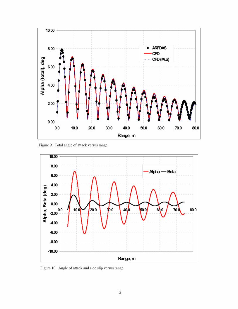
Figures 9 and 10 show the computed total angle of attack and the individual components (angle of attack and side slip), respectively, as a function of the range. These quantities are not directly measured in the actual tests. However, they can be easily derived from the “6-DOF fits” of the actual data. Figure 9 shows the comparison of the total angle of attack derived from such an analysis with the computed results. Computed results include two simulations with different starting conditions, and both sets of these results match quite well with the data derived from the usual 6-DOF fits. All results show the total angle of attack decreasing with increasing range or x distance. Figure 10 shows both component angles: angle of attack and the side slip.

11

(a)

-8 -6 -4 -2 0 2 4 6 8

-12 -10 -8 -6 -4 -2 0 2 4 6 8 10 12 Psi

(b)

Figure 8. Motion plot (a) computation, and (b) flight test.

12

0.00

2.00

4.00

6.00

8.00

10.00

0.0 10.0 20.0 30.0 40.0 50.0 60.0 70.0 80.0

Range, m

Alp

ha (t

otal

), de

gARFDASCFDCFD (Muz)

Figure 9. Total angle of attack versus range.

-10.00

-8.00

-6.00

-4.00

-2.00

0.00

2.00

4.00

6.00

8.00

10.00

0.0 10.0 20.0 30.0 40.0 50.0 60.0 70.0 80.0

Range, m

Alp

ha, B

eta

(deg

)

Alpha Beta

Figure 10. Angle of attack and side slip versus range.

13

Figure 11a and 11b, respectively, shows the comparison of the predicted aerodynamic forces and moments with the ARFDAS results for the same flight conditions. The aerodynamic forces are shown in three directions: x (down range), y (cross range, positive to the left looking from the gun), and z (altitude, positive up). The same sign conventions used in ARFDAS are used in the present study. The moments in this case are taken with respect to the center of gravity of the projectile. As seen in these figures, the predicted unsteady forces and moments have very similar behavior to that used in the 6-DOF analysis of the actual flight test data. The aero-dynamic forces in y and z directions match well with their counterparts in the ARFDAS analysis. However, there is clearly a discrepancy in the comparison of the aerodynamic force in the x direction. Since the drag acts in the negative x direction, the computed drag is over-predicted by 20% to 25%. Although not shown here, a finer grid was used in the steady state mode and the drag results did not change appreciably. Another source of error could come from the inaccurate modeling of the model itself. The actual flight model had a cavity in the base region whereas the computational model has a solid base. A part of the discrepancy can perhaps be attributed to this. Currently, additional work is being performed to find the source of the discrepancy. As seen in figure 11b, the aerodynamic moments are generally found to be in good agreement with the aerodynamic moments used in ARFDAS.

4. Summary and Conclusions

This report describes a new coupled CFD-RBD computational study undertaken to simultaneously determine the flight trajectory and the associated unsteady free-flight aerodynamics of a finned projectile. A 3-D unsteady Navier-Stokes solver is employed to compute the time-accurate aerodynamics associated with the free flight of the finned projectile at supersonic velocities. Computed positions and orientations of the projectile have been compared with actual data measured from free-flight tests and are found to be generally in good agreement. Predicted aerodynamics forces and moments also compare generally well with the forces and moments used in the 6-DOF fits of the results of the same tests except for the force in the x direction. This work demonstrates a coupled method to accurately predict the time-accurate unsteady aerodynamics and the flight trajectories of projectiles at various speeds. Additional work is needed to continue the validation of the computed results with the data and results from other techniques and extraction of the aerodynamic coefficients from the simulations at hand. The present CFD-RBD simulations clearly show the potential capability of the coupled approach and form the basis for future multi-disciplinary, time-dependent computations of advanced maneuvering munitions.

14

-80.00

-60.00

-40.00

-20.00

0.00

20.00

40.00

60.00

0.0 10.0 20.0 30.0 40.0 50.0 60.0 70.0 80.0

Range, m

Forc

es

FxFyFzFx (ARFDAS)Fy (ARFDAS)Fz (ARFDAS)

(a) aerodynamic forces

-3.00

-2.00

-1.00

0.00

1.00

2.00

3.00

0.0 10.0 20.0 30.0 40.0 50.0 60.0 70.0 80.0

Range, m

Mom

ents

MxMyMzMx (ARFDAS)My (ARFDAS)Mz (ARFDAS)

(b) aerodynamic moments

Figure 11. Comparison of earth-fixed aerodynamic forces and moments.

15

5. References

1. Sahu, J.; Heavey, K. R.; Ferry, E. N. Computational Fluid Dynamics for Multiple Projectile Configurations. Proceedings of the Third Overset Composite Grid and Solution Technology Symposium, Los Alamos, NM, October 1996.

2. Sahu, J.; Heavey, K. R.; Nietubicz, C. J. Time-Dependent Navier-Stokes Computations for Submunitions in Relative Motion. Sixth International Symposium on Computational Fluid Dynamics, Lake Tahoe, NV, September 1995.

3. Meakin, R. L. Computations of the Unsteady Flow About a Generic Wing/Pylon/Finned Store Configuration; American Institute of Aeronautics and Astronautics (AIAA) 92-4568-CP, Hilton Head, SC, August 1992.

4. Sahu, J.; Edge, H. L.; DeSpirito, J.; Heavey, K. R.; Ramakrishnan, S. V.; Dinavahi, S.P.G. Applications of Computational Fluid Dynamics to Advanced Guided Munitions. 39th AIAA Aerospace Sciences Meeting, Reno, NV, 8-12 January 2001.

5. Sahu, J.; Edge, H. L.; Dinavahi, S.; Soni, B. Progress on Unsteady Aerodynamics of Maneuvering Munitions. Users Group Meeting Proceedings, Albuquerque, NM, June 2000.

6. Silton, S. I. Navier-Stokes Computations for a Spinning Projectile for Subsonic to Supersonic Speeds. Journal of Spacecraft and Rockets 2005, 42 (2), 223-231.

7. Heavey, K. R.; Sahu, J. Application of Computational Fluid Dynamics to a Monoplane Fixed Wing Missile with Elliptic Cross Sections; ARL-TR-3549; U.S. Army Research Laboratory: Aberdeen Proving Ground, MD, July 2005.

8. Sahu, J.; Silton, S. I.; Heavey, K. R. Navier-Stokes Computations of Supersonic Flow over Complex Missile Configurations. AIAA Paper No. 2004-5456, AIAA 22nd Applied Aerodynamics Conference, Providence, RI, August 16-19, 2004.

9. Steger, J. L.; Dougherty, F. C.; Benek, J. A. A Chimera Grid Scheme. Advances in Grid Generation, edited by K. N. Ghia and U. Ghia, ASME FED-5, June 1983.

10. Meakin, R.; Gomez, R. On Adaptive Refinement and Overset Structured Grids. AIAA Paper No. 97-1858-CP, 1997.

11. Meakin, R. Unsteady Simulation of the Viscous Flow About a V-22 Rotor and Wing in Hover. AIAA-95-3463, August, 1995.

12. Sahu, J. Unsteady CFD Modeling of Aerodynamic Flow Control over a Spinning Body with Synthetic Jet. AIAA Paper 2004-0747, Reno, NV, 5-8 January 2004.

16

13. DeSpirito, J.; Heavey, K. R. CFD Computation of Magnus Moment and Roll Damping Moment of a Spinning Projectile. AIAA Paper No. 2004-4713, Atmospheric Flight Mechanics Conference, Providence, RI, August 2004.

14. Oktay, E.; Akay, H. U. CFD Predictions of Dynamic Derivatives for Missiles. AIAA Paper No. 2002-0276, January 2002.

15. Park, S. H.; Kwon, J. H. Navier-Stokes Computations of Stability Derivatives for Symmetric Projectiles. AIAA Paper No. 2004-0014, January 2004.

16. Weinacht, P. Prediction of Projectile Performance, Stability, and Free-Flight Motion Using Computational Fluid Dynamics; ARL-TR-3015; U.S. Army Research Laboratory: Aberdeen Proving Ground, MD, July 2003.

17. Peroomian, O.; Chakravarthy, S.; Goldberg, U. A ‘Grid-Transparent’ Methodology for CFD. AIAA Paper 97-07245, 1997.

18. Batten, P.; Goldberg U.; Chakravarthy, S. Sub-grid Turbulence Modeling for Unsteady Flow with Acoustic Resonance. AIAA Paper 00-0473, 38th AIAA Aerospace Sciences Meeting, Reno, NV, January 2000.

19. Peroomian, O.; Chakravarthy, S.; Palaniswamy, S.; Goldberg, U. Convergence Acceleration for Unified-Grid Formulation Using Preconditioned Implicit Relaxation. AIAA Paper 98-0116, 1998.

20. Goldberg, U. C.; Peroomian, O.; Chakravarthy, S. A Wall-Distance-Free K-E Model With Enhanced Near-Wall Treatment. ASME Journal of Fluids Engineering 1998, 120, pp. 457-462.

21. Arrow Tech Associates. ARFDAS Technical Manual. South Burlington, VT, 2001.

22. Costello, M. Extended Range of a Gun Launched Smart Projectile Using Controllable Canards. Shock and Vibration 2001, 8 (3-4), 203-213.

17

NO. OF COPIES ORGANIZATION 1 DEFENSE TECHNICAL (PDF INFORMATION CTR ONLY) DTIC OCA 8725 JOHN J KINGMAN RD STE 0944 FORT BELVOIR VA 22060-6218 1 US ARMY RSRCH DEV & ENGRG CMD SYSTEMS OF SYSTEMS INTEGRATION AMSRD SS T 6000 6TH ST STE 100 FORT BELVOIR VA 22060-5608 1 INST FOR ADVNCD TCHNLGY THE UNIV OF TEXAS AT AUSTIN 4030-2 W BRAKER LN AUSTIN TX 78759-5316 1 DIRECTOR US ARMY RESEARCH LAB IMNE ALC IMS 2800 POWDER MILL RD ADELPHI MD 20783-1197 1 DIRECTOR US ARMY RESEARCH LAB AMSRD ARL CI OK TL 2800 POWDER MILL RD ADELPHI MD 20783-1197 2 DIRECTOR US ARMY RESEARCH LAB AMSRD ARL CS IS T 2800 POWDER MILL RD ADELPHI MD 20783-1197 1 COMMANDER NAVAL SURFACE WARFARE CNTR ATTN CODE B40 DR W YANTA DAHLGREN VA 22448-5100 1 COMMANDER NAVAL SURFACE WARFARE CNTR ATTN CODE 420 DR A WARDLAW INDIAN HEAD MD 20640-5035 1 AIR FORCE ARMAMENT LAB ATTN AFATL/FXA DAVE BELK EGLIN AFB FL 32542-5434

NO. OF COPIES ORGANIZATION 3 COMMANDER US ARMY TACOM-ARDEC ATTN AMSTA AR FSF T J GRAU H HUDGINS W KOENIG BLDG 382 PICATINNY ARSENAL NJ 07806-5000 1 COMMANDER US ARMY TACOM ATTN AMSTA AR CCH B P VALENTI BLDG 65-S PICATINNY ARSENAL NJ 07806-5001 1 COMMANDER US ARMY ARDEC ATTN SFAE FAS SD M DEVINE PICATINNY ARSENAL NJ 07806-5001 1 NAVAL AIR WARFARE CENTER ATTN DAVID FINDLAY MS 3 BLDG 2187 PATUXENT RIVER MD 20670 1 UNIV OF TEXAS AT ARLINGTON DEPT OF MECH AND AEROSPACE ENG ATTN DR J C DUTTON BOX 19018 500 W FIRST ST ARLINGTON TX 76019-0018 1 COMMANDER US ARMY TACOM-ARDEC ATTN AMCPM DS MO P BURKE BLDG 162S PICATINNY ARSENAL NJ 07806-5000 ABERDEEN PROVING GROUND 1 DIRECTOR US ARMY RSCH LABORATORY ATTN AMSRD ARL CI OK TECH LIB BLDG 4600 15 DIR USARL AMSRD ARL WM J SMITH D LYON AMSRD ARL WM B T ROSENBERGER AMSRD ARL WM BC P PLOSTINS J DESPIRITO B GUIDOS K HEAVEY J NEWILL J SAHU (2 CYS) S SILTON P WEINACHT AMSRD ARL WM BD B FORCH AMSRD ARL WM BF S WILKERSON AMSRD ARL CI HC R NOAK

18

NO. OF COPIES ORGANIZATION 1 JOHN A EDWARDS DSTL FELLOW MCM DEPARTMENT DSTL FORT HALSTEAD SEVENOAKS KENT NT14 7BP UK