Beyond Worst-Case Analysis

Tim Roughgarden∗

June 27, 2018

1 Introduction

Comparing different algorithms is hard. For almost any pair of algorithms and measure of algorithmperformance—like running time or solution quality—each algorithm will perform better than theother on some inputs.1 For example, the insertion sort algorithm is faster than merge sort onalready-sorted arrays but slower on many other inputs. When two algorithms have incomparableperformance, how can we deem one of them “better than” the other?

Worst-case analysis is a specific modeling choice in the analysis of algorithms, where the overallperformance of an algorithm is summarized by its worst performance on any input of a given size.The “better” algorithm is then the one with superior worst-case performance. Merge sort, with itsworst-case asymptotic running time of Θ(n log n) for arrays of length n, is better in this sense thaninsertion sort, which has a worst-case running time of Θ(n2).

While crude, worst-case analysis can be tremendously useful, and it is the dominant paradigmfor algorithm analysis in theoretical computer science. A good worst-case guarantee is the best-case scenario for an algorithm, certifying its general-purpose utility and absolving its users fromunderstanding which inputs are relevant to their applications. Remarkably, for many fundamentalcomputational problems, there are algorithms with excellent worst-case performance guarantees.The lion’s share of an undergraduate algorithms course comprises algorithms that run in linear ornear-linear time in the worst case.

For many problems a bit beyond the scope of an undergraduate course, however, the downsideof worst-case analysis rears its ugly head. We next review three classical examples where worst-case analysis gives misleading or useless advice about how to solve a problem; further examples inmodern machine learning are described later. These examples motivate the alternatives to worst-case analysis described in the rest of the article.2

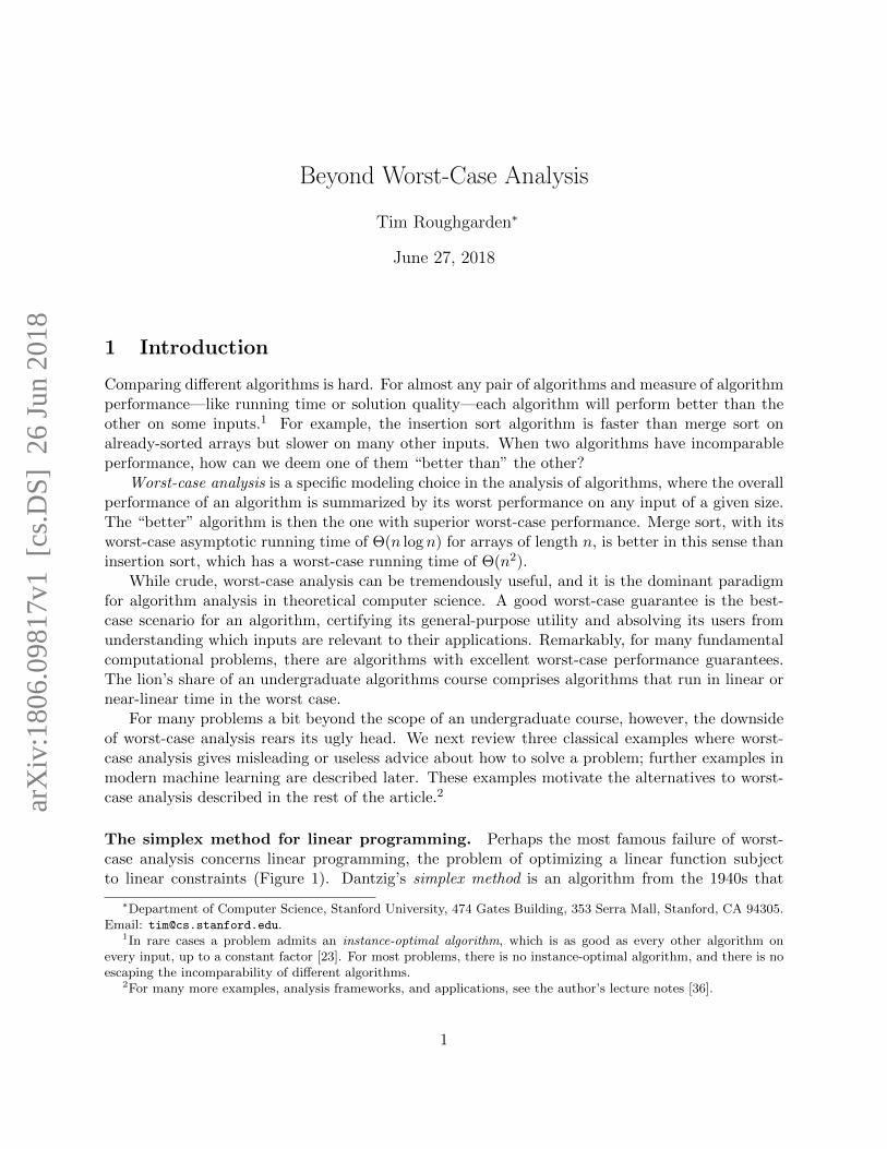
The simplex method for linear programming. Perhaps the most famous failure of worst-case analysis concerns linear programming, the problem of optimizing a linear function subjectto linear constraints (Figure 1). Dantzig’s simplex method is an algorithm from the 1940s that

∗Department of Computer Science, Stanford University, 474 Gates Building, 353 Serra Mall, Stanford, CA 94305.Email: tim@cs.stanford.edu.

1In rare cases a problem admits an instance-optimal algorithm, which is as good as every other algorithm onevery input, up to a constant factor [23]. For most problems, there is no instance-optimal algorithm, and there is noescaping the incomparability of different algorithms.

2For many more examples, analysis frameworks, and applications, see the author’s lecture notes [36].

1

arX

iv:1

806.

0981

7v1

[cs

.DS]

26

Jun

2018

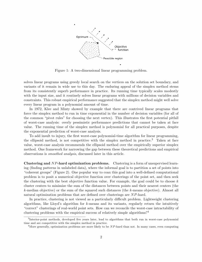
Figure 1: A two-dimensional linear programming problem.

solves linear programs using greedy local search on the vertices on the solution set boundary, andvariants of it remain in wide use to this day. The enduring appeal of the simplex method stemsfrom its consistently superb performance in practice. Its running time typically scales modestlywith the input size, and it routinely solves linear programs with millions of decision variables andconstraints. This robust empirical performance suggested that the simplex method might well solveevery linear program in a polynomial amount of time.

In 1972, Klee and Minty showed by example that there are contrived linear programs thatforce the simplex method to run in time exponential in the number of decision variables (for all ofthe common “pivot rules” for choosing the next vertex). This illustrates the first potential pitfallof worst-case analysis: overly pessimistic performance predictions that cannot be taken at facevalue. The running time of the simplex method is polynomial for all practical purposes, despitethe exponential prediction of worst-case analysis.

To add insult to injury, the first worst-case polynomial-time algorithm for linear programming,the ellipsoid method, is not competitive with the simplex method in practice.3 Taken at facevalue, worst-case analysis recommends the ellipsoid method over the empirically superior simplexmethod. One framework for narrowing the gap between these theoretical predictions and empiricalobservations is smoothed analysis, discussed later in this article.

Clustering and NP -hard optimization problems. Clustering is a form of unsupervised learn-ing (finding patterns in unlabeled data), where the informal goal is to partition a set of points into“coherent groups” (Figure 2). One popular way to coax this goal into a well-defined computationalproblem is to posit a numerical objective function over clusterings of the point set, and then seekthe clustering with the best objective function value. For example, the goal could be to choose kcluster centers to minimize the sum of the distances between points and their nearest centers (thek-median objective) or the sum of the squared such distances (the k-means objective). Almost allnatural optimization problems that are defined over clusterings are NP -hard.

In practice, clustering is not viewed as a particularly difficult problem. Lightweight clusteringalgorithms, like Lloyd’s algorithm for k-means and its variants, regularly return the intuitively“correct” clusterings of real-world point sets. How can we reconcile the worst-case intractability ofclustering problems with the empirical success of relatively simple algorithms?4

3Interior-point methods, developed five years later, lead to algorithms that both run in worst-case polynomialtime and are competitive with the simplex method in practice.

4More generally, optimization problems are more likely to be NP -hard than not. In many cases, even computing

2

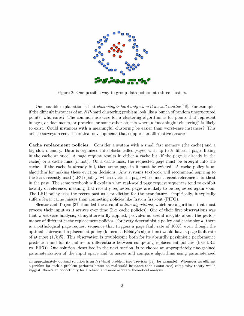
Figure 2: One possible way to group data points into three clusters.

One possible explanation is that clustering is hard only when it doesn’t matter [18]. For example,if the difficult instances of an NP -hard clustering problem look like a bunch of random unstructuredpoints, who cares? The common use case for a clustering algorithm is for points that representimages, or documents, or proteins, or some other objects where a “meaningful clustering” is likelyto exist. Could instances with a meaningful clustering be easier than worst-case instances? Thisarticle surveys recent theoretical developments that support an affirmative answer.

Cache replacement policies. Consider a system with a small fast memory (the cache) and abig slow memory. Data is organized into blocks called pages, with up to k different pages fittingin the cache at once. A page request results in either a cache hit (if the page is already in thecache) or a cache miss (if not). On a cache miss, the requested page must be brought into thecache. If the cache is already full, then some page in it must be evicted. A cache policy is analgorithm for making these eviction decisions. Any systems textbook will recommend aspiring tothe least recently used (LRU) policy, which evicts the page whose most recent reference is furthestin the past. The same textbook will explain why: real-world page request sequences tend to exhibitlocality of reference, meaning that recently requested pages are likely to be requested again soon.The LRU policy uses the recent past as a prediction for the near future. Empirically, it typicallysuffers fewer cache misses than competing policies like first-in first-out (FIFO).

Sleator and Tarjan [37] founded the area of online algorithms, which are algorithms that mustprocess their input as it arrives over time (like cache policies). One of their first observations wasthat worst-case analysis, straightforwardly applied, provides no useful insights about the perfor-mance of different cache replacement policies. For every deterministic policy and cache size k, thereis a pathological page request sequence that triggers a page fault rate of 100%, even though theoptimal clairvoyant replacement policy (known as Belady’s algorithm) would have a page fault rateof at most (1/k)%. This observation is troublesome both for its absurdly pessimistic performanceprediction and for its failure to differentiate between competing replacement policies (like LRUvs. FIFO). One solution, described in the next section, is to choose an appropriately fine-grainedparameterization of the input space and to assess and compare algorithms using parameterized

an approximately optimal solution is an NP -hard problem (see Trevisan [39], for example). Whenever an efficientalgorithm for such a problem performs better on real-world instances than (worst-case) complexity theory wouldsuggest, there’s an opportunity for a refined and more accurate theoretical analysis.

3

guarantees.

2 Models of Typical Instances

Maybe we shouldn’t be surprised that worst-case analysis fails to advocate LRU over FIFO. Theempirical superiority of LRU is due to the special structure in real-world page request sequences—locality of reference—and traditional worst-case analysis provides no vocabulary to speak aboutthis structure.5 This is what work on “beyond worst-case analysis” is all about:

articulating properties of “real-world” inputs, and proving rigorous and meaningful algorithmicguarantees for inputs with these properties.

Research in the area has both a scientific dimension, where the goal is to develop transparentmathematical models that explain empirically observed phenomena about algorithm performance,and an engineering dimension, where the goals are to provide accurate guidance about whichalgorithm to use for a problem and to design new algorithms that perform particularly well on therelevant inputs.

One exemplary result in beyond worst-case analysis is due to Albers et al. [2], for the online pag-ing problem described in the introduction. The key idea is to parameterize page request sequencesaccording to how much locality of reference they exhibit, and then prove parameterized worst-case guarantees. Refining worst-case analysis in this way leads to dramatically more informativeresults.6

Locality of reference is quantified via the size of the working set of a page request sequence.Formally, for a function f : N → N, we say that a request sequence conforms to f if, in everywindow of w consecutive page requests, at most f(w) distinct pages are requested. For example,the identity function f(w) = w imposes no restrictions on the page request sequence. A sequencecan only conform to a sublinear function like f(w) = d

√we or f(w) = d1 + log2we if it exhibits

locality of reference.7

The following worst-case guarantee is parameterized by a number αf (k), between 0 and 1, thatwe discuss shortly; recall that k denotes the cache size. It assumes that the function f is “concave”in the sense that the number of inputs with value x under f (that is, |f−1(x)|) is nondecreasingin x.

Theorem 1 (Albers et al. [2])

(a) For every f and k and every deterministic cache replacement policy, the worst-case page faultrate (over sequences that conform to f) is at least αf (k).

(b) For every f and k and every sequence that conforms to f , the page fault rate of the LRUpolicy is at most αf (k).

5If worst-case analysis has an implicit model of data, then it’s the “Murphy’s Law” data model, where the instanceto be solved is an adversarially selected function of the chosen algorithm. Outside of cryptographic applications, thisis a rather paranoid and incoherent way to think about a computational problem.

6Parameterized guarantees are common in the analysis of algorithms. For example, the field of parameterizedalgorithms and complexity has developed a rich theory around parameterized running time bounds (see the bookby Cygan et al. [16]). Theorem 1 employs an unusually fine-grained and problem-specific parameterization, and inexchange obtains unusually accurate and meaningful results.

7The notation dxe means the number x, rounded up to the nearest integer.

4

(c) There exists a choice of f and k, and a page request sequence that conforms to f , such thatthe page fault rate of the FIFO policy is strictly larger than αf (k).

Parts (a) and (b) prove the worst-case optimality of the LRU policy in a strong sense, f -by-f andk-by-k. Part (c) differentiates LRU from FIFO, as the latter is suboptimal for some (in fact, many)choices of f and k.

The guarantees in Theorem 1 are so good that they are meaningful even when taken at facevalue—for sublinear f ’s, αf (k) goes to 0 reasonably quickly with k. For example, if f(w) = d

√we,

then αf (k) scales with 1/√k. Thus with a cache size of 10,000, the page fault rate is always at

most 1%. If f(w) = d1 + log2we, then αf (k) goes to 0 even faster with k, roughly as k/2k.8

3 Stable Instances

Are point sets with meaningful clusterings easier to cluster than worst-case point sets? We nextdescribe one way to define a “meaningful clustering,” due to Bilu and Linial [12]; for others, seeAckerman and Ben-David [1], Balcan et al. [9], Daniely et al. [18], Kumar and Kannan [29], andOstrovsky et al. [34].

The maximum cut problem. Suppose you have a bunch of data points representing images ofcats and images of dogs, and you’d like to automatically discover these two groups. One approachis to reduce this task to the maximum cut problem, where the goal is to partition the vertices Vof a graph G with edges E and nonnegative edge weights into two groups, while maximizing thetotal weight of the edges that have one endpoint in each group. The reduction forms a completegraph G, with vertices corresponding to the data points, and assigns a weight we to each edge eindicating how dissimilar its endpoints are. The maximum cut of G is a 2-clustering that tends toput dissimilar pairs of points in different clusters.

There are many ways to quantify “dissimilarity” between images, and different definitions mightgive different optimal 2-clusterings of the data points. One would hope that, for a range of reason-able measures of dissimilarity, the maximum cut in the example above would have all cats on oneside and all dogs on the other. In other words, the maximum cut should be invariant under minorchanges to the specification of the edge weights (Figure 3).

Definition 2 (Bilu and Linial [12]) An instance G = (V,E,w) of the maximum cut problemis γ-perturbation stable if, for all ways of multiplying the weight we of each edge e by a factorαe ∈ [1, γ], the optimal solution remains the same.

A perturbation-stable instance has a “clearly optimal” solution—a uniqueness assumption onsteroids—thus formalizing the idea of a “meaningful clustering.” In machine learning parlance,perturbation stability can be viewed as a type of “large margin” assumption.

The maximum cut problem is NP -hard in general. But what about the special case of γ-perturbation-stable instances? As γ increases, fewer and fewer instances qualify as γ-perturbationstable. Is there a sharp stability threshold—a value of γ where the maximum cut problem switchesfrom NP -hard to polynomial-time solvable?

Makarychev et al. [30] largely resolved this question. On the positive side, they showed that if γis at least a slowly growing function of the number of vertices n, then the maximum cut problem

8See Albers et al. [2] for the precise closed-form formula for αf (k) in general.

5

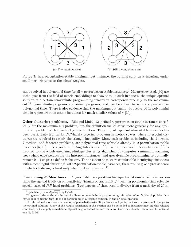
(a) The maximum cut (b) Still the maximum cut

Figure 3: In a perturbation-stable maximum cut instance, the optimal solution is invariant undersmall perturbations to the edges’ weights.

can be solved in polynomial time for all γ-perturbation stable instances.9 Makarychev et al. [30] usetechniques from the field of metric embeddings to show that, in such instances, the unique optimalsolution of a certain semidefinite programming relaxation corresponds precisely to the maximumcut.10 Semidefinite programs are convex programs, and can be solved to arbitrary precision inpolynomial time. There is also evidence that the maximum cut cannot be recovered in polynomialtime in γ-perturbation-stable instances for much smaller values of γ [30].

Other clustering problems. Bilu and Linial [12] defined γ-perturbation-stable instances specif-ically for the maximum cut problem, but the definition makes sense more generally for any opti-mization problem with a linear objective function. The study of γ-perturbation-stable instances hasbeen particularly fruitful for NP -hard clustering problems in metric spaces, where interpoint dis-tances are required to satisfy the triangle inequality. Many such problems, including the k-means,k-median, and k-center problems, are polynomial-time solvable already in 2-perturbation-stableinstances [5, 10]. The algorithm in Angelidakis et al. [5], like its precursor in Awasthi et al. [8], isinspired by the widely-used single-linkage clustering algorithm. It computes a minimum spanningtree (where edge weights are the interpoint distances) and uses dynamic programming to optimallyremove k−1 edges to define k clusters. To the extent that we’re comfortable identifying “instanceswith a meaningful clustering” with 2-perturbation-stable instances, these results give a precise sensein which clustering is hard only when it doesn’t matter.11

Overcoming NP -hardness. Polynomial-time algorithms for γ-perturbation-stable instances con-tinue the age-old tradition of identifying “islands of tractability,” meaning polynomial-time solvablespecial cases of NP -hard problems. Two aspects of these results diverge from a majority of 20th-

9Specifically, γ = Ω(√

logn log logn).10In general, the optimal solution of a linear or semidefinite programming relaxation of an NP -hard problem is a

“fractional solution” that does not correspond to a feasible solution to the original problem.11A relaxed and more realistic version of perturbation-stability allows small perturbations to make small changes to

the optimal solution. Many of the results mentioned in this section can be extended to instances meeting this relaxedcondition, with a polynomial-time algorithm guaranteed to recover a solution that closely resembles the optimalone [5, 9, 30].

6

century research on tractable special cases. First, perturbation-stability is not an easy condition tocheck, in contrast to a restriction like graph planarity or Horn-satisfiability. Instead, the assump-tion is justified with a plausible narrative about why “real-world instances” might satisfy it, atleast approximately. Second, in most work going beyond worst-case analysis, the goal is to studygeneral-purpose algorithms, which are well defined on all inputs, and use the assumed instancestructure only in the algorithm analysis (and not explicitly in its design). The hope is that thealgorithm continues to perform well on many instances not covered by its formal guarantee. Theresults above for mathematical programming relaxations and single-linkage-based algorithms aregood examples of this paradigm.

Analogy with sparse recovery. There are compelling parallels between the recent research onclustering in stable instances and slightly older results in a field of applied mathematics knownas sparse recovery, where the goal is to reverse engineer a “sparse” object from a small numberof clues about it. A common theme in both areas is identifying relatively weak conditions underwhich a tractable mathematical programming relaxation of an NP -hard problem is guaranteed tobe exact, meaning that the original problem and its relaxation have the same optimal solution.

For example, a canonical problem in sparse recovery is compressive sensing, where the goalis to recover an unknown sparse signal (a vector of length n) from a small number m of linearmeasurements of it. Equivalently, given an m × n measurement matrix A with m n and themeasurement results b = Az, the problem is to figure out the signal z. This problem has severalimportant applications, for example in medical imaging. If z can be arbitrary, then the problem ishopeless: since m < n, the linear system Ax = b is underdetermined and has an infinite number ofsolutions (of which z is only one). But many real-world signals are (approximately) k-sparse in asuitable basis for small k, meaning that (almost) all of the mass is concentrated on k coordinates.12

The main results in compressive sensing show that, under appropriate assumptions on A, theproblem can be solved efficiently even when m is only modestly bigger than k (and much smallerthan n) [15, 20]. One way to prove these results is to formulate a linear programming relaxationof the (NP -hard) problem of computing the sparsest solution to Ax = b, and then show that thisrelaxation is exact.

4 Planted and Semi-Random Models

Our next genre of models is also inspired by the idea that interesting instances of a problem shouldhave “clearly optimal” solutions, but differs from the above stability conditions in assuming agenerative model—a specific distribution over inputs. The goal is to design an algorithm that, withhigh probability over the assumed input distribution, computes an optimal solution in polynomialtime.

The planted clique problem. In the maximum clique problem, the input is an undirected graphG = (V,E), and the goal is to identify the largest subset of vertices that are mutually adjacent.This problem is NP -hard, even to approximate by any reasonable factor. Is it easy when there isa particularly prominent clique to be found?

Jerrum [27] suggested the following generative model. There is a fixed set V of n vertices. First,each possible edge (u, v) is included independently with 50% probability. This is also known as an

12For example, audio signals are typically approximately sparse in the Fourier basis, images in the wavelet basis.

7

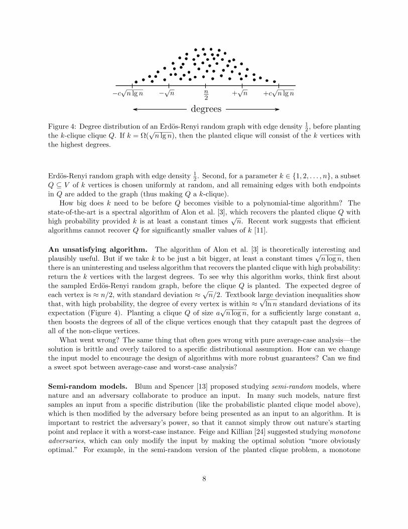
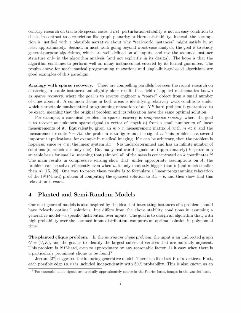
Figure 4: Degree distribution of an Erdos-Renyi random graph with edge density 12 , before planting

the k-clique clique Q. If k = Ω(√n lg n), then the planted clique will consist of the k vertices with

the highest degrees.

Erdos-Renyi random graph with edge density 12 . Second, for a parameter k ∈ 1, 2, . . . , n, a subset

Q ⊆ V of k vertices is chosen uniformly at random, and all remaining edges with both endpointsin Q are added to the graph (thus making Q a k-clique).

How big does k need to be before Q becomes visible to a polynomial-time algorithm? Thestate-of-the-art is a spectral algorithm of Alon et al. [3], which recovers the planted clique Q withhigh probability provided k is at least a constant times

√n. Recent work suggests that efficient

algorithms cannot recover Q for significantly smaller values of k [11].

An unsatisfying algorithm. The algorithm of Alon et al. [3] is theoretically interesting andplausibly useful. But if we take k to be just a bit bigger, at least a constant times

√n log n, then

there is an uninteresting and useless algorithm that recovers the planted clique with high probability:return the k vertices with the largest degrees. To see why this algorithm works, think first aboutthe sampled Erdos-Renyi random graph, before the clique Q is planted. The expected degree ofeach vertex is ≈ n/2, with standard deviation ≈

√n/2. Textbook large deviation inequalities show

that, with high probability, the degree of every vertex is within ≈√

lnn standard deviations of itsexpectation (Figure 4). Planting a clique Q of size a

√n log n, for a sufficiently large constant a,

then boosts the degrees of all of the clique vertices enough that they catapult past the degrees ofall of the non-clique vertices.

What went wrong? The same thing that often goes wrong with pure average-case analysis—thesolution is brittle and overly tailored to a specific distributional assumption. How can we changethe input model to encourage the design of algorithms with more robust guarantees? Can we finda sweet spot between average-case and worst-case analysis?

Semi-random models. Blum and Spencer [13] proposed studying semi-random models, wherenature and an adversary collaborate to produce an input. In many such models, nature firstsamples an input from a specific distribution (like the probabilistic planted clique model above),which is then modified by the adversary before being presented as an input to an algorithm. It isimportant to restrict the adversary’s power, so that it cannot simply throw out nature’s startingpoint and replace it with a worst-case instance. Feige and Killian [24] suggested studying monotoneadversaries, which can only modify the input by making the optimal solution “more obviouslyoptimal.” For example, in the semi-random version of the planted clique problem, a monotone

8

adversary is only allowed to remove edges that are not in the planted clique Q—it cannot removeedges from Q or add edges outside Q.

Semi-random models with a monotone adversary may initially seem no harder than the plantedmodels that they generalize. But let’s return to the planted clique model with k = Ω(

√n log n),

where the “top-k degrees” algorithm succeeds with high probability when there is no adversary.A monotone adversary can easily foil this algorithm in the semi-random planted clique model,by removing edges between clique and non-clique vertices to decrease the degrees of the formerback down to ≈ n/2. Thus the semi-random model forces us to develop smarter, more robustalgorithms.13

For the semi-random planted clique model, Feige and Krauthgamer [24] gave a polynomial-time algorithm that recovers the clique with high probability provided k = Ω(

√n). The spectral

algorithm by Alon et al. [3] achieved this guarantee only in the standard planted clique model, andit does not provide any strong guarantees for the semi-random model. The algorithm of Feige andKrauthgamer [24] instead uses a semidefinite programming relaxation of the problem. Their analysisshows that this relaxation is exact with high probability in the standard planted clique model(provided k = Ω(

√n)), and uses the monotonicity properties of optimal mathematical programming

solutions to argue that this exactness cannot be sabotaged by any monotone adversary.

5 Smoothed Analysis

Smoothed analysis is another example of a semi-random model, now with the order of operationsreversed: an adversary goes first and chooses an arbitrary input, which is then perturbed slightly bynature. Smoothed analysis can be applied to any problem where “small perturbations” make sense,including most problems with real-valued inputs. It can be applied to any measure of algorithmperformance, but has proven most effective for running time analyses.

Like other semi-random models, smoothed analysis has the benefit of potentially escaping worst-case inputs (especially if they are “isolated”), while avoiding overfitting a solution to a specificdistributional assumption. There is also a plausible narrative about why “real-world” inputs arecaptured by this framework: whatever problem you’d like to solve, there are inevitable inaccuraciesin its formulation (from measurement error, uncertainty, and so on).

The simplex method. Spielman and Teng [38] developed the smoothed analysis framework withthe specific goal of proving that bad inputs for the simplex method are exceedingly rare. Average-case analyses of the simplex method from the 1980s (e.g., Borgwardt [14]) provide evidence for thisthesis, but smoothed analysis provides more robust support for it.

The perturbation model in Spielman and Teng [38] is: independently for each entry of theconstraint matrix and right-hand side of the linear program, add a Gaussian (i.e., normal) randomvariable with mean 0 and standard deviation σ.14 The parameter σ interpolates between worst-

13The extensively studied “stochastic block model”generalizes the planted clique model (see e.g. Moore [32]), andis another fruitful playground for semi-random models. Here, the vertices of a graph are partitioned into groups, andthe probability that an edge is present is a function of the groups that contain its endpoints. The responsibility ofan algorithm in this model is to recover the (unknown) vertex partition. This goal becomes provably strictly harderin the presence of a monotone adversary [31].

14This perturbation results in a dense constraint matrix even if the original one was sparse, and for this reasonTheorem 3 is not fully satisfactory. Extending this result to sparsity-preserving perturbations is an important openquestion.

9

case analysis (when σ = 0) and pure average-case analysis (as σ → ∞, the perturbation drownsout the original linear program). The main result states that the expected running time of thesimplex method is polynomial as long as typical perturbations have magnitude at least an inversepolynomial function of the input size (which is small!).

Theorem 3 (Spielman and Teng [38]) For every initial linear program, in expectation over theperturbation to the program, the running time of the simplex method is polynomial in the input sizeand in 1

σ .

The running time blow-up as σ → 0 is necessary because the worst-case running time of the simplexmethod is exponential. Several researchers have devised simpler analyses and better polynomialrunning times, most recently Dadush and Huiberts [17]. All of these analyses are for a specificpivot rule, the “shadow pivot rule.” The idea is to project the high-dimensional feasible regionof a linear program onto a plane (the “shadow”) and run the simplex method there. The hardpart of proving Theorem 3 is showing that, with high probability over nature’s perturbations, theperturbed instance is “well-conditioned” in the sense that each step of the simplex method makessignificant progress traversing the boundary of the shadow.

Local search. A local search algorithm for an optimization problem maintains a feasible solution,and iteratively improves that solution via “local moves” for as long as possible, terminating witha locally optimal solution. Local search heuristics are ubiquitous in practice, in many differentapplication domains. Many such heuristics have an exponential worst-case running time, despitealways terminating quickly in practice (typically within a sub-quadratic number of iterations).Resolving this disparity is right in the wheelhouse of smoothed analysis. For example, Lloyd’salgorithm for the k-means problem can require an exponential number of iterations to converge inthe worst case, but needs only an expected polynomial number of iterations in the smoothed case(see Arthur et al. [7] and the references therein).15

Much remains to be done, however. For a concrete challenge problem, let’s revisit the maximumcut problem. The input is an undirected graph G = (V,E) with edge weights, and the goal is topartition V into two groups to maximize the total weight of the edges with one endpoint in eachgroup. Consider a local search algorithm that modifies the current solution by moving a singlevertex from one side to the other (known as the “flip neighborhood”), and performs such movesas long as they increase the sum of the weights of the edges crossing the cut. In the worst case,this local search algorithm can require an exponential number of iterations to converge. Whatabout in the smoothed analysis model, where a small random perturbation is added to each edge’sweight? The natural conjecture is that local search should terminate in a polynomial numberof iterations, with high probability over the perturbation. This conjecture has been proved forgraphs with maximum degree O(log n) [21] and for the complete graph [4]; for general graphs, thestate-of-the-art is a quasi-polynomial-time guarantee (meaning nO(logn) iterations) [22].

More ambitiously, it is tempting to speculate that for every natural local search problem, localsearch terminates in a polynomial number of iterations in the smoothed analysis model (with high

15An orthogonal issue with local search heuristics is the possibility of outputting a locally optimal solution that ismuch worse than a globally optimal one. Here, the gap between theory and practice is not as embarrassing—for manyproblems, local search algorithms really can produce pretty lousy solutions. For this reason, one generally invokesa local search algorithm many times with different starting points and returns the best of all of the locally optimalsolutions found.

10

probability). Such a result would be a huge success story for smoothed analysis and beyond worst-case analysis more generally.

6 On Machine Learning

Much of the present and future of research going beyond worst-case analysis is motivated by ad-vances in machine learning.16 The unreasonable effectiveness of modern machine learning algo-rithms has thrown the gauntlet down to algorithms researchers, and there is perhaps no otherproblem domain with a more urgent need for the beyond worst-case approach.

To illustrate some of the challenges, consider a canonical supervised learning problem, where alearning algorithm is given a data set of object-label pairs and the goal is to produce a classifierthat accurately predicts the label of as-yet-unseen objects (e.g., whether or not an image containsa cat). Over the past decade, aided by massive data sets and computational power, deep neuralnetworks have achieved impressive levels of performance across a range of prediction tasks [25].Their empirical success flies in the face of conventional wisdom in multiple ways. First, most neuralnetwork training algorithms use first-order methods (i.e., variants of gradient descent) to solvenonconvex optimization problems that had been written off as computationally intractable. Whydo these algorithms so often converge quickly to a local optimum, or even to a global optimum?17

Second, modern neural networks are typically over-parameterized, meaning that the number offree parameters (weights and biases) is considerably larger than the size of the training data set.Over-parameterized models are vulnerable to large generalization error (i.e., overfitting), but state-of-the-art neural networks generalize shockingly well [40]. How can we explain this? The answerlikely hinges on special properties of both real-world data sets and the optimization algorithmsused for neural network training (principally stochastic gradient descent).18

Another interesting case study, this time in unsupervised learning, concerns topic modeling.The goal here is to process a large unlabeled corpus of documents and produce a list of meaningfultopics and an assignment of each document to a mixture of topics. One computationally efficientapproach to the problem is to use a singular value decomposition subroutine to factor the term-document matrix into two matrices, one that describes which words belong to which topics, and oneindicating the topic mixture of each document [35]. This approach can lead to negative entries inthe matrix factors, which hinders interpretability. Restricting the matrix factors to be nonnegativeyields a problem that is NP -hard in the worst case, but Arora et al. [6] gave a practical factorizationalgorithm for topic modeling that runs in polynomial time under a reasonable assumption aboutthe data. Their assumption states that each topic has at least one “anchor word,” the presence ofwhich strongly indicates that the document is at least partly about that topic (such as the word“Durant” for the topic “basketball”). Formally articulating this property of data was an essentialstep in the development of their algorithm.

The beyond worst-case viewpoint can also contribute to machine learning by “stress-testing”the existing theory and providing a road map for more robust guarantees. While work in beyondworst-case analysis makes strong assumptions relative to the norm in theoretical computer science,these assumptions are usually weaker than the norm in statistical machine learning. Research in

16Arguably, even the overarching goal of research in beyond worst-case analysis—determining the best algorithmfor an application-specific special case of a problem—is fundamentally a machine learning problem [26].

17See Jin et al. [28] and the references therein for recent progress on this question.18See Neyshabur [33] and the references therein for the latest developments in this direction.

11

the latter field often resembles average-case analysis, for example when data points are modeledas independent and identically distributed samples from some (possibly parametric) distribution.The semi-random models described earlier in this article are role models in blending adversarialand average-case modeling to encourage the design of algorithms with robustly good performance.Recent progress in computationally efficient robust statistics shares much of the same spirit [19].

7 Conclusions

With algorithms, silver bullets are few and far between. No one design technique leads to goodalgorithms for all computational problems. Nor is any single analysis framework—worst-case anal-ysis or otherwise—suitable for all occasions. A typical algorithms course teaches several paradigmsfor algorithm design, along with guidance about when to use each of them; the field of beyondworst-case analysis holds the promise of a comparably diverse toolbox for algorithm analysis.

Even at the level of a specific problem, there is generally no magical, always-optimal algorithm—the best algorithm for the job depends on the instances of the problem most relevant to the specificapplication. Research in beyond worst-case analysis acknowledges this fact while retaining theemphasis on robust guarantees that is central to worst-case analysis. The goal of work in this areais to develop novel methods for articulating the relevant instances of a problem, thereby enablingrigorous explanations of the empirical performance of known algorithms, and also guiding the designof new algorithms optimized for the instances that matter.

With algorithms increasingly dominating our world, the need to understand when and why theywork has never been greater. The field of beyond worst-case analysis has already produced severalstriking results, but there remain many unexplained gaps between the theoretical and empiricalperformance of widely-used algorithms. With so many opportunities for consequential research, Isuspect that the best work in the area is yet to come.

8 Acknowledgments

I thank Sanjeev Arora, Ankur Moitra, Aravindan Vijayaraghavan, and four anonymous reviewersfor several helpful suggestions. This work was supported in part by NSF award CCF-1524062, aGoogle Faculty Research Award, and a Guggenheim Fellowship.

References

[1] M. Ackerman and S. Ben-David. Clusterability: A theoretical study. In Proceedings of the TwelfthInternational Conference on Artificial Intelligence and Statistics (AISTATS), pages 1–8, 2009.

[2] S. Albers, L. M. Favrholdt, and O. Giel. On paging with locality of reference. Journal of Computer andSystem Sciences, 70(2):145–175, 2005.

[3] N. Alon, M. Krivelevich, and B. Sudakov. Finding a large hidden clique in a random graph. RandomStructures & Algorithms, 13(3-4):457–466, 1998.

[4] O. Angel, S. Bubeck, Y. Peres, and F. Wai. Local MAX-CUT in smoothed polynomial time. InProceedings of the 49th Annual ACM Symposium on Theory of Computing (STOC), pages 429–437,2017.

12

[5] H. Angelidakis, K. Makarychev, and Y. Makarychev. Algorithms for stable and perturbation-resilientproblems. In Proceedings of the 49th Annual ACM Symposium on Theory of Computing (STOC), pages438–451, 2017.

[6] S. Arora, R. Ge, Y. Halpern, D. M. Mimno, A. Moitra, D. Sontag, Y. Wu, and M. Zhu. A practical algo-rithm for topic modeling with provable guarantees. In Proceedings of the 30th International Conferenceon Machine Learning (ICML), pages 280–288, 2013.

[7] D. Arthur, B. Manthey, and H. Roglin. Smoothed analysis of the k-means method. Journal of theACM, 58(5):Article No. 18, 2011.

[8] P. Awasthi, A. Blum, and O. Sheffet. Center-based clustering under perturbation stability. InformationProcessing Letters, 112(1-2):49–54, 2012.

[9] M.-F. Balcan, A. Blum, and A. Gupta. Clustering under approximation stability. Journal of the ACM,60(2):Article No. 8, 2013.

[10] M.-F. Balcan, N. Haghtalab, and C. White. k-center clustering under perturbation resilience. InProceedings of the 43rd Annual International Colloquium on Automata, Languages, and Programming(ICALP), page Article No. 68, 2016.

[11] B. Barak, S. B. Hopkins, J. A. Kelner, P. Kothari, A. Moitra, and A. Potechin. A nearly tight sum-of-squares lower bound for the planted clique problem. In Proceedings of the 57th Annual IEEE Symposiumon Foundations of Computer Science (FOCS), pages 428–437, 2016.

[12] Y. Bilu and N. Linial. Are stable instances easy? Combinatorics, Probability & Computing, 21(5):643–660, 2012.

[13] A. Blum and J. H. Spencer. Coloring random and semi-random k-colorable graphs. Journal of Algo-rithms, 19(2):204–234, 1995.

[14] K. H. Borgwardt. The Simplex Method: a probabilistic analysis. Springer-Verlag, 1980.

[15] E. J. Candes, J. K. Romberg, and T. Tao. Robust uncertainty principles: Exact signal reconstructionfrom highly incomplete fourier information. IEEE Transactions on Information Theory, 52(2):489–509,2006.

[16] M. Cygan, F. V. Fomin, L. Kowalik, D. Lokshtanov, D. Marx, M. Pilipczuk, M. Pilipczuk, andS. Saurabh. Parameterized Algorithms. Springer, 2015.

[17] D. Dadush and S. Huiberts. A friendly smoothed analysis of the simplex method. In Proceedings of the50th Annual ACM Symposium on Theory of Computing (STOC), 2018. To appear.

[18] A. Daniely, N. Linial, and M. Saks. Clustering is difficult only when it does not matter. arXiv:1205.4891,2012.

[19] I. Diakonikolas, G. Kamath, D. M. Kane, J. Li, A. Moitra, and A. Stewart. Being robust (in highdimensions) can be practical. In Proceedings of the 34th International Conference on Machine Learning(ICML), pages 999–1008, 2017.

[20] D. L. Donoho. Compressed sensing. IEEE Transactions on Information Theory, 52(4):1289–1306, 2006.

[21] R. Elsasser and T. Tscheuschner. Settling the complexity of local max-cut (almost) completely. InProceedings of the 38th Annual International Colloquium on Automata, Languages, and Programming(ICALP), pages 171–182, 2011.

[22] M. Etscheid and H. Roglin. Smoothed analysis of local search for the maximum-cut problem. ACMTransactions on Algorithms, 13(2):Article No. 12, 2017.

[23] R. Fagin, A. Lotem, and M. Naor. Optimal aggregation algorithms for middleware. Journal of Computerand System Sciences, 66(4):614–656, 2003.

13

[24] U. Feige and J. Kilian. Heuristics for semirandom graph problems. Journal of Computer and SystemSciences, 63(4):639–671, 2001.

[25] I. Goodfellow, Y. Bengio, and A. Courville. Deep Learning. MIT Press, 2016.

[26] R. Gupta and T. Roughgarden. Application-specific algorithm selection. SIAM Journal on Computing,46(3):992–1017, 2017.

[27] M. Jerrum. Large cliques elude the Metropolis process. Random Structures and Algorithms, 3(4):347–359, 1992.

[28] C. Jin, R. Ge, P. Netrapalli, S. M. Kakade, and M. I. Jordan. How to escape saddle points efficiently.In Proceedings of the 34th International Conference on Machine Learning (ICML), pages 1724–1732,2017.

[29] A. Kumar and R. Kannan. Clustering with spectral norm and the k-means algorithm. In Proceedings ofthe 51st Annual IEEE Symposium on Foundations of Computer Science (FOCS), pages 299–308, 2010.

[30] K. Makarychev, Y. Makarychev, and A. Vijayaraghavan. Bilu-Linial stable instances of max cut andminimum multiway cut. In Proceedings of the 25th Annual ACM-SIAM Symposium on Discrete Algo-rithms (SODA), pages 890–906, 2014.

[31] A. Moitra, W. Perry, and A. S. Wein. How robust are reconstruction thresholds for community detection?In Proceedings of the 48th Annual ACM Symposium on Theory of Computing (STOC), pages 828–841,2016.

[32] C. Moore. The computer science and physics of community detection: Landscapes, phase transitions,and hardness. Bulletin of EATCS, 121:1–37, 2017.

[33] B. Neyshabur. Implicit Regularization in Deep Learning. PhD thesis, Toyota Technological Institute atChicago, 2017.

[34] R. Ostrovsky, Y. Rabani, L. J. Schulman, and C. Swamy. The effectiveness of Lloyd-type methods forthe k-means problem. Journal of the ACM, 59(6):Article No. 22, 2012.

[35] C. H. Papadimitriou, P. Raghgavan, H. Tamaki, and S. Vemapala. Latent semantic indexing: A prob-abilistic analysis. Journal of Computer and System Sciences, 61(2):217–235, 2000.

[36] T. Roughgarden. CS264 lecture notes on beyond worst-case analysis. Stanford University, 2009–2017.Available at http://www.timroughgarden.org/notes.html.

[37] D. D. Sleator and R. E. Tarjan. Amortized efficiency of list update and paging rules. Commincationsof the ACM, 28(2):202–208, 1985.

[38] D. A. Spielman and S.-H. Teng. Smoothed analysis: Why the simplex algorithm usually takes polynomialtime. Journal of the ACM, 51(3):385–463, 2004.

[39] L. Trevisan. Inapproximability of combinatorial optimization problems. In V. T. Paschos, editor,Paradigms of Combinatorial Optimization: Problems and New Approaches. Wiley, 2014.

[40] C. Zhang, S. Bengio, M. Hardt, B. Recht, and O. Vinyals. Understanding deep learning requires re-thinking generalization. In Proceedings of the 5th International Conference on Learning Representations(ICLR), 2017.

14