
Tilburg University Essays on behavioral finance Terzi, Ayse · Essays on behavioral finance Terzi...
110
Tilburg University Essays on behavioral finance Terzi, Ayse Document version: Publisher's PDF, also known as Version of record Publication date: 2017 Link to publication Citation for published version (APA): Terzi, A. (2017). Essays on behavioral finance Tilburg: CentER, Center for Economic Research General rights Copyright and moral rights for the publications made accessible in the public portal are retained by the authors and/or other copyright owners and it is a condition of accessing publications that users recognise and abide by the legal requirements associated with these rights. - Users may download and print one copy of any publication from the public portal for the purpose of private study or research - You may not further distribute the material or use it for any profit-making activity or commercial gain - You may freely distribute the URL identifying the publication in the public portal Take down policy If you believe that this document breaches copyright, please contact us providing details, and we will remove access to the work immediately and investigate your claim. Download date: 03. Jul. 2018
Transcript of Tilburg University Essays on behavioral finance Terzi, Ayse · Essays on behavioral finance Terzi...

Tilburg University
Essays on behavioral finance
Terzi, Ayse
Document version:Publisher's PDF, also known as Version of record
Publication date:2017
Link to publication
Citation for published version (APA):Terzi, A. (2017). Essays on behavioral finance Tilburg: CentER, Center for Economic Research
General rightsCopyright and moral rights for the publications made accessible in the public portal are retained by the authors and/or other copyright ownersand it is a condition of accessing publications that users recognise and abide by the legal requirements associated with these rights.
- Users may download and print one copy of any publication from the public portal for the purpose of private study or research - You may not further distribute the material or use it for any profit-making activity or commercial gain - You may freely distribute the URL identifying the publication in the public portal
Take down policyIf you believe that this document breaches copyright, please contact us providing details, and we will remove access to the work immediatelyand investigate your claim.
Download date: 03. Jul. 2018

Essays on Behavioral Finance
AYSE TERZI
12.06.2017


Essays on Behavioral Finance
Proefschrift
ter verkrijging van de graad van doctor aan Tilburg
University op gezag van de rector magnificus, prof.
dr. E.H.L. Aarts, in het openbaar te verdedigen ten
overstaan van een door het college voor promoties
aangewezen commissie in de Ruth First zaal van de Uni-
versiteit op woensdag 12 juni 2017 om 10.00 uur door
AYSE TERZI
geboren op 18 maart 1987 te Enghien-les-Bains,
Frankrijk.

Promotiecommissie:
Promotores: prof. dr. C.G. Koedijk
prof. dr. C.N. Noussair
Overige Leden: prof. dr. J.J.M. Potters
prof. dr. H.M. Prast
dr. G. van de Kuilen

Acknowledgements
I would like to express my most sincere gratitude to my supervisors Kees Koedijk and
Charles Noussair. Without their ongoing support and guidance this dissertation would
not have been possible. I am truly grateful to Kees for his open-mindedness and direct
approach and I would like to express my very deep gratitude to Charles whose faith and
encouragement has not only supported me, but also made me to feel very comfortable
during the demanding PhD process.
I am grateful to Rachel Pownall for being such a nice collaborator. Her support, guidance
and encouraging chats throughout my studies were very valuable to me.
I would like to thank CentER Research Institute and TIAS Business School for their
financial support.
I thank committee members Jan Potters, Gijs van de Kuilen and Henriette Prast for
accepting to read and review this thesis.
I am thankful and indebted to my family: my parents, my brother, my sister-in-law, my
sister, my aunts, my cousins and my parents-in-law for their support and love.
Finally, I would like to thank my husband and son. Their love was an enormous support
during my PhD studies and I feel blessed by having these two guys in my life.
Ayse Terzi
Tilburg, March 2017
i


Contents
1 Introduction and Summary 1
2 Reference Point Heterogeneity 3
2.1 Introduction . . . . . . . . . . . . . . . . . . . . . . . . . . . . . . . . . . 3
2.2 Materials and Methods . . . . . . . . . . . . . . . . . . . . . . . . . . . . 7
2.2.1 Conduct of sessions and procedures . . . . . . . . . . . . . . . . . 7
2.2.2 Treatments . . . . . . . . . . . . . . . . . . . . . . . . . . . . . . 9
2.3 Results . . . . . . . . . . . . . . . . . . . . . . . . . . . . . . . . . . . . . 10
2.3.1 The Proportional Discounting Heuristic . . . . . . . . . . . . . . . 12
2.3.2 Reference points employed . . . . . . . . . . . . . . . . . . . . . . 14
2.3.3 Income shock . . . . . . . . . . . . . . . . . . . . . . . . . . . . . 17
2.4 Discussion . . . . . . . . . . . . . . . . . . . . . . . . . . . . . . . . . . . 22
2.5 Appendix . . . . . . . . . . . . . . . . . . . . . . . . . . . . . . . . . . . 23
2.5.1 Instructions . . . . . . . . . . . . . . . . . . . . . . . . . . . . . . 24
3 Reference Point Formation and Demographics 27
3.1 Introduction . . . . . . . . . . . . . . . . . . . . . . . . . . . . . . . . . . 27
3.2 Experiment . . . . . . . . . . . . . . . . . . . . . . . . . . . . . . . . . . 30
3.2.1 Design . . . . . . . . . . . . . . . . . . . . . . . . . . . . . . . . . 30
3.2.2 Hypothesis . . . . . . . . . . . . . . . . . . . . . . . . . . . . . . . 32
3.2.3 Procedure . . . . . . . . . . . . . . . . . . . . . . . . . . . . . . . 33
3.3 Results . . . . . . . . . . . . . . . . . . . . . . . . . . . . . . . . . . . . . 34
3.3.1 Reference point formation, demographics and personality . . . . . 36
3.4 Conclusion . . . . . . . . . . . . . . . . . . . . . . . . . . . . . . . . . . . 40
3.5 Appendix . . . . . . . . . . . . . . . . . . . . . . . . . . . . . . . . . . . 44
3.5.1 Instructions . . . . . . . . . . . . . . . . . . . . . . . . . . . . . . 45
iii

Contents
4 Ambiguity and Information Aggregation in Asset Markets 47
4.1 Introduction . . . . . . . . . . . . . . . . . . . . . . . . . . . . . . . . . . 47
4.2 Experiment . . . . . . . . . . . . . . . . . . . . . . . . . . . . . . . . . . 51
4.2.1 Design . . . . . . . . . . . . . . . . . . . . . . . . . . . . . . . . . 51
4.2.2 Treatments . . . . . . . . . . . . . . . . . . . . . . . . . . . . . . 52
4.2.3 Predicted prices and asset holdings . . . . . . . . . . . . . . . . . 52
4.3 Results . . . . . . . . . . . . . . . . . . . . . . . . . . . . . . . . . . . . . 56
4.3.1 Trading activity . . . . . . . . . . . . . . . . . . . . . . . . . . . . 56
4.3.2 Prices and information dissemination . . . . . . . . . . . . . . . . 57
4.3.3 Prices and Information mirages . . . . . . . . . . . . . . . . . . . 65
4.4 Conclusion . . . . . . . . . . . . . . . . . . . . . . . . . . . . . . . . . . . 67
4.5 Appendix . . . . . . . . . . . . . . . . . . . . . . . . . . . . . . . . . . . 68
4.5.1 Instructions . . . . . . . . . . . . . . . . . . . . . . . . . . . . . . 69
5 Time Discounting under Ambiguity 73
5.1 Introduction . . . . . . . . . . . . . . . . . . . . . . . . . . . . . . . . . . 73
5.2 Experiment . . . . . . . . . . . . . . . . . . . . . . . . . . . . . . . . . . 75
5.2.1 Design . . . . . . . . . . . . . . . . . . . . . . . . . . . . . . . . . 75
5.2.2 Procedures . . . . . . . . . . . . . . . . . . . . . . . . . . . . . . 77
5.3 Results . . . . . . . . . . . . . . . . . . . . . . . . . . . . . . . . . . . . . 79
5.4 Conclusion . . . . . . . . . . . . . . . . . . . . . . . . . . . . . . . . . . . 86
5.5 Appendix . . . . . . . . . . . . . . . . . . . . . . . . . . . . . . . . . . . 88
5.5.1 Instructions . . . . . . . . . . . . . . . . . . . . . . . . . . . . . . 89
iv

Chapter 1
Introduction and Summary
This thesis consists of 4 self-contained chapters. The chapters are based on the following
research papers:
� Chapter 2 : A. Terzi, K. Koedijk, C. Noussair and R. Pownall, Reference Point
Heterogeneity, Frontiers in Psychology, 7:1347, September 2016
� Chapter 3 : A. Terzi, K. Koedijk, C. Noussair and R. Pownall (2017), Reference
Point Formation and Demographics, Working paper
� Chapter 4 : A. Terzi (2017), Ambiguity and Information Aggregation in Asset
Markets, Working paper
� Chapter 5 : A. Terzi (2017), Time Discounting under Ambiguity, Working paper
In Chapter 2, we report an experiment, in which we investigate which of four potential
reference points: (1) a population average payoff level, (2) the announced expected payoff
of peers in a similar decision situation, (3) a historical average level of earnings that others
have received in the same task, and (4) an announced anticipated individual payoff level,
best describes decisions in a decontextualized risky decision making task. It is well-
established that, when confronted with a decision to be taken under risk, individuals use
reference payoff levels as important inputs. The purpose of the paper is to study which
reference points characterize decisions in a setting in which there are several plausible
reference levels of payoff. We find heterogeneity among individuals in the reference points
they employ. The population average payoff level is the modal reference point, followed by
experimenter’s stated expectation of a participant’s individual earnings, followed in turn
by the average earnings of other participants in previous sessions of the same experiment.
A sizeable share of individuals show multiple reference points simultaneously. Reference
points are not affected by a shock to income.
1
Chapter 1: Introduction and Summary
In Chapter 3, using a large demographically representative sample, we investigate the
role of demographics and personality traits on the inclination of using different earnings
levels as a reference point in a risky decision making task. Two competing reference
points are tested for; an expected earnings level of the individual and the expected av-
erage earnings of peers. We conduct an incentivised experiment with a demographically
representative sample and show that both candidate reference levels are equally promi-
nent among our sample. We also find that demographics and personality characteristics
influence the formation of one’s reference payoff level and exhibiting a particular refer-
ence payoff level. Lastly, we show that individuals with a higher income level at the
outset of the experiment are more likely to form a reference level.
In Chapter 4, we study the effect of ambiguous asset fundamentals on the dissemi-
nation of private information in experimental asset markets. Asset prices do not reach
fundamental value levels in markets with risk and markets with ambiguity. This effect
is amplified in markets with ambiguity than in markets with risk where probabilities
about odds are known. There is an asymmetry between states, i.e. asset prices deviate
more from fundamentals in periods with high asset values. Therefore, insiders have more
potential to exploit their superior information when fundamentals are high. In markets
with risky fundamentals we document information mirages. Traders incorrectly infer
information from the trading of other market participants when no insiders are present
in the market. Ambiguous fundamentals eliminate misguided inference of private infor-
mation from observed trading prices. When asset fundamentals are ambiguous and there
are no insiders, prices are close to the expected value. This result also holds for risky
markets.
In Chapter 5, we investigate time preferences under ambiguity. Changing time pref-
erences under risk has been widely documented in various studies with which some dis-
counting phenomena are explained. In a laboratory experiment we elicit discount rates
for risky and ambiguous prospects. We find that individual discount rates are lower
when subjects face a decision task with ambiguous payoffs compared to a risky decision
making task. This difference decreases when stakes are higher. Our results show that,
next to risk, time preferences are also affected by the presence of ambiguity. We also
find that subjects perceive ambiguous payoffs differently when ambiguity is not explicitly
made salient.
2

Chapter 2
Reference Point Heterogeneity
2.1. Introduction
Reference dependence, an asymmetry in the treatment of payoffs above vs. below a
benchmark payoff level, has been a robust finding in both economics and psychology,
since it was first proposed and documented by (Kahneman and Tversky, 1979). Reference
dependence is a cornerstone of prospect theory, the most influential behavioral model
of decision making under risk. Empirical work has suggested that when judging and
evaluating a risky lottery, reference payoff levels are critical. A payoff appears to be
evaluated based on how it compares to a reference level, with a reference point serving
to separate desirable from undesirable outcomes, according to some criterion.
Reference points have been shown to characterize decision making in laboratory re-
search, surveys, and in field data from numerous domains. These domains include house-
hold saving, labor market participation, consumer behavior, education, and investment
decisions (see e.g. (Camerer, 2004), (Starmer, 2000), (Grinblatt and Han, 2005), (Hardie
et al., 1993), (Camerer, 1997)). Experimental studies have documented the effect of
reference point formation on the provision of effort ((Abeler et al., 2011)), the pricing
of securities (Kahneman, Knetch and Thaler, 1990) and the exchange and valuation of
consumer products ((Ericson and Fuster, 2011)). Thus, understanding how payoff levels
come to be viewed as reference points is a key step in uncovering the cognitive process
that generates decisions taken under risk.
While there is general agreement that reference points are important, little is known
about which payoff levels will come to serve as reference points. Typically, in empirical
work, the reference points of the decision maker are taken as evident given the decision
context. This is reasonable in some settings, though less plausible in others. There are no
widely-accepted, general accounts of how a particular payoff level emerges as a reference
point.
3

Chapter 2: Reference Point Heterogeneity
Furthermore, it is not clear that in a particular given decision context, only one
unique reference point is relevant. (Kahneman, 1992) raises the possibility of multi-
plicity of reference points and characterizes this as an important topic for future study.
(Sullivan and Kida, 1995) demonstrate that corporate managers form multiple reference
points, specifically the historical profit level, as well as profit and revenue targets. In
an experimental study, (Baucells et al., 2011) show that the reference trading price of a
financial asset is a combination of multiple potential reference prices.
One class of prominent theories of reference point formation is based on the ex-
pectations of the decision maker herself ((Bell, 1985), (Loomes and Sugden, 1986),
(Koszegi and Rabin, 2006), (Koszegi and Rabin, 2007), (Heidhues and Koszegi, 2008)).
Expectations-based reference points have been used to explain insurance choices ((Barseghyan
et al., 2011)), and labor supply decisions ((Farber, 2005), (Farber, 2008), (Crawford and
Meng, 2011)). However, the payoffs that peers receive are also relevant. Experimen-
tal work has largely supported the models of inequity aversion proposed by (Fehr and
Schmidt, 1999) and (Bolton and Ockenfels, 2000), which assume that the average payoff
of peers serves as a reference point. Furthermore, expectations can be formed through a
history of social interaction, e.g. contracts, experiences, past trends, or the recommen-
dations of others ((Gali, 1994), (Abel, 1990), (Vendrik and Woltjer, 2007), (Linde and
Sonnemans, 2012), (Post et al., 2008), (Carmeli and Schaubroeck, 2007), (Davies and
Kandel, 1981)). (Koszegi and Rabin, 2006) point out that there are multiple candidates
that can serve as expectation-based reference points. They emphasize that candidate
reference points might also coincide. For example, the expectations of an individual
about her own and her peers’ payoffs may be the same in some instances. The reference
point in effect is obviously consequential. For example, Rabin (2006) as well as Koszegi
and Rabin (2007), argue that the implications of reference dependence differ depending
on the specification of the reference point.
Thus, there are several candidate expectation-based reference levels that appear to
be prominent. The purpose of the paper is to study which reference points character-
ize decisions in a setting in which there are several plausible reference levels of payoff.
The question we consider here is whether such heterogeneity in reference points is a
consequence of the different contexts in which decisions take place, or arises because
individuals differ from each other in their propensity to use different reference points.
4

Introduction
We consider which, if any, of four candidate reference points is most likely to emerge in a
decontextualized setting. If the reference points that emerge vary greatly by individual,
it can only be due to differences arising from the individuals themselves, rather than the
task or the setting.
To investigate this, we conduct an experiment which allows a participant to use any
or all of four competing reference points in a risky decision making task. The first is the
payoff level for the individual anticipated by the experimenter (who may be interpreted
as an authority figure or an employer). We abbreviate this reference point as IE, or
Individual Expectation. This level, indicated on each subject’s instructions, is a natural
candidate for a reference point, since it directly ascribes a benchmark for the individual
to attain. The second potential reference point is the anticipated average payoffs of peers
in the same decision situation (PE, Peer Expectation). This is also indicated in writing
on an individual’s instructions, with equal prominence as IE. Note that expectations, as
used here, do not refer to an individuals own beliefs or aspirations, or to a mathematical
expectation of their payoff. The third is the historical average payoff of others in the same
position in past sessions (HA, Historical Average), also indicated in the instructions, and
the fourth is the average performance of a relatively large population (PA, Population
Average), which is known to subjects at the time of recruitment to the session. PE, HA,
and PA all represent payoffs of other individuals in the same or similar experiments, but
vary in the social distance between the parties they apply to and the individual herself.
Because there is no compelling rationale for believing that one reference point would
dominate the others, we refrain from advancing hypotheses in advance about which
reference points would be most consistent with the data.
In our experimental design, we present three of the reference points simultaneously,
in order to conduct a horse race between the alternatives. In some session we presented
PA, IE and HA, while in others session the payoff levels displayed were PA, IE and PE.
We elicit the certainty equivalents of a large number of lotteries and obtain estimates
of individual reference points. The design permits the detection of individuals who use
none or one unique reference point, as well as those who employ multiple reference points
concurrently. By using one fixed probability for gains and losses of 0.5 throughout the
experiment, we attenuate the impact of probability weighting on our results.
It is also important to understand whether reference points change in response to
5

Chapter 2: Reference Point Heterogeneity
shocks to wealth levels. Some studies have considered this topic. (Arkes et al., 2008) show
that subjects are more likely to adapt their reference points to gains in their wealth than
to losses. (Chen and Rao, 2002) stress the importance of the order of presentation of two
equally-sized gains and losses. They suggest that the first payoff that is presented leads
to a more significant adaptation of the reference point than the second. In a financial
market setting, (Baucells et al., 2011) show that reference prices for a financial asset are
a function of the first and the last trading price. (Masatlioglu and Ok, 2005) model the
theory of choice in a static setting where the initial endowment or status quo plays a key
role. They show that an agent with reference-dependent preferences prefers to stay at his
status quo as long as another option does not dominate it in all dimensions. (Post et al.,
2008) find evidence of path dependence in reference levels in choices under risk. One of
the treatments in our experiment is complementary to this strand of research, and allows
us to study the adjustment of the reference point after a shock to one’s income level.
Our results show that if all individuals are classified by the one reference point that
they adhere to most closely, the population average (PA) is employed most frequently
followed by the individual expectation (IE), and then by the historical average (HA). The
social comparison group which is the most distant though also the largest, the population
of experimental subjects, appears to be the most relevant. Multiple reference points are
observed for a sizable share of individuals, while some others show no evidence of having
any reference point. Many individuals use a heuristic, in which they value a lottery
at a fixed percentage of its expected value. Finally, we find evidence that reference
points do not change after a shock to income has occurred. Overall, these results reveal
that there is individual-level heterogeneity in the use of reference points within a fixed
decontextualized setting. Thus, reference point choice is driven in part by personal
inclination.
The remainder of this paper is organized as follows. Section 2.2 describes the
experimental design. In Section 2.3 we discuss the results, and Section 2.4 concludes the
paper.
6

Materials and Methods
2.2. Materials and Methods
2.2.1. Conduct of sessions and procedures
A total of 44 sessions were conducted at the Centerlab at Tilburg University in The
Netherlands, between November 2013 and June 2014. Subjects were all Bachelor’s and
Master’s students in Economics and Business Administration, and therefore were rela-
tively homogeneous in their training. A total of 163 subjects participated. Fifty-five
percent were male. The average age of member of the subject pool is 22. The experi-
ment was executed with the z-Tree computer program ((Fischbacher, 2007)). There was
a varying number of participants per session and each subject acted independently of
others in this individual decision making experiment. Each session lasted approximately
45 minutes, including the time during which the experimenter read the instructions. The
payoffs in the experiment were expressed in terms of an experimental currency, which was
converted to a Euro payment to subjects at the end of the sessions. The average earnings
per subject were 16 Euros (1 Euro = $1.30 approximately at the time the experiment
was conducted).
A session consists of 60 periods. In each period t, subjects are presented with a
binary prospect (1/2, yt), which results in outcome yt with probability .5 and in outcome
0 with probability .5. This prospect is paired with eight different certain payment levels,
xjt, j = 1, ..., 8 in a price list format, during each of the 60 periods. In each period, each
subject must make eight choices. Each choice in period t is between (1/2, yt) and xjt.
The eight choices are displayed on the subject’s computer screen simultaneously. The
magnitude of xjt ranges in value from 40 percent to 180 percent of yt/2, the expected
value of the prospect. The certain payments appear in ascending order of magnitude in
the price list on the computer screen. The main advantage of using a multiple price list
format to elicit risk preferences is that it is relatively transparent and easy to understand
to subjects and provides simple incentives for truthful revelation. On the other hand, the
main disadvantage is potential susceptibility to framing effects as revealed preferences
might be sensitive to procedures, subject pools, and the format of the multiple price list
table (Andersen et al., 2006). However, their results show that the general finding of
risk aversion by subjects is robust. In addition, (Charness et al., 2013) show that the
7

Chapter 2: Reference Point Heterogeneity
multiple price list format is good in capturing differences in individual risk preferences
and that elicited preferences through this method have also been shown to correlate with
other individual characteristics and real world risk-taking behavior.1.
The sixty periods are divided into three 20-period segments. The certain payments
xjt, as well as the amount that the lottery can pay out yt, increases in constant incre-
ments from one period to the next within each segment. The lowest certain amount xjt
chosen by the subject over (.5, yt) in period t, serves as our measure of the certainty
equivalent for the prospect (.5, yt) for that subject. The expected value of the prospects
and the potential certainty equivalents span the four potential reference points. Thus,
the expected values of (.5, yt), as well as the value of xjt, are in some instances in the
domain of gains and at other times in the domain of losses relative to each of the four
reference points we consider.
At the beginning of a session, the experimenter read the instructions for the ex-
periment aloud. The instructions included key statements about earnings, which were
intended to introduce the candidate reference points. The instructions are given in the
appendix.
Subjects registered through an online system and at that time were informed of the
average earnings in Euros for experiments of similar length conducted at the laboratory,
12 Euros. This is the overall average payoff of subjects participating in an experiment
at Centerlab, and we interpret this level as the PA reference point.
At the start of the experiment, each subject was given information about his/her
initial cash balance, which was hers to keep. This information remained on her computer
screen for the duration of the session. The initial balance was always less than the PA
reference level. Therefore, to reach the PA level, the subject had to earn the difference
between this level and the initial balance.
The level of the IE reference point was indicated in bold font on the instructions that
subjects received at the beginning of the session. It was also displayed on participants’
computer screens for the entire session. It was emphasized that this individual expec-
tation was not based on any specific knowledge about the realized final outcome, but
1We don’t think that switching in the middle is driven by a bias as only 20 percent switch in the
middle. Given the overall distribution of choices, there does not seem to be a specific spike about he
middle. y, having 20 percent of the switches in the middle does not create a suspicion of a bias.
8

Materials and Methods
only about what could be expected beforehand based on the way the experiment was
designed.
In sessions 2 - 24, the historical average of earnings of participants from previous ses-
sions of the experiment (the HA reference point) was also emphasized in the instructions
and indicated on the computer screens. In sessions 25 - 44, the PE reference point was
presented similarly.
We varied the magnitudes of the four reference points in different sessions. The values
of each of the four candidate reference points are shown in Table 2.1. The first column of
Table 2.1 indicates the session, and each row groups together sessions conducted under
identical parameters. The next three columns contain the monetary values, in terms
of experimental currency, of each of the reference points. All four reference points are
net of the initial endowment, which differs by individual. The PE and IE were adjusted
to reflect the different parameters in effect in different sessions, and the HA differed
because earnings of individuals in previous sessions varied. Each reference point was
always a at a unique value for an individual subject, and the intervals in the table
indicate the range of differing unique reference points among subjects in the session
indicated. The ranges within each session are indicated in columns 2 and 3. Columns
5 and 6 give the exchange rate between experimental currency and Euros in effect, and
whether there was an income shock after period 40. The payoffs were denominated in
terms of an experimental currency that was convertible to Euro at the end of the session,
at a conversion rate indicated in the second-to-last column of Table 2.1.
At the end of the session, the computer randomly chose one period t and one of the
decisions within that period to count as each subject’s earnings. Depending on the choice
of the subject, the subject either played the lottery and received one of the outcomes of
the prospect, 0 or yt, or obtained the certain amount xjt .2
2.2.2. Treatments
There were two treatments in the experiment, called Baseline and Shift. The last subsec-
tion described the Baseline treatment. In the sessions of the Shift treatment, we induced
an exogenous shock to income after the 40th period by paying a bonus that was unantic-
2Paying only one period removes wealth effects. Starmer and Sugden (1991) have shown that this
procedure generates behavior that is similar to that when all periods are paid.
9

Chapter 2: Reference Point Heterogeneity
ipated by subjects. The bonus for each individual was equal to 50 percent of the initial
endowment. It was emphasized that the shock was independent of the earlier choices
participants made. The shock was described to participants by the following announce-
ment made by the experimenter before period 1. “If during the course of the experiment
any new information will be shown to you on the screen, please note that this is not due
to the decisions you have previously made in the experiment. The computer does not do
anything with your decisions until the experiment finishes.”
2.3. Results
This section is organized in the following manner. We first informally describe the data
from two typical subjects. Section 2.3.1 describes and documents the widespread use
of a rule, called the Proportional Discounting Heuristic, employed by 38 percent of our
participants. Section 2.3.2 contains our analysis of the prevalence of the four different
reference points. Choices revealing inconsistent preferences, e.g. switching multiple time
within one period, were discarded for the analysis. The inconsistency rate was 2 percent.
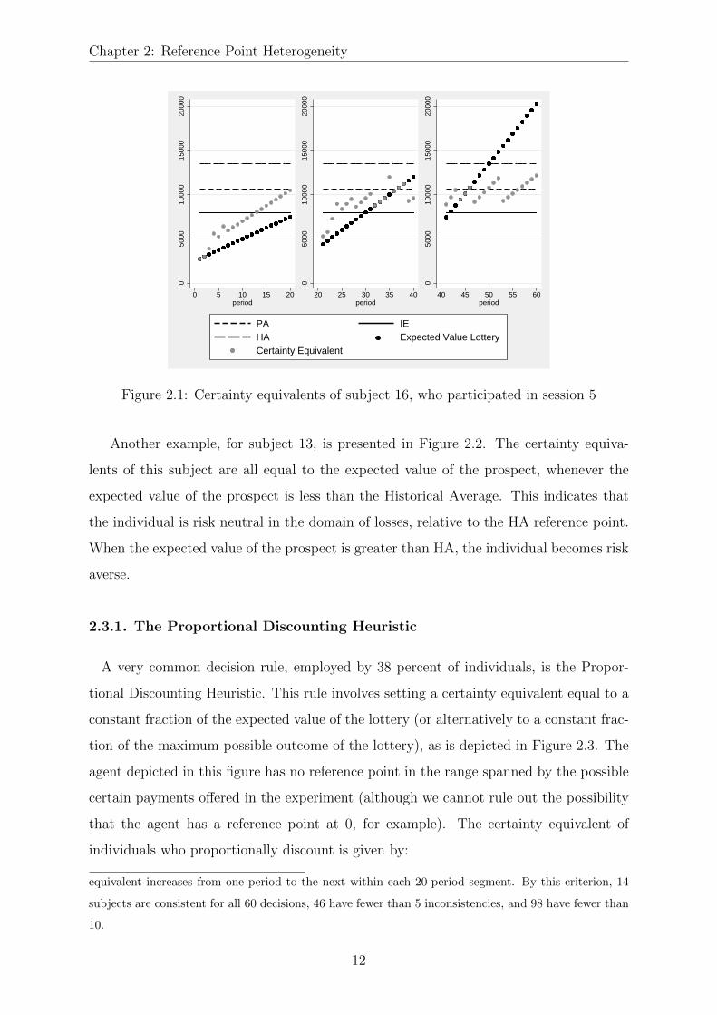
Figures 2.1 and 2.2 illustrate two of the typical decision profiles in our data. The
horizontal axis gives the period number, while the vertical axis shows monetary amounts
expressed in terms of experimental currency. The points displayed in black are the
expected values of the prospects presented in the period indicated. The certainty equiv-
alents elicited from the subject in the period are given by the grey points. The leftmost
panel shows the expected values of the prospects and the certainty equivalents elicited
in the first twenty periods. The expected values of these prospects include values both
above and below a candidate reference level. The figure shows that the certainty equiv-
alents of subject 16, who is depicted in the figure, are greater than the expected value of
the prospects, whenever the expected value lies in the domain of losses relative to the PA
reference point. Thus, the subject exhibits risk seeking behavior in this domain. When
the expected value of the lottery lies above the PA, the observed certainty equivalents
are less than the expected value of the prospects, which is consistent with risk averse
preferences. Thus, we observe here that the subject changes her attitude towards risk at
the PA payoff level.3
3One measure of consistency of choices that can be applied to the data is whether subjects’ certainty
10

Results
Tab
le2.
1:P
aram
eter
suse
din
the
exp
erim
ent
Ses
sion
Exp
ecta
tion
ofH
isto
rica
lE
xp
ecta
tion
of
Popu
lati
on
Exch
an
ge
Tre
atm
ent
Ow
nE
arnin
gs(I
E)
Ave
rage
(HA
)P
eers
(PE
)A
ver
age
(PA
)R
ate
1*35
00-6
500
5500
-8500
--
9100-1
2100
1300
Base
line
2-3
4500
-700
070
00-9
500
15600
-8600-1
1100
1300
Base
line
4-5
4500
-700
070
00-9
500
13500
-8600-1
1100
1300
Base
line
6-7
4500
-700
070
00-9
500
12700
-8600-1
1100
1300
Base
line
8-10
8500
-105
0015
500-
17000
13100
-7500-9
500
1500
Base
line
13-2
435
000-
4500
045
000-
60000
28500
-33000-4
3000
6500
Base
line
25-3
250
000-
6000
070
000-
85000
-100000
42000-5
2000
8500
Shif
t
33-4
450
000-
6000
070
000-
85000
-100000
48000-5
8000
9000
Shif
t
*Ses
sion
1is
excl
uded
from
the
anal
yse
sdu
eto
the
abse
nce
of
ahis
tori
cal
pee
rav
erage.
IEis
the
earn
ings
leve
lth
at
the
exp
erim
ente
rin
dic
ate
sto
ind
ivid
ual
that
isex
pec
ted
ofh
er.
PE
isth
eea
rnin
gsle
vel
that
the
exp
erim
ente
rin
dic
ate
sth
at
he/
she
exp
ects
oth
ers
part
icip
ati
ng
inth
esa
me
sess
ion
toea
rn.
HA
is
the
aver
age
earn
ings
ofin
div
idu
als
inal
lpri
orse
ssio
ns.
PA
is12
Eu
ros,
the
aver
age
earn
ings
inall
exp
erim
enta
lst
udie
sco
ndu
cted
at
the
lab
ora
tory
,m
inus
the
init
ial
endow
men
t.A
llre
fere
nce
poi
nts
are
sim
ilar
lyex
pre
ssed
net
of
init
ial
end
owm
ent
and
inco
me
shock
.W
ithin
ase
ssio
ndiff
eren
tin
div
iduals
had
diff
eren
tin
itia
lbal
ance
s,IE
and
PA
refe
ren
cep
oints
.T
hu
sth
ein
dic
ate
dva
lues
are
ranges
.H
owev
erea
chin
div
idual
him
self
had
au
niq
ue
init
ial
bala
nce
,IE
and
PA
leve
l.
11
Chapter 2: Reference Point Heterogeneity
050
0010
000
1500
020
000
0 5 10 15 20period
050
0010
000
1500
020
000
20 25 30 35 40period
050
0010
000
1500
020
000
40 45 50 55 60period
PA IEHA Expected Value LotteryCertainty Equivalent
Figure 2.1: Certainty equivalents of subject 16, who participated in session 5
Another example, for subject 13, is presented in Figure 2.2. The certainty equiva-
lents of this subject are all equal to the expected value of the prospect, whenever the
expected value of the prospect is less than the Historical Average. This indicates that
the individual is risk neutral in the domain of losses, relative to the HA reference point.
When the expected value of the prospect is greater than HA, the individual becomes risk
averse.
2.3.1. The Proportional Discounting Heuristic
A very common decision rule, employed by 38 percent of individuals, is the Propor-
tional Discounting Heuristic. This rule involves setting a certainty equivalent equal to a
constant fraction of the expected value of the lottery (or alternatively to a constant frac-
tion of the maximum possible outcome of the lottery), as is depicted in Figure 2.3. The
agent depicted in this figure has no reference point in the range spanned by the possible
certain payments offered in the experiment (although we cannot rule out the possibility
that the agent has a reference point at 0, for example). The certainty equivalent of
individuals who proportionally discount is given by:
equivalent increases from one period to the next within each 20-period segment. By this criterion, 14
subjects are consistent for all 60 decisions, 46 have fewer than 5 inconsistencies, and 98 have fewer than
10.
12

Results
5000
1000
015
000
2000
0
0 5 10 15 20period
5000
1000
015
000
2000
020 25 30 35 40
period
5000
1000
015
000
2000
0
40 45 50 55 60period
PA IEHA Expected Value LotteryCertainty Equivalent
Figure 2.2: Certainty equivalents of subject 13, who participated in session 3
Certainty equivalent = α ∗ Expected value of lottery = α ∗ yt/2 (2.1)
If α = 1, the individual is risk neutral. Another heuristic which is observationally
equivalent is the rule that Certainty equivalent = θ ∗ yt, where θ = α/2. Our setting
is conducive to observing the proportional discounting heuristic, because of the price
list format and the sequence of presentation of the choices. This is because if a subject
switches from the safe choice xjt to the risky choice yt at the same row on the table
in all periods, his behavior is consistent with the heuristic. Thus, an individual who
wishes to apply the heuristic would not find it excessively cognitively demanding to do
so. The average α parameter for this subsample is 0.92, equalling 0.96 for male and 0.90
for female subjects.
It is possible, if individuals have reference-dependent preferences, that α can differ
between the domains of losses and gains, as proposed by (Iturbe-Ormaetxe et al., 2011),
(Iturbe-Ormaetxe Kortajarene et al., 2015). Such a shift in the discount proportion
can be seen in the right panel of Figure 2.2. This behavior reveals a discrete change in
attitude toward risk above vs. below the reference point. However, in data such as ours,
a classification of individuals according to the behavioral rules they employ, such as the
Proportional Discounting Heuristic, must allow for some trials to exhibit deviations from
13

Chapter 2: Reference Point Heterogeneity
050
000
1000
0015
0000
0 5 10 15 20period
050
000
1000
0015
0000
20 25 30 35 40period
050
000
1000
0015
0000
40 45 50 55 60period
PA IEPE Expected Value LotteryCertainty Equivalent
Figure 2.3: Certainty equivalents of subject 100, who participated in session 32 and did
not employ a reference point
the exact decision consistent with the heuristic. To classify individuals as users of the
Proportional Discounting Heuristic, we calculate the following:
∆ proportional valuation = (certainty equivalent/expected value lottery)t - (certainty
equivalent/expected value lottery)t−1
x∗jt/(.5 ∗ yt)− x∗j,t−1/(.5 ∗ yt−1), x∗jt = minj{xjt|xjt < 0.5 ∗ yt} (2.2)
If the agent uses the proportional valuation heuristic, valuing every lottery at the same
constant fraction of its expected value, then ∆ proportional valuation always equals zero.
We classify an individual as a proportional discounter if she exhibits no more than six
instances over the 60-period session, in which equation (2) does not equal 0. Figure 2.4
illustrates the stability of the strategy employed on the part of users of the heuristic.
The figure is a histogram of (∆ proportional valuation) for the 38 percent of the sample
that are proportional discounters. The change in proportional valuation is zero in the
great majority of cases.
2.3.2. Reference points employed
To identify the reference points subjects are using, we focus on the manner whereby
a reference point influences decisions. A reference level is an important input for the
preference between receiving a certain amount or playing the gamble. When individuals
14

Results
05
1015
2025
Den
sity
−.5 0 .5 1
Change in discount proportion
Figure 2.4: Density of changes in discount proportion parameter α between periods t
and t+1
Table 2.2: Example of choices when the reference level equals 90
Lottery Outcome Expected Value Certain Amount Choice
.5*240 120 48 Lottery
.5*240 120 72 Lottery
.5*240 120 96 Certain Amount
.5*240 120 120 Certain Amount
.5*240 120 144 Certain Amount
.5*240 120 168 Certain Amount
.5*240 120 192 Certain Amount
.5*240 120 216 Certain Amount
have to choose between a prospect and a certain amount, this choice will depend on
whether the individual can receive his reference level by accepting the certain amount. If
not, the individual will prefer playing the lottery and aiming for a favorable outcome in
order to reach his reference payoff level. On page 273 of Prospect Theory, (Kahneman and
Tversky, 1979) point out that the certainty of receiving one’s reference level will always
be preferred to playing a prospect with equal expected value, given that an individual is
risk averse.
Hypothesis 1: When the certain amount offered exceeds the reference level of an
individual, the certain amount will be preferred to playing the gamble.
We test for the presence of a target payoff level by investigating the choice between
playing the lottery and receiving the certain payment. Therefore, we expect that a refer-
15

Chapter 2: Reference Point Heterogeneity
ence point will influence decisions when the certain payment is just above the reference
level. In such cases, risk averse agents might forego some expected payoff and choose the
certain payment, in order to reach their reference payoff with certainty. Depending on
the risk aversion level of the individual, the certain amount will be preferred to gambles
with an expected value higher than the reference point. For our analysis this results in
the following predictions; if the certain amount offered is less than the reference point
of the individual, then the gamble will be preferred. On the other hand, whenever the
certain amount is equal or larger than the reference point, the individual will prefer the
certain amount offered and will forego some expected value of the gamble. Table 2.2
provides an illustrative example of a hypothetical subject.
To test for this pattern, we model the choice between the certainty equivalent and
the lottery of each individual as a function of the value of the certainty equivalent, the
expected value of the lottery and a dummy variable indicating whether the safe option
xjt exceeds the reference point.
Zijt = αi + β1,i.5 ∗ yt + β2,ixjt + γkDk + ε (2.3)
where
Dk =
1; if Certain amount > reference point k
0; if Certain amount ≤ reference point k
Zijt is a binary variable which represents the choice of individual i between the
prospect (.5, yt), and the certain amount on offer, xjt4 , in period t. Zijt takes the value
1 if the individual chooses the prospect, and 0 otherwise. Recall that all reference points
are net of the initial endowment. A significant coefficient for the γk term would indicate
the use of reference point k, as it reveals a change in the likelihood of choosing the lottery
when the certain payment it is paired with exceeds the reference level. In the regression,
we control for the expected value of the lottery and the level of the certain payment.
The model is estimated for each individual i and each reference point k separately. An
F-test is performed to test for the significance of the restriction Dk = 0. If the resulting
F-statistic is above the critical level, and the estimated gamma coefficient is negative,
4the correlation between xjt and (.5, yt) ranges between 0.67 and 0.76, which seems to be in an
acceptable range
16

Results
we will say that k is a reference point for the individual. When this test is significant for
candidate reference point k, we say that the individual is using k as a reference point.5
Based on the result of this test, we assign an individual to either none, one, or multiple
reference points. For each individual, the regression is estimated for each of the potential
reference points. Table 2.1 shows the incidence of each possible reference point profile in
the sample.
The table shows that the PA is the most common reference point for individuals who
used only one reference level, followed by IE and HA. PE does not seem to serve as a
reference point. A sizable portion of subjects use multiple reference points, and most of
these individuals use PA paired with HA. Lastly, a non-negligible portion of individuals
do not appear to employ any of the candidate reference points. Gender differences are
not significant, with Fisher exacts tests resulting in p-values of .61 for sessions 2 - 24,
and .097 for sessions 25 - 44.
Regressions with the specification in 2.3 on the aggregate pooled data from all indi-
viduals classified as using each reference point provide an overall picture of the estimated
parameters, and of the strength of the attraction of each reference point. Recall that
each reference point, other than PA, is specified as in addition to the initial endowment.
The estimates are shown in Tables 2.4 and 2.5. The results show that an increase in
the expected value of the lottery increases the probability of choosing the lottery. On
the other hand, increasing the value of the certain alternative decreases the probability
of choosing the lottery. Each of the reference points is negative and significant in both
tables. This indicates that for each of the reference points PA, HA, and IE, a subset
of subjects exhibits changes in behavior for payoff levels above vs. below the reference
point. When the certain payoff exceeds the reference point, it is more likely to be chosen.
2.3.3. Income shock
In the Shift treatment, we study the effect of a shock to an individual’s income level and
investigate whether it changes the likelihood of choosing a particular reference point. In
this treatment, at the end of period 40, subjects experience a change in their wealth. We
increase their cash balance by fifty percent of their initial endowment, an amount which
differs among subjects. Then, in the last 20 periods of the session, the same set of choices
58 percent of the subjects exhibited a positive gamma
17

Chapter 2: Reference Point Heterogeneity
Table 2.3: Reference point use by subjects
Session All sample Female Male*
2-24
None 17.83% 16.66% 20.57%
Population Average (PA) 15.05% 23.29% 10.26%
Individual Expectation (IE) 21.93% 26.69% 20.52%
Historical Average (HA) 8.23% 6.69% 7.69%
PA and IE 2.75% 3.34% 2.58%
PA and HA 34.21% 23.34% 38.39%
IE and HA 0% 0% 0%
All 0% 0% 0%
25-44
None 26.61% 37.42% 17.79%
Population Average (PA) 62.27% 52.53% 73.38%
Individual Expectation (IE) 2.23% 0% 2.23%
Peer Expectation (PE) 0% 0% 0%
PA and IE 8.88% 10.05% 6.61%
PA and PE 0% 0% 0%
IE and PE 0% 0% 0%
All 0% 0% 0%
The gender variable contains 5 missing values.
18

Results
Table 2.4: Estimated effect of reference point in sessions 2 - 24
(1) (2) (3)
choice choice choice
EV Lottery (.5 ∗ yt) 0.05∗∗∗ 0.09∗∗∗ 0.06∗∗∗
(7.48) (14.04) (10.39)
xjt -0.05∗∗∗ -0.07∗∗∗ -0.06∗∗∗
(-9.55) (-16.09) (-13.61)
DPA -0.42∗∗∗
(-16.01)
DIE -0.37∗∗∗
(-15.69)
DHA -0.35∗∗∗
(-11.04)
Gender -0.05 -0.02 -0.03
(-1.51) (-0.54) (-0.84)
Constant 0.61∗∗∗ 0.49∗∗∗ 0.64∗∗∗
(19.95) (13.65) (18.02)
Observations 16720 8616 12896
R2 0.514 0.544 0.538
t statistics in parentheses
Robust standard errors
∗ p < 0.1, ∗∗ p < 0.05, ∗∗∗ p < 0.01
19

Chapter 2: Reference Point Heterogeneity
Table 2.5: Estimated effect of reference point in sessions 25-44
(1) (2)
choice choice
(1) (2)
choice choice
EV Lottery (.5 ∗ yt) 0.06∗∗∗ 0.07∗∗∗
(11.63) (11.00)
xjt -0.05∗∗∗ -0.05∗∗∗
(-13.85) (-14.01)
DPA -0.46∗∗∗
(-26.64)
DIE -0.33∗∗∗
(-16.01)
Gender 0.02 -0.01
(0.81) (-0.32)
Constant 0.56∗∗∗ 0.43∗∗∗
(22.18) (9.91)
Observations 29192 3824
R2 0.552 0.579
t statistics in parentheses
Robust standard errors
∗ p < 0.1, ∗∗ p < 0.05, ∗∗∗ p < 0.01
20

Results
Table 2.6: Reference points of subjects in Shift treatment before and after the income
shock
Period 1-20 Period 41-60
None 36.07% 41.00%
Population Average (PA) 59.00% 57.35%
Individual Expectation (IE) 1.64% 0%
Peer Expectation (PE) 3.29% 0%
PA and IE 0% 0%
PA and PE 0% 0%
IE and PE 0% 1.64%
All 0% 0%
as in the first 20 periods are presented to the subjects again. We consider the effect of
the shock on the choices of individuals in the last twenty periods of the experiment and
compare these to the choices elicited in the first segment of twenty periods, with respect
to which reference points most accurately characterize the decision pattern. Shocking
the initial balance level creates a restart and provides a shock to incentives. By doing
so, we are able to investigate whether experience affects the employed reference point.
This would also indicate if reference points are easily adapted and how sticky they are.
We expect that the employed reference points will not show any difference.
We report the proportions of reference points that fit best the decisions of these
individuals in Table 2.6. The first column reports a classification of individuals in relation
to reference points in periods 1 - 20 in the Shift treatment. The second column contains
analogous data from periods 41 - 60. The results show no significant difference in the
incidence of the use of each reference point before, compared to after, the shock. A
Fisher exact test of the equality of the distribution of reference points between periods 1
- 20 and 41 - 60 results in p = 0.481. This may reflect the fact that the shock, like initial
income, is treated as a separate source of wealth than the earnings from the experimental
task.
21

Chapter 2: Reference Point Heterogeneity
2.4. Discussion
In this paper, we document heterogeneity among individuals in their personal inclination
to use particular reference points. It is known from previous work that the reference point
that characterizes a set of data best differs, depending on the setting in which the decision
is taking place. However, we show here that the reference point that best fits the decision
pattern of an individual also differs by individual, keeping the decision setting constant.
Our results do indicate that when individuals use a single reference point, the pop-
ulation average payoff level is the most frequently employed. This is followed by the
anticipated payoff level indicated for the individual, and in turn by the average that
comparable individuals have earned in past similar tasks. No participant used the earn-
ings of peers in the same session as a reference point. The results are similar for men and
women and we observe no significant gender differences in the use of reference points.
We also observe that a sizable fraction of individuals employs multiple reference
points. The most common combinations of reference points are the population average
with the historical average, and the population average with the individual expectation.
It is striking to us that PA is such a strong attractor, in light of the fact that the
social distance between an individual and the population average is arguably the greatest
among all of the reference points that we have considered. The experimental design we
have does not allow us to isolate the precise reason that PA is more prominent than
the others. However, it does have the feature that it, along with HA, is historical and
therefore certain, while IE and PE are anticipated future payoff levels. Furthermore,
PA is always constant and known to be the same for all individuals, while the three
other reference points can vary among individuals. Perhaps a reference payoff is more
compelling when it is common knowledge that it is the same for everyone.
We also find that a considerable share of subjects tend to proportionally discount their
certainty equivalent by a constant percentage of the expected payoff of the risky lottery.
Some of these individuals also discount by a different fraction, depending on whether
payoffs are above or below one or more of the reference points. The widespread use of
the Proportional Discounting Heuristic seems intuitive as a behavioral rule, because it is
simple to calculate and apply, though to our knowledge its use has not been documented
in previous research.
22

Appendix
Thus, our experiment illustrates two types of heterogeneity in how individuals per-
ceive risky decision making tasks. The first is that some individuals differ in whether or
not they apply a simple heuristic, proportional discounting, to value the lottery, while
others adopt more complex or inconsistent valuation methods. The second is that the
reference level of earnings that individuals use is idiosyncratic, with some individuals
targeting one or more from among a set of prominent reference points, while others do
not.
While most studies have focused on estimating the mean and median loss aversion
parameters of a particular sample, a growing number of studies have documented het-
erogeneity in the loss aversion level of individuals ((Fehr and Goette, 2007), (Gachter
et al., 2007), (Von Gaudecker et al., 2011)). Building on this, other studies have in-
vestigated factors affecting the degree of individual loss aversion and have found that
demographic characteristics play an important role ((Hjorth and Fosgerau, 2009), (Payne
et al., 2015)). Our results complement this line of research by providing evidence that
individuals exhibit different reference points in a similar task. This is important because
loss aversion only has meaning relative to a reference point.
2.5. Appendix
23

Chapter 2: Reference Point Heterogeneity
2.5.1. Instructions
This experiment is about decision making. The experiment consists of 60 periods. Each
period you will be presented a sequence of choices. The currency used in the experiment
is francs. The amounts which are presented to you are all in terms of francs. You will
be paid in cash in Euro’s according to your realized earnings by bank transfer the very
same day. The conversion rate is 8500 francs to 1 Euro. You start with an initial amount
of francs. The experimenter expects you to earn francs. The average amount
earned in this experiment by other participants is francs.
Each presented choice consists of two options. One option is a sure amount of
francs, the other option is a lottery with two possible outcomes. Each outcome of the
lottery has a probability of one half to be realized. This is true for all lotteries presented
to you throughout the experiment. In each period you have to indicate for each choice
whether you prefer the lottery of that period, as shown at the upper part of the screen,
or the certain amount of money. At the end of the experiment, the computer will
randomly select one period and one choice of that period to determine your earnings of
this experiment. Each period has equal probability of being selected by the computer and
each choice has equal probability of being be selected by the computer. Then, depending
on how you decided in the period and choice that counts, you either receive the sure
payment or the lottery.
You will start with an initial balance of francs. After you have finished the
experiment by indicating your choices, the outcome of the round which will be played
for real will be added to your initial earnings and this will become your final earning of
the experiment.
The experimenter expects that you will earn francs in this session. However,
please notice that the expectations of the experimenter are not driven by any knowledge
about the outcome.
THE NEXT PARAGRAPH WAS ONLY INCLUDED IN SESSIONS 1 - 24
Average earnings in previous sessions of this experiment have been francs.
However, conditions may be changed from session to session and average earnings may
be considerably different in this session from previous ones.
THE NEXT PARAGRAPH WAS ONLY INCLUDED IN SESSIONS 25 - 44
24

Appendix
The experimenter expects that other participants in this session will earn on average
francs. However, conditions may be changed from session to session and average earnings
may be considerably different in this session from previous ones.
25


Chapter 3
Reference Point Formation and
Demographics
3.1. Introduction
We differ in evaluating the outcome of a risky choice around a reference point, which
we use as a benchmark to evaluate our well-being. Reference dependent preferences,
which was pioneered by the work of (Kahneman and Tversky, 1979), have been widely
documented in decision making under risk. Experimental studies have demonstrated
the effect of reference point formation on effort provision ((Abeler et al., 2011)), the
pricing of securities ((Kahneman et al., 1991)) and consumer products ((Ericson and
Fuster, 2011)). Studies conducted with field data have presented evidence of reference
point formation in household saving, labor market participation, consumer behavior,
education, and investment decisions (e.g. (Camerer, 2004), (Starmer, 2000), (Grinblatt
and Han, 2005), (Hardie et al., 1993), (Camerer et al., 1997)).
The selection of a pay-off level as a reference point by an individual remains an
open question to be explored. In this study we investigate the exhibition of employing a
particular reference point when subjects face a risky decision making task in a decontex-
ualized setting among a demographically representative Dutch sample. We conducted an
experiment designed to investigate which of two competing reference points dominates
in a risky decision making task among a representative Dutch sample. The two reference
points are: (1) an earnings level that is expected by the experimenter for the individual,
(2) the expected average earnings level of peers. In the experiment, we elicit certainty
equivalents of a number of lotteries and obtain estimates of individual reference points.
The design permits detection of individuals who use no or one unique reference point.
Eliciting reference points in a decontextualized environment also eliminates potential
heterogeneity of using different sources for a peer group reference level depending on the
27

Chapter 3: Reference Point Formation and Demographics
domain of risky choice as different peer groups could be used as ones social comparison
level depending on the domain of choice under risk. As is shown in previous studies,
the social comparison benchmark could be in lateral, downward or upward direction.
A downward comparison level leads to a more favorable perception about one’s own
well-being and induces positive emotions (e.g., (Wood et al., 1985). On the contrary,
an upward social comparison level serves as a driver of improvement strivings ((Collins,
1996), (Helgeson and Mickelson, 1995) and (Taylor et al., 1995)). We find heterogeneity
in the reference point employed and correlation between certain demographic and per-
sonality traits and the employment of a reference point. The individual expected payoff
level and the expected payoff level of peers are equally likely to be employed as a refer-
ence level. Our results also show that the income level of an individual does not play a
role in the exhibiting the use of a payoff level as reference point. Our results are highly
relation to the study by (Baillon et al., 2015) who investigate a similar question. Their
study also shows that reference points are heterogeneous among individuals. However,
their study exploits different payoff levels which can serve as potential reference points.
With our experimental design we also rule out overlapping reference points since we test
for potential reference points which are all driven by expectations.
Reference points might differ depending on the domain of risky choice and have
been typically given as exogenous or defined for a particular situation in previous stud-
ies(Koszegi and Rabin, 2006). In providing evidence of reference point formation, the
reference points of the decision maker are in general taken as evident given the deci-
sion context. Expectation bases payoff levels are shown to be successful in serving as
a reference point. The expectation level of the individual have been modeled as a ref-
erence point in prominent theories of reference point formation ((Bell, 1985), (Loomes
and Sugden, 1986), (Koszegi and Rabin, 2006), (Koszegi and Rabin, 2007), (Heidhues
and Koszegi, 2008)). In empirical work, expectations-based reference points have been
able to explain insurance choices ((Barseghyan et al., 2011)), and labor supply decisions
((Farber, 2005), (Farber, 2008), (Crawford and Meng, 2011)). Another strong candi-
date which serves as a reference level is the social peer group payoff level ((Gali, 1994),
(Abel, 1990), (Vendrik and Woltjer, 2007), (Linde and Sonnemans, 2012)). Experimental
studies have mainly supported the models of inequity aversion proposed by (Fehr and
Schmidt, 1999) and (Bolton and Ockenfels, 2000), in which the average payoff of peers
28
Introduction
serve as a reference point. In a decontextualized risky lottery choice experiment, we test
for the inclination to choose between the individual expectation level and or an expected
payoff level of a social peer group and investigate which demographic and personality
traits determine the choice of reference point.
Our study imposes different initial income levels to subjects without informing
subjects about any differences in the status quo level between subjects. This allows us to
test for the effect of an initial endowment on the likelihood of targeting a reference point
and if targeted, the employment of a reference point based on peer group expectation or
a more internally driven expectation about one’s own earnings. (Ordonez et al., 2000)
focuses on differences in status quo levels between the individual and a peer group in a
hypothetical choice experiment and find that differences between the status quo level of
the individual and the peer group had significant impact on their pay satisfaction. They
also show that this effect is asymmetric i.a. having a higher status quo level than the
peer group produced weaker positive satisfaction. (Masatlioglu and Ok, 2005) model the
theory of choice in a static setting where the initial endowment or status quo plays a
key role. They show that the reference dependent agent prefers to stay at his status quo
as long as another option is not better in all dimensions from his current endowment.
Terzi et al (2015) demonstrates that changing income levels do not change the reference
point employed by the subject at the outset of the experiment. By varying the initial
endowment provided to subjects without informing them about the initial endowment of
peers, we can analyze any income effect on reference point employment where the initial
endowment to peers cannot affect the employed reference point as in (Ordonez et al.,
2000). Our study finds that the a higher initial endowment level at the outset of the
experiment has a positive effect on exhibiting the use of a reference point but does not
affect the use of a particular payoff level as a reference point.
We also explore the correlates of personality traits and the employment of reference
points. Previous literature has documented several relationships between personality
dimensions and economic outcomes or preferences, including the accumulation of wealth
((DeNeve and Cooper, 1998), (Steel et al., 2008), (Ameriks et al., 2007)), wages ((Mueller
and Plug, 2006)), and risk preferences ((Borghans et al., 2009)). Various studies tried to
identify economic mechanisms associated with the big five personality traits ((Denissen
and Penke, 2008), (DeYoung et al., 2010), (Van Egeren, 2009)). They documented that
29

Chapter 3: Reference Point Formation and Demographics
extraversion relates to responsiveness to reward and incentives. Neuroticism mainly
concerns the feeling of threat and punishment. Agreeableness is reflected in the affinity
toward altruism and cooperation. Conscientiousness results in controlled behavior and
goals and openness originates in the high utilization and absorption of information. Our
results show that personality traits seem to have a considerable effect on the formation
and the selection of a particular reference point. We find that individuals who score
high on neuroticism are less likely to form a reference point. Additionally, we find strong
correlation between extraversion and the selection of a payoff level as a reference point.
Extravert individuals are more inclined to use the peer group average as their reference
levels.
The remainder of this paper is organized as follows. Section 3.2 will describe the
subject pool and experimental design. In Section 3.3 we will discuss the results on the
prevalence of reference point employment among the sample and the correlation between
demographic and personality traits and Section 3.4 will conclude.
3.2. Experiment
3.2.1. Design
The experiment consisted of 20 periods, in which subjects are presented with a binary
prospect (1/2, yt) which results in outcome yt with probability .5 and in outcome 0 with
probability .5. The probability p is set to equal to 0.5 throughout the experiment. This
feature allows us to sidestep the issue of probability weighting. This prospect is paired
with eight different certain payment levels, xjt, j = 1, ..., 8 in a price list format. In each
period, each subject is asked to make eight choices. Each choice in period t is between
(1/2, yt) and xjt. The eight choices are displayed on the subject’s computer screen
simultaneously. The magnitude of xjt ranges in value from 20 percent to 140 percent
of yt/2, the expected value of the prospect. The certain payments appear in ascending
order of magnitude in the price list on the computer screen. Participants face 8 questions
per period which adds up to a total of 160 questions. The main advantage of using a
multiple price list format to elicit risk preferences is that it is relatively transparent and
easy to understand to subjects and provides simple incentives for truthful revelation. On
30

Experiment
the other hand, the main disadvantage is potential susceptibility to framing effects as
revealed preferences might be sensitive to procedures, subject pools, and the format of
the multiple price list table (Andersen et al., 2006). However, their results show that the
general finding of risk aversion by subjects is robust. In addition, (Charness et al., 2013)
show that the multiple price list format is good in capturing differences in individual risk
preferences and that elicited preferences through this method have also been shown to
correlate with other individual characteristics and real world risk-taking behavior.6.
The binary prospect (.5, yt) increases in constant increments from one period to
the next. The lowest certain amount xjt chosen by the subject over (.5, yt) in period t,
serves as our measure of the certainty equivalent for the prospect (.5, yt) for that subject.
The expected value of the prospects and the potential certainty equivalents span the two
potential reference points. Thus, the expected values of (.5, yt), as well as the value of xjt,
are in some instances in the domain of gains and at other times in the domain of losses
relative to each of the two reference points we consider. When the expected value of the
prospect lies below a particular reference points, this domain will form the loss domain
that belongs to this particular reference point. The expected value of the subsequently
presented prospects will exceed the value of the reference point. Thus, these prospects
lie in the mixed domain of gains and losses.
At the start of the experiment each subject was given information about their initial
balance, which was a lump sum payment. Next to this information, we provided subjects
with the expectation of the experimenter about the individual earnings of the subject
(IE) and the expectation of the experimenter about the earnings of peers participating at
the same experiment (PE). While both potential reference levels rely on an expectation
level, the orientation of the payoff levels differ. The first statement focused on an internal
expectation level, whereas the latter concerned a peer group expectation. By having
both potential reference points depending on an expectation level of the experimenter
we can rule out overlapping expectation based reference levels. I.e. an individual could
extrapolate that the peer group expected earning is a good indicator of his/her own
expected earning. If this is the case, expected individual earnings and expected peer
6We don’t think that switching in the middle is driven by a bias as only 15 percent switch in the
middle. Given the overall distribution of choices, there does not seem to be a specific spike about he
middle. y, having 15 percent of the switches in the middle does not create a suspicion of a bias.
31

Chapter 3: Reference Point Formation and Demographics
Table 3.1: Parameters used in the experiment
Subsample Initial Balance IE PE Shock
1 20 30 40 Yes
2 20 40 30 No
3 30 20 40 No
4 30 40 20 No
5 40 30 20 No
6 40 20 30 No
earnings would coincide, see (Koszegi and Rabin, 2006). The two candidate reference
points were also available on the subjects’ screen during the course of the experiment.
We varied the magnitudes of the initial balance level and the two reference points
in different treatments. These values are shown in Table 3.1. The first column of Table
3.1 indicates the subsample, and each row groups together the sample conducted under
identical parameters. Column 2 shows the initial balance level which is provided to
subjects and could be considered as a minimum income level. Columns 2-4 contain the
monetary values of each of the candidate reference points.
The levels of the potential reference points varied for different subsamples in order
to identify the employment of a reference point while controlling for the relative position
w.r.t the other reference point. The parameters for each subsample are shown in Table
3.1. Payoffs are denominated in Euros. To identify the selection of a certain reference
point regardless of its’ relative position, we vary the magnitude of the reference points by
assigning different payoff levels to the potential reference points for different subsamples.
This design allows the hypotheses that individuals have a tendency to use the highest
or lowest from the set of plausible reference points to be evaluated. We also varied the
level of initial balance in order to investigate the effect of different lump sum payments
at the outset of a decision task on the employment of reference points.
3.2.2. Hypothesis
To identify the reference points subjects are using, we focus on the manner whereby
a reference point influences decisions. A reference level is an important input for the
preference between receiving a certain amount or playing the gamble. When individuals
32

Experiment
have to choose between a prospect and a certain amount, this choice will depend on
whether the individual can receive his reference level by accepting the certain amount. If
not, the individual will prefer playing the lottery and aiming for a favorable outcome in
order to reach his reference payoff level. On page 273 of Prospect Theory, (Kahneman and
Tversky, 1979) point out that the certainty of receiving one’s reference level will always
be preferred to playing a prospect with equal expected value, given that an individual is
risk averse.
Hypothesis 1: When the certain amount offered exceeds the reference level of an
individual, the certain amount will be preferred to playing the gamble.
We test for the presence of a target payoff level by investigating the choice between
playing the lottery and receiving the certain payment. Therefore, we expect that a refer-
ence point will influence decisions when the certain payment is just above the reference
level. In such cases, risk averse agents might forego some expected payoff and choose the
certain payment, in order to reach their reference payoff with certainty. Depending on
the risk aversion level of the individual, the certain amount will be preferred to gambles
with an expected value higher than the reference point. For our analysis this results in
the following predictions; if the certain amount offered is less than the reference point
of the individual, then the gamble will be preferred. On the other hand, whenever the
certain amount is equal or larger than the reference point, the individual will prefer the
certain amount offered and will forego some expected value of the gamble.
3.2.3. Procedure
The computerized experiment was conducted online using the Center Panel managed by
CentERdata. We randomly invited a subsample from this panel to participate at our ex-
periment. In total, 1056 individuals who were member of the Center Panel participated
in the experiment. The experiment was incentivised, next to a yearly payment which
members receive for participating regularly in surveys. A large number of demographic
variables of these respondents are available which were collected at earlier surveys. Next
to the socio-economic background variables, we matched our sample with personality
data on the Big Five Personality Factors. This data of the individuals is collected by the
Dutch Household Panel, which is also managed by CentERdata. Both panels contain a
representative sample of the Dutch population in terms of observable background char-
33

Chapter 3: Reference Point Formation and Demographics
acteristics of respondents. Our matched dataset includes a large number of demographic
variables and data on the big five personality traits. 10 percent of the revealed preferences
was inconsistent and therefore deleted for the analysis. We found correlation between
the number of inconsistent revealed preferences and demographic factors. Namely, men
were less likely to provide inconsistent preferences. The age of an individuals seemed
to correlate with inconsistent preferences with a correlation coefficient of .27. Income
and eduction level correlated negatively with the number of inconsistent answers with a
correlation of -.05 and -.11 respectively.
The experiment had real incentives as 10 percent of the respondents were paid out
their earnings of the online experiment. The earnings of the participants were randomly
determined by the computer at the end of the experiment. The computer chose one
period and one of the decisions of that period to determine each subject’s earnings.
Depending on the choice of the subject, the subject either played the lottery and received
the outcome of the prospect or received the certain amount.7
3.3. Results
To elicit the reference point subjects employed in the experiment, we focus on the pref-
erence of subjects between playing the lottery or accepting the certain amount offered.
We test for the presence of a target payoff level by investigating the choice between
playing the lottery and receiving the certain payment. We expect that the presence of a
reference point will influence decisions when the certain payment is just above the ref-
erence level. In such cases, depending on the loss aversion of the agent he might forego
some expected payoff and choose the certain payment, in order to reach his reference
payoff. To test for this pattern, we model the choice between the certainty equivalent and
the lottery of each individual as a function of the value of the certainty equivalent, the
expected value of the lottery and a dummy variable indicating whether the safe option
xjt exceeds the reference point.
Zijt = αi + β1,i.5 ∗ yt + β2,ixjt + γkDk + ε (3.1)
7This procedure removes wealth effects. Starmer and Sugden (1991) have shown that this procedure
is successful in revealing the monetary preferences of subjects under uncertainty.
34

Results
where
Dk =
1; if Certain amount > reference point k
0; if Certain amount ≤ reference point k
Zijt is a binary variable which represents the choice of individual i between the
prospect (.5, yt), and the certain amount on offer, xjt, in period t. Zijt takes the value
1 if the individual chooses the prospect, and 0 otherwise. A negative and significant
coefficient for the γk term would indicate the use of reference point k89, as it reveals a
change in the likelihood of choosing the lottery when the certain payment it is paired
with exceeds the reference level. In the regression, we control for the expected value of
the lottery and the level of the certain payment.
The model is estimated for each individual i and each reference point k separately.
When the estimated gamma coefficient is negative and significant for candidate reference
point k, while also having the highest absolute value among the two estimated gamma
terms we will say that k is a reference point for the individual. Based on the result of this
test, we assign an individual to either the reference level based on the individual expected
payoff level or the expected payoff level of peers. We have chosen for a conservative
approach in which we did not allow for the probability of multiple reference points.
Given that we have 20 observations per subject, we focused on the best fitting potential
reference point. Table 3.2 shows the incidence of each possible reference point profile in
the sample.
Both candidate reference points seem to be equally prominent in serving as a
reference level. We find a small difference in the utilization of reference points when we
split the sample according to gender. However, inspecting differences in reference point
formation between younger and older individuals shows that older individuals are more
likely to use the social comparison level. However this difference is not significant given
a P-value of .831 of a KS-test.
Regressions with the specification in 3.1 on the aggregate pooled data from all
individuals classified as using no reference point, IE or PE provide an overall picture of
8the correlation between xjt and Dk lies between 0.59 an 0.72 depending on the reference level, which
is within acceptable range911 percent of the individuals have exhibited a positive γk
35

Chapter 3: Reference Point Formation and Demographics
Table 3.2: Reference points employed by subjects
No reference point Individual Expectation (IE) Peer Expectation (PE)
Full sample 61.72% 19.71% 18.57%
Female subsample 59.87% 19.53% 20.60%
Male subsample 63.45% 19.88% 16.67%
Age<40 60.12% 23.68% 16.20%
Age=>40 62.52% 17.73% 19.75%
the estimated parameters, and of the strength of the attraction of each reference point.
The estimates are shown in Table 3.3. The results show that an increase in the expected
value of the lottery increases the probability of choosing the lottery. On the other hand,
increasing the value of the certain alternative decreases the probability of choosing the
lottery. Each of the reference points is negative and significant in both tables. This
indicates that for each of the reference points a subset of subjects exhibits changes in
behavior for payoff levels above vs. below the reference point. When the certain payoff
exceeds the reference point, it is more likely to be chosen.
3.3.1. Reference point formation, demographics and personality
Personality variables
As a measure of personality, we use the Big Five Factor model. This is the most
widely used concept to describe personality condensed in big five traits, namely con-
scientiousness (C), openness (O), agreeableness (A), neuroticism (N) and extraversion
(E). Most personality dimensions can be extracted from this model. These factors can
be described as follows: Conscientiousness focuses on self-discipline, planning, organized
behavior, and carefulness, whereas the opposite includes laziness, less goal oriented and
unreliable. Openness encloses high fantasy levels, intellectual curiosity, openness to new
experiences versus being rational, conventional and practical. Agreeable individuals are
soft-hearted, trusting, cooperative and helpful versus ruthless, disagreeable and aggres-
sive. Neuroticism includes anxiety, insecurity, nervousness, depressions and moodiness as
opposed to emotional stability, being calm and self-confident. Extraversion encompasses
36

Results
Table 3.3: Properties of preferences
(NO) (IE) (PE)
EV Lottery (.5 ∗ yt) 0.0087∗∗∗ 0.0095∗∗∗ 0.0098∗∗∗
(20.92) (15.38) (15.30)
xjt -0.0148∗∗∗ -0.0102∗∗∗ -0.0107∗∗∗
(-29.92) (-13.29) (-12.34)
DIE -0.5485∗∗∗
(-27.08)
DPE -0.5181∗∗∗
(-24.68)
Constant 1.6373∗∗∗ 1.6883∗∗∗ 1.6722∗∗∗
(119.38) (90.57) (91.99)
Observations 95984 30198 28371
R2 0.153 0.529 0.506
C olumn 1 includes data on individuals who did not
form a reference level. Column 2 and 3 include obser-
vations of subject who have based their reference levels
on IE or PE respectively. t statistics in parentheses. *
p < 0.1, ** p < 0.05, *** p < 0.01. Robust standard
errors clustered at subject level.
37

Chapter 3: Reference Point Formation and Demographics
sociability and assertiveness, attention versus reservation and timidity. Using the first
principal component extracted by applying a Principal Component analysis, we condense
the self-reported responses of individuals to various questions related to each personal-
ity trait to one score level per personality trait. This principal component is used to
determine the score of an individual on a specific personality trait.
After determining the incidence of reference point formation and selection of a par-
ticular payoff level as a reference point, we investigate demographic factors and person-
ality traits containing explanatory power in using a payoff level as a reference point. We
investigate the correlates between the inclination of exhibiting a reference level and the
demographic and personality traits of an individual using a Logit estimation. Our depen-
dent variable equals 1 if the individual has employed a reference point in the decision mak-
ing task, and 0 otherwise. Several demographic variables Wd, d = Income,Age,Gender
and the big five personality factors Pb, b = A,O,E,N,C are considered. We also include
a variable on self esteem levels. Lastly, we include a variable on the initial balance to
test for wealth effects. Table 3.4 presents the results of this specification. We observe
that neurotic individuals are less likely to employ a reference level. An increase in the
income level of an individual increases the likelihood that an individual employs a ref-
erence level. This shows that initial endowment levels do change incentives and have an
effect on targeting a payoff level as a reference point. This effect might be driven by
optimisim created by a higher initial wealth level.
Z = α + βwwi + βPbPbi+ βIBIBi + ε (3.2)
Furthermore, we asses the employment of a particular payoff level as a reference
point. We restrict our sample to individuals who have employed a reference level. Using
a similar approach as specification 3.1 we investigate the inclination of exhibiting a
particular reference level. Our dependent variable takes on a value of 0 if the individual
has employed the individual expectation level as a reference point, and 1 if the individual
has employed the expected average peer earnings as a reference level. Table 3.5 shows the
results of the specification explaining the employment of a particular reference level as a
function of demographic factors and personality traits. We observe that older individuals
are more likely to employ a peer group average earning level as their reference point. The
initial balance level given at the start of the experiment does not contain explanatory
38
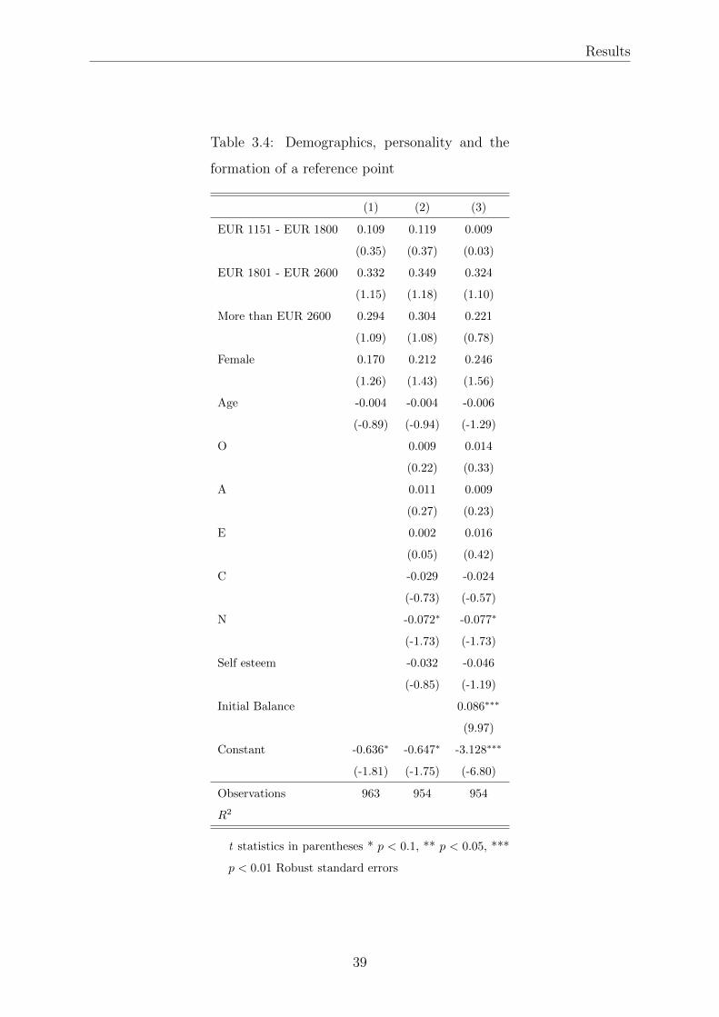
Results
Table 3.4: Demographics, personality and the
formation of a reference point
(1) (2) (3)
EUR 1151 - EUR 1800 0.109 0.119 0.009
(0.35) (0.37) (0.03)
EUR 1801 - EUR 2600 0.332 0.349 0.324
(1.15) (1.18) (1.10)
More than EUR 2600 0.294 0.304 0.221
(1.09) (1.08) (0.78)
Female 0.170 0.212 0.246
(1.26) (1.43) (1.56)
Age -0.004 -0.004 -0.006
(-0.89) (-0.94) (-1.29)
O 0.009 0.014
(0.22) (0.33)
A 0.011 0.009
(0.27) (0.23)
E 0.002 0.016
(0.05) (0.42)
C -0.029 -0.024
(-0.73) (-0.57)
N -0.072∗ -0.077∗
(-1.73) (-1.73)
Self esteem -0.032 -0.046
(-0.85) (-1.19)
Initial Balance 0.086∗∗∗
(9.97)
Constant -0.636∗ -0.647∗ -3.128∗∗∗
(-1.81) (-1.75) (-6.80)
Observations 963 954 954
R2
t statistics in parentheses * p < 0.1, ** p < 0.05, ***
p < 0.01 Robust standard errors
39

Chapter 3: Reference Point Formation and Demographics
power in exhibiting a particular payoff level as a reference point.
Given that our sample includes many elderly aged individuals, we conduct the
same analysis for the working population only by restricting our sample to individuals
up to the age of 65. Table 3.6 demonstrates the results on employing a reference level
for this subsample. We observe that neuroticism remains a significant personality trait
in explaining the exhibition of a reference level. Another important personality trait
seems to be self esteem. Individuals with a low self esteem are more likely to employ
a reference payoff level. The results on the employing a particular reference level are
demonstrated in Table 3.7. Also for this subsample, age has a significant effect on the
inclination to employ a particular reference payoff level. Older individuals are more
inclined to employ the peer group expectation as a reference point. The results also
demonstrate that extravert individuals are more likely to base their reference payoff
level on the expected peer group average. Typically, these individuals are prone to seek
stimulation from others It appears that when facing a decision making task under risk,
extravert individuals use the expected payoff of peers as an important input on which
they base their reference level. Lastly, we observe that individuals who score high on
openness employ less often peer group comparison as their reference level.
Finally we estimated the risk aversion coefficients of the subjects. The estimated
risk aversion coefficients lie between 0.1 and 0.55. We find that risk aversion is negatively
correlated to education level with a correlation coefficient equal to -.07 and income with
-.01, while being positively correlated to age with a correlation coefficient of .03. In our
sample men tend to exhibit slightly higher risk aversion levels.
3.4. Conclusion
In this study, we have measured the inclination of employing a particular reference
levels in a demographically representative sample of the Dutch population. We find that
reference points are partly determined by individual heterogeneity in the inclination to
employ a specific reference level. An individual expected earnings levels and the expected
earnings of peers have equal power in serving as a reference level. We find that older
individuals are more inclined to base their reference payoff level on a peer group expected
40

Conclusion
Table 3.5: Demographics, personality and the
selection of a payoff level as a reference point
(1) (2) (3)
EUR 1151 - EUR 1800 0.245 0.155 0.153
(0.47) (0.29) (0.29)
EUR 1801 - EUR 2600 0.144 0.071 0.078
(0.31) (0.15) (0.16)
More than EUR 2600 0.079 -0.019 -0.016
(0.18) (-0.04) (-0.03)
Female 0.254 0.295 0.293
(1.17) (1.24) (1.23)
Age 0.017∗∗ 0.017∗∗ 0.017∗∗
(2.45) (2.38) (2.37)
O -0.027 -0.027
(-0.42) (-0.43)
A -0.011 -0.011
(-0.18) (-0.18)
E 0.074 0.072
(1.28) (1.24)
C 0.013 0.012
(0.20) (0.19)
N -0.009 -0.005
(-0.13) (-0.08)
Self esteem -0.013 -0.012
(-0.24) (-0.22)
Initial Balance -0.006
(-0.40)
Constant -1.104∗ -1.053∗ -0.847
(-1.94) (-1.73) (-1.07)
Observations 368 365 365
R2
t statistics in parentheses * p < 0.1, ** p < 0.05,
*** p < 0.01 Robust standard errors
41

Chapter 3: Reference Point Formation and Demographics
Table 3.6: Demographics, personality and the for-
mation of a reference point of the working age
population
(1) (2) (3)
EUR 1151 - EUR 1800 0.055 0.079 -0.030
(0.16) (0.22) (-0.08)
EUR 1801 - EUR 2600 0.307 0.332 0.333
(0.97) (1.01) (1.01)
More than EUR 2600 0.189 0.205 0.137
(0.64) (0.66) (0.44)
Female 0.145 0.193 0.221
(0.99) (1.20) (1.28)
Age -0.003 -0.004 -0.006
(-0.45) (-0.62) (-0.88)
O -0.020 -0.013
(-0.46) (-0.28)
A 0.022 0.026
(0.52) (0.58)
E 0.010 0.023
(0.27) (0.56)
C -0.054 -0.056
(-1.26) (-1.22)
N -0.109∗∗ -0.119∗∗
(-2.35) (-2.44)
Self esteem -0.055 -0.075∗
(-1.37) (-1.77)
Initial Balance 0.090∗∗∗
(9.35)
Constant -0.588 -0.578 -3.207∗∗∗
(-1.47) (-1.35) (-6.06)
Observations 789 782 782
R2
t statistics in parentheses * p < 0.1, ** p < 0.05, ***
p < 0.01 Robust standard errors
42

Conclusion
Table 3.7: Demographics, personality and the
selection of a payoff level as a reference point of
the working population
(1) (2) (3)
EUR 1151 - EUR 1800 0.505 0.410 0.408
(0.89) (0.70) (0.70)
EUR 1801 - EUR 2600 0.253 0.182 0.185
(0.50) (0.34) (0.34)
More than EUR 2600 0.149 0.041 0.041
(0.32) (0.08) (0.08)
Female 0.260 0.370 0.369
(1.11) (1.42) (1.42)
Age 0.022∗∗ 0.023∗∗ 0.023∗∗
(2.28) (2.28) (2.28)
O -0.050 -0.050
(-0.69) (-0.69)
A -0.052 -0.052
(-0.82) (-0.82)
E 0.132∗∗ 0.131∗∗
(2.02) (2.00)
C 0.075 0.075
(1.03) (1.03)
N -0.044 -0.041
(-0.59) (-0.54)
Self esteem -0.033 -0.032
(-0.53) (-0.51)
Initial Balance -0.004
(-0.23)
Constant -1.387∗∗ -1.393∗ -1.260
(-2.10) (-1.94) (-1.39)
Observations 308 305 305
R2
t statistics in parentheses * p < 0.1, ** p < 0.05, ***
p < 0.01 Robust standard errors
43

Chapter 3: Reference Point Formation and Demographics
average payoff level. We also find that exhibiting a reference level could be related to the
personality trait neuroticism. Neurotic individuals are less likely to employ a reference
point. It could point towards the fear and anxiety of forming an expected payoff level
when facing a risky decision making task. In addition, we find that extraversion is
positively related to employing a peer group average as a reference level. We cannot find
any gender differences.
We also find that lump sum payments has an effect on the employment of a
reference payoff level. Higher lump sum payment levels lead to higher likelihood of
forming a reference level. On the other hand, lump sum payments do not seem to have
an effect on the employment of a particular payoff level as a reference point. Individuals
with a higher lump sum payment at the outset are more likely to target a particular
payoff level when facing risky choices.
Hence, we find a clear relationship between the demographic profile and personality
traits of economic agent and their inclination of employing a (particular) reference level.
As reference levels are crucial in the perception of risk and thereby affects the attitude
of the individual towards risk, possessing information about these characteristics will
enable us to predict the personal inclination of using reference points in evaluating an
outcome of a risky choice.
3.5. Appendix
44

Appendix
3.5.1. Instructions
45

Chapter 3: Reference Point Formation and Demographics
46

Chapter 4
Ambiguity and Information
Aggregation in Asset Markets
4.1. Introduction
The informational efficiency of asset prices has been a subject of intense discussion,
where the transmission and the value of private information in asset markets is of cru-
cial importance. 10 A number of studies have demonstrated that ambiguity influences
information aggregation. Ambiguity in asset markets might originate from beliefs, fun-
damentals or information and manifests itself into i.a. prices, volatility and portfolio
holdings through information processing (Leippold et al. (2008), Ju and Miao (2012),
Epstein and Schneider (2008) and Ui et al. (2011)).
In this study, we investigate the role of ambiguous beliefs (information) about
fundamentals on the informational efficiency of prices and the occurrence of information
mirages in experimental asset markets with private information. When asset market par-
ticipants falsely infer information from the trading activity of other investors, it might
cause trading and price movements which is not based on any signal about the funda-
mentals of the asset. This type of trading is driven by non-existent information and
therefore the price path which results from these errors is called an information mirage
Camerer and Weigelt (1991). We design two similar double auction asset markets, risky
and ambiguous, played sequentially where in some periods a number of traders possess
private information and thereby act as insiders. In markets with risk state probabilities,
and payoffs at those states, are known to subjects. In markets with ambiguity, subjects
received either (1) a range of probabilities for the two possible states or (2) a range of
10Observational and experimental studies present mixed evidence. Some studies show that insiders
can exploit their private information (Jaffe (1974), Jeng et al. (2003)), whereas others claim that prices
support fully revealing rational expectations (Copeland and Friedman (1992), Plott and Sunder (1982)).
47

Chapter 4: Ambiguity and Information Aggregation in Asset Markets
possible payoff levels at each of the two possible states. This setting allows us to iden-
tify the role of ambiguity in fundamentals on the informational efficiency of prices when
there are insiders. Prices deviate most from fundamentals in periods with insiders and
high asset values. This finding holds for both risky and ambiguous markets, although
being more pronounced for markets with ambiguous fundamentals. Prices are closer to
fundamentals in periods with insiders and low asset values in both markets. However,
convergence is slightly less in markets with ambiguity. Our findings suggest that good
news is perceived with more caution by uninformed traders under ambiguity which keeps
prices suppressed and lower than fundamentals. This gives more room for the exploita-
tion of private information of insiders. Furthermore, we find for both markets that prices
converge to fundamental levels in periods when there are no insiders. On the other hand,
information mirages occur when no market participant has private information and asset
payoffs are risky but not ambiguous, whereas the presence of ambiguity deters individ-
uals from inferring private information from observed trading prices. This drives prices
more to their expected values and eliminates information mirages to a large extent.
The preferences of an ambiguity averse investor are mostly depicted by “maxmin”
expected utility. Facing uncertainty, individuals maximize their expected utility by eval-
uating an uncertain outcome by restricting their set of priors to the range of worst case
beliefs (Gilboa and Schmeidler (1989)). This leads to discounting the expected payoff
of an ambiguous asset and affects the absorption of new information in the market. An
extensive literature has focused on the informational efficiency of prices in the presence
of ambiguity. In their study, Epstein and Schneider (2008) and Leippold et al. (2008) rely
on a framework in which individuals do not apply Bayesian updating when processing
imprecise information and illustrate that reaction to incomplete public information is
asymmetric, i.e. reaction to negative news by investors is stronger as bad news is over-
weighted. A related paper by Illeditsch (2011) shows that risk and ambiguity aversion
deters individuals from processing ambiguous public information and hence missing ex-
tra information about the asset distribution which may lead to excess volatility of asset
prices. Similarly, Caskey (2009) emphasizes that the information aggregation function
of prices is impeded due to discarding valuable information by investors with ambiguity
averse preferences. A related line of research investigated information transmission in
asset markets with private information of unknown quality which is treated as ambiguous
48

Introduction
by the investor. Early work of Radner (1979) demonstrates that rational expectations
equilibria are generically fully revealing given that information is unambiguous. Oz-
soylev and Werner (2011) focus on the process of private information transmission when
informed agents receive private information which resolves the ambiguity. They show
that the rational expectations equilibrium is partially revealing. In a similar setting,
Condie and Ganguli (2011) provide a robust example of partially revealing equilibria in
the Radner (1979) model with ambiguous information. (Mele and Sangiorgi, 2015) fo-
cus on the effects of ambiguity on information acquisition and the value of fundamental
information. They illustrate that uncertainty intensifies the need of acquiring private in-
formation in order to interpret the informational content of prices. Tallon (1998) shows
redundant private information acquisition by uninformed ambiguity averse traders while
prices fully reveal information. Our study contributes to this literature by testing the
information aggregation properties of an asset market when the beliefs about the payoff
of an asset is ambiguous and there is precise private information in the market. We
demonstrate that individuals under-react to good news, which can be explained by the
max-min expected utility of ambiguity averse investors who typically lack confidence in
their information.
A different channel through which asymmetric information affects market prices
might be “self-generated” trading which leads to information mirages. Various studies
suggest that asset prices are too volatile to be explained by rational reaction to news
(Camerer et al. (1989), LeRoy and Porter (1981)). Under and overreaction to news have
been explained with cognitive biases in previous studies. Barberis et al. (1998) show that
traders excessively extrapolate trends in asset prices which is caused by the representa-
tiveness bias. The presence of information mirages in experimental asset markets have
been recorded by experimental studies where the prices of the traded asset were risky
rather than ambiguous (Camerer and Weigelt (1991) and (Sunder, 1992)). These stud-
ies are evidence of self-generated trading in asset markets which might in part explain
excess volatility of stock and bond prices. We find that the occurrence of information
mirages drastically decreases in experimental asset markets under ambiguity. This effect
might be driven by discarding the informational content of prices and therefore trading
at expected value levels.
A large theoretical literature shows far-reaching implications of ambiguity in asset
49
Chapter 4: Ambiguity and Information Aggregation in Asset Markets
markets. This line of research attempts to explain among others, the equity premium
puzzle where ambiguity averse investors require a premium for the presence of ambiguity
in asset performance(Epstein and Wang (1994), Cagetti et al. (2002), Maenhout (2004)
and Epstein and Schneider (2008)). Easley and O’Hara (2009) shows that heterogeneous
attitudes towards ambiguity will determine the number of investors who take the aggre-
gate risk in the market, thereby determining the risk premium in markets. Furthermore,
varying risk premia Gagliardini et al. (2009) and the equity home bias have been ex-
plained with the presence of ambiguity aversion of investors in asset markets (Epstein
and Miao (2003) and Myung (2009)). Illeditsch (2011) shows that the hedging demand
of investors against ambiguity causes portfolio inertia for risky portfolios, while Ozsoylev
and Werner (2011) shows that for some range of private information and asset supply
uninformed traders choose not to trade which comes with lower market depth. Other
studies on the implications of ambiguity on market liquidity demonstrate that market
microstructure plays a role in limited participation under ambiguity (Easley and O’Hara
(2009)). In our experimental asset market we find that the mean quantity of submitted
quotes is lower in markets with ambiguity, however the mean quantity traded is similar
in both riksy and ambiguous markets.
Our study is also related to a bourgeoning literature exploring the role of ambiguity
in asset experimental asset markets. Bossaerts et al. (2010) and Ahn et al. (2014) show
that ambiguity aversion affects portfolio choice. While Sarin and Weber (1993) find lower
prices for ambiguous assets compared to risky assets, Fullbrunn et al. (2013) find no effect
of ambiguity on trading prices and trading volume. Furthermore, Corgnet et al. (2013)
investigate the effect of public information revelation on asset prices in an experimental
setting where the dividend distribution of the asset is ambiguous. They find no differences
in prices, volatility and trading volume when compared to an asset market with a risky
dividend structure. We document significant lower prices for ambiguous assets, which is
mainly driven by periods with high asset values, while finding no difference in volume
and volatility as well. In our study we analyse the effect of ambiguous fundamentals on
the dissemination of private information and find that ambiguity affects the absorption
of private information into asset prices.
The remainder of this paper proceeds as follows. In section 4.2 the experimental
design is explained. Section 4.3 presents and discusses the results. Section 4.4 concludes.
50

Experiment
4.2. Experiment
Sessions were conducted in the CentERlab of Tilburg University in the fall of 2015.
A total of 144 subjects have participated in the experiment. Subjects were mainly
Economics and Business Administration students. Each session consisted of 12 students.
An instruction sheet was read out loud by the experimenter at the beginning of the session
during which students were allowed to ask questions. The experiment was designed and
conducted using z-Tree by Fischbacher (2007). Trading was executed in experimental
francs which were converted to Euros at the end of the session. Sessions lasted on average
2 hours and the average payment was 21 Euros.
4.2.1. Design
The experiment was designed as a double auction market and consisted of 2 sequential
markets of 15 trading periods, which lasted 180 seconds each. At the beginning of each
period subjects were endowed with 5000 francs of working capital and 5 units of stocks.
The value of the stocks traded in the experiment was solely determined by the dividend
payment at the end of each period. There were two possible states, a good state with high
dividend (H) and a bad state with low dividend (L). At the end of each period, each stock
paid out dividend and expired with no expiration value after the market closed. Given
a certain state, the stock paid out different values of dividend to subjects, where some
subjects received a higher dividend than others. However, all subjects received lower
dividend in the bad state and higher in the good state. This heterogeneity promotes
the exchange of assets and was used in previous studies (e.g. Plott and Sunder (1982)).
Subjects did not know the dividend level of other participants. The working capital and
profits earned from buying and selling stocks and receiving dividend for the end holdings
were accumulated in a separate account and could not be used for trading purposes
during the course of the experiment.11. At the end of the experiment the accumulated
francs in this account were converted to Euros, which were the final earnings of the
subject. Shorting assets and borrowing money was not allowed. As we had one-period
assets, holdings in assets and cash are not carried over from one period to the next, but
11By not allowing for accumulating earnings to be included in an account used for purchases, we
eliminate potential house-money effects
51

Chapter 4: Ambiguity and Information Aggregation in Asset Markets
subjects received an initial endowment each trading period. Subjects did not observe
any historical prices or trading volumes.
In fifty percent of the trading periods insiders were present in the market who
knew the dividend of that period. Which subject, if any, possessed information about
the state of the economy was each period randomly determined by the computer per
period. Each subject only knew about his/her own information set and did not know
which subjects, if any, were insiders. Inside information was equally distributed among
individuals with different dividend payoff levels at the beginning of each period. With
the disclosure of the dividend per asset after trading ended, the state of the economy
was revealed.
4.2.2. Treatments
A session consisted of two sequential asset markets of 15 periods, which only differed
in the dividend payoff uncertainty being either risky or ambiguous. In the market with
risk subjects were provided with the probabilities of the two states occurring and the
dividend payoffs in those states, which results in uncertainty with known probabilities.
Two different treatments were conducted to vary the source of ambiguity in asset fun-
damentals and test for different forms of ambiguity. In the first treatment the dividend
payoffs at both states were known, while the probabilities of both states occurring was
given within a range and therefore unknown or ambiguous to the subject. In the second
treatment, the probabilities of both states were known. However, given a particular state
the dividend payoff in that state was drawn from a range of values. Having no infor-
mation about the probabilities or values which might be realized, all potential outcomes
should be perceived as equally possible. Since subjects are not given a distribution of
probabilities and we have vague uncertainty, the expected value under ambiguity is not
well-defined. The market with risky dividend payoff was similar in both treatments. This
setup results in two markets with identical expected asset values being solely different
in the uncertainty levels of payoffs and enables us to identify the effect of ambiguity on
information dissemination.
4.2.3. Predicted prices and asset holdings
In analyzing the observed behavior of prices and trading in both asset markets, we
will use three different utility models. These models mainly differ in belief formation
52

Experiment
Tab
le4.
1:P
aram
eter
suse
din
the
exp
erim
ent
Div
iden
d
Tre
atm
ent
/Ses
sion
Ex.
rate
Mar
ket
Div
iden
dpro
b.
[H,
L]
Typ
eA
[H,
L]
Typ
eB
[H,
L]
Typ
eC
[H,
L]
1/1
-795
00A
mb
iguit
y[0
-100,
0-1
00]
[350,1
00]
[275,
125]
[225,1
50]
1/1
-795
00R
isk
[50,5
0]
[350,1
00]
[275,1
25]
[225,1
50]
2/
8-12
9500
Am
big
uit
y[5
0,50]
[600-6
90,0
-90]
[460-5
50,
100-1
90]
[350-4
40,
200-2
90]
2/
8-12
9500
Ris
k[5
0,5
0]
[645,4
5]
[505,
145]
[405,2
45]
53

Chapter 4: Ambiguity and Information Aggregation in Asset Markets
and updating. The rational expectations (RE) model assumes that beliefs are formed
endogenously and individuals update their beliefs in standard Bayesian fashion. This
model hypothesizes that all individuals know the information present in the market,
regardless of the fact to have received the information directly or via prices, and trade
accordingly. On the other hand, the prior information (PI) and maxmin model (MM)
assume that beliefs are exogeneously formed and in equilibrium individuals trade based
on their own prior set of information. Both models divert in the emergence of their
expected utility, where the maxmin model assumes individuals restrict their beliefs on the
minimum of probable outcomes, whereas the prior information model assumes traders
are maximizing their expected utility. We use these three competing models as asset
prices and asset holdings might converge towards the fully revealing rational expectations
equilibrium or alternatively to the predicted prices based on prior beliefs, where we
distinguish between the effect of ambiguity using the maxmin model which is typically
used when modeling utility under ambiguity.
Asset prices and asset allocations in our experiment can follow three patterns
depending on the absorption of private information in the market according to the pre-
dictions of the three competing models. While all models predict Walrasian prices which
equal the highest expected value of dividend for the RE and PI models and the maximum
of the minimum dividend an individual can earn in a market for the maxmin model. All
models (partially) predict different prices and buyers of the asset as the highest expected
value depends on the information aggregation in the market, while the maxmin model
differs in valuing an asset based on the minimum probable outcome. According to the
RE equilibrium public and private information about the state of nature is fully revealed
in price data as individual complement their own information set with the private in-
formation of others retrieved from price signals. Given a certain state, the equilibrium
price is equal to the highest dividend which a trader can earn in the market across
all traders. These traders will also hold all assets, independent of being the informed
trader. On the contrary, the prior information hypothesis assumes that individuals trade
on their own set of prior information. Therefore, prices will equal the highest dividend
an informed trader can earn, when this value is larger than the expected value of the
asset, or the expected value of the asset and the informed trader will hold all assets.
Traders with a similar dividend payment but who are not informed will value the asset
54

Experiment
according the expected value unconditional on the state and therefore will sell the asset
to the informed trader. The maxmin model predicts that for both states, prices will
converge to the maximum of the minimum of all traders in a market. The predicted
prices and asset holdings by the three models are summarized in Table 4.2 and Table
4.3 and should be analyzed together to reach a conclusion. Not finding evidence for the
RE model could point towards behavior in which individuals only use their prior beliefs
and do not trade based on signals observed from market prices. To be able to identify
the effect of ambiguity on belief formation, we have to focus on the predictions of the
MM and PI model in periods with insiders and low dividend values and in periods with
no private information. Previous studies have mainly found support for the RE model
((Plott and Sunder, 1982), Plott and Sunder (1988), Friedman et al. (1984)).
To our knowledge, there is no theoretical or experimental study which could provide
price predictions for an experimental asset market under ambiguous asset fundamentals
with perfectly informed insiders and uninformed subjects. However, given the many
existing theoretical studies on the effects of ambiguity on information dissemination, we
expect that it is less likely that asset prices will include private information and reach a
RE equilibrium level under ambiguity Ozsoylev and Werner (2011)Illeditsch (2011). This
effect is expected to be more pronounced in periods with private information and high
asset fundamentals as individuals will be less likely to incorporate positive information
about asset prices Epstein and Schneider (2008) and Leippold et al. (2008). Therefore
the observed prices will be lower than in markets with risk.
Hypothesis 1: In periods with private information asset prices will be closer to ex-
pected value levels given no information dissemination in markets with ambiguity than
in markets with risk.
Hypothesis 2: In periods with private information asset prices will deviate further
away from RE levels in market with ambiguity when asset fundamental values are high
than when asset fundamental values are low.
During periods in which no inside information is given to any subject mirages
might occur. This happens when subjects believe that there are insiders present in the
market and try to obtain signals from submitted quotes and prices. This results in prices
and asset allocations which are driven towards the predictions of the RE hypothesis with
private information about the dividend payoff. We define that trading is driven by
55

Chapter 4: Ambiguity and Information Aggregation in Asset Markets
Table 4.2: Predicted prices according to the PI, RE and Maxmin model
Insider information
Treatment Session No Information Good State Bad State
1 1-7 RE 225 350* 150
PI 225 350 225
Maxmin 150 350 150
2 8-12 RE 345 Dividend Type A Dividend Type C
PI 345 Dividend Type A 345
Maxmin Dividend Type C Dividend Type A Dividend Type C
Buying asset at the high value requires 14000 Experimental Francs which is less than the amount
of cash subjects of Type A are endowed with at the beginning of each period.
Table 4.3: Predicted allocations according to the PI, RE and Maxmin model
Insider information
No Information Good State Bad State
RE Type A Type A Type C
PI Type A Type Ainformed Type Auninformed
Maxmin Type C Type Ainformed Type C
an information mirage if prices are closer to the predicted prices of RE instead of the
expected dividend values in periods without information. Next to this condition, at least
two thirds of the assets should be collected by traders which are predicted to hold the
asset according to the RE hypothesis.
4.3. Results
This section is organized in the following manner. Section 4.3.1 describes the data.
Section 4.3.2 contains our analysis of information dissemination. Section 4.3.3 reports the
profitability of private information. Lastly we investigate the occurrence of information
mirages in both markets.
4.3.1. Trading activity
Table 4.4 presents some descriptive statistics of the trading activity. The mean and
median transaction prices are remarkably lower in the market with ambiguity and these
56

Results
differences are significant at 1 percent. This difference is even larger in periods when there
are traders with information. Furthermore, we observe that trading volume relatively
similar in risky and ambiguous markets in both treatments. In particular, periods with
ambiguity show to have a lower transaction volume. Lastly, the mean submitted quote
quantity is lower in markets with ambiguity which points to a thin market.
4.3.2. Prices and information dissemination
To measure the convergence of prices to the predicted prices by all models, we calculate
the deviation of the traded prices from the predicted prices by the RE, maxmin and PI
model. The results are demonstrated in Table 4.11 in the Appendix which shows the
Mean Squared Error of the traded prices in the last half of each period. We focus on the
last 90 seconds as we expect a convergence of prices towards an equilibrium price after
some trading activity. To investigate the aggregation of information in the market, we
focus on periods with private information when the dividend is low and on periods when
there is no private information. As in these periods, the models predict divergent prices.
Prices are closer to their predicted levels by the RE and PI model in periods without
insiders and close to RE/maxmin levels in periods with insiders when the dividend is
low. This is true for both markets. However, in markets with ambiguity prices deviate
more from the predicted price in periods with insiders with high dividend. In this period,
all models predict the same price which is equal to the fundamental value of the asset.
This higher deviation is mainly caused by transaction prices which are lower than the
predicted values. In periods with ambiguity this ’discount’ is higher and prices are
suppressed more heavily. The deviations of prices shows that prices reach their RE level
in periods without private information and in periods with insider information when
the asset value is low. However, when asset fundamental values are high and there are
insiders in the market, prices are lower than fundamentals, and this effect is strengthened
in markets with ambiguity.
Table 4.5 reports the row averages of the MSE for the aggregate sample of prices
in periods with information where we narrow the analysis to the last minute of trading.
Prices deviate more from predicted prices in periods with ambiguity. Furthermore, given
the predictions of both models, the difference in MSE between the good and the bad state
is more pronounced in the market with ambiguity. Inspecting this finding more closely
57

Chapter 4: Ambiguity and Information Aggregation in Asset Markets
Tab
le4.4:
Descrip
tivestatistics
All
Am
bigu
ityR
iskIn
form
edIn
form
edA
mb
iguity
Inform
edR
iskU
nin
formed
Unin
formed
Am
bigu
ityU
nin
formed
Risk
Treatm
ent
1
Mean
transa
ctionprice
235,2
3231
,03239,7
3239,6
1233,1
1246,01
228,62228,21
229,12
Med
.tra
nsa
ctionp
rice225
210
245
240
210
250
210200
220
Stan
dard
dev
iatio
n69,9
276,2
062,1
870,2
474,3
065,38
68,9178,65
54,74
Trad
ing
volu
me
10876
5629
5247
6544
3247
3297
43322382
1950
Mean
Tim
eIn
terval
Qu
ote0,4
90,5
90,4
20,4
90,5
90,4
10,50
0,590,42
Mean
Quan
titysu
bm
itted357
301
418
359
299
419
355303
416
Mean
Tim
eIn
terval
Trad
e3,1
23,1
43,1
12,9
93,0
42,9
33,34
3,273,40
Mean
Quan
tityT
raded
54
54
54
56
56
56
5051
49
Treatm
ent
2
Mean
transa
ctionprice
374,4
9365
,40382,4
7395,5
8377,8
4411,53
349,36350,19
348,65
Med
.tra
nsa
ctionp
rice370
360
380
400
390
440
350353
350
Stan
dard
dev
iatio
n104,4
898,5
8108,8
2116,0
6109,1
4119,74
81,9581,26
82,54
Trad
ing
volu
me
9167
4686
4547
4983
2358
2625
41841928
2256
Mean
Tim
eIn
terval
Qu
ote0,6
70,8
10,5
70,6
30,7
80,5
20,73
0,850,64
Mean
Quan
titysu
bm
itted264
219
310
284
228
344
244207
277
Mean
Tim
eIn
terval
Trad
e2,8
03
2,6
22,6
52,8
92,4
22,98
3,142,85
Mean
Quan
tityT
raded
61
57
65
65
60
71
5755
59
58

Results
Table 4.5: MSE trading prices in last minute of periods with information
Bad state
Treatment Market Good state RE PI
1 Ambiguity 90,10 88,96 69,47
Risk 67,36 75,41 64,42
2 Ambiguity 194,4 94,35 115
Risk 126,21 71,07 120,96
reveals that prices are more suppressed in the presence of ambiguity as individuals tend
to restrict prior probabilities more pessimistically.
Table 4.6 summarizes the mean allocations per type of trader. In periods without
private information we do not observe that asset holdings cluster either around Type
C traders, as predicted by the maxmin model, or Type A traders as predicted by the
RE model. In periods with private information and high dividend, traders with private
information collect the assets in the market. This finding is consistent with the holdings
predictions of the maxmin/PI model and holds for both markets. When the private
information reveals that the dividend is low, there is no clear difference between the
average asset holdings of Type C and uninformed Type A traders. The asset allocation
predictions of one model does not outperform the other. Our main finding based on the
asset allocations points towards the predictions of the maxmin and PI model in which
traders use their prior beliefs when trading.
Deviation = β1(1/t) + β2[(t− 1)/t] + ε (4.1)
We test whether asset prices converge to the fundamental value levels by investi-
gating whether there is a time trend present in asset prices and whether prices converge
to a specific value predicted by one of the three models. We construct a variable De-
viation, which is equal to the deviation of trading prices from predicted values by all
models separately and test for a starting value of prices estimated by the first term of
equation (1) and a converging value, which is captured by the second term. The first
two columns of Table 4.7 show that in periods with no insider information there is no
significant starting and convergence value of trading prices for either the market with
59

Chapter 4: Ambiguity and Information Aggregation in Asset Markets
Table 4.6: Mean allocations of assets per trader group
Market No Information Low Dividend High Dividend
Ambiguity Type A 5,36 (RE=15, PI=15) 4,79 6,86 (RE=15)
Type Ainf 3,20 10,65 (PI=30, MM=30)
Type Auninf 6,39 (PI=30) 3,11
Type C 4,60 (MM=15) 5,13 (RE=15,
MM=15)
2,52
Risk Type A 6,26 (RE=15, PI=15) 4,29 10,50
Type Ainf 2,20 15,03 (PI=30, MM=30)
Type Auninf 6,40 (PI=30) 5,49
Type C 4,14 (MM=15) 5,78 (RE=15,
MM=15)
1,19
The predicted values are between brackets.
risk and ambiguity. However, prices do converge to expected value levels and we do
not find that subjects trade based on pessimistic beliefs. Column 3 and 4 show that
prices deviate further from fundamentals in market with ambiguity, while not reaching
fundamentals in both markets. In periods with private information and a low asset value
closing prices are slightly higher than fundamentals which could point towards prices
reaching the expected value given no insider information. The PI predictions in periods
with low asset values are equal to the expected value of the asset. Considering deviations
from the expected value, which is presented in the last two columns, we can observe that
prices are lower than expected levels. We can infer that prices typically lie below funda-
mental values when asset prices are high, which is amplified in markets with ambiguity.
One possible explanation could be that subjects realize there are individuals with private
information and tend to believe that this information is negative due to the inclination of
believing that minimum outcomes are more likely to occur. This effect suppresses prices.
And in periods with low fundamental values asset prices are closer to the expected value
levels in the presence of ambiguity which points towards discarding information signals
from trading activity in the market. These two findings show that subjects indeed are
more likely discard valuable information in submitted trading prices under ambiguity or
to hold a more pessimistic belief once they are convinced about the presence of private
information in markets.
As trading price do not seem to converge to fundamental values i.e. are underpriced
60
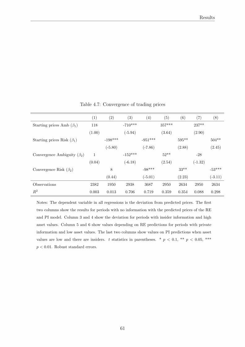
Results
Table 4.7: Convergence of trading prices
(1) (2) (3) (4) (5) (6) (7) (8)
Starting prices Amb (β1) 118 -710*** 357*** 237**
(1.00) (-5.94) (3.64) (2.90)
Starting prices Risk (β1) -198*** -951*** 595** 504**
(-5.80) (-7.86) (2.88) (2.45)
Convergence Ambiguity (β2) 1 -152*** 52** -28
(0.04) (-6.18) (2.54) (-1.32)
Convergence Risk (β2) 8 -98*** 33** -53***
(0.44) (-5.01) (2.23) (-3.11)
Observations 2382 1950 2938 3687 2950 2634 2950 2634
R2 0.003 0.013 0.706 0.719 0.359 0.354 0.088 0.298
Notes: The dependent variable in all regressions is the deviation from predicted prices. The first
two columns show the results for periods with no information with the predicted prices of the RE
and PI model. Column 3 and 4 show the deviation for periods with insider information and high
asset values. Column 5 and 6 show values depending on RE predictions for periods with private
information and low asset values. The last two columns show values on PI predictions when asset
values are low and there are insiders. t statistics in parentheses. * p < 0.1, ** p < 0.05, ***
p < 0.01. Robust standard errors.
61

Chapter 4: Ambiguity and Information Aggregation in Asset Markets
in periods with high asset fundamental value and slightly overpriced in periods with low
asset fundamental value and asset holdings do not reflect the predictions of the RE
model, we investigate the effect of ambiguity on the likelihood of trading around prices
predicted by the MM model versus prices predicted by the PI model. We employ the
subsample when there is private information in the market and the dividend is low as
both models predict different prices in the bad state with private information. To exploit
the likelihood of prices being at the MM levels we estimate the following equation using
a Logit regression:
Z = αi + β1Time+ β2DAmbiguity + β3Time ∗ Ambiguity + ε (4.2)
Z =
{1; if price closer to Maxmin level
0; if price closer to PI level in period without information
We introduce a dummy variable which takes the value one if a trading price
is closer to the maxmin level than to the PI level. The Time variable captures the
effect of time, which is in this setting close to trading activity, on the convergence of
prices. The dummy variable Ambiguity equals 1 if for observations in the market with
ambiguity and 0 otherwise. If discarding information overrules the pessimistic beliefs
under ambiguity, we expect that ambiguity will have a negative effect on the likelihood of
prices reaching the MM prices. Furthermore, we include an interaction term of ambiguity
and time to consider the effect of time under ambiguity since the pace of convergence
might be affected by the presence of ambiguity. The regression results are presented
in Table 4.8. The probability that prices at MM levels is positively affected by time,
which holds for all specifications. This finding is quite intuitive as some trading activity
should precede before private information will be disseminated in markets. For the
aggregate sample the effect of ambiguity in payoffs decreases the likelihood of information
dissemination in markets. This result also holds for the first treatment in which there is
ambiguity about the state probabilities. Including the interaction term shows that the
effect of time in the absorption of information is impeded by ambiguity. In treatment two
ambiguity has a positive effect on information absorption. This effect might be driven by
increased pessimistic beliefs as depicted by maxmin expected utility where prices equal
the maximum price of the minimum outcome between all traders.
Restricting the analysis to the subsample of private information with low dividend
discards trading in periods with high dividend. In these periods we expect that ambiguity
62

Results
Table 4.8: Convergence of prices to RE/Maxmin levels relative to PI prices
(1) (2) (3) (4) (5) (6)
Time 0.008*** 0.010*** 0.005*** 0.006*** 0.013*** 0.015***
(13.54) (11.00) (7.51) (5.41) (12.68) (10.40)
Ambiguity -0.221*** 0.076 -0.229*** -0.123 -0.088 0.329*
(-3.88) (0.66) (-3.25) (-0.86) (-0.87) (1.66)
Time*Ambiguity -0.003*** -0.001 -0.005**
(-2.92) (-0.84) (-2.40)
Constant -0.542*** -0.702*** -0.425*** -0.485*** -0.843*** -1.044***
(-8.55) (-8.41) (-5.37) (-4.57) (-7.82) (-7.63)
Observations 5197 5197 3406 3406 1791 1791
Notes: The dependent variable in all regressions is the dummy variable taking the value 1 if trading
price is closer to RE instead of PI level. Column 1-2 contain the aggregate data, in column 4-5
the sample is restricted to treatment 1. The last two columns contains the sample of treatment 2.
t statistics in parentheses. * p < 0.1, ** p < 0.05, *** p < 0.01. Robust standard errors.
has a more pronounced effect as the aversion to ambiguity leads to pessimistic belief
forming and discarding valuable information in asset prices which has more downward
potential in periods with high asset values. To test this we construct another dependent
variable which equals 1 if a price deviates at most 10 percent from the predicted level of
RE. With this specification we test whether ambiguity affects the likelihood of inferring
information from trading prices. Except for the difference in the construction of the
dependent variable we also include a dummy variable Dividend, which takes the value
1 if the dividend is high and 0 otherwise, to investigate the effect of high and low
dividend. In addition, we include an interaction term which captures a potential effect
of asymmetric reaction to news under ambiguity. The results, as demonstrated in Table
4.9, show that time has a similar positive effect on the convergence of prices towards the
RE prices. The divergence from predicted levels is higher in period with high dividend.
Ambiguity in markets decreases the likelihood of prices being at RE levels and this effect
is more pronounced in periods with high dividend.
Profits of informed vs uninformed traders
The models also predict a divergent outcome regarding the value of inside information.
According to RE model predictions, insider information should not contain an extra
63

Chapter 4: Ambiguity and Information Aggregation in Asset Markets
Tab
le4.9:
Con
vergence
ofprices
toR
E/M
axm
inlevels
(1)
(2)(3)
(4)(5)
(6)(7)
(8)(9)
Tim
e0.0
07***
0.006***0.006***
0.007***0.005***
0.005***0.009***
0.009***0.009***
(15.57)
(10.30)(10.08)
(11.48)(6.84)
(6.94)(10.75)
(8.20)(7.36)
Am
big
uity
-0.163**
*-0.335***-0.171
-0.238***-0.510***-0.147
-0.0620.022
-0.117
(-3.36)
(-3.18)(-1.48)
(-4.00)(-3.91)
(-1.03)(-0.72)
(0.12)(-0.56)
Tim
e*amb
0.002*0.002*
0.003**0.003**
-0.0010.000
(1.84)(1.79)
(2.36)(2.16)
(-0.51)(0.03)
Div
iden
d-0.410***
0.364***-1.949***
(-6.16)(4.36)
(-14.76)
Div
iden
d*a
mb
-0.542***-0.713***
0.119
(-5.37)(-5.73)
(0.62)
Con
stant
-2.072***-1.995***-1.752***-1.716***-1.594***-1.816***-2.685***-2.723***-1.779***
(-36.9
5)(-29.43)
(-22.66)(-24.90)
(-19.21)(-18.93)
(-27.23)(-21.80)
(-12.36)
Ob
servation
s115
27
1152711527
65446544
65444983
49834983
Notes:
The
dep
enden
tva
riable
inall
regressio
ns
isth
edu
mm
yva
riable
takin
gth
evalu
e1
ifth
ep
ricedoes
not
dev
iate
more
than
10
percen
tfro
mth
eR
Eprice.
Colu
mn
1-2
contain
the
aggregatedata,
incolu
mn
4-5
the
sam
ple
isrestricted
totrea
tmen
t1.
The
last
two
colu
mn
sco
ntain
sth
esam
ple
oftreatm
ent
2.t
statisticsin
paren
theses.
*p<
0.1
,**p<
0.0
5,
***p<
0.0
1.
Robu
ststan
dard
errors.
64

Results
Figure 4.1: Profits of subject with and without private information per state
dollar value as information is quickly spread in the market. Therefore, the trader with
inside information should not outperform other market participants. On the contrary,
the PI and maxmin model predict that insiders will outperform the rest of the market as
this information will be kept private. Figure 4.1 shows that informed traders on average
outperform uninformed traders in both markets. We observe that the gain from private
information is related to the state of the economy. The difference in profits between
informed and uninformed traders is larger in periods when the bad state occurs under
risky payoff fundamentals. This points again to more suppressed prices under ambiguity
which decreases potential profits from private information. In periods with a good state
we observe that inside information is more valuable in markets with ambiguity as the
downward deviation of prices creates more profit potential for insiders. In Figure 4.2 the
profits of informed and uninformed traders are demonstrated for the Treatment 2. The
graphs show that in the second treatment insiders are gain more profit from their private
information. This is particularly true for periods with high dividend (good state). The
graph shows that when the insider has positive information he makes larger profits when
the payoff level is ambiguous. This could be explained by the conservative bidding of
uninformed traders under ambiguity.
4.3.3. Prices and Information mirages
To test whether individuals falsely infer signal from prices and trade according to their
beliefs in a period with private information, we focus on the predictions of the RE model.
This model predicts that the expectations of an individual is endogenously determined
and hence might create this pattern. We find that in 10 percent of the periods with
65

Chapter 4: Ambiguity and Information Aggregation in Asset Markets
Figure 4.2: Profits of subject with and without private information per state - Treatment
2
no private information in the market an information mirage occurs. In periods with
no informed traders we find that subjects tend to follow expected payoff prices more
carefully when the underlying payoff distribution is uncertain rather than risky. Only 2
out of 16 periods are in markets with ambiguity. When payoff uncertainty increases due
to ambiguity, individuals might restrain themselves from inferring signals from submitted
prices as they put less value on other less precise sources of information and let themselves
be guided by the information they are provided with. Individuals might be less likely to
form beliefs based on potential signals as their initial knowledge and beliefs are shaped
with less certainty and thereby are not anchored deeply. Another explanation might be
that individuals tend to become less prone to biases, like overconfidence, when they are
provided with more uncertainty. A third channel through which the wrong inference of
positive information is suppressed in periods when there are no insiders in the market
might be ambiguity aversion. As individuals tend to show aversion to ambiguity, they
will be less likely to submit high prices and thereby prices will not be inflated and will
approach their expected values. We test the effect of ambiguity on the likelihood of the
occurrence of a mirage with the following specification:
Z = αi + β1,iDAmbiguity + ε (4.3)
Z =
{1; if mirage occurs
0; if no mirage
Ambiguity in the payoff of an asset decreases the likelihood of the occurrence of a
66

Conclusion
Table 4.10: Information mirages
mirage mirage mirage
Ambiguity -2.169*** -1.053*** -0.155***
(-2.79) (-3.08) (-3.30)
Constant -1.520*** -0.917*** 0.179***
(-5.13) (-5.51) (4.10)
Observations 160 160 160
R2 0.067
Notes: Column 1 shows the regression results of a Logit model, while column 2 demonstrates a Probit
regression. The last column shows OLS results. t statistics in parentheses. * p < 0.1, ** p < 0.05, ***
p < 0.01. Robust standard errors.
mirage. This effect is significant at a 1 percent level for different specifications. The
marginal effect of ambiguity on the formation of a mirage is -0.155. The presence of
ambiguity might increase the effect of holding on to one’s prior beliefs. Mirages are 4
times more likely under ambiguity about the payoff range than about the probability
range.
4.4. Conclusion
Previous research has documented that ambiguity impedes the information aggrega-
tion function of prices and the RE equilibrium is partially revealing. In an experimental
double auction asset market we investigated the effect of ambiguous beliefs about fun-
damentals of an asset on private information dissemination. We isolated the effect of
ambiguity by creating two identical asset markets which enabled us to impose differ-
ent levels of uncertainty while investigating the dissemination of private information. In
periods with insiders, prices do not converge to RE levels in risky nor ambiguous markets.
However, we find that ambiguity strengthens the deviation of trading prices from
the fundamental value even more and thereby hampers the absorption of information
more severely. This negative effect on the probability of a convergence towards RE prices
is particularly true for periods when the value of the traded asset is high. Good news
67

Chapter 4: Ambiguity and Information Aggregation in Asset Markets
is perceived with more caution and under-weighted by uninformed traders which keeps
prices suppressed and lower than fundamentals, while this result holds for both risky and
ambiguous markets, it is stronger when ambiguity is present. This finding is coherent
with previous findings on ambiguity and information aggregation in asset markets as the
reaction to negative news by investors is stronger as bad news is over- weighted (Epstein
and Schneider (2008)). Ambiguity also decreases the pace of information transmission in
asset markets. The convergence towards fundamental values is at a slower level, insiders
are given more potential to outperform other traders in the market. We should notice
that more data is needed in order to rule out any order effects which might be present
with the current experimental design.
Furthermore, we find that in markets with risky payoffs information mirages occur
in periods when no private information is given, whereas individuals are more reluctant
to infer private information from observed trading prices when facing ambiguity. This
drives prices more to their expected values and eliminates information mirages to a large
extent.
4.5. Appendix
68

Appendix
4.5.1. Instructions
Dividend Payment In each period, the computer will randomly draw a value to determine
the dividend payment of the asset. In each period the dividend of the asset can take a
high value of 350 or a low value of 100 francs, depending on the random draw. These
high and low dividend might differ per trader. In the first 15 periods, the probability
with which the asset will pay a high dividend is an unknown percentage. The probability
that the asset will pay high dividend lies between 0% and 100%. But we do not know
the exact probability. It might be that the probability is 1% or 2% or 85% up till 100%.
In the last 15 periods, the probability that the asset will pay high dividend is 50%. .
Dividends Account The realized dividend in each period will be paid to you in a separate
account and it counts towards your final earnings. That is to say you cannot use your
dividends earnings to purchase assets. Furthermore, the dividend draws in each period
are independent, meaning that the likelihood of a particular dividend in a period is not
affected by the dividend in previous periods.
Each period, there is a 50% chance that the computer will provide the realized div-
idend to half of the randomly selected traders in this room. The selection is made
independently in each period, so that the chance that you would be selected to know
the dividend in a period is NOT affected by whether you were selected in any previous
period. You will get to know whether half of the traders knew the realized dividend or
not at the end of each period.
Your Earnings At the beginning of the experiment, you will be given 5000 francs in
cash together with 5 units of the asset in your inventory. Your profits for the entire
experiment come from two sources—from all the dividends you receive in your dividend
account and from buying and selling assets. All money spent on purchases is subtracted
from your cash account. All money received from sales is added to your cash account.
Thus, you can gain or lose money on the purchase and resale of assets. Your profit per
period equals the amount of francs in your cash account at the end of the period, plus
all dividends you earned that period.
Trading In each period, you will see a computer screen like the one shown below.
Each period will have a duration of 180 seconds. You are free to buy and sell assets
during the trading period.
69

Chapter 4: Ambiguity and Information Aggregation in Asset Markets
For purchasing the asset you can click on the offer which appears on your screen as
a sell offer and click afterwards on the button BUY. For selling the asset you own you
have to select a buy offer and afterwards click on the SELL button. The prices which
appear on the screen are per-unit prices. The market price in the middle of the screen
shows the last price at which the good has been traded in the market. At the end of each
period you will be shown an earnings screen on which the realized dividend is shown
along with your profits and the presence/absence of traders with information about the
realized dividend during the last trading period.
70

Appendix
71

Chapter 4: Ambiguity and Information Aggregation in Asset Markets
Tab
le4.11:
MSE
ofprices
frompred
ictedprices
by
RE
,M
axm
inan
dP
Im
odel
inth
elast
90secon
ds
Am
bigu
itym
arket
Risk
market
No
inform
ation
Bad
state
No
info
rmation
Bad
state
Sessio
nR
E/P
IM
axm
inG
ood
state
RE
/M
axm
inP
IR
E/P
IM
axm
inG
ood
state
RE
/Max
min
PI
154,18
58,0
191,4
744,1
948,6
941,0
2110,92
141,4848,05
42,02
281,97
134,1
353,5
779,9
876,0
2102,5
266,34
86,98138,04
97,89
356,29
31,6
168,6
441,0
938,4
539,6
838,13
131,0335,58
36,17
491,35
173,8
859,3
6153,4
386,9
4118,3
1177,75
57,85159,80
114,30
546,89
53,5
977,4
858,4
840,7
631,9
362,55
131,3282,30
46,07
655,41
47,1
280,0
941,6
735,2
436,8
193,76
145,3233,30
37,17
780,06
79,6
8106
,5567,1
756,0
276,5
052,79
174,9180,07
72,72
863,71
137,7
6234
,7672,3
988,4
161,0
9134,23
149,46127,70
41,41
950,09
73,1
5161
,8141,6
791,9
077,0
369,58
131,5036,17
99,49
10
60,1
2112
,1713
8,41
58,9
4108,2
6103,9
2160,87
97,3736,10
79,15
11
51,5
6111
,2522
2,50
23,5
469,1
199,7
4174,66
125,12658,10
72,44
12
123,7
1160
,8321
3,14
192,5
9149,2
995,7
1123,35
144,9768,67
141,02
72

Chapter 5
Time Discounting under Ambiguity
5.1. Introduction
Discount rates allow individuals to compare outcomes occurring at different times. Many
models of economic decision making include intertemporal utility functions. Predictions
of intertemporal choice models are greatly subject to discount rate sensitivity. There-
fore, the correct estimation of individual discount rates is crucial for economic modeling.
Observed individual discount rates in experimental studies range from 1 percent (Thaler,
1981)to well over 1000 percent Holcomb and Nelson (1992), which is substantially higher
than interest rates observed in markets. An extensive empirical and experimental litera-
ture has documented various anomalies in discounting behavior which questioned axioms
in economic modeling of preferences. Motivated by these findings a line of research in-
vestigated the relationship and interaction of time and risk preferences.
In this paper we examine the role of ambiguity on individual time preferences.
To our knowledge, there is no theoretical nor experimental study which shows predic-
tions or experimental evidence on individual discounting behavior under ambiguity. In
a laboratory experiment we assessed individual discount rates in the presence of risky or
ambiguous prospects in order to identify differences in time preferences under different
levels of uncertainty. Where the former describes an uncertain payment when probabil-
ities about future outcomes are known, the latter concerns an uncertain payment when
probabilities about future outcomes are not (fully) known. We investigate differences
in individual discount rates inferred from risky and ambiguous decisions for a range of
horizons. With our experimental design we can identify differences in discount rates by
varying the uncertainty levels of payout probabilities, with other inputs held constant.
Our results show that discount rates differ from discounting under risk when subjects
have an imprecise knowledge of the payoff probabilities. This points to differences in dis-
count rates driven by ambiguity and should be considered when modeling or estimating
73
Chapter 5: Time Discounting under Ambiguity
dynamic choices in economics.
A strand of literature studied the interaction of time and risk preferences as these
cannot be considered as orthogonal dimensions of decision making under uncertainty.
Some studies found correlation between risk and time preferences by linking risk aver-
sion levels with discount rates of individuals. These studies show that risk aversion
levels are positively correlated with discounting behavior of subjects ((Anderhub et al.,
2001), (Andersen et al., 2008)). The framework of various dynamic choice models have
incorporated risk preferences in explaining time preferences and estimating individual
and social discount rates ((Kreps and Porteus, 1978), Epstein and Zin (1989)). (Epper
et al., 2011) attempt to unify risk and time preferences and show that probability weight-
ing is a common factor in shaping risk and discounting behavior. Experimental studies
investigated people’s choices in the presence of risk and delay ((Keren and Roelofsma,
1995),(Weber and Chapman, 2005), (Noussair and Wu, 2006), (Anderson and Stafford,
2009), (Baucells and Heukamp, 2010)). These studies generally conclude that there are
interaction effects between time and risk, such as risk tolerance increasing with delay.
However, preferences towards risk should be distinguished from preferences towards
ambiguity ((Knight, 2012) and (Ellsberg, 1961)). Therefore, time preferences should be
disentangled from both preferences towards risk and ambiguity. Recent models have
extended the notion of uncertainty and have replaced the unique probability function
shaping the decision maker’s beliefs by a set of probability functions. (Gierlinger et al.,
2008) and (Traeger, 2014) show that the social discount rate is lower under ambiguity.
In an experimental setting we test for the effect of ambiguity on the discount rates of
individuals and find evidence that ambiguity plays a significant role in intertemporal
decision making. While ambiguity typically induces pessimistic beliefs and thereby de-
creases the expected value of a decision task under risk, we find that individuals use
lower or higher individual discount rates when prospects which will be paid out in the
future are ambiguous rather than only risky, depending on how ambiguity is presented
to subjects. A study by (Weber and Tan, 2012) shows that ambiguity aversion is also
present for delayed options. Our study complements this finding by demonstrating that
discount rates are affected by the presence of ambiguity.
Our study also contributes to a line of research showing the sensitivity of time
preferences to different parameters of the decision task. Some anomalies which are doc-
74

Experiment
umented in time discounting are process dependence, diminishing impatience ((Laibson,
1997)), the common difference effect ((Bleichrodt and Johannesson, 2001)), the com-
mon ration effect ((Kahneman and Tversky, 1979)) and the magnitude effect (Thaler,
1981)(Sun and Potters, 2016) (Halevy, 2015). Other studies have shown that discount
rates tend to be higher for certain future payoffs than discount rates for risky future
payoffs. People’s preference for present certain outcomes over delayed ones, immediacy,
weakens drastically when the outcomes become risky ((Keren and Roelofsma, 1995),(We-
ber and Chapman, 2005)). Our study relates to this literature as we introduce another
dimension of uncertainty. We find a magnitude effect for risky and ambiguous prospects
and thereby show that the magnitude effect is also present when payoffs contain ambi-
guity depending on how ambiguity is presented to subjects.
The rest of the paper is organized as follows. Section 5.2 describes the experimental
design and procedures. Section 5.3 summarizes the data and estimations of individual
discount rates. Section 5.4 concludes.
5.2. Experiment
5.2.1. Design
To elicit individual discount rates under risk or ambiguity, individuals had to reveal
their preference between two prospects. In each period, subjects are presented with
eight pairs of binary prospects (p, xt)T=2 and (p, (x + b)t)T=z, where Z=4,..,8 describes
the payout date in weeks, t=1,..,80 represents the period in the experiment and b =
0.025∗xt, ..., 0.2∗xt, corresponds to the extra amount which is offered with the prospect
which has a later payout date. The extra amount offered for the payment which lies
further in the future increases in percentages of 2.5 percent of xt. Each pair of prospects
results in outcome x (or x+b) with probability p and in outcome 0 with probability 1-p.
Subjects were asked to make a choice between the eight paired prospects displayed on
each screen. If the subject prefers to play the lottery (p, xt)T=2 in two weeks, we can
infer that the person has a higher discount rate than the interest rate which is offered
with the paired lottery (p, (x + b)t)T=z. By increasing b we find the amount for which
the individual switches from the early prospect to the prospect with the later payout
75

Chapter 5: Time Discounting under Ambiguity
date. We can then infer that the discount rate of the subject lies around this point.
The parameters p, xt, Z and T were fixed in each period t, while the extra amount b
was varying per pair of prospect. At the end of the experiment, the computer randomly
selected one period and one of the decisions of that period to determine the subject’s
earnings. Depending on the choice of the subject, the subject was paid out the outcome
of the lottery at the date attached to that lottery.
In designing ambiguous lottery payments we have used to approach used by i.a.
(Maafi, 2011) and citehuber2014experimental by implementing ambiguity by providing
ranges for the probabilities of outcomes. Each session consisted of 80 periods and four
different sections which differed in how p was determined, which reflected the nature
of uncertainty. Per section of 20 periods the prospects contained either 1) only risk,
where the probability of a positive payout p is known to the subject and fixed within
these 20 periods 2) high ambiguity, where the probability of a positive payout p was
given as a range between 0 and 100 which describes a probability of a positive payoff
drawn from a probability distribution between 0 and 100. 3) lower levels of ambiguity,
where the probability of a positive payoff was drawn from smaller distribution intervals.
4) Unknown levels of p where subjects were not provided with any information about
the probability of the positive payout and p was missing. In this section subjects were
informed that with some probability they would receive xt in two weeks or (x+ b)t)T=z
in z weeks time depending on their choice.
The parameters used in the experiment are summarized in Table 5.1. Each row
indicates the range of values in the respective periods of the experiment. With this de-
sign we elicited discount rates for five different time horizons and four different amount
of monetary stakes under 4 different uncertainty levels. Instead of extrapolating one dis-
count rate to multiple horizons, we directly elicited discount rates for different horizons.
The payout horizon of the early prospect was in all periods equal to two weeks, while
the payout date of the prospects with the higher payment varied between four and eight
weeks. By having both payouts in the future, we isolate time preferences which is only
driven by the level of impatience. The choices in periods were similar and differed only
in either 1) the monetary stakes xt varying between 1000 and 4000 Experimental Francs
and (x+b)t)T=z varying between 1025 and 4800 Experimental Francs, 2) the payout date
of the later prospect to obtain discount rates for horizons of 2,3,4,5 and 6 weeks., or 3)
76

Experiment
the formulation of p with which different uncertainty levels were imposed. If subjects
assume that all probabilities in between the given intervals are equally likely, they can
calculate a probability value equal to .5. These parameters were used throughout the
experiment and were repeated for each ”type” of uncertainty.
The main advantage of using a multiple price list (MPL) format to elicit time
preferences is that it is relatively transparent to subjects and provides simple incentives
for truthful revelation. On the other hand, the main disadvantage is potential suscepti-
bility to framing effects as revealed preferences might be sensitive to procedures, subject
pools, and the format of the multiple price list table. In addition, using an MPL for-
mat to elicit discount rates appear less sensitive to details of the experimental design.
A recent theoretical study by (Bade, 2015) suggests that there exists a problem with
using the random lottery incentive system in ambiguity experiments, since it provides
opportunities for subjects to hedge. The paper discusses preference reversals with ran-
domized experiments in the presence of risk and ambiguity. It also allows for different
utility derived from risk and ambiguity. In this experiment ambiguous payoffs are not
assumed to provide different utility and in addition we investigate the time preference of
individuals in isolation of either risk or ambiguous lotteries.
An example of the task in period subjects were facing is demonstrated in Table
5.2. In this period in the experiment the subject faced 8 choices between preferring to
receive xt or ((x + b)t)T=8. The early prospect was identical for all eight choices. In
this particular period the prospect which was paid out at the early date would pay out
2000 Experimental Francs with p probability, where p=[0,100]. This prospect xt was
paired with a prospect with payout date 8 weeks after the experiment, where the extra
amount b was increasing per choice. The probability with which the later prospect paid
out ((x+ b)t) was similar for both prospects. Subjects faced ambiguous payoffs for each
alternative. For illustration purposes we included the annual interest rate belonging to
each alternative. However this information was not present in the experiment.
5.2.2. Procedures
The experiment was conducted at the Centerlab of Tilburg University in The Nether-
lands. A total of 70 Economics and Business Administration students participated in 7
sessions. The sessions were conducted between March 2015 and May 2015. The experi-
77

Chapter 5: Time Discounting under Ambiguity
Table 5.1: Parameters used in the experiment
t T xt (x+ b)t p
1 - 5 2 - 6 2000 2050 - 2400 10% - 90%
6 - 10 2 - 6 2000 2050 - 2400 20% - 80%
11 - 15 2 - 6 2000 2050 - 2400 30% - 70%
16 - 20 2 - 6 2000 2050 - 2400 40% - 60%
21-25 2 - 6 1000 1025 - 1200 0% - 100%
26-30 2 - 6 2000 2050 - 2400 0% - 100%
31-35 2 - 6 3000 3075 - 3600 0% - 100%
36-40 2 - 6 4000 4100 - 4800 0% - 100%
41-45 2 - 6 1000 1025 - 1200 50%
46-50 2 - 6 2000 2050 - 2400 50%
51-55 2 - 6 3000 3075 - 3600 50%
56-60 2 - 6 4000 4100 - 4800 50%
60-65 2 - 6 1000 1025 - 1200 Unknown
66-70 2 - 6 2000 2050 - 2400 Unknown
71-75 2 - 6 3000 3075 - 3600 Unknown
76-80 2 - 6 4000 4100 - 4800 Unknown
Table 5.2: Example of the choices subjects had to make each period
Choice xt ((x+ b)t)T=8 p Annual Interest rate
(payout in 2 weeks) (payout in 8 weeks)
1 2000 2050 [0,100] 16.25%
2 2000 2100 [0,100] 32.5%
3 2000 2150 [0,100] 48.75%
4 2000 2200 [0,100] 65%
5 2000 2250 [0,100] 81.25%
6 2000 2300 [0,100] 97.5%
7 2000 2350 [0,100] 113.75%
8 2000 2400 [0,100] 130%
The gender variable contains 5 missing values.
78

Results
ment was executed with the z-Tree computer program (Fischbacher (2007)). There were
a varying number of participants per session and each subject acted independently in this
individual decision making experiment. Each session lasted approximately 45 minutes.
The payoffs in the experiment were calculated in terms of experimental currency, which
was converted to Euros at the end of the session. The average earnings per subject were
28 Euros. The exchange rate used in the experiment was 100 Experimental Francs to
1 Euro. In order to eliminate a potential present-bias effect by subjects to receive the
earnings at the end of the experiment, the earliest payout date was set at 2 weeks from
the date of participation. Subjects were paid by bank transfer on the date which was
determined by their choices in the experiment.
5.3. Results
Data on the time preferences of 57 subjects were used for the analysis as the rest
of our subject pool demonstrated repeated inconsistent responses. If a subject provided
inconsistent preferences more than 5 times during the experiment, he/she was eliminated
from the subject pool for the analysis, otherwise only the inconsistent choice was deleted.
Given that there is no theory which models individual discount rates under ambiguity,
we expect that elicited discount rates would be similar under risk as under ambiguity.
The average annual discount rates which are inferred from the choices of subjects are
reported in Table 5.3. The numbers demonstrate that individuals discount future payoffs
at a lower level when payoffs are ambiguous rather than risky when ambiguous prospects
are presented with a probability distribution. These differences average discount rates
are in almost half of the cases also statistically significant. While this effect is true for
different payoff levels, the difference in impatience decreases as payoffs increase. The
difference in discount rates is also in non of the cases significant when stakes get large.
When the late prospects is paid out in the more distant future we observe that the
difference between discounting risky and ambiguous payoffs becomes less pronounced.
Furthermore, these numbers point out that inferred annual interest rates show sensitivity
to the horizon which is used to elicit discount rates. In line with studies showing a
magnitude effect in discounting, we also find that higher payoff levels are less heavily
79

Chapter 5: Time Discounting under Ambiguity
discounted. Individuals show more patience when stakes are higher. When payoffs are
ambiguous and there is no information about probabilities given to subjects, discount
rates are lower and statistically significant when the payout horizon increases.
Figure 5.1 displays the distribution of individual discount rates per payoff level.
The discount rate of each individual is calculated as the average discount rate for each
payoff level inferred from choices with different payment horizons. The figure shows
that a sizeable share of individuals use higher discount rates when facing a risky payoff
decision. However, this difference vanishes when stakes get higher. With a Kolmogorov-
Smirnov test we conclude that we cannot reject the hypothesis of the equality of both
distributions with p=.29 for the aggregate data. The analysis in the paper implicitly
assumes that subjects are risk neutral. However, if we allow for concavity of the utility
curve of an individual, then receiving a higher amount in the future should first be
corrected with the risk aversion level of the individual If we do not correct for this, we
might wrongly elicit discount rates which are higher than the true discount rate of the
subject. The stakes in my experiment are small enough to assume they are risk neutral.
In order to verify the effect of ambiguity on the discounting behavior of individuals
we estimate specification 5.1. We regress discount rates as a function of ambiguity. We
also control for the payoff level, xt and the horizon in weeks which is used to elicit the
yearly discount rate. Da corresponds to the dummy variable taking the value 1 if the
payoff is ambiguous, and 0 otherwise. ε is distributed iid. Table 5.3 and 5.5 demonstrate
the results of this specification along with regression results of this specification when
interaction effects are included as ambiguity might also effect discount rates through
a potential magnitude effect or might change the effect which varying horizons have on
time preferences. For these estimations we use the subsample of choices in which subjects
either face risky prospects with p=0.5 or high ambiguous prospects with p=[0,100] or
ambiguous prospects without any probability distribution separately. The results in
Table 5.3 show that prospects with ambiguous payoffs are discounted at a lower rate
when a range of probabilities is provided. On the contrary, Table 5.5 demonstrates
that discounting under ambiguity without any probability range is higher. While higher
stakes xt are discounted at a lower rate, we find that ambiguity only has an effect on this
when there subjects are not given a probability distribution. We also observe that the
horizon which is used to elicit discount rates seem to be important for the impatience
80

Results
Table 5.3: Elicited Average Yearly Discount Rates
xt T = 4 T = 5 T = 6 T = 7 T = 8
Ambiguity p=[0,100] 1000 227% 161% 146% 124% * 113% *
Risk 1000 247% 189% 158% 133% 126%
Ambiguity p=unknown 1000 147% 124% 147% * 145% 133%
Ambiguity p=[0,100] 2000 194% * 135% * 126% 111% 104 %
Risk 2000 224% 157% 127% 112% 107%
Ambiguity p=unknown 1000 161% 123% 142% * 126% * 120% *
Ambiguity p=[0,100] 3000 152% * 110% * 102% * 94% * 91% *
Risk 3000 171% 133% 118% 105% 98%
Ambiguity p=unknown 1000 149% 112% 125% * 109% 105% *
Ambiguity p=[0,100] 4000 134% 110% 102% 98% 90%
Risk 4000 137% 115% 105% 95% 92%
Ambiguity p=unknown 1000 122% 99% * 106% 103% 0.95%
Each column corresponds to discount rates elicited from choices with horizon T.
* The difference in means between discounting under risk and discounting under
ambiguity is statistically significant at 10% significance level.
81
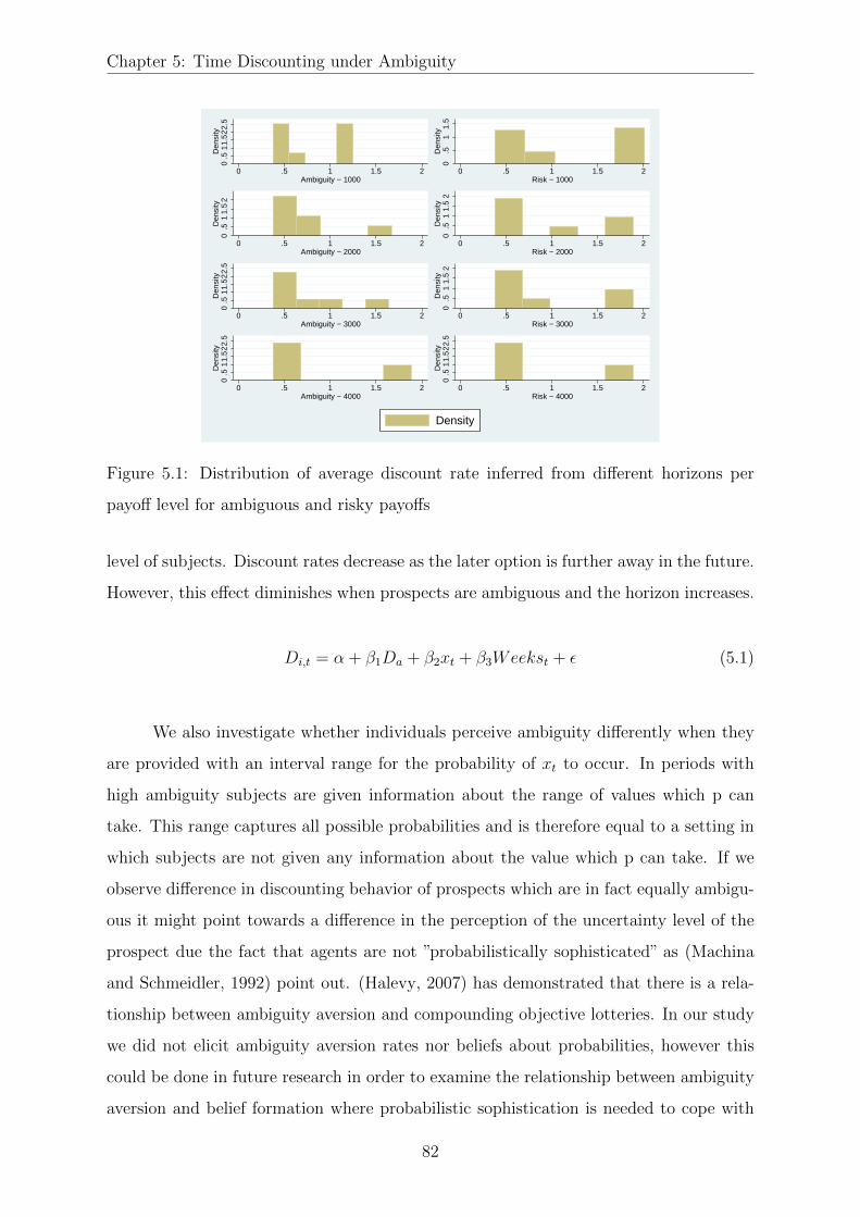
Chapter 5: Time Discounting under Ambiguity
0.5
11.
52
2.5
Den
sity
0 .5 1 1.5 2Ambiguity − 1000
0.5
11.
5D
ensi
ty
0 .5 1 1.5 2Risk − 1000
0.5
11.
52
Den
sity
0 .5 1 1.5 2Ambiguity − 2000
0.5
11.
52
Den
sity
0 .5 1 1.5 2Risk − 2000
0.5
11.
52
2.5
Den
sity
0 .5 1 1.5 2Ambiguity − 3000
0.5
11.
52
Den
sity
0 .5 1 1.5 2Risk − 3000
0.5
11.
52
2.5
Den
sity
0 .5 1 1.5 2Ambiguity − 4000
0.5
11.
52
2.5
Den
sity
0 .5 1 1.5 2Risk − 4000
Density
Figure 5.1: Distribution of average discount rate inferred from different horizons per
payoff level for ambiguous and risky payoffs
level of subjects. Discount rates decrease as the later option is further away in the future.
However, this effect diminishes when prospects are ambiguous and the horizon increases.
Di,t = α + β1Da + β2xt + β3Weekst + ε (5.1)
We also investigate whether individuals perceive ambiguity differently when they
are provided with an interval range for the probability of xt to occur. In periods with
high ambiguity subjects are given information about the range of values which p can
take. This range captures all possible probabilities and is therefore equal to a setting in
which subjects are not given any information about the value which p can take. If we
observe difference in discounting behavior of prospects which are in fact equally ambigu-
ous it might point towards a difference in the perception of the uncertainty level of the
prospect due the fact that agents are not ”probabilistically sophisticated” as (Machina
and Schmeidler, 1992) point out. (Halevy, 2007) has demonstrated that there is a rela-
tionship between ambiguity aversion and compounding objective lotteries. In our study
we did not elicit ambiguity aversion rates nor beliefs about probabilities, however this
could be done in future research in order to examine the relationship between ambiguity
aversion and belief formation where probabilistic sophistication is needed to cope with
82

Results
Table 5.4: Discount rates where ambiguity corresponds
to prospects with p=[0,100]
(1) (2) (3)
Dambiguity -0.117** -0.236* -0.479**
(-2.43) (-1.92) (-2.09)
xt -0.000*** -0.000*** -0.000***
(-5.85) (-5.85) (-5.85)
Weeks -0.208*** -0.208*** -0.218***
(-5.94) (-5.94) (-6.20)
Ambiguity*xt 0.000 0.000
(1.42) (1.42)
Ambiguity*Weeks 0.040**
(2.01)
Constant 3.129*** 3.165*** 3.226***
(8.20) (8.27) (8.34)
Observations 4549 4549 4549
R2
t statistics in parentheses. * p < 0.1, ** p < 0.05,
*** p < 0.01. Robust standard errors clustered at
subject level.
83

Chapter 5: Time Discounting under Ambiguity
Table 5.5: Discount rates where ambiguity is defined
without any probability distribution
(1) (2) (3)
Dambiguity 0.222*** 0.467*** 0.883***
(3.14) (3.40) (3.47)
xt -0.000*** -0.000*** -0.000***
(-6.00) (-5.71) (-5.71)
Weeks -0.208*** -0.208*** -0.190***
(-5.94) (-5.94) (-5.36)
Ambiguity*xt -0.000*** -0.000***
(-2.91) (-2.91)
Ambiguity*Weeks -0.069***
(-3.28)
Constant 3.070*** 2.995*** 2.892***
(8.11) (7.96) (7.71)
Observations 4549 4549 4549
R2 0.065 0.066 0.067
t statistics in parentheses. * p < 0.1, ** p < 0.05,
*** p < 0.01. Robust standard errors clustered at
subject level.
84

Results
0.5
11.
52
2.5
Den
sity
0 .5 1 1.5 2p=[0,100] − 1000
0.5
11.
5D
ensi
ty
0 .5 1 1.5 2p=unknown − 1000
0.5
11.
52
Den
sity
0 .5 1 1.5 2p=[0,100] − 2000
0.5
11.
5D
ensi
ty
0 .5 1 1.5 2p=unknown − 2000
0.5
11.
52
2.5
Den
sity
0 .5 1 1.5 2p=[0,100] − 3000
0.5
11.
5D
ensi
ty
0 .5 1 1.5 2p=unknown − 3000
0.5
11.
52
2.5
Den
sity
0 .5 1 1.5 2p=[0,100] − 4000
0.5
11.
52
Den
sity
0 .5 1 1.5 2p=unknown − 4000
Density
Figure 5.2: Distribution of average discount rate inferred from different horizons per
payoff level for prospects with an interval of probabilities provided to subjects versus
prospects without any information about payout probabilities
the descriptive problem. While (Krain et al., 2006) measure activation of orbitofrontal
and lateral frontal cortices and show that decision making under ambiguity induce more
cognitive load decision making under risk as the DLPFC activity is more intense with
tasks involving ambiguity, another finding by (Benjamin et al., 2013) shows that the rela-
tionship between cognitive ability and time preferences is specific to intertemporal pref-
erences when individuals reveal preferences between immediate and delayed payments.
This relationship fades away when time preferences are measured between different de-
layed rewards, which is used in our experiment. Figure 5.2 demonstrates the distribution
of individual interest rates for both settings. It is apparent that subjects use lower in-
terest rates to discount prospects when the probability range for p is explicitly given.
This points towards perceiving an ambiguous prospect without probabilities differently.
With a Kolmogorov-Smirnov test we conclude that we can reject the hypothesis of the
equality of both distributions with p=.000.
(Curley and Yates, 1985) and (Larson, 1980) have demonstrated that ambiguity
avoidance increased with the range of probabilities. We asses whether the aversion to
increasing ranges of probabilities has an effect on discounting behavior by investigating
time preferences derived from prospects with different ambiguity levels and allowing
85

Chapter 5: Time Discounting under Ambiguity
for different coefficient estimates for varying ambiguity levels. We use a cross section
of our data and include data on time preferences of individuals for a payoff level of
2000 Experimental Francs. For this cross section we have data on discount rates where
the level of ambiguity of the payout probabilities stepwise vary. We use the degree of
ambiguity as a categorical variable in explaining discount rates. The specification we
run is the following:
Di,t = αi + β1Da + β2Weekst + ε (5.2)
where
Da =
0; p=[0.5]
1; p=[0.4,0.6]
2; p=[0.3,0.7]
3; p=[0.2,0.8]
4; p=[0.1,0.9]
5; p=[0,1]
The results in Table 5.6 show that discount rates are only affected by ambiguity
when the ambiguity level is highest. Subjects discount prospects with p=[0,1] at a lower
rate. For these prospects our dummy variable is almost significant at the 10 percent level.
This finding suggests that ambiguity does not have a linear effect on time preferences.
5.4. Conclusion
We investigated individual discount rates in the presence of ambiguous payoff prob-
abilities. In a laboratory experiment we elicited discount rates for risky and ambiguous
prospects separately. Our findings show that individuals use a lower discount rate when
they face ambiguity in the payout probabilities of prospects and a probability distri-
bution is provided. This effect changes sign when subjects are not provided with any
information regarding the payout probabilities and subjects discount at higher rates.
The difference in discounting behavior decreases as stakes get larger. Given that numer-
ous inter-temporal decision making tasks in economics contain ambiguity, this finding
shows that discounting under ambiguity differs from discounting under risk. This find-
86

Conclusion
Table 5.6: Discount rats
(1)
Weeks -1.688
(-1.61)
Da=0 0.000
(.)
Da=1 -0.077
(-1.18)
Da=2 -0.100
(-1.49)
Da=3 4.347
(0.97)
Da=4 4.343
(0.98)
Da=5 -0.114
(-1.62)
Constant 11.587∗
(1.83)
Observations 1710
R2 0.005
t statistics in paren-
theses. * p < 0.1, **
p < 0.05, *** p <
0.01. Robust stan-
dard errors clustered
at subject level.
87

Chapter 5: Time Discounting under Ambiguity
ing shows that next to the vast literature investigating the correlates and interaction of
risk and time preferences, the co-movements of time and ambiguity preferences might be
investigated.
Our findings also show that ambiguity in the probabilities of a positive payoff are
perceived differently when this feature is made salient as we find significant differences in
discounting between cases when probabilities are given as a range between 0 and 100 and
when no probability distribution is provided to subjects. This shows that the perception
of ambiguity and thereby discounting is highly subject to the information framing and
thereby might also affect time preferences.
Our results also have important implications for the current debate of informing
retail investors about the risk of financial holdings in asset markets. (Kaufmann et al.,
2013) shows evidence that the risk perception of financial products by investors is af-
fected by different risk presentation modes. Our findings supports this and shows that
individuals tend to perceive ambiguity differently depending on framing. If we would like
to induce more patience and long term orientation on retail investors’ financial decision
making, then providing information about probabilities might hurt. Not providing any
information about the probability distribution also decreases discount rates relative to
discount rates under risky decisions. In order to control for order effects, learning effects
and belief formation follow-up work should correct for belief formation under ambiguity
and also very the order of the risky and ambiguous lotteries. This would provide a more
comprehensive analysis of the effect of ambiguity on time preferences.
5.5. Appendix
88
Appendix
5.5.1. Instructions
The Experiment
This experiment is about decision making. The experiment consists of 80 periods.
Each period you will be presented a sequence of choices. The currency used in the
experiment is francs. The amounts which are presented to you are all in terms of francs.
You will be paid in cash in Euro’s according to your realized earnings by bank transfer.
The conversion rate is 100 francs to 1 Euro. In each period you will see a computer
screen like the one shown below:
Each presented choice consists of two options. Both options are lotteries with two
possible outcomes. A positive outcome with the probability(ies) given or 0 otherwise.
The probability with which the lottery will pay out the positive outcome is stated on
the screen. In each period you have to indicate for each choice which lottery you prefer.
Please notice that the pay-out date of the paired lotteries are different! The probability
with which the lottery pays out a positive amount is either 1) a known percentage 2) an
unknown percentage or 3) an interval of percentages. For example, looking at Example
1 we see that Lottery 1 pays out 1000 Francs. The probability that it will pay out lies
between 10% and 50%. It might be that the probability is 11% or 12% or 13% up till
50%. At the end of the experiment, the computer will randomly select one period and
one choice of that period to determine your earnings of this experiment. Each period has
equal probability to be selected by the computer and each choice has equal probability
to be selected by the computer.
Your earnings
You will start with an initial earning of 500 francs. After you have finished the
experiment by indicating your choices, the outcome of the round which will be played
for real will be added to your initial earnings and this will become your final earning of
the experiment.
89

Chapter 5: Time Discounting under Ambiguity
Figure 5.3: Example 1
Figure 5.4: Example 2
90

Bibliography
Abel, A. B. (1990). Asset prices under habit formation and catching up with the joneses.
The American Economic Review , 38–42.
Abeler, J., A. Falk, L. Goette, and D. Huffman (2011). Reference points and effort
provision. The American Economic Review , 470–492.
Ahn, D., S. Choi, D. Gale, and S. Kariv (2014). Estimating ambiguity aversion in a
portfolio choice experiment. Quantitative Economics 5 (2), 195–223.
Ameriks, J., A. Caplin, J. Leahy, and T. Tyler (2007). Measuring self-control problems.
The American Economic Review 97 (3), 966–972.
Anderhub, V., W. Guth, U. Gneezy, and D. Sonsino (2001). On the interaction of risk and
time preferences: An experimental study. German Economic Review 2 (3), 239–253.
Andersen, S., G. W. Harrison, M. I. Lau, and E. E. Rutstrom (2006). Elicitation using
multiple price list formats. Experimental Economics 9 (4), 383–405.
Andersen, S., G. W. Harrison, M. I. Lau, and E. E. Rutstrom (2008). Eliciting risk and
time preferences. Econometrica 76 (3), 583–618.
Anderson, L. R. and S. L. Stafford (2009). Individual decision-making experiments with
risk and intertemporal choice. Journal of Risk and Uncertainty 38 (1), 51–72.
Arkes, H. R., D. Hirshleifer, D. Jiang, and S. Lim (2008). Reference point adaptation:
Tests in the domain of security trading. Organizational Behavior and Human Decision
Processes 105 (1), 67–81.
Bade, S. (2015). Randomization devices and the elicitation of ambiguity-averse prefer-
ences. Journal of Economic Theory 159, 221–235.
91

Chapter 5: BIBLIOGRAPHY
Baillon, A., H. Bleichrodt, and V. Spinu (2015). Searching for the reference point.
Technical report, Working Paper.
Barberis, N., A. Shleifer, and R. Vishny (1998). A model of investor sentiment. Journal
of financial economics 49 (3), 307–343.
Barseghyan, L., J. Prince, and J. C. Teitelbaum (2011). Are risk preferences stable
across contexts? evidence from insurance data. American Economic Review 101 (2),
591–631.
Baucells, M. and F. H. Heukamp (2010). Common ratio using delay. Theory and Deci-
sion 68 (1-2), 149–158.
Baucells, M., M. Weber, and F. Welfens (2011). Reference-point formation and updating.
Management Science 57 (3), 506–519.
Bell, D. E. (1985). Disappointment in decision making under uncertainty. Operations
Research 33 (1), 1–27.
Benjamin, D. J., S. A. Brown, and J. M. Shapiro (2013). Who is ‘behavioral’? cogni-
tive ability and anomalous preferences. Journal of the European Economic Associa-
tion 11 (6), 1231–1255.
Bleichrodt, H. and M. Johannesson (2001). Time preference for health: A test of station-
arity versus decreasing timing aversion. Journal of Mathematical Psychology 45 (2),
265–282.
Bolton, G. E. and A. Ockenfels (2000). Erc: A theory of equity, reciprocity, and compe-
tition. American Economic Review , 166–193.
Borghans, L., J. J. Heckman, B. H. Golsteyn, and H. Meijers (2009). Gender differ-
ences in risk aversion and ambiguity aversion. Journal of the European Economic
Association 7 (2-3), 649–658.
Bossaerts, P., P. Ghirardato, S. Guarnaschelli, and W. R. Zame (2010). Ambiguity in
asset markets: Theory and experiment. Review of Financial Studies , hhp106.
Cagetti, M., L. P. Hansen, T. Sargent, and N. Williams (2002). Robustness and pricing
with uncertain growth. Review of Financial Studies 15 (2), 363–404.
92

BIBLIOGRAPHY
Camerer, C., L. Babcock, G. Loewenstein, and R. Thaler (1997). Labor supply of new
york city cabdrivers: One day at a time. The Quarterly Journal of Economics 112 (2),
407–441.
Camerer, C. and K. Weigelt (1991). Information mirages in experimental asset markets.
Journal of Business , 463–493.
Camerer, C. F. (1997). Progress in behavioral game theory. The Journal of Economic
Perspectives , 167–188.
Camerer, C. F. (2004). Prospect theory in the wild: Evidence from the field. Advances
in Behavioral Economics , 148–161.
Camerer, C. F. et al. (1989). Bubbles and fads in asset prices.
Carmeli, A. and J. Schaubroeck (2007). The influence of leaders’ and other referents’
normative expectations on individual involvement in creative work. The Leadership
Quarterly 18 (1), 35–48.
Caskey, J. A. (2009). Information in equity markets with ambiguity-averse investors.
Review of Financial Studies 22 (9), 3595–3627.
Charness, G., U. Gneezy, and A. Imas (2013). Experimental methods: Eliciting risk
preferences. Journal of Economic Behavior & Organization 87, 43–51.
Chen, H. and A. R. Rao (2002). Close encounters of two kinds: False alarms and dashed
hopes. Marketing Science 21 (2), 178–196.
Collins, R. L. (1996). For better or worse: The impact of upward social comparison on
self-evaluations. Psychological bulletin 119 (1), 51.
Condie, S. and J. V. Ganguli (2011). Ambiguity and rational expectations equilibria.
The Review of Economic Studies , rdq032.
Copeland, T. E. and D. Friedman (1992). The market value of information: Some
experimental results. Journal of Business, 241–266.
Corgnet, B., P. Kujal, and D. Porter (2013). Reaction to public information in markets:
How much does ambiguity matter?*. The Economic Journal 123 (569), 699–737.
93

Chapter 5: BIBLIOGRAPHY
Crawford, V. P. and J. Meng (2011). New york city cab drivers’ labor supply revisited:
Reference-dependent preferences with rational expectations targets for hours and in-
come. The American Economic Review 101 (5), 1912–1932.
Curley, S. P. and J. F. Yates (1985). The center and range of the probability interval as
factors affecting ambiguity preferences. Organizational behavior and human decision
processes 36 (2), 273–287.
Davies, M. and D. B. Kandel (1981). Parental and peer influences on adolescents’ edu-
cational plans: Some further evidence. American Journal of Sociology , 363–387.
DeNeve, K. M. and H. Cooper (1998). The happy personality: a meta-analysis of 137
personality traits and subjective well-being. Psychological bulletin 124 (2), 197.
Denissen, J. J. and L. Penke (2008). Motivational individual reaction norms underlying
the five-factor model of personality: First steps towards a theory-based conceptual
framework. Journal of research in personality 42 (5), 1285–1302.
DeYoung, C. G., J. B. Hirsh, M. S. Shane, X. Papademetris, N. Rajeevan, and J. R.
Gray (2010). Testing predictions from personality neuroscience brain structure and
the big five. Psychological science.
Easley, D. and M. O’Hara (2009). Ambiguity and nonparticipation: The role of regula-
tion. Review of Financial Studies , hhn100.
Ellsberg, D. (1961). Risk, ambiguity, and the savage axioms. The quarterly journal of
economics , 643–669.
Epper, T., H. Fehr-Duda, and A. Bruhin (2011). Viewing the future through a warped
lens: Why uncertainty generates hyperbolic discounting. Journal of Risk and Uncer-
tainty 43 (3), 169–203.
Epstein, L. G. and J. Miao (2003). A two-person dynamic equilibrium under ambiguity.
Journal of Economic Dynamics and Control 27 (7), 1253–1288.
Epstein, L. G. and M. Schneider (2008). Ambiguity, information quality, and asset
pricing. The Journal of Finance 63 (1), 197–228.
94

BIBLIOGRAPHY
Epstein, L. G. and T. Wang (1994). Intertemporal asset pricing under knightian uncer-
tainty. Econometrica: Journal of the Econometric Society , 283–322.
Epstein, L. G. and S. E. Zin (1989). Substitution, risk aversion, and the temporal
behavior of consumption and asset returns: A theoretical framework. Econometrica:
Journal of the Econometric Society , 937–969.
Ericson, K. M. M. and A. Fuster (2011). Expectations as endowments: Evidence on
reference-dependent preferences from exchange and valuation experiments. The Quar-
terly Journal of Economics 126 (4), 1879–1907.
Farber, H. S. (2005). Is tomorrow another day? the labor supply of new york city
cabdrivers. Journal of Political Economy 113 (1).
Farber, H. S. (2008). Reference-dependent preferences and labor supply: The case of
new york city taxi drivers. The American Economic Review 98 (3), 1069–1082.
Fehr, E. and L. Goette (2007). Do workers work more if wages are high? evidence from
a randomized field experiment. The American Economic Review 97 (1), 298–317.
Fehr, E. and K. M. Schmidt (1999). A theory of fairness, competition, and cooperation.
Quarterly Journal of Economics, 817–868.
Fischbacher, U. (2007). z-tree: Zurich toolbox for ready-made economic experiments.
Experimental Economics 10 (2), 171–178.
Friedman, D., G. W. Harrison, and J. W. Salmon (1984). The informational efficiency
of experimental asset markets. Journal of political Economy 92 (3), 349–408.
Fullbrunn, S., H. Rau, and U. Weitzel (2013). Do ambiguity effects survive in experi-
mental asset markets?
Gachter, S., E. J. Johnson, and A. Herrmann (2007). Individual-level loss aversion in
riskless and risky choices.
Gagliardini, P., P. Porchia, and F. Trojani (2009). Ambiguity aversion and the term
structure of interest rates. Review of Financial Studies 22 (10), 4157–4188.
95

Chapter 5: BIBLIOGRAPHY
Gali, J. (1994). Keeping up with the joneses: Consumption externalities, portfolio choice,
and asset prices. Journal of Money, Credit and Banking , 1–8.
Gierlinger, J., C. Gollier, et al. (2008). Socially efficient discounting under ambiguity
aversion. In http://idei. fr/display. php? a= 9848’. IDEI Working Paper (561.
Gilboa, I. and D. Schmeidler (1989). Maxmin expected utility with non-unique prior.
Journal of mathematical economics 18 (2), 141–153.
Grinblatt, M. and B. Han (2005). Prospect theory, mental accounting, and momentum.
Journal of Financial Economics 78 (2), 311–339.
Halevy, Y. (2007). Ellsberg revisited: An experimental study. Econometrica 75 (2),
503–536.
Halevy, Y. (2015). Time consistency: Stationarity and time invariance. Economet-
rica 83 (1), 335–352.
Hardie, B. G., E. J. Johnson, and P. S. Fader (1993). Modeling loss aversion and reference
dependence effects on brand choice. Marketing Science 12 (4), 378–394.
Heidhues, P. and B. Koszegi (2008). Competition and price variation when consumers
are loss averse. The American Economic Review , 1245–1268.
Helgeson, V. S. and K. D. Mickelson (1995). Motives for social comparison. Personality
and Social Psychology Bulletin 21 (11), 1200–1209.
Hjorth, K. and M. Fosgerau (2009). Determinants of the degree of loss aversion. In Paper
selected for presentation at the international choice modelling conference.
Holcomb, J. H. and P. S. Nelson (1992). Another experimental look at individual time
preference. Rationality and Society 4 (2), 199–220.
Illeditsch, P. K. (2011). Ambiguous information, portfolio inertia, and excess volatility.
The Journal of Finance 66 (6), 2213–2247.
Iturbe-Ormaetxe, I., G. Ponti, J. Tomas, and L. Ubeda (2011). Framing effects in
public goods: Prospect theory and experimental evidence. Games and Economic
Behavior 72 (2), 439–447.
96

BIBLIOGRAPHY
Iturbe-Ormaetxe Kortajarene, I., G. Ponti, and J. Tomas Lucas (2015). Some (mis) facts
about myopic loss aversion. Technical report, Instituto Valenciano de Investigaciones
Economicas, SA (Ivie).
Jaffe, J. F. (1974). Special information and insider trading. Journal of business , 410–428.
Jeng, L. A., A. Metrick, and R. Zeckhauser (2003). Estimating the returns to insider trad-
ing: A performance-evaluation perspective. Review of Economics and Statistics 85 (2),
453–471.
Ju, N. and J. Miao (2012). Ambiguity, learning, and asset returns. Econometrica 80 (2),
559–591.
Kahneman, D. (1992). Reference points, anchors, norms, and mixed feelings. Organiza-
tional Behavior and Human Decision Processes 51 (2), 296–312.
Kahneman, D., J. L. Knetsch, and R. H. Thaler (1991). Anomalies: The endowment
effect, loss aversion, and status quo bias. The journal of economic perspectives 5 (1),
193–206.
Kahneman, D. and A. Tversky (1979). Prospect theory: An analysis of decision under
risk. Econometrica, 263–291.
Kaufmann, C., M. Weber, and E. Haisley (2013). The role of experience sampling and
graphical displays on one’s investment risk appetite. Management Science 59 (2), 323–
340.
Keren, G. and P. Roelofsma (1995). Immediacy and certainty in intertemporal choice.
Organizational Behavior and Human Decision Processes 63 (3), 287–297.
Knight, F. H. (2012). Risk, uncertainty and profit. Courier Corporation.
Koszegi, B. and M. Rabin (2006). A model of reference-dependent preferences. The
Quarterly Journal of Economics, 1133–1165.
Koszegi, B. and M. Rabin (2007). Reference-dependent risk attitudes. The American
Economic Review , 1047–1073.
97

Chapter 5: BIBLIOGRAPHY
Krain, A. L., A. M. Wilson, R. Arbuckle, F. X. Castellanos, and M. P. Milham (2006).
Distinct neural mechanisms of risk and ambiguity: a meta-analysis of decision-making.
Neuroimage 32 (1), 477–484.
Kreps, D. M. and E. L. Porteus (1978). Temporal resolution of uncertainty and dynamic
choice theory. Econometrica: journal of the Econometric Society , 185–200.
Laibson, D. (1997). Golden eggs and hyperbolic discounting. The Quarterly Journal of
Economics, 443–477.
Larson, J. R. (1980). Exploring the external validity of a subjectively weighted utility
model of decision making. Organizational Behavior and Human Performance 26 (3),
293–304.
Leippold, M., F. Trojani, and P. Vanini (2008). Learning and asset prices under ambigu-
ous information. Review of Financial Studies 21 (6), 2565–2597.
LeRoy, S. F. and R. D. Porter (1981). The present-value relation: Tests based on implied
variance bounds. Econometrica: Journal of the Econometric Society , 555–574.
Linde, J. and J. Sonnemans (2012). Social comparison and risky choices. Journal of Risk
and Uncertainty 44 (1), 45–72.
Loomes, G. and R. Sugden (1986). Disappointment and dynamic consistency in choice
under uncertainty. The Review of Economic Studies 53 (2), 271–282.
Maafi, H. (2011). Preference reversals under ambiguity. Management science 57 (11),
2054–2066.
Machina, M. J. and D. Schmeidler (1992). A more robust definition of subjective prob-
ability. Econometrica: Journal of the Econometric Society , 745–780.
Maenhout, P. J. (2004). Robust portfolio rules and asset pricing. Review of financial
studies 17 (4), 951–983.
Masatlioglu, Y. and E. A. Ok (2005). Rational choice with status quo bias. Journal of
Economic Theory 121 (1), 1–29.
98

BIBLIOGRAPHY
Mele, A. and F. Sangiorgi (2015). Uncertainty, information acquisition and price swings
in asset markets. The Review of Economic Studies , rdv017.
Mueller, G. and E. Plug (2006). Estimating the effect of personality on male and female
earnings. Industrial & Labor Relations Review 60 (1), 3–22.
Myung, N. (2009). Ambiguity aversion in asset market: Experimental study of home
bias. Technical report, Citeseer.
Noussair, C. and P. Wu (2006). Risk tolerance in the present and the future: An
experimental study. Managerial and Decision Economics 27 (6), 401–412.
Ordonez, L. D., T. Connolly, and R. Coughlan (2000). Multiple reference points in
satisfaction and fairness assessment. Journal of Behavioral Decision Making 13 (3),
329.
Ozsoylev, H. and J. Werner (2011). Liquidity and asset prices in rational expectations
equilibrium with ambiguous information. Economic Theory 48 (2-3), 469–491.
Payne, J. W., S. Shu, E. Webb, and N. Sagara (2015). Individual heterogeneity in
loss aversion and its impact on social security claiming decisions. Technical report,
National Bureau of Economic Research.
Plott, C. R. and S. Sunder (1982). Efficiency of experimental security markets with
insider information: An application of rational-expectations models. The Journal of
Political Economy , 663–698.
Plott, C. R. and S. Sunder (1988). Rational expectations and the aggregation of diverse
information in laboratory security markets. Econometrica: Journal of the Econometric
Society , 1085–1118.
Post, T., M. J. Van den Assem, G. Baltussen, and R. H. Thaler (2008). Deal or no deal?
decision making under risk in a large-payoff game show. The American Economic
Review , 38–71.
Radner, R. (1979). Rational expectations equilibrium: Generic existence and the in-
formation revealed by prices. Econometrica: Journal of the Econometric Society ,
655–678.
99

Chapter 5: BIBLIOGRAPHY
Sarin, R. K. and M. Weber (1993). Effects of ambiguity in market experiments. Man-
agement science 39 (5), 602–615.
Starmer, C. (2000). Developments in non-expected utility theory: The hunt for a de-
scriptive theory of choice under risk. Journal of Economic Literature, 332–382.
Starmer, C. and R. Sugden (1991). Does the random-lottery incentive system elicit true
preferences? an experimental investigation. The American Economic Review 81 (4),
971–978.
Steel, P., J. Schmidt, and J. Shultz (2008). Refining the relationship between personality
and subjective well-being. Psychological bulletin 134 (1), 138.
Sullivan, K. and T. Kida (1995). The effect of multiple reference points and prior gains
and losses on managers’ risky decision making. Organizational Behavior and Human
Decision Processes 64 (1), 76–83.
Sun, C. and J. Potters (2016). Magnitude effect in intertemporal allocation tasks. Un-
published manuscript .
Sunder, S. (1992). Market for information: Experimental evidence. Econometrica: Jour-
nal of the Econometric Society , 667–695.
Tallon, J.-M. (1998). Asymmetric information, nonadditive expected utility, and the
information revealed by prices: an example. International Economic Review , 329–
342.
Taylor, S. E., E. Neter, and H. A. Wayment (1995). Self-evaluation processes. Personality
and Social Psychology Bulletin 21 (12), 1278–1287.
Thaler, R. (1981). Some empirical evidence on dynamic inconsistency. Economics let-
ters 8 (3), 201–207.
Traeger, C. P. (2014). Why uncertainty matters: discounting under intertemporal risk
aversion and ambiguity. Economic Theory 56 (3), 627–664.
Ui, T. et al. (2011). The ambiguity premium vs. the risk premium under limited market
participation. Review of Finance 15 (2), 245–275.
100

BIBLIOGRAPHY
Van Egeren, L. F. (2009). A cybernetic model of global personality traits. Personality
and Social Psychology Review .
Vendrik, M. and G. B. Woltjer (2007). Happiness and loss aversion: Is utility concave
or convex in relative income? Journal of Public Economics 91 (7), 1423–1448.
Von Gaudecker, H.-M., A. Van Soest, and E. Wengstrom (2011). Heterogeneity in risky
choice behavior in a broad population. The American Economic Review 101 (2), 664–
694.
Weber, B. J. and G. B. Chapman (2005). The combined effects of risk and time on choice:
Does uncertainty eliminate the immediacy effect? does delay eliminate the certainty
effect? Organizational Behavior and Human Decision Processes 96 (2), 104–118.
Weber, B. J. and W. P. Tan (2012). Ambiguity aversion in a delay analogue of the
ellsberg paradox. Judgment and Decision Making 7 (4), 383.
Wood, J. V., S. E. Taylor, and R. R. Lichtman (1985). Social comparison in adjustment
to breast cancer. Journal of personality and social psychology 49 (5), 1169.
101