TIE: Principled Reverse Engineering of Types in Binary Programs

JongHyup Lee, Thanassis Avgerinos, and David BrumleyCarnegie Mellon University

{jonglee, thanassis, dbrumley}@cmu.edu

Abstract

A recurring problem in security is reverse engineeringbinary code to recover high-level language data abstrac-tions and types. High-level programming languages havedata abstractions such as buffers, structures, and local vari-ables that all help programmers and program analyses rea-son about programs in a scalable manner. During compi-lation, these abstractions are removed as code is translateddown to operations on registers and one globally addressedmemory region. Reverse engineering consists of “undoing”the compilation to recover high-level information so thatprogrammers, security professionals, and analyses can allmore easily reason about the binary code.

In this paper we develop novel techniques for reverseengineering data type abstractions from binary programs.At the heart of our approach is a novel type reconstructionsystem based upon binary code analysis. Our techniquesand system can be applied as part of both static or dynamicanalysis, thus are extensible to a large number of securitysettings. Our results on 87 programs show that TIE is bothmore accurate and more precise at recovering high-leveltypes than existing mechanisms.

1 Introduction

Reverse engineering binary programs to recover high-level program data abstractions is a recurring step in manysecurity applications and settings. For example, fuzzing,COTS software understanding, and binary program analy-sis all benefit from the ability to recover abstractions suchas buffers, structures, unions, pointers, and local variables,as well as their types. Reverse engineering is necessary be-cause these abstractions are removed, and potentially com-pletely obliterated, as code is translated down to operationson registers and one globally addressed memory region.

Reverse engineering data abstractions involves twotasks. The first task is variable recovery, which identifieshigh-level variables from the low-level code. For example,

consider reverse engineering the binary code shown in Fig-ure 1(b) (where source operands come first), compiled fromthe C code in Figure 1(a). In the first step, variable recov-ery should infer that (at least) two parameters are passedand that the function has one local variable. We recover theinformation in the typical way by looking at typical accesspatterns, e.g., there are two parameters because parametersare accessed via ebp offsets and there are two unique suchoffsets (0xc and 0x8).

The type recovery task, which gives a high-level type toeach variable, is more challenging. Type recovery is chal-lenging because high-level types are typically thrown awayby the compiler early on in the compilation process. Withinthe compiled code itself we have byte-addressable memoryand registers. For example, if a variable is put into eax, itis easy to conclude that it is of a type compatible with 32-bitregister, but difficult to infer high-level types such as signedintegers, pointers, unions, and structures.

Current solutions to type recovery take either a dynamicapproach, which results in poor program coverage, or useunprincipled heuristics, which often given incorrect results.Current static-based tools typically employ some knowl-edge about well-known function prototypes to infer param-eters, and then use proprietary heuristics that seem to guessthe type of remaining variables such as locals. For exam-ple, staple security tools such as the IDA-Pro disassem-bler [2] use proprietary heuristics that are often widely inac-curate, e.g., Figure 1(e) shows that Hex-rays infers both theunsigned int and unsigned int * as int. Forexample, the Hex-rays default action seems to be to reportan identified variable as a signed integer.

The research community has developed more principledalgorithms such as the REWARDS system [12], but has lim-ited their focus to a single path executed using dynamicanalysis. The focus on dynamic analysis is due to the per-ceived difficulty of general type inference over programswith control flow [12]. In this line of work types are inferredby propagating information from executed “type sinks”,which are calls to functions with known type signatures. Forexample, if a program calls strlen with argument a, we

unsigned int foo(char *buf,unsigned int *out)

{unsigned int c;c = 0;if (buf) {

*out = strlen(buf);}if (*out) {c = *out - 1;

}return c;

}

push %ebpmov %esp,%ebpsub $0x28,%espmovl $0x0,-0xc(%ebp)cmpl $0x0,0x8(%ebp)je 8048442 <foo+0x23>mov 0x8(%ebp),%eaxmov %eax,(%esp)call 804831c <strlen@plt>mov 0xc(%ebp),%edxmov %eax,(%edx)mov 0xc(%ebp),%eaxmov (%eax),%eaxtest %eax,%eaxje 8048456 <foo+0x37>mov 0xc(%ebp),%eaxmov (%eax),%eaxsub $0x1,%eaxmov %eax,-0xc(%ebp)mov -0xc(%ebp),%eaxleaveret

push %ebpmov %esp,%ebpsub $0x18,%espmovl $0x0,-0x4(%ebp)cmpl $0x0,0x8(%ebp)je 0x0000000008048402mov 0x8(%ebp),%eaxmov %eax,(%esp)call 0x00000000080482d8mov %eax,%edxmov 0xc(%ebp),%eaxmov %edx,(%eax)mov 0xc(%ebp),%eaxmov (%eax),%eaxtest %eax,%eaxje 0x0000000008048416mov 0xc(%ebp),%eaxmov (%eax),%eaxsub $0x1,%eaxmov %eax,-0x4(%ebp)mov -0x4(%ebp),%eaxleaveret

push %ebpmov %esp,%ebpsub $0x18,%espmovl $0x0,-0x4(%ebp)cmpl $0x0,0x8(%ebp)je 0x0000000008048402mov 0xc(%ebp),%eaxmov (%eax),%eaxtest %eax,%eaxje 0x0000000008048416mov -0x4(%ebp),%eaxleaveret

(a) Source code (b) Disassembled code(c) Trace1 (buf = “test”, *out= 1)

(d) Trace2 (buf = Null, *out =0)

Variable Hex-Rays REWARDS(Trace1) REWARDS(Trace2) TIEbuf (char*) char * char * 32-bit data char *

out (unsigned int*) int unsigned int * pointer unsigned int *c (unsigned int) int unsigned int 32-bit data unsigned int

(e) Inferred types

Figure 1. Example of binary programs and inferred types.

can infer that a has type const char * from strlen’stype signature. If the program then executes a = b, we caninfer b has the same type.

Unfortunately, dynamic analysis systems such as RE-WARDS are fundamentally limited because they cannothandle control flow. As a result, these approaches cannotbe generalized to static analysis, e.g., as commonly encoun-tered in practice. Further, these approaches cannot be gener-alized over multiple dynamic runs since that would requirecontrol flow analysis, which by definition is a static analy-sis. For example, Figure 1(c,d,e) shows the output of RE-WARDS on two inputs, which results in two different andincompatible sets of results which dynamic systems alonecannot resolve.

In this paper, we propose a principled inference-basedapproach to data abstraction reverse engineering. The goalof our approach is to reverse engineering as much as we caninfer from the binary code, but never more by simply guess-ing. Our techniques handle control flow, thus can be appliedin both static and dynamic analysis settings. We implementour techniques in a system called TIE (Type Inference onExecutables).

The core of TIE is a novel type reconstruction approachbased upon binary code analysis for typing recovered vari-ables. At a high level, type reconstruction (sometimescalled type inference) uses hints provided by how code isused to infer what type it must be. For example, if thesigned flag is checked after an arithmetic operation, we caninfer both operands are signed integers. Type reconstructionbuilds a set of formulas based upon these hints. The formu-las are solved to infer a specific type for variables that is

consistent with the way the code is actually used. Our im-plementation can perform both intra- and inter-proceduralanalysis. Figure 1 shows TIE’s approach correctly inferingthe types of the running example.

We evaluate TIE against two state-of-the-art compet-ing approaches: the Hex-rays decompiler [2] and the RE-WARDS [12] system. We propose two metrics for reverseengineering algorithms: how conservative they are at givinga type the correct term, and how precise they are in that wewant terms to be typed with as specific a type as possible.We show TIE is significantly more conservative and precisethan previous approaches on a test suite of 87 programs.

Contributions. Specifically, our contributions are:

• A novel type inference system for reverse engineeringhigh-level types given only the low-level code. Theprocess of type inference is well-defined and rootedin type reconstruction theory. In addition, our type-inference approach is based upon how the binary codeis actually used, which leads to a more conservativetype (the inferred type is less often completely incor-rect) and more precise (the inferred type is specific tothe original source code type).• An end-to-end system approach that takes in binary

code and outputs C types. All our techniques handlecontrol flow, thus can be applied in both the static anddynamic setting unlike previously demonstrated work.• We evaluate our approach on 87 programs fromcoreutils. We evaluate our approach against RE-WARDS [12] and the Hex-rays decompiler. We showthat TIE is more conservative and up to 45% moreprecise than existing approaches. We note that pre-

2

vious work has considered a type-inference approachimpractical [12]; our results challenge that notion.

2 Background

In this section we review background material in sub-typing, typing judgements, and lattice theory used by TIE.A more extensive explanation of subtyping can be found inprogramming language textbooks such as Pierce [17].Inference Rules. We specify typing rules as inference rulesof the form:

P1 P2 ... PnC

The top of the inference rule bar is the premises P1, P2,etc. If all premises on top of the bar are satisfied, then wecan conclude the statements below the bar C. If there areno premises, then the rule is axiomatic. Inference rules notonly provide a formal compact notation for single-step in-ference, but also implicitly specify an inference algorithmby recursively applying rules on premises until an axiom isreached.Typing. Every term t, whether it be a variable, value, or ex-pression, has a type T . The types of terms are specified viainference rules, where the type of the term is the conclusiongiven that the sub-terms type as specified by the premise. Inorder to make sure variables are typed consistently, we alsoinclude a context that maps variables to their types in rules,denoted as Γ by tradition. The type of a term is denotedΓ ` t : T , which can be read as “t has type T under contextΓ”.

For example, when a variable x is declared as an int, Γwould be updated to include a new binding x : int. Lateron if we want to find the type of x, we simply need to lookit up in Γ, denoted as:

x : int ∈ ΓΓ ` x : int

The typing of expressions is performed by recursively typ-ing each sub-expression. For example, the type of the ex-pression x+y would be inferred as int when x : int ∈ Γand y : int ∈ Γ. In C, we would infer the same expressionhas type float when x, y : float ∈ Γ since the plus(“+”) function accepts both floats and ints as arguments.Subtyping. A type T1 is a subtype of T2, written as T1 <:T2, iff any term of type T1 can be safely used in a contextwhere a term of type T2 is expected. The subtype relationis reflexive (any type is a subtype of itself) and transitive(if T1 <: T2 and T2 <: T3 then T1 <: T3). A subtyperelation T1 <: T2 may also be written as T2 :> T1; the tworepresentations are interchangeable.

Subtyping and typing judgements are bridged by the sub-sumption rule:

Γ ` t : S S <: TΓ ` t : T

This rule says that with the current typing of variables in Γ,term t has type T when i) we can infer that term t has typeS, and ii) type S is a subtype of type T .

Subtyping is extended to records, function arguments,and so on in the obvious way. For example, the rule forsubtyping record fields (i.e., C structures) where each of then fields is labeled li is:

for each i Si <: Ti

{li : Si∈1..ni } <: {li : T i∈1..n

i }

This rule says something very simple: if the record field lihas type Si, and Si <: Ti, then any time we want we canalso conclude that li has type Ti. In addition, subtyping isapplied to function types, T1 → T2, where T1 is the argu-ment type and T2 is the result type. The rule for subtypingfunction types is:

T1 <: S1 S2 <: T2S1 → S2 <: T1 → T2

When two function types are in a subtype relationship, theresult type is covariant (i.e, S2 <: T2) while the argumenttype is contravariant (i.e, T1 <: S1).

Lattices. A lattice is a partial order among the values in adomain in which any two elements have an upper and lowerbound. If the lattice is bounded, the elements of the lowestand the highest order are > and ⊥, respectively. Latticesdefine two operations: the least upper bound, denoted bythe “join” operator t, and the greatest lower bound, denotedby the “meet” operator u.

3 TIE Overview

TIE is an end-to-end system for data abstraction reverseengineering. The overall flow and components in TIE areshown in Figure 2. In this section we describe the overallwork-flow of TIE, and then give an example of the steps onour running example.

Lifting to BIL. TIE begins with the binary code we wishto reverse engineer. TIE uses our binary analysis platform,called BAP, to lift the binary code to a binary analysis lan-guage called BIL. The BIL code provides low-level typingfor all registers and memory cells, e.g., a value loaded intoeax has type reg32 t since eax is a 32-bit long regis-ter. BAP considers two possible analysis scenarios: a dy-namic analysis scenario and a static analysis scenario. Inthe static analysis scenario, we disassemble the binary andidentify functions using existing heuristics, e.g., [11]. Inthe dynamic analysis scenario, we run the program withina dynamic analysis infrastructure and output the list of in-structions as they are executed. In both cases, the outputis an assembly program: for static we have the program,

3

Disassembly(Raise to BIL)

Solution(Inferred

type)Binary code

BIL

Generatetype constraints

Solvetype constraintsType

constraints

Assigntypes toterms

Variable analysis

Dynamic analysis engine

Staticanalysis

Dynamicanalysis

BIL, Variable ctx

BIL,Value ctx,

Function ctx

Function description

DB

Generatefunction context

Variable recovery Type inference

BIL

Figure 2. TIE approach for type inference in binary code

and for dynamic analysis we have the single path actuallyexecuted, which is then lifted to BIL via a syntax-directedtranslation. Subsequent analysis is performed on BIL whilemaintaining a mapping to the original assembly so that wecan report final results in terms of the original assembly.

Variable Recovery. The variable recovery phase takes theBIL code produced by the pre-processor as input. Thevariable recovery step runs our DVSA algorithm to inferhigh-level variable locations. DVSA infers variables by an-alyzing access patterns in memory. For example, an ac-cess to ebp+0xc is a passed parameter since ebp is thebase parameter and positive offsets are used for parameters.Our algorithm for variable site recovery builds conceptuallyupon value set analysis (VSA) which determines the possi-ble range of values that may be held in a register [5]. Wealso return a VSA context which is used during the finalinference phase to determine aliasing and reuse stack slots(§ 6.3.5).

Type Reconstruction. The variables recovered by DVSAare passed to our type reconstruction algorithm, along withthe BIL code. Type reconstruction consists of three steps:

Step 1: Assign Type Variables. TIE assigns each variableoutput from DVSA and all program terms a type vari-able τt, representing an unknown type for term t.

Step 2: Constraint Generation. TIE generates con-straints on the type variables based upon how thevariable is used, e.g., if a variable is used as part ofsigned division /s, we add the constraint that τt mustbe a signed type. One of our main contributions isthat the constraint system can be solved and lead toaccurate and conservative results.

Step 3: Constraint Solving. TIE solves the constraints oneach type variable τ to find the most precise yet conser-vative type. Conservative means we do not infer typesthat cannot be supported by the code, e.g., an unref-erenced variable loaded into eax but never used willhave type reg32 t since that is the most informativetype possible to infer from the code. Precision is ametric for how close our inferred type is to the origi-nal type, e.g., if the variable was originally a C int,the most precise type we could infer would be an int,

a slightly less precise type would be “the variable is a32-bit number”, and the least precise is we could infernothing at all.

The output of type reconstruction is a type in our typesystem for each recovered variable. Our type system makesheavy use of sub-typing to model the polymorphism in as-sembly instructions. For example, the add instruction canbe used to add two numbers, but also to add a number and apointer. We use sub-typing to bound what we infer, e.g., foradd the arguments are either two numbers (either signed orunsigned) or a pointer and a number.

The types we infer are within the TIE type system. Inorder to output C types we translate TIE types into C. Thebenefits of this design are that TIE can be retargetted to out-put types for other similar languages by only retargettingthe translator component, and that we are not restricted toC’s informal and sometimes wacky type system during typeinference itself.

3.1 Example

Figure 3 shows the TIE analysis steps applied to the run-ning example from Figure 1. The function foo in Figure 3has two arguments and one local variables. We performstatic analysis in the example. Figure 3 (a) shows the BILraised from the binary for foo (BIL is explained in §4.2).The bold texts consists of annotations indicating the assem-bly addresses and instructions.

The next step is our DVSA to recover local variables.Figure 3 (b) shows the result of the analysis. The output isa list of identified variables along with the location of eachvariable in memory (expressed as an SI range). Two vari-ables that reference the same memory location (i.e., havethe same SI) are identical if they always operate on thesame SSA memory instance, else we consider them possi-ble places for stack slot reuse of two different variables.

Type inference takes the variables and first assigns a typevariable to every BIL program term. We denote by τv thetype variable for a variable v. Note that the type variablefor memory is a record, thus τMem1 .[a] represents the typevariable at address a in memory Mem1. We then analyze

4

- addr 0x804841f @asm ”push %ebp”1 t1 = esp02 esp1 = esp0 − 4

3 Mem1 = store(Mem0, t1, ebp0, 0, reg32 t)

- addr 0x8048420 @asm ”mov %esp,%ebp”4 ebp1 = esp1- addr 0x8048422 @asm ”sub $0x28,%esp”5 esp2 = esp1 −32 40

- addr 0x8048425 @asm ”movl $0x0,-0xc(%ebp)”6 t2 = ebp1 +32 (−12)

7 Mem2 = store(Mem1, t2, 0x0, 0, reg32 t)

- addr 0x804842c @asm ”cmpl $0x0,0x8(%ebp)”8 t3 = ebp1 +32 8

9 t4 = load(Mem2, t3, 0, reg32 t)

10 z1 = (t4 = 0)

- addr 0x8048430 @asm ”je 0x0000000008048442”11 if z1 then goto 0x8048442 else goto 0x8048432

- addr 0x8048432 @asm ”mov 0x8(%ebp),%eax”12 t5 = ebp1 +32 8

13 eax1 = load(Mem2, t5, 0, reg32 t)

- addr 0x8048435 @asm ”mov %eax,(%esp)”14 t6 = esp215 Mem3 = store(Mem2, t6, eax1, 0, reg32 t)

- addr 0x8048438 @asm ”call 0x000000000804831c”16 call(0x804831c,Mem3, Reg)

- addr 0x804843d @asm ”mov 0xc(%ebp),%edx”17 t7 = ebp1 +32 12

18 edx1 = load(Mem3, t7, 0, reg32 t)

- addr 0x8048440 @asm ”mov %eax,(%edx)”19 t8 = edx120 Mem4 = store(Mem3, t8, eax1, 0, reg32 t)

- addr 0x8048442 @asm ”mov 0xc(%ebp),%eax”21 Mem5 = Φ(Mem2,Mem4)

22 t9 = ebp1 +32 12

23 eax3 = load(Mem5, t9, 0, reg32 t)

- addr 0x8048435 @asm ”mov (%eax),%eax”24 t10 = eax325 eax4 = load(Mem5, t10, 0, reg32 t)

- addr 0x8048447 @asm ”test %eax,%eax”26 z2 = (eax4 = 0)

- addr 0x8048449 @asm ”je 0x0000000008048456”27 if z2 then goto 0x8048456 else goto 0x804844b

- addr 0x804844b @asm ”mov 0xc(%ebp),%eax”28 t11 = ebp1 +32 12

29 eax5 = load(Mem5, t11, 0, reg32 t)

- addr 0x804844e @asm ”mov (%eax),%eax”30 t12 = eax531 eax6 = load(Mem5, t12, 0, reg32 t)

- addr 0x8048450 @asm ”sub $0x1,%eax”32 eax7 = eax6 −32 1

- addr 0x8048453 @asm ”mov %eax,-0xc(%ebp)”33 t13 = ebp1 +32 (−12)

34 Mem6 = store(Mem5, t13, eax7, 0, reg32 t)

- addr 0x8048456 @asm ”mov -0xc(%ebp),%eax”35 Mem7 = Φ(Mem5,Mem6)

36 t14 = ebp1 +32 (−12)

37 eax8 = load(Mem7, t14, 0, reg32 t)

(a) BIL (in the SSA form.)

Variable Value for addressing

t1 A + 0[−4,−4]

t2 A + 0[−44,−44]

t5 A + 0[4, 4]

t6 A + 0[−44,−44]

t7 A + 0[8, 8]

t8 MA+0[8,8]

t9 A + 0[8, 8]

t10 MA+0[8,8]

t11 A + 0[8, 8]

t12 MA+0[−16,−16]

t13 A + 0[−16,−16]

t14 A + 0[−16,−16]

(b) Result of value analysis

Inferred type

Variable Upper bound Lower bound

buf ptr(int8 t) ptr(int8 t)

out ptr(uint32 t) ptr(uint32 t)

c reg32 t uint32 t(d) Result

Variable (address) Related constraints BIL line

buf (+4) (1) τMem2.[−44] = τMem2

.[4] = ptr(int8 t) 13, 14, 16

*out (M8 ) (2) τMem4.[M8] = τeax3 = uint32 t 16, 20

out (+8) (3) τMem3.[8] = ptr(τeax3 ) = ptr(uint32 t) 18

c (-16) (4) τeax6 = τMem5.[M8] <: τMem4

.[M8] = uint32 t,

(5) (τeax6 <: γ) ∧ (τ0x1 <: γ) ∧ (τeax7 :> γ) ∧ (γ <: num32 t),

(6) τeax7 = τMem6.[−16]

31, 32, 34

(c) Type constraints (related variables only)

Figure 3. An example of TIE

the function and find there is a call to a well known functionstrlen. The function description that strlen has anargument of type pointer to char (ptr(int8 t) in TIE) anda return value of type unsigned integer (uint32 t in TIE)is stored in the function context.

TIE then generates constraints for the statements. Theconstraints are built upon how the variables are used, e.g., ifa variable is used in signed division it must be signed. TableFigure 3 (c) shows a simplified excerpt of the constraints re-lated to variables only (Detailed constraints generation rulesare explained in §6.2.). According to the constraints, bufis of the same type as the variable at -44, which is used asan argument in the call to strlen. Thus, from the func-tion description of strlen, we infer the variable at 4 isof ptr(int8 t), which is equivalent to char * in C. Like-wise, *out is inferred as uint32 t. However, the address*out is unknown because it is passed through the pointerout, thus its address isM8, which means it is contents fromthe address 8 (second argument). If a variable is used as apointer, we also provide the constraint to show the pointer-value relation. Line 18 shows out is the pointer of *out,ptr(uint32 t). To infer c, TIE uses the merged infor-mation from multiple paths. In the two branches of the firstif of foo, only the true branch gives a hint for inferring c,where the type of *out is revealed as uint32 t. Since c

is the result of a subtraction with *out, TIE generates theconstraint (5). Through the transitivity of the subtype rela-tion, τeax6 <: γ <: τeax7 , TIE infers the type of c. Figure 3(d) shows the inferred types.

4 Lifting Binary Code

4.1 Binary Analysis Platform (BAP)

The input provided to TIE is a binary to either performstatic or dynamic analysis. We have developed a single bi-nary analysis platform, called BAP, to raise binary code ineither case to a single analysis language. Our design is mo-tivated by the observation that the main difference betweenthe two is that in the dynamic analysis scenario we onlyanalyze the straight-line assembly code produced by a sin-gle execution, while in the static analysis case we analyzethe assembly code produced by a disassembler. This obser-vation prompted us to design a single back-end for faith-ful analysis of assembly code fed by static and dynamic-specific front-ends.

In the static analysis scenario, BAP disassembles the bi-nary to produce a stream of assembly instructions. BAPcurrently implements a linear sweep disassembly. How-ever, other disassembles are possible, e.g., Kruegel et al.

5

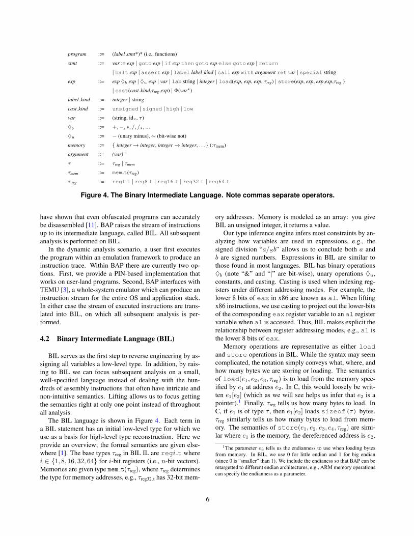
program ::= (label stmt*)* (i.e., functions)

stmt ::= var := exp | goto exp | if exp then goto exp else goto exp | return| halt exp | assert exp | label label kind | call exp with argument ret var | special string

exp ::= exp ♦b exp | ♦u exp | var | lab string | integer | load(exp, exp, exp, τreg) | store(exp, exp, exp,exp,τreg )

| cast(cast kind,τreg,exp) | Φ(var∗)

label kind ::= integer | string

cast kind ::= unsigned | signed | high | lowvar ::= (string, idv , τ )

♦b ::= +,−, ∗, /, /s, ...♦u ::= − (unary minus), ∼ (bit-wise not)

memory ::= { integer→ integer, integer→ integer, . . .} (:τmem)

argument ::= (var)+

τ ::= τreg | τmem

τmem ::= mem t(τreg)

τ reg ::= reg1 t | reg8 t | reg16 t | reg32 t | reg64 t

Figure 4. The Binary Intermediate Language. Note commas separate operators.

have shown that even obfuscated programs can accuratelybe disassembled [11]. BAP raises the stream of instructionsup to its intermediate language, called BIL. All subsequentanalysis is performed on BIL.

In the dynamic analysis scenario, a user first executesthe program within an emulation framework to produce aninstruction trace. Within BAP there are currently two op-tions. First, we provide a PIN-based implementation thatworks on user-land programs. Second, BAP interfaces withTEMU [3], a whole-system emulator which can produce aninstruction stream for the entire OS and application stack.In either case the stream of executed instructions are trans-lated into BIL, on which all subsequent analysis is per-formed.

4.2 Binary Intermediate Language (BIL)

BIL serves as the first step to reverse engineering by as-signing all variables a low-level type. In addition, by rais-ing to BIL we can focus subsequent analysis on a small,well-specified language instead of dealing with the hun-dreds of assembly instructions that often have intricate andnon-intuitive semantics. Lifting allows us to focus gettingthe semantics right at only one point instead of throughoutall analysis.

The BIL language is shown in Figure 4. Each term ina BIL statement has an initial low-level type for which weuse as a basis for high-level type reconstruction. Here weprovide an overview; the formal semantics are given else-where [1]. The base types τreg in BIL IL are regi t wherei ∈ {1, 8, 16, 32, 64} for i-bit registers (i.e., n-bit vectors).Memories are given type mem t(τreg), where τreg determinesthe type for memory addresses, e.g., τreg32 t has 32-bit mem-

ory addresses. Memory is modeled as an array: you giveBIL an unsigned integer, it returns a value.

Our type inference engine infers most constraints by an-alyzing how variables are used in expressions, e.g., thesigned division “a/Sb” allows us to conclude both a andb are signed numbers. Expressions in BIL are similar tothose found in most languages. BIL has binary operations♦b (note “&” and “|” are bit-wise), unary operations ♦u,constants, and casting. Casting is used when indexing reg-isters under different addressing modes. For example, thelower 8 bits of eax in x86 are known as al. When liftingx86 instructions, we use casting to project out the lower-bitsof the corresponding eax register variable to an al registervariable when al is accessed. Thus, BIL makes explicit therelationship between register addressing modes, e.g., al isthe lower 8 bits of eax.

Memory operations are representative as either loadand store operations in BIL. While the syntax may seemcomplicated, the notation simply conveys what, where, andhow many bytes we are storing or loading. The semanticsof load(e1, e2, e3, τreg) is to load from the memory spec-ified by e1 at address e2. In C, this would loosely be writ-ten e1[e2] (which as we will see helps us infer that e2 is apointer).1 Finally, τreg tells us how many bytes to load. InC, if e1 is of type τ , then e1[e2] loads sizeof(τ) bytes.τreg similarly tells us how many bytes to load from mem-ory. The semantics of store(e1, e2, e3, e4, τreg) are simi-lar where e1 is the memory, the dereferenced address is e2,

1The parameter e3 tells us the endianness to use when loading bytesfrom memory. In BIL, we use 0 for little endian and 1 for big endian(since 0 is “smaller” than 1). We include the endianess so that BAP can beretargetted to different endian architectures, e.g., ARM memory operationscan specify the endianness as a parameter.

6

and the value written in e3. store syntactically returns anew memory name indicating that an update has happened,which is used extensively when we translate BIL to singlestatic assignment (SSA) form (§5.1).Statements and Programs. A program in BIL is a labelfollowed by a sequence of statements. For example, in thestatic case the label is the beginning of the function andthe statements are the lifted assembly. Every function im-plicitly takes as arguments the current set of registers andthe current state of memory, each of which may be typed.BIL statements are straight-forward: there are statementsfor assignments, jumps, conditional jumps, and labels. Inaddition, we include special statements to identify in-vocation points for externally defined procedures and func-tions, e.g., int 0x80 is translated to special. The id ofa special indexes the kind of special, e.g., what systemcall, which is used in subsequent analysis. As we will see,if we know the types of a system call, we can use that infor-mation to infer high-level types.

5 Variable Recovery

5.1 Static Single Assignment (SSA)

High-level languages typically allow an arbitrary num-ber of variables, each of which must be assigned to a fixednumber of registers (e.g., the 6 general purpose registerson x86). Further, stack slots may be reused for differentvariables of different types, thus we may need to deconflictwhen multiple variables are given to a single stack slot. 2

TIE’s first step in variable recovery is to deconflict dif-ferent uses of the same register and memory cells by trans-forming the BIL program into single static assignment form(SSA). SSA on registers is performed by giving each newregister assignment a unique name. For example, each timeeax is assigned a value we will invent a new instance nameeax1, eax2, etc. Note SSA deconflicts multiple writes tothe same register; it does not recover the original variablenames as that information is lost during compilation.

While SSA on scalar registers is quite common,we also put memory into SSA, e.g., the x86 in-struction mov [eax], 0xaabbccdd is written asmem1 = store(mem0, eax, 0xaabbccdd, 0,reg32 t). During type reconstruction, having differentnames allows us to type a stack slot in mem0 differentthan mem1. This feature improves our accuracy since asingle stack slot may be used for many different variableinstances, e.g., when designated as a generic register spillduring the register allocation compilation phase [4].

If a variable v is updated in two different branches, thevariable has a different instance v1 and v2 for each branch.

2An example of when a single stack slot is used for different variablesis when the variables have disjoint live ranges.

When the branches meet, we need to give a unique name tosubsequent references regardless of which branch was exe-cuted. This is denoted by introducing a φ function at eachbranch confluence point, e.g., v3 = Φ(v1, v2).

5.2 DVSA Algorithm

The variable recovery algorithm DVSA takes in the pro-gram in SSA form, and outputs variable locations in mem-ory along with alias information. The candidate variablesare later typed, and the alias information is used to deter-mine when a single memory slot is used for two differenttypes.

A variable is represented as a symbolic memory load orstore. We determine the variables by building up a conser-vative estimate of the memory configuration by analyzingSSA memory operations. For example, the BIL statementsshown in Figure 3(a) show the SSA form of our runningexample. We generate a map that shows mem0 has mem-ory configuration {t1 → ebp0}, mem1 has configuration{t2 → 0} ∪ mem0, etc. For straight-line code, each newmemory state will be derived from exactly one previousmemory state. However, with control flow we must con-sider memory at merge points, e.g., the memory state afteran if-then-else is the confluence of all paths. For controlflow we consider all the confluence of all possible memo-ries, e.g., if there is an update to t1 with value v1 along path1 and an update along path 2 with value v2, we say thatt1 → {v1, v2}.

We use a variant of Value Set Analysis (VSA) [5] todetermine possible alias relationships in subsequent steps.VSA is an assembly code abstraction interpretation analysisthat approximates the range of values a variable may take onas a strided interval (SI). SI has a form of s[lb, ub], wheres is a stride and [lb, ub] is the interval, the lower and upperbound of the value. For example, the SI 2[0, 10] representsthe set {0,2,4,6,8,10}. Strided intervals are more specificthan simple ranges. However, they over-approximate theset of possible values, e.g., the SI for set {1,2,4} is 1[1, 4],which is an over-approximation since this SI represents theset {1,2,3,4}. The main difference between our variant andthe original VSA [5] is we generalize VSA to create anSI based upon linear combinations of scalars. The origi-nal VSA would implicitly define the SI as being with re-spect to a single reference register, e.g., ebp. We allow forVSA to include any combination of scalar variables in ourSSA form. This leads to more accurate results in our exper-iments. More details about the specifics of our algorithmcan be found elsewhere [8].

7

T ::= τ data | τ fun | > | ⊥ | T ∩ T | T ∪ T | T → T

τ data ::= τ base | τ mem

τ base ::= τ reg | τ refined

τ reg ::= reg1 t | reg8 t | reg16 t | reg32 t

τ refined ::= numn t | uintn t | intn t (n = 8,16, 32) |ptr(T ) | code t

τ mem ::= {∀ addresses i|li : Ti}τ R ::= {var1 : T1, · · · , varn : Tn}τ fun ::= τ mem → τ R → T

constraints ::= T = T | T <: T

| constraints ∧ constraints

| constraints ∨ constraints

Figure 5. Types and constraints of TIE

6 TIE: Type Inference on Binary Code

6.1 Type System

The input to the type reconstruction phase of TIE is theBIL code annotated with simple register types. Type recon-struction in TIE is the process of collecting and analyzinghints based upon how binary operations treat variables inorder to infer high-level types. We use subtype theory to ex-press the amount of uncertainty that may exist on the exacthigher-level type of a variable. For example, we may knowthat a variable is used as an integer, but not know whether itis signed or not. In our system we have a number supertypewhich is less specific than either a signed or an unsignedinteger.

TIE enriches the basic binary-code types from BIL toinclude:

• >, which corresponds to a variable being “any” type,and ⊥, which corresponds to a variable being used ina type-inconsistent manner.• Numbers (numn t), signed integers (intn t), and

unsigned integers (uintn t).• Pointers of type ptr(T) where T is some other type

in the system.• Records of a fixed number of variables, which map the

variable name vari to its type Ti. We also distinguishthe memory type τmem, which maps each memory celladdress to the type stored at that address.• General function types T1 → T2. In addition, we de-

note by τfun the type for high-level C functions we in-fer, which takes the current memory state and a list ofregisters as arguments, and returns something of typeT .• Intersection types (T ∩ T ) and union types (T ∪ T ),

reg32_t

num32_t ptr(α)

⊥

⊥

int32_t uint32_t

reg16_t

num16_t

int16_t uint16_t

reg8_t reg1_t

num8_t

int8_t uint8_t

code_t

Figure 6. Type lattice showing the hierarchyof types in τ base

which we explain below.

The base integer types in TIE form a subtyping lattice,shown in Figure 6. We omit additional edges betweenbase types to keep the diagram simple, e.g., reg16 t <:reg32 t, though they do exist in our type system. Thesubtyping relationships are extracted from the lattice as fol-lows: if S ← T is an edge in the lattice, then S <: T (i.e.,think of “<:” as an arrow in the lattice). Following multipleedges in the lattice corresponds to the transitive nature ofsubtyping. Since a type hierarchy is a lattice, the u and toperations are also applied in the context of subtyping, e.g.,T1uT2 = M where M is the greatest lower bound of typesT1 and T2 in the subtyping hierarchy.

Intersection and Union Types. TIE’s type system has in-tersection (∩) and union (∪) types. Mathematically, some-thing is of type T1 ∩ T2 if it can be described by both types,e.g., if T1 is the C type for signed characters of range -128to 127 and T2 is the C type for unsigned characters of range0 to 255, then T1 ∩ T2 is the type for range 0 to 127. Inour type system, we use intersection types during constraintsolving where something is of type T1∩T2 if it is the order-theoretic meet (i.e., greatest lower bound) of T1 u T2.

The dual of intersection types is union type T1 ∪ T2,corresponding to the order-theoretic join (i.e., lowest upperbound) T1 t T2. The values of T1 ∪ T2 include the unionof values from both types. Note that union types are not thesame as sum types. A sum type adds a tag, while a uniontype extends the range of values.

Output. The output of type inference is an upper andlower bound on the type for each variable. The user is thenfree to pick either as the inferred type. Of course if wecan completely infer the type we output the same type forthe upper and lower bound. However, outputting a range ismuch more general, and can make explicit the uncertaintydue to the nature of the problem. For example, C unionsmay be compiled down so that a single stack slot holds dif-

8

C types Corresponding types in our type system

int int32 t

unsigned int uint32 t

short int int16 t

unsigned short int uint16 t

char int8 t

unsigned char uint8 t

* (pointer) ptr(α)

void * ptr(>)

void ⊥union T ∪ T

struct, [] (array) {li : Ti}function τ mem → R→ T (:τ fun)

Table 1. Mapping between the C types thetypes in our type system.

ferent typed variables. The only reason we know the typeof the variable at any point in time is due to a user annota-tion, which is completely lost during compilation. Our typesystem allows us to express such uncertainty by expressingone bound as a type conflict(⊥) and one as a C union (∪).

Correspondence to C Types. TIE’s type system containsfeatures of modern programming languages which are thentranslated in a post-processing step to types in a specificlanguage. Currently TIE is targeted to output C types bytranslating internally-inferred TIE types into C types usingthe translation shown in Table 1. Structure types in C cor-respond to record types in our language, as expected. Thevoid and void * rules may seem strange for those unfamiliarwith typing systems. It may seem that void * is a pointer tovoid, however this is an unfortunate naming problem in C.void corresponds to no type which is why we equate it with⊥ in our system. 3 void * can point to anything at all, whichis why we equate it to ptr(>).

Evaluation Metrics. Our goal is to infer conservative yetaccurate types. Conservativeness means we want to infer nomore than the binary code tells us, e.g., never guess a type.In addition, we want to be precise by inferring as much aspossible from the code.

More formally, let τt be a type variable for a term t.We allow a typing algorithm to output both a lower boundB↓(τt) and an upper bound B↑(τt) for a variable. If thetyping algorithm wants to indicate a specific type it outputsτ = B↓(τt) = B↑(τt).

An algorithm is conservative if the real type τ for a pro-gram is between the upper and lower bound. More formally:

3Another option would be to introduce the unit type. We did not seeany advantage in doing so.

Definition 6.1. [CONSERVATIVENESS] For a term t, let τsrcbe the type of t in the source code. Given a well-typedsource code program, we say a typing algorithm for t isconservative with respect to the real type of t (τsrc) if

B↓(τt) <: τsrc <: B↑(τt).

Being conservative is desirable, but not sufficient. Forexample, an algorithm could output > for the upper boundand ⊥ as a lower bound and always be conservative. There-fore, we also define the notion of how precise the inferredtype is by measuring the distance between the upper andlower bound. For example, if an algorithm outputs the sameupper and lower bound, and the output type is the same asthe source code type, the distance is 0 and the algorithm iscompletely precise.

The distance is measured with respect to our type lattice.If two types can form a type interval, i.e., one is a subtypeof the other, their distance is the number of edges separatingthem on the lattice. If the two types are incompatible, theirdistance is set to the maximum value. More formally, thedistance between types is defined as:

Definition 6.2. [DISTANCE] For two types, τ1 and τ2, thedistance between them, denoted by ||τ1 − τ2||, is the differ-ence between the level of each in the type lattice if τ1 <: τ2or τ2 <: τ1. Otherwise, it is the maximum distance, whichis ||> − ⊥||.

In our type system shown in Figure 6, the maximumvalue of ||> − ⊥|| is 4.

Structural types. Our accuracy metric handles structuresas two dimensions in terms of distance: how many fieldswere inferred vs. the real number of fields, and the distancebetween the real type for a field and its inferred type.

We formalize the distance between two structure typesA = {li : Si∈1..nA

i } and B = {li : T i∈1..nBi } as ||A − B||

by measuring the difference between the number of fieldsand type for each field:

||A−B|| =∣∣∣∣(1− 1

nA)− (1− 1

nB)

∣∣∣∣+ avg||Si − T i∈1..max(nA,nB)i ||||⊥ − >|| ,

(1)where nA and nB denote the number of fields for A and B,respectively. The first term shows the difference in the num-ber of fields and the second term measures the distance ofeach field element using the subtype relation. Note that, tobe compatible with the levels in the type lattice the distancesare normalized over the total lattice height.

For example, suppose two record types U = {0 :int32 t} and V = {0 : int32 t, 4 : uint32 t}. Thenumber of fields nU and nV are 1 and 2, respectively. Thus,||U − V || = |(1− 1

1 )− (1− 12 )|+ (0+4)/2

4 = 1. In addition,||reg32 t−V || is computed as the difference of the levelsof reg32 t and V , which is ||reg32 t−{0 : >}||+ ||{0 :>} − V || = 1 + 1.5 = 2.5.

9

Statement Generated constrains

x := e τx = τe

goto e τe = ptr(code t)

if e then goto et else goto ef τe = reg1 t ∧ τt = ptr(code t) ∧ τf = ptr(code t)

call f withm v∗ ret r τ ′m = τmf ∧∧v(τv = τvf .[v]) ∧ τr = τrf

(where F ` f : τmf → τvf → τrf , τ ′m = #update(τm))

Expression Generated constraint for term with type variable τ

x (variable) τx

v (integer) τv

−ne (unary neg) τe <: intn t ∧ τ :> intn t

e1 +32 e2 (τe1 <: Tγ ∧ τe2 <: Tγ ∧ τ :> Tγ ∧ Tγ <: num32 t)

∨(τe1 <: ptr(Tα) ∧ τe2 <: num32 t ∧ τ :> ptr(Tβ))

∨(τe1 <: num32 t ∧ τe2 <: ptr(Tα) ∧ τ :> ptr(Tβ))

e1 +n6=32 e2 τe1 <: Tγ ∧ τe2 <: Tγ ∧ τ :> Tγ ∧ Tγ <: numn t

∼n e τe <: uintn t ∧ τ :> uintn t

e1 <Sn e2 τe1 <: intn t ∧ τe2 <: intn t ∧ τ :> reg1 t

load(m, i, d,regn t) τi = ptr(τm.[i]) ∧ τ = τm.[i] ∧ τ <: regn t

store(m, i, v, d,regn t) τi = ptr(τv) ∧ τ = τm{i : τv} ∧ t.[i] <: regn t

Φ(e1, · · · , en) τ ′ <: τe1 ∩ · · · ∩ τen

Figure 7. Example rules for type constraint generation

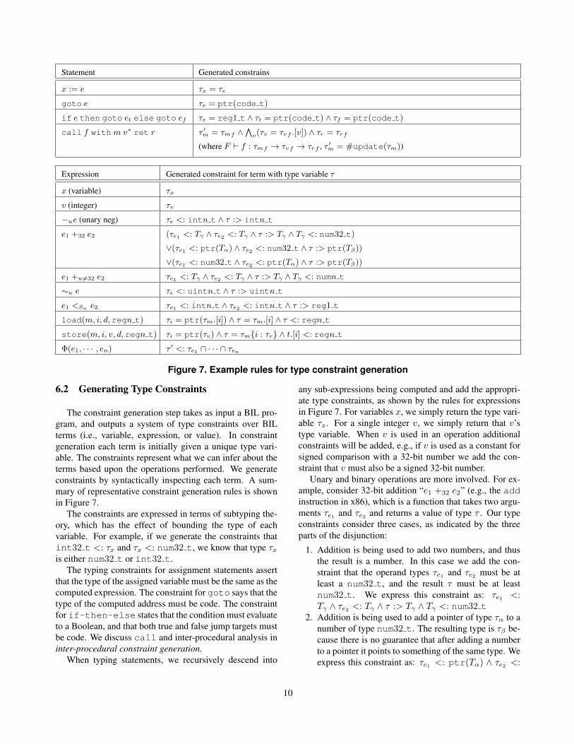
6.2 Generating Type Constraints

The constraint generation step takes as input a BIL pro-gram, and outputs a system of type constraints over BILterms (i.e., variable, expression, or value). In constraintgeneration each term is initially given a unique type vari-able. The constraints represent what we can infer about theterms based upon the operations performed. We generateconstraints by syntactically inspecting each term. A sum-mary of representative constraint generation rules is shownin Figure 7.

The constraints are expressed in terms of subtyping the-ory, which has the effect of bounding the type of eachvariable. For example, if we generate the constraints thatint32 t <: τx and τx <: num32 t, we know that type τxis either num32 t or int32 t.

The typing constraints for assignment statements assertthat the type of the assigned variable must be the same as thecomputed expression. The constraint for goto says that thetype of the computed address must be code. The constraintfor if-then-else states that the condition must evaluateto a Boolean, and that both true and false jump targets mustbe code. We discuss call and inter-procedural analysis ininter-procedural constraint generation.

When typing statements, we recursively descend into

any sub-expressions being computed and add the appropri-ate type constraints, as shown by the rules for expressionsin Figure 7. For variables x, we simply return the type vari-able τx. For a single integer v, we simply return that v’stype variable. When v is used in an operation additionalconstraints will be added, e.g., if v is used as a constant forsigned comparison with a 32-bit number we add the con-straint that v must also be a signed 32-bit number.

Unary and binary operations are more involved. For ex-ample, consider 32-bit addition “e1 +32 e2” (e.g., the addinstruction in x86), which is a function that takes two argu-ments τe1 and τe2 and returns a value of type τ . Our typeconstraints consider three cases, as indicated by the threeparts of the disjunction:

1. Addition is being used to add two numbers, and thusthe result is a number. In this case we add the con-straint that the operand types τe1 and τe2 must be atleast a num32 t, and the result τ must be at leastnum32 t. We express this constraint as: τe1 <:Tγ ∧ τe2 <: Tγ ∧ τ :> Tγ ∧ Tγ <: num32 t

2. Addition is being used to add a pointer of type τα to anumber of type num32 t. The resulting type is τβ be-cause there is no guarantee that after adding a numberto a pointer it points to something of the same type. Weexpress this constraint as: τe1 <: ptr(Tα) ∧ τe2 <:

10

num32 t ∧ τ :> ptr(Tβ)3. Addition is being used to add an integer of type

num32 t to a pointer of type τα. This case is sym-metric to the above.

Unary negation (−n), bitwise complementing (∼n),arithmetic operations on variables other than 32-bits, andsigned operations allow us to be much more specific in theconstraints generated. For example, unary negation andsigned comparison allow us to infer that the types of theoperands are at least of signed type. Note that the subtyperelation is covariant for the result type τ and contravari-ant for the operand types since binary and unary operationsare functions with specific types, e.g., −n : intn t →intn t.

Typing Memory Operations. Recall we model memoryas an array of elements indexed by an address. We denoteby [i] the DVSA value of i. The typing rules for loadand store should propagate types so that if we store avalue of type α at address [i1], and then subsequently loada value from [i2], then the resulting type is α when [i1] =[i2]. We first describe how the typing rules express this idea,and then discuss how equality between symbolic values iscalculated.

The load rule states that when we are given an indexi into memory m, then i) we can treat the type of i like apointer to the type of values at m.[i], and ii) the returnedtype τ is the same as the type of values stored at m.[i], andiii) since the load was t bytes, the resulting type must be asubtype of t (i.e., τ <: reg32 t for a 32-bit load). Thestore operation is symmetric: if we are storing a value v oftype τv at [i], then the memory cell at [i] has type τv .

We introduce equality constraints between memorydereferences when the DVSA SI’s overlap. For example,if we store to address j and load from address i, and theDVSA SI’s say that j and i are the same address range, weadd a type constraint between the referenced memory cells.This is imprecise and possibly un-conservative, e.g., if j’saddress range is from [0, 100] and i’s address range is [2, 4],then the load from i may completely, partially or not at alloverlap. As we show in our evaluation our conservativenessin practice is typically above 90% even with such issues.

Inter-procedural constraint generation. As a pre-processing step, we create a context F of type signaturesfor known functions such as those in libc. When a call to afunction f is issued, we first search the function descriptionfor the function f in F . If we find a function description(τmf → τvf → τrf ) for the function from F , we match itcaller’s type variables for arguments and return value. Thefunction #update(τ mem) uses information about callingconventions to match up offsets correctly. For example, inthe standard call of 32-bit x86 architecture, #update up-dates {li 7→ Ti} to {li + esp− ebp + 4 7→ Ti}.

struct bar {char *name;int size;

};struct bar m;struct bar *p = &m;p->size = 10;

p

name : Tαsize : Tβ

points

+4 {0 : Tα, 4 : Tβ}

Ptr {0 : Tα, 4 : Tβ}

m

Figure 8. Access to structural data (sourcecode and stack)

TIE also handles calls to functions without known pa-rameter types, e.g., when one local procedure calls anotherlocal procedure. During pre-processing TIE adds all func-tion names to F . When a call is made to a function, TIEmatches up the callers arguments with the number of pa-rameters inferred for the callee during DVSA. TIE then addsthe appropriate equality constraints, e.g., the type of the firstpassed argument must be the same as the first parameter.This process is dependent on calling conventions and plat-form. For example, in the standard call of 32-bit x86 ar-chitecture, we follow the memory access with the addressabove ebp, such as ebp + 4 or ebp + 8, to find the num-ber and variables for the arguments, and the last value ofeax will be the return value. Supporting additional callingconventions is straight-forward, e.g., adding fastcall wouldentail adding constraints that the first two arguments arepassed in ecx and edx.

Constraints for structural data. To infer the type ofstructural data, we restate the rules in Figure 7. Binaryprograms access the structural data in two ways: 1) accessvia pointers, where binary programs calculate the addressof fields by arithmetic operations on the base pointer, and2) direct access, where the structural data reside in the stackas multiple variables, and the fields are accessed directly.Unfortunately, directly accessing structure fields is indis-tinguishable from accessing local variables on the stack.Therefore, we use the access via pointers as a hint that re-veals the presence of structural data.

Figure 8 gives the intuition of constraint generation forstructural data. A variable m of a two-field structure baris located on the stack and a pointer p points to m. Whenthe second field size is accessed through p, its addressis calculated by applying an add operation with pointer p.Thus, we can tell that p points to structural data, which hasat least one field at offset 4.

To handle constraints for such hints, we redefine the rulesfor e1 +32 e2. If a pointer is used in addition with a constantvalue, we infer it as a pointer to structural data as follows.

(τe1 <: Tγ ∧ τe2 <: Tγ ∧ τ :> Tγ ∧ Tγ <: num32 t)

∨(τe1 <: ptr({0 : Tα, [e2] : Tβ}) ∧ τe2 <: num32 t ∧ τ :> ptr(Tβ))

∨(τe1 <: num32 t ∧ τe2 <: ptr({0 : Tα, [e1] : Tβ}) ∧ τ :> ptr(Tβ)),

11

where [e1] and [e2] are the value of e1 and e2, respectively.For example, the constraint generated for p is (we show the2nd disjunctive constraint) · · · ∨ (τp <: ptr({0 : Tα, 4 :Tβ}) ∧ τ4 <: num32 t ∧ τ :> ptr(Tβ)) ∨ · · · .

6.3 Constraint Solving

The final step in TIE is solving the generated type con-straints. In this section we present our constraint solving al-gorithm, that takes in a list of type constraints C and returnsa map from type variables to the inferred type interval. Weuse a unification algorithm extended to support subtypes.During the constraint solving process, we keep a workingset that contains the current state of our algorithm. Theworking set consists of the following:• C: the list of type constraints that remain to be pro-

cessed by our algorithm.• S<:: a set containing all the inferred subtype relations.• S=: a map from bound type variables to types.• B↑: a map from type variables to the upper bound of

the inferred type.• B↓: a map from type variables to the lower bound of

the inferred type.

The final solution returns the pair 〈B↑,B↓〉. During eachstep of constraint solving, we remove and process a singleelement from the constraint worklist C. Our algorithm ter-minates when the constraint list is empty (C = ∅). Theinitial constraint list contains the constraints from the con-straint generation process (described in § 6.2) while all othercontexts (S<:, S=, B↑, B↓) are initialized to empty (∅).

In sections § 6.3.3-§ 6.3.4 we describe how we solve eachconstraint type shown in Figure 5. We solve each constraintin the following order: equality, subtype relation, conjunc-tive and disjunctive constraints.

6.3.1 Equality constraints (Tα = Tβ)

Equality constraints are solved through unification. Unifica-tion is essentially a substitution process, where given S = Twe replace all occurrences of S with T in our worklist C.Algorithm 1 shows how the working set is updated for everyequality constraint.

Note that before performing substitution, we perform theoccurs check [17], in which we check whether a type vari-able occurs in both hands of an equality, e.g., α = ptr(α).Since we do not support recursive types, we raise type er-ror and drop the current working set whenever we have anoccurs check violation. Also note that the last option in ouralgorithm is to drop the constraint. We do this to continuetyping the remaining variables, instead of failing and return-ing the type ⊥ for all variables.

6.3.2 Subtype relation constraints (Tα <: Tβ)

To solve subtype relation constraints, we use a type closurealgorithm. Subtype relation constraints describe type in-

Algorithm 1: Solving a single equality constraint fromthe constraint list C.SolveEquality (S = T , C)

if IsFreeVariable(S) thenC = C[S\T ] ; S= = S={S 7→ T} ;

else if IsFreeVariable (T ) thenC = C[T\S] ; S= = S={T 7→ S} ;

else if S = ptr(S1) and T = ptr(T1) thenC = C ∪ {S1 = T1} ;

else if S = {li : Si} and T = {li : Ti} thenC = C ∪

⋃i{Si = Ti} ;

elseDrop Constraint

end

equality relations, thus the solution provided by the closurealgorithm maps each type variable to an interval. For eachtype variable α, we keep track of its upper bound B↑(α)and lower bound B↓(α), which are initialized as > and ⊥,respectively. Every time we process a subtype relation con-straint that involves a type α, the closure algorithm usesthe constraint to refine the type interval of α. For exam-ple, the constraint α <: ptr(int32 t) makes the closurealgorithm update the upper bound of α to ptr(int32 t)(B↑(α)← ptr(int32 t)).

The core idea behind the closure algorithm is the prop-agation of type information via transitive subtype relations.We use S<:, to keep track of the transitive subtype rela-tion. S<: is always closed under the subtype relation for agiven set of subtype relation constraints. For example, ifS<: = {α <: β} and we append the constraint β <: γ,the new S<: will become {α <: β, β <: γ, α <: γ}.If another constraint int32 t <: α is given, the lowerbound of α, β, γ will be updated to int32 t. Note that forconstraints on constructed types, e.g., ptr(α) <: ptr(β)we recurse into the ptr() and infer the implicit constraintsα <: β.

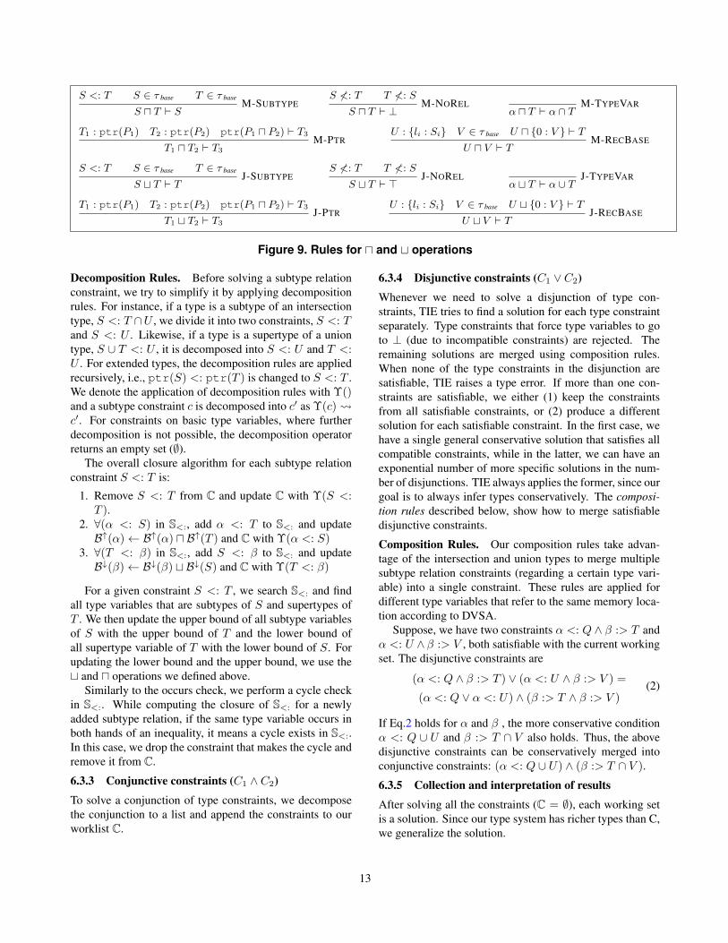
Meet and Join. We populate B↑ and B↓ during the sub-type resolution process. We define rules for u and t op-erations in Figure 9 to compute the upper bound B↑ andlower bound B↓ respectively. M-SUBTYPE and M-NORELshow the basic behavior of the u operation. As shown inM-TYPEVAR, if u is applied with a type variable α, it pro-duces the intersection type with α. In M-PTR, we applyu on the parameters of pointers, recursively. For the en-tries that have no matched label in both record types, weadd them to the result of u. As shown in M-RECBASE, if arecord type meets a base type τ , then the base type is con-verted to an equivalent record type {0 : τ}, and u is appliedto them again. The rules for t work in a similar manner.

12

S <: T S ∈ τ base T ∈ τ base

S u T ` SM-SUBTYPE

S 6<: T T 6<: S

S u T ` ⊥M-NOREL

α u T ` α ∩ TM-TYPEVAR

T1 : ptr(P1) T2 : ptr(P2) ptr(P1 u P2) ` T3

T1 u T2 ` T3

M-PTRU : {li : Si} V ∈ τ base U u {0 : V } ` T

U u V ` TM-RECBASE

S <: T S ∈ τ base T ∈ τ base

S t T ` TJ-SUBTYPE

S 6<: T T 6<: S

S t T ` >J-NOREL

α t T ` α ∪ TJ-TYPEVAR

T1 : ptr(P1) T2 : ptr(P2) ptr(P1 u P2) ` T3

T1 t T2 ` T3

J-PTRU : {li : Si} V ∈ τ base U t {0 : V } ` T

U t V ` TJ-RECBASE

Figure 9. Rules for u and t operations

Decomposition Rules. Before solving a subtype relationconstraint, we try to simplify it by applying decompositionrules. For instance, if a type is a subtype of an intersectiontype, S <: T ∩U , we divide it into two constraints, S <: Tand S <: U . Likewise, if a type is a supertype of a uniontype, S ∪ T <: U , it is decomposed into S <: U and T <:U . For extended types, the decomposition rules are appliedrecursively, i.e., ptr(S) <: ptr(T ) is changed to S <: T .We denote the application of decomposition rules with Υ()and a subtype constraint c is decomposed into c′ as Υ(c) c′. For constraints on basic type variables, where furtherdecomposition is not possible, the decomposition operatorreturns an empty set (∅).

The overall closure algorithm for each subtype relationconstraint S <: T is:

1. Remove S <: T from C and update C with Υ(S <:T ).

2. ∀(α <: S) in S<:, add α <: T to S<: and updateB↑(α)← B↑(α) u B↑(T ) and C with Υ(α <: S)

3. ∀(T <: β) in S<:, add S <: β to S<: and updateB↓(β)← B↓(β) t B↓(S) and C with Υ(T <: β)

For a given constraint S <: T , we search S<: and findall type variables that are subtypes of S and supertypes ofT . We then update the upper bound of all subtype variablesof S with the upper bound of T and the lower bound ofall supertype variable of T with the lower bound of S. Forupdating the lower bound and the upper bound, we use thet and u operations we defined above.

Similarly to the occurs check, we perform a cycle checkin S<:. While computing the closure of S<: for a newlyadded subtype relation, if the same type variable occurs inboth hands of an inequality, it means a cycle exists in S<:.In this case, we drop the constraint that makes the cycle andremove it from C.

6.3.3 Conjunctive constraints (C1 ∧ C2)

To solve a conjunction of type constraints, we decomposethe conjunction to a list and append the constraints to ourworklist C.

6.3.4 Disjunctive constraints (C1 ∨ C2)

Whenever we need to solve a disjunction of type con-straints, TIE tries to find a solution for each type constraintseparately. Type constraints that force type variables to goto ⊥ (due to incompatible constraints) are rejected. Theremaining solutions are merged using composition rules.When none of the type constraints in the disjunction aresatisfiable, TIE raises a type error. If more than one con-straints are satisfiable, we either (1) keep the constraintsfrom all satisfiable constraints, or (2) produce a differentsolution for each satisfiable constraint. In the first case, wehave a single general conservative solution that satisfies allcompatible constraints, while in the latter, we can have anexponential number of more specific solutions in the num-ber of disjunctions. TIE always applies the former, since ourgoal is to always infer types conservatively. The composi-tion rules described below, show how to merge satisfiabledisjunctive constraints.

Composition Rules. Our composition rules take advan-tage of the intersection and union types to merge multiplesubtype relation constraints (regarding a certain type vari-able) into a single constraint. These rules are applied fordifferent type variables that refer to the same memory loca-tion according to DVSA.

Suppose, we have two constraints α <: Q ∧ β :> T andα <: U ∧ β :> V , both satisfiable with the current workingset. The disjunctive constraints are

(α <: Q ∧ β :> T ) ∨ (α <: U ∧ β :> V ) =

(α <: Q ∨ α <: U) ∧ (β :> T ∧ β :> V )(2)

If Eq.2 holds for α and β , the more conservative conditionα <: Q ∪ U and β :> T ∩ V also holds. Thus, the abovedisjunctive constraints can be conservatively merged intoconjunctive constraints: (α <: Q ∪ U) ∧ (β :> T ∩ V ).

6.3.5 Collection and interpretation of results

After solving all the constraints (C = ∅), each working setis a solution. Since our type system has richer types than C,we generalize the solution.

13

1

1.5

2

2.5

3

0 10 20 30 40 50 60 70 80

Type

inte

rval

leng

th

Number of programs

TIE w/ inter-procedural analysisTIE w/o inter-procedural analysis

(a) Precision

-0.4

-0.2

0

0.2

0.4

0 10 20 30 40 50 60 70 80

Posi

tion

of re

al ty

pes

with

in ty

pe in

terv

al

Number of programs

TIE w/ inter-procedural analysisTIE w/o inter-procedural analysis

(b) Conservativeness rateFigure 10. Summary of precision (left) and conservativeness (right)

Type interval. In the working set, the upper bound andlower bound provide the range of the inferred type for thevariable. We call the interval from the lower bound to theupper bound of a variable α as a “type interval,” denoted by[B↓(α),B↑(α)].

Structural equality in results. The real types in C sourcecodes has struct and arrays for structural types. However,pointers are also used interchangeably with them. Thus, thethree types are not distinguishable because their behavior isthe same in binary programs. In our type system, we assumethey are in structural equivalence as follows:

ptr(α) ≡ {0 7→ α} ≡ α[](array)

When we compare two structural equivalent types. We con-vert the type into a record type {0 7→ α}, which is the mostgeneral form.

Collection and generalization. We convert each work-ing set into a final solution. First, if a type variable, Tα,is remained in B↑ and B↓, we replace it as B↑(Tα) in B↑and B↓(Tα) in B↓, respectively. We also generalize recordtypes. If B↑ of record types has fields of >, we remove thefields. If all the fields in B↑ are of the same type, {li : T ∀i},we convert it to more general structure form, {0 : T}, ac-cording to the structural equivalence. Second, for each termt, we find a matching type variable Tt and a type intervalof [B↓(α),B↓(α)]. If S= has a mapping for Tt, we usethe equivalent type variable of Tt in S= instead of Tt. Atlast, we collect the result for memory and group them byits address. Since we are based on the SSA form, we mayhave more than one variable for each memory address andit means the memory location is reused by various data ofdifferent type. Thus, we combine members for the sameaddress as a union type of them. Through this collectionprocess, each variable has a final type interval.

7 Implementation

TIE is primarily implemented in 29k of OCaml code,most of which is generic binary analysis code such as adata-flow framework, building CFG’s, etc. Our static anal-ysis component uses a linear sweep disassembler writtenin C build on top of libopcodes (more advanced disas-sembly such as dealing with obfuscated code is left outsidethe scope of this paper, but such routines can be pluggedinto our infrastructure). We base our dynamic analysis onPIN [13], and currently there are about 1.4k lines of C++code to create the instruction trace. The variable recoveryand type inference are approximately 3.6 and 2.1K lines ofOCaml, respectively.

8 Evaluation

8.1 Evaluation Setup

We have evaluated TIE on 87 programs fromcoreutils (v8.4). We compiled the programs with de-bug support but only use the information for measuring typeinference accuracy. The type information was extracted us-ing libdwarf. TIE’s inter-procedural analysis used func-tion prototypes for libc, as extracted from the appropriateheader files. All experiments are performed on 32-bit x86binaries in Linux.

We measure the accuracy of TIE against the RE-WARDS [12] code given to use by the authors for the dy-namic analysis setting, and against Hex-rays decompiler(v1.2) in IDA Pro [2] for static analysis setting.

TIE outputs an upper and lower bound on the inferredtype. We use this to measure the conservativeness of TIE.For precision, we translate the bound output by TIE into asingle C type by translating the lower bound unless it is ⊥.If the lower bound is ⊥, we output the upper bound. Wefound this heuristic to provide the most accurate results.

14

0

0.2

0.4

0.6

0.8

1

0 10 20 30 40 50 60 70 80

Cum

ulat

ive

aver

age

rate

of c

onse

vativ

e ty

pes

Number of programs

Hex-raysTIE w/ inter-procedural analysis

TIE w/o inter-procedural analysis

(a) Conservativeness for structural types.

0

0.5

1

1.5

2

2.5

3

0 10 20 30 40 50 60 70 80

Cum

ulat

ive

aver

age

dist

ance

Number of programs

Hex-raysTIE w/o inter-procedural analysis

TIE w/ inter-procedural analysis

(b) Distance for structural types.

Figure 11. Conservativeness and distance for structural types

Caveats. Hex-rays and REWARDS have an inherentlyless informative type system than ours since they are re-stricted to only C types. For example, REWARDS guessesthat a register holds an uint32 t with no additionalinformation for 32-bit registers, while Hex-rays guessesint32 t in the same situation. Our reg32 t reflects inthe same situation that we do not know whether the registeris a signed number, unsigned number or pointer.

Thus, we must either convert their types to ours, or vice-versa. We’ve experimented with both. In order to providethe most conservative setting for REWARDS and Hex-rays,we translated each type output as τ by them as the range[⊥, τ ].

8.2 Static analysis

Figure 10 shows the overall results for TIE. Figure 10(a)shows the type intervals with and without inter-proceduralanalysis are roughly correlated. However, the inter-procedural analysis has shorter type intervals because it hasmore chance to refine types. Figure 10(b) represents theposition of real types within the type interval normalizedas [−0.5, 0.5]. As the position is closer to the bottom, thereal types are closer to the lower bound in type lattice. Asshown in Figure 10(b), for the both cases, the real types arecloser to the lower bound, which is the most specific typein the type interval. However, the inter-procedural analy-sis has the real types closer to the middle of type interval.Thus, Figure 10 tells the inter-procedural analysis providestighter type interval from the real types at center.

Figure 12 shows the per-program breakdown on conser-vativeness and precision for TIE and Hex-rays on the testsuite. In the intra-procedural case our inferred type is 28%more precise than Hex-rays, and with inter-procedural anal-ysis we are 38% better. While Hex-rays algorithm is pro-prietary, it appears that in many cases Hex-rays seems to

be guessing types, e.g., any local variable moved to eax isa signed integer. TIE, on the other hand, is a significantlymore principled approach.

We investigated manually cases where TIE inferred anincorrect bound. We found that one of the leading causeswas typing errors in the original program. For instance,in the function decimal ascii add of getlimits, avariable of signed inter stores the return value of strlen,but the type signature for strlen is unsigned.

Structures. Structure are challenging to infer because wemust identify the base pointer, that fields are being accessed,the number of fields, and the type for each one. Figure 11breaks out the conservativeness and precision for only struc-tural types. TIE’s accuracy is conservative 90% on struc-tural types, while Hex-rays is less than 45%. TIE’s preci-sion of about 1.5 away from the original C type, which isabout 200% better than Hex-rays. We conclude that TIEidentifies structural types significant more conservativelyand precisely than Hex-rays.

8.3 Dynamic analysis

Table 2 shows the result of TIE and REWARDS withdynamic analysis. The coverage column measures howmany variables are typed. As expected, a dynamic ap-proach only infers a few variables since only a single pathis executed. Unlike TIE, REWARDS guesses a variablehas type uintn t when no type information is available,which reduced overall precision since REWARDS wouldmis-classify signed integers, pointers, etc. as unsigned inte-gers. We modified REWARDS to more conservatively usetype regn t to get a best case scenario for REWARDS(called REWARDS-c in the table). However, in all casesTIE is more precise (i.e., has a lower distance to the truetype) and is more conservative than REWARDS.

15

0

0.5 1

1.5 2

2.5 3

base64basename

catchconchgrp

chmodchownchrootcksumcomm

cpcsplit

cutdate

dddf

dircolorsdirname

duecho

envexpand

exprfactorfalse

fmtfold

getlimitsgroupshostid

idjoinkill

linkln

lognamels

md5summkdir

mknodmktemp

mvnice

nlnohup

odpaste

pathchkpinky

prprintenv

printfptx

pwdreadlink

rmrmdir

runconseq

setuidgidshred

shufsleep

sortsplitstat

stdbufsttysu

sumteetest

timeouttouch

trtrue

truncatetsort

ttyuname

unexpanduniq

unlinkuptime

userswhoami

yes

Average distance

Hex-rays

TIE w/o inter-procedural constraints generation

TIE w/ inter-procedural constraints generation

0

0.2

0.4

0.6

0.8 1

base64basename

catchconchgrp

chmodchownchrootcksumcomm

cpcsplit

cutdate

dddf

dircolorsdirname

duecho

envexpand

exprfactorfalse

fmtfold

getlimitsgroupshostid

idjoinkill

linkln

lognamels

md5summkdir

mknodmktemp

mvnice

nlnohup

odpaste

pathchkpinky

prprintenv

printfptx

pwdreadlink

rmrmdir

runconseq

setuidgidshred

shufsleep

sortsplitstat

stdbufsttysu

sumteetest

timeouttouch

trtrue

truncatetsort

ttyuname

unexpanduniq

unlinkuptime

userswhoami

yes

Rate of consevative types

Hex-rays

TIE w/o inter-procedural constratins generation

TIE w/ inter-procedural constraints generation

Figure 12. Overall results summary for precision measured by distance of inferred type to real type(left) and conservativeness (right). 16

TIE (dynamic) REWARDS REWARDS-c TIE (static w/ 100% coverage)Program Coverage Conserv. Distance Conserv. Distance Conserv. Distance Conserv. Distancechroot 9.23 % 1.0 0.88 0.56 2.3 1.0 1.42 0.87 1.76

df 6.9 % 1.0 1.39 0.46 2.73 1.0 1.62 0.942 1.42groups 11.11 % 1.0 1.47 0.48 2.22 0.96 1.7 0.93 1.52hostid 6.89 % 1.0 0.92 0.71 1.82 1.0 1.25 0.97 1.63users 9.52 % 1.0 1.09 0.73 1.87 0.95 1.64 0.97 1.51

average 8.73 % 1.0 1.15 0.59 2.19 0.98 1.53 0.93 1.57

Table 2. TIE vs. REWARDS with dynamic analysis. TIE is both more precise and more conservative.

A more interesting metric is comparing TIE using staticanalysis of the entire program against REWARDS using dy-namic analysis of a single path. This is interesting becauseone of the main motivations for REWARDS dynamic ap-proach is the hypothesis that static analysis would not beaccurate [12]. We show that in our test cases static anal-ysis is about as precise as REWARDS but can type 100%of all variables. We conclude that a static-based approachcan provide results comparable to dynamic analysis, whileoffering the advantages of working on multiple paths andhandling control flow.

9 Related Work

Type reconstruction. Our approach to reverse engineer-ing using type reconstruction is founded upon a long historyof work in programming languages. Using type inference toaid decompilation has previously been proposed by others,e.g,. [16, 10, 19]. However, previous work typically triesto infer C types directly, while we use a type range and atype system specifically designed to reflect the uncertaintyof reconstruction on binary code. Further, to the best of ourknowledge previous work has not been implemented andtested on real programs.

As mentioned, the REWARDS system [12] takes a dy-namic approach to reverse engineering data types. We com-pare TIE to REWARDS [12] because it is among the latestand most modern work in the area. We also compare oursystem against the Hex-rays decompiler, which is widelyconsidered the industry standard in decompilation includ-ing data abstraction reverse engineering.

Semantic Types. REWARDS [12] calls the types printedby their system “semantic types”. A semantic type inREWARDS is a manually specified name for a type sig-nature, e.g., a structure may have the semantic typesockaddr t instead of the complete type signature forthe structure. Type ascriptions are useful for printing outcomplex types, e.g., printing out sockaddr t as the typeof variable is less cumbersome than printing out the fulltype signature struct {short, ushort, ushortchar[14], char[8]}.

REWARDS has code that ascribes their pre-definedtypes to the arguments of pre-defined common library func-tions. The ascribed types are propagated like any othertype. For example, the type signature for open has returntype int. Whenever REWARDS sees a call to open, RE-WARDS assigns the return variable the ascribed type namefile d instead of the actual type int. If the return vari-able is then assigned to another variable the new variablealso gets the ascribed type. REWARDS has manually de-fined about 150 different type names and manually ascribedthose types to about 84 standard library calls.

Type ascription is simple to add as part of type infer-ence, e.g., the rules can be found in standard type theorytextbooks such as Pierce [17]. While ascribing manually-defined type names to function arguments as in REWARDSwould certainly make TIE a better tool, it adds no power tothe overall type system thus is left outside the scope of thiswork.

Variable Recovery. Our approach for recovering vari-ables is based upon Balakrishnan et al. [6, 7]. However,their work only recovers variable locations, and does notinfer types. While TIE could plug in DIVINE [7] to recovervariables, we use our own algorithm based upon data flowlattices. BAP and the BIL language are redesigns of theVine [3] changed to follow the formal semantics from [1].

Typed Assembly Language. Despite the similarity inname, Typed Assembly Language (TAL) [14, 15, 9] ad-dresses a different challenge that ours. The idea of TAL is tomaintain user-provided types for type-safe programs downthrough code generation in the compiler in order to findprogram bugs. After code generation the types are thrownaway. Our problem is to infer types on unsafe programs(e.g., C types) from binary code. However, type reconstruc-tion for TAL types is an open, related, and interesting prob-lem [18].

10 Conclusion

In this paper we presented an end-to-end system for re-verse engineering data abstractions in binary code called

17

TIE. At the core of our system was a novel type recon-struction algorithm for binary code. Unlike previous ap-proaches in research such as REWARDS [12], which arelimited to dynamic analysis of a single execution trace, wehandle control flow and thus are amenable to both a staticand dynamic analysis setting. We do so while providing amore precise yet conservative type than REWARDS. Ourimplementation also shows that TIE is about significantlymore precise than the leading industry product (the Hex-rays decompiler). We conclude that our type reconstructiontechniques and approach is a promising alternative over cur-rent methods in research and practice.

11 Acknowledgements

We thank Zhiqiang Lin and Dongyan Xu for the RE-WARDS code and their helpful comments. We also thankWilliam Lovas for his advise and our anonymous review-ers for their useful comments and suggestions. This workwas supported by the National Research Foundation of Ko-rea Grant funded by the Korean Government [NRF-2009-352-D00282]. This material is also based upon work sup-ported by the National Science Foundation under Grant No.0953751. Any opinions, findings, and conclusions or rec-ommendations expressed in this material are those of theauthors and do not necessarily reflect the views of the Na-tional Science Foundation.

References

[1] Binary analysis platform (BAP). http://bap.ece.cmu.edu.

[2] The IDA Pro disassembler and debuger. http://www.hex-rays.com/idapro/.

[3] BitBlaze binary analysis project. http://bitblaze.cs.berkeley.edu, 2007.

[4] A. Appel. Modern Compiler Implementation in ML. Cam-bridge University Press, 1998.

[5] G. Balakrishnan. WYSINWYX: What You See Is Not WhatYou eXecute. PhD thesis, Computer Science Department,University of Wisconsin at Madison, Aug. 2007.

[6] G. Balakrishnan and T. Reps. Analyzing memory accessesin x86 executables. In Proceedings of the International Con-ference on Compiler Construction, 2004.

[7] G. Balakrishnan and T. Reps. DIVINE: Discovering vari-ables in executables. In Proceedings of the InternationalConference on Verification Model Checking and Abstract In-terpretation, Jan. 2007.

[8] D. Brumley. Carnegie mellon university security group.http://security.ece.cmu.edu.

[9] K. Crary. Toward a foundational typed assembly language.In Symposium on Principles of Programming Languages,2003.

[10] E. Dolgova and A. Chernov. Automatic reconstruction ofdata types in the decompilation problem. Programming andComputer Software, 35(2):105 – 119, Mar. 2009.

[11] C. Kruegel, W. Robertson, F. Valeur, and G. Vigna. Staticdisassembly of obfuscated binaries. In Proceedings of theUSENIX Security Symposium, 2004.

[12] Z. Lin, X. Zhang, and D. Xu. Automatic reverse engineeringof data structures from binary execution. In Proceedingsof the Network and Distributed System Security Symposium,2010.

[13] C.-K. Luk, R. Cohn, R. Muth, H. Patil, A. Klauser,G. Lowney, S. Wallace, V. J. Reddi, and K. Hazelwood. Pin:Building customized program analysis tools with dynamicinstrumentation. In Proceedings of the ACM Conference onProgramming Language Design and Implementation, June2005.

[14] G. Morrisett, K. Crary, N. Glew, and D. Walker. Stack-basedtyped assembly language. Journal of Functional Program-ming, 12(1):43–88, 2002.

[15] G. Morrisett, D. Walker, K. Crary, and N. Glew. From sys-tem F to typed assembly language. ACM Transactions onProgramming Language Systems, 21(3):527–568, 1999.

[16] A. Mycroft. Type-based decompilation. In European Sym-posium on Programming, Mar. 1999.

[17] B. C. Pierce. Types and Programming Languages. The MITPress, 2002.

[18] B. C. Pierce, editor. Advanced Topics in Types and Program-ming Languages. The MIT Press, 2005.

[19] G. Ramalingam, J. Field, and F. Tip. Aggregate structureidentification and its application to program analysis. InProceedings of the Symposium on Principles of Program-ming Languages, 1999.

18