Tidally-generated internal waves and mixing in the

ocean

Sonya LeggPrinceton University

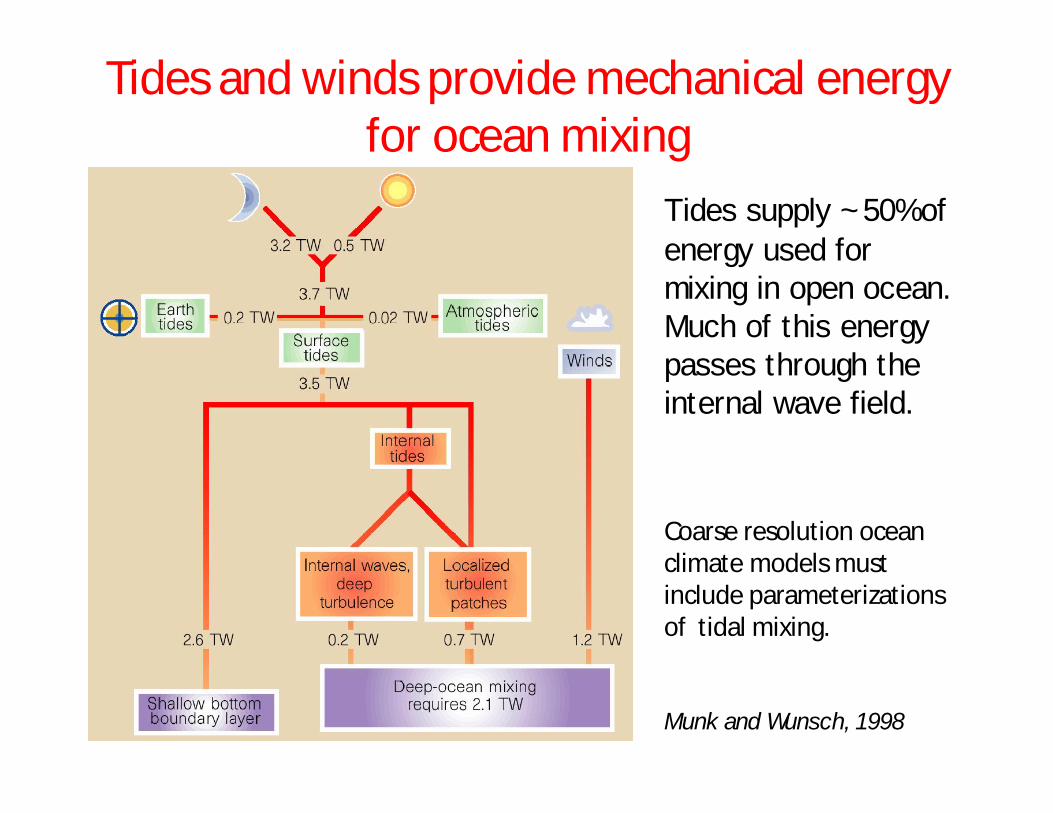
Munk and Wunsch, 1998

Tides supply ~50% of energy used for mixing in open ocean. Much of this energy passes through the internal wave field.

Tides and winds provide mechanical energy for ocean mixing

Coarse resolution ocean climate models must include parameterizations of tidal mixing.

Internal wave driven mixing pathways

MacKinnon et al, 2017, BAMS

Internal wave driven mixing Climate Process Team

Winds, tides and subinertial flow generate internal waves, which propagate, and eventually break. Some of the wave energy leads to mixing across density surfaces (diapycnalmixing), both near and far from the wave generation site.

An energetically consistent framework for parameterizing tidal mixing

Local dissipation

Rate of energy conversion from barotropic tide to baroclinic per unit area.

Vertical structure function∫ 퐹 푧 푑푧 = 1

Fraction of local dissipation.Set (arbitrarily) to 1/3 in current implementations

)(),(1 zFqyxE

St Laurent et al, 2002

2N

Mixing efficiency

Local and remote dissipation: globally require ∫ 휀푑푉 = ∫퐸 푥, 푦 푑푥푑푦

Exponential decay with (arbitrary) constant vertical scale in current implementations

(Osborn, 1980)

Break down the components of this parameterization and its improvements

• Tracer diffusivity expressed in terms of turbulent kinetic energy dissipation (Osborn, 1980): 휅 = 휀

• Energy conversion from barotropic to baroclinic tides: 퐸(푥, 푦)

• Local breaking of internal tides: 푞,퐹(푧)• Farfield breaking of internal tides: (1 − 푞)• Toward a global parameterization: 휅(푥,푦, 푧, 푡)• Impact of tidally-driven mixing parameterizations on ocean

circulation and climate

)(),(1 zFqyxE

2N

Outline

Tracer diffusivity from turbulent kinetic energy budget (Osborn, 1980)TKE eqn: 휕

휕푡 + 푢휕휕푥

푢2 =

휕휕푥 퐹 , − 휖 + 푃 + 퐵

퐹 , = −1휌 푢 푝 훿 , + 휈

휕휕푥

푢2 − 푢 푢 푢

B = 푏 푤′

휖 = 휈휕푢휕푥

푃 = −푢 푢휕휕푥 푢

Transport

Dissipation

Shear production Buoyant production

퐵 = 푏 푤 = −휅 = −휅 푁 where 휅 is the eddy diffusivity of buoyancy.

For steady state, closed volume: 휖 = 푃 + 퐵Define flux Richardson number 푅 = −

휅 = ( )

= Γ where Γ = mixing efficiency.

For stratified turbulence, Γ ≈ 0.2 (subject of active research, see Chris Howland’s poster).

Energy conversion from barotropic to baroclinic tide: Governing parameters for tidal flow over topography

Topography: height h, width L, depth HFlow: speed U, oscillation frequency w

Nondimensional parameters

Topography

Flow

sh

2/1

22

22

ωω

N

fmks

Others: coriolis f, buoyancy frequency N

Hh

ωLURL Nh

UFr

Wave slope

Relative steepness

Relative height

Tidal excursion

Froude numbers

pw C

UFr

H

Lh

Garrett and Kunze, 2007

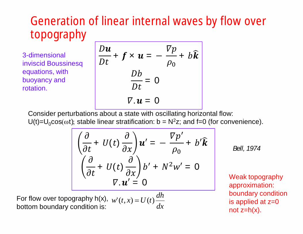
Generation of linear internal waves by flow over topography

Consider perturbations about a state with oscillating horizontal flow: U(t)=U0cos(wt); stable linear stratification: b = N2z; and f=0 (for convenience).

3-dimensional inviscid Boussinesq equations, with buoyancy and rotation.

For flow over topography h(x), bottom boundary condition is: dx

dhtUxtw )(),('

Weak topography approximation: boundary condition is applied at z=0 not z=h(x).

퐷풖퐷푡

+ 풇 × 풖 = − 훻푝휌

+ 푏풌

훻.풖′ = 0

휕휕푡

+ 푈(푡)휕휕푥

풖′ = − 훻푝휌

+ 푏′풌

휕휕푡

+ 푈(푡)휕휕푥

푏 + 푁 푤′ = 0

훻.풖 = 0

퐷푏퐷푡

= 0

Bell, 1974

Internal tide generation schematic

Z=0

h=h0sin(kx)

U0cos(wt)

W=U(t)dh/dx

Sinusoidal topography

Acoustic limit

If 1')cos(' 00

kU

xutU

tu

Then we can simplify equations:

0'' 2222

2

wNwt H

Wave equation:

)cos()cos()0( 00 kxktUhzw

훻.풖′ = 0

휕휕푡풖′ = −

훻푝휌

+ 푏′풌

휕휕푡푏 + 푁 푤′ = 0

Acoustic limit solutions

Satisfies boundary conditions, and has upward group velocity

))(exp())(exp(Re21

00 tmzkxitmzkxikhUw

2

2222 )(

NkmU0 =0.2m/s,

lx=10/3km, N=2e-3/s.

W (m/s), snapshot

Leftward propagating wave Rightward propagating wave

Cg

Cg

Cg

CpCp

Cp

Net wave

( ( 20

20

2/12222104

1 hkUfNE f Acoustic limit energy flux <w’p’>:

Full linear internal tide solution (Bell (1974) solution)

( ( 20

0212/1

1

2222220 hkUJkfnnNnE n

n

nf

N

Nn

nn tnmzkitnmzkihkUJnw

10

0 ))(exp())(exp(Re21

( ( 20

20

2/12222104

1 hkUfNE f

nkUkUJn

n

200

)sin(0 tUx

nJ Bessel function of order n

For small kU/w

Solution consists of fundamental frequency w and higher harmonics nw

So if kU/w<<1, then fundamental dominates and

where nN is the largest integer < N/w

≈ 푁푘푈 ℎfor 푁 ≫ 휔 ≫ 푓

Egbert and Ray, 2000

Energy loss from M2 tide, deduced from Topex-Poseidon SST: frictional dissipation in shallow seas, conversion to baroclinictide in deep ocean.

Jayne and St Laurent, 2001

2202

1),( ukhNyxE b

Energy conversion from barotropic to baroclinictide, from parameterization.

Barotropic to baroclinic energy conversion: comparison with observations

Extensions to energy conversion theoretical predictions

Generalize linear theory for arbitrary topographic shape and finite ocean depth H

( (

1

0222/1

1

2222220

|)(ˆ|2 0

j

jnn

jnn

nf

kUJ

jkh

fnnNndxEP

2/1

222

222

nNfn

Hjk jn

Resonant wavenumbers)(ˆ jnkh =fourier transform topography

Khatiwala (2003), Llewellyn Smith and Young (2002)

Steep topography: 훾 ≥ 1Relaxing linearization of bottom boundary condition (but retaining linearized NS eqns)(Balmforth and Peacock, 2009)

훾

Normalized energy flux

Suppressed energy conversion for steep topography included in global parameterization of tidal mixing at small-scale abyssal hills by Melet et al, 2013.

Examples of solutions in linear regime

2

20

0 2)(exp

Lxxhh

h0=200m, L=10,000mH=4700m,w=1.41s-1

U0=2cm/s

U0=24cm/s

Baroclinic horizontal velocity snapshots

Vertical velocity power spectrum

For U0/(wL)<<1, spectrum is dominated by forcing frequency

Simulations with MITgcm, Legg and Huijts, 2006

Examples of solutions with 훾 > 1, increasing RL=U/(L w ): Generation of higher harmonics

Baroclinic velocity snapshots for low, narrow topography (Legg and Huijts, 2006)

U0=8cm/s U0=16cm/sMore beams, at steeper angles, corresponding to 2w, 3w, 4w appear as U0 increases.

Actual power spectra

Theoretical power spectra

Linear theory (Bell, 1975) predicts higher harmonics well

RL = 1.4 RL = 2.8

U0=2cm/s

RL = 0.35

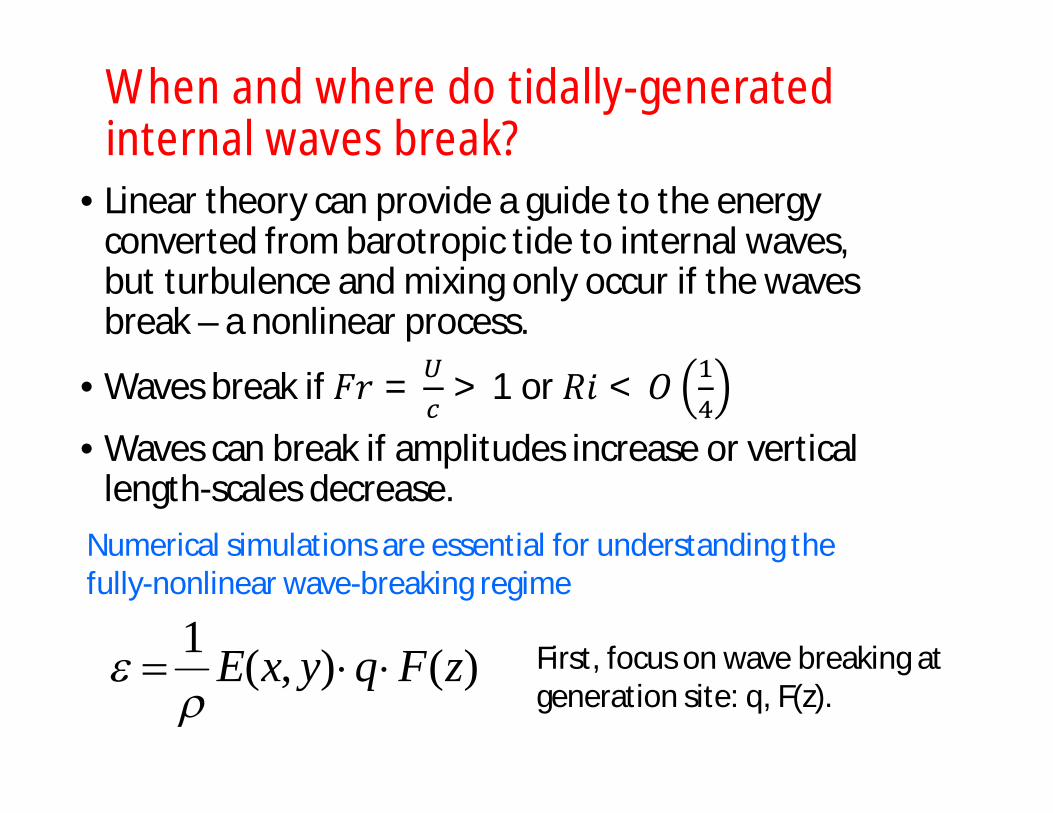
When and where do tidally-generated internal waves break?

• Linear theory can provide a guide to the energy converted from barotropic tide to internal waves, but turbulence and mixing only occur if the waves break – a nonlinear process.

• Waves break if 퐹푟 = > 1 or 푅푖 < 푂• Waves can break if amplitudes increase or vertical

length-scales decrease. Numerical simulations are essential for understanding the fully-nonlinear wave-breaking regime

)(),(1 zFqyxE

First, focus on wave breaking at generation site: q, F(z).

Local dissipation at small amplitude rough topography

2N

Diffusivity inferred from microstructure observations (Brazil Basin)

(Polzin et al, 1997)Comparison between observed and simulated dissipation for tidal flow over rough topography (Nikurashin and Legg, 2011).

What is responsible for mixing well above bottom boundary?

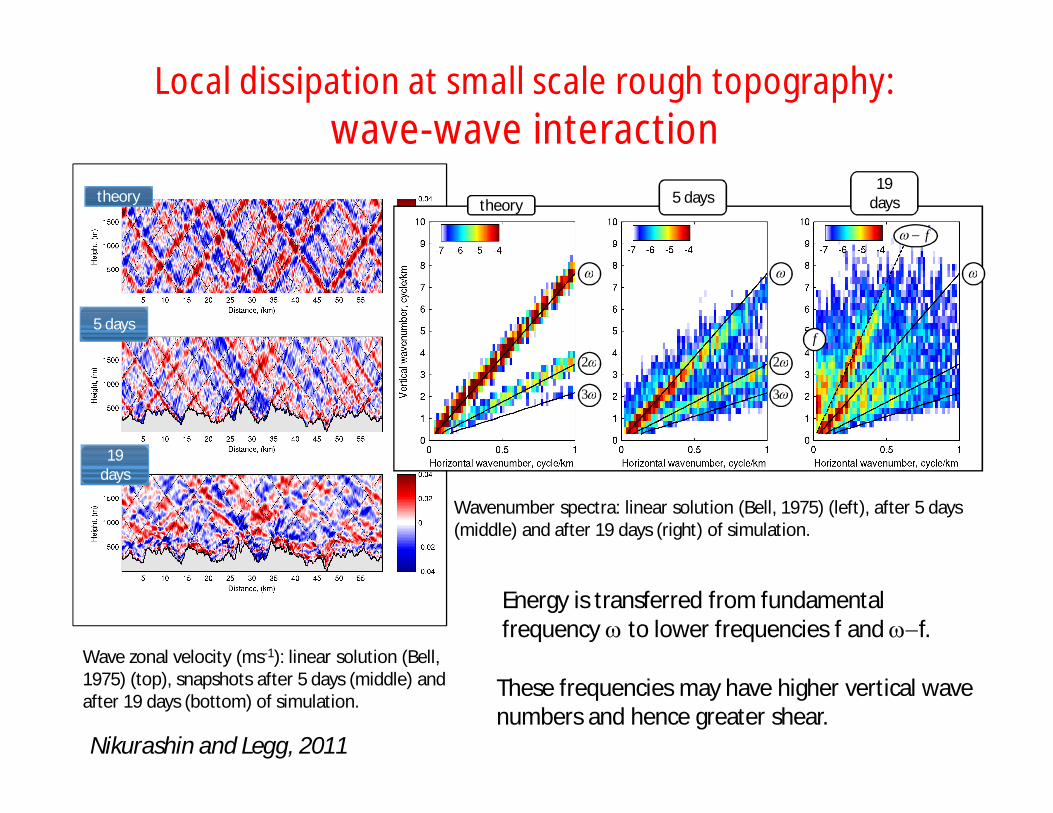
Wave zonal velocity (ms-1): linear solution (Bell, 1975) (top), snapshots after 5 days (middle) and after 19 days (bottom) of simulation.

theory

5 days

19 days

theory 5 days19

days

2

3

f

f

2

3

Wavenumber spectra: linear solution (Bell, 1975) (left), after 5 days (middle) and after 19 days (right) of simulation.

Local dissipation at small scale rough topography: wave-wave interaction

Energy is transferred from fundamental frequency w to lower frequencies f and wf.

These frequencies may have higher vertical wave numbers and hence greater shear.

Nikurashin and Legg, 2011

Local dissipation at small-scale rough topography:Dissipation is enhanced by wave-wave interactions

(Yi, Legg and Nazarian, 2017)

(a) (b)Dissipation profile is sensitive to Coriolis and topographic wavelength (constant forcing and topographic height)

Fixed topographic wavelength (휆 =12km)

Fixed Coriolis (f=7 × 10 푠 = 휔/2)

Horizontally and temporally averaged dissipation

Enhanced dissipation at critical latitude (f = w/2)

Non-monotonic dependence on wavelength

Local dissipation at small-scale rough topography:Wave-wave interaction regimes depend

non-monotonically on topographic steepness

Subcritical slope

Critical slope

Supercritical slope

No rotation 푓 = 휔/2

No enhancement of dissipation at critical latitude when 훾 = 1.71

훾 = 훻ℎ/푠=relative steepness

푠 = = wave steepness

Wave-wave interactions reduce Richardson number at critical latitude

Little increase in low Richardson number region for g1.71

Local dissipation at small-scale rough topography: Wave-wave interaction regimes depend on topographic steepness

Subcritical topography: dissipation decreases with increasing wavelength, peaks around critical latitude.

Supercritical topography: little dependence of dissipation on wavelength or Coriolis.

푞 =

=fraction of energy dissipated locally

At subcritical topography, resonant triad interactions at critical latitude lead to enhanced dissipation.

Local dissipation: internal wave breaking near a tall steep generation site

Klymak et al, 2008

Observed dissipation at Hawaiian ridge-700m

46km-1760m

Legg and Klymak, 2008

Buoyancy field forced by M2 barotropic tide

Wave breaking occurs in transient internal hydraulic jumps, when 훾 > 1, and topography is large: ⁄ > 1

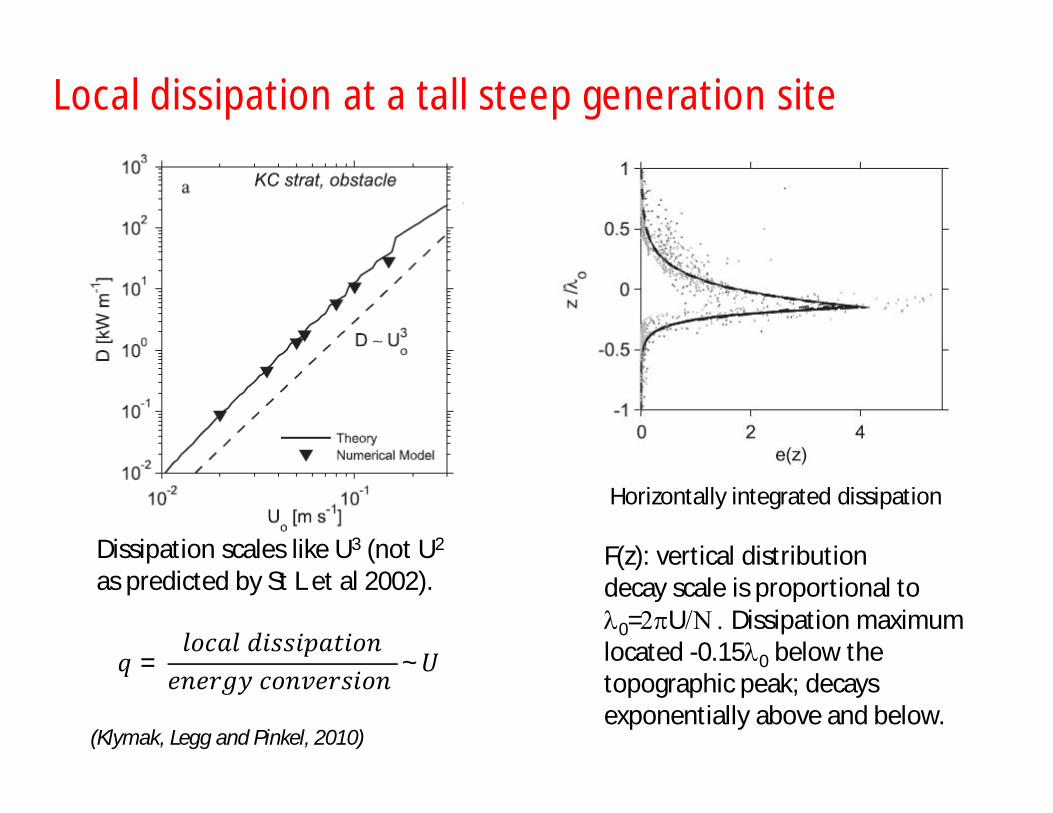
Local dissipation at a tall steep generation site

Dissipation scales like U3 (not U2

as predicted by St L et al 2002).

푞 =푙표푐푎푙 푑푖푠푠푖푝푎푡푖표푛푒푛푒푟푔푦 푐표푛푣푒푟푠푖표푛

~푈

(Klymak, Legg and Pinkel, 2010)

Horizontally integrated dissipation

F(z): vertical distribution decay scale is proportional to l0=2pU/N . Dissipation maximum located -0.15l0 below the topographic peak; decays exponentially above and below.

2D simulations at west ridge : transient arrested waves

Buijsman et al, 2012, 2013

Local dissipation at tall steep topography: Interaction between neighboring ridges

What happens to propagating low modes?

Low modes radiate away, possibly eventually scattering from distant topography

Klymak et al, 2012

Even at Luzon Straits 푞 =

< 50%

Most internal wave energy propagates away from generation site

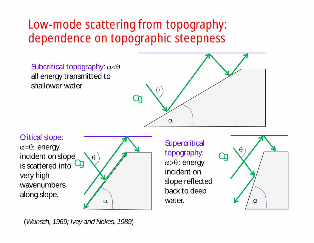
Low-mode scattering from topography: dependence on topographic steepness

q

a

Cgq

a

Cg

q

a

Cg

Subcritical topography: aqall energy transmitted to shallower water

Critical slope: aq: energy incident on slope is scattered into very high wavenumbers along slope.

Supercritical topography: aq: energy incident on slope reflected back to deep water.

(Wunsch, 1969; Ivey and Nokes, 1989)

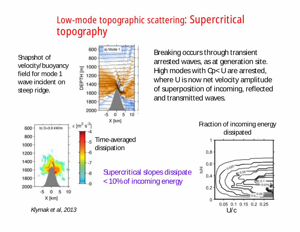
Low-mode topographic scattering: Supercritical topography

Breaking occurs through transient arrested waves, as at generation site. High modes with Cp< U are arrested, where U is now net velocity amplitude of superposition of incoming, reflected and transmitted waves.

Klymak et al, 2013

Snapshot of velocity/buoyancy field for mode 1 wave incident on steep ridge.

Time-averaged dissipation

Fraction of incoming energy dissipated

U/c

Supercritical slopes dissipate < 10% of incoming energy

Low-mode topographic scatteringNear-critical topography

q

a

Cg

Critical slope: aq: energy incident on slope is scattered into very high wavenumbers along slope.

Dissipation increases approximately linearly with h/H.

Time-averaged dissipation, scaled by U2/T (log10 scale)

Up to 100% of incoming energy is dissipated along the slope, independent of wave amplitude.

Fraction of incoming energy

dissipated

h/H Legg, 2014

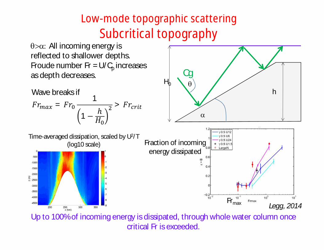
qa: All incoming energy is reflected to shallower depths. Froude number Fr = U/Cp increases as depth decreases.

퐹푟 = 퐹푟1

1 − ℎ퐻

> 퐹푟

Legg, 2014

Low-mode topographic scatteringSubcritical topography

Wave breaks if

Time-averaged dissipation, scaled by U2/T (log10 scale)

Up to 100% of incoming energy is dissipated, through whole water column once critical Fr is exceeded.

Fraction of incoming energy dissipated

Frmax

q

a

CgH0

h

Legg, 2014

BasinsDepth >500m

Wave-wave interactions

Does it matter where tidally-driven ocean mixing happens?

)()(1 zF

AreatE

qr

globalrr

Remote dissipation parameterization:

Climate model thought experiment: examine impact of different idealized horizontal distributions of remote dissipation, dividing ocean into 3 zones

SlopesSlope > 0.01.

Wave reflection/scattering

Continental shelvesWave shoaling

Assign constant value of qr for each zone

• GFDL ESM2G 1000-year simulations with 1860 forcing include St Laurent et al (2002) representation of local tidal dissipation, with 20% dissipated locally.

• Remaining 80% dissipated in 1 of 3 zones. • Reference experiment: 20% local, 80% dissipated via uniform 휅 = 1.4 × 10 푚 푠

Melet et al, 2016

Influence of horizontal location of mixing on Atlantic Meridional Overturning Circulation

Reference: 20% local, 80% uniform diffusivity

20% local, 80% coasts 20% local, 80% basins 20% local, 80% slopes

Atlantic MOC (Sv)

∆AMOC (Sv)

• Mixing on shelves/straits weakens AMOC

• Deep mixing strengthens/deepens AMOC

Melet et al, 2016

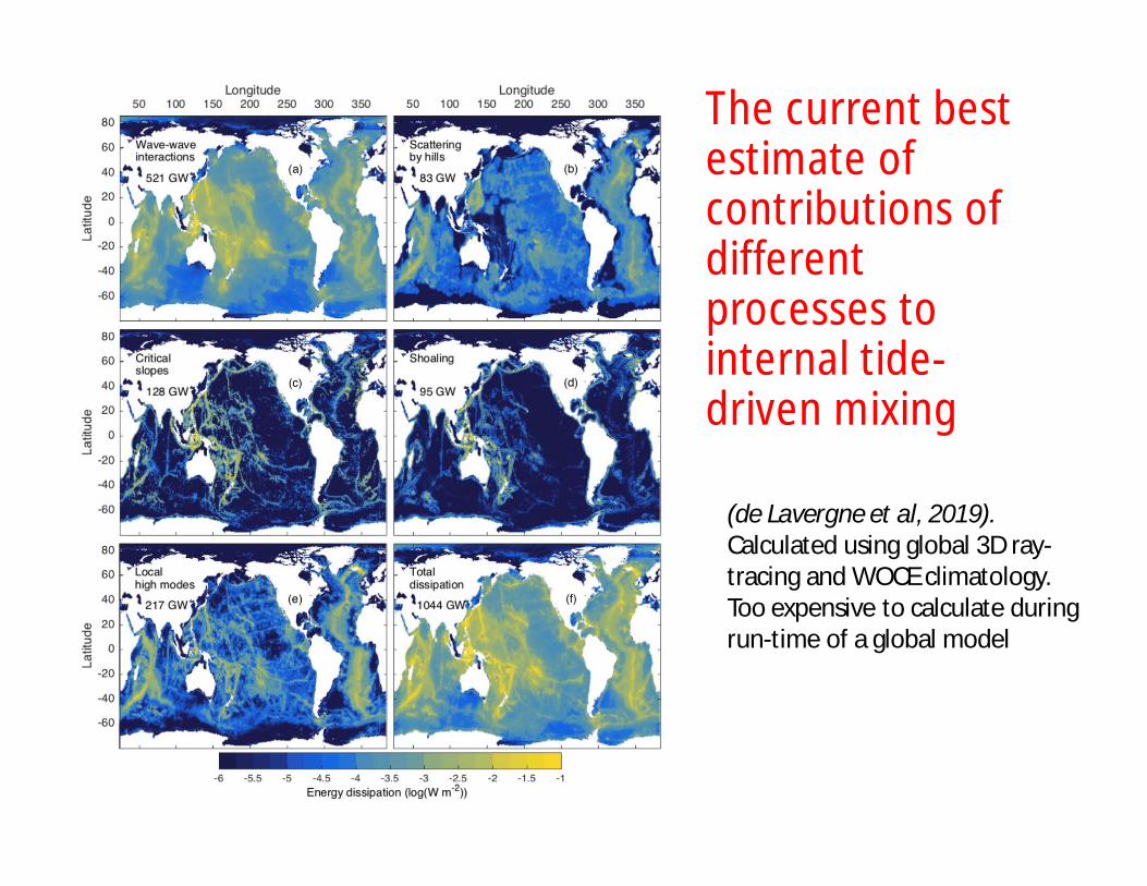
The current best estimate of contributions of different processes to internal tide-driven mixing

(de Lavergne et al, 2019). Calculated using global 3D ray-tracing and WOCE climatology. Too expensive to calculate during run-time of a global model

Theoretical tidally-generated dissipation compares reasonably well with observational fine-structure estimates of dissipation

de Lavergneet al, 2019

Kunze 2017

Summary• Representation of tracer diffusivity in terms of turbulent kinetic

energy dissipation- 휅 = 휀 : allows formulation of an energetically consistent global parameterization

• Energy conversion from barotropic to baroclinic tides: 퐸(푥,푦): depends on topographic amplitude and shape, tidal flow, stratification

• Local breaking of internal tides: 푞,퐹(푧): influenced by PSI, transient hydraulic jumps, topographic height and steepness, latitude

• Farfield breaking of internal tides: (1 − 푞): topographic scattering from continental slope topography

• Toward a global parameterization: 휅(푥,푦, 푧, 푡): must account for all of the above and more: generation, local breaking, propagation, farfield breaking.

• Impact of tidally-driven mixing parameterizations on ocean circulation and climate: Spatial distribution of tidally-driven mixing can lead to 10-25% changes in AMOC

)(),(1 zFqyxE