Thèse de doctorat de l'Université Paris-Saclay …...M. Alain Ayong Le Kama Professeur Directeur...
154
◦ 581
Transcript of Thèse de doctorat de l'Université Paris-Saclay …...M. Alain Ayong Le Kama Professeur Directeur...
NNT : 2016SACLA012
1
Thèse de doctorat
de l'Université Paris-Saclay
préparée à AgroParisTech
Ecole doctorale n◦581Agriculture, alimentation, biologie, environnement et santé
(ABIES)
Spécialité de doctorat : Sciences économiques
par
M. Nicolas Legrand
Revisiting the competitive storage model as a tool for
the empirical analysis of commodity price volatility
Thèse présentée et soutenue à Paris, le 21 novembre 2016.
Composition du Jury :
M. Alain Ayong Le Kama Professeur Directeur de thèse
Université Paris-Ouest Nanterre
M. Brian D. Wright Professeur Rapporteur
Université de Californie, Berkeley
M. Jean-Christophe Bureau Professeur Examinateur
AgroParisTech
M. John P. Rust Professeur Examinateur
Université de Georgetown, Washington DC
M. Nour Meddahi Professeur Rapporteur
Université de Toulouse 1 Capitole
M. Stéphane De Cara Directeur de recherche Co-directeur de thèse
INRA
Mme Valérie Mignon Professeure Présidente
Université Paris-Ouest Nanterre

Titre : Reconsidérer le modèle de stockage compétitif comme outil d'analyse empi-
rique de la volatilité des prix des matières premières
Keywords : Inference Bayésienne, estimation structurelle, volatilité des marchés des matièrespremières, stockage, tendances, investissement
Résumé : Cette thèse propose une analyse empirique et théorique de la volatilité des prixdes matières premières en utilisant le modèle de stockage compétitif à anticipations rationnelles.En substance, la théorie du stockage stipule que les prix des commodités sont susceptibles des'envoler dès lors que les niveaux de stocks sont bas et donc dans l'incapacité de prémunir lemarché contre des chocs exogènes. L'objectif principal poursuivit dans ce travail de recherche estd'utiliser les outils statistiques pour confronter le modèle de stockage aux données a�n d'évaluerle bien-fondé empirique de la théorie du stockage, identi�er ses potentiels défauts et proposerdes solutions possibles a�n d'améliorer son pouvoir explicatif. Dans ce contexte, la diversité desapproches économétriques employées jusqu'à présent pour tester le modèle et ses prédictionsthéoriques est passée en revue dans le chapitre introductif (Ch. 2). Dans l'ensemble, malgré soncaractère relativement parcimonieux, le modèle de stockage s'avère être en mesure de repro-duire de nombreux faits stylisés observés dans les données de prix. Cela étant, il existe toujoursdes caractéristiques des prix non expliquées, comme les hauts niveaux d'autocorrélations ou lesco-variations excessives. Les chapitres suivants explorent trois pistes di�érentes pour essayerd'augmenter la cohérence empirique du modèle de stockage. Le chapitre 3 repose sur l'idée qu'ilexiste des mouvements de long-termes dans les prix des matières premières qui n'ont rien à voiravec la théorie du stockage. Ceci tend à être con�rmé par les résultats obtenus par la mise enoeuvre d'une méthode d'estimation hybride permettant de déterminer conjointement les para-mètres fondamentaux du modèle avec ceux caractérisant la tendance. En e�et, les estimationsdes paramètres structurels sont plus plausibles et le modèle s'ajuste mieux aux données. Dansle chapitre 4, la procédure de test de la théorie du stockage est encore approfondie grâce audéveloppement d'une méthode empirique pour estimer le modèle à la fois sur données de prix etde quantités, une première dans la littérature. L'apport d'information supplémentaire permetd'estimer et de comparer des spéci�cations alternatives et plus riches du modèle, d'inférer desparamètres tels que les élasticités d'o�re et de demande, qui ne sont pas identi�ables lorsqueseuls les prix sont utilisés pour l'estimation. Une autre nouveauté est que des méthodes Bayé-siennes sont utilisées pour l'inférence au lieu des approches fréquentistes employées jusqu'àprésent. Ces deux innovations devraient permettre d'ouvrir la voie à des recherches futures enpermettant l'estimation de modèles aux structures plus complexes. Le dernier chapitre est plusthéorique et porte sur l'extension du volet o�re du modèle en prenant en compte la dynamiqued'accumulation du capital. Sur le plan conceptuel, le stockage n'est autre qu'une seconde formed'investissement, et par conséquent les deux variables d'investissement et de stockage devraientjouer des rôles primordiaux dans la dynamique des prix spot et futures sur les marchés mon-diaux des commodités. Cette intuition est con�rmée par les résultats des simulations obtenuesavec un modèle de stockage augmenté de l'investissement, qui sont assez bien en adéquationavec les données du pétrole brut. Le résultat principal est l'e�et d'éviction qu'a le stockage surl'investissement.
Université Paris-Saclay
Espace Technologique / Immeuble Discovery
Route de l'Orme aux Merisiers RD 128 / 91190 Saint-Aubin, France
3
Title : Revisiting the competitive storage model as a tool for the empirical analysis
of commodity price volatility
Keywords : Bayesian inference, non-linear dynamic models, structural estimation, commo-dity markets volatility, trends, storage, investment.
Abstract : This thesis proposes an empirical and theoretical analysis of commodity price vola-tility using the competitive storage model with rational expectations. In essence, the underlyingstorage theory states that commodity prices are likely to spike when inventory levels are lowand cannot bu�er the market from exogenous shocks. The prime objective pursued in this dis-sertation is to use statistical tools to confront the storage model with the data in an attemptto gauge the empirical merit of the storage theory, identify its potential �aws and provide pos-sible remedies for improving its explanatory power. In this respect, the variety of econometricstrategies employed so far to test the model itself or its theoretical predictions are reviewed inthe opening survey (Ch. 2). On the whole, in spite of its relative parsimony, the storage modelproves able to replicate many of the key features observed in the price data. That said, there arestill some important observed price patterns left unexplained, including the high levels of serialcorrelation and the excessive co-movements. The subsequent chapters explore three di�erentroutes with the aim of increasing the empirical relevance of the storage framework. Chapter 3rests on the idea that there might exist long-term movements in the raw commodity price serieswhich have nothing to do with the storage theory. This tends to be con�rmed by the resultsobtained by implementing a hybrid estimation method for recovering jointly the modelâs deepparameters with those characterizing the trend. Indeed, the estimates of the structural para-meters are more plausible and the model �ts the data better. In chapter 4, the testing of thestorage theory is pushed even further thanks to the development of an empirical strategy totake the storage model to the data on both prices and quantities, for the �rst time in the lite-rature. Bringing additional information allows to estimate and compare alternative and richerspeci�cations of the model, and to infer parameters like the supply and demand elasticities,which are left unidenti�ed when using prices alone. Another novelty is that Bayesian methodsare used for inference in contrast to the frequentist approaches employed thus far. Hopefullyboth these innovations should help paving the way for future research in allowing for the esti-mation of more complex model set-ups. The last chapter is more theoretical as it deals with thestorage model extension on the supply side to account for the dynamics of capital accumulation.Conceptually, storage is nothing but another kind of investment, and thus both investment andstorage variables should play prime roles in driving the spot and futures prices dynamics inworld commodity markets. This intuition is con�rmed by the simulation results obtained withthe investment-augmented storage model which are fairly well backed up by the crude oil data.The key �nding is the crowding-out e�ect of storage on investment.
Université Paris-Saclay
Espace Technologique / Immeuble Discovery
Route de l'Orme aux Merisiers RD 128 / 91190 Saint-Aubin, France
4
Contents
Remerciements i
1 Introduction 11.1 Motivation . . . . . . . . . . . . . . . . . . . . . . . . . . . . . . . . . . . . . . . . . . . . 11.2 Empirical strategies in macroeconomics . . . . . . . . . . . . . . . . . . . . . . . . . . . . 2
1.2.1 Two complementary approaches . . . . . . . . . . . . . . . . . . . . . . . . . . . . 21.2.2 One and not the place to start . . . . . . . . . . . . . . . . . . . . . . . . . . . . . . 4
1.3 Organization of the dissertation . . . . . . . . . . . . . . . . . . . . . . . . . . . . . . . . . 5
2 Review and Perspectives 82.1 Two views of commodity price fluctuations . . . . . . . . . . . . . . . . . . . . . . . . . . 102.2 Empirical validation as justice of the peace . . . . . . . . . . . . . . . . . . . . . . . . . . . 10
2.2.1 Confronting the cobweb models to the data . . . . . . . . . . . . . . . . . . . . . . 112.2.2 Empirical performance of the competitive storage model . . . . . . . . . . . . . . . 122.2.3 The excess co-movement puzzle . . . . . . . . . . . . . . . . . . . . . . . . . . . . 26
2.3 The interest rate channel . . . . . . . . . . . . . . . . . . . . . . . . . . . . . . . . . . . . 282.3.1 The latent Hotelling’s rule . . . . . . . . . . . . . . . . . . . . . . . . . . . . . . . 292.3.2 The exchange rate pass-through . . . . . . . . . . . . . . . . . . . . . . . . . . . . 302.3.3 The overshooting theory . . . . . . . . . . . . . . . . . . . . . . . . . . . . . . . . 33
2.4 The outlook . . . . . . . . . . . . . . . . . . . . . . . . . . . . . . . . . . . . . . . . . . . 35
3 Trending Commodity Prices 373.1 The model . . . . . . . . . . . . . . . . . . . . . . . . . . . . . . . . . . . . . . . . . . . . 40
3.1.1 Model equations . . . . . . . . . . . . . . . . . . . . . . . . . . . . . . . . . . . . 403.1.2 How can storage generate high serial correlation? . . . . . . . . . . . . . . . . . . . 42
3.2 Econometric procedure . . . . . . . . . . . . . . . . . . . . . . . . . . . . . . . . . . . . . 433.2.1 Trend specifications . . . . . . . . . . . . . . . . . . . . . . . . . . . . . . . . . . 443.2.2 The likelihood estimator . . . . . . . . . . . . . . . . . . . . . . . . . . . . . . . . 45
3.3 Estimation results . . . . . . . . . . . . . . . . . . . . . . . . . . . . . . . . . . . . . . . . 483.3.1 Data . . . . . . . . . . . . . . . . . . . . . . . . . . . . . . . . . . . . . . . . . . . 483.3.2 Model selection . . . . . . . . . . . . . . . . . . . . . . . . . . . . . . . . . . . . . 483.3.3 No trend . . . . . . . . . . . . . . . . . . . . . . . . . . . . . . . . . . . . . . . . 493.3.4 Models with a time trend . . . . . . . . . . . . . . . . . . . . . . . . . . . . . . . . 543.3.5 Model predictions . . . . . . . . . . . . . . . . . . . . . . . . . . . . . . . . . . . 55
3.4 Conclusion . . . . . . . . . . . . . . . . . . . . . . . . . . . . . . . . . . . . . . . . . . . 583.A Numerical method . . . . . . . . . . . . . . . . . . . . . . . . . . . . . . . . . . . . . . . 603.B Computational details . . . . . . . . . . . . . . . . . . . . . . . . . . . . . . . . . . . . . . 60

6 CONTENTS
3.C Small sample properties . . . . . . . . . . . . . . . . . . . . . . . . . . . . . . . . . . . . . 613.D Supplementary tables . . . . . . . . . . . . . . . . . . . . . . . . . . . . . . . . . . . . . . 643.E Supplementary figures . . . . . . . . . . . . . . . . . . . . . . . . . . . . . . . . . . . . . 67
4 Bayesian Estimation of the Storage Model using Information on Quantities 684.1 The Model . . . . . . . . . . . . . . . . . . . . . . . . . . . . . . . . . . . . . . . . . . . . 69
4.1.1 Model equations . . . . . . . . . . . . . . . . . . . . . . . . . . . . . . . . . . . . 694.1.2 Model solution . . . . . . . . . . . . . . . . . . . . . . . . . . . . . . . . . . . . . 72
4.2 Overview of the grains market . . . . . . . . . . . . . . . . . . . . . . . . . . . . . . . . . 734.2.1 Data . . . . . . . . . . . . . . . . . . . . . . . . . . . . . . . . . . . . . . . . . . . 734.2.2 Descriptive statistics . . . . . . . . . . . . . . . . . . . . . . . . . . . . . . . . . . 75
4.3 Estimation . . . . . . . . . . . . . . . . . . . . . . . . . . . . . . . . . . . . . . . . . . . . 774.3.1 The likelihood function . . . . . . . . . . . . . . . . . . . . . . . . . . . . . . . . . 784.3.2 Prior distribution of the parameters . . . . . . . . . . . . . . . . . . . . . . . . . . 814.3.3 Posterior estimates of the parameters . . . . . . . . . . . . . . . . . . . . . . . . . 82
4.4 Conclusion . . . . . . . . . . . . . . . . . . . . . . . . . . . . . . . . . . . . . . . . . . . 86
5 The Crowding-Out Effect of Storage on Investment 895.1 Preamble . . . . . . . . . . . . . . . . . . . . . . . . . . . . . . . . . . . . . . . . . . . . 905.2 Introduction . . . . . . . . . . . . . . . . . . . . . . . . . . . . . . . . . . . . . . . . . . . 975.3 Complementary theories: A Literature Review . . . . . . . . . . . . . . . . . . . . . . . . . 99
5.3.1 Investment dynamics and constraints . . . . . . . . . . . . . . . . . . . . . . . . . . 995.3.2 The competitive storage model . . . . . . . . . . . . . . . . . . . . . . . . . . . . . 1005.3.3 The determinants of futures pricing . . . . . . . . . . . . . . . . . . . . . . . . . . 102
5.4 Theory and Facts . . . . . . . . . . . . . . . . . . . . . . . . . . . . . . . . . . . . . . . . 1055.4.1 A tale of investment and storage . . . . . . . . . . . . . . . . . . . . . . . . . . . . 1055.4.2 The data . . . . . . . . . . . . . . . . . . . . . . . . . . . . . . . . . . . . . . . . . 1065.4.3 Empirical features . . . . . . . . . . . . . . . . . . . . . . . . . . . . . . . . . . . 108
5.5 Model . . . . . . . . . . . . . . . . . . . . . . . . . . . . . . . . . . . . . . . . . . . . . . 1145.5.1 Model’s equations . . . . . . . . . . . . . . . . . . . . . . . . . . . . . . . . . . . 1145.5.2 The competitive equilibrium . . . . . . . . . . . . . . . . . . . . . . . . . . . . . . 1155.5.3 Numerical Solution . . . . . . . . . . . . . . . . . . . . . . . . . . . . . . . . . . . 116
5.6 Simulation Results . . . . . . . . . . . . . . . . . . . . . . . . . . . . . . . . . . . . . . . 1175.6.1 Calibration . . . . . . . . . . . . . . . . . . . . . . . . . . . . . . . . . . . . . . . 1175.6.2 Theoretical insights . . . . . . . . . . . . . . . . . . . . . . . . . . . . . . . . . . . 1185.6.3 Discussion . . . . . . . . . . . . . . . . . . . . . . . . . . . . . . . . . . . . . . . 126
5.7 Conclusion . . . . . . . . . . . . . . . . . . . . . . . . . . . . . . . . . . . . . . . . . . . 132
6 Conclusion 1346.1 General Conclusion . . . . . . . . . . . . . . . . . . . . . . . . . . . . . . . . . . . . . . . 1346.2 Perspectives . . . . . . . . . . . . . . . . . . . . . . . . . . . . . . . . . . . . . . . . . . . 136
Bibliography 146

REMERCIEMENTS
Je commencerai par adresser mes remerciements à mes directeurs de thèses bien sûr, Alain Ayong Le Kama
et Stéphane De Cara, mais aussi à l’ensemble des membres de mon jury de thèse, Mme Valérie Mignon, M.
Jean-Christophe Bureau, M. Nour Meddahi, M. Brian D. Wright et M. John P. Rust pour le temps consacré à
évaluer la qualité scientifique de mes travaux, pour votre aide et vos conseils au combien précieux. Merci
également d’avoir accepté de venir parfois de très loin afin d’assister physiquement à la soutenance.
Pour ce qui est de la vie quotidienne, je tiens à remercier mes camarades de bureau pour avoir supporté
mes envies d’aérer la pièce même brièvement l’hiver, de laisser la porte ouverte y compris quand Mme vient
faire ses photocopies, mes penchants bobos-écolos qui expliquent mon aversion pour le ventilateur l’été,
pour le radiateur électrique qui oblige à utiliser des moufles l’hiver, ou qui me poussent enfin à n’allumer la
lumière que lorsqu’on n’aperçoit plus son clavier. Merci donc à vous Anaïs, Cécilia, Simon et Lise. Plus
généralement, je souhaite remercier l’ensemble des membres de mon laboratoire d’accueil, l’UMR Economie
de publique de l’INRA, où règne solidarité, partage et. . . bonne humeur ! Vraiment toutes les conditions sont
réunies pour se sentir à l’aise dès son arrivée et travailler en toute sérénité. Un seul exemple pour illustrer la
singularité des lieux, la disponibilité de chercheurs expérimentés tel que Jean-Marc Bourgeon. Je connais des
institutions où avoir le privilège de demander des conseils à de tels chercheurs requiert l’envoi d’un mail
avec prise de rendez-vous au moins une semaine à l’avance. Avec Jean-Marc, il n’en est rien, il suffit de
frapper à la porte quand elle n’est pas déjà ouverte. Donc merci beaucoup Jean-Marc pour ta disponibilité,
pour m’avoir fait bénéficier de tes éclairages pertinents et bienveillants tout au long de ces trois ans. C’est
tout simplement exceptionnel.
Exceptionnel ce n’est pas moi qui le dit, c’est Assia une doctorante basée à Paris comme moi, qui travaille
sur les prix des matières premières comme moi, avec des modèles non-linéaires stochastiques comme moi,
qui participait à des summer et winter school comme moi et avec qui j’ai collaboré sur le 3e et dernier article
de ma thèse. Alors merci beaucoup Assia pour ton efficacité et ton sérieux, pour ta bonne humeur contagieuse,
et plus généralement pour cette collaboration qui je l’espère sera aussi fructueuse académiquement qu’elle ne
l’a été humainement et intellectuellement. Merci enfin pour m’avoir permis de rencontrer et de bénéficier des
conseils précieux de chercheurs prestigieux. Je pense en particulier à M. Nicolas Coeurdacier et M. Guy
Laroque. Je vous remercie sincèrement messieurs pour tout le temps que vous nous avez consacré à Assia et
moi.
Merci également à l’entreprise Total et à la Chaire Economie du Climat, Philippe Delacote en tête, avec
qui j’ai eu l’opportunité d’effectuer une mission d’expertise en entreprise en complément de mes activités de

ii REMERCIEMENTS
recherche. C’est notamment grâce au soutien financier de Total que j’ai pu voyager et participer à certaines
conférences ou summer school, ce que beaucoup de doctorant(e)s non tout simplement pas la chance de
pouvoir faire faute de disposer de moyens suffisants. Mais au-delà de l’aspect purement financier ce sont
surtout des éclairages pertinents extérieurs, notamment M. Jean-Michel Brusson, Mme Elise Thomaso, M.
Edouard Tallent, de personnes expertes dans le domaine des matières premières et qui sont au combien
importantes à l’heure d’essayer de prendre un peu de recul sur ces travaux, ce qui n’est jamais évident surtout
quand on est doctorant. Au registre des regards extérieurs je tiens à remercier aussi M. Fabien Tripier pour sa
participation aux réunions du comité de suivi de thèse.
Mais trois ans c’est long et il y a une vie en-dehors du laboratoire et des bibliothèques. A cet égard
je tiens à remercier mon colocataire Simon, doctorant en économie lui aussi et avec qui j’ai pu partager
en plus d’un appartement joies, peines, frustrations et doutes. Son travail sur les liaisons dangereuses fera
autorité à n’en pas douter. Merci aussi à ma famille pour son soutien, pour avoir essayé de (faire semblant de)
comprendre ce que faisait « le professeur Tournesol ».
Enfin je voudrais terminer par adresser des remerciements tout particuliers à Christophe Gouel pour son
accompagnement tout au long de ces trois années, ses précieux conseils prodigués à doses homéopathiques
pour ne pas me décourager, et surtout la transmission de sa passion et de sa rigueur. Du mémoire de fin
d’étude et la rédaction du projet de thèse, jusqu’au tiret manquant à l’avant dernière ligne de la bibliographie
de ce présent manuscrit, en passant par l’optimisation du code afin de gagner une bonne semaine de temps de
calculs, il a été là à chaque fois que j’en avais besoin. Enfin, il m’a également vivement conseillé de participer
à certaines summer et winter school, au cours desquelles j’ai non seulement pu progresser techniquement
mais aussi pu commencer à me constituer un réseau international de jeunes chercheur(e)s. Alors Christophe
vraiment MERCI, MERCI et encore MERCI !!

CHAPTER 1
INTRODUCTION
1.1 MOTIVATION
In 2013, at the beginning of my research, the commodity prices experienced one of their episodic crises,
with crude oil prices lying above the US$ 100 a barrel and a price of the ton of corn close to US$ 250. Such
rocketing prices have devastating consequences in terms of food security on the poorest population, especially
the poorest, and can trigger social unrest and riots. Ironically, although today these same two prices are about
twice as low, the situation is no less worrisome for the government of exporting countries, where national
income primarily relies on the production of one particular basic product. The current social and political
instabilities in Venezuela exemplify the adverse consequences of the recent collapse of the crude oil price.
Actually, whether too high or two low, at both the micro or macro levels, commodity prices affect a large
spectrum of domestic as well as international economic activities, and thus the issues related to their volatility
have always been high on the political agenda.
That said, to take any effective actions, whether designed to smooth the prices fluctuations or to protect
itself against them, there is a need to know what are the main causes of these typical instabilities in commodity
markets. Among the reasons advanced were the rising demand from emerging economies such as China and
India, the biofuels mandates entering in competition with food products, the side-effects of climate change
with more frequent droughts and flooding threatening the global supply, the weaker US dollar in response to
the monetary policy in the US following the 2008 financial crisis or else the financialization of commodity
markets with investors willing to diversify their portfolio and speculating in the financial markets. But there
are many others and nearly each explanation call for a specific remedy, if any, not always compatible with
one another. Worse still, I had the feeling that the difference of opinions varied with the study’s sponsors or
the targeted audience, and reflected more personal beliefs dictated by self-economic interests and political
biases, rather than true objective arguments grounded in “neutral” science. In fairness to these conflicting
views, none of them is completely wrong nor the whole truth and all deserve a careful examination.
In this respect, not really convinced by the explanation brought so far and, in face of the lack of consensus
around issues where the stakes are yet so high, I decided to undertake research and attempt to modestly add
to our common knowledge of the behavior of commodity prices. With hindsight, I must confess that I better

2 CHAPTER ONE
understand the reasons why it is so complicated to draw decisive conclusions about the main factors driving
the world prices dynamics. Nonetheless, this is not to say that nothing can be done for attempting to improve
our understanding of the workings of international markets of basic goods. Given my scientific education, I
naturally chose to tackle the topic on a quantitative front which usually involves statistical techniques. Unlike
the qualitative approaches, any empirical analyses cannot but rely on a model designed to represent and
explore the observed data in a disciplined fashion. The competitive storage model pioneered by Gustafson
(1958) is one such analytical device when it comes to study the aggregate fluctuations of storable commodity
prices. At the heart of the framework is the storage theory stipulating that the ability to store primary products
is an essential determinant of the observed price variations. This thesis is dedicated to evaluate and improve
the empirical relevance of the storage theory in confronting the competitive storage model to the observed
data.
Before delving into the details of the inner working of the storage model, first I would like first to evoke
the variety of statistical tools available, of methods used to be developed in empirical macroeconomics to
provide quantitative answers to the essential concerns related to, among others, the determinants of the
economic growth and unemployment, the effects of monetary and fiscal policies, and the way they relate with
one another. This aims at getting the big picture of the lines of economic research followed in the present
work.
1.2 EMPIRICAL STRATEGIES IN MACROECONOMICS
Global commodity prices being nothing but macroeconomic variables, their study rests on the reservoir of
macroeconometrics techniques set up to isolate regularities, to interpret and identify salient patterns in every
sample of observed data, as well as to uncover correlations and even causalities across variables. As most of
the statistical procedures applied thereafter are borrowed from this toolkit, I will depict a brief summary of
the shared traits between all these econometrics methods along with their main strengths and weaknesses.
1.2.1 TWO COMPLEMENTARY APPROACHES
As demonstrated at length in the survey of Labys (2006, Ch. 1) in the case of commodity prices, there
exists a multitude of econometrics techniques for analyzing a times series whether at the short, medium or
long-run frequencies. They can nevertheless be divided into two major categories known as the structural and
“atheoretical” estimations strategies, whether they incorporate restrictions derived from the economic theory.
A GRADIENT OF ECONOMIC THEORY A first way of studying the variations of macroeconomic variables
is to focus on the aggregated relationships. In this spirit, the models takes the form of regression equations in
which endogenous variables gathered on the left-hand side are explained by a set of exogenous variables
appearing on the right-hand side. The links between the variables can possibly be assumed non-linear to
accommodate more complex dynamics, while the relative explanatory power of each variable is eventually
assessed using standard statistical tests of significance. But in the end, the logic is still to “let the data speak”

INTRODUCTION 3
and reveals both the nature and the significance of the relationships as well as dependencies between the
variables of interest. This ad-hoc characterization of the macroeconomic behavior is a quite flexible and
robust way of summarizing the properties of the data. The thing is that the results are hardly interpretable
without a minimum of economic theory. Put crudely, to pass from observed correlations to conclusions about
causality relationships often requires to incorporate some theoretical assumptions.
This is where the alternative structural strategy takes on its full meaning. More precisely, the gist
of the methodology is to combine the data with a set of theoretical restrictions mostly derived from the
microeconomic principles including the specification of production and consumption functions, market
equilibrium conditions (e.g., market clearing, accounting identities), the agents’ behavior, namely the way
dynamic decisions are made. Embedding additional information borrowed from the economic theory should
in principle guarantee the model internal consistency, and enable a clear and hopefully direct economic
interpretation of the values of the estimated parameters. Nonetheless, if the modeling relies on inadequate
assumptions the model’s fit is worse and the whole theoretical structure can well be rejected by the data.
Actually, there is no such thing as a divide between both approaches since there exists a continuum of models
depending on the degree of economic constraints integrated in the estimation procedure. In addition, more
often than not the reduced-form versions of structural models prove useful to assess the relevance of a theory
in formally testing the validity of the restrictions the latter imposed on the data (Deaton and Laroque, 1992).
THE CHANGE OF PARADIGM The aforementioned distinction between the modeling approaches was
insignificant until the end of the 1970’s since, at that time, the empirical macroeconomics mostly relied
on the structural econometric models (SEMs) which consisted in a mixture of both structural and ad-hoc
equations relating aggregated economic variables and estimated independently of one another. Models of this
type in the case of international commodity markets can be found in Labys (1973). However, not only the
SEMs given their large size–e.g., often several tens of equations–were cumbersome and relatively sluggish,
struggling for example to accommodate structural breaks in the economic environment, but above all they
did not survive both the Lucas (1976) and Sims (1980) critiques. The latter, in turn, marked the start of a new
era in macroeconometrics.
The Lucas (1976) critique has to do with the lack of internal consistency resulting from the juxtaposition
of unrelated equations as is the case in the SEMs,and the fact that the reduced-form relationships include
parameters likely to change with the various government policies and thus deliver invalid conditional
forecasts, needed when it comes to compare the macroeconomic impacts of alternative monetary and
fiscal policies. Therefore, according to Lucas a model should only contain structural equations with deep
parameters invariant to the policy regime. Completed with Sargent (1976)’s econometric work on the power
of rational expectations, this call for internal consistency and microfounded models–i.e., derived from the
intertemporal optimizing behavior of agents–gave birth to the Dynamic Stochastic General Equilibrium
models (DSGEs).1 Unlike the SEMs, the DSGEs models are of smaller size, rest on a sound theoretical
1 See Smets and Wouters (2007) for a standard DSGE model in the modern macroeconometrics literature.
4 CHAPTER ONE
basis squared by microeconomic principles and, above all, are now estimated as a whole system of equations
thereby preserving the internal consistency of the structure.
From Sims’ standpoint, the major empirical failure of the SEMs’ approach was twofold: (i) the estimation
equation by equation which does not allow for interrelationships across variables even though, especially
in macroeconomics, the causalities might well be reciprocal, and (ii) regarding the structural equations, the
assumed character exogenous or endogenous of the different variables and, more broadly, the constraints
imposed by the economic theory might well be at odds with the data, thereby crippling the quality of the
model’s predictions. In other words, Sims (1980) places greater emphasis on the external consistency of
the modeling and thus suggests instead a flexible econometric strategy, known as Vector Autoregressive
models (VARs), in which variables are regressed on their own past values along with those of the related
variables embedded in the model. Having said this, estimation of VARs requires identification restrictions
which can either belong to the shocks ordering or to the economic theory then leading to the Structural
Vector Autoregressive models (SVARs). Studying the propagation of an oil price shock and quantifying its
macroeconomic impacts as is done in Kilian (2008), is one illustration of the SVARs models’ use in the
empirical literature of commodity prices.2
In summary, the modern macroeconometrics relies on two streams of strategies, the choice between both
of them resulting from a trade-off between the targeted level of internal and external coherence, interpretability
of the results and model’s fitting performance. That said, as illustrated with the SVARs models, the boundary
between both new generations of models remains porous.
1.2.2 ONE AND NOT THE PLACE TO START
The following dissertation explores the commodity price volatility using the competitive storage model with
rational expectations as an analytical tool. In substance, it is a basic supply and demand dynamic equilibrium
model of the world commodity market in which storage plays a key role. According to the storage theory,
the market demand not only consists in a demand for immediate consumption, but also in a speculative
demand from forward-looking and rational storers buying in expectations of profits despite the carrying costs
incurred. To complete the set of assumptions, the production is subject to random shocks while the market
clears in every period. Specified like this, the core system of equations structuring the storage model is fully
microfounded thereby insuring internal consistency and thus immunity to the Lucas critique. In addition, as
shown in Cafiero et al. (2011b), even in its crudest form, the canonical storage model proves able to replicate
many typical aspects observed in the commodity price series including nonlinearities, autocorrelation, cluster
of volatility and asymmetries in the distribution.
All in all, the rather clear microfoundations combined with the demonstrated satisfying empirical
performances make the competitive storage model with rational expectations a good candidate to start
thinking about global commodity price volatility. What is more, although it is only a partial equilibrium
model of the global commodity markets, the rational expectations storage model shares many features with
2 Refer also to (Kilian, 2009, Inoue and Kilian, 2013, Kilian and Murphy, 2014, Baumeister and Hamilton, 2015) for more aboutthe use of SVARs models in the context of commodity prices.
INTRODUCTION 5
the DSGE models and thus the empirical studies of price instabilities in world commodity markets pursued
in this thesis sit in this branch of the macroeconometrics literature. Recalling that research advances in
empirical macroeconomics have always resulted from the combinations of theories with facts, I will build
upon the existing body of work dedicated to assess the quantitative merits of the storage theory and, taking
the storage model to the real data, attempt to improve its explanatory power while maintaining its internal
consistency.
From this perspective, I will voluntarily omit, or at best only evoke, the purely statistical approaches
essentially based on the VARs models. This is not to say that I think they are useless, quite the contrary in
fact. Indeed, in many respects these theory-free models directly focused on the aggregated relationships
between the macroeconomic variables of interest and which do not bother with the microfoundations’ issues,
prove to be highly complementary to the structural empirical studies to which this thesis conforms. Among
their main appeal are the often better predictive abilities, the demonstrated greater robustness to the almost
inevitable mispecifications and, even more importantly maybe, their suitability to handle in a quantitative
manner the variety of macroeconomic drivers. More precisely, the ad-hoc relationships can (i) shed light to
some empirical flaws in the modeling such as important observed dynamics not yet explained by the model
but which deserved careful considerations, and even (ii) be used as temporary model’s repairs to capture
a particular phenomenon in the data so as to increase the model’s external consistency the time needed to
develop the adequate microfoundations accounting for the phenomenon in question. For all these reasons
these two pillars of macroeconometrics are definitively not substitute and should work hand-in-hand rather
than being opposed as it happens sometimes. In this spirit, the VAR techniques can deliver very valuable
insights for a comprehensive knowledge of the main drivers governing the behavior of commodity prices
and has its entire place in the empirical analyzes of the commodity price volatility along with the related
discussions. Still, they are well beyond the primary scope of this thesis and thus will not be further examined.
1.3 ORGANIZATION OF THE DISSERTATION
This thesis falls in four main chapters. The first one carries on the Cafiero and Wright (2006)’s textbook
chapter and surveys the empirical strategies designed to take the storage model to the data. It ends by setting
the stage of the rest of the dissertation in suggesting avenues of model’s extensions to increase its explanatory
power, some of which are then followed by the three other chapters. Based on the model’s empirical failures
pointed out in the survey, the subsequent two aim at estimating richer storage model specifications likely
to improve the fitting performance of the model. The last one is more theoretical and, taking the example
of the crude oil market, analyzes the implications in terms of price dynamics resulting from the negative
interactions between investment and storage. It includes a short and self-contained preamble, written for a
non-academic audience, which attempts to offer a narrative of the wild swings in crude oil prices, highlighting
the paramount importance of returning to the supply and demand fundamentals when it comes to try to
understand the dynamics of price in the crude oil market. This justifies the modeling approach adopted
thereafter in the rest of the chapter, namely an extension of the storage model on the supply-side.
6 CHAPTER ONE
CHAPTER 2: A REVIEW OF THE EMPIRICAL PERFORMANCE OF THE STORAGE MODEL This chapter
aims at setting the scene of this thesis. It presents both the history and the state-of-the-art of the empirical
approach of the modeling of the world commodity price volatility, in placing the storage model at the heart
of the analysis while outlining the key milestones. Specifically, I try to offer somebody unfamiliar with the
related literature a gist of the modeling issues at stakes from both a retrospective and speculative view point.
I remain focused on the empirical techniques designed to assess the merits of the storage theory without
trying to be exhaustive, and thereby leaving aside the purely statistical approaches, weakly linked to the
storage model and well beyond the scope of the present dissertation. I conclude by suggesting a research
agenda at all times frames for overcoming the current empirical flaws and hopefully improving the storage
model explanatory power. The subsequent three chapters then deal with one of each of the noted pitfalls in
attempting to provide remedies.
CHAPTER 3: ESTIMATING THE STORAGE MODEL WITH TRENDING PRICES The chapter, co-authored
with Christophe Gouel and to be published in the Journal of Applied Econometrics, presents a method to
estimate jointly the parameters of a standard commodity storage model and the parameters characterizing the
trend in commodity prices. Introduced in the DSGE literature by Canova (2014), this procedure allows the
influence of a possible trend to be removed without restricting the model specification, and allows model and
trend selection based on statistical criteria. The trend is modeled deterministically using linear or cubic spline
functions of time. The results show that storage models with trend are always preferred to models without
trend. They yield more plausible estimates of the structural parameters, with storage costs and demand
elasticities that are more consistent with the literature. They imply occasional stockouts, whereas without
trend the estimated models predict no stockouts over the sample period for most commodities. Moreover,
accounting for a trend in the estimation imply price moments closer to those observed in commodity prices.
Our results support the empirical relevance of the speculative storage model, and show that storage model
estimations should not neglect the possibility of long-run price trends.
CHAPTER 4: BAYESIAN ESTIMATION OF THE STORAGE MODEL USING PRICES AND QUANTITIES This
chapter, written in collaboration with Christophe Gouel, presents a new strategy to estimate the rational
expectations storage model. The main innovations are twofold. First, it uses information on prices and
quantities – consumption and production – in contrast to previous approaches which use only prices. This
additional information allows us to estimate a model with elastic supply, and to identify parameters such as
supply and demand elasticities, which are left unidentified when using prices alone. Second, contrary to the
previous chapter, the estimation relies on the Bayesian methods, popularized in the literature on the estimation
of DSGE models, but so far never used to recover the parameter estimates of the storage model. The primary
reason for this choice is that, as is often the case in the estimation of dynamic models, the likelihood is
flat into certain areas and/or exhibit many local maxima. In this context, the classical inference approach
has trouble finding the global maximum of the likelihood and, as shown in chapter 3, usually requires an
initial grid-search routine to locate a candidate maximum along with the cumbersome implementation of
sophisticated algorithms like simulated annealing. It is even more challenging as the number of parameters
INTRODUCTION 7
to be estimated increases, not to mention the computation of the corresponding standard errors or confidence
intervals. As long as inference is relying on prices alone, given the small number of parameters that can be
freely identified (three at the most), maximizing the likelihood function is not that big a deal. But now with
the increase in the dimensionality of the likelihood function (e.g., up to four times), the superiority of the
Bayesian techniques appears even more obvious. The Bayesian inference is finally carried out on a market
representing the caloric aggregate of the four basic staples – maize, rice, soybeans, and wheat – from 1961 to
2006. The results show that to be consistent with the observed volatility of consumption, production, and
price, elasticities have to be in the lower ranges of the elasticities in the literature, a result consistent with
recent instrumental variable estimations on the same sample (Roberts and Schlenker, 2013).
CHAPTER 5: THE CROWDING-OUT EFFECT OF STORAGE ON INVESTMENT This chapter opens with a
short story of the recent collapse of the most scrutinized crude oil price. Although self-contained and written
in a non-technical fashion, it lays out the main features a model should encapsulate to be able to deliver
consistent explanation of the observed behavior of crude prices. On top of the list are sticking to the dynamics
of the market fundamentals: supply, demand and inventories.
Apart from the opening preamble, the rest of the chapter has been written in collaboration with Assia
Elgouacem. It aims at connecting and building upon three strands of the finance and economics literature so
as to feature the essential structural forces driving the commodity price in the world market. In particular it
hones in on the interaction between storage and investment by showing that the presence of storage brings
forth features in the investment and commodity price dynamics that cannot be accounted for when focusing
only on investment. Even more interestingly, exploiting the positive relationship between the levels of
inventories and the forward price volatility, we find that storage has a crowding-out effect on investment.
The crude oil market will be used as a guideline illustration since it embodies, fairly well, this crowding-out
phenomenon as well as the occurrence of booms and busts cycles characterizing the prices behavior of most
commodities. Ideally, we would estimate the model’s deep parameters as has been done in the previous
chapters. In face of the computational challenge involved, as in Routledge et al. (2000) and in Carlson
et al. (2007) we contend with a calibration-simulation exercise to explore the empirical relevance of the new
framework. The results shed light on (i) the importance of introducing storage in an irreversible investment
model to generate the price and investment patterns observed in the data, (ii) the key role of the storage
arbitrage condition not only in dictating the impact of the irreversibility constraint on the timing of investment,
but also in causing a crowding-out effect of storage on investment, and (iii) the close relationship between
the market fundamentals and the term structure of forward curves given that the behavior of investment and
storage are better reflected in the slope of the forward curve rather than in the levels of spot and futures prices
which are mainly governed by global business cycles.
CHAPTER 2
THE COMPETITIVE STORAGE MODEL ON THE EMPIRICAL FRONT:
REVIEW AND PERSPECTIVES
Commodity prices are known to experience wild swings hurting producers along with consumers and thus
have always been high on the political agenda. The thing is that there is a host of effective causes behind
such a sharp volatility and not all of them required government intervention. As different determinants entail
different cures, policy guidance in this respect, and let alone on the quantitative front, cannot but relies on a
sound model featuring not only the economics mechanisms underlying the formation of commodity prices,
but also the key drivers governing the observed dynamics and the way external shocks propagate into the
system. It has to be both empirically relevant so as to account for the bulk of the observed patterns in the data,
and transparent in the sense of allowing a clear understanding of the interdependence between the variables
involved along with a description of the effects of a given policy. Simply put, there is a trade-off between
model complexity and readability, internal and external consistency putting more weight on one or the other
depending on the prime target of the policy implemented.
One such candidate when it comes to think about prices instability in world commodity markets is the
competitive storage model with rational expectations, whose foundations have been first laid out in Gustafson
(1958). In essence it is a mere supply and demand dynamic equilibrium model of the commodity market
with the peculiarity of placing storers at the center of the stage. This speculative demand for storage, by
absorbing and spreading the exogenous disturbances to the market, plays a key mediating role in the implied
dynamics of prices. This is not to say that the storage theory is the only way of thinking about commodity
price volatility and stabilization policies.1 Yet, it has become the cornerstone of empirical studies dealing
with the prices fluctuations in the global markets of primary products, and several derived versions started
flourishing in the dedicated literature (Wright and Williams, 1982, Williams and Wright, 1991, Deaton and
Laroque, 1992) depending on the topics for which it was supposed to provide answers.
This chapter aims at summarizing the state-of-the-art of the empirical approach of the modeling of the
world commodity price volatility in placing the storage model at the heart of the analysis. Specifically, I
will try to offer somebody unfamiliar with this literature a gist of the modeling issues at stake from both a
1 The traditional opposite view is to consider that prices fluctuations are endogenous and originate from the agents’ forecastingerrors as posited by the cobweb theorem (Ezekiel, 1938).
REVIEW AND PERSPECTIVES 9
retrospective and speculative view point. The dedicated literature being large, I will focus on the empirical
techniques designed to assess the merits of the storage theory without trying to be exhaustive, and thereby
leaving aside the purely statistical approaches, weakly linked to the storage model and well beyond the
scope of the present dissertation.2 Indeed, the objective here is only to set the scene of this thesis in staying
consistent with the upcoming chapters.
As said earlier, the usefulness of any economic model should be evaluated in light of its performance
with respect to both the assigned goals of internal and external consistency. From this perspective, the
achievements of the storage model and the associated theory are fairly mixed. On the one hand, in many
respects its success regarding the first criterion is hardly disputable: the model is both parsimonious and
theoretically grounded with crystal clear mechanics. On the other hand, the external consistency of the storage
has been challenged in the early structural estimations published in Deaton and Laroque (1996). At that time
the empirical approach developed for a full test of the storage theory against the observed price data was as
innovative as the conclusions disappointing. The version of the model tested failed to match the typical high
levels of serial correlation observed in the real price data.3 This may have cast a chill in the entire research
community working in this field. It is only a decade later that Cafiero and Wright (2006) pointed out in the
estimation procedure several pitfalls of various nature–e.g., empirical, theoretical and numerical–and which,
once settled, might well improve its explanatory power. Since then, and with the benefit of a further round
of mathematical and computational advances, these same authors have addressed most of the previously
identified models’ failures, and especially the lack of induced persistence in prices. This in turn contribute to
restate in part the empirical relevance of the storage theory. That said, the autocorrelation is not the only
aspect in the behavior of commodity prices that the storage model struggles to match. Chief among them
maybe is the excessive correlations across commodity and other asset prices alike, also known as the “excess
of co-movements” puzzle (Pindyck and Rotemberg, 1990).
In this survey I will attempt to carry on the work of Cafiero and Wright (2006) and it is thus built in a
similar fashion. Section 2.1 briefly reviews the two classical ways–e.g., endogenous or exogenous–to think
about price instabilities in commodity markets. Section 2.2 starts by presenting the various econometrics
techniques designed to put these two theories into tests against price data. The data poorly supports the
endogenous explanation which naturally leads to favor the storage theory upon the cobweb alternative.
Acknowledging the apparent superiority of the storage theory, I keep on studying the variety of empirical
strategies employed to take the storage model to the data, shedding light on the key developments achieved
so far and pointing out the dimensions in which it does not perform well. Section 2.3 discusses the possibility
of improving the model fit with the introduction of macroeconomic effects through the interest channel. In
the final section I summarize the main results and suggest a feasible research agenda covering different
time horizons and embedding potential solutions for overcoming the noted obstacles and improve the model
empirical performance.
2 These times-series techniques are studied at length in the Labys (2006)’s textbook.3 Recall that the transfer of inventories from one period to the next is the unique source of persistence in prices, provided that the
shocks to the system are assumed i.i.d. following a normal distribution.
10 CHAPTER TWO
2.1 TWO VIEWS OF COMMODITY PRICE FLUCTUATIONS
In the theoretical literature of commodity price dynamics, there are two competing explanations to account
for the price variations.4 The first approach follows the cobweb theorem stated by Ezekiel (1938) according to
which the instability of prices stems from the combination of a lag between the supply and demand decisions
with expectations failures. Depending of the relative slopes of supply and demand curves, disturbances in
yields may lead the dynamics of prices on explosive paths. To address Buchanan (1939)’s criticism of internal
contradiction and more generally to deliver a more realistic and complex price behavior, the traditional linear
cobweb model has been extended through the introduction of adjustment costs, risk aversion, non-linear
curves, and heterogeneous agents with either rational or backward-looking expectations. But in the end, the
cobweb logic still consists in considering the origin of prices instability as internal to the market mechanisms.
On the other hand, the rival theory assumes the primary source of price fluctuations of being exogenous in
a scheme where agents rationally make decisions eventually subjected to unexpected supply and/or demand
disturbances. The storage model sits in this tradition. Gustafson (1958) provides the numerical tools to solve
a version of the model without supply reaction but with a non-negativity constraint on storage. Few years
later, Muth (1961) lays out the rational expectations framework of the competitive storage model where
actual output fluctuates around a steady planned production, and allowing negative inventories shows how the
additional demand from speculative storers affects the overall price behavior on the market. By precluding
the existence of a closed-form solution, the binding constraint on storage complicates the model resolution
but, more interestingly, induces non-linearities in the fluctuations of prices depending on the levels of stocks.
Thorough studies of the storage models, its interactions with trade and its final implications on the prices
dynamics then have been pursued by Wright and Williams (1982, 1984), and summarized in Williams and
Wright (1991). In an effort to reach a more realistic modeling, further extensions to account for intra-seasonal
shocks have been achieved by Lowry et al. (1987), Williams and Wright (1991, Ch. 8), Chambers and Bailey
(1996), Ng and Ruge-Murcia (2000), and Osborne (2004) among others.
In sum, whether the expectations are assumed to be naive, backward-looking, adaptive, or rational the
resulting dynamics of prices follow one of the two endogenous or exogenous modeling strategies. Although
none of them is the whole truth, since both conflicting explanations lead to radically different conclusions
regarding the appropriateness of policy interventions there is a need to decide among them.
2.2 EMPIRICAL VALIDATION AS JUSTICE OF THE PEACE
The opposition between both theories lies in the way the agents are assumed to form their expectations. The
thing is that it is difficult to test hypotheses on the formation of expectations, as discussed in Nerlove and
Bessler (2001). This is why Prescott (1977)’s view has been retained in most of the subsequent attempts to
empirically validate the models rooted in either theories. In substance, the logic consists in confronting the
models to the observed data and, in turn, deduce the consistency of the underlying theory. In other words,
4 A more complete survey of this debate and the associated policy implications can be found in Gouel (2012).
REVIEW AND PERSPECTIVES 11
what is assessed is the ability of a model to closely replicate the main stylized facts of a given price series,
the only observable considered in all the statistical analyses thus far.5 Before delving into the empirical
assessment of the two classes of models, it worth noting that one of the chief characteristic of the price of
storable commodities, namely the occurrence of rare but severe spikes interrupting long periods of low and
stable prices, calls for the use of non-linear dynamic models.
2.2.1 CONFRONTING THE COBWEB MODELS TO THE DATA
The main appeal of the endogenous and non-linear dynamic models is their ability to generate complex and
even chaotic price fluctuations. However, in view of the poor robustness of the available inference methods,
and more broadly the lack of suitable mathematical tools (Barnett et al., 1995, 2001) to estimate chaotic
models, the few econometric works in that field focus on (i) the estimation of reduced-form models, (ii) tests
for the presence of chaos in the data, and (iii) qualitative assessments of the correspondence between time
series delivered by the model and the main observed patterns of storable commodity prices. According to
authors such as Deaton and Laroque (1992), Deaton (1999), or Cashin and McDermott (2002), these key
features are high positive autocorrelation, strong volatility, positive skewness, and excess kurtosis.
In this regard, the backward-looking expectations models fail in this exercise since years of scarcity and
high prices are seen to last for years to come, which triggers increase in the planned production and lead to
fall in prices. Still, more optimistic results can be obtained by the adaptively rational equilibrium model of
Brock and Hommes (1997) where both backward-looking and rational expectations are considered. These
heterogeneous agent models induce the typical observed long periods of low and stable prices interrupted by
booms and bust episodes. Westerhoff and Reitz (2005) undertake a formal estimation of such a model in
which the behavior of prices is dictated by the interactions between fundamental and technical traders, the
latter having a potential destabilizing effect on prices by triggering self-fulfilling bubbles depending on how
far the market deviates from its long-run equilibrium value. Using monthly data of the US corn price, they
specify a smooth transition autoregressive generalized ARCH (STAR-GARCH) model which fits well the
time-varying impacts of both types of trading strategies. Lastly, regarding the main traction of the cobweb
type models which is their ability to create chaotic dynamics in prices, then again the rare studies attempting
to test for the presence of chaos in times series failed (Chatrath et al., 2002, Adrangi and Chatrath, 2003).
In summary, it is extremely difficult to conduct econometrics test of the cobweb theory. Overall, if the
few existing empirical analyses tend to confirm the non-linear dynamics of price series, they fail to prove
that this non-linearity is caused by chaos. In light of this lack of empirical evidences combined with the
fuzzy, if any, internal consistency, the view of endogenously driven price dynamics seems to be neither
the best nor the most fruitful way to start thinking about commodity price instability in global markets.
This is even more true once you recall the fact that the model fits the data better if it incorporates some
agents with rational expectations (Westerhoff and Reitz, 2005). This is yet another proof calling for favoring
instead the alternative modeling strategy based on the storage theory. The latter in assuming a representative
5 The primary reasons for this are the reliability and availability of prices over sufficient long period of time.
12 CHAPTER TWO
rational agent with forward-looking expectations might well deliver a story of commodity price volatility
more consistent with the data. This means assessing its empirical merits.
2.2.2 EMPIRICAL PERFORMANCE OF THE COMPETITIVE STORAGE MODEL
Most of the empirical research on the storage model rests on the rational expectations competitive storage
model with a non-negativity constraint on inventories, justified on the ground that one cannot store what has
not grown yet. The standard form is a partial equilibrium model of the international commodity market in
which (i) production is annual and follows a normal i.i.d process, (ii) the demand for consumption is linear,
and (iii) prices are mediated by the speculative demand of storers. Following the common strategy of buying
low and selling high, the storage activity transfers units of production from years of abundance to years of
scarcity, thus smoothing prices and creating the positive autocorrelation. The storage mechanism also implies
asymmetries in the price distribution since the additional speculative demand prevents dramatic collapses in
prices without being able to avoid price to rocket if stocks are empty. The non-negativity constraint on stocks
depicts two regimes for the price process whether inventories are held, that is whenever speculators expect
the future selling prices high enough to cover the interest and storage charges incurred to carry inventories
next period. Put in equation, the storage arbitrage condition gives us
β (1−δ )Et Pt+1−Pt − k ≤ 0, = 0 if St > 0, (2.1)
where β = 1/(1+ r) is the discount factor which is assumed to be fixed, δ ≥ 0 is the depreciation rate of
inventories, k ≥ 0 is the constant per-unit physical cost of storage, Pt is the price, and Et is the expectation
operator conditional on period t information. The model is closed by two other equations. The first one is the
market clearing condition stating that every period supply equals total demand:
At = St +D(Pt) , (2.2)
where At is the availability at time t. The second one describes the evolution of the state variable At over
time, written as the sum of the past inventories and the stochastic production εt :
At ≡ (1−δ )St−1 + εt . (2.3)
The attempts to test the storage theory in bringing the storage model to the data followed the two common
reduced-form and structural empirical approaches.
LIMITED-INFORMATION ESTIMATION TECHNIQUES
A first class of econometric methods relies on picking a set of restrictions imposed by the economic theory of
storage and then looking in the data to see if they do manifest actually. For instance, Deaton and Laroque
(1992) provide a generalized method of moments (GMM) procedure to estimate the competitive storage
REVIEW AND PERSPECTIVES 13
model with inelastic supply and without storage costs.6 Resting on the rational expectations assumption
materialized in the Euler equation (2.1), they show the existence of a constant threshold price P∗ above which
storage is no longer profitable. As a result they define an autoregressive process for the equilibrium price
function in the form
Et Pt+1 = γ [min(Pt ,P∗)+ k] , (2.4)
with γ = 1/β (1−δ ). Hence, the price regime implied by the model is either a stationary process with
mean P∗ or an autoregressive one with coefficient γ whenever the actual price falls below the threshold P∗.
The first moment condition (2.4) written as ut = Pt − γ [min(Pt−1,P∗)+ k] allows to derive the following
GMM criterion u′W (WW ′)−1W ′u given a matrix W of instrumental variables known at time t−1 and earlier,
and thus uncorrelated with the dependent variable Pt provided the hypothesis of rational expectations does
hold effectively. Relying on the annual prices of thirteen primary products, they estimate γ and P∗ using
past prices as instruments and come to mixed conclusions. Interestingly, the prices simulations implied by
the calibrated model display most of the essential patterns observed in the actual price series such as the
alternation of booms and busts periods, the heteroskedasticity, the positive skewness as well as the fatter right
tail. Furthermore, the high values of the estimated cut-off price P∗ entails that between 77 to 99% of the
time is spent in the regime of active storage, thereby fostering the positive autocorrelation induced by the
model. The chief concern noted by the authors is that the simple storage mechanism does not capture most of
the serial time dependency since, with values in the range form 0.21 to 0.48, the first-order autocorrelation
coefficients of simulated prices never reach half of the true ones. In an attempt to check the validity of
the inference procedure they perform autocorrelation tests on residuals assuming that, if the storage model
fails to match the actual high degrees of serial correlation, the unexplained autocorrelation should be found
in the residuals ut . However, both the overidentification and the Durbin-Watson tests conducted on the
residuals lead to reject the hypothesis of serially correlated residuals, and thus to conclude that no excess
serial correlation seems to be left unaccounted for by the autoregression equation (2.4). This tends to qualify
the pessimistic conclusion drawn by the authors.
In the same spirit of using reduced-form empirical methods to verify the storage theory, Ng (1996)
exploits the implied switching regime of the price dynamics around P∗ by fitting the data with a Self-Exciting
Threshold Autoregressive model (SETAR) (Tong and Lim, 1980). Interestingly, such a set-up allows to
identify which aspect of the storage theory is rejected by the data, a question for which the GMM procedure
is silent. Basically, the approach relies on the fact that the price process must exhibit two different stochastic
properties depending on whether it lies above or below the cut-off. More precisely, once exceeding the
threshold P∗, the price is only given by the inverse demand function, so that the price evolves according to
the supply process assumed normally and identically distributed. As previously noted, when inventories are
carried over the price follows a first-order autoregressive process and the conditional moments lose their
Gaussian nature. For instance, the conditional variance of prices becomes heteroskedastic since the volatility
6 The GMM technique introduced by Hansen and Singleton (1982) consists in minimizing the distance between the equationresiduals implied by the model and the variables known at time t.
14 CHAPTER TWO
is increasing with the price level as fewer stocks are available to buffer a production shortage.7 Using the
quasi-maximum likelihood estimator and exactly the same dataset that Deaton and Laroque (1992), she
estimates a SETAR(r,d,c,q) model of the form
Pt = a1 +ρ1Pt−1 + e1t if St > 0,
Pt = a2 +ρ2Pt−1 + e2t otherwise,(2.5)
where the threshold value c is P∗, the number of thresholds r is equal to one along with both the delay
parameter d and the order of the autoregression q are equal equal to one as dictated by the theory which also
imposes the testable restrictions ρ1 > 0 and ρ2 = 0. Another assumption, albeit not implied by the storage
theory, which can be tested from (2.5) is the market efficiency condition given by a1 +ρ1P∗ = a2 +ρ2P∗.8
From the estimation results obtained without imposing the market efficiency condition, she concludes that
the whole of conditional mean prices and all but tea, cocoa and rice variances are lower when storage is
active, as predicted by the theory. In addition, although most commodity prices show the expected significant
persistence in the stockholding regime (e.g., ρ1 > 0), the latter time-dependency remains also significant in
the stockout situation (e.g., ρ2 6= 0), something in clear contradiction with the underlying theory.9 In fact,
only four out of the thirteen commodity price series provide a full support to the theory. Notwithstanding,
and in line with Deaton and Laroque (1992), the author also finds a low frequency of stockouts episodes and
underlines the fact that this tends to lower not only the precision in the identification of the parameters of the
second autoregression in (2.5), but also the robustness of the standard significance test for the null ρ2 = 0,
since it is based on a very limited number of observations which indeed are falling into the stockout regime.
Acknowledging this, she infers that when stocks are empty prices are autocorrelated if the absolute value of
ρ2 is substantially greater than zero. All in all, the speculative storage theory cannot be rejected on the sole
basis of a statistically significant autoregressive coefficient ρ2.
In subsequent work, Beck (2001) completes the empirical analysis by conducting statistical tests for the
significance of volatility clustering in the distribution of commodity prices. This also is a key characteristic
implied by the speculative storage activity which, by reallocating production across time, creates a channel
for the transmission of the price volatility over time.10 In statistical terms, this means that the price variance
should be time-dependent. From an econometric standpoint, the author relies on the generalized autoregressive
conditionally heteroskedastic-type models ((G)ARCH(p,q)) to capture the potential time-varying volatility
clustering manifested in the residuals of the autoregressive models estimated on commodity prices. The
7 The author overlooks the heteroskedasticity issue in noticing that it only affects the efficiency property of a given estimatorwhich, otherwise, stays consistent.
8 This relationship is not satisfied for cocoa, rice, tea and tin.9 Imposing the market efficiency restriction does not change the overall conclusion since patterns of serial correlation in prices
are also found in both regimes.10 Note that this link is either broken when there is a stockout or irrelevant if the commodity is not storable.
REVIEW AND PERSPECTIVES 15
general expression of the estimated model is
Pt = α +β t +p
∑i=1
ρi−1Pt−i + ept ,
= α +β t +p
∑i=1
ρi−1Pt−i + edt − es
t ,
(2.6)
where the error term ept is the combination of a demand and a supply shock assumed i.i.d. with zero means
and variances respectively denoted σ2εd and σ2
εs , and drawn from a stationary distribution.11 Though both of
the external shocks are homoskedastic, she shows that the resulting price variance σ2ε p is not constant and
depends on its lagged values.12 It comes ept = ηt
√ht , where ηt is a white noise and ht is the expected price
variance conditional on past values ept−i. In a first step, ht is assumed to follow an autoregressive moving
average ((ARMA(p,q)) process such that:
ht = a0 +p
∑j=1
a jσ2ep
t− j+
q
∑k=1
bkht−k. (2.7)
Another testable prediction of the theory is the response of prices to external supply and/or demand
shocks that should vary whether or not the non-negativity constraint on inventories is binding. Indeed, high
prices are expected to be more volatile as little or no inherited inventories can be used to smooth price
changes. Thus, times of high (low) price volatility should be associated with positive (negative) shocks to the
price level. The exponential-GARCH model (EGARCH) can characterize this phenomenon and is obtained
by rewriting (2.7) as follows:
ln(ht) = a0 +p
∑i=1
a1i
(et−i√ht−i
)+
p
∑i=1
a2i
(∣∣∣∣ et−i√ht−i
∣∣∣∣−E∣∣∣∣ et−i√
ht−i
∣∣∣∣)+q
∑j=1
b j ln(ht− j)+ut , (2.8)
where the a1i and a2i parameters account for the asymmetry and the ARCH process respectively. Assuming
a first-order ARCH process, a positive value of a11 associated with a positive (negative) shock to the price
level ept−1 raises (reduces) the expected price variance ht .
The final specification estimated in the article is the GARCH in mean (GARCH-M) model to check if in
addition of being rational, speculators are also risks averse so that the expected variance has an explanatory
power. The GARCH-M provides an explicit link between both the conditional mean and variance of the price
and is derived from a simple extension of (2.6) which becomes
Pt = α +β t +p
∑i=1
ρi−1Pt−i +θ1√
ht +θ2
(Pt−1
√ht
)+ ep
t . (2.9)
11 See the paper’s appendix for details about the decomposition of ept in both the demand and supply components.
12 In absence of the storage mechanism, the expected variance is constant as it is only function of the variance of external shocksassumed constant.
16 CHAPTER TWO
Theoretically, if the assumption of risk-averse storers were to hold, θ1 should be positive given that the more
volatile the expected price the lower the amount stored which induces not only a higher price level next
period but also a weaker serial correlation (θ2 < 0).
Although the order of the GARCH terms p and q can be pinned down by the theory as in Ng (1996),
here the author chooses the number of lags p according to the Schwartz-Bayesian criteria and checks for
the presence in the residuals of serial correlation up to the fourth-order by computing Lagrange multiplier
statistics. The results lead her to chose p = q = 1, in line with the timing of production decisions assumed
in the basic model. Interestingly, using the annual prices of twenty storable and non-storable commodity
prices, she finds a significant ARCH(1) process only in the behavior of the former category as predicted by
the theory. However, there is no clear distinction between the two types of commodities when it comes to
testing for the explanatory power of the conditional variance of prices. Indeed, a significant skewness can
be found in the behavior of prices of some storable but also non-storable commodities suggesting that such
asymmetry is not entirely created by the zero lower bound constraint on stocks, and that other forces might
come into play. Finally, consistent with the assumption of risk-neutral storers made in the standard storage
model, the estimation results taken from (2.9) indicate that the forecasting power of the expected variance of
prices is not significant.
Although indirect, another proof in favor of the speculative theory of storage is provided by Roberts and
Schlenker (2013) whose instrumental variable approach crucially relies on the validity of the speculative
storage theory. Indeed, working with the prices of grains, they develop an identification strategy in which
past yield shocks has an effect on the levels of inventories carried over and in turn on the futures prices
through the storage mechanism. Assuming that weather and demand shocks are uncorrelated, past production
disturbances can thus be used to separately identify supply and demand elasticities. The approach and the
data used in this article have widely inspired the subsequent Chapter 4.
INSIGHTFUL FUTURES PRICES In another vein, the finance literature also focuses on some of the expected
effects of storage in the behavior of futures prices and forward curves. Ng and Pirrong (1994) exploits
the long-term equilibrium relationship between the forward and spot prices to derive a variety of testable
consequences of the storage theory well detailed and documented in Williams and Wright (1991). They are
all about the correlations between spot price volatility, inventories, and spreads between the forward and the
spot prices. Recalling that if agents are risk-neutral the forward price is equal to the expected spot price, from
the arbitrage condition (2.1) they compute the spread minus the storage and interest costs such that
Zt = βFt,T −Pt − k, (2.10)
with Ft,T the forward (or futures) price as of time t expiring at T > t.13 The theory of storage states that the
lag spread Zt−1 will have a explanatory power. The intuition behind that belief is that if supply and demand
conditions are the prominent drivers of the commodity price dynamics, a substantial amount of variation
13 Under the risk-neutrality and constant interest rates assumptions the distinction between the futures and forward prices isirrelevant (Williams and Wright, 1991). Thus, the two terms will be used interchangeably in the rest of the thesis.
REVIEW AND PERSPECTIVES 17
might be explained by the past values of the adjusted spread Zt−1 given that the wider the adjusted spread
in absolute value, the lower the level of inventories carried over and the more susceptible to shocks the
markets.14 It is indeed the lagged spread value which summarizes the information as of time t−1 (e.g., prior
to the shock) and thus that matters when forecasting the variations of spot and futures prices. Turning to the
specification of the estimated model, they express the conditional means of the logarithm of spot and futures
prices as an error-correction model with time-varying means, variances and covariances of the form
∆ lnSt = αS +5
∑i=1
βi,S∆ lnSt−i +5
∑i=1
γi,F∆ lnFt−i +µSZt−1 + εS,t , (2.11)
and
∆ lnFt = αS +5
∑i=1
βi,F∆ lnFt−i +5
∑i=1
γi,S∆ lnSt−i +µFZt−1 + εF,t , (2.12)
where the commodity is denoted by i, the error terms εS and εF are assumed to obey a GARCH(1,1) process
augmented by the adjusted term spread (e.g., an augmented bivariate GARCH(1,1) model). Hence, the
conditional covariance σS,F,t and variances hS,t and hF,t of the spot and futures prices are written as follows:
hS,t = ωS +δ1hS,t−1 +δ2ε2S,t−1 +δ3Z2
t−1, (2.13)
hF,t = ωF +φ1hF,t−1 +φ2ε2F,t−1 +φ3Z2
t−1, (2.14)
σS,F,t = ρ√
hF,thS,t +θZ2t−1. (2.15)
Overlooked in previous studies, the equation (2.15) provides an explicit link between the spread and the
covariances of the spot and forward prices and is an important innovation from the authors. Indeed, according
to the storage theory the cointegration relationship between the spot and forward prices loosens with a
reduction in the amount stockpiled associated with a widening lag adjusted spread (i.e., θ < 0).15 At full
carry, Zt−1 is zero and ρ ≈ 1 as the spot and futures prices are nearly perfectly correlated.
The system of equations (2.11)–(2.15) is estimated with the daily and three-month forward prices of
four of the major industrial metals in addition to silver, a precious metal which might behave differently
because of its safe-heaven status going hand-in-hand with large amount hoarded and thus a very small and
stable spread. They also use the warehousing fees delivered by the London Metal Exchange, Ltd., as a
proxy for the physical costs of carry k. Together, the results reported are very encouraging and confirm
the predictions of the theory in many respects. Not only both spot and to a lesser extent forward-return
volatilities significantly vary with the square of the adjusted spread (Z2t−1) (e.g., δ3 > φ3 > 0) but (i) Z2
t−1
is inversely related to the correlations between spot and forward returns, (ii) the forward price elasticity
defined as et = ∆ lnFt/∆ lnSt = σS,F,t/hS,t falls with inventory drawdowns while approaching one at full
carry, (iii) together the lagged-squared spreads account for between 50% to 70% and between 50% to 60%
14 In the empirical part the authors prefer the squared spread values instead of the absolute values specification since it offers abetter fit without changing the qualitative results.
15 The link is even broken if the commodity is stocked out.
18 CHAPTER TWO
of the innovations in industrial metal spot-and-forward-return variances respectively, and unsurprisingly, (iv)
statistically insignificant parameter estimates are found in the case of silver prices.
Working with the price of crude oil, Routledge et al. (2000) explore the implications of the storage
mechanism in the behavior of the term structure of forward prices. In the basic set-up prices are driven by
transitory demand shocks following a Markov process with two–high and low–states. After studying and
illustrating the many consequences linked to the introduction of the storage arbitrage and the lower bound on
inventories the authors turn to the data to see in which dimensions such a one factor model offers the best
and the worst fit. Particular attention is paid to the slope of the forward curve whether increasing–known
as contango–or decreasing–known as backwardation–with respect to the contract horizon. Intuitively, low
incoming storage has less depressing effect on futures prices and so is associated with higher and more
volatile spot and near term forward contracts. The reason for this is that such a backwardated market is more
vulnerable to a positive demand shock causing a price peak and a stockout.16 The model is calibrated with
the NYMEX crude oil daily futures prices. First, they fix to low values the constant decay and interest rates
borrowing from the estimates reported by Deaton and Laroque (1992), and then select the values of the other
parameters so as to match the mean and standard deviation of prices with and without conditioning on the
shape of the forward curve a month prior. If the model can closely match the unconditional volatility, it
fails to account for the conditional moments. One reason for this stems from a too little and not sufficiently
volatile amount of stocks accumulated in backwardation. It turns out that the spot price is primarily driven
by the transitory shock process, which is unable to generate a long-run volatility matching the observed
conditional variations. The authors fix this issue by adding in the model a permanent demand shock assumed
log-normally distributed. The idea is that inventories and transitory shocks only shape the front-end of the
forward curves while the permanent component has the long-lasting effect which pins down the substantial
volatility of futures observed in the longer horizon. The augmented model delivers a much better fit to
the data and especially when forward prices are backwardated. Together, the very promising empirical
results obtained from the literature of finance suggest that, in the competitive storage model with rational
expectations, the forward-looking behavior of agents appears to be particularly suited to govern, at least in
the short-run, the moves of forward prices. As a result, further empirical works can make the most of the
substantial amount of valuable information taken from the futures prices.
A MIXED EMPIRICAL SUPPORT Together the empirical studies based on reduced-form versions of the
competitive storage model come to mixed conclusions. That said, the rejection by the data of some aspects of
the core theory of storage does not mean the latter is irrelevant for explaining the price fluctuations on the spot
and futures commodity markets and some of the critiques deserve comments. First, it must be highlighted
that to verify the validity of the storage theory most of the empirical strategies exploit the regime-switching
behavior of the prices implied by the non-negativity constraint on stocks. But at the same time, for the most
part the estimated threshold price P∗ is such that stockouts are very infrequent, which means that only the few
16 Questions related to the shape of forward curves and the embedded information about the market fundamentals are furtherdiscussed in chapter 5.
REVIEW AND PERSPECTIVES 19
observations located above P∗ can serve to identify and test for the significance of the parameters in equations
characterizing the stockout regime. Therefore, the evidences against the theory might well be due to the lack
of power of the statistical tests employed rather than the failure of the theory in itself. This is even more
true given the strong support to the theory provided by the finance literature where the greater amount of
available data allow much more powerful testing procedures. Moreover, for some commodities the distinction
drawn between those assumed storable which, in theory, should exhibit time-varying clusters of volatility and
positive skewness and the other non-storable which should not is rather subjective, not obvious, and possibly
questionable. Above all, the limited success of the tests clearly indicates that the speculative stockholding
mechanism must not be the only driver of the price dynamics. For instance, the positive skewness can well
be due to a government intervention defending a target floor price, to international commodity agreements as
studied by Gilbert (1987, 1996) or else to the mechanical price rebound effect of a cut in the production part
which became unsustainable below a certain price level. As there is an element of truth to all of them, this
calls for working with a more elaborated storage model to determine which aspects of the core theory are the
least supported by the data and in which directions models extensions should be done.
The point with such limited information estimation techniques, is that it left many key parameters
unidentified, which precludes comparisons between the distribution of price series generated by the estimated
model and the actual ones. A solution is thus to rely on the structural econometrics methods, a point to which
we will turn now.
STRUCTURAL ESTIMATION TECHNIQUES
Structural estimation approaches push even further the reconciliation exercise between theory and obser-
vations by taking the structural model to the data directly, thereby providing a full characterization of the
observed price series. The idea is to use the economic theory as a complement to the lack of data as stated in
Varian (1989). Those empirical strategies are often less robust than their non-structural counterparts which is
the common trade-off to be made between robustness and full identification of the parameters governing the
behavior of prices. More specifically, they come at the cost of (i) taking a stand on the functional form of
both the demand and storage cost functions, (ii) fixing some of the parameters that cannot be identified when
inference is drawn from prices alone, and (iii) solving for the intractable price policy function needed to build
the information-theoretic estimators.17 Worse still, the latter numerical resolution has to be done for every set
of parameters in the maximization routine rendering the whole estimation procedure really computationally
demanding.
THE METHODOLOGICAL BREAKTHROUGH All these challenges have been fixed in path-breaking papers
of Deaton and Laroque (1995, 1996) aiming at dealing with the price autocorrelation puzzle raised in their
17 There is no closed-form solution for the price policy function which instead has to be numerically approximated. Gustafson(1958) pioneered the numerical techniques which then have been developed and grounded in the literature by Wright andWilliams (1984), Williams and Wright (1991) before being thoroughly reviewed and even completed in Gouel (2013a). Lastly,in all the resolution methods the distribution of the stochastic process has to be approximated to get a problem of finitedimension.
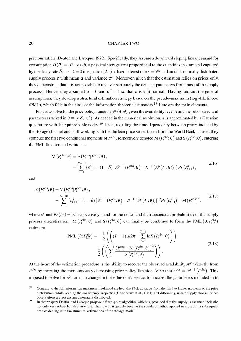
20 CHAPTER TWO
previous article (Deaton and Laroque, 1992). Specifically, they assume a downward sloping linear demand for
consumption D(P) = (P−a)/b, a physical storage cost proportional to the quantities in store and captured
by the decay rate δ ,–i.e., k = 0 in equation (2.1)–a fixed interest rate r = 5% and an i.i.d. normally distributed
supply process ε with mean µ and variance σ2. Moreover, given that the estimation relies on prices only,
they demonstrate that it is not possible to uncover separately the demand parameters from those of the supply
process. Hence, they assumed µ = 0 and σ2 = 1 so that ε is unit normal. Having laid out the general
assumptions, they develop a structural estimation strategy based on the pseudo-maximum (log)-likelihood
(PML), which falls in the class of the information-theoretic estimators.18 Here are the main elements.
First is to solve for the price policy function P (A;θ) given the availability level A and the set of structural
parameters stacked in θ ≡ (r,δ ,a,b). As needed in the numerical resolution, ε is approximated by a Gaussian
quadrature with 10 equiprobable nodes.19 Then, recalling the time-dependency between prices induced by
the storage channel and, still working with the thirteen price series taken from the World Bank dataset, they
compute the first two conditional moments of Pobs, respectively denoted M(Pobs
t ;θ)
and S(Pobs
t ;θ), entering
the PML function and written as:
M(Pobs
t ;θ)= E
(Pobs
t+1|Pobst ;θ
),
=N=10
∑n=1{εn
t+1 +(1−δ )[P−1 (Pobs
t ;θ)−D−1 (P (At ;θ))
]}Pr
(ε
nt+1),
(2.16)
and
S(Pobs
t ;θ)= V
(Pobs
t+1|Pobst ;θ
),
=N=10
∑n=1{εn
t+1 +(1−δ ) [P−1 (Pobst ;θ
)−D−1 (P (At ;θ))]}2Pr
(ε
nt+1)−M
(Pobs
t)2.
(2.17)
where εn and Pr (εn) = 0.1 respectively stand for the nodes and their associated probabilities of the supply
process discretization. M(Pobs
t ;θ)
and S(Pobs
t ;θ)
can finally be combined to form the PML(θ ;Pobs
1:T
)estimator:
PML(θ ;Pobs
1:T)=− 1
2
(((T −1) ln2π−
T−1
∑t=1
lnS(Pobs
t ;θ)))
−
12
((T−1
∑t=1
(Pobs
t+1−M(Pobs
t ;θ))2
S(Pobs
t ;θ) ))
.
(2.18)
At the heart of the estimation procedure is the ability to recover the observed availability Aobs directly from
Pobs by inverting the monotonously decreasing price policy function P so that Aobs = P−1(Pobs
t). This
imposed to solve for P for each change in the value of θ . Hence, to uncover the parameters included in θ ,
18 Contrary to the full information maximum likelihood method, the PML abstracts from the third to higher moments of the pricedistribution, while keeping the consistency properties (Gourieroux et al., 1984). Put differently, unlike supply shocks, pricesobservations are not assumed normally distributed.
19 In their papers Deaton and Laroque propose a fixed-point algorithm which is, provided that the supply is assumed inelastic,not only very robust but also very fast. That is why it quickly became the standard method applied in most of the subsequentarticles dealing with the structural estimations of the storage model.

REVIEW AND PERSPECTIVES 21
the PML optimization routine needs to nest an inner numerical algorithm for the model resolution which, as
mentioned above, makes the whole procedure computationally cumbersome.
The estimation results have been as disappointing as the approach truly innovative and inspiring since,
then again, the model fails to induce more than half of the autocorrelation levels measured in the true data,
regardless of the commodity under study. Put it another way, the transmission of shocks through the inventory
channel accounts for only a small part of the story of commodity price variations on a market driven by i.i.d.
fluctuations in production. Even more discouraging perhaps is the finding that a basic linear autoregressive
model (AR(1)) does offer a better fit. Going ahead and borrowing from Chambers and Bailey (1996), the
authors relax the assumption of an i.i.d. unit normal harvest shocks for one in which supply disturbances
followed a mere AR(1) process, denoted zt , thereby introducing an additional source of persistence in the
model dynamics.20 Looking beyond the theoretical plausibility of such a hypothesis, for instance in the case
of annual crops like grains, in spite of this richer modeling, the conclusions remain widely pessimistic as
stated by the authors themselves: “we find these results almost as disappointing as those for the storage model
with i.i.d. harvests”. Indeed, the higher levels of serial correlations obtained are almost entirely resulting
from the estimated value of ρ . All in all, the model cannot match the high degrees of serial correlation
observed in the actual price data regardless of the assumed degree of persistence in the distribution of the
supply innovations.
Still, with this methodology Deaton and Laroque definitely paved the way for future structural estimation
of the competitive storage model. Moreover, as discussed above, in the same way as the lack of power
of a statistical test can spuriously lead to reject the hypothesis of significant storage effects, the apparent
autocorrelation failure does not necessarily mean rejecting the storage theory per se. As noted in Cafiero
and Wright (2006), it rather has to do with the wrongness of part of the assumptions needed to be laid out:
the functional form of the storage cost or linear demand functions (linear, convex, constant-elasticity), the
absence of both supply reaction (production costs, capital dynamics) and demand shocks, the nature of the
innovations (e.g., size, distribution, independence) and the fixed interest rate value among others.
Besides, such a sensitivity to the model hypotheses is even confirmed by the more optimistic results
obtained from another stream of literature, initiated by Kaldor (1939) and Working (1949), and resting on the
convenience yield hypothesis. The latter is seen as the flow of services accruing to the stockholders and is
justified on the ground of timely deliveries and avoided costs either through a disruption in the manufacturing
process or thanks to the trading advantage the owner of a commodity enjoys if the price spikes-up.21 The
convenience yield prevents the occurrence of stockout situations which allows a much better fit of the
measured autocorrelation (Miranda and Rui, 1999).
20 The AR(1) process is written as zt+1 = ρzt + εt+1 with ρ the autocorrelation coefficient and ε a white noise with zero man andunit variance. It is approximated by a Markov chain limited to the 10 nodes values of ε and in which the associated transitionprobabilities are calculated so as to match a predetermined ρ . Note also that zt comes as a second state variable in the systemwhich makes the estimation trickier as proved in the associated technical paper (Deaton and Laroque, 1995).
21 Technically, it is obtained by modeling the storage cost as a marginal log-linear function of the amount stored which becomesinfinitely negative as the levels of inventories tend to zero. P∗ being infinite the constraint is never binding. Another appeal ofthis approach is to easily permit the computation of the Maximum Likelihood estimator.
22 CHAPTER TWO
However, sticking to the assumption of the non-negativity constraint on inventories, Cafiero and Wright
(2006) point to the direction of several theoretical and technical improvements to deal with this empirical
failure.
TECHNICAL ACHIEVEMENTS Building upon the Deaton and Laroque (1996)’s PML, Cafiero et al. (2011b)
demonstrate that a model with a constant marginal cost of storage which is solved with higher accuracy fits
the behavior of prices better. Considering the carrying costs proportional to the amount stored is problematic
since it makes stockholding increasingly expensive with prices. This in turn decreases the incentive to store
which is the single source of time dependency of prices in the model. As a result, the authors suggest to
set the decay rate of inventories δ to zero and estimate a constant marginal storage cost k instead. Also
crucial is the precision in the numerical approximation of the price policy function given that a substantial
part of inference relies on the accurate location of the kink at the cut-off price P∗ above which there are
no carryovers. Specifically, recalling that the lower P∗ the more time in the stockout region and the less
serial correlation generated by the model, an underestimation of P∗ entails a reduction in the model ability to
induce high levels of autocorrelation in prices.22
Michaelides and Ng (2000) compare the asymptotic properties of the PML with three simulated estimators:
the simulated methods of moments (Darrell Duffie, 1993), the efficient method of moments (Gallant and
Tauchen, 1996) and the indirect inference estimator (Gourieroux et al., 1993). Developed in the 90’s, these
computationally intensive procedures of estimation aimed at providing alternative estimators able to uncover
structural parameters of models for which there are no closed-form solutions. Through a series of Monte-
Carlo experiments, the authors show that what the PML makes up on efficiency and precision in the sense
of a smaller root mean squared error, it loses through larger estimation biases which are not decreasing
with the sample size. More precisely, it leads to overstate the decay rate δ but also to an underestimation
of the demand elasticity, the combination of the two translating into too frequent periods of zero stocks,
reducing accordingly the ability of the model to generate autocorrelation in prices. For instance, with an
annual deterioration rate of 16.9%, the estimation results for cotton imply that inventories are held only half
of the time over the 1900–1987 considered sample interval, something clearly implausible.
With this in mind, Cafiero et al. (2015) come up with a full information maximum likelihood estimator
(MLE) with better small sample performance properties and which, applied to the price of sugar, delivers a
much more optimistic view of the empirical consistency of the storage model. Although more promising the
results, trying to match the whole autocorrelation observed in the prices come at the cost of overstating the
role of storage in the formation of prices. Hence, as noted in Cafiero and Wright (2006) and further explained
in the next chapter, it might be the case that part of the serial correlation in commodity prices cannot be
accounted for by the standard storage model.
The resolution of these numerical and specification issues, in yielding much more positive conclusions
regarding the model ability to generate sufficient persistence in prices, decisively help to rekindle interests
22 According to the authors a number of points on the approximation grid in the range between 500 to 1000 appears to be sufficientas compared to the 20 to 45 points depending on the commodities used by Deaton and Laroque (1996).
REVIEW AND PERSPECTIVES 23
in the competitive storage model and the underlying theory. Having said this, as will be shown in the next
chapter, the higher autocorrelation levels can be obtained solely with very low values of demand elasticity
and storage costs k. As a result, over the whole data sample spanning from 1900 to 1987 the estimated
number of stockouts is very small if not zero. This is somewhat problematic given that the main appeal of
the storage model is precisely its faculty of delivering two regimes of prices depending whether stocks are
carried over. Together these results hint at exploring elsewhere than in the model specification and to look at
the data themselves as also suggested in Cafiero and Wright (2006). The underlying logic is simply that part
of the serial correlations in prices might have nothing to do with the storage theory and the associated transfer
of inventories, or even more broadly to any kind of economic mechanism. It is just an artifact stemming from
the way the series have been constructed and deflated. Thus, trying to fit this aspect of the price data is likely
to come at the expense of the reliability of the whole estimation procedure. Better still, in such an empirical
endeavor to test for the storage model consistency, issues related to the data are at least as important as those
regarding the model specification itself.
EMPIRICAL REFINEMENTS Guerra et al. (2015) address the potential problem of spurious time dependen-
cies due to the construction of yearly price series. Indeed, the data used thus far are a calendar averages of
monthly prices, thereby mixing spot prices from two consecutive production cycles. Working with the MLE
of Cafiero et al. (2015) on the price of corn over the period 1949–2012, they test for eight averaging methods
to construct annual price indexes, and find to really sizeable effects across the studied samples. For instance,
one of the key parameter estimates, namely the elasticity of demand for consumption, can vary by more than
a factor of two if the annual index consists in a daily average over the November month rather than over the
calendar year. On the whole they find that the best fit is obtained when using an annual value built as the
daily average over the single month of December as in Roberts and Schlenker (2013).
The second major concern is actually very standard in econometrics as it revolves around the non-
stationarity of the data.23 Specifically, the commodity prices are likely to exhibit long-run trends. An
illustration in the case of maize is given in figure 2.1. A long-run downward sloping trend is quite visible.
Another point to note is the difference in magnitudes between the very wild short-run variations in prices
with respect to the slow decreasing trend. In other words, the volatility supersedes the long-run trend, if
any, along with all the movements of lower frequencies in general. The key challenge is thus to disentangle
both components whether it is simply for testing data stationarity or when inferring parameter values. Going
beyond this preliminary crude visual inspection with formal unit root tests, I follow the strategy presented in
Ghoshray (2011) and conduct the Lee and Strazicich (2003) test which allow for shifts in the trend parameters
under both the null and the alternative, so that the rejection of the null hypothesis necessarily implies trend
stationarity. The results are reported in table 2.1.
As documented in the table, at a significance level of 10% or below, nine out of the thirteen commodities
under study are found to be trend stationary with one or two structural breaks. These findings slightly differ
from those reported by Ghoshray (2011) who runs the test on the same WB dataset but deflated by the
23 I will contend with a short summary of the various stakes given that the next chapter is entirely dedicated to the related issues.
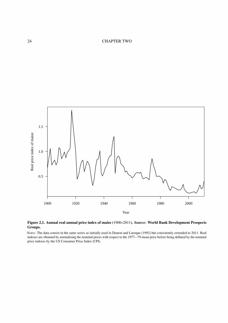
24 CHAPTER TWO
1900 1920 1940 1960 1980 2000
0.5
1.0
1.5
Year
Rea
l pric
e in
dex
of m
aize
Figure 2.1. Annual real annual price index of maize (1900–2011). Source: World Bank Development ProspectsGroups.Notes: The data consist in the same series as initially used in Deaton and Laroque (1992) but consistently extended to 2011. Realindexes are obtained by normalizing the nominal prices with respect to the 1977-–79 mean price before being deflated by the nominalprice indexes by the US Consumer Price Index (CPI).
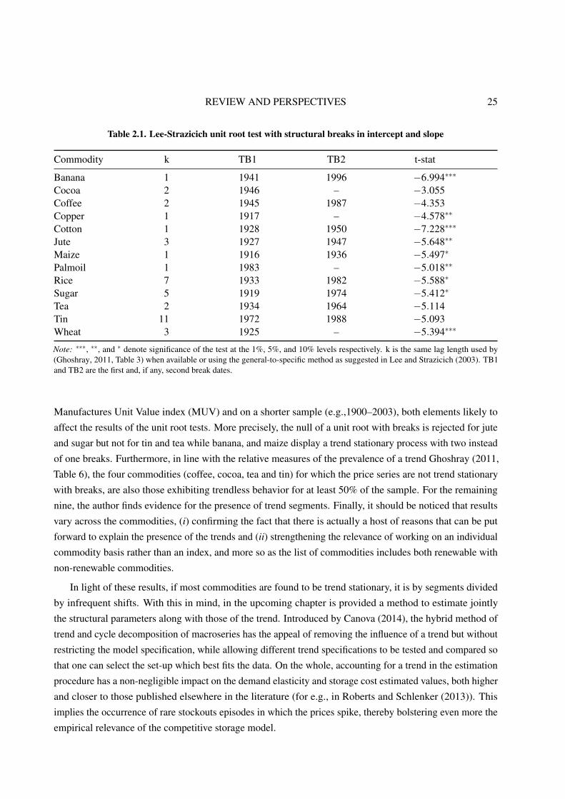
REVIEW AND PERSPECTIVES 25
Table 2.1. Lee-Strazicich unit root test with structural breaks in intercept and slope
Commodity k TB1 TB2 t-stat
Banana 1 1941 1996 −6.994∗∗∗
Cocoa 2 1946 – −3.055Coffee 2 1945 1987 −4.353Copper 1 1917 – −4.578∗∗
Cotton 1 1928 1950 −7.228∗∗∗
Jute 3 1927 1947 −5.648∗∗
Maize 1 1916 1936 −5.497∗
Palmoil 1 1983 – −5.018∗∗
Rice 7 1933 1982 −5.588∗
Sugar 5 1919 1974 −5.412∗
Tea 2 1934 1964 −5.114Tin 11 1972 1988 −5.093Wheat 3 1925 – −5.394∗∗∗
Note: ∗∗∗, ∗∗, and ∗ denote significance of the test at the 1%, 5%, and 10% levels respectively. k is the same lag length used by(Ghoshray, 2011, Table 3) when available or using the general-to-specific method as suggested in Lee and Strazicich (2003). TB1and TB2 are the first and, if any, second break dates.
Manufactures Unit Value index (MUV) and on a shorter sample (e.g.,1900–2003), both elements likely to
affect the results of the unit root tests. More precisely, the null of a unit root with breaks is rejected for jute
and sugar but not for tin and tea while banana, and maize display a trend stationary process with two instead
of one breaks. Furthermore, in line with the relative measures of the prevalence of a trend Ghoshray (2011,
Table 6), the four commodities (coffee, cocoa, tea and tin) for which the price series are not trend stationary
with breaks, are also those exhibiting trendless behavior for at least 50% of the sample. For the remaining
nine, the author finds evidence for the presence of trend segments. Finally, it should be noticed that results
vary across the commodities, (i) confirming the fact that there is actually a host of reasons that can be put
forward to explain the presence of the trends and (ii) strengthening the relevance of working on an individual
commodity basis rather than an index, and more so as the list of commodities includes both renewable with
non-renewable commodities.
In light of these results, if most commodities are found to be trend stationary, it is by segments divided
by infrequent shifts. With this in mind, in the upcoming chapter is provided a method to estimate jointly
the structural parameters along with those of the trend. Introduced by Canova (2014), the hybrid method of
trend and cycle decomposition of macroseries has the appeal of removing the influence of a trend but without
restricting the model specification, while allowing different trend specifications to be tested and compared so
that one can select the set-up which best fits the data. On the whole, accounting for a trend in the estimation
procedure has a non-negligible impact on the demand elasticity and storage cost estimated values, both higher
and closer to those published elsewhere in the literature (for e.g., in Roberts and Schlenker (2013)). This
implies the occurrence of rare stockouts episodes in which the prices spike, thereby bolstering even more the
empirical relevance of the competitive storage model.
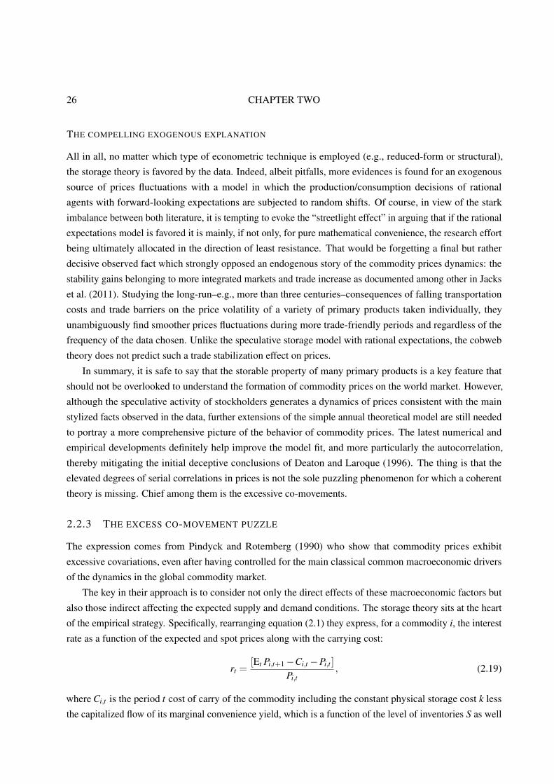
26 CHAPTER TWO
THE COMPELLING EXOGENOUS EXPLANATION
All in all, no matter which type of econometric technique is employed (e.g., reduced-form or structural),
the storage theory is favored by the data. Indeed, albeit pitfalls, more evidences is found for an exogenous
source of prices fluctuations with a model in which the production/consumption decisions of rational
agents with forward-looking expectations are subjected to random shifts. Of course, in view of the stark
imbalance between both literature, it is tempting to evoke the “streetlight effect” in arguing that if the rational
expectations model is favored it is mainly, if not only, for pure mathematical convenience, the research effort
being ultimately allocated in the direction of least resistance. That would be forgetting a final but rather
decisive observed fact which strongly opposed an endogenous story of the commodity prices dynamics: the
stability gains belonging to more integrated markets and trade increase as documented among other in Jacks
et al. (2011). Studying the long-run–e.g., more than three centuries–consequences of falling transportation
costs and trade barriers on the price volatility of a variety of primary products taken individually, they
unambiguously find smoother prices fluctuations during more trade-friendly periods and regardless of the
frequency of the data chosen. Unlike the speculative storage model with rational expectations, the cobweb
theory does not predict such a trade stabilization effect on prices.
In summary, it is safe to say that the storable property of many primary products is a key feature that
should not be overlooked to understand the formation of commodity prices on the world market. However,
although the speculative activity of stockholders generates a dynamics of prices consistent with the main
stylized facts observed in the data, further extensions of the simple annual theoretical model are still needed
to portray a more comprehensive picture of the behavior of commodity prices. The latest numerical and
empirical developments definitely help improve the model fit, and more particularly the autocorrelation,
thereby mitigating the initial deceptive conclusions of Deaton and Laroque (1996). The thing is that the
elevated degrees of serial correlations in prices is not the sole puzzling phenomenon for which a coherent
theory is missing. Chief among them is the excessive co-movements.
2.2.3 THE EXCESS CO-MOVEMENT PUZZLE
The expression comes from Pindyck and Rotemberg (1990) who show that commodity prices exhibit
excessive covariations, even after having controlled for the main classical common macroeconomic drivers
of the dynamics in the global commodity market.
The key in their approach is to consider not only the direct effects of these macroeconomic factors but
also those indirect affecting the expected supply and demand conditions. The storage theory sits at the heart
of the empirical strategy. Specifically, rearranging equation (2.1) they express, for a commodity i, the interest
rate as a function of the expected and spot prices along with the carrying cost:
rt =[Et Pi,t+1−Ci,t −Pi,t ]
Pi,t, (2.19)
where Ci,t is the period t cost of carry of the commodity including the constant physical storage cost k less
the capitalized flow of its marginal convenience yield, which is a function of the level of inventories S as well
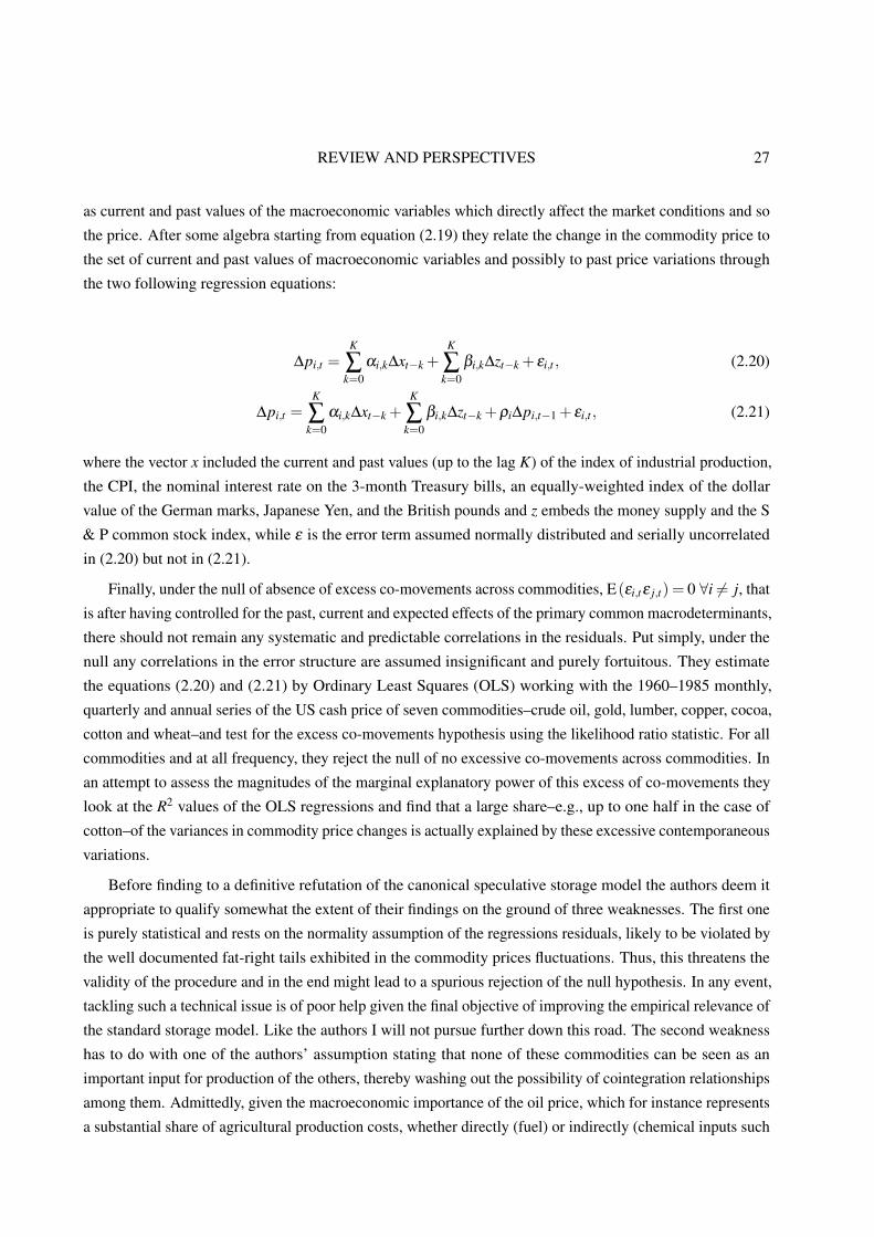
REVIEW AND PERSPECTIVES 27
as current and past values of the macroeconomic variables which directly affect the market conditions and so
the price. After some algebra starting from equation (2.19) they relate the change in the commodity price to
the set of current and past values of macroeconomic variables and possibly to past price variations through
the two following regression equations:
∆pi,t =K
∑k=0
αi,k∆xt−k +K
∑k=0
βi,k∆zt−k + εi,t , (2.20)
∆pi,t =K
∑k=0
αi,k∆xt−k +K
∑k=0
βi,k∆zt−k +ρi∆pi,t−1 + εi,t , (2.21)
where the vector x included the current and past values (up to the lag K) of the index of industrial production,
the CPI, the nominal interest rate on the 3-month Treasury bills, an equally-weighted index of the dollar
value of the German marks, Japanese Yen, and the British pounds and z embeds the money supply and the S
& P common stock index, while ε is the error term assumed normally distributed and serially uncorrelated
in (2.20) but not in (2.21).
Finally, under the null of absence of excess co-movements across commodities, E(εi,tε j,t) = 0 ∀i 6= j, that
is after having controlled for the past, current and expected effects of the primary common macrodeterminants,
there should not remain any systematic and predictable correlations in the residuals. Put simply, under the
null any correlations in the error structure are assumed insignificant and purely fortuitous. They estimate
the equations (2.20) and (2.21) by Ordinary Least Squares (OLS) working with the 1960–1985 monthly,
quarterly and annual series of the US cash price of seven commodities–crude oil, gold, lumber, copper, cocoa,
cotton and wheat–and test for the excess co-movements hypothesis using the likelihood ratio statistic. For all
commodities and at all frequency, they reject the null of no excessive co-movements across commodities. In
an attempt to assess the magnitudes of the marginal explanatory power of this excess of co-movements they
look at the R2 values of the OLS regressions and find that a large share–e.g., up to one half in the case of
cotton–of the variances in commodity price changes is actually explained by these excessive contemporaneous
variations.
Before finding to a definitive refutation of the canonical speculative storage model the authors deem it
appropriate to qualify somewhat the extent of their findings on the ground of three weaknesses. The first one
is purely statistical and rests on the normality assumption of the regressions residuals, likely to be violated by
the well documented fat-right tails exhibited in the commodity prices fluctuations. Thus, this threatens the
validity of the procedure and in the end might lead to a spurious rejection of the null hypothesis. In any event,
tackling such a technical issue is of poor help given the final objective of improving the empirical relevance of
the standard storage model. Like the authors I will not pursue further down this road. The second weakness
has to do with one of the authors’ assumption stating that none of these commodities can be seen as an
important input for production of the others, thereby washing out the possibility of cointegration relationships
among them. Admittedly, given the macroeconomic importance of the oil price, which for instance represents
a substantial share of agricultural production costs, whether directly (fuel) or indirectly (chemical inputs such
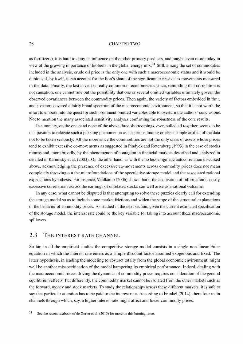
28 CHAPTER TWO
as fertilizers), it is hard to deny its influence on the other primary products, and maybe even more today in
view of the growing importance of biofuels in the global energy mix.24 Still, among the set of commodities
included in the analysis, crude oil price is the only one with such a macroeconomic status and it would be
dubious if, by itself, it can account for the lion’s share of the significant excessive co-movements measured
in the data. Finally, the last caveat is really common in econometrics since, reminding that correlation is
not causation, one cannot rule out the possibility that one or several omitted variables ultimately govern the
observed covariances between the commodity prices. Then again, the variety of factors embedded in the x
and z vectors covered a fairly broad spectrum of the macroeconomic environment, so that it is not worth the
effort to embark into the quest for such prominent omitted variables able to overturn the authors’ conclusions.
Not to mention the many associated sensitivity analyses confirming the robustness of the core results.
In summary, on the one hand none of the above three shortcomings, even pulled all together, seems to be
in a position to relegate such a puzzling phenomenon as a spurious finding or else a simple artifact of the data
not to be taken seriously. All the more since the commodities are not the only class of assets whose prices
tend to exhibit excessive co-movements as suggested in Pindyck and Rotemberg (1993) in the case of stocks
returns and, more broadly, by the phenomenon of contagion in financial markets described and analyzed in
detailed in Kaminsky et al. (2003). On the other hand, as with the no less enigmatic autocorrelation discussed
above, acknowledging the presence of excessive co-movements across commodity prices does not mean
completely throwing out the microfoundations of the speculative storage model and the associated rational
expectations hypothesis. For instance, Veldkamp (2006) shows that if the acquisition of information is costly,
excessive correlations across the earnings of unrelated stocks can well arise as a rational outcome.
In any case, what cannot be disputed is that attempting to solve these puzzles clearly call for extending
the storage model so as to include some market frictions and widen the scope of the structural explanations
of the behavior of commodity prices. As studied in the next section, given the current estimated specification
of the storage model, the interest rate could be the key variable for taking into account these macroeconomic
spillovers.
2.3 THE INTEREST RATE CHANNEL
So far, in all the empirical studies the competitive storage model consists in a single non-linear Euler
equation in which the interest rate enters as a simple discount factor assumed exogenous and fixed. The
latter hypothesis, in leading the modeling to abstract totally from the global economic environment, might
well be another misspecification of the model hampering its empirical performance. Indeed, dealing with
the macroeconomic forces driving the dynamics of commodity prices requires consideration of the general
equilibrium effects. Put differently, the commodity market cannot be isolated from the other markets such as
the forward, money and stock markets. To study the relationships across these different markets, it is safe to
say that particular attention has to be paid to the interest rate. According to Frankel (2014), there four main
channels through which, say, a higher interest rate might affect and lower commodity prices:
24 See the recent textbook of de Gorter et al. (2015) for more on this burning issue.
REVIEW AND PERSPECTIVES 29
1. a selling of inventories in response to the more costly storage activity;
2. an incentive to raise current production following the logic of the Hotelling’s principle;
3. a change in the flow of portfolio investment from the basic products into the Treasury bills;
4. an appreciation of the domestic currency leading to a decrease in the dollar denominated commodities
on the world market.
Each of these explanations are backed by theoretical developments which gave birth to specific strands of
literature. If there is certainly an element of truth to all of them, some are better supported by the data.
Furthermore, it is hard to deny the likely existence of close connections between them. For example, the
portfolio shift out of the commodity sector goes hand-in-hand with the domestic currency appreciation.
Therefore, all the econometric challenge lies in teasing-out the own contribution of each channel into the
overall variations of commodity prices. Apart from the rather intuitive and direct storage cost canal which has
already received extensive consideration, I will attempt to pick, discuss and assess both the theoretical and
empirical relevance of some of the economic mechanisms underlying the indirect effects of the interest rate
embodied by the other three channels. In the end, the aim is to build upon the competitive storage model by
painting a rough and rapid overview of some of the key macroeconomic linkages which possibly could help
to remedy both the autocorrelation and excess co-movements puzzles. Hopefully, doing this will improve the
explanatory power of the model, while keeping the storage theory at the center of the stage.
2.3.1 THE LATENT HOTELLING’S RULE
On the supply front, reckoning that until now only the mere inelastic version of the storage model has been
bought to the data, the “Hotelling’s rule” stating that the marginal value of an exhaustible resource should
grow at the rate of interest, is an appealing extension of the model albeit only meaningful for nonrenewable
resources. The point is that it thus far has been deeply rejected by the observed data (Krautkraemer, 1998).
One reason for this is that a higher interest rate is also associated with an increase in the capital cost, reducing
the rate of extraction and so the supply which, in turn, causes the price to rise. In the end it is unclear
whether an increase in the rate of interest eventually leads to raise or decrease the commodity price. In fact,
everything depends upon the “in situ” value–e.g., the difference between the price and the marginal extraction
cost–of the resource which is itself inversely related to the amount of reserves underground. This is why
a more fruitful extension perhaps would be to incorporate, in the basic storage framework, the effects of
the dynamics of investment and capital accumulation known to be particularly costly in capital intensive
industries. The last chapter of this thesis precisely deals with the interactions between investment and storage,
and demonstrates that the addition of such supply constraints in the system has material consequences on the
price behavior implied by the model. Nevertheless, as speculated in Hamilton (2009), the Hotelling’s notion
of scarcity rent raising at the rate of interest might well become more relevant in the years to come with the
depletion of the resource.
30 CHAPTER TWO
In the meantime, in light of the many possible explanations for the current empirical failure of the
Hotelling’s principle, I will not enter further into the details of why the prices of exhaustible resources have
tended to deviate from the optimal price path which would have emerged if the theory were to hold.25 Instead,
it is fair to assume that, so far, this channel has not been essential in the behavior of commodity prices and
better insights could be gained by investigating the exchange rate and monetary policy canals.
2.3.2 THE EXCHANGE RATE PASS-THROUGH
To begin with, I would like to provide a brief historical background explaining the growing importance of the
macroeconomic environment in the dynamics of commodity prices. In the wake of the break down of the
Bretton Woods monetary system and the resulting liberalization of capital and monetary markets, monetary
policy, interest rate and exchange rate have found themselves bound by the Mundell-Fleming trilemma.
Since then, interest and exchange rates are intrinsically linked within a political debate in international
macroeconomics fully polarized around the three corners of such an inconsistent trinity. Let me quickly
illustrate the way the mechanics operate with a country pegging its currency to the US dollar and not imposing
any capital controls. If, say, the US Federal Reserve raises its policy interest rate, the central bank of the
country which currency is pegged to the US dollar lost its autonomy and has to follow. Otherwise, the
resulting negative interest rates differential will entail a capital outflow towards the higher returns offered in
the US and, in turn, the local currency depreciation which eventually would break the peg with the US dollar.
A LARGE BODY OF DEDICATED LITERATURE To illuminate the various monetary, fiscal and trade policy
discussions, a huge literature emerged to assess the pass-through of exchange rates into commodity prices,
the consequences in terms of exports/imports volumes and, more broadly, the interdependence between the
financial (e.g., stocks, bonds, exchange rates), the money and commodity markets. Specifically, most of
the work in this field aims at testing the empirical validity of related theories such as the Law of One Price
(LOP), the Purchasing Power Parity (PPP), the Uncovered Interest Parity (UIP) or the rational expectations
present-value model. At first is the seminal contribution of Ridler and Yandle (1972) who depict a single-
commodity analytical framework to understand the effects of exchange rates variations on the price of an
individual primary product. This work have then been followed by studies included Schuh (1974), Chambers
and Just (1979, 1982) and Jabara and Schwartz (1987) mainly focused on the agricultural products. Finally,
the field of investigation spread to other commodities and sectors with contributions from Gilbert (1989),
Cashin and McDermott (2002) and Engel and West (2005) among others.
The overall conclusions drawn are mixed. If to very rare exceptions they all agree to sizable effects of
monetary policy and exchange rates on commodity prices, this is absolutely not the case when it comes to
assess the relative magnitudes of these impacts, in particular in terms of estimated elasticities. Moreover,
most of the time the model’s predictions are rejected. In fact, the main reasons for these empirical failures are
25 Krautkraemer (1998) provides an extensive and thorough overview of these factors which basically have to do not only withviolations from the efficient market hypotheses among which are imperfect competition, incomplete markets, externalities, butalso with the discovery of new deposits, the technological progress and the lack of data availability which makes any empiricalanalyses even more complicated.

REVIEW AND PERSPECTIVES 31
very similar to those leading to reject the storage theory and underlined earlier: the wild fluctuations in both
the observed exchange rate and commodity prices render really challenging any attempts to clearly uncover
the causalities between the variables so as to obtain precise estimates in such an unstable environment.
A good summary is provided in Chen et al. (2010) who attempt to address these major empirical caveats
of endogeneity and stationarity in relying on the concept of “commodity currency” exchange rates.26 More
precisely, concentrating on five small commodity-exporting countries–i.e., Australia, Canada, Chile, New-
Zealand and South-Africa–with floating exchange rates regimes, they embark in an in-depth empirical
analysis of the dynamic relationships between global commodity prices and exchange rates. They circumvent
the endogeneity problem inherent to all macroeconometric studies in working with a country-specific world
commodity price index whose dynamics can be reasonably assumed exogenous to those of the exchange
rates of such small open-economies.27 Regarding the stationarity concern related to possible structural shifts
in parameter values, it is alleviated in implementing the Granger causality test developed by Rossi (2005)
which, in allowing for structural breaks in the series, has proved to be robust to time-varying parameters.
In the end, they uncover a significant causal relationship, both in-sample and out-of-sample, running from
the exchange rates to the world commodity prices. Interestingly too is the finding that exchanges rates are
better in forecasting world commodity prices than the random walk with or without drift as well as the
first-order autoregressive specification which have been tested for comparison. According to the authors, this
forecasting power of exchanges rates can be explained by the very forward-looking nature of these variables
which encompass more information about the future macroeconomic conditions that what could be brought
by the others factors–e.g., output, monetary aggregate, stock market indexes–commonly introduced in the
times series regressions. Finally, they complement their analysis with a battery of robustness checks. For
instance, in obtaining similar results with the British pound instead of the US dollar, they show that the
causality uncovered is not a “dollar effect” consequence of two variables originally priced in US dollars.
All in all, the results of this study bring yet an additional evidence not only of the great influence of the
exchange rates on the behavior of global commodity prices, but also of their wide informative content about
the macroeconomic environment. There can be no doubt that it is a really good candidate for raising the
explanatory power of the commodity storage model. In my view, and from a purely speculative standpoint,
there are actually two avenues for incorporating the exchanges rates dynamics in the structural estimation of
the competitive storage model: one is exogenous while the other is endogenous.
THE DEMAND SHOCK APPROACH In this first empirical strategy, the idea consists in considering that the
monetary policy and all factors affecting the exchange rate are determined outside the commodity market
model so that it can enter the model with a reduced-form specification such as a basic AR(1). Another way
of saying that is to assume that the exchange rate is simply a sort of “manna from heaven” aggregating the
information about the macroeconomic environment and shifting the equilibrium price implied by the model,
like a long-lived demand shock in some sense.
26 The concept refers to the free-floating currencies of countries whose export revenues heavily depend on commodity exports.27 They test for potential endogeneity with an Hausmann Test. The null of exogeneity is accepted at the standard statistical levels.

32 CHAPTER TWO
For this to be done, imagine a perpetual net-exporting country of a given commodity, say Saudi-Arabia
with crude oil, selling its product to another in perpetual deficit, say the rest of the world. Under this
assumption the supply shocks do not impact the trade direction. As a result, everything goes as if both
countries equally shared the risk inherent to the uncertainty in the realized production, since any supply
disruption only affects the global amount on hand A, the unique state variable governing the commodity
price. Add to this one-way trade and perfectly risk-sharing situation the fact that, to save on trade expenses
a net-importing country never stores, and the storage and trade model described in Williams and Wright
(1991, Ch. 9) collapses into its standard version with a single country. Then, provided zero tariffs barriers
and borrowing from Chen et al. (2010) the concept of commodity currencies, there is a case for translating
the producer commodity price in the US dollars denominated international price according to the following
relationship:
Pt =
(P̃t −θ
)τt
(2.22)
where θ is the trade cost expressed in the domestic currency (the Saudi Arabian Riyal in the above example),
P and P̃ stand for the US dollar international and domestic prices respectively, while τ is the exchange rate
defined as the US dollar price of the domestic currency.
However, this “ad-hoc” statistical approach, although quite fast and easy to implement given that it only
adds one exogenous state variable (τ) to the system, does not seem able to resolve the excessive correlations
puzzle. Indeed, introducing an autocorrelated exchange rate variable is nothing but having an additional
persistent shock exactly like Deaton and Laroque (1996), but on the demand side this time. Simply put,
modeled this way the exchange rate enters the model in a similar fashion as a negative persistent supply
shock, with admittedly a more universal and convincing economic justification than its autocorrelated supply
shocks counterpart, but still identical in nature. Thus, there are good reasons to expect the estimation results
to be as discouraging as those published in Deaton and Laroque (1996), namely that the model will manage
to fit the serial correlation in prices but at the expense of attributing all the persistence to the autocorrelation
coefficient of the exchange rate. Further, since the measured excessive covariations in commodity prices
typically refers to those detected once having controlled for the exchange rates fluctuations, it does not
provide an answer at all to the excess of co-movements phenomenon.
In summary, if the unique objective is to improve the fitting performance of the storage model, then such
a model’s repair seems enough to yield satisfactory results notably in terms of induced serial correlations
in prices. Otherwise, to actually tackle the excess of covariances puzzle, there is a need for a richer
storage model specification allowing for cross-price elasticity effects between commodities and all kinds of
interconnections, feedbacks along with other linkages existing among the main macroeconomic variables
of interests. The latter only, in conveying the variety of international shocks within the structural system of
equations, hopefully can lead the model to deliver nontrivial patterns in the behavior of commodity prices,
that is going beyond the predictions based on the fundamentals alone.28 Therefore, to extend and deepen the
28 In this spirit, the Pavlova and Rigobon (2007)’s model, albeit developed in a continuous time context, is very instructive aboutthe potentiality of generating assets prices co-movements similar to those observed through the inclusion of an additional termsof trade channel in an otherwise standard international asset pricing set-up.
REVIEW AND PERSPECTIVES 33
understanding of the structural mechanisms at stakes and the directions in which the causality are running,
there is no alternative but to augment the storage model system of equations with an additional theoretical
monetary-based characterization, even very crude, which features the determination of the exchange rate.
One such theoretical framework is the model of Frankel (1986) which formalizes the theory behind the
overshooting phenomenon, a point to which I will turn now.
2.3.3 THE OVERSHOOTING THEORY
A typical illustration of what is meant by “non-trivial” patterns in the behavior of commodity prices is
certainly the overshooting concept. The core logic is completely analogous to the one embedded in the
famous overshooting model originally proposed by Dornbusch (1976) for the exchange rates. It has then
been imported in the field of commodity prices by Frankel and Hardouvelis (1985) and Frankel (1986) as a
way to feature the interdependence between the financial, money and commodity markets so as to study the
influences of the monetary policy on the dynamics of commodity prices. The key underlying assumption
is that, in response to a shift in the money supply, commodity prices adjust more rapidly than prices of
manufactured goods as has been empirically demonstrated in Bordo (1980). Reminding the storage arbitrage
condition on the expected rate of return of commodities prevailing in the commodity market, the higher
interest rate entails a fall in spot prices. However, given the stickiness of the other prices, the commodity spot
price will overshoot its expected long run equilibrium level where the general price level–e.g., consisting in
both the prices of primary and manufactured goods–has fully adjusted to the change in the money supply. In
other words, commodity prices will decline by more than proportionately to the drop in the money supply
so as to be sufficiently undervalued to offset the higher real interest rate. Hence, the expected increase in
commodity price covers the rise of the real rate of interest and induces market participants to hold inventories.
In a attempt to quantify the short-run effects subsequent to a monetary shock, Frankel (1986) combines a
money demand equation with an expectation-augmented Philips curve and the storage trade-off condition, to
derive the following relationship (keeping Frankel’s notations):
∆pc =1+λθ
1−α +λθ∆m+λ
1+λθ
1−α +λθ∆µ; (2.23)
where m is the log of money supply, pec and pm denote the logarithm of the expected commodity and
manufactured prices respectively, λ is the semi-elasticity of money demand with respect to the interest rate,
θ stands for the speed of adjustment in manufactured good markets, and µ is the secular expected rate
of inflation. Since the coefficient of ∆m is greater than one, the commodity prices will tend to overreact
following a variation in the supply of money. The latter degree of overshooting is inversely related to the
value of θ : the higher θ , the less the commodity spot price overshoots its long term value.29
From an empirical standpoint, the literature seeking to test the overshooting theory applied in the context
of commodity prices is much thinner than the one focused on the exchange rates and, as far as I know, all of
29 In the limit of an infinite θ , both commodity and manufactured goods prices instantly converged to their long-term values, thecoefficient of ∆m tends to unity and there is no overshooting.
34 CHAPTER TWO
them are reduced-from approaches. One of them is offered by Browne and Cronin (2010).30 Specifically,
using US data they apply the maximum likelihood cointegration procedure developed in Johansen (1988)
to test for the presence of the long-run dynamic relationships money, commodity and consumer prices as
posited by the theory. Embedding in a four vector autoregressive (VAR) framework with six lags, the money
stock measured by the M2 aggregate, a measure of the real GDP, the CPI, and an index of commodity
prices (three different indexes are tested), they implement the Johansen’s trace statistic test and uncover, at
either 5% or 10% levels of significance depending on the commodity price index considered, two significant
cointegrating vectors between the money stock and both the consumer and commodity price indexes.31
Using the estimated cointegrating relationships, the empirical analysis is finally supplemented by Impulse
Response Functions (IRFs) plots of the variables included in the system following a money supply shock. On
the whole, the adjustments profiles side with the theory, with the commodity price index overshooting its
long-term equilibrium level while the CPI does not. Together these results are encouraging and shed light
on the empirical relevance of the overshooting theory. Still, as mentioned by the authors themselves, their
findings in support of the overshooting theory have been obtained through a reduced form model, and thus
cannot be given any structural interpretation. All that can be said is that the predictions derived from the
theory are not at odds with the observed data.
To conclude, the overshooting theory is really attractive as it seems able to provide a theoretical ex-
planation to both the autocorrelation and the excess co-movements puzzles, while staying consistent with
the rational expectations foundations of the canonical storage model. At this juncture, the only fly in the
ointment comes from the always tricky stage of bridging the theoretical model to the data. Hence, it should
come as no surprise if, in spite of three decades of existence, there is an overall lack of empirical studies
and particularly of structural econometric works attempting to test the validity of the overshooting theory.
Part of the reason has to do with the so called “curse of dimensionality”. Indeed, as appealing and relevant
as it looks like, the integration of such monetary and macroeconomic effects within the core system of
equations of the storage model inevitably leads to an increase in the number of state variables. The thing is
that, as demonstrated in Gouel (2013a), the competitive storage model is too nonlinear to be solved with
the perturbations methods and the more numerical intensive projection techniques have to be employed
instead.32 Add to that the estimator optimization step and you get the perfect recipe for an explosion in the
computational time needed to complete the whole structural estimation procedure. All in all, addressing all
these numerical and empirical challenges is worth pursuing but very time-consuming. It turns that in the near
future one has to content with ad-hoc repairs to the competitive storage model which help improve the model
fit even though less microfounded.33 That said, the overshooting story is fairly close to be incorporated in
the storage model structure as it provides a rational explanation to the puzzling persistence and excessive
30 See also Saghaian et al. (2002) and Ching-chong et al. (2005) in the case of agriculture prices.31 The VAR is estimated assuming neither intercepts nor trends in the cointegrating vectors while the lag length has been chosen
according to the Akaike information criteria.32 They are even more computationally burdensome if you recall that the grid of approximation has to be fine enough for the price
policy function approximated with a satisfactory level of precision (Cafiero et al., 2011b).33 The alternative would be relaxing the non-negativity constraint on inventories following the convenience yield tradition.
REVIEW AND PERSPECTIVES 35
covariances in observed prices, with both a long established theoretical bedrock and a solid body of empirical
evidences.
2.4 THE OUTLOOK
In this chapter I surveyed a variety of theoretical along with empirical developments designed to provide
a structure to the analysis of commodity price volatility in the world market. This literature review helps
to isolate some key features to be considered for a sound understanding and prediction of the observed
fluctuations of prices which would prove to be helpful for informing the policy debate.
In this respect the commodity storage model with rational expectations deserves particular interest. In its
basic version, it consists in a single intertemporal storage Euler equation derived from the optimizing behavior
of speculators. Such very transparent microfoundations is not its unique asset compared to the opposed way
of modeling the behavior of commodity prices and embodied in the cobweb-type models. Indeed, when
it comes to assess their respective quantitative merits, on the whole the literature is more supportive of a
price behavior driven by the market fundamentals affected by unexpected and exogenous shocks. From the
external consistency standpoint, the superiority of the storage model has even been bolstered over the past
decade following the many important contributions achieved to address the autocorrelation puzzle along with
the other model’s empirical failures highlighted in Cafiero and Wright (2006). That said, as the short-run
volatility can also result of market exuberance, panics and irrationality, the cobweb-type models and the
complex price dynamics they can generate are still worth of existence, even though not at the center of the
political debate since, ultimately, the price reverts back to the reality dictated by the fundamentals of supply,
demand and inventories.
This is why the storage model is a good place to start thinking about commodity price volatility in offering
a common and mere core structure around which to build and organize policy discussions. In some sense, it
should be the architecture in which the relevant findings from the various fields of finance and economics are
eventually integrated, so as to improve its explanatory power and, hopefully, attempt to provide answers to
some of the current puzzling phenomenon included the persistence and the excess of co-movements in prices.
Still, to this point, it has to be noted that, so far, all the structural estimations of the storage model rest
on price information alone, which highly limit the number of parameters that can be freely identified. This
is the main reason why reasoning from a price change is of poor help when it comes to go further in the
empirical analysis with richer storage model specifications. Therefore, it is paramount in futures inference
of the storage model to draw information from both data on prices and quantities, above all now that they
begin to be available over a sufficiently long period of time.34 It is only thereafter that it will be possible to
draw reliable conclusions about the relative empirical merits of the storage theory. Moreover, confronting the
storage model with observed data on both prices and quantities will allow to assess in which dimensions the
model does and does not perform well.
34 Chapter 3 precisely tackles the challenges inherent to the structural estimations of the storage model using information onprices and quantities.

36 CHAPTER TWO
In summary, and in a pure speculative manner, a promising and realistic research agenda covering all
times frames could go like this:
ECLECTIC STORAGE MODELS in the short-run in the absence of sound theoretical microfoundations to
rely on and/or in waiting for the computational advances needed to cope with the current numerical issues,
especially those related to the curse of dimensionality discussed above. Put differently, the objective is to
improve the overall model fitting performance by embedding reduced form specification within the structural
estimation procedure to capture aspects of the data that have nothing to do with the storage theory. One such
example is the treatment of the long-run trends in commodity prices and is precisely the topic of the next
chapter.
MACROECONOMIC STORAGE MODELS in the medium-run to gradually incorporate macroeconomic forces
in a structural fashion for instance through the interest rate channel. The goal here is, without loosing any
explanatory power, to strengthen the internal consistency of the model by attempting to have as much as
possible theoretically grounded relationships across the variables in the framework. In this respect, ideally
the interdependence between the monetary policy and the commodity prices is endogenously derived in an
overshooting-type model, instead of intervening as a mere persistent demand shock imitating the broader
macroeconomic environment encapsulated in the exchange rate.
FINANCIALIZED STORAGE MODELS in the long-run to generate even richer patterns of co-movements
among commodity and assets prices. The idea is to acknowledge for spillovers effects stemming from the
financial markets flowing into the physical commodity markets, and eventually have a story for potential
speculative bubbles, self-fulfilling prophecies and other irrational behaviors of this kind. From this perspective,
the burgeoning literature on the integration of financial frictions within stochastic dynamic equilibrium models
like the competitive storage model is promising and worth of consideration. Having said this, to avoid ending
with a black-box model, it might be wiser to develop different versions of the storage model suitable for
applications under a variety of circumstances.
CHAPTER 3
ESTIMATING THE COMPETITIVE STORAGE MODEL WITH TRENDING
COMMODITY PRICES
Gustafson’s (1958) commodity storage model is fundamental for explaining the annual behavior of
commodity prices. It features forward-looking speculators that maximize profit by stockpiling a commodity
based on the difference between the expected price and the current price. The source of volatility in the
commodity storage model is the occurrence of unexpected supply shocks. The model has proven capable of
reproducing many features of commodity prices such as sharp spikes, volatility clustering, positive skewness,
and excess kurtosis (Deaton and Laroque, 1992). However, in early estimations of this model, Deaton and
Laroque (1992, 1996) show that it could not explain the high degree of serial correlation observed in the
price series. This finding was challenged. Cafiero et al. (2011b) show that using a finer grid to approximate
the policy function and a different model specification, the storage model is able to generate the observed
serial correlation for seven of the twelve commodities analyzed in Deaton and Laroque (1996). Since Cafiero
et al. (2011b), several papers provide positive evidence for the role of storage arbitrage in price behavior
(Bobenrieth et al., 2013, 2014, Cafiero et al., 2015, Guerra et al., 2015). However, if the model is estimated
on untransformed real price indexes (as in Cafiero et al., 2011b), discretionary stocks are always strictly
positive (i.e., there are no “stockouts”) for most commodities over the sample interval. This result casts doubt
on the appropriateness of using for estimation a nonlinear model with two regimes (with and without stocks)
if, over long samples and for most commodities, the estimations imply that only one regime is active.
The absence of predicted stockouts in the sample indicates a possible model misspecification. This
misspecification may arise from the attempt to fit with the storage model a serial correlation that is artificially
high, due to a possible non-stationarity in the price series. Commodity prices are unlikely to be stationary
over long periods. Starting with the work by Prebisch (1950) and Singer (1950), a large literature has been
devoted to characterizing the nature of this non-stationarity: whether trends are stochastic or deterministic,
the existence of long-run cycles, or secular decline of commodity prices relative to those of manufactures
(e.g., Grilli and Yang, 1988, Cashin and McDermott, 2002, Ghoshray, 2011, Harvey et al., 2010). As
illustrated in figure 3.1, the nature of the trends (or their absence) tends to be specific to each commodity
Chapter written with Christophe Gouel and to be published in the Journal of Applied Econometrics (DOI: 10.1002/jae.2553).
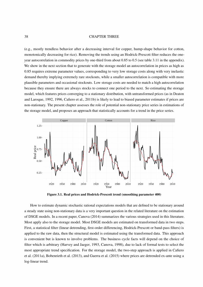
38 CHAPTER THREE
(e.g., mostly trendless behavior after a decreasing interval for copper, hump-shape behavior for cotton,
monotonically decreasing for rice). Removing the trends using an Hodrick-Prescott filter reduces the one-
year autocorrelation in commodity prices by one-third from about 0.85 to 0.5 (see table 3.11 in the appendix).
We show in the next section that to generate with the storage model an autocorrelation in prices as high as
0.85 requires extreme parameter values, corresponding to very low storage costs along with very inelastic
demand thereby implying extremely rare stockouts, while a smaller autocorrelation is compatible with more
plausible parameters and occasional stockouts. Low storage costs are needed to match a high autocorrelation
because they ensure there are always stocks to connect one period to the next. So estimating the storage
model, which features prices converging to a stationary distribution, with untransformed prices (as in Deaton
and Laroque, 1992, 1996, Cafiero et al., 2011b) is likely to lead to biased parameter estimates if prices are
non-stationary. The present chapter assesses the role of potential non-stationary price series in estimations of
the storage model, and proposes an approach that statistically accounts for a trend in the price series.
Copper Cotton Rice
0.25
0.50
0.75
1.00
1.25
1920 1950 1980 2010 1920 1950 1980 2010 1920 1950 1980 2010Year
Rea
l pric
e
Figure 3.1. Real prices and Hodrick-Prescott trend (smoothing parameter 400)
How to estimate dynamic stochastic rational expectations models that are defined to be stationary around
a steady state using non-stationary data is a very important question in the related literature on the estimation
of DSGE models. In a recent paper, Canova (2014) summarizes the various strategies used in this literature.
Most apply also to the storage model. Most DSGE models are estimated on transformed data in two steps.
First, a statistical filter (linear detrending, first-order differencing, Hodrick-Prescott or band-pass filters) is
applied to the raw data, then the structural model is estimated using the transformed data. This approach
is convenient but is known to involve problems. The business cycle facts will depend on the choice of
filter which is arbitrary (Harvey and Jaeger, 1993, Canova, 1998), due to lack of formal tests to select the
most appropriate trend specification. For the storage model, the two-step approach is applied in Cafiero
et al. (2011a), Bobenrieth et al. (2013), and Guerra et al. (2015) where prices are detrended ex-ante using a
log-linear trend.

TRENDING COMMODITY PRICES 39
Another approach involves the construction of a model that includes transitory and permanent shocks, the
latter aimed at capturing non-cyclical fluctuations. The model is made stationary by scaling the variables by
the permanent shocks, and is fitted to the raw data. This approach has the appeal of theoretical consistency
but introduces the risk of misspecification. Because it is not possible to make every model stationary for all
possible specifications of permanent shocks, the model design and the nature of the shocks may be driven
more by computational than economic motives. This approach is applied in Zeng (2012) and Bobenrieth
et al. (2014) with storage models in which storers internalize the downward trend in commodity prices and
adjust their behavior accordingly, and in Dvir and Rogoff (2014) where quantities are non-stationary, but not
prices. However, to obtain stationary equations while accounting for a trend in prices, various restrictions
must be satisfied: the trend must be multiplicative and the logarithm of the trend is restricted to take the form
of a random walk with drift; the demand function has to be isoelastic, but not linear as commonly adopted for
numerical simplicity; and storage costs must either be zero or have the same trend as prices.
Canova (2014) proposes an alternative method to estimate DSGE models using raw data.1 In this
approach, the econometrician defines a statistical model which is a combination of a DSGE and a reduced-
form model; the reduced-form is aimed at capturing the component in the data that the structural model is
unable to explain. This statistical model can be estimated using raw data, which leads to joint estimation of
the structural and reduced-form parameters. Interestingly, this one-step approach allows to select the most
likely trend specification based on a statistical criterion for model selection. Furthermore, it presents the
benefit of not restricting the trend and model specifications, but at the cost of the agents neglecting the trends
in their decisions.
The choice between the approaches amounts to a trade-off between theory and empirics. If the conditions
under which a storage model can be made stationary are too restrictive with respect to the prevailing trends,
it may not be possible to properly capture them in the model. The most severe restriction for a storage model
with trending prices is probably that the trend has to be the exponential of a random walk with drift, possibly
collapsing to a simple linear trend if the random walk step has zero length. It is unlikely to be satisfied
for most commodities. In the literature on long-run trends in commodity prices, a consensus has emerged
(Kellard and Wohar, 2006, Balagtas and Holt, 2009, Harvey et al., 2010, Ghoshray, 2011, Cuddington and
Nülle, 2014, Yamada and Yoon, 2014): (i) one can exclude a positive upward trend for commodity prices,
(ii) there is no general support for the Prebisch-Singer hypothesis of a secular deterioration with respect
to manufactured goods for all commodities, with most commodity prices actually better characterized by
discontinuous, deterministic, and non-monotonic long-term trends, possibly negative over some intervals,
and (iii) the remaining commodity prices displaying a unit root, possibly with breaks. In sum, if most
commodities are found to be trend stationary, it is by segments divided by infrequent shifts. Since a random
walk with drift would not be a satisfactory trend specification for most commodities, we adopt Canova’s
approach by jointly estimating a storage model and a reduced-form trend that describes the non-cyclical
component of price. Our approach implies that the storers neglect the existence of a trend in prices and
arbitrate prices only on the basis of their cyclical component. This issue is likely to be of second order
1 See also Ferroni (2011) for an application.
40 CHAPTER THREE
compared to the gains from making the prices more stationary (as confirmed in Zeng, 2012, who finds little
differences in estimations on small sample whether storers account for trend or not).
The estimation procedure starts from the Maximum Likelihood estimator proposed for the storage model
by Cafiero et al. (2015), and which was proved to have better small sample properties than Deaton and
Laroque’s (1996) Pseudo-Maximum Likelihood estimator. We extend the Maximum Likelihood estimator
to account for a potential trend in prices and to exploit the information available from the first observation.
This leads to the development of a new simulated unconditional Maximum Likelihood estimator. Following
the finding that most commodity prices are best characterized as trend stationary with breaks, we consider
only deterministic trend specifications. This assumption simplifies the analysis by allowing the likelihood
to be expressed analytically,2 at the cost of being inadequate for the commodity prices best characterized
as difference stationary. As well as the case without trend, we consider a multiplicative trend, in which
the logarithm of the trend can be linear as in Cafiero et al. (2011a), Bobenrieth et al. (2013, 2014), and
Guerra et al. (2015), or represented by a restricted cubic spline as in Roberts and Schlenker (2013). We
believe that by using for the trend a restricted cubic spline with up to four knots we are able to capture in
a tractable way the deterministic trends with breaks identified in the literature. For the thirteen storable
commodities considered in Deaton and Laroque (1992), there is a model with trend which presents a lower
Akaike information criterion than the model without trend. Our estimates for the preferred models more
closely replicate the key features of the data and allow for the occurrence of stockouts in line with the
observed two-regime structure of long periods of stable prices interrupted by isolated spike episodes.
The remainder of the chapter is organized as follows. Section 3.1 describes the competitive storage model
discussed and estimated in Deaton and Laroque (1992, 1996) and Cafiero et al. (2011b). Section 3.2 presents
the econometric procedure used to estimate the storage model with multiplicative deterministic trend, and
describes how the unconditional maximum likelihood estimator is constructed. Section 3.3 presents the
empirical results, and section 4.4 concludes.
3.1 THE MODEL
3.1.1 MODEL EQUATIONS
We adopt the standard competitive storage model with no supply response, constant marginal storage cost,
and no stock deterioration in line with Cafiero et al. (2011b). The exogenous supply is modeled by i.i.d.
random production shocks εt following a normal distribution with mean µ and standard deviation σ truncated
at five standard deviations. The demand for commodities consists of a demand for current consumption Ct
associated with the inverse demand function D−1 (Ct) = a+bCt , which is assumed to be linear with fixed
parameters a and b < 0, and a speculative demand from competitive risk-neutral storers. Storers carry over
St ≥ 0 units of the commodity into the next period whenever they expect a positive return to storage over the
2 Stochastic trends would require a non-linear state-space approach and the use of particle filters (Fernández-Villaverde andRubio-Ramírez, 2007), a promising but challenging approach for a model as non-linear as the storage model.
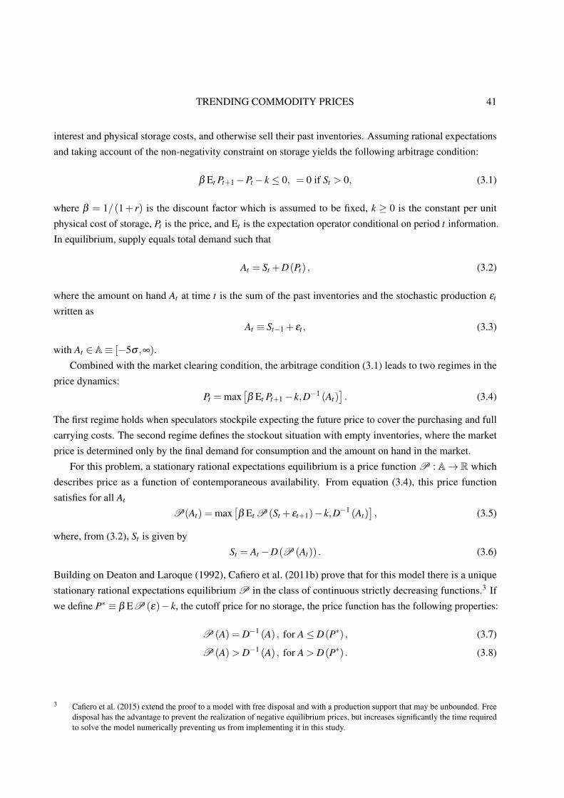
TRENDING COMMODITY PRICES 41
interest and physical storage costs, and otherwise sell their past inventories. Assuming rational expectations
and taking account of the non-negativity constraint on storage yields the following arbitrage condition:
β Et Pt+1−Pt − k ≤ 0, = 0 if St > 0, (3.1)
where β = 1/(1+ r) is the discount factor which is assumed to be fixed, k ≥ 0 is the constant per unit
physical cost of storage, Pt is the price, and Et is the expectation operator conditional on period t information.
In equilibrium, supply equals total demand such that
At = St +D(Pt) , (3.2)
where the amount on hand At at time t is the sum of the past inventories and the stochastic production εt
written as
At ≡ St−1 + εt , (3.3)
with At ∈ A≡ [−5σ ,∞).
Combined with the market clearing condition, the arbitrage condition (3.1) leads to two regimes in the
price dynamics:
Pt = max[β Et Pt+1− k,D−1 (At)
]. (3.4)
The first regime holds when speculators stockpile expecting the future price to cover the purchasing and full
carrying costs. The second regime defines the stockout situation with empty inventories, where the market
price is determined only by the final demand for consumption and the amount on hand in the market.
For this problem, a stationary rational expectations equilibrium is a price function P : A→ R which
describes price as a function of contemporaneous availability. From equation (3.4), this price function
satisfies for all At
P(At) = max[β Et P (St + εt+1)− k,D−1 (At)
], (3.5)
where, from (3.2), St is given by
St = At −D(P (At)) . (3.6)
Building on Deaton and Laroque (1992), Cafiero et al. (2011b) prove that for this model there is a unique
stationary rational expectations equilibrium P in the class of continuous strictly decreasing functions.3 If
we define P∗ ≡ β EP (ε)− k, the cutoff price for no storage, the price function has the following properties:
P (A) = D−1 (A) , for A≤ D(P∗) , (3.7)
P (A)> D−1 (A) , for A > D(P∗) . (3.8)
3 Cafiero et al. (2015) extend the proof to a model with free disposal and with a production support that may be unbounded. Freedisposal has the advantage to prevent the realization of negative equilibrium prices, but increases significantly the time requiredto solve the model numerically preventing us from implementing it in this study.

42 CHAPTER THREE
So P∗, which depends on the price function, defines the threshold between the two regimes. Prices above P∗
are too high to make storage profitable, while for prices below P∗ some stocks are carried over.
There is no closed-form solution for the equilibrium price function, which has to be approximated
numerically. The numerical method follows the fixed-point approach proposed by Deaton and Laroque
(1992) and is described in section 3.A of the appendix.
3.1.2 HOW CAN STORAGE GENERATE HIGH SERIAL CORRELATION?
The debate over the empirical relevance of the storage model revolves around its ability to generate the high
serial correlation observed in the data. Here, we explore the combination of parameters that allows the model
to generate high serial correlation. Our storage model has six parameters, {a,b,k,r,µ,σ}. In the remainder
of this chapter, we follow Deaton and Laroque (1996) and Cafiero et al. (2015) by fixing r at 5%. Deaton and
Laroque (1996, Proposition 1) prove that it is not possible to identify separately the demand function and the
distribution of supply shocks. So in this section, we set the mean and standard deviation of the harvest at 1
and 0.05.4 The mean price over the model asymptotic distribution is set to 1, which implies a+b = 1. Two
degrees of freedom remain: storage cost and demand elasticity. We vary them to see how this affects the
serial correlation. Given our assumptions, k can be interpreted as the ratio of storage costs with respect to the
mean price, and the demand elasticity calculated at the mean price is simply equal to 1/b.
To analyze the effect of storage cost on serial correlation, we set demand elasticity at −0.05, correspond-
ing to Roberts and Schlenker’s (2013) best estimate of the elasticity of a caloric aggregate of the major
crops. We vary storage costs between 0 and 20 percent of the mean price, and for every value of storage
cost we solve and simulate the model. We calculate the first-order autocorrelation for 100,000 series of 100
periods on the asymptotic distribution. As noted by Cafiero et al. (2011b), simulating the storage model
generates time series with very volatile moments when the series length is around the number of observable
annual prices (close to one hundred years). Therefore, it is not sufficient to compare the serial correlation
of observable price to the average simulated first-order autocorrelation, we need also to compare it to the
quantiles of the distribution of simulated first-order autocorrelation. The left panel of figure 3.2 displays the
5th, 50th, and 95th percentiles of the distribution of simulated first-order autocorrelation when we vary the
storage cost. Serial correlation is a monotonically decreasing function of storage cost. This can be explained
by the fact that the storage model displays two regimes. In one regime, there are positive stocks and prices
are serially correlated. In the other, stocks are zero and prices are not serially correlated. The more time
that is spent in the stockout regime, the lower will be the overall serial correlation generated by the model.
Decreasing the storage cost makes storage more profitable, increases stock levels, thereby decreasing the
likelihood of a stockout and increasing the serial correlation. With this calibration, even for a zero storage
cost, the median first-order autocorrelation is well below the very high correlation observed in the price series
(above 0.82 for all commodities except sugar). Even the 95th percentile is below 0.8.
4 A coefficient of variation of 5% for supply shocks is close to what is observed for the commodities considered in this work (seetable 3.13 in the appendix).
TRENDING COMMODITY PRICES 43
Figure 3.2. First-order autocorrelation implied by the storage model over 100 periods for several values ofstorage cost (with demand elasticity set at −0.05) and demand elasticity (with storage cost set at 0)
This failure of the storage model to induce sufficient serial correlation in prices calls for a parameterization
that is even more favorable to storage. This can be achieved by rotating the slope of the demand function
around its mean. Indeed, in absence of inventories to buffer against short supply, the price adjustments
are dictated only by the final demand for consumption. So the more inelastic the demand, the steeper the
variations in prices and the greater the incentive to store. We set the storage cost at its zero lower bound and
vary the demand elasticity between −0.4 and −0.005 (right panel of figure 3.2). Only for a very inelastic
demand curve is the median of simulated first-order autocorrelation close to 0.8. The 95th percentile can be
compatible with a first-order autocorrelation of 0.8 for a demand elasticity above −0.037.
In the storage model with i.i.d. supply shocks, stockpiling is the sole source of time-dependency in
prices, so only a model parameterization in which storage arbitrage is often active can generate high serial
correlations. The model can generate high serial correlation only by decreasing the occurrence of stockouts
which requires a parameterization of very low storage cost and very inelastic demand. So in the estimations
that follow, we should expect that a storage model able to replicate the characteristics of the raw price series
will be characterized by low storage costs and inelastic demand functions. Even with this combination, high
first-order autocorrelation is achieved only by the high percentiles of the asymptotic distribution.
3.2 ECONOMETRIC PROCEDURE
In this section, following Canova (2014), we propose an econometric procedure to estimate the storage model
and the trend in prices jointly. The idea behind this procedure is to capture in the trend the component of
prices that cannot be accounted for by the storage model, in particular the non-cyclical fluctuations. As a
result, the storage model has to account only for cyclical fluctuations in the observed data. We assume that
observed prices, Pobst , can be decomposed into a multiplicative trend exp
[Γ(t,θ Γ
)]and a cyclical component
44 CHAPTER THREE
denoted Pstot to be explained by the storage model:
Pobst = eΓ(t,θ Γ)Psto
t . (3.9)
The vector of the parameters to be estimated θ can be split into two groups: the trend parameters θ Γ, and the
structural parameters of the storage model, θ sto. In addition to the baseline case where any trend is ignored
we consider three deterministic time trend specifications. In none of the trend specifications do we introduce
an intercept because it would not be possible to identify separately the intercept of the trend from the intercept
of the inverse demand function since both would be determined by the mean level of observed prices.
3.2.1 TREND SPECIFICATIONS
NO TREND Our benchmark situation is where observed prices are assumed to be without trend. In this
case, Γ(t,θ Γ
)= 0, Pobs
t = Pstot , and θ Γ is empty.
LINEAR TREND Here we assume the trend is a deterministic linear time trend:
Γ(t,θ Γ
)= g1t. (3.10)
In this case θ Γ = {g1}. For numerical stability, the time variable, t, is taken to vary between −1 and 1.
RESTRICTED CUBIC SPLINES While the linear trend allows us to capture the overall long-run trend, it may
not capture all the non-cyclical fluctuations that the storage model is unable to explain. It is often considered
that trends in commodity prices might be non-constant (a feature captured, e.g., in Arezki et al., 2014, by
a piecewise linear trend with structural breaks). For a more flexible trend than in the linear case, we use
restricted cubic splines. Cubic splines are piecewise cubic polynomials with continuous first and second
derivatives. “Restricted” splines are splines that are constrained to be linear beyond the boundary knots
which avoids a poor behavior in the tails, a feature common to polynomial trends. A restricted cubic spline
with three knots has two parameters. With four knots, it has three parameters. So restricted cubic splines with
three and four knots have the same degrees of freedom as quadratic and cubic polynomials but tend to be
slightly more flexible. A spline with two knots would be the same as the linear trend above. Restricted cubic
splines with three to five knots are also used in Roberts and Schlenker (2013) to capture trends in prices and
quantities of agricultural commodities.
When represented by restricted cubic splines, the trend is expressed as
Γ(t,θ Γ
)=
I
∑i=1
giBi (t) , (3.11)
TRENDING COMMODITY PRICES 45
where I and Bi (·) are the degree of freedom and the basis functions of the spline,5 and gi are the trend
parameters to be estimated. The Bi (·) are functions of the knots, but once the knots are fixed the trend is
linear in its parameters. Following the heuristics proposed in Harrell (2001), the knots for the cubic spline
with three knots are located at the 10th, 50th, and 90th quantiles of the covariate, which correspond in our
1900–2011 sample to the years 1911, 1956, and 2000. The spline with four knots uses as knots the 5th, 35th,
65th, and 95th quantiles (1905, 1939, 1970, and 2006).
Since the knots are fixed before the estimation, only the slope parameters have to be estimated: θ Γ =
{gi}Ii=1.
3.2.2 THE LIKELIHOOD ESTIMATOR
Given that the price function P is strictly decreasing (Cafiero et al., 2011b), we can invert it to obtain the
amount on hand from the price. Using the inverse of the price function, the cyclical component of prices,
Psto, follows a first-order Markov process with the transition equation defined by equations (3.3) and (3.6) as
Pstot = P
(P−1 (Psto
t−1)−D
(Psto
t−1)+ εt
). (3.12)
It is possible to link Pstot to observed prices, Pobs
t , using equation (3.9). So, given the price function P ,
equations (3.9) and (4.4) define a mapping from the supply shocks εt to Pobst , conditional on Pobs
t−1 and t.
Given a set of model parameters θ and a sample of observed prices of length T , noted Pobs1:T ≡
{Pobs
1 , . . . ,PobsT}
,
and using the Markov structure of the problem, the likelihood function can be expressed as
L(θ ;Pobs
1:T)= f
(Pobs
1 ;θ) T
∏t=2
f(Pobs
t |Pobst−1;θ
). (3.13)
Using the mapping between observables and shocks, Miranda and Rui (1999) and Cafiero et al. (2015)
obtain the conditional density f(Pobs
t |Pobst−1;θ
)from the variable transformation method. Identification of the
parameters of the demand function requires the parameters of the distribution of shocks to be set to arbitrary
values. From here, the distribution of ε is assumed to be the unit normal distribution truncated at five standard
deviations, with probability density function fε (ε) = φ (ε)/ [Φ(5)−Φ(−5)] for ε ∈ [−5,5] and fε (ε) = 0
otherwise. We can write the conditional density of Pobst as:
f(Pobs
t |Pobst−1;θ
)= fε (εt) |Jt | , (3.14)
where |Jt | is the determinant of the Jacobian of the mapping Pobst 7→ εt .
5 For numerical stability, the splines are expressed in B-spline form and their basis matrices come from the command ns in the Rpackage splines.
46 CHAPTER THREE
Based on equations (3.9) and (4.4), this mapping is
εt = P−1 (Pstot)−[P−1 (Psto
t−1)−D
(Psto
t−1)],
= P−1(
e−Γ(t,θ Γ)Pobst
)−[P−1
(e−Γ(t−1,θ Γ)Pobs
t−1
)−D
(e−Γ(t−1,θ Γ)Pobs
t−1
)],
(3.15)
which gives the expression of Jt :
Jt = e−Γ(t,θ Γ)P−1′(
e−Γ(t,θ Γ)Pobst
). (3.16)
The probability of any element of Psto1:T being equal to P∗ is zero, so the derivative of P−1 exists almost
everywhere.
In this study we extend the Conditional Maximum Likelihood Estimator pioneered by Cafiero et al. (2015)
to its unconditional counterpart. The aim is to use all the available information from the first observation by
accounting for the marginal density f(Pobs
1 ;θ)
in equation (3.13). The marginal density f(Pobs
1 ;θ)
can be
expressed as the following integral over the steady-state distribution:
f(Pobs
1 ;θ)=∫
P0
f(Pobs
1 |P0;θ)
f (P0;θ)dP0. (3.17)
This integral is intractable, because there is no closed-form solution for the steady-state distribution of the
storage model. However, we can draw from the distribution with density f (P0;θ), which is the unconditional
probability density function of price in the storage model. Therefore, we can use Monte Carlo integration to
estimate f(Pobs
1 ;θ)
by simulating the model on the stationary distribution:
f(Pobs
1 ;θ)≈M−1
M
∑m=1
f(
Pobs1 |P(m)
0 ;θ
), (3.18)
where m = {1, . . . ,M} indexes random draws from the unconditional price distribution. We set the number of
draws M to 1,000,000 and obtain them by simulating 10,000 trajectories starting from the steady state for 120
periods and discarding the first 20 periods as burn-in periods. The random production shocks that generate
the price simulations are drawn at the beginning of the estimation procedure and remain fixed throughout.
Because of this simulation step, the Unconditional Maximum Likelihood Estimator falls within the class of
simulated estimators.
As is well known in time-series econometrics (Hamilton, 1994, Ch. 5), if the sample size is sufficiently
large the contribution of the first observation to the likelihood is negligible, while it is often much more
complex to calculate the unconditional likelihood than the conditional likelihood. In the case of the storage
model, it is true that the simulations necessary to calculate the marginal density make the likelihood evaluation
much more costly. In Monte Carlo experiments designed following Michaelides and Ng (2000) and Cafiero
et al. (2015), the unconditional likelihood performs only marginally better than the conditional likelihood.6
However, when using an actual sample, the unconditional likelihood has benefits which in our view outweigh
6 Results available in section 3.C of the appendix.
TRENDING COMMODITY PRICES 47
its costs. For observed prices the conditional likelihood presents many local optima. The unconditional
likelihood helps to select an optimum with an unconditional price distribution not too far from the price
sample which may not be the case for a conditional likelihood. Indeed, in order to fit the high serial correlation
of the data, the Conditional Maximum Likelihood Estimator often leads to parameter estimates for which the
availabilities corresponding to observed prices (calculated using P−1) are set at very high levels which would
correspond to very high stock levels. Observing large stock levels may have a high probability conditional on
having large stocks in the previous period, but the unconditional probability of such a situation is very low.
So, the Unconditional Maximum Likelihood Estimator helps to filter out some of these situations.
Based on all the previous elements, we can write the log-likelihood as
logL(θ ;Pobs
1:T)=−T
2log2π−T log [Φ(5)−Φ(−5)]+
T
∑t=1
[−Γ(t,θ Γ
)+ log
∣∣∣P−1′(
e−Γ(t,θ Γ)Pobst
)∣∣∣]−
T
∑t=2
(1|εt |≤5 · ε2
t +1|εt |>5 ·∞)/
2+ log
(M−1
M
∑m=1
1|ε(m)|≤5 · exp(−ε
(m)2/2))
, (3.19)
where 1 is the indicator function and ε(m) = P−1(exp(−Γ(1,θ Γ
))Pobs
1
)−S(m)
0 . Given that the interest rate
and the parameters of the distribution of production shocks have been fixed, there are three parameters that
we need to estimate for the storage model θ sto = {a,b,k}, in addition to the parameters characterizing the
trend, θ Γ, defined above. From a set of parameters θ provided by the optimization algorithm, we calculate
the detrended price Psto and solve for the policy function of the storage model P (·). Using this policy
function, we can simulate the model to calculate the marginal probability and evaluate the likelihood for this
set of parameters.
Evaluated on the observed prices, the above log-likelihood behaves badly. It displays many local optima.
Gradient-based solvers and derivative-free local search methods converge only to local optima which are
very sensitive to first guesses. Thus, we need to apply a global search algorithm to increase the likelihood
of obtaining a global solution. Following a recent review of derivative-free algorithms (Rios and Sahinidis,
2013), and some tests on our problem, we choose a global solver, the particle swarm pattern search algorithm
proposed by Vaz and Vicente (2007), and refine the solution it delivers with a local solver using a sequential
quadratic programming approach (Nocedal and Wright, 2006, Ch. 18). Parameters are constrained to remain
within bounds (this is required by the global solver). b is constrained to be strictly negative (≤−0.001) and k
to be positive or null. All the other bounds are chosen to be low enough or high enough to avoid them being
binding. The particle swarm solver is initialized with 700 vectors of first-guess parameters, a combination of
educated guesses, random draws, and vectors of previous solutions (e.g., the estimation without trend serves
as a first guess for the linear trend). The tolerance for both optimization solvers is fixed at 10−6.
Once a maximum has been identified, we estimate the asymptotic variance-covariance matrix of the
parameters as the inverse of the outer product of the scores. If the highest log-likelihood is obtained
with k constrained at its zero lower bound, calculating the variance-covariance matrix using the scores is
inappropriate, and other methods such as bootstrap should be used. However, the number of our estimations
prevents us from using the bootstrap method. For the estimates with k at zero, we do not report the standard
48 CHAPTER THREE
errors for k but report the standard errors of the other parameters obtained using the inverse of the outer
product of the scores by maintaining k at zero.
3.3 ESTIMATION RESULTS
3.3.1 DATA
Our data set is composed of the thirteen commodities analyzed in Deaton and Laroque (1992) (banana, cocoa,
coffee, copper, cotton, jute, maize, palm oil, rice, sugar, tea, tin, and wheat). The original price series from
Grilli and Yang (1988) is extended by Pfaffenzeller et al. (2007) and cover the period 1900 to 2011. The
data were downloaded from Stephan Pfaffenzeller’s personal website.7 The data are annual price indexes
calculated by averaging the monthly price data provided by the World Bank Development Prospects Groups
over the calendar year, and normalizing them with respect to the 1977–79 mean price. We deflated the
nominal price indexes by the US CPI.
We use only price data to estimate the storage model but we also rely on shorter series of production data
to illustrate the consequence of our estimations in terms of demand elasticities. The production data are from
the FAOSTAT food balance sheets in the case of the agricultural commodities,8 from the British Geological
Survey in the case of tin,9 and from the 2014 World Copper Factbook of the International Copper Study
Group for copper.10 They cover the period 1961 to 2011. For each commodity, the logarithm of production is
detrended by modeling the trend by a restricted cubic spline with five knots (as in Roberts and Schlenker,
2013).11
3.3.2 MODEL SELECTION
Joint estimation of the structural and trend parameters allows us to select the preferred trend specification
using model selection criteria. We select the preferred trend specification using the Akaike Information
Criterion (AIC). The results are reported in table 3.1 which presents the values for the preferred models in
boldface. For the model without trend the AIC is given in level, while for the three models with trend they
are given in ratios to the AIC of the model without trend so that a value above unity means a lower AIC
than the model without trend. According to the AIC, the model without trend is never retained for any of
the commodities. The model with a linear trend is preferred for copper, palm oil, and wheat. The model
with a three-knot spline trend (RCS3) is preferred for coffee, cotton, jute, rice, and sugar. The model with a
four-knot spline trend (RCS4) is preferred for banana, cocoa, maize, tea, and tin.
For the estimations where storage costs are not constrained on their lower bound we also perform
likelihood ratio tests to confirm whether the model without trend is rejected (table 3.12 in appendix). The
7 http://www.stephan-pfaffenzeller.com8 http://faostat.fao.org/9 http://www.bgs.ac.uk/mineralsuk/statistics/home.html10 http://www.icsg.org/index.php/statistics/selected-data11 The knots are located at 1964, 1975, 1986, 1998, and 2008 as suggested by Harrell (2001).
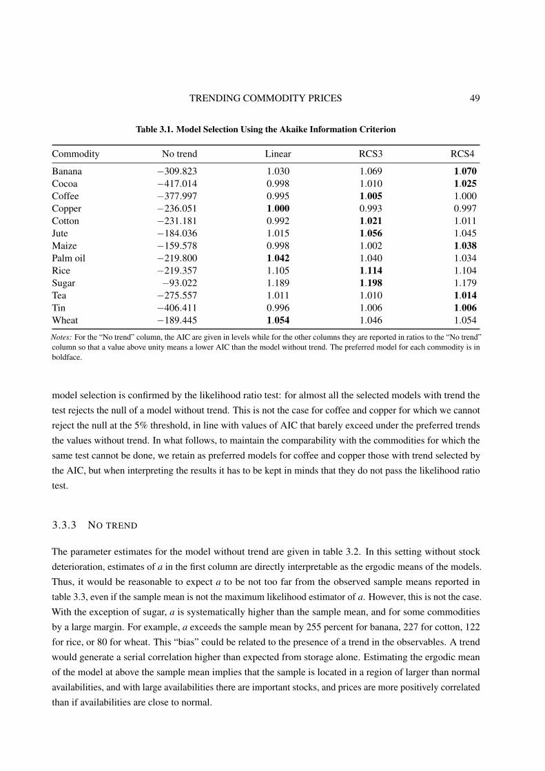
TRENDING COMMODITY PRICES 49
Table 3.1. Model Selection Using the Akaike Information Criterion
Commodity No trend Linear RCS3 RCS4
Banana −309.823 1.030 1.069 1.070Cocoa −417.014 0.998 1.010 1.025Coffee −377.997 0.995 1.005 1.000Copper −236.051 1.000 0.993 0.997Cotton −231.181 0.992 1.021 1.011Jute −184.036 1.015 1.056 1.045Maize −159.578 0.998 1.002 1.038Palm oil −219.800 1.042 1.040 1.034Rice −219.357 1.105 1.114 1.104Sugar −93.022 1.189 1.198 1.179Tea −275.557 1.011 1.010 1.014Tin −406.411 0.996 1.006 1.006Wheat −189.445 1.054 1.046 1.054
Notes: For the “No trend” column, the AIC are given in levels while for the other columns they are reported in ratios to the “No trend”column so that a value above unity means a lower AIC than the model without trend. The preferred model for each commodity is inboldface.
model selection is confirmed by the likelihood ratio test: for almost all the selected models with trend the
test rejects the null of a model without trend. This is not the case for coffee and copper for which we cannot
reject the null at the 5% threshold, in line with values of AIC that barely exceed under the preferred trends
the values without trend. In what follows, to maintain the comparability with the commodities for which the
same test cannot be done, we retain as preferred models for coffee and copper those with trend selected by
the AIC, but when interpreting the results it has to be kept in minds that they do not pass the likelihood ratio
test.
3.3.3 NO TREND
The parameter estimates for the model without trend are given in table 3.2. In this setting without stock
deterioration, estimates of a in the first column are directly interpretable as the ergodic means of the models.
Thus, it would be reasonable to expect a to be not too far from the observed sample means reported in
table 3.3, even if the sample mean is not the maximum likelihood estimator of a. However, this is not the case.
With the exception of sugar, a is systematically higher than the sample mean, and for some commodities
by a large margin. For example, a exceeds the sample mean by 255 percent for banana, 227 for cotton, 122
for rice, or 80 for wheat. This “bias” could be related to the presence of a trend in the observables. A trend
would generate a serial correlation higher than expected from storage alone. Estimating the ergodic mean
of the model at above the sample mean implies that the sample is located in a region of larger than normal
availabilities, and with large availabilities there are important stocks, and prices are more positively correlated
than if availabilities are close to normal.
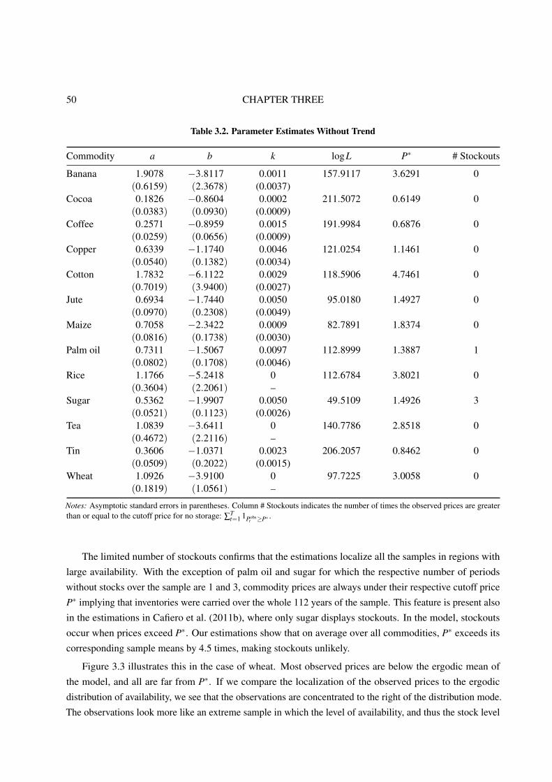
50 CHAPTER THREE
Table 3.2. Parameter Estimates Without Trend
Commodity a b k logL P∗ # Stockouts
Banana 1.9078 −3.8117 0.0011 157.9117 3.6291 0(0.6159) (2.3678) (0.0037)
Cocoa 0.1826 −0.8604 0.0002 211.5072 0.6149 0(0.0383) (0.0930) (0.0009)
Coffee 0.2571 −0.8959 0.0015 191.9984 0.6876 0(0.0259) (0.0656) (0.0009)
Copper 0.6339 −1.1740 0.0046 121.0254 1.1461 0(0.0540) (0.1382) (0.0034)
Cotton 1.7832 −6.1122 0.0029 118.5906 4.7461 0(0.7019) (3.9400) (0.0027)
Jute 0.6934 −1.7440 0.0050 95.0180 1.4927 0(0.0970) (0.2308) (0.0049)
Maize 0.7058 −2.3422 0.0009 82.7891 1.8374 0(0.0816) (0.1738) (0.0030)
Palm oil 0.7311 −1.5067 0.0097 112.8999 1.3887 1(0.0802) (0.1708) (0.0046)
Rice 1.1766 −5.2418 0 112.6784 3.8021 0(0.3604) (2.2061) –
Sugar 0.5362 −1.9907 0.0050 49.5109 1.4926 3(0.0521) (0.1123) (0.0026)
Tea 1.0839 −3.6411 0 140.7786 2.8518 0(0.4672) (2.2116) –
Tin 0.3606 −1.0371 0.0023 206.2057 0.8462 0(0.0509) (0.2022) (0.0015)
Wheat 1.0926 −3.9100 0 97.7225 3.0058 0(0.1819) (1.0561) –
Notes: Asymptotic standard errors in parentheses. Column # Stockouts indicates the number of times the observed prices are greaterthan or equal to the cutoff price for no storage: ∑
Tt=1 1Pobs
t ≥P∗ .
The limited number of stockouts confirms that the estimations localize all the samples in regions with
large availability. With the exception of palm oil and sugar for which the respective number of periods
without stocks over the sample are 1 and 3, commodity prices are always under their respective cutoff price
P∗ implying that inventories were carried over the whole 112 years of the sample. This feature is present also
in the estimations in Cafiero et al. (2011b), where only sugar displays stockouts. In the model, stockouts
occur when prices exceed P∗. Our estimations show that on average over all commodities, P∗ exceeds its
corresponding sample means by 4.5 times, making stockouts unlikely.
Figure 3.3 illustrates this in the case of wheat. Most observed prices are below the ergodic mean of
the model, and all are far from P∗. If we compare the localization of the observed prices to the ergodic
distribution of availability, we see that the observations are concentrated to the right of the distribution mode.
The observations look more like an extreme sample in which the level of availability, and thus the stock level
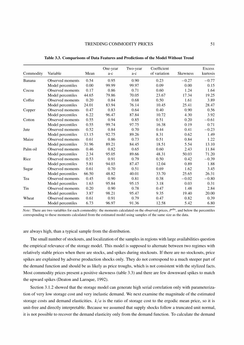
TRENDING COMMODITY PRICES 51
Table 3.3. Comparisons of Data Features and Predictions of the Model Without Trend
One-year Two-year Coefficient ExcessCommodity Variable Mean a-c a-c of variation Skewness kurtosis
Banana Observed moments 0.54 0.95 0.90 0.23 −0.27 −0.77Model percentiles 0.00 99.99 99.97 0.09 0.00 0.15
Cocoa Observed moments 0.17 0.86 0.71 0.60 1.24 1.64Model percentiles 44.65 79.86 70.05 23.67 17.34 19.25
Coffee Observed moments 0.20 0.84 0.68 0.50 1.61 3.89Model percentiles 24.01 83.94 76.14 10.45 25.41 28.47
Copper Observed moments 0.47 0.83 0.64 0.40 0.90 0.56Model percentiles 6.22 96.47 87.84 10.72 4.30 3.92
Cotton Observed moments 0.55 0.94 0.85 0.51 0.20 −0.61Model percentiles 0.55 99.74 97.75 16.38 0.19 0.71
Jute Observed moments 0.52 0.84 0.70 0.44 0.41 −0.23Model percentiles 13.15 92.75 89.26 8.31 0.62 1.49
Maize Observed moments 0.61 0.86 0.73 0.51 0.84 1.22Model percentiles 31.96 89.21 84.45 18.51 5.54 13.10
Palm oil Observed moments 0.46 0.82 0.65 0.60 2.43 11.84Model percentiles 2.34 95.05 89.66 48.31 50.03 71.20
Rice Observed moments 0.53 0.91 0.79 0.50 0.42 −0.39Model percentiles 5.81 94.03 87.47 12.04 0.89 1.88
Sugar Observed moments 0.61 0.70 0.51 0.69 1.62 3.45Model percentiles 66.50 48.82 40.01 33.70 25.65 26.31
Tea Observed moments 0.45 0.90 0.81 0.38 −0.02 −0.80Model percentiles 1.63 95.84 95.15 3.18 0.03 0.31
Tin Observed moments 0.20 0.90 0.78 0.47 1.48 2.84Model percentiles 3.87 98.21 95.47 9.35 19.40 20.00
Wheat Observed moments 0.61 0.91 0.79 0.47 0.82 0.39Model percentiles 6.73 96.97 91.36 12.58 5.42 6.80
Note: There are two variables for each commodity: the moments calculated on the observed prices, Pobs, and below the percentilescorresponding to these moments calculated from the estimated model using samples of the same size as the data.
are always high, than a typical sample from the distribution.
The small number of stockouts, and localization of the samples in regions with large availabilities question
the empirical relevance of the storage model. This model is supposed to alternate between two regimes with
relatively stable prices when there are stocks, and spikes during stockouts. If there are no stockouts, price
spikes are explained by adverse production shocks only. They do not correspond to a much steeper part of
the demand function and should be as likely as price troughs, which is not consistent with the stylized facts.
Most commodity prices present a positive skewness (table 3.3) and there are few downward spikes to match
the upward spikes (Deaton and Laroque, 1992).
Section 3.1.2 showed that the storage model can generate high serial correlation only with parameteriza-
tion of very low storage cost and very inelastic demand. We next examine the magnitude of the estimated
storage costs and demand elasticities. k/a is the ratio of storage cost to the ergodic mean price, so it is
unit-free and directly interpretable. Because we assumed that supply shocks follow a truncated unit normal,
it is not possible to recover the demand elasticity only from the demand function. To calculate the demand
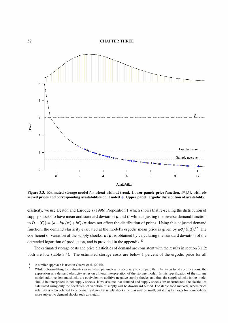
52 CHAPTER THREE
Figure 3.3. Estimated storage model for wheat without trend. Lower panel: price function, P (A), with ob-served prices and corresponding availabilities on it noted +. Upper panel: ergodic distribution of availability.
elasticity, we use Deaton and Laroque’s (1996) Proposition 1 which shows that re-scaling the distribution of
supply shocks to have mean and standard deviation µ and σ while adjusting the inverse demand function
to D̃−1 (Ct) = (a−bµ/σ)+bCt/σ does not affect the distribution of prices. Using this adjusted demand
function, the demand elasticity evaluated at the model’s ergodic mean price is given by aσ/(bµ).12 The
coefficient of variation of the supply shocks, σ/µ , is obtained by calculating the standard deviation of the
detrended logarithm of production, and is provided in the appendix.13
The estimated storage costs and price elasticities of demand are consistent with the results in section 3.1.2:
both are low (table 3.4). The estimated storage costs are below 1 percent of the ergodic price for all
12 A similar approach is used in Guerra et al. (2015).13 While reformulating the estimates as unit-free parameters is necessary to compare them between trend specifications, the
expression as a demand elasticity relies on a literal interpretation of the storage model. In this specification of the storagemodel, additive demand shocks are equivalent to additive negative supply shocks, and thus the supply shocks in the modelshould be interpreted as net-supply shocks. If we assume that demand and supply shocks are uncorrelated, the elasticitiescalculated using only the coefficient of variation of supply will be downward biased. For staple food markets, where pricevolatility is often believed to be primarily driven by supply shocks the bias may be small, but it may be larger for commoditiesmore subject to demand shocks such as metals.
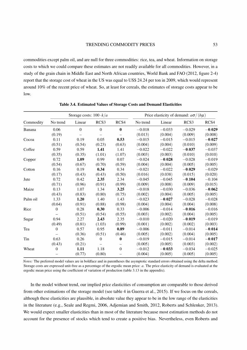
TRENDING COMMODITY PRICES 53
commodities except palm oil, and are null for three commodities: rice, tea, and wheat. Information on storage
costs to which we could compare these estimates are not readily available for all commodities. However, in a
study of the grain chain in Middle East and North African countries, World Bank and FAO (2012, figure 2-4)
report that the storage cost of wheat in the US was equal to US$ 24.24 per ton in 2009, which would represent
around 10% of the recent price of wheat. So, at least for cereals, the estimates of storage costs appear to be
low.
Table 3.4. Estimated Values of Storage Costs and Demand Elasticities
Storage costs: 100 · k/a Price elasticity of demand: aσ/(bµ)
Commodity No trend Linear RCS3 RCS4 No trend Linear RCS3 RCS4
Banana 0.06 0 0 0 −0.018 −0.033 −0.029 −0.029(0.19) – – – (0.013) (0.004) (0.009) (0.008)
Cocoa 0.11 0.19 0.05 0.53 −0.015 −0.015 −0.015 −0.027(0.51) (0.54) (0.23) (0.63) (0.004) (0.004) (0.010) (0.009)
Coffee 0.59 0.59 1.41 1.41 −0.022 −0.022 −0.037 −0.037(0.35) (0.35) (1.01) (1.07) (0.003) (0.003) (0.010) (0.010)
Copper 0.72 1.09 0.99 0.07 −0.024 −0.028 −0.028 −0.019(0.54) (0.67) (0.70) (0.59) (0.004) (0.004) (0.005) (0.005)
Cotton 0.16 0.19 0.34 0.34 −0.021 −0.022 −0.029 −0.029(0.17) (0.43) (0.43) (0.50) (0.016) (0.038) (0.015) (0.020)
Jute 0.72 0.42 2.35 2.34 −0.045 −0.045 −0.104 −0.104(0.71) (0.96) (0.91) (0.99) (0.009) (0.008) (0.009) (0.015)
Maize 0.13 1.07 1.34 3.25 −0.018 −0.030 −0.036 −0.062(0.43) (0.83) (0.80) (0.75) (0.002) (0.004) (0.005) (0.005)
Palm oil 1.33 1.20 1.40 1.43 −0.023 −0.027 −0.028 −0.028(0.64) (0.91) (0.88) (0.98) (0.004) (0.004) (0.004) (0.008)
Rice 0 0.28 0.30 0.33 −0.006 −0.014 −0.016 −0.016– (0.51) (0.54) (0.55) (0.003) (0.002) (0.004) (0.005)
Sugar 0.94 2.27 2.43 2.35 −0.010 −0.020 −0.019 −0.019(0.49) (0.81) (1.03) (0.99) (0.001) (0.002) (0.002) (0.003)
Tea 0 0.57 0.95 0.89 −0.006 −0.011 −0.014 −0.014– (0.36) (0.51) (0.46) (0.005) (0.002) (0.004) (0.005)
Tin 0.63 0.26 0 0 −0.019 −0.015 −0.014 −0.017(0.43) (0.21) – – (0.005) (0.005) (0.003) (0.002)
Wheat 0 1.11 1.18 0 −0.012 −0.033 −0.034 −0.025– (0.77) (0.80) – (0.004) (0.005) (0.005) (0.005)
Notes: The preferred model values are in boldface and in parentheses the asymptotic standard errors obtained using the delta method.Storage costs are expressed unit-free as a percentage of the ergodic mean price: a. The price elasticity of demand is evaluated at theergodic mean price using the coefficient of variation of production (table 3.13 in the appendix).
In the model without trend, our implied price elasticities of consumption are comparable to those derived
from other estimations of the storage model (see table 4 in Guerra et al., 2015). If we focus on the cereals,
although these elasticities are plausible, in absolute value they appear to be in the low range of the elasticities
in the literature (e.g., Seale and Regmi, 2006, Adjemian and Smith, 2012, Roberts and Schlenker, 2013).
We would expect smaller elasticities than in most of the literature because most estimation methods do not
account for the presence of stocks which tend to create a positive bias. Nevertheless, even Roberts and
54 CHAPTER THREE
Schlenker (2013) who control for the effect of storage using instrumental variables find higher elasticities of
demand, between −0.066 and −0.028 for aggregate calories from maize, rice, soybeans and wheat, and even
higher values for each commodity individually.
3.3.4 MODELS WITH A TIME TREND
The parameter estimates for the model with a linear trend are given in table 3.5. Since for numerical stability
the time variable has been defined over the interval [−1,1], the trend coefficient g1 is not directly interpretable.
To make it interpretable, we report it also as annual growth rates in column G, where the standard deviation is
calculated using the Delta method. For all commodities except tin, the annual growth rate is negative, which
is consistent with the Prebisch-Singer hypothesis of a long-run downward trend in commodity prices. If we
exclude coffee and tin, the values range from an annual decline of 0.4 percent for copper to 1.94 percent
for rice. The significance of many trend coefficients indicates that the model without trend is likely to be
misspecified.
For the other trend specifications, since the trend and the structural parameters are not directly inter-
pretable, the complete results are not displayed here. They are provided in the appendix, along with a
figure plotting the various trends with real prices. Rather than presenting detailed results, table 3.4 presents
the parameters estimates expressed in a way that makes them comparable across trend specifications. The
presence of a deterministic time trend in the model estimation can lead to large effects in terms of the key
parameter estimates. Storage costs tend to increase when there is a trend, and also price elasticity of demand
in absolute value. With the preferred model (in boldface) ten out of the thirteen commodities present higher
storage costs than if there is no trend. With the exception of tin, all price elasticities are higher with the
preferred model. The differences between the elasticities estimated with the models without trend and with
the preferred models with trend are important. The elasticities double in the case of cocoa, coffee, jute, rice,
sugar, and tea, and increase three-fold for maize and wheat.
For cereals, the elasticities of the preferred model although still low appear to be more consistent with
the literature. Similarly, the increase in storage costs for cereals leads to more plausible parameters which
nevertheless are low compared to some published figures.
For sugar, we can compare the parameter estimates to the Conditional Maximum Likelihood estimates of
Cafiero et al. (2015). They estimate their model on data from 1921 to 2009, because of a possible structural
break between 1920 and 1921. On this subsample, the stationarity of deflated prices is more likely to hold
(see figure 3.4 in the appendix) and the first-order autocorrelation at 0.63 is lower than the 0.70 obtained over
our extended sample. The purpose of our joint estimation approach is precisely to accommodate for such
possible breaks. The preferred model for sugar is the model with a three-knot spline trend. The estimated
trend is decreasing at the beginning of the sample and roughly constant after 1930 (figure 3.4 in the appendix).
We express the parameters in ratios to make them comparable across specifications. For 100 · k/a, our
estimation is 2.43 (table 3.14 in the appendix) and theirs is 2.23 (Cafiero et al., 2015, Table 3, ML setting
d = 0). For a/b, our estimation is −0.52 and theirs is −0.49. The estimations are very close, while they
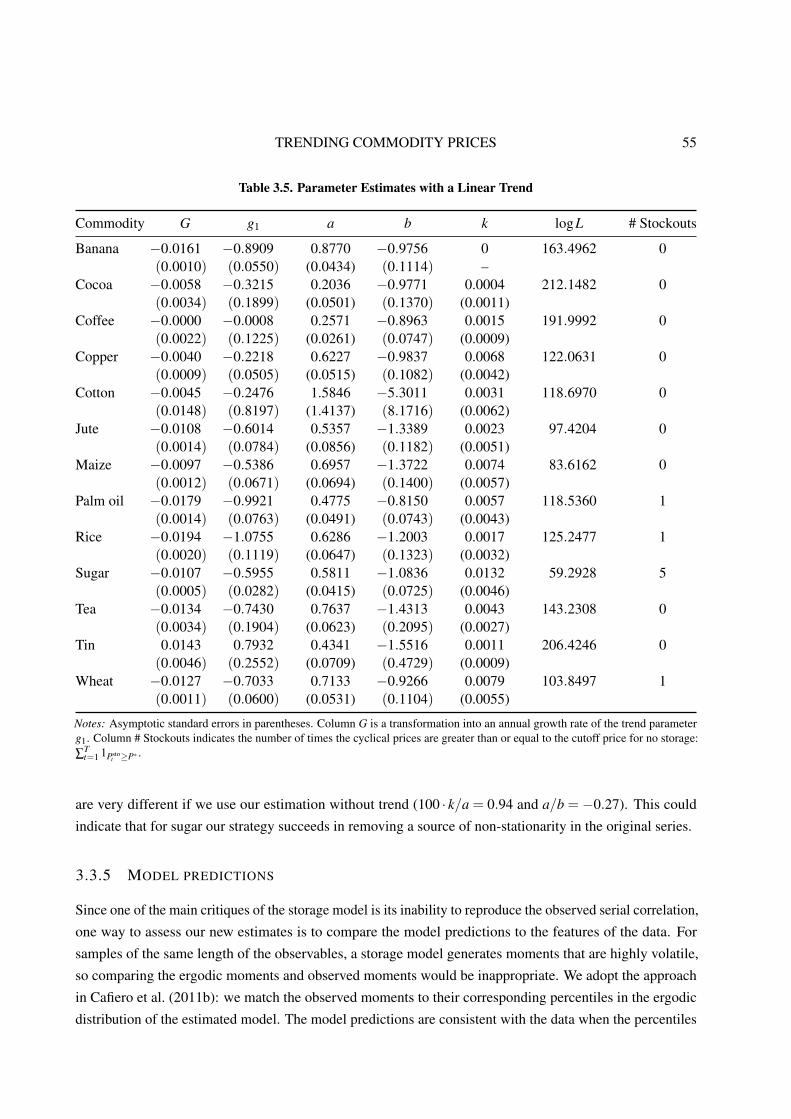
TRENDING COMMODITY PRICES 55
Table 3.5. Parameter Estimates with a Linear Trend
Commodity G g1 a b k logL # Stockouts
Banana −0.0161 −0.8909 0.8770 −0.9756 0 163.4962 0(0.0010) (0.0550) (0.0434) (0.1114) –
Cocoa −0.0058 −0.3215 0.2036 −0.9771 0.0004 212.1482 0(0.0034) (0.1899) (0.0501) (0.1370) (0.0011)
Coffee −0.0000 −0.0008 0.2571 −0.8963 0.0015 191.9992 0(0.0022) (0.1225) (0.0261) (0.0747) (0.0009)
Copper −0.0040 −0.2218 0.6227 −0.9837 0.0068 122.0631 0(0.0009) (0.0505) (0.0515) (0.1082) (0.0042)
Cotton −0.0045 −0.2476 1.5846 −5.3011 0.0031 118.6970 0(0.0148) (0.8197) (1.4137) (8.1716) (0.0062)
Jute −0.0108 −0.6014 0.5357 −1.3389 0.0023 97.4204 0(0.0014) (0.0784) (0.0856) (0.1182) (0.0051)
Maize −0.0097 −0.5386 0.6957 −1.3722 0.0074 83.6162 0(0.0012) (0.0671) (0.0694) (0.1400) (0.0057)
Palm oil −0.0179 −0.9921 0.4775 −0.8150 0.0057 118.5360 1(0.0014) (0.0763) (0.0491) (0.0743) (0.0043)
Rice −0.0194 −1.0755 0.6286 −1.2003 0.0017 125.2477 1(0.0020) (0.1119) (0.0647) (0.1323) (0.0032)
Sugar −0.0107 −0.5955 0.5811 −1.0836 0.0132 59.2928 5(0.0005) (0.0282) (0.0415) (0.0725) (0.0046)
Tea −0.0134 −0.7430 0.7637 −1.4313 0.0043 143.2308 0(0.0034) (0.1904) (0.0623) (0.2095) (0.0027)
Tin 0.0143 0.7932 0.4341 −1.5516 0.0011 206.4246 0(0.0046) (0.2552) (0.0709) (0.4729) (0.0009)
Wheat −0.0127 −0.7033 0.7133 −0.9266 0.0079 103.8497 1(0.0011) (0.0600) (0.0531) (0.1104) (0.0055)
Notes: Asymptotic standard errors in parentheses. Column G is a transformation into an annual growth rate of the trend parameterg1. Column # Stockouts indicates the number of times the cyclical prices are greater than or equal to the cutoff price for no storage:∑
Tt=1 1Psto
t ≥P∗ .
are very different if we use our estimation without trend (100 · k/a = 0.94 and a/b = −0.27). This could
indicate that for sugar our strategy succeeds in removing a source of non-stationarity in the original series.
3.3.5 MODEL PREDICTIONS
Since one of the main critiques of the storage model is its inability to reproduce the observed serial correlation,
one way to assess our new estimates is to compare the model predictions to the features of the data. For
samples of the same length of the observables, a storage model generates moments that are highly volatile,
so comparing the ergodic moments and observed moments would be inappropriate. We adopt the approach
in Cafiero et al. (2011b): we match the observed moments to their corresponding percentiles in the ergodic
distribution of the estimated model. The model predictions are consistent with the data when the percentiles
56 CHAPTER THREE
are neither too low nor too high. We calculate the mean, first- and second-order autocorrelations, coefficient of
variation, skewness, and kurtosis for the observations. For the model with trend, the moments are calculated
on the cyclical component of prices, Psto, which is the component that the storage model is supposed to
explain. We calculate the corresponding percentiles using 1,000,000 series of 112 periods from the asymptotic
distribution.
The moments and their localization with respect to simulated percentiles are given in table 3.3 for the
model without trend and in table 3.6 for the preferred model with trend. All moments from the observations
are located within the implied empirical distribution of the models without and with trend. As already noted
by Cafiero et al. (2011b), if the model without trend is solved and estimated with a sufficiently precise grid, it
is able to generate first-order autocorrelation similar to the observations for several commodities (table 3.3),
but except for sugar the observed autocorrelation corresponds to high model percentiles. The storage model
even appears to fail more often to reproduce the skewness and kurtosis, with observed moments which are
frequently below the 0.5 and 2.5 percentiles calculated from the estimated model. It should be noted that the
banana and tea price series present negative skewness, which makes them nearly impossible to reproduce
with a storage model which on average generates positive skewness. When a commodity presents negative
excess kurtosis, which is the case of banana, cotton, jute, rice and tea, it seems that the estimated model has
difficulty reproducing it. Deaton and Laroque (1992, section 2.1) note that the storage model can produce
negative excess kurtosis but only from a calibration with low price volatility and a limited role for storage,
which does not correspond to our estimations.
We turn next to the predictions of the preferred model with trend (table 3.6). Compared to the model
without trend, several commodities show an improvement in the model predictions with many moments
closer to central percentiles. However, the predictions for some commodities – banana, jute, and tea – do
not improve. The storage model with the specifications we estimated seems unable to match the moments
for these three commodities. Due to the deterministic trend, observed first-order autocorrelation decreases
but does not become systematically more consistent with the model predictions, because with estimations
of higher storage costs and more elastic demand the capacity of the storage model to generate high serial
correlation decreases also. For cocoa and maize, the percentiles corresponding to the observed first-order
autocorrelation increase significantly toward higher values indicating a decrease in the ability of the model to
reproduce this moment. Regarding the second-order autocorrelation, the skewness, and the excess kurtosis,
the preferred detrended models are much more able to fit the observed moments than the models without
trend. Similarly, if we exclude banana, jute and tea, and with the exception of 3 moments that are outside
of the (2.5,97.5) percentiles, all other moments are consistent with the predictions of the estimated storage
models.
A disturbing feature of the estimations without trend is the very small number (often zero) of implied
stockouts. Considering the possibility of a trend increases the number of implied stockouts, which becomes
positive for many commodities (table 3.7). However, even if we exclude banana, jute and tea, three
commodities – cocoa, copper, and cotton – present zero stockouts.
It is interesting to compare the number of implied stockouts to the probabilities of exceeding a given
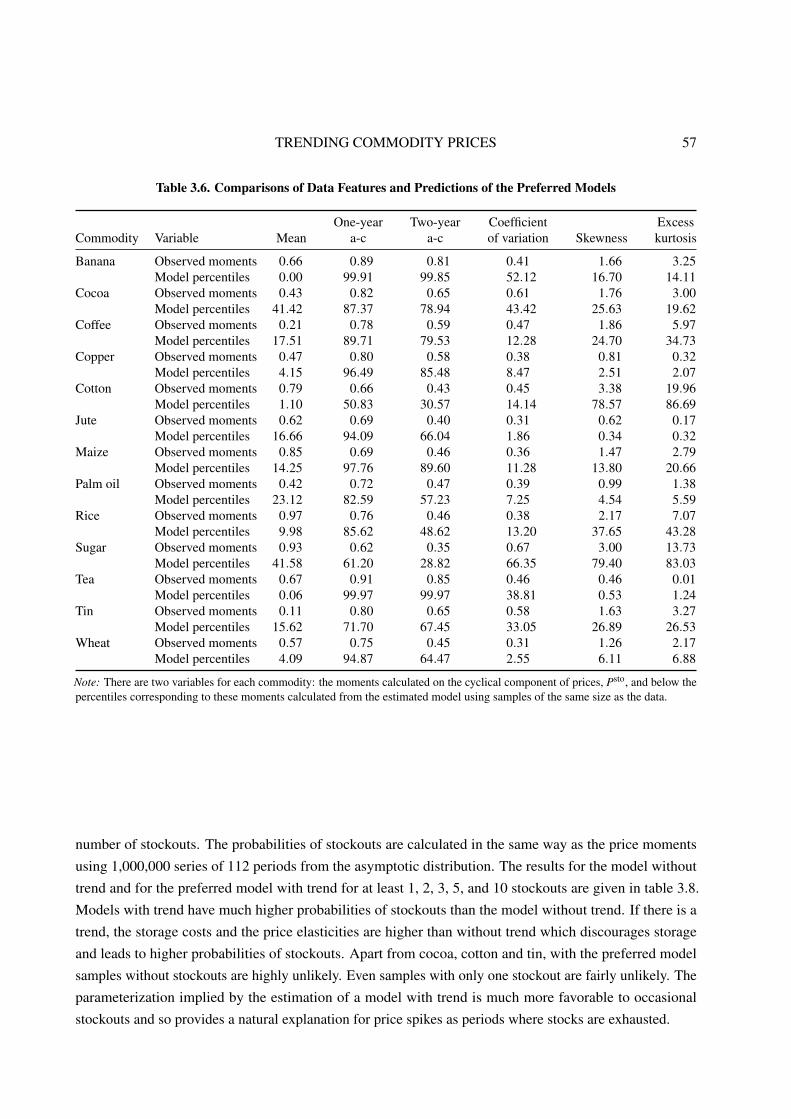
TRENDING COMMODITY PRICES 57
Table 3.6. Comparisons of Data Features and Predictions of the Preferred Models
One-year Two-year Coefficient ExcessCommodity Variable Mean a-c a-c of variation Skewness kurtosis
Banana Observed moments 0.66 0.89 0.81 0.41 1.66 3.25Model percentiles 0.00 99.91 99.85 52.12 16.70 14.11
Cocoa Observed moments 0.43 0.82 0.65 0.61 1.76 3.00Model percentiles 41.42 87.37 78.94 43.42 25.63 19.62
Coffee Observed moments 0.21 0.78 0.59 0.47 1.86 5.97Model percentiles 17.51 89.71 79.53 12.28 24.70 34.73
Copper Observed moments 0.47 0.80 0.58 0.38 0.81 0.32Model percentiles 4.15 96.49 85.48 8.47 2.51 2.07
Cotton Observed moments 0.79 0.66 0.43 0.45 3.38 19.96Model percentiles 1.10 50.83 30.57 14.14 78.57 86.69
Jute Observed moments 0.62 0.69 0.40 0.31 0.62 0.17Model percentiles 16.66 94.09 66.04 1.86 0.34 0.32
Maize Observed moments 0.85 0.69 0.46 0.36 1.47 2.79Model percentiles 14.25 97.76 89.60 11.28 13.80 20.66
Palm oil Observed moments 0.42 0.72 0.47 0.39 0.99 1.38Model percentiles 23.12 82.59 57.23 7.25 4.54 5.59
Rice Observed moments 0.97 0.76 0.46 0.38 2.17 7.07Model percentiles 9.98 85.62 48.62 13.20 37.65 43.28
Sugar Observed moments 0.93 0.62 0.35 0.67 3.00 13.73Model percentiles 41.58 61.20 28.82 66.35 79.40 83.03
Tea Observed moments 0.67 0.91 0.85 0.46 0.46 0.01Model percentiles 0.06 99.97 99.97 38.81 0.53 1.24
Tin Observed moments 0.11 0.80 0.65 0.58 1.63 3.27Model percentiles 15.62 71.70 67.45 33.05 26.89 26.53
Wheat Observed moments 0.57 0.75 0.45 0.31 1.26 2.17Model percentiles 4.09 94.87 64.47 2.55 6.11 6.88
Note: There are two variables for each commodity: the moments calculated on the cyclical component of prices, Psto, and below thepercentiles corresponding to these moments calculated from the estimated model using samples of the same size as the data.
number of stockouts. The probabilities of stockouts are calculated in the same way as the price moments
using 1,000,000 series of 112 periods from the asymptotic distribution. The results for the model without
trend and for the preferred model with trend for at least 1, 2, 3, 5, and 10 stockouts are given in table 3.8.
Models with trend have much higher probabilities of stockouts than the model without trend. If there is a
trend, the storage costs and the price elasticities are higher than without trend which discourages storage
and leads to higher probabilities of stockouts. Apart from cocoa, cotton and tin, with the preferred model
samples without stockouts are highly unlikely. Even samples with only one stockout are fairly unlikely. The
parameterization implied by the estimation of a model with trend is much more favorable to occasional
stockouts and so provides a natural explanation for price spikes as periods where stocks are exhausted.
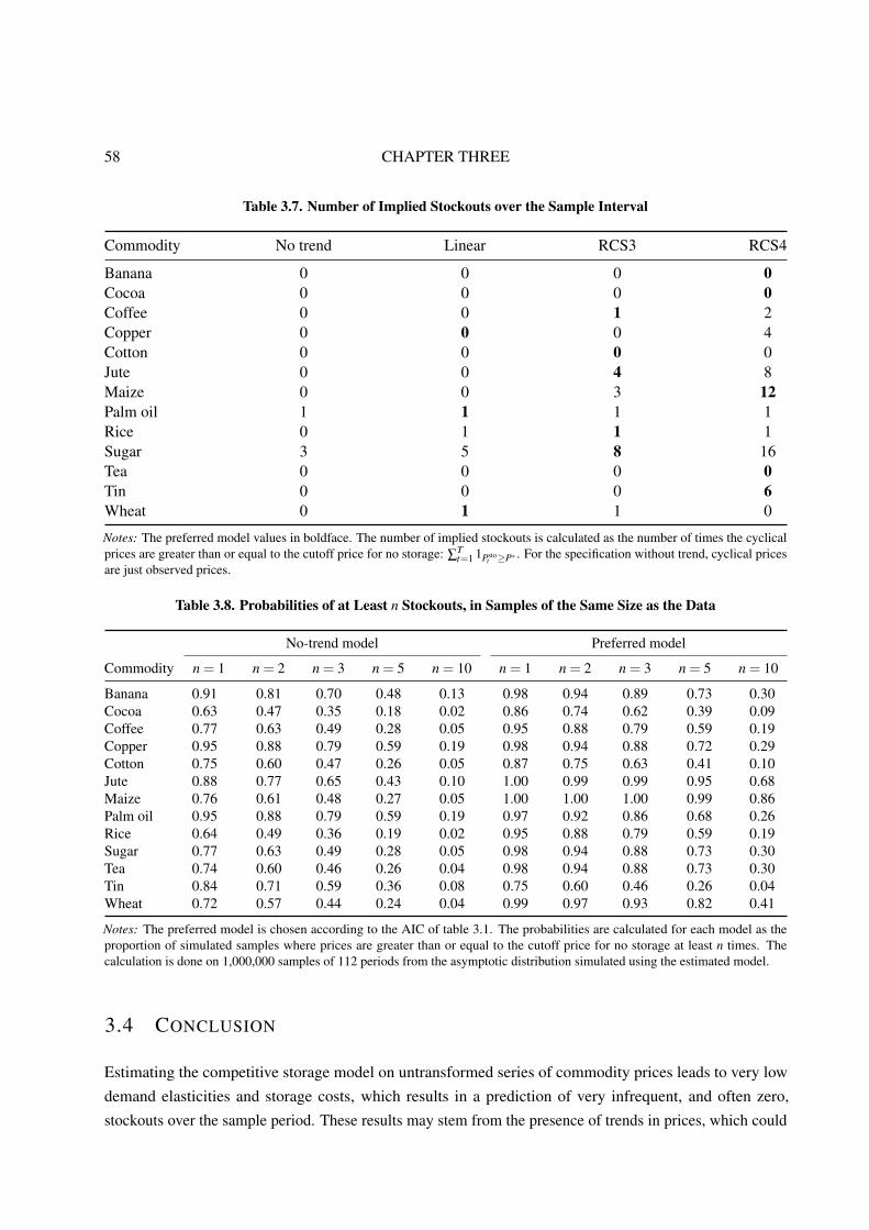
58 CHAPTER THREE
Table 3.7. Number of Implied Stockouts over the Sample Interval
Commodity No trend Linear RCS3 RCS4
Banana 0 0 0 0Cocoa 0 0 0 0Coffee 0 0 1 2Copper 0 0 0 4Cotton 0 0 0 0Jute 0 0 4 8Maize 0 0 3 12Palm oil 1 1 1 1Rice 0 1 1 1Sugar 3 5 8 16Tea 0 0 0 0Tin 0 0 0 6Wheat 0 1 1 0
Notes: The preferred model values in boldface. The number of implied stockouts is calculated as the number of times the cyclicalprices are greater than or equal to the cutoff price for no storage: ∑
Tt=1 1Psto
t ≥P∗ . For the specification without trend, cyclical pricesare just observed prices.
Table 3.8. Probabilities of at Least n Stockouts, in Samples of the Same Size as the Data
No-trend model Preferred model
Commodity n = 1 n = 2 n = 3 n = 5 n = 10 n = 1 n = 2 n = 3 n = 5 n = 10
Banana 0.91 0.81 0.70 0.48 0.13 0.98 0.94 0.89 0.73 0.30Cocoa 0.63 0.47 0.35 0.18 0.02 0.86 0.74 0.62 0.39 0.09Coffee 0.77 0.63 0.49 0.28 0.05 0.95 0.88 0.79 0.59 0.19Copper 0.95 0.88 0.79 0.59 0.19 0.98 0.94 0.88 0.72 0.29Cotton 0.75 0.60 0.47 0.26 0.05 0.87 0.75 0.63 0.41 0.10Jute 0.88 0.77 0.65 0.43 0.10 1.00 0.99 0.99 0.95 0.68Maize 0.76 0.61 0.48 0.27 0.05 1.00 1.00 1.00 0.99 0.86Palm oil 0.95 0.88 0.79 0.59 0.19 0.97 0.92 0.86 0.68 0.26Rice 0.64 0.49 0.36 0.19 0.02 0.95 0.88 0.79 0.59 0.19Sugar 0.77 0.63 0.49 0.28 0.05 0.98 0.94 0.88 0.73 0.30Tea 0.74 0.60 0.46 0.26 0.04 0.98 0.94 0.88 0.73 0.30Tin 0.84 0.71 0.59 0.36 0.08 0.75 0.60 0.46 0.26 0.04Wheat 0.72 0.57 0.44 0.24 0.04 0.99 0.97 0.93 0.82 0.41
Notes: The preferred model is chosen according to the AIC of table 3.1. The probabilities are calculated for each model as theproportion of simulated samples where prices are greater than or equal to the cutoff price for no storage at least n times. Thecalculation is done on 1,000,000 samples of 112 periods from the asymptotic distribution simulated using the estimated model.
3.4 CONCLUSION
Estimating the competitive storage model on untransformed series of commodity prices leads to very low
demand elasticities and storage costs, which results in a prediction of very infrequent, and often zero,
stockouts over the sample period. These results may stem from the presence of trends in prices, which could
TRENDING COMMODITY PRICES 59
create statistical features difficult to explain by a storage model.
This chapter proposes a strategy inspired by Canova (2014) to estimate jointly the structural parameters
of a storage model and the parameters characterizing the non-cyclical component of prices for which the
storage model cannot account. For the non-cyclical component of prices, three deterministic time trends with
increasing flexibility were tested and compared with the baseline model which ignores the possibility of a
trend.
Our results show that storage models with trend are always preferred to models without trend, and
the significance of the trend parameters indicates that the model without trend is likely to be misspecified.
Accounting for a trend is quantitatively important for estimating the structural parameters. For most
commodities, the storage model with a deterministic trend yields more plausible estimates of the structural
parameters (e.g., higher storage costs and demand elasticities). It also increases the probability of observing
stockouts, and more closely replicates the most salient features of the price data. For most commodities
our results support the empirical relevance of the speculative storage model which is in line with the recent
findings in Cafiero et al. (2011b, 2015) and prove that the joint estimation approach is a superior procedure
to fit the storage model with the data. Future estimations of the storage model should no longer neglect the
possibility of long-run trends in prices.
For banana, jute and tea, three of the commodities originally studied in Deaton and Laroque (1992), the
storage model with or without a deterministic trend fails to reproduce the main features of the price dynamics.
With the trend specifications considered in this chapter, the storage model is rejected as a relevant model to
explain the price dynamics of these commodities. However, other specifications could be explored in the
future.
This work is a first step toward jointly analyzing short- and long-run aspects of commodity prices. Our
focus was to show the importance of accounting for long-run trends when estimating the storage model, so
we have purposefully chosen simple deterministic trends that maintain the tractability of the likelihood, but
more sophisticated trend specifications could permit the reconciliation of two branches of the literature that
have long been separated. Because commodity prices are characterized by “small trends and big variability”
(Cashin and McDermott, 2002), without good explanations for the big short-run variability it is challenging
to identify the trends. Conversely, neglecting trends, even small ones, creates difficulties to explain the
short-run variability. To really integrate these two issues, several challenges will have to be faced. A storage
model in which agents account for trends implies theoretical restrictions such as an isoelastic demand
function that create numerical difficulties for the solution method. More sophisticated trends specifications
such as random walk with drift or log-linear trend with Markov switching slope would prevent a direct
calculation of the likelihood and would require the use of filters for non-linear state-space models (see e.g.,
Fernández-Villaverde and Rubio-Ramírez, 2007, for use of the particle filter to estimate macroeconomic
models). Some of the pieces are already provided in Zeng (2012), with a storage model including a structural
log-linear trend in prices, and Dvir and Rogoff (2014), with a storage model including a trend for quantities
following a random walk with drift, but further elaborations are needed to reach the level of sophistication
achieved in the literature on trends (Ghoshray, 2011).
60 CHAPTER THREE
3.A NUMERICAL METHOD
There is no closed-form solution for the equilibrium price function, which has to be approximated numerically.
The numerical method follows the fixed-point approach proposed by Deaton and Laroque (1992). The
equilibrium price function is approximated with a cubic spline over a grid of equally spaced availability
points lying between −2 and 20. The expectation term in equation (3.5) is replaced by a sum by discretizing
the truncated normal distribution of the production shocks ε using a Gaussian quadrature calculated by the
method of moments, with N = 10 nodes, where the production shocks and their associated probabilities are
denoted εn and πn. Then, using that production shocks are i.i.d., and combining (3.5) and (3.6) we have
P (A) = max
[β
N
∑n=1
πnP (A−D(P (A))+ ε
n)− k,D−1 (A)
]. (3.20)
The model is solved by iterating on this functional equation. Starting from a first guess for the price function,
a price function applied on the right-hand side to all grid points leads by simple arithmetic operations to new
values of the price function at the grid points on the left-hand side. The iterations stop when the Euclidean
distance between two consecutive price functions at the interpolating nodes falls below a given tolerance
threshold which we set to 10 decimal places.
Cafiero et al. (2011b) show that the estimation procedure is very sensitive to the accuracy of the model’s
numerical solution, which is determined mainly by the number of grid points used to approximate the policy
function P (A). These authors show that Deaton and Laroque (1996) approximate the policy function on
a grid that is too sparse to locate accurately the kink at the cutoff price P∗ of empty stocks, which partly
explains the inability of the storage model to generate the high serial correlation. Using a finer grid of 1,000
nodes, Cafiero et al. (2011b) obtain estimations of the parameters for which the storage model induces higher
price autocorrelations. We retain their findings and choose a grid of 1,000 points.
3.B COMPUTATIONAL DETAILS
The results were obtained using MATLAB R2014a on a PC with two quad-core processors Intel Xeon E5345
(2.33 GHz) with 32 GB of RAM running Ubuntu 12.04.5 64 bits. The maximization of the log-likelihood was
done using Vaz and Vicente’s (2007) free particle swarm pattern search software PSwarm version 2.114 and
the MATLAB function fmincon available in MATLAB Optimization Toolbox. The Monte-Carlo simulations
have been performed using MATLAB’s default random number generator with the seed set to 1. The
Gaussian quadrature was calculated using a MATLAB’s function from John Burkardt’s website.15 For a
unit normal distribution truncated at five standard deviations, the Gaussian quadrature with 10 nodes has
nodes εn = {±4.4576,±3.3999,±2.3838,±1.4132,±0.4684} and weights πn = {1.9834×10−5,1.2876×10−3,2.3048×10−2,0.14029,0.33536}.
14 http://www.mat.uc.pt/~lnv15 http://people.sc.fsu.edu/~jburkardt/m_src/truncated_normal_rule/truncated_normal_rule.html
TRENDING COMMODITY PRICES 61
3.C SMALL SAMPLE PROPERTIES
In this section, we assess using Monte Carlo experiments the small sample properties of the simulated
Unconditional Maximum Likelihood estimator (UML) we developed, and compare them to those of the
Conditional Maximum Likelihood estimator (CML) proposed in Cafiero et al. (2015). From equation (3.19),
the conditional log-likelihood without trend is obtained by removing the terms corresponding to the marginal
likelihood:
logLC (θ ;Pobs
1:T)=−T −1
2log2π− (T −1) log [Φ(5)−Φ(−5)]
+T
∑t=2
log∣∣∣P−1′ (Pobs
t)∣∣∣− T
∑t=2
(1|εt |≤5 · ε2
t +1|εt |>5 ·∞)/
2. (3.21)
Following Michaelides and Ng (2000) and Cafiero et al. (2015), we conduct four Monte Carlo experiments
varying the parameterization and the length of the samples. The first set of parameters are a = 1, b =−1,
and k = 0.02, which implies a storage cost of 2% of the mean price and, for supply shocks with a coefficient
of variation of 5%, a demand elasticity of −0.05 in the range of the best estimates obtained by Roberts
and Schlenker (2013) on a caloric aggregate of major crops, but slightly higher in absolute value than our
estimated elasticities. The second parameterization only differs by the value of b, now equal to −2. This
rotation of the slope of the demand function around its mean halves the demand elasticity making this
parameterization more favorable to storage, and closer to the values found in the chapter. For each set of
parameters, we solve for the equilibrium price function on a grid of 1,000 points, and obtain 3,000 prices
series of length T = 50 and T = 100 from the asymptotic distribution. The price series are obtained by the
simulation of 3,000 trajectories starting from the steady-state availability and discarding the first 50 periods
as burn-in periods.
The numerical methods follow what was described previously, but differ on two aspects. Firstly, to prevent
the availability corresponding to the cutoff price to be below the lower bound of the grid of interpolation
points, the lower bound is changed from being −2 to being −5, the minimum availability. Secondly, since
the log-likelihood optimization behaves better on simulated samples, we use a faster optimization algorithm:
the generalized pattern search algorithm implemented by the MATLAB function patternsearch available
in MATLAB Global Optimization Toolbox. The optimization starts from initial values randomly drawn in
the range between 80% and 120% of the true values. If the optimization solver fails to converge for one of
the two estimators, we discard the corresponding samples for both estimators. The results of valid estimates
obtained on common samples are given in table 3.9 and 3.10.
The results of the Monte Carlo experiments are similar to those obtained for the CML in Cafiero et al.
(2015). They show that the two maximum likelihood estimators yield precise estimates of the parameters of
the model, especially for a and b. The storage cost, k, is less precisely estimated with Root Mean Square
Errors (RMSE) always above 26%. For all parameters, the bias is small, most of the RMSE being explained
by the standard deviation of the estimations.
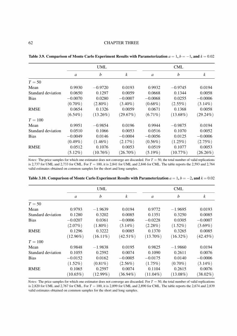
62 CHAPTER THREE
Table 3.9. Comparison of Monte Carlo Experiment Results with Parameterization a = 1, b =−1, and k = 0.02
UML CML
a b k a b k
T = 50Mean 0.9930 −0.9720 0.0193 0.9932 −0.9745 0.0194Standard deviation 0.0650 0.1297 0.0059 0.0668 0.1344 0.0058Bias −0.0070 0.0280 −0.0007 −0.0068 0.0255 −0.0006
(0.70%) (2.80%) (3.40%) (0.68%) (2.55%) (3.14%)RMSE 0.0654 0.1326 0.0059 0.0671 0.1368 0.0058
(6.54%) (13.26%) (29.67%) (6.71%) (13.68%) (29.24%)T = 100Mean 0.9951 −0.9854 0.0196 0.9944 −0.9875 0.0194Standard deviation 0.0510 0.1066 0.0053 0.0516 0.1070 0.0052Bias −0.0049 0.0146 −0.0004 −0.0056 0.0125 −0.0006
(0.49%) (1.46%) (2.17%) (0.56%) (1.25%) (2.75%)RMSE 0.0512 0.1076 0.0053 0.0519 0.1077 0.0053
(5.12%) (10.76%) (26.70%) (5.19%) (10.77%) (26.26%)
Notes: The price samples for which one estimator does not converge are discarded. For T = 50, the total number of valid replicationsis 2,737 for UML and 2,733 for CML. For T = 100, it is 2,841 for UML and 2,846 for CML. The table reports the 2,593 and 2,764valid estimates obtained on common samples for the short and long samples.
Table 3.10. Comparison of Monte Carlo Experiment Results with Parameterization a = 1, b =−2, and k = 0.02
UML CML
a b k a b k
T = 50Mean 0.9793 −1.9639 0.0194 0.9772 −1.9695 0.0193Standard deviation 0.1280 0.3202 0.0085 0.1351 0.3250 0.0085Bias −0.0207 0.0361 −0.0006 −0.0228 0.0305 −0.0007
(2.07%) (1.80%) (3.14%) (2.28%) (1.52%) (3.69%)RMSE 0.1296 0.3222 0.0085 0.1370 0.3265 0.0085
(12.96%) (16.11%) (42.51%) (13.70%) (16.32%) (42.45%)T = 100Mean 0.9848 −1.9838 0.0195 0.9825 −1.9860 0.0194Standard deviation 0.1055 0.2592 0.0074 0.1090 0.2611 0.0076Bias −0.0152 0.0162 −0.0005 −0.0175 0.0140 −0.0006
(1.52%) (0.81%) (2.56%) (1.75%) (0.70%) (3.14%)RMSE 0.1065 0.2597 0.0074 0.1104 0.2615 0.0076
(10.65%) (12.99%) (36.94%) (11.04%) (13.08%) (38.02%)
Notes: The price samples for which one estimator does not converge are discarded. For T = 50, the total number of valid replicationsis 2,820 for UML and 2,767 for CML. For T = 100, it is 2,899 for UML and 2,890 for CML. The table reports the 2,674 and 2,839valid estimates obtained on common samples for the short and long samples.
TRENDING COMMODITY PRICES 63
For all parameterizations, the estimators perform better when the sample length increases. For the
UML, a doubling of the sample length from 50 to 100 observations reduces the RMSE by 17% for both
parameterizations. The CML benefits slightly more than the UML from an increase in the sample size.
Indeed, they have similar RMSE for the long samples, but the UML performs better on the short samples.
Regarding the influence of the parameterization, we observe that the parameterization more favorable to
storage yields less precise estimates as all the RMSE of table 3.10 are higher than in table 3.9.
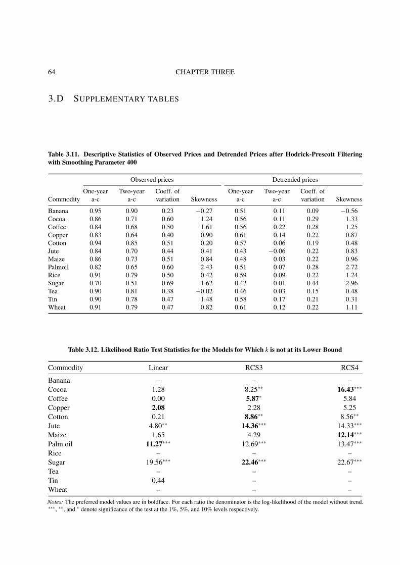
64 CHAPTER THREE
3.D SUPPLEMENTARY TABLES
Table 3.11. Descriptive Statistics of Observed Prices and Detrended Prices after Hodrick-Prescott Filteringwith Smoothing Parameter 400
Observed prices Detrended prices
One-year Two-year Coeff. of One-year Two-year Coeff. ofCommodity a-c a-c variation Skewness a-c a-c variation Skewness
Banana 0.95 0.90 0.23 −0.27 0.51 0.11 0.09 −0.56Cocoa 0.86 0.71 0.60 1.24 0.56 0.11 0.29 1.33Coffee 0.84 0.68 0.50 1.61 0.56 0.22 0.28 1.25Copper 0.83 0.64 0.40 0.90 0.61 0.14 0.22 0.87Cotton 0.94 0.85 0.51 0.20 0.57 0.06 0.19 0.48Jute 0.84 0.70 0.44 0.41 0.43 −0.06 0.22 0.83Maize 0.86 0.73 0.51 0.84 0.48 0.03 0.22 0.96Palmoil 0.82 0.65 0.60 2.43 0.51 0.07 0.28 2.72Rice 0.91 0.79 0.50 0.42 0.59 0.09 0.22 1.24Sugar 0.70 0.51 0.69 1.62 0.42 0.01 0.44 2.96Tea 0.90 0.81 0.38 −0.02 0.46 0.03 0.15 0.48Tin 0.90 0.78 0.47 1.48 0.58 0.17 0.21 0.31Wheat 0.91 0.79 0.47 0.82 0.61 0.12 0.22 1.11
Table 3.12. Likelihood Ratio Test Statistics for the Models for Which k is not at its Lower Bound
Commodity Linear RCS3 RCS4
Banana – – –Cocoa 1.28 8.25∗∗ 16.43∗∗∗Coffee 0.00 5.87∗ 5.84Copper 2.08 2.28 5.25Cotton 0.21 8.86∗∗ 8.56∗∗
Jute 4.80∗∗ 14.36∗∗∗ 14.33∗∗∗
Maize 1.65 4.29 12.14∗∗∗Palm oil 11.27∗∗∗ 12.69∗∗∗ 13.47∗∗∗
Rice – – –Sugar 19.56∗∗∗ 22.46∗∗∗ 22.67∗∗∗
Tea – – –Tin 0.44 – –Wheat – – –
Notes: The preferred model values are in boldface. For each ratio the denominator is the log-likelihood of the model without trend.∗∗∗, ∗∗, and ∗ denote significance of the test at the 1%, 5%, and 10% levels respectively.
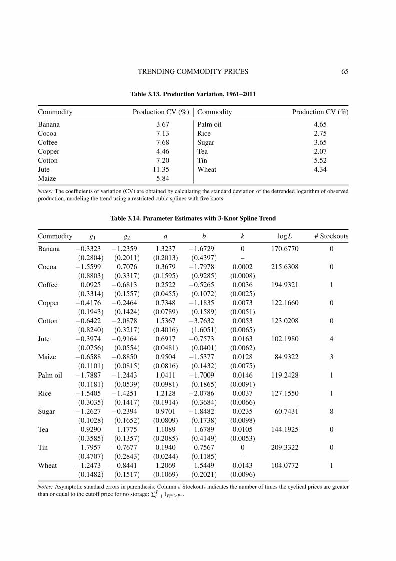
TRENDING COMMODITY PRICES 65
Table 3.13. Production Variation, 1961–2011
Commodity Production CV (%) Commodity Production CV (%)
Banana 3.67 Palm oil 4.65Cocoa 7.13 Rice 2.75Coffee 7.68 Sugar 3.65Copper 4.46 Tea 2.07Cotton 7.20 Tin 5.52Jute 11.35 Wheat 4.34Maize 5.84
Notes: The coefficients of variation (CV) are obtained by calculating the standard deviation of the detrended logarithm of observedproduction, modeling the trend using a restricted cubic splines with five knots.
Table 3.14. Parameter Estimates with 3-Knot Spline Trend
Commodity g1 g2 a b k logL # Stockouts
Banana −0.3323 −1.2359 1.3237 −1.6729 0 170.6770 0(0.2804) (0.2011) (0.2013) (0.4397) –
Cocoa −1.5599 0.7076 0.3679 −1.7978 0.0002 215.6308 0(0.8803) (0.3317) (0.1595) (0.9285) (0.0008)
Coffee 0.0925 −0.6813 0.2522 −0.5265 0.0036 194.9321 1(0.3314) (0.1557) (0.0455) (0.1072) (0.0025)
Copper −0.4176 −0.2464 0.7348 −1.1835 0.0073 122.1660 0(0.1943) (0.1424) (0.0789) (0.1589) (0.0051)
Cotton −0.6422 −2.0878 1.5367 −3.7632 0.0053 123.0208 0(0.8240) (0.3217) (0.4016) (1.6051) (0.0065)
Jute −0.3974 −0.9164 0.6917 −0.7573 0.0163 102.1980 4(0.0756) (0.0554) (0.0481) (0.0401) (0.0062)
Maize −0.6588 −0.8850 0.9504 −1.5377 0.0128 84.9322 3(0.1101) (0.0815) (0.0816) (0.1432) (0.0075)
Palm oil −1.7887 −1.2443 1.0411 −1.7009 0.0146 119.2428 1(0.1181) (0.0539) (0.0981) (0.1865) (0.0091)
Rice −1.5405 −1.4251 1.2128 −2.0786 0.0037 127.1550 1(0.3035) (0.1417) (0.1914) (0.3684) (0.0066)
Sugar −1.2627 −0.2394 0.9701 −1.8482 0.0235 60.7431 8(0.1028) (0.1652) (0.0809) (0.1738) (0.0098)
Tea −0.9290 −1.1775 1.1089 −1.6789 0.0105 144.1925 0(0.3585) (0.1357) (0.2085) (0.4149) (0.0053)
Tin 1.7957 −0.7677 0.1940 −0.7567 0 209.3322 0(0.4707) (0.2843) (0.0244) (0.1185) –
Wheat −1.2473 −0.8441 1.2069 −1.5449 0.0143 104.0772 1(0.1482) (0.1517) (0.1069) (0.2021) (0.0096)
Notes: Asymptotic standard errors in parenthesis. Column # Stockouts indicates the number of times the cyclical prices are greaterthan or equal to the cutoff price for no storage: ∑
Tt=1 1Psto
t ≥P∗ .

66 CHAPTER THREE
Table 3.15. Parameter Estimates with 4-Knot Spline Trend
Commodity g1 g2 g3 a b k logL # Stockouts
Banana −0.5940 −0.2663 −1.5903 1.2033 −1.5061 0 171.7633 0(0.2995) (0.3033) (0.2712) (0.1735) (0.3602) –
Cocoa 0.2862 −2.6193 0.3417 0.4498 −1.1874 0.0024 219.7236 0(0.2857) (0.5337) (0.4282) (0.0981) (0.2765) (0.0028)
Coffee 0.1199 0.0281 −0.7565 0.2339 −0.4885 0.0033 194.9185 2(0.1792) (0.3230) (0.1351) (0.0495) (0.0898) (0.0024)
Copper 0.6214 −0.8595 −0.2444 0.7416 −1.7526 0.0005 123.6516 4(0.3452) (0.3155) (0.1968) (0.1155) (0.3542) (0.0044)
Cotton −0.2545 −1.1035 −2.2689 1.4300 −3.5214 0.0049 122.8690 0(0.7621) (0.8597) (0.4857) (0.5264) (2.0232) (0.0069)
Jute −0.0613 −0.6035 −0.9908 0.6967 −0.7614 0.0163 102.1845 8(0.1039) (0.1805) (0.0710) (0.0797) (0.0715) (0.0066)
Maize 0.0815 −1.1899 −1.1229 0.9358 −0.8819 0.0304 88.8597 12(0.1073) (0.0887) (0.0576) (0.0481) (0.0508) (0.0068)
Palm oil −0.9208 −1.6398 −1.5053 0.9971 −1.6352 0.0142 119.6359 1(0.1402) (0.3924) (0.1190) (0.1744) (0.3267) (0.0095)
Rice −0.8285 −1.7697 −1.6808 1.2815 −2.2062 0.0042 127.1070 1(0.2131) (0.4977) (0.1837) (0.3139) (0.5310) (0.0070)
Sugar −0.6992 −1.3979 −0.3698 1.1136 −2.0999 0.0262 60.8484 16(0.1369) (0.2635) (0.2479) (0.1329) (0.2176) (0.0106)
Tea −1.4922 −0.4250 −1.8818 1.1959 −1.7916 0.0107 145.6865 0(0.3475) (0.4818) (0.2257) (0.2308) (0.4785) (0.0051)
Tin 1.7411 1.1081 −0.2441 0.1517 −0.5043 0 210.3823 6(0.5157) (0.2943) (0.1589) (0.0113) (0.0414) –
Wheat −0.1494 −1.9057 −0.9026 1.3447 −2.3618 0 105.8230 0(0.1744) (0.3087) (0.1902) (0.1606) (0.3405) –
Notes: Asymptotic standard errors in parenthesis. Column # Stockouts indicates the number of times the cyclical prices are greaterthan or equal to the cutoff price for no storage: ∑
Tt=1 1Psto
t ≥P∗ .

TRENDING COMMODITY PRICES 67
3.E SUPPLEMENTARY FIGURES
Banana Cocoa Coffee
Copper Cotton Jute
Maize Palm oil Rice
Sugar Tea Tin
Wheat
0.25
0.50
0.75
1.00
0.2
0.4
0.6
0.2
0.4
0.6
0.3
0.6
0.9
0.00
0.25
0.50
0.75
1.00
1.25
0.25
0.50
0.75
1.00
1.25
0.5
1.0
1.5
0.0
0.5
1.0
1.5
2.0
0.25
0.50
0.75
1.00
1.25
0.5
1.0
1.5
2.0
0.2
0.4
0.6
0.8
0.1
0.2
0.3
0.4
0.5
0.4
0.8
1.2
1.6
1920 1950 1980 2010Year
Pric
es
Real price Linear trend 3−knot spline trend 4−knot spline trend
Figure 3.4. Price trends
CHAPTER 4
BAYESIAN ESTIMATION OF THE STORAGE MODEL USING
INFORMATION ON QUANTITIES
In research on commodity prices behavior’s, the rational expectations storage model of Gustafson (1958)
has become the workhorse model for prices formation and commodity market volatility studies. In the model,
the dynamics of commodity prices is explained by real shocks to supply and demand influencing the decisions
made by optimizing forward-looking agents. Although the theoretical foundations of the storage model
are well grounded, its empirical validity continues to be challenged. In pathbreaking papers, Deaton and
Laroque (1992, 1996) cast doubt on its relevance because of its inability to generate the observed high levels
of autocorrelation in prices. This serial correlation puzzle has been partially solved in part through several
refinements to improve the accuracy of the numerical methods (Cafiero et al., 2011b), the development of a
Maximum Likelihood estimator (Cafiero et al., 2015), the choice of the data used (Guerra et al., 2015), and
management of the trend (Gouel and Legrand, 2016b). However, all these previous estimations are based
only on prices information, and ignore the data on quantities, although these would introduce some noise.
Another problem with price-only estimations is that many parameters, such as those related to the supply
process, are left unidentified. So these estimations have to assume an inelastic supply which is modeled by a
unit normal random shock.
In this chapter, we develop a new econometric approach to the storage model estimation that is able to
use observables other than prices by borrowing from the recent literature on the estimation of DSGE models.
This new approach allows us to estimate a richer storage model than the specifications previously estimated.
For example, our storage model features two structural shocks to supply and demand, instead of only one to
supply, and includes producers that react to expected price changes. Now that the literature has showed that
the storage model is able to fit price dynamics, it is important to assess whether it is able to do so while also
accommodating quantities behavior.
In the standard storage model, when observables other than prices are added, the model presents a
stochastic singularity. With only one shock in the model, the combination of observables would not be
consistent with the theory leading to a likelihood that would be zero with probability one. To avoid this
Chapter written with Christophe Gouel.
BAYESIAN ESTIMATION OF THE STORAGE MODEL USING INFORMATION ON QUANTITIES69
problem, we follow the literature on the estimation of DSGE models by adding structural and measurement
shocks (Fernández-Villaverde, 2010). Adding shocks of measurement errors may have important conse-
quences for the estimation procedure. These additional shocks may make impossible to recover the state of
the model from the observables and so to calculate the likelihood analytically. This situation would call for
nonlinear filtering techniques, known as particle filtering. In this preliminary version of the study, we focus
on cases such that measurement errors do not prevent the observation of the state, which allows us to have
likelihood functions that take analytic form. Because of this restriction, we have to assume that prices are
always observed without noise so that a one-to-one mapping exists between prices and market availability.
Only consumption and production are assumed to be observed with noise. Depending on the number of
structural shocks and observed variables used, we estimate a sequence of model specifications allowing
us to analyze how information from consumption and production contributes to parameters’ identification.
Our most simple specification, with prices as the only observables, leads to the same likelihood function as
Cafiero et al. (2015). Starting from Cafiero et al. approach, we build more general likelihood functions in
order to accommodate the additional observables. As for other rational expectations models, the likelihood
functions are challenging to maximize and we estimate the model using Bayesian methods.
Because this is a new approach to estimating the storage model, we carry the estimations on a sample for
which we have good benchmark estimations to which our work can be compared: the global markets for
calories coming from maize, rice, soybeans, and wheat from 1961 to 2006. Roberts and Schlenker (2013) use
the storage model to motivate the choice of instrumental variables for reduced-form estimations of supply
and demand on this market for calories. Aggregating staple foods into calories allows to account for about
75% percent of the global food production and to bypass many issues related to the close substituability in
production and consumption of these major crops, such as the risks of mixing own-price with cross-price
elasticities. Even if our elasticities tend to be slightly lower, overall our results are consistent with Roberts
and Schlenker’s results. Our estimations also predict some stockouts over the estimation sample (2 to 5
depending on the specification), consistent with the rare price spikes observed in the sample.
The remainder of the chapter is organized as follows. Section 4.1 describes the storage model and the
solution method. Section 4.2 presents our data and some descriptive statistics. Section 4.3 presents the
Bayesian estimation strategy, the chosen priors, and the model’s posterior. Section 4.4 concludes.
4.1 THE MODEL
4.1.1 MODEL EQUATIONS
Let consider a model of the world market for a storable staple (here the caloric aggregate of maize, rice,
soybeans, and wheat). The storage model is based on Wright and Williams (1982) and is a partial equilibrium
model featuring profit-maximizing producers, competitive storers with constant marginal storage costs which
can transfer the good across time, and a demand function. We extend Wright and Williams’ model to make
it consistent with a balanced growth path driven by a deterministic increase in demand and a reduction in
marginal production costs.
70 CHAPTER FOUR
There are a few differences with respect to the storage models used for previous structural estimations
(Deaton and Laroque, 1992, 1996, Cafiero et al., 2011b, 2015). First, in our case supply is elastic to prices
while previous models tell us nothing about the agricultural producers’ reactions to prices: producers are
not represented explicitly and production consists only of an exogenous supply shock. Second, we add
another structural shock to demand. Most storage models feature only one structural shock, usually a supply
shock, which in fact can be interpreted as a net supply shock. When using information on consumption and
production for the estimation, it is useful to have structural shocks corresponding to each observable. To
avoid making the numerical method more complex, we assume that demand and supply shocks are additive,
which allows us to sum shocks, available stocks and planned production, leading to a model with only one
state variable.
PRODUCERS A representative producer makes its production decision and pays for inputs one period before
bringing its output to the market. The production choice, made in period t, is denoted Q̃t . Realized production
differ from planned production by an exogenous additive shock, η̃Qt+1, occurring during the growing season
(e.g., a weather disturbance). The producer’s problem in period t can be written as
maxQ̃t
(1+ r)−1 Et Pt+1
(Q̃t + η̃
Qt+1
)− Ψ̃t
(Q̃t), (4.1)
where r is the real interest rate which is assumed to be fixed, Et is the expectation operator conditional on
period t information, Pt+1 is the price, and Ψ̃t (·) is a differentiable and convex production cost function. The
solution to this problem is the following first-order condition
(1+ r)−1 Et Pt+1 = Ψ̃′t(Q̃t). (4.2)
At each period, the producer rationally plants up to the point where the expected marginal benefit equals the
marginal production cost.
STORERS Competitive storers are risk-neutral. For storing an amount S̃t ≥ 0 from period t until t +1 they
incur a physical cost of storage proportional to the stored quantities, kS̃t , and an opportunity cost. Assuming
rational expectations and taking account of the non-negativity constraint on storage yield the following
arbitrage condition
(1+ r)−1 Et Pt+1−Pt − k ≤ 0, = 0 if S̃t > 0. (4.3)
FINAL DEMAND Final demand for the good is the sum of a downward sloping demand function D̃t (Pt) and
a demand shock denoted η̃Dt .
EQUILIBRIUM The market clears when previous stocks plus production equal final demand plus demand
for stocks:
S̃t−1 + Q̃t−1 + η̃Qt = D̃t (Pt)+ η̃
Dt + S̃t . (4.4)
BAYESIAN ESTIMATION OF THE STORAGE MODEL USING INFORMATION ON QUANTITIES71
TRENDS AND STEADY-STATE GROWTH Consumption and production of food grow steadily over time
because of population increase, income growth, or technological progress. To account for this fact, we
allow the demand function, the marginal cost function, and the structural shocks to have deterministic trends.
Because of the additivity of the market clearing equation, to obtain steady-state growth requires the adoption
of multiplicative trends. Detrended variables are expressed without “tilde” and related to their trending
counterparts by the following relations
D̃t (Pt) = (1+g)t D(Pt) , (4.5)
Ψ̃′t(Q̃t)= Ψ
′ (Qt) , (4.6)
η̃Qt = (1+g)t
ηQt , (4.7)
η̃Dt = (1+g)t
ηDt , (4.8)
where g is the assumed growth rate. Equation (4.6) imposes that the downward trend in marginal production
costs perfectly offsets the trend in production, leaving prices stationary. Because of the additive nature of
equation (4.3) determining the storage level, to be compatible with a steady-state growth any trend in prices
will require marginal storage costs, k, either to be zero or to have the same trend as prices, two restrictions
which are unlikely to hold. To avoid imposing these restrictions, we ignore potential trends in prices.1 This set
of trend assumptions induces a common multiplicative trend in all quantities: final consumption, production
and stocks. Using the convention S̃t = St (1+g)t and Q̃t−1 = Qt−1 (1+g)t , replacing trending quantities by
their detrended counterparts in the market clearing equation leads to
St−1
1+g+Qt−1 +η
Qt = D(Pt)+η
Dt +St . (4.9)
The division of St−1 by 1+ g illustrates that, on average, stocks have to increase just to meet the pace of
increase in production and demand, so detrended beginning stocks are discounted by 1+g to maintain them
at a level comparable to other detrended quantities.
STATIONARY EQUILIBRIUM In equation (4.9), four variables are predetermined: stocks, planned production
and the two shocks. They can be summed together in a single state variable, availability net of demand shock
At :
At ≡St−1
1+g+Qt−1 +η
Qt −η
Dt . (4.10)
The capacity to combine all predetermined variables in one state variable is crucial to simplify numerical
resolution of the model and this simplification is allowed by assuming an additive demand shock.
Equation (4.10) is the model’s stationary transition equation. Applying previous transformations to the
1 See Dvir and Rogoff (2014) for another storage model with trending quantities but without trending prices.
72 CHAPTER FOUR
equilibrium equations leads to the following three stationary equilibrium equations:
(1+ r)−1 Et Pt+1 = Ψ′(Qt) , (4.11)
(1+ r)−1 Et Pt+1−Pt − k ≤ 0, = 0 if St > 0, (4.12)
At = St +D(Pt) . (4.13)
We assume that the stationary demand function takes the following linear form
D(Pt) = D̄(
1+αD Pt − P̄
P̄
), (4.14)
where D̄ is the steady-state demand (equal also to steady-state production since stocks are not held at the
steady state), αD < 0 is the price elasticity of demand at the steady state, and P̄ is the steady-state price.
Similarly, the stationary marginal cost function is assumed to be linear:
Ψ′ (Qt) = (1+ r)−1 P̄
(1+
1αS
Qt − D̄D̄
), (4.15)
where αS > 0 is the supply elasticity at the steady state. Because of the assumed specifications in deviation
from the deterministic steady state, these demand and marginal cost functions depend only on parameters
that can be directly interpreted, which is important for the prior elicitation of the Bayesian analysis.
ηQt and ηD
t , the stationary supply and demand disturbances, are assumed to be serially uncorrelated,
independent of each other, and are normally distributed with zero mean and standard deviations σηQ and σηD .
We also estimate a version of the model with inelastic supply. In this case, equation (4.11) is dropped
from the model and planned production is fixed at its steady-state level: Qt = D̄. Except for the demand
shock and the growth rate g, this version of the storage model is the same as the one estimated in Deaton and
Laroque (1992).
4.1.2 MODEL SOLUTION
Equations (4.10)–(4.13) form a non-linear rational expectations system based on the variables At , Qt , St , and
Pt driven by the innovations ηt =[η
Qt ,ηD
t
]. This system does not have a closed form solution and must be
solved numerically to allow for a structural estimation. Solution of the rational expectations system takes the
form of policy functions which describe control variables as functions of the contemporaneous state variable,
net availability:
Qt = Q (At) , (4.16)
St = S (At) , (4.17)
Pt = P (At) , (4.18)
to which the transition equation (4.10) must be added.
BAYESIAN ESTIMATION OF THE STORAGE MODEL USING INFORMATION ON QUANTITIES73
Combining equations (4.10) to (4.13), one can see that the policy functions for all At have to satisfy:
P (At) = max[(1+ r)−1 Et P
(S (At)+Q (At)+η
Qt+1−η
Dt+1
)− k,D−1 (At)
], (4.19)
(1+ r)−1 Et P(S (At)+Q (At)+η
Qt+1−η
Dt+1
)= Ψ
′ (Q (At)) . (4.20)
Equation (4.19) makes clear the existence of two regimes. The first regime holds when speculators stockpile
in the expectation of future prices covering the full carrying costs and the purchasing cost. The second regime
defines the stockout situation with empty inventories, where the market price is determined only by the final
demand for consumption and the net availability in the market. Let us define P∗ as the cutoff price above
which there is no storage. This cutoff price is the solution to the following nonlinear equation
P∗ = (1+ r)−1 Et P(Q (D(P∗))+η
Qt+1−η
Dt+1
)− k, (4.21)
which depends on the policy functions.
A variety of numerical techniques is available to solve rational expectations storage models and approxi-
mate the policy functions (Gouel, 2013a). Previous estimations of the storage model relied on the fixed-point
algorithm of Deaton and Laroque (1992). This has the advantage that it is very fast because it requires no
rootfinding operation. However, it does not apply to models with elastic supply. The numerical algorithm
we implement is the endogenous grid method proposed by Carroll (2006), adapted to the storage model in
Gouel (2013a). In the case of a model with inelastic supply, like Deaton and Laroque’s algorithm it implies
simple arithmetic operations only, but no rootfinding. With elastic supply, it is necessary to solve nonlinear
equations, but this algorithm is still much faster than the alternatives. One advantage over the approach in
Deaton and Laroque is that the endogenous grid method locates precisely the cutoff point of no storage even
with a small number of grid points, whereas the the fixed-point algorithm requires a large number of grid
points (Cafiero et al., 2011b).
To implement the algorithm, the expectations terms in equations (4.11) and (4.12) are replaced by sums
by discretizing the normal distribution of the net supply shocks ηQ−ηD using a Gauss-Hermite quadrature
with 11 nodes. We use a regular grid on storage of 50 nodes spanning the interval [0, D̄], where D̄ is fixed at
1, its central value in the estimations below. The algorithm stops when successive policy functions cease to
differ by more than a given tolerance threshold, set to 10 decimal places. See Gouel (2013a) for more details
on the implementation of the algorithm.
4.2 OVERVIEW OF THE GRAINS MARKET
4.2.1 DATA
The data on world quantities for maize, rice, soybeans and wheat come from the Food and Agriculture
Organization statistical database (FAOSTAT). Total demand is obtained by subtracting the variation in
inventories from total production. Our sample starts in 1961, the first year available in FAOSTAT. It ends

74 CHAPTER FOUR
in 2006 because, after that year, the increasing importance of biofuels, supported strongly by US and EU
policies, may have changed the behavior of the food markets (biofuel mandates create an additional inelastic
demand for food products, while biofuel demand induced by tax credits may link food and oil markets).2
Following the approach proposed by Roberts and Schlenker (2013), the four commodities are aggregated
together into calories using the conversion ratios in Williamson and Williamson (1942). Figure 4.1 depicts
the patterns of the world production and consumption over the sample period. Although production appears
more volatile than consumption, both production and consumption grow at the same steady linear rate over
time. We need stationary variables for the estimation. Production and consumption are regressed on the same
linear time trend. The residuals are centered on 2006 trend values and normalized to have unitary mean.
1960 1970 1980 1990 2000
2
3
4
5
6
7
Year
Bill
ion
peop
le (
2,00
0 ki
loca
lori
es p
er d
ay)
ProductionConsumptionTrend
Figure 4.1. World caloric production and consumption, and their trend for 1961–2006. The y-axis is the numberof people who hypothetically could be fed on a 2,000 kilocalories per day diet based on consuming only the fourcommodities.
Regarding prices, a crucial issue is deciding what is the most relevant annual price series to use to estimate
of the storage model. The series of prices used in Deaton and Laroque (1992) are formed by averaging prices
over the calendar year, which might induce spurious correlations due to mixing together different marketing
seasons. Guerra et al. (2015) compare the model fit for a storage model when estimated on different price
series for maize and find that the price for the first month following the delivery is what works best. Roberts
and Schlenker (2013) adopt the strategy of a single month per year, which is the approach used here. Nominal
2 See Wright (2014) and de Gorter et al. (2015) for more.
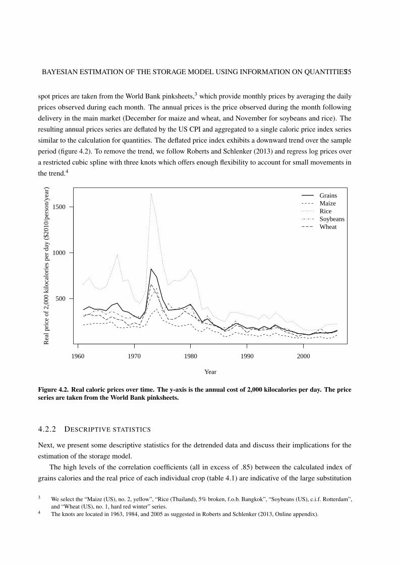
BAYESIAN ESTIMATION OF THE STORAGE MODEL USING INFORMATION ON QUANTITIES75
spot prices are taken from the World Bank pinksheets,3 which provide monthly prices by averaging the daily
prices observed during each month. The annual prices is the price observed during the month following
delivery in the main market (December for maize and wheat, and November for soybeans and rice). The
resulting annual prices series are deflated by the US CPI and aggregated to a single caloric price index series
similar to the calculation for quantities. The deflated price index exhibits a downward trend over the sample
period (figure 4.2). To remove the trend, we follow Roberts and Schlenker (2013) and regress log prices over
a restricted cubic spline with three knots which offers enough flexibility to account for small movements in
the trend.4
1960 1970 1980 1990 2000
500
1000
1500
Year
Rea
l pri
ce o
f 2,
000
kilo
calo
ries
per
day
($2
010/
pers
on/y
ear)
GrainsMaizeRiceSoybeansWheat
Figure 4.2. Real caloric prices over time. The y-axis is the annual cost of 2,000 kilocalories per day. The priceseries are taken from the World Bank pinksheets.
4.2.2 DESCRIPTIVE STATISTICS
Next, we present some descriptive statistics for the detrended data and discuss their implications for the
estimation of the storage model.
The high levels of the correlation coefficients (all in excess of .85) between the calculated index of
grains calories and the real price of each individual crop (table 4.1) are indicative of the large substitution
3 We select the “Maize (US), no. 2, yellow”, “Rice (Thailand), 5% broken, f.o.b. Bangkok”, “Soybeans (US), c.i.f. Rotterdam”,and “Wheat (US), no. 1, hard red winter” series.
4 The knots are located in 1963, 1984, and 2005 as suggested in Roberts and Schlenker (2013, Online appendix).
76 CHAPTER FOUR
possibilities between these crops. With the exceptions of soybeans and maize, the crops are correlated more
to the aggregate than to any other crop. This supports use of an aggregated caloric indicator as a suitable
measure of the state of the world food market. Estimation based on each crop individually would create the
risk of mixing own-price and cross-price elasticities.
Table 4.1. Correlation coefficients of detrended real prices data, 1961–2006
Commodity Grains Maize Rice Soybeans Wheat
Grains 1.000 0.897 0.972 0.856 0.950Maize 0.897 1.000 0.795 0.886 0.873Rice 0.972 0.795 1.000 0.774 0.875Soybeans 0.856 0.886 0.774 1.000 0.813Wheat 0.950 0.873 0.875 0.813 1.000
Notes: Prices are detrended using a restricted cubic splines using three knots. “Grains” refers to the caloric aggregate of maize, rice,soybeans, and wheat.
Table 4.2 reports the descriptive statistics of the data used to estimate the model. The first-order
autocorrelation of prices is high at 0.615. Higher values of autocorrelation (mostly above 0.8) were observed
on a different sample by Deaton and Laroque (1992), which led them to reject the storage model because of its
inability to match these high levels. Competitive storage behavior is able to explain positively autocorrelated
prices, but not very high levels. Hence, the importance of detrending the prices because the model is able to
explain only cyclical fluctuations not long-run trends (Gouel and Legrand, 2016b). Consumption also presents
a high serial correlation at 0.73, which is consistent with the fact that, except in the case of structural and
measurement shocks, consumption should follow price behavior. The first- and second-order autocorrelations
are higher for consumption than for price, likely explained by autocorrelated demand shocks. We do not
consider this possibility here, but it would make sense if demand shocks are not idiosyncratic but related
to the business cycle. Production presents a small first-order autocorrelation of 0.163. With respect to the
storage model, this small autocorrelation indicates that uncorrelated supply shocks are quantitatively more
important than endogenous supply reactions. The absence of autocorrelation in production supports the
relevance of storage to generate price persistence.
Table 4.2. Autocorrelation and coefficient of variation of detrended caloric data, 1961–2006
One-year Two-year CoefficientVariable a-c a-c of variation
Production 0.163 −0.098 0.021Consumption 0.730 0.418 0.011Price 0.615 0.181 0.298
The coefficients of variation of production and consumption are quite low at 2.1% and 1.1% respectively.
The fact that production is more volatile than consumption shows the importance of inter-annual storage.
Without storage, changes in production levels would have to be matched each year by corresponding changes

BAYESIAN ESTIMATION OF THE STORAGE MODEL USING INFORMATION ON QUANTITIES77
in consumption levels. Price is much more volatile than consumption. To reproduce this would require a very
inelastic demand curve.
Table 4.3 displays the correlation coefficients of production, consumption, and price. The correlations
have the expected signs, with a negative correlation between consumption and price and a positive one
between production and consumption. However, production and consumption are not perfectly correlated,
which again points to the role of storage. Because of storage, in the model, consumption is not determined by
production but by the sum of production and stocks. Therefore, production should affect consumption, but this
effect is mitigated by the presence of stocks. The low correlation between consumption and price indicates
that a lot of the movements observed for consumption stems not from movements along the demand curve,
but from movements in the demand curve itself or from measurement errors. If it was due only to movements
along the demand curve the correlation would be close to −1. This low correlation between consumption and
price exemplifies the standard econometric challenge in the estimation of demand elasticities: price variations
are caused by supply and demand shocks and movements along the supply and demand curves, with the
result that identification of a demand elasticity requires the price variations from exogenous supply shocks
to be isolated. Some works have propose clever empirical strategies aimed at isolating clear exogenous
supply shocks (Adjemian and Smith, 2012, Roberts and Schlenker, 2013). In this study, the identification
comes from the assumed structural form of the model, which allows to recover the various shocks from the
observations.
Table 4.3. Correlation coefficients of detrended caloric data, 1961–2006
Variable Production Consumption Price
Production 1.000 0.390 −0.122Consumption 0.390 1.000 −0.121Price −0.122 −0.121 1.000
4.3 ESTIMATION
In this section, we propose an econometric procedure to estimate the storage model using information on
quantities. Thus far, structural estimations of the storage model have been undertaken assuming that: (i)
supply is inelastic, (ii) only one shock, a supply shock, is generating prices dynamics, (iii) price is the only
observable, and (iv) prices are observed without measurement errors. Under these assumptions, Cafiero et al.
(2015) develop a Maximum Likelihood estimator. Starting from the same likelihood function, we gradually
relax these four assumptions to provide a more comprehensive picture of how production, consumption
and spot prices are connected by storage decisions. In this preliminary version of the work, we maintain
assumption (iv) that prices are observed without measurement errors. This assumption allows the likelihood
to take an analytic form.
Once evaluated, the likelihood function can either be maximized over a vector of parameters θ following
the frequentist approach, or according to Bayes’ theorem, can be combined with a prior distribution of the
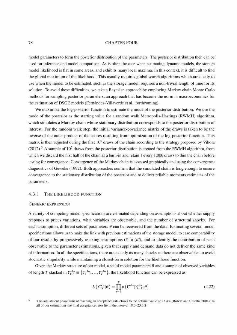
78 CHAPTER FOUR
model parameters to form the posterior distribution of the parameters. The posterior distribution then can be
used for inference and model comparison. As is often the case when estimating dynamic models, the storage
model likelihood is flat in some areas, and exhibits many local maxima. In this context, it is difficult to find
the global maximum of the likelihood. This usually requires global search algorithms which are costly to
use when the model to be estimated, such as the storage model, requires a non-trivial length of time for its
solution. To avoid these difficulties, we take a Bayesian approach by employing Markov chain Monte Carlo
methods for sampling posterior parameters, an approach that has become the norm in macroeconomics for
the estimation of DSGE models (Fernández-Villaverde et al., forthcoming).
We maximize the log-posterior function to estimate the mode of the posterior distribution. We use the
mode of the posterior as the starting value for a random walk Metropolis-Hastings (RWMH) algorithm,
which simulates a Markov chain whose stationary distribution corresponds to the posterior distribution of
interest. For the random walk step, the initial variance-covariance matrix of the draws is taken to be the
inverse of the outer product of the scores resulting from optimization of the log-posterior function. This
matrix is then adjusted during the first 105 draws of the chain according to the strategy proposed by Vihola
(2012).5 A sample of 107 draws from the posterior distribution is created from the RWMH algorithm, from
which we discard the first half of the chain as a burn-in and retain 1 every 1,000 draws to thin the chain before
testing for convergence. Convergence of the Markov chain is assessed graphically and using the convergence
diagnostics of Geweke (1992). Both approaches confirm that the simulated chain is long enough to ensure
convergence to the stationary distribution of the posterior and to deliver reliable moments estimates of the
parameters.
4.3.1 THE LIKELIHOOD FUNCTION
GENERIC EXPRESSION
A variety of competing model specifications are estimated depending on assumptions about whether supply
responds to prices variations, what variables are observable, and the number of structural shocks. For
each assumption, different sets of parameters θ can be recovered from the data. Estimating several model
specifications allows us to make the link with previous estimations of the storage model, to ease comparability
of our results by progressively relaxing assumptions (i) to (iii), and to identify the contribution of each
observable to the parameter estimations, given that supply and demand data do not deliver the same kind
of information. In all the specifications, there are exactly as many shocks as there are observables to avoid
stochastic singularity while maintaining a closed-form solution for the likelihood function.
Given the Markov structure of our model, a set of model parameters θ and a sample of observed variables
of length T stacked in Y obs1:T ≡
{Y obs
1 , . . . ,Y obsT}
, the likelihood function can be expressed as
L(Y obs
1:T |θ)=
T
∏t=1
p(Y obs
t |Y obst−1;θ
). (4.22)
5 This adjustment phase aims at reaching an acceptance rate closes to the optimal value of 23.4% (Robert and Casella, 2004). Inall of our estimations the final acceptance rates lie in the interval 18.3–23.3%.

BAYESIAN ESTIMATION OF THE STORAGE MODEL USING INFORMATION ON QUANTITIES79
Assumptions about structural measurement error shocks are made such that there are as many shocks as
there are observables and such that the method of variable transformation can be applied. In this case, the
conditional density of Y obst can be written as
p(Y obs
t |Y obst−1;θ
)= p(Vt) |Jt | , (4.23)
where Vt is a vector of the error terms which include structural and measurement error shocks, and |Jt | is the
determinant of the Jacobian of the mapping of Y obst 7→Vt .
Under the assumption of centered normally distributed shocks, p(Vt) is the density of a multivariate
normal and the likelihood function of the state-space model takes the following general form:
L(Y obs
1:T |θ)= (2π)−
nT2
T
∏t=1|Σ|−1/2 exp
(−V ′t Σ−1Vt
2
)|Jt | , (4.24)
where n is the number of observed variables stacked in Y obs and Σ is the variance-covariance matrix of V .
A specific model is defined by its vector of error terms Vt which in turn, determines Σ and Jt . Given these
three elements we can define the likelihood function.
MODEL-SPECIFIC LIKELIHOOD FUNCTION
In the remainder of the chapter, a model is denoted by letters and numbers respectively indicating the
observables and the number of assumed structural shocks. For instance for the model PQ1, the observables
are price and production, and there is one structural shock, a supply shock. For PDQ2, the observables are
price, consumption, and production, and there are two structural shocks, supply and demand shocks.
For brevity, we demonstrate how to evaluate the likelihood function only for the two most comprehensive
specifications with elastic supply and for which the vector of observed variables Y obs =(Pobs,Dobs,Qobs
)′includes price, consumption, and production. These specifications nest the others.6
MODEL PDQ1 Let consider that prices fluctuations are driven solely by unexpected supply disturbances ηQ
(i.e., ηD = 0). In contrast to consumption and production, prices are assumed to be observed without noise.
So the vector of errors is Vt =(
ηQt ,εD
t ,εQt
)′, where εD and εQ are measurement errors on consumption and
production. Following Cafiero et al. (2015), a production shock can be recovered from observation of two
consecutive prices using equation (4.10). So the various elements of Vt are defined by
ηQt = P−1 (Pobs
t)−S
(P−1
(Pobs
t−1
))1+g
−Q(P−1 (Pobs
t−1))
, (4.25)
εDt = Dobs
t −D(Pobs
t), (4.26)
εQt = Qobs
t −Q(P−1 (Pobs
t−1))−η
Qt = Qobs
t −P−1 (Pobst)+
S(P−1
(Pobs
t−1
))1+g
. (4.27)
6 The other set-up are available upon request.
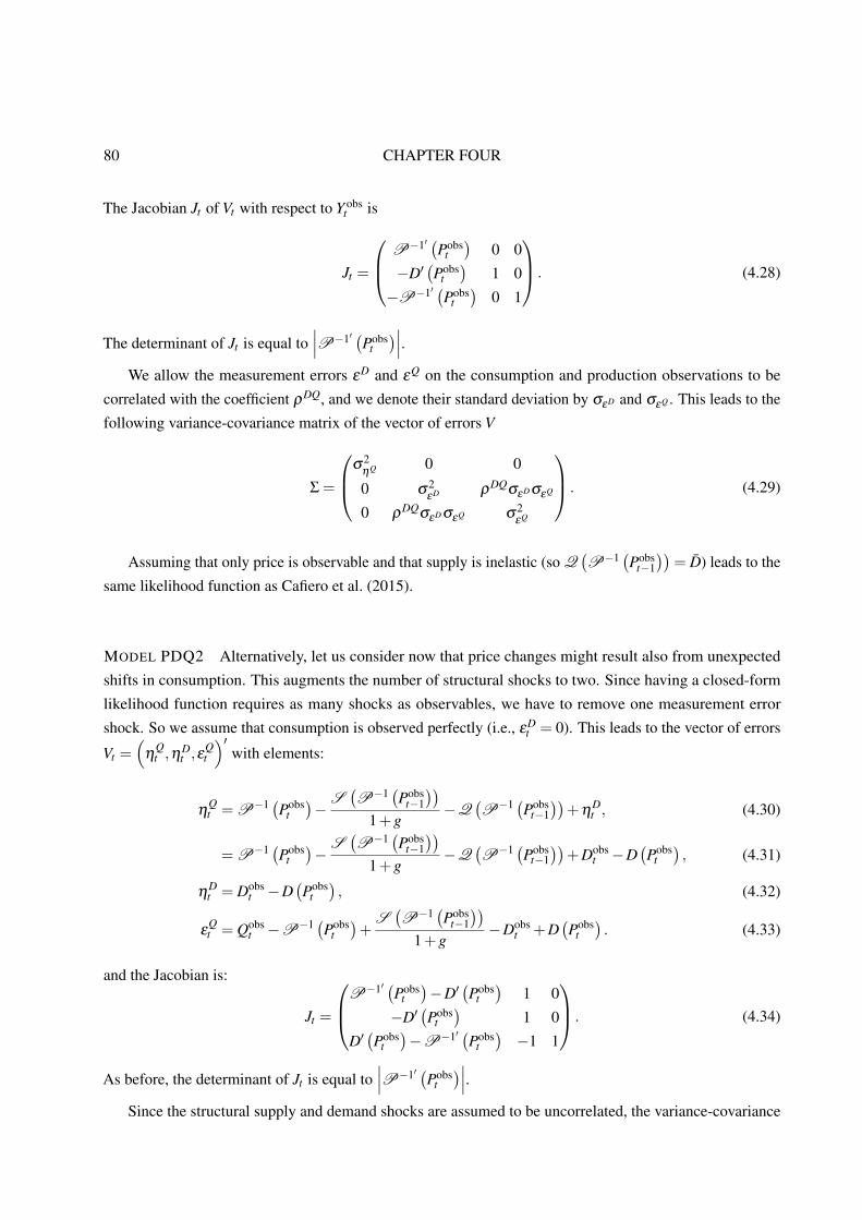
80 CHAPTER FOUR
The Jacobian Jt of Vt with respect to Y obst is
Jt =
P−1′(Pobs
t)
0 0
−D′(Pobs
t)
1 0
−P−1′(Pobs
t)
0 1
. (4.28)
The determinant of Jt is equal to∣∣∣P−1′
(Pobs
t)∣∣∣.
We allow the measurement errors εD and εQ on the consumption and production observations to be
correlated with the coefficient ρDQ, and we denote their standard deviation by σεD and σεQ . This leads to the
following variance-covariance matrix of the vector of errors V
Σ =
σ2ηQ 0 0
0 σ2εD ρDQσεDσεQ
0 ρDQσεDσεQ σ2εQ
. (4.29)
Assuming that only price is observable and that supply is inelastic (so Q(P−1
(Pobs
t−1
))= D̄) leads to the
same likelihood function as Cafiero et al. (2015).
MODEL PDQ2 Alternatively, let us consider now that price changes might result also from unexpected
shifts in consumption. This augments the number of structural shocks to two. Since having a closed-form
likelihood function requires as many shocks as observables, we have to remove one measurement error
shock. So we assume that consumption is observed perfectly (i.e., εDt = 0). This leads to the vector of errors
Vt =(
ηQt ,ηD
t ,εQt
)′with elements:
ηQt = P−1 (Pobs
t)−S
(P−1
(Pobs
t−1
))1+g
−Q(P−1 (Pobs
t−1))
+ηDt , (4.30)
= P−1 (Pobst)−S
(P−1
(Pobs
t−1
))1+g
−Q(P−1 (Pobs
t−1))
+Dobst −D
(Pobs
t), (4.31)
ηDt = Dobs
t −D(Pobs
t), (4.32)
εQt = Qobs
t −P−1 (Pobst)+
S(P−1
(Pobs
t−1
))1+g
−Dobst +D
(Pobs
t). (4.33)
and the Jacobian is:
Jt =
P−1′(Pobs
t)−D′
(Pobs
t)
1 0
−D′(Pobs
t)
1 0
D′(Pobs
t)−P−1′
(Pobs
t)−1 1
. (4.34)
As before, the determinant of Jt is equal to∣∣∣P−1′
(Pobs
t)∣∣∣.
Since the structural supply and demand shocks are assumed to be uncorrelated, the variance-covariance
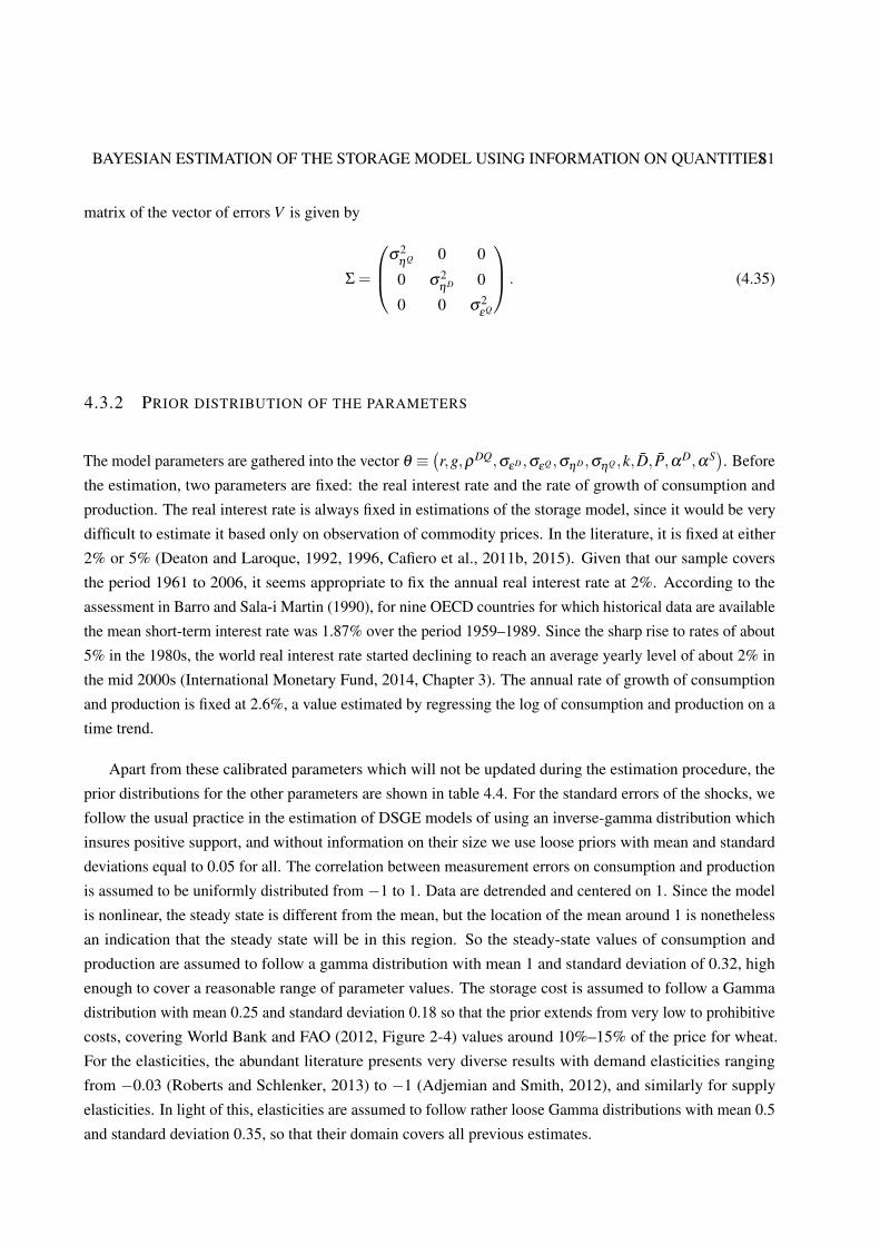
BAYESIAN ESTIMATION OF THE STORAGE MODEL USING INFORMATION ON QUANTITIES81
matrix of the vector of errors V is given by
Σ =
σ2ηQ 0 0
0 σ2ηD 0
0 0 σ2εQ
. (4.35)
4.3.2 PRIOR DISTRIBUTION OF THE PARAMETERS
The model parameters are gathered into the vector θ ≡(r,g,ρDQ,σεD ,σεQ ,σηD ,σηQ ,k, D̄, P̄,αD,αS
). Before
the estimation, two parameters are fixed: the real interest rate and the rate of growth of consumption and
production. The real interest rate is always fixed in estimations of the storage model, since it would be very
difficult to estimate it based only on observation of commodity prices. In the literature, it is fixed at either
2% or 5% (Deaton and Laroque, 1992, 1996, Cafiero et al., 2011b, 2015). Given that our sample covers
the period 1961 to 2006, it seems appropriate to fix the annual real interest rate at 2%. According to the
assessment in Barro and Sala-i Martin (1990), for nine OECD countries for which historical data are available
the mean short-term interest rate was 1.87% over the period 1959–1989. Since the sharp rise to rates of about
5% in the 1980s, the world real interest rate started declining to reach an average yearly level of about 2% in
the mid 2000s (International Monetary Fund, 2014, Chapter 3). The annual rate of growth of consumption
and production is fixed at 2.6%, a value estimated by regressing the log of consumption and production on a
time trend.
Apart from these calibrated parameters which will not be updated during the estimation procedure, the
prior distributions for the other parameters are shown in table 4.4. For the standard errors of the shocks, we
follow the usual practice in the estimation of DSGE models of using an inverse-gamma distribution which
insures positive support, and without information on their size we use loose priors with mean and standard
deviations equal to 0.05 for all. The correlation between measurement errors on consumption and production
is assumed to be uniformly distributed from −1 to 1. Data are detrended and centered on 1. Since the model
is nonlinear, the steady state is different from the mean, but the location of the mean around 1 is nonetheless
an indication that the steady state will be in this region. So the steady-state values of consumption and
production are assumed to follow a gamma distribution with mean 1 and standard deviation of 0.32, high
enough to cover a reasonable range of parameter values. The storage cost is assumed to follow a Gamma
distribution with mean 0.25 and standard deviation 0.18 so that the prior extends from very low to prohibitive
costs, covering World Bank and FAO (2012, Figure 2-4) values around 10%–15% of the price for wheat.
For the elasticities, the abundant literature presents very diverse results with demand elasticities ranging
from −0.03 (Roberts and Schlenker, 2013) to −1 (Adjemian and Smith, 2012), and similarly for supply
elasticities. In light of this, elasticities are assumed to follow rather loose Gamma distributions with mean 0.5
and standard deviation 0.35, so that their domain covers all previous estimates.
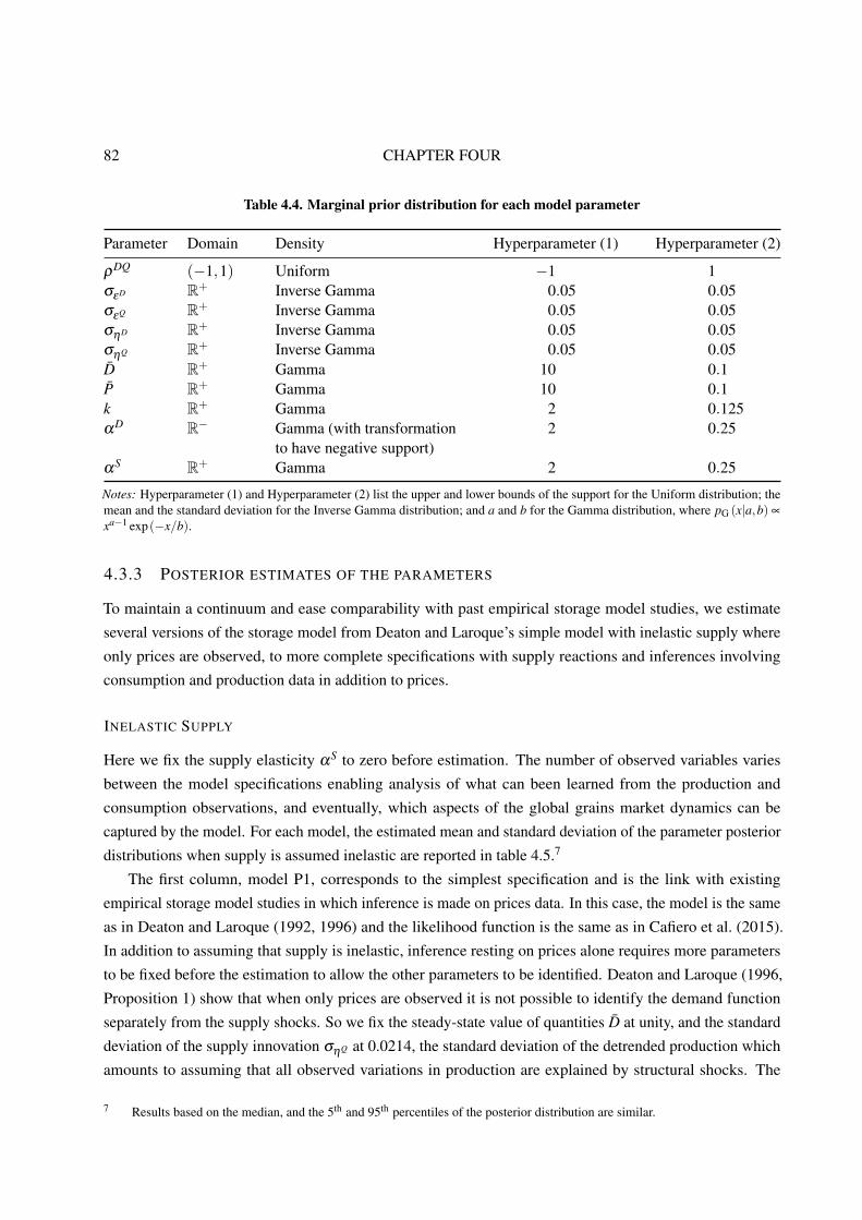
82 CHAPTER FOUR
Table 4.4. Marginal prior distribution for each model parameter
Parameter Domain Density Hyperparameter (1) Hyperparameter (2)
ρDQ (−1,1) Uniform −1 1σεD R+ Inverse Gamma 0.05 0.05σεQ R+ Inverse Gamma 0.05 0.05σηD R+ Inverse Gamma 0.05 0.05σηQ R+ Inverse Gamma 0.05 0.05D̄ R+ Gamma 10 0.1P̄ R+ Gamma 10 0.1k R+ Gamma 2 0.125αD R− Gamma (with transformation
to have negative support)2 0.25
αS R+ Gamma 2 0.25
Notes: Hyperparameter (1) and Hyperparameter (2) list the upper and lower bounds of the support for the Uniform distribution; themean and the standard deviation for the Inverse Gamma distribution; and a and b for the Gamma distribution, where pG (x|a,b) ∝
xa−1 exp(−x/b).
4.3.3 POSTERIOR ESTIMATES OF THE PARAMETERS
To maintain a continuum and ease comparability with past empirical storage model studies, we estimate
several versions of the storage model from Deaton and Laroque’s simple model with inelastic supply where
only prices are observed, to more complete specifications with supply reactions and inferences involving
consumption and production data in addition to prices.
INELASTIC SUPPLY
Here we fix the supply elasticity αS to zero before estimation. The number of observed variables varies
between the model specifications enabling analysis of what can been learned from the production and
consumption observations, and eventually, which aspects of the global grains market dynamics can be
captured by the model. For each model, the estimated mean and standard deviation of the parameter posterior
distributions when supply is assumed inelastic are reported in table 4.5.7
The first column, model P1, corresponds to the simplest specification and is the link with existing
empirical storage model studies in which inference is made on prices data. In this case, the model is the same
as in Deaton and Laroque (1992, 1996) and the likelihood function is the same as in Cafiero et al. (2015).
In addition to assuming that supply is inelastic, inference resting on prices alone requires more parameters
to be fixed before the estimation to allow the other parameters to be identified. Deaton and Laroque (1996,
Proposition 1) show that when only prices are observed it is not possible to identify the demand function
separately from the supply shocks. So we fix the steady-state value of quantities D̄ at unity, and the standard
deviation of the supply innovation σηQ at 0.0214, the standard deviation of the detrended production which
amounts to assuming that all observed variations in production are explained by structural shocks. The
7 Results based on the median, and the 5th and 95th percentiles of the posterior distribution are similar.
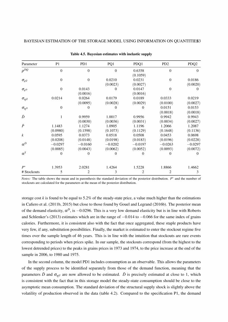
BAYESIAN ESTIMATION OF THE STORAGE MODEL USING INFORMATION ON QUANTITIES83
Table 4.5. Bayesian estimates with inelastic supply
Parameter P1 PD1 PQ1 PDQ1 PD2 PDQ2
ρDQ 0 0 0 0.6358 0 0(0.1059)
σεQ 0 0 0.0210 0.0231 0 0.0186(0.0023) (0.0027) (0.0020)
σεD 0 0.0143 0 0.0147 0 0(0.0016) (0.0016)
σηQ 0.0214 0.0264 0.0179 0.0189 0.0333 0.0219(0.0095) (0.0028) (0.0029) (0.0100) (0.0027)
σηD 0 0 0 0 0.0151 0.0153(0.0018) (0.0018)
D̄ 1 0.9959 1.0017 0.9956 0.9942 0.9943(0.0030) (0.0036) (0.0031) (0.0034) (0.0027)
P̄ 1.1483 1.1274 1.0905 1.1196 1.2066 1.2087(0.0980) (0.1598) (0.1073) (0.1129) (0.1648) (0.1136)
k 0.0595 0.0373 0.0518 0.0508 0.0453 0.0698(0.0208) (0.0148) (0.0198) (0.0183) (0.0196) (0.0228)
αD −0.0297 −0.0160 −0.0202 −0.0197 −0.0263 −0.0297(0.0085) (0.0043) (0.0062) (0.0052) (0.0093) (0.0072)
αS 0 0 0 0 0 0
P∗ 1.3953 2.0281 1.4264 1.5228 1.8866 1.4662# Stockouts 5 2 3 2 2 3
Notes: The table shows the mean and in parenthesis the standard deviation of the posterior distribution. P∗ and the number ofstockouts are calculated for the parameters at the mean of the posterior distribution.
storage cost k is found to be equal to 5.2% of the steady-state price, a value much higher than the estimations
in Cafiero et al. (2011b, 2015) but close to those found by Gouel and Legrand (2016b). The posterior mean
of the demand elasticity, αD, is −0.0296. This is a very low demand elasticity but is in line with Roberts
and Schlenker’s (2013) estimates which are in the range of −0.014 to −0.066 for the same index of grains
calories. Furthermore, it is consistent also with the fact that once aggregated, these staple products have
very few, if any, substitution possibilities. Finally, the market is estimated to enter the stockout regime five
times over the sample length of 46 years. This is in line with the intuition that stockouts are rare events
corresponding to periods when prices spike. In our sample, the stockouts correspond (from the highest to the
lowest detrended prices) to the peaks in grains prices in 1973 and 1974, to the price increase at the end of the
sample in 2006, to 1980 and 1975.
In the second column, the model PD1 includes consumption as an observable. This allows the parameters
of the supply process to be identified separately from those of the demand function, meaning that the
parameters D̄ and σηQ are now allowed to be estimated. D̄ is precisely estimated at close to 1, which
is consistent with the fact that in this storage model the steady-state consumption should be close to the
asymptotic mean consumption. The standard deviation of the structural supply shock is slightly above the
volatility of production observed in the data (table 4.2). Compared to the specification P1, the demand
84 CHAPTER FOUR
function has a much steeper slope at −0.016. Combined with a lower storage cost estimated at 3.31% of
the steady-state price, the inferred cutoff price P∗ over which inventories are sold out is 45% higher, which
decreases the estimated number of stockouts now limited to 1973 and 1974. The standard deviation of the
measurement error shock on consumption is of the same size as the volatility of consumption observed in
the data, so the storage model explains little of the variation in consumption. This is expected given the low
correlation observed between consumption and price.
In the specification PQ1, we use production as the observable rather than consumption, and assume
only one structural shock. Compared to the specification PD1, it leads to a lower standard deviation of the
posterior for σηQ , consistent with the fact that production is more directly informative than consumption
about the production shock. Compare to PD1, demand is slightly more elastic to price, and storage is more
costly (4.7% of the estimated steady-state price) but the differences are mostly all within the ranges of the
standard deviations of the estimates, except for σηQ . Nonetheless, these differences lead to a lower cutoff
price P∗ implying the occurrence of a third stockout in 2006.
The specification PDQ1 includes all available observables. It leads to estimates that are close to the
specifications PD1 and PQ1. This specification confirms that half of observed production fluctuations
can be explained by structural shocks with the other half accounted for by measurement errors. As for
PD1, the measurement error on consumption is substantial and would account for almost all observed
consumption changes. There is a significant correlation coefficient of the measurement error on consumption
and production: ρDQ = 0.64. This is consistent with the way these data are collected, with reasonably
thorough surveys of production, and estimates for consumption that partly depend on production estimates.
We turn next to specifications PD2 and PDQ2 which feature two structural shocks: one on consumption
and one on production. In these cases, a closed-form likelihood function with measurement errors on
consumption is not possible. We assume that consumption is perfectly observed, and is the sum of a
deterministic demand function and a structural shock. If we compare the specifications PD2 and PD1, what
is captured in PD1 in the measurement error on consumption is accounted for now by the structural shock.
Surprisingly, this leads also to a much larger structural production shock with a posterior mean for σηQ of
0.0333, an estimate which far exceeds the observed volatility in production. The estimation of σηQ is lower
under the specification PDQ2 which uses production as an observable. Overall, the specifications allowing
for two structural shocks lead to estimated net supply shocks (ηQ−ηD) larger in size than their counterparts
with one shock (PD1 and PDQ1) which implies a more elastic demand function, closer to Roberts and
Schlenker’s estimates.
ELASTIC SUPPLY
So far the literature on estimation of storage models has focused on models with inelastic supply because
prices were the only observables; this does not permit estimation of demand and supply elasticities. By using
consumption and production as additional observables we can estimate models with elastic supply.8
8 The sole observation of consumption is not informative enough to deliver sound estimates when the model has elastic supply.Hence, the PD1 and PD2 specifications are no longer considered in the subsequent estimations.

BAYESIAN ESTIMATION OF THE STORAGE MODEL USING INFORMATION ON QUANTITIES85
Theoretically, speculative storage and elastic production show interesting interactions.9 In the absence
of storage, the model collapses to Muth’s (1961) model where planned production is constant and equal to
its steady-state value because the expected price is constant. As soon as speculative storage operates, the
expected price and planned production varies. A high stock level weights on the expected prices, and by
extension, on the expected profits from production, along with the level of effort invested in new production.
Conversely, low stock levels lead to high expected prices and high levels of planned production, with an
upper limit attained when stocks are null. Because production adjusts to the expected price and helps alleviate
future scarcities, stock levels are less responsive to current availability. For various calibrations, Wright and
Williams (1982) show that a model with elastic supply leads to lower price volatility than the same model
with inelastic supply. This means that with elastic supply, lower stock levels will be required to fit the same
price volatility in the data. This translates to the estimation (see table 4.6) of higher storage costs and lower
cutoff prices than for the corresponding inelastic specifications. For the PDQ1 and PDQ2 specifications this
leads to five stockouts, in 1973–5, 1980, and 2006, while in the PQ1 specification there is a sixth stockout in
1979.
Table 4.6. Bayesian estimates with elastic supply
Parameter PQ1 PDQ1 PDQ2
ρDQ 0 0.6192 0(0.1115)
σεQ 0.0209 0.0231 0.0189(0.0023) (0.0028) (0.0020)
σεD 0 0.0145 0(0.0016)
σηQ 0.0189 0.0194 0.0224(0.0029) (0.0029) (0.0029)
σηD 0 0 0.0150(0.0017)
D̄ 0.9978 0.9921 0.9903(0.0038) (0.0032) (0.0029)
P̄ 1.3616 1.4016 1.4301(0.1356) (0.1381) (0.1404)
k 0.2045 0.1918 0.1943(0.0887) (0.0824) (0.0823)
αD −0.0218 −0.0198 −0.0300(0.0065) (0.0055) (0.0077)
αS 0.0560 0.0507 0.0492(0.0290) (0.0270) (0.0285)
P∗ 1.2811 1.3804 1.3713# Stockouts 6 5 5
Notes: The table shows the mean and in parenthesis the standard deviation of the posterior distribution. P∗ and the number ofstockouts are calculated for the parameters at the mean of the posterior distribution.
9 See Wright and Williams (1982) for a thorough description of the effects of modeling supply responsiveness in the dynamicsimplied by the model.
86 CHAPTER FOUR
For the same specifications, the estimations with elastic supply are similar to the estimations with inelastic
supply for almost all parameters except the steady-state price and the storage cost; both of which increase
significantly. Expressed as a percentage of the steady-state price, storage costs are of the order of 14%, a
value consistent with the World Bank and FAO (2012). Supply elasticities are estimated to be around 0.05,
so supply is twice as elastic as demand. These supply elasticities are in the lower range of the values in the
literature. Compared to Roberts and Schlenker (2013), they are twice as low. Roberts and Schlenker (2013)
estimate the supply elasticity as being between 0.085 and 0.116.
While most parameters are precisely estimated, the storage cost and supply elasticity are estimated with
limited precision. The standard deviations of the posterior distribution of storage cost and supply elasticities
are close to 43% and 53% of their respective means. Storage cost is the least precisely estimated parameter
in the inelastic case, which can be explained by the fact that beyond very small values the likelihood function
is quite flat with respect to storage cost. However, the standard deviation of k is much higher in the elastic
case. This likely stems from the fact that storage and elastic production are substitutes for explaining price
volatility. The observation of production should help choose between the two processes but given the size
of the measurement error on production, its informativeness is probably limited which explains the lack of
precision of the estimates.
Figure 4.3 summarizes the estimation results visually by plotting the prior distribution, and the posterior
distributions of the inelastic and elastic PDQ2 models. It confirms that the posterior distributions are the
same in the inelastic and elastic cases, except for P̄ and k. All parameters are estimated to be significantly
different from zero. Except for the storage cost in the elastic case, the posterior distributions are different
from the prior distributions. The similarity of the prior and posterior for storage cost if the model features
elastic supply confirms a potential problem of identification.
4.4 CONCLUSION
This chapter proposed a new estimation strategy for the rational expectations storage model. In addition
to prices, it adds to the observable variables consumption and production. This allows the identification of
parameters not recoverable if the inference rests on prices alone, and enables estimation of a richer storage
model with elastic supply and two structural shocks. The estimation method takes its inspiration from recent
developments in the estimation of DSGE models. It uses Bayesian econometric methods which are more
suited to these types of dynamic models than frequentist methods, which are more likely to experience
difficulty to find a global maximum. To ease comparability with the results in the literature, we started the
estimations with a specification close to Cafiero et al. (2015), with inelastic supply and prices as the only
observables. We introduced more observables gradually, and relaxed the assumption of inelastic supply. The
variety of model specifications estimated allowed us to identify the contribution of each set of observables to
the results. In order to have a benchmark against which to compare our results, the model was estimated on
the same set of data as in Roberts and Schlenker (2013): the market for the caloric aggregate of maize, rice,
soybeans, and wheat from 1961 to 2006.
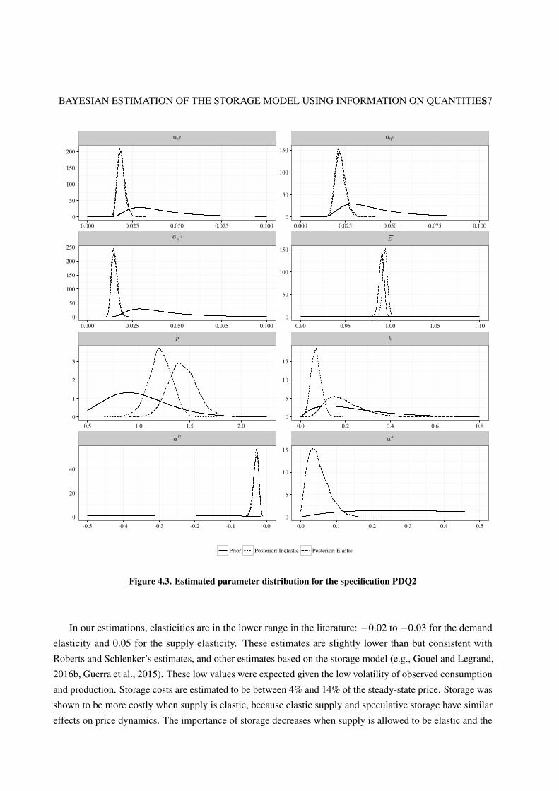
BAYESIAN ESTIMATION OF THE STORAGE MODEL USING INFORMATION ON QUANTITIES87
σεQ σηQ
σηD D
P k
αD αS
0
50
100
150
200
0
50
100
150
0
50
100
150
200
250
0
50
100
150
0
1
2
3
0
5
10
15
0
20
40
0
5
10
15
0.000 0.025 0.050 0.075 0.100 0.000 0.025 0.050 0.075 0.100
0.000 0.025 0.050 0.075 0.100 0.90 0.95 1.00 1.05 1.10
0.5 1.0 1.5 2.0 0.0 0.2 0.4 0.6 0.8
-0.5 -0.4 -0.3 -0.2 -0.1 0.0 0.0 0.1 0.2 0.3 0.4 0.5
Prior Posterior: Inelastic Posterior: Elastic
Figure 4.3. Estimated parameter distribution for the specification PDQ2
In our estimations, elasticities are in the lower range in the literature: −0.02 to −0.03 for the demand
elasticity and 0.05 for the supply elasticity. These estimates are slightly lower than but consistent with
Roberts and Schlenker’s estimates, and other estimates based on the storage model (e.g., Gouel and Legrand,
2016b, Guerra et al., 2015). These low values were expected given the low volatility of observed consumption
and production. Storage costs are estimated to be between 4% and 14% of the steady-state price. Storage was
shown to be more costly when supply is elastic, because elastic supply and speculative storage have similar
effects on price dynamics. The importance of storage decreases when supply is allowed to be elastic and the
88 CHAPTER FOUR
number of stockouts increases. These preliminary results tend to confirm that our Bayesian approach is a
reliable econometric method for structural estimations of the storage model.
In this preliminary version of the work we made assumptions to permit the likelihood function of the
storage model to take an analytic form. This involves severe restrictions: unlike quantities prices were
assumed to be observed without noise, and it was not always possible to estimate measurement errors and
structural shocks jointly. These restrictions will be lifted in the final version of the study which will present
estimations with more general specifications.
The new estimation methods for the storage model proposed in this chapter constitute an important
innovation; however one of their main benefits may be the new perspectives they open for this model.
Deaton and Laroque (1992, 1996) rejected the storage model for its inability to fit the serial correlation
in prices. This problem has been solved in recent works but with an estimation method which allows us
to use all observables to fit the model, it is likely that the storage model’s ability to fit the behavior of the
observables will decrease with the number of observables. The dimensions where the model fails will open
the way to new theoretical developments to improve the model fit. We have seen similar developments in the
econometrics of DSGE models where extra elements have been added to the basic RBC model to improve its
fit (Fernández-Villaverde, 2010). In the case of our estimations, the standard deviations of the measurement
errors on consumption and production are large and could explain most the observed variations. So the
current specification of the storage model is not able to account well for the dynamics of quantities, and
should be extended with this shortcoming in mind.
CHAPTER 5
THE CROWDING-OUT EFFECT OF STORAGE ON INVESTMENT:
EVIDENCE FROM THE CRUDE OIL SECTOR
Chapter written with Assia Elgouacem except for the preamble.
PREAMBLE:
ROLLER COASTER IN THE OIL INDUSTRY
5.1 PREAMBLE
UNPREDICTABLE BY NATURE
It is fair to say that guessing what would be the oil price no further than a couple of months ahead is a perilous
if not impossible exercise. At best, one can come up with a rather loose 95% confidence interval. Hamilton
(2009) would not disagree with me on this when he shows that neither the U.S. nominal interest rates nor the
U.S. GDP growth rates are significantly helpful when it comes to forecast the quarterly real oil price change
over the 1970-2008 period. Trying to predict the level instead of the change in prices is of no use since both
the Dickey-Fuller and KPSS tests fail to reject the unit root hypothesis at the 5% level of significance. In the
end he concludes that crude oil prices follow a random walk with drift. From a statistical standpoint it just
means that for a given standard deviation σ of the price change over the whole sample length, the logarithm
of the real oil price p = log(P) in n quarters into the future is expected to fall within the 95% lower and upper
bounds defined as [p±1.96σ√
n]. Given a price at $115 a barrel as of the first quarter of 2008–e.g., the last
data point of the sample he used–that leaves somebody trying to guess the price value in the next quarter with
a range as large as $85 to $115 per barrel. The author could not have put it better when extending the forecast
until 2012:Q1 he ends up saying that the price per barrel can well be as low as $34 or as high as $391.
In the first quarter of 2012, the real oil price was in the $85-90 region. At that time, very few people
would have bet that four years later (e.g., in 2016:Q1) the WTI crude oil price would lie below the $30
a barrel barrier. However, such an erratic behavior in the price of crude oil does not mean variations are
completely irrational. Instead, a thorough understanding of price dynamics of commodities such as oil relies
on a close look to the market fundamentals of supply, demand and storage which eventually are governing the
global price formation. With this in mind, I will turn now to try to explain why, after having posted records
upon records during more than a decade, crude prices collapsing to the bottom values ranging from $25 to
I would like to note that this short introductory section is largely inspired by blogs readings and more particularly both http://www.oilslick.com/ and http://oilprice.com which I strongly recommend.
THE CROWDING-OUT EFFECT OF STORAGE ON INVESTMENT 91
$30 a barrel reached at the beginning of 2016 is not too big a surprise. Similarly, a crude price well above
$100 a barrel as of 2020 seems quite plausible.
A RESILIENT SUPPLY
As in many industries involving substantial upstream investment costs, a large proportion of them could even
be described as sunk costs, the oil production has trouble to adjust so as to track closely the corresponding
demand. Indeed, in the short run it is almost impossible to satisfy a sudden increase in the oil consumption
apart from any excess production capacity and inventories of limited availability. Inversely, the same is true
also when it comes to balance a drop in demand. Such a low supply reaction has to do with (i) the long lead
times it takes for oil from a new field discovery to be extracted and actually come online,1 (ii) the hysteresis
effects stemming from both the significant capital and exploration expenditures at stake, (iii) the strategic
behavior of suppliers willing to stay competitive in this hostile environment. There is an element of truth to
all of them so let us illustrate with concrete examples those explanations which have been studied at length in
the theoretical as well as the empirical economic literature as will be seen further in the chapter.
IRREDUCIBLE DELAYS
Supply dynamics in the oil sector are deeply constrained by capital and exploration (capex) costs considera-
tions. First, oil companies have to spend billion of dollars in the search for new oil deposits both located in
on-and offshore areas. Once discovered comes the exploitation phase which then again requires a significant
amount of time and investment. Indeed, before starting to drill, operators have to deal with administrative
procedures to get the operating license along with the credit lines from financial institutions given the size of
the sums involved. To get a general picture, since the early seventies no less than $172 billions of dollars a
year on average have been invested in capex activities in the oil sector alone as reported by the Rystad Energy
company. All of these risky ventures whose outcomes are very uncertain have to be supported by high spot
price levels and expected lasting for a while.
In addition, not only the upstream investments are significant but most of them are almost irreversible
since, once drilled, a well cannot be resold or at least at an extremely discounted price. It turns that it is
optimal for operators to wait for stable and optimistic future economic conditions before committing into the
development of new oil fields.2
In sum, the combination of hardly compressible lengths related to the diverse exploration and drilling
processes with the long periods of inaction caused by the real options mechanism primarily explain why fresh
oil discoveries cannot be expected to be delivered before at least 3 to 5 years according to the most optimistic
figures given by the oil industry experts. As a result, the supply falls short of demand leading prices to settle
at a higher level as long as a new stream of production flows and balances the market back. Nevertheless,
1 It is fair to say that these delays are widely reduced in the shale industry.2 The theoretical foundations have been laid out in the real options literature (Pindyck, 1991, Dixit, 1992) and an empirical
illustration is provided in Kellogg (2014).

92 CHAPTER FIVE
there exist also factors preventing output from decreasing in response to a lower demand adding to the overall
lack of supply flexibility, a point to which we will turn now.
STICKY PRODUCTION
Once the newly installed capital becomes productive and start flowing into the market, although technically
feasible a downward adjustment of production in response to an oil consumption slowdown is far from
being immediate too. Nonetheless, the reasons for such a stickiness in the decline of oil supply are of a
very different nature. First, oil producers, often heavily indebted, are desperate for cash flow needed to
meet their financial obligations and avoid bankruptcy. Then, they want to lose neither the benefit of their
licenses and leases, nor the products from wells which once completed and fractured cannot be capped and
tapped later. They also keep pumping to offset the inevitable depletion from old wells. These decisions are
supported further by the fact that operating costs are really tiny compared to those already devoted initially
in the capex development phases. Finally and rarely mentioned, chances are high that a large share of the
upcoming production has been hedged against a fall in prices sometimes for several years ahead using the
variety of financial instruments available from the forwards markets. This is why even if the spot price is
falling below the breakeven production costs of some oil reserves, the latter can remain profitable to the
operators concerned.3
Hence, between 2014 and the beginning of 2016 and despite high production costs and the sharp drop
of the crude market price, oil production from North America kept rising to the great displeasure of Saudi
Arabia whose supremacy has been challenged by the shale boom and which has seriously underestimated the
resilience of the North American oil industry. This leads us to explore the final force leaning against a quick
supply response to price variations, namely the market competition.
STRATEGIC BEHAVIORS
Competition in the oil industry is particularly fierce and have even been exacerbated over the past ten years
by the U.S.“shale” revolution. To some extent and at some points in the seventies and early eighties the
Organization Petroleum Exporting Countries (OPEC) might have been effective at controlling the supply and
thereby the price level worldwide.4 Since that time, however, evidences have tended to show that it is no
longer the case. The broad part of the explanation are of two types.
The first is internal to the cartel and rests on the existing difference between individual and collective
marginal profit. In short, to decide on a price target and exercise its market power the OPEC has to fix the
total production level implying a zero marginal profit for the group before agreeing to share the corresponding
quota between each of the members. The point is that each member has an incentive “to cheat”–e.g., to
produce more than its assigned level–breaking the initial agreement thus becoming irrelevant as illustrated in
3 As the very last futures contracts will expire this year, the “hedging effect” comes to an end bringing producers back to themarket reality while the U.S. production begins to reverse.
4 It has to be noted that OPEC succeeded to the “seven sisters” which is the name given to the seven big oil companies whichcolluded on prices and dominated the market during the first half of the twentieth century.
THE CROWDING-OUT EFFECT OF STORAGE ON INVESTMENT 93
Hamilton (2009), and elsewhere in the literature pointing to the overall lack of empirical evidences supporting
a significant “cartel effect” on the crude price (Alhajji and Huettner, 2000, Smith, 2005). Things are not
expected to change anytime soon as now we are closer to an explosion of the OPEC than a strengthened
cooperation, and despite the last estimation of the International Energy Agency (IEA) indicating that OPEC’s
share of the oil market has reached 34 percent, a level not seen since 1975. Indeed, the historical religious
tensions between Saudi Arabia and Iran is complemented by an economic rivalry since the latter is determined
to take advantage of the recent lifting of international sanctions by ramping up production to make up for the
lost market shares.5
Apart from the apparent failure of the OPEC members to agree on a production quota, the former role
of “swing producer” Saudi Arabia used to play is threatened by the emergence of new big entrants, namely
Russia, Canada and the U.S., which are not part of the OPEC nor willing to agree on prices. It results in a
radical change in the landscape of world oil supply with heightened competition between smaller producers
fighting for market shares, reluctant to cut production whenever demand is softening and with no alternative
but to commit into a race to efficiency gains to stay competitive. For instance in the U.S. shale oil industry
the depletion rate of wells along with the marginal production costs have been almost halved since 2012
contributing to the outstanding resilience of shale oil producers.
Overall, the combination of lumpy and irreversible spending in the capex development stages with a rigid
supply and financially constrained operators struggling to hold on their market share and stay in business,
can turn even the slightest slowdown in the growth of oil consumption into a real glut exactly like the one
experienced since 2014.
AN OPAQUE DEMAND
If the dynamics of production in the oil sector is fairly well featured it is far from being the case concerning
the demand side of the picture. All one can say is that it is almost as inelastic as the supply in the short-run
and that the economic literature used to draw a distinction between speculative demand and demand for
immediate consumption.
VARIABLE ELASTICITIES
Whether directly or indirectly used, oil is an input for all sectors of the economy so that to assess and predict
the oil consumption the IEA has no choice but relying on some key macroeconomic variables governing
the final demand and the corresponding elasticities.6 Demography and economic activity are among the
prominent drivers. Indeed, if the data show anything, it is that the consumption of oil in a given country
closely tracks the prevailing growth in income per capita. As the living standard are improving, people can
afford motorized transportation, buy more consumer electronics and other household appliances while both
public and private infrastructures keep pace with the economic growth. All of these elements fuel the final
5 Additional tensions do exist between Saudi Arabia and other member states such as Venezuela which really suffer from thecurrent levels of crude price.
6 Here, the elasticity has to be interpreted as the variation of quantity demanded following a change in the variable in question.
94 CHAPTER FIVE
growth in petroleum consumption. Unsurprisingly, China alone accounts for the lion share in the dramatic
rise of oil consumption observed since the early nineties, passing from a low 3.8% to 12.8% of the oil demand
worldwide which soared approximately from 21 to 28 billion of barrels between 1990 and 2013.7 And now
that China’s economy is facing serious headwinds, all eyes are turning to India which is expected to take over
with its 1.2 billion of inhabitants and its steady double digit rate of growth in Gross Domestic Product (GDP).
It is also worth mentioning that, as the yearly per-capita oil consumption in China or India is five times lower
than in Germany and even ten times than in the U.S., chances are high that the last IEA’s yearly global growth
rate figure of 1.6 billion/day can climb to much higher levels in the coming years. Still, China and possibly
even more India will be the main growth engines in global oil demand for at least the next decade.
However, the more challenging in the demand assessment process is to estimate the elasticities. Indeed,
they are many forces behind the quantity consumed and it is hard to disentangle their respective contribution
and even more so since elasticities are varying both over time and across countries depending on the level
of economic developments.8 Actually the reported estimates are often a mix between the true elasticity of
demand for immediate consumption with the speculative one for storage, the second central pillar of oil
demand which must not be overlooked.
SPECULATIVE DEMAND
If the storage mechanism and its effects in the price dynamics are straightforward to understand and well
documented, the fact remains that measuring with accuracy the levels of stocks is almost impossible. Indeed,
abstracting from the underground inventories commonly categorized as “proven reserves”, the global stocks
held above ground should include (i) the industrial quantity stockpiled by refiners, (ii) those hold by states and
(iii) the too often neglected “floating storage” (e.g., on tankers). Let us examine each in turn the motivations
driving the accumulation of inventories.
In the same way as for producers hedging against a fall in prices, refiners and more broadly industrial
consumers tend to protect their future supplies and avoid costly disruptions in the transformation process
of crude oil. That, in turn, lead them to buy and store output in advance whenever the expected rise in the
price is sufficient to cover the physical and interest costs incurred. Although it is the most visible and known
component of storage demand, that its key determinants are well established and theoretically grounded,
wild variations of large magnitudes still happen. The latest case can be found in China where following a
legislation change dating back from July 2015, the private refineries known as “teapots” have been allowed
to operate directly and independently in the international market, which translated into Chinese record high
numbers of crude imports reaching about 125 million tons in the first four months of 2016, up 12% from
the same period a year ago and of which teapots alone account for 15%.9 Such additional demand had a
considerable impact in preventing the spot crude price from tumbling even further, even participating into its
last spring rebound.
7 The figures are available from the IEA’s databases https://www.iea.org/statistics/statisticssearch/.8 A summary of demand and income elasticity values in both the short and long-run is provided in Hamilton (2009).9 The figures are taken from the Wall Street Journal.
THE CROWDING-OUT EFFECT OF STORAGE ON INVESTMENT 95
Onshore tanks are not the only place where commodities can be piled up especially when, as is occurring
now, continental storage capacities are stretched to the limits. The amounts involved with the storage at
sea, albeit smaller by an order of magnitude, can play a major role in the price behavior and should not be
relegated as a simple back-up solution. Indeed, unlike refiners most of the market practitioners are traders
who actually do not take on deliveries, acting instead as pure speculators by closing or rolling over time
their positions before the contract expiration. To benefit at full from the positive gap between futures and
spot price–known as a contango situation–traders do not hesitate to play with the sailing speed waiting for a
tightening in the market conditions leading to a price bounce, a strategy which has long been part of their
toolkit. If the volume of purchases is large enough it might widen artificially the contango by pushing up the
futures prices before the true supply and demand fundamentals finally take over.10
Lastly, much more important in size but far less transparent are the inventories run by the states themselves.
It is no exaggeration to say that having access to a secure supply of oil is absolutely vital for a modern
economy since oil shortages can trigger riots or even revolution and wars as has been the case more than once
in history. Though oil issues have always been high on the political agenda it seems that we have entered a
new era. Indeed, fears from the looming peak oil associated with an ever-increasing world price sparked a
race to the energy self-sufficiency. If the U.S. government primarily bet on its own huge non-conventional oil
reserves, China actually follows an alternative strategy of buying petroleum output in advance to capitalize
on the current crude weakness. Therefore, in addition of buying as much oil assets as they can all through
the world (e.g., platform, fields, companies,...), of signing a deal with Hugo Chavez granting them a priority
access to the Venezuelan oil in exchange for massive investments into the country’s infrastructure, China
is building tremendous stocks. By 2020, the official target alone is to hold 90 days of supply (e.g., about
1.5 billion of barrels) within the Strategic Petroleum Reserves (SPR). One never knows with China but the
fact that its crude imports grew at a record pace over the first half of 2016 indicates that the country is likely
hoarding crude (nearly 95 million of barrels in the first quarter according to Bloomberg). Adding to this the
fact that India which imports 75% of the petroleum it consumes is following the same strategy and one ends
up with substantial physical quantities removed form the market and carried over to meet further needs, thus
impacting both the short and long-run price dynamics. Put it another way, the public storage demand even
though out of sight must not be out of mind.
A BRIGHT OR BLEAK OUTLOOK?
In essence, the oil market is characterized by a sluggish supply and a multifaceted demand really hard to
square. In addition, both of them are very inelastic, in the short-term at least. Bringing into the overall picture
the occurrence of shocks affecting both the supply and the demand sides of the global oil market and the
resulting final cocktail can do nothing but induce steep and large price swings in the short to medium-run.
Finding your way in these successions of booms and bust episodes is a tricky task, to put it mildly. As I
10 Critics of the “financialization” of commodity markets often blamed speculators for their destabilizing effect on prices. Thescientific community is deeply torn apart by this issue between the empirical studies showing the significant role speculation isplaying in the volatility of commodity prices (Singleton, 2014, Basak and Pavlova, 2016) and, inversely, those arguing that ithas no or very little impact (Kilian and Murphy, 2014, Knittel and Pindyck, 2016).
96 CHAPTER FIVE
have tried to show so far the better and wiser perhaps is to stick to the market fundamentals which ultimately
dictate the prices in the longer term. So, let us do it now in an attempt to answer the question of where the oil
price is heading to?
On the bearish camp, the arguments rest on (i) the record high-levels of inventories likely to cap any
crude price upticks for several months into the future, (ii) the fast rise in the Iranian production coupled with
more and more efficient U.S. shale oil producers ready to restart drilling as soon as the price is crossing the
$50/barrel barrier, as suggested by the modest increases in the U.S. rigs count in the last few weeks, (iii) the
stance in the U.S. monetary policy toward a normalization of interest rates and post-Brexit uncertainties which
both in strengthening the dollar value are weighing on the dollar denominated oil and (iv) the pessimistic
view regarding the global economic growth following the “great stagnation” theory of Tyler Cowen. It turns
that the market is still widely oversupplied and the last four-month price recovery is nothing but a fortunate
conjunction of circumstances mainly caused by the temporary supply outages which occurred in Canada
(wildfires), Nigeria (Avengers attacks), Venezuela (near bankruptcy) and Libya (political instabilities).
To support their view, the bullish advocates point to (i) the huge slashes in capex investment expected
to exceed 1 trillion and even more depending on the length of the current supply glut, (ii) the no fewer
than 350,000 workers which have been fired in the oil sector across the world since 2014, most of whom
will not come back as they have moved on to other industries, (iii) all the equipment idled and scrapped
during long periods of time which need extensive repairs before becoming productive anew, and (iv) the
lenders scalded by the heavy losses incurred so far and now more than ever reluctant to open new credit
lines. The combination of massive layoffs, severe cancellation or postponing of new development projects
and a drying-up of credit, will trim for a while the production capacities even if there is a spectacular price
rebound. In other words, by leaving the oil sector with loans, labor and equipment shortages, the last crude
crash have sowed the seeds for a sharp rally in prices as soon as 2020, given the strains on supply imposed by
the emerging economies, China and India ahead.
All in all, if the mainstream view among investors is a crude price fluctuating between $40 to $60/barrel
before climbing up again around $100 by 2020, the current market fundamentals do not look crystal clear to
everyone. Indeed, the most bearish forecasts stand to a crude price sliding to as low a level as $10 to $20 per
barrel by the fall of this year while, inversely, the most optimistic predictions expect the spot price reaching
the $80/barrel mark as early as 2017. These upper and lower bounds on prices define an amazingly similar
interval as the aforementioned 95% confidence interval when the price was assumed to follow a random
walk. Sharp booms and busts cycles are definitely inherent to commodity markets and oil is no exception.
Concerning the latter, the only thing that can be expected is a shortening of the price cycles due to the
recent U.S. shale revolution. That is why, rather than trying in vain to predict the unpredictable, theoretical
and empirical economic research must keep on building models, whether purely statistical or theoretical,
with or without microeconomics foundations, which are internally consistent and able to deliver insightful
explanation with respect to the behavior of prices on both the spot and forward markets.
THE CROWDING-OUT EFFECT OF STORAGE ON INVESTMENT 97
5.2 INTRODUCTION
The preamble could not better illustrate the fact that navigating the extremely volatile commodity markets
cannot but rely on relevant dynamic models resting on sound microeconomic foundations. Specifically,
these frameworks must featured the decisions of individual agents made over time in reaction to unexpected
shifts in the supply and demand fundamentals. In commodity markets, the crucial trade-offs faced by the
various actors have to do with investment and storage. It is no surprise then if, to assess the supply and
demand balance of crude oil, the practitioners look closely at the inventory levels and rig counts, a metric
often used to proxy the level of capital expenditure. Lastly, these are forward-looking decisions which often
involve substantial amounts of money and sunk costs. This mainly explains why, over the past few decades,
storable commodity markets have seen tremendous growth in the type, scope, and maturity of tradeable
forward contracts, which typically offer an appreciated price insurance to all the market participants in such
an uncertain economic environment. Hence, the interaction between the physical market and the future
market warrants a theoretical framework able to represent with accuracy a consistent relationship between
market fundamentals and their corresponding spot and futures prices.
Models of firm investment in the macroeconomic literature have been used to study the implications
of firm level nonconvexities for aggregate investment dynamics. Along the same lines, real option theory
has been applied to investment models with nonconvex adjustment costs as developed in Dixit and Pindyck
(1994) but the link between the physical market and the corresponding spot and futures prices has not been
studied explicitly. On the other hand, competitive storage models, and in general term structure models of
commodity markets, have addressed the link between market fundamentals and prices, yet mostly abstracting
from the firm’s investment decision. Additionally, empirical validation of the underlying theories has begun
at a time when most forward markets were still in their infancy and therefore widely overlooked. In light
of the ever-increasing prominence of financial markets, it is fair to say that valuable insights can be gained
also from the finance literature which focuses on the links between physical and financial markets, namely
the relationships between the market fundamentals and the return on different commodity futures contracts.
The idea being that futures markets provide a suitable data laboratory for real time testing of the dynamics
implied by such a forward-looking model.
This chapter aims at connecting and building upon three strands of the finance and economics literature
so as to feature the essential structural forces driving the commodity price in the world market. In particular
it hones in on the interaction between storage and investment by showing that the presence of storage
brings forth features in the investment and commodity price dynamics that cannot be accounted for when
focusing only on investment. Even more noticeable, exploiting the positive relationship between the levels of
inventories and the forward price volatility, we find that storage has a crowding-out effect on investment.11
The crude oil market will be used as a guideline illustration since it embodies, fairly well, this crowding-out
phenomenon as well as the occurrence of booms and busts cycles characterizing the prices behavior of most
commodities.
11 This positive correlation has even been empirically validated in Fama and French (1988) and Ng and Pirrong (1994).
98 CHAPTER FIVE
The results shed light on (i) the importance of introducing storage in an irreversible investment model
to generate the price and investment patterns observed in the data, (ii) the key role of the storage arbitrage
condition in dictating the impact of the irreversibility constraint on the timing of investment, while causing a
crowding-out effect of storage on investment, and (iii) the close relationship between the market fundamentals
and the term structure of forward curves given that the behavior of investment and storage are better reflected
in the slope of the forward curve rather than in the levels of spot and futures prices which are mainly governed
by global business cycles. Nonetheless, if our theoretical framework captures well the core forces governing
the observed dynamics in the crude oil market it is unable to generate sufficiently persistent volatility in the
futures prices, a common issue of this type of dynamic commodity market models.
The core logic of the present study is straightforward. First, we look at the supply and study to what extent
the investment and its associated constraints (e.g., irreversibility and adjustment costs) can generate dynamics
in prices similar to those observed on the global commodity markets. Then, turning to the demand side one
cannot ignore the large body of literature dedicated to the competitive commodity storage model showing the
key role of the speculative demand for inventories in the price discovery (Wright and Williams, 1982, Deaton
and Laroque, 1992, 1996). So far both literature on investment and competitive storage have been developed
quite independently of one another and we believe that bringing storage into the mechanics of the mere
capital accumulation model might help to come up with a consistent story about the functioning of global
commodity markets. The intuitive gist behind is that storage, by inducing conditional heteroskedasticity in
prices, is an endogenous source of time-varying uncertainty affecting the timing of investment decisions.
The impact of time-varying volatility on investment has been studied using real options pricing techniques,
elaborated in Dixit and Pindyck (1994).12 However, in this vein of the literature, heteroskedasticity in the
price is often imposed through an exogenous stochastic process.
We start by an extensive literature review, not only to get an overview of the existing structural dynamic
models aimed at understanding the behavior of commodity prices, but also to highlight the strong comple-
mentarities between them, which have yet to be taken into account. The effects of uncertainty, irreversibility
and capital adjustment costs have long been explored by the investment literature but rarely have they
exploited the capacity of inventory building to explain the dynamics of investment. For its part, the canonical
commodity storage model in the tradition of Gustafson (1958), often contends with either an inelastic supply
subject to random shocks (Deaton and Laroque, 1992, 1996, Cafiero et al., 2011b, 2015) or a rather crude
modeling of the supply response silent about the underlying capital accumulation mechanism (Wright and
Williams, 1982) and Gouel and Legrand (2016a); this is not surprising given that it has been primarily used
for analyzing the price behavior of agricultural products.
In both types of models, the agents have rational expectations, thereby taking forward-looking decisions
mirrored in the forward markets. This is precisely where the finance literature related to the hedging
strategies, in particular literature on normal backwardation and hedging pressure (both based on the market
fundamentals), comes to square the circle. In the descriptive analysis which follows we turn to the crude
12 See for instance Kellogg (2014) who exactly follows this approach in his empirical testing of the options value theory in the oilindustry.

THE CROWDING-OUT EFFECT OF STORAGE ON INVESTMENT 99
oil data and show to what extent investment and storage are complementary, but also and more broadly
we explore the interactions between the main variables involved at different time horizons. All of these
relationships portray a fairly consistent picture of the endogenous dynamics of the world oil market and thus
call for connecting investment and storage models while exploring the consequences on the term structure of
forward curves. Next, in an attempt to keep the essential features of each modeling strategy, we lay out the
general framework and derive the theoretical insights associated with the variety of economic restrictions,
namely the crucial non-negativity constraints on both the investment and storage. Lastly, relying on two
different capital accumulation models with irreversible investment depending on whether a speculative
storage demand is introduced, a series of simulations is provided to support the relevance of considering the
effects of storage on investment and to investigate in which dimensions the model does not work well.
The chapter falls as follows. Section 5.3 summarizes the three streams of literature along with the
underlying theories from which are derived most empirical models of commodity markets. Section 5.4
combines theories and data so as to paint a consistent picture of crude market dynamics. The general
framework with its associated theoretical insights are outlined in Section 5.5. Section 5.6 follows with
simulations and discusses the results. Section 5.7 concludes.
5.3 COMPLEMENTARY THEORIES: A LITERATURE REVIEW
In the economics and finance literature, the majority of dynamic equilibrium models explaining the commodity
price formation from market fundamentals rest on the investment and storage theories which provide the
microeconomic foundations behind the agents’ behavior. In addition, the forward-looking decisions made by
market participants are translated into the term structure of commodity futures prices, which in turn affects
the current actions. All these effects running both ways call for looking also under the hood of futures pricing
and forward market dynamics mostly studied in the finance literature. Highlighting synergies and drawing
insights from these theoretical developments is the purpose of this section.
5.3.1 INVESTMENT DYNAMICS AND CONSTRAINTS
Investment projects are more often than not met with large sunk costs, which make them partially if not mostly
irreversible. The cost of adjusting the capital stock has drawn much attention in the investment literature.
Evidence on the presence of nonconvex firm-level capital adjustment costs and investment irreversibilities
is extensive. Standard models of investment, such as q-theoretic models, generally assume that firms can
smoothly and continuously adjust their capital. Besides being more tractable, a model with convex adjustment
cost render investment less reactive to shocks and introduce serial correlation to its dynamics. This is indeed
an attractive feature in the model as it can deliver the persistence observed in the aggregate investment data.
However, when it comes to describing firm-level behavior, models with convex adjustment costs perform
poorly. Underlying the representative firm model of investment with quadratic costs is the assumption
that, while the individual firm might face non-convex adjustment costs resulting in lumpy firm-level invest-
ment patterns, irregularities are smoothed out through aggregation. Since firms adjust their capital stocks
100 CHAPTER FIVE
asynchronously, at the aggregate level lumpiness disappears and the capital stock adjustments can be well
described by convex adjustment costs. This reasoning provides the justification for the use of a representative
firm facing quadratic capital adjustment costs.
To assess the soundness of this short cut, models on aggregate investment turned to study microeconomic
investment decisions. Doms and Dunne (1998) cast doubt on the smoothness of capital adjustment at the firm
level using micro-data on firm investment distributions. Subsequently, Abel and Eberly (1994), Caballero and
Engel (1999) and Cooper and Haltiwanger (2006) as well as references therein, investigate the relevance of
different adjustment costs for both firm-level and aggregate investment dynamics. They show that firm-level
investment is indeed lumpy as they would like to adjust more when there is a capital shortage and less
when they have access to capital. These features of investment point to microeconomic nonlinearities, i.e.
both non-convex adjustment functions and investment irreversibility. Nevertheless, lumpiness of investment
at the firm-level has been found to disappear at the aggregate level. Thomas (2002) demonstrates how
general equilibrium price effects wash out firm-level investment lumpiness and thus pegs nonconvexities
in capital adjustment costs as inconsequential for business cycle analysis. More recently, Bachmann et al.
(2013) and Bachmann and Ma (2016) nuance the debate on the relevance of micro-economic lumpiness
for macroeconomics by pointing out that what can settle the issue is the relevant strengths of price and
adjustment cost responses. The difference between firm-level models of aggregate investment and those of
the “representative” firm is that the former are able to generate nonlinear aggregate investment. The presence
of a hazard rate of adjustment that depends on the gap between the firm’s level of capital and the desired
one is the key to matching higher moments of aggregate investment. Therefore as in Caballero (1999), these
microeconomic non-convexities generate an important “time-varying/history-dependent aggregate elasticity”
of investment to shocks by allowing changes in the synchronization of firms’ capital adjustments. Cooper
and Haltiwanger (2006) investigate the relevance of different adjustment cost specification for investment at
the firm, sector and aggregate levels. They found that investment whether at the firm or sector level is best
described by a model which includes non-convex capital adjustment costs as in Abel and Eberly (1994) and
Caballero and Engel (1999).
However, a more complete examination of the commodity markets dynamics requires looking at the
second pillar of the supply and demand fundamentals, namely the demand side in which storage is central.
5.3.2 THE COMPETITIVE STORAGE MODEL
A no less lengthy literature focuses on the effect of storage in the formation of commodity prices. The
competitive storage model with rational expectations and a non-negativity constraint on inventories in the
tradition of Gustafson (1958) has been the workhorse of neoclassical studies in the literature of commodity
price volatility. Deaton and Laroque (1992, 1996) pioneered its empirical validation by developing techniques
to confront the observed price data with a version of the model with inelastic supply modeled by either i.i.d.
or autocorrelated random shocks. Eventually they draw mixed conclusions. On one hand, it proves useful in
reproducing most of the prominent features observed in commodity prices (persistence, nonlinearity, positive
skewness and excess kurtosis) in particular as a result of the key non-negativity constraint on storage which
THE CROWDING-OUT EFFECT OF STORAGE ON INVESTMENT 101
brings forth two different price regimes. On the other hand, it is unable to match the very high levels of serial
correlations observed in commodity prices even after allowing for persistence in the supply disturbances.
Most of the critiques have been addressed through several recent improvements on both the numerical
(Cafiero et al., 2011b) and empirical fronts (Cafiero et al., 2015, Guerra et al., 2015).13
However, so far existing econometrics studies conducted on the storage model, in relying on information
taken from spot prices alone, have been limited to its starkest specification, that is without allowing for
neither structural demand shifts nor a supply reaction to prices although versions of the model with elastic
supply have existed for a long time.14 Indeed, Wright and Williams (1982) demonstrate the implications of
supply responsiveness in terms of the price behavior generated by the model. Interestingly, they show that
storage has a destabilizing effect on the expected price and in turn on the planned production, but also that it
is unclear whether planned production and storage act as substitutes or complements since the mean level of
storage is left virtually unchanged. Therefore, from an investment standpoint accounting for storage should
make it more volatile as its expected return is less certain. Put it another way, it is not so much the long-run
average of investment but its dynamics and timing which might be primarily impacted by the introduction of
storage into the framework.
Lastly, if most empirical studies of the storage model have been implemented on agricultural commodities
and using annual data due to the seasonality, the issues related to the interactions between investment and
storage might be more relevant for commodities such as petroleum or metals whose production often requires
costly and long investment lead times.15 Indeed, as stated by Gilbert (1995), these supply constraints should
translate into long periods of prices lying below the long-run average of production costs.
In this spirit and still in an effort of extending the fitting possibilities of the storage model, Dvir and
Rogoff (2014) build a version for the oil market embedding both elastic and inelastic supply regimes along
with persistent demand shocks. Specifically, their modeling accounts for a single trend in both demand and
production so that prices are left stationary. The model is then stationarized by scaling all quantity variables
by the aggregate income, measured by a global economic activity measure, assumed to be the major driver of
the growth in consumption. This set-up, with a rich structure of shocks, allow them to highlight the strong
conintegrating links between the prices and the market fundamentals of supply, demand and inventories as
predicted by the canonical storage model but also exhibited by the true data. Even more importantly perhaps,
they demonstrate that the correlation between prices and inventories can run in both directions depending on
whether or not supply is flexible enough to keep pace with the rising trend in demand. In the latter case, price
and inventories tend to move in the same direction.
Lastly, as briefly evoked in Chapter 2, given the forward-looking nature of both types of models, chances
are high that investment, storage and their subsequent interactions eventually are mirrored in the term
structure of commodity forward prices; a point the financial economists have long been recognized.
13 See chapter 2 for more on these recent developments.14 The lack of reliability and availability of data on quantities mostly explain why they have been overlooked until now. Taking to
the data on prices and quantities richer model specifications is precisely the topic of Chapter 3.15 From a strict statistical view point, another advantage is the possibility to work with monthly data given that, unlike the
agricultural products, this type of commodities are less subjected to the seasonality constraints.
102 CHAPTER FIVE
5.3.3 THE DETERMINANTS OF FUTURES PRICING
Although usually designed to model the risk premium of commodity futures contracts and assess the
performance of trading strategies, valuable insights can be gained from the literature on commodity futures
pricing which provide theoretical foundations to the behavior of prices on the futures market. Indeed, theories
of the determinants of speculators’ profit might help better understand the information which can be extracted
from futures prices and more broadly from the term structure of the futures market. Among them, only those
related to the fundamentals of supply, demand, and inventories, will be covered.
The first strand of the literature rests upon the theory of storage in the tradition of Kaldor (1939), Working
(1949) and Brennan (1958) which delivers a standard expression for the link between forward and spot prices
given by the following storage arbitrage equation:
Ft (T ) = St (1+Rt (T )))+Ct (T ) , (5.1)
where Ft (T ) stands for the forward price as of time t for delivery at time T , St is the spot price, Rt is the
interest cost of storage and Ct is the total net of interest cost of carry.16 Telser (1958) is among the first to
propose an empirical validation of this theory by documenting the close relationship between the inventory
levels and the basis (also called roll-yield) written as the spread between the spot and the nearest to maturity
future contract. More precisely, abundant stocks is regarded as a fair signal of a contango regime that is a
negative spread or an upward sloping forward curve. Also relying on the storage theory, Fama and French
(1988) complement the Samuelson hypothesis according to which (i) the volatility of forward prices has
to decline with the contract horizon and (ii) forward prices in contango are always less volatile than those
backwardated. Working with a set of metals and using the sign of the interest-adjusted basis as a proxy for
the levels of inventories (e.g., Ft − (1+ r)St), they demonstrate that whenever the levels of stocks is running
high (positive adjusted-interest basis), the spot and futures prices are as volatile. Part of the explanation has
to do with the lockstep variations of both current and expected spot prices linked by the storage arbitrage
equation (5.1).17 If inventories are running low, supply and/or demand shocks cannot be buffered by a release
of stocks which lead to variations of current spot prices to be greater than those of the futures prices for
which the market anticipates supply and demand responses. That is why Fama and French show that the spot
price of metals is more volatile around the business cycle peaks when demand is high and is satisfied by a
draw down of inventories.
Another stream of literature revolves around the Keynes-Hicks theory of normal backwardation stating
that, since hedgers are usually net short in the futures market (e.g., the number of selling positions exceeds the
buying one in the forward market), the future price deviations from the expected spot price can be attributed
to a risk premium rewarding the traders willing to hold the long positions. Nevertheless, the lack of empirical
16 Ct (T ) =W ft (T )+Rpt (T )−Cyt (T ). Ct (T ), total net of interest cost of carry, which can possibly include transportation andwarehousing fees W ft , risk premia Rpt and convenience yield Cyt . Following the literature of commodity storage model, wewill assume zero convenience yield and that agents are risk neutral and thus risk premia are zero.
17 In the basic storage model without convenience yield, whenever storage is positive, the adjusted-interest basis equals thephysical storage cost.
THE CROWDING-OUT EFFECT OF STORAGE ON INVESTMENT 103
evidence led to refinements allowing the hedgers to be either net-long or net-short in aggregate (Cootner,
1960).18 In the latter case, forward prices are below the spot price in a similar manner to the hypothesis
of normal backwardation. Inversely, when the number of hedging positions is net-long the forward curves
increase with time to maturity and the market is in contango providing the speculators an incentive to take
the opposite short positions. Hence, according to the hedging pressure hypothesis both backwardation and
contango are rational states of the futures market from the speculators standpoint. Using proprietary data
Dewally et al. (2013) give an illustration for crude oil, gasoline and heating oil. Specifically, they find a
systematic positive gain whenever a given trader is taking the opposite position in sign of the net hedger’s
one. Gorton et al. (2012) provides an optimization-based approach to endogenously model the basis along
with the risk premium. Integrating within the same two-periods framework both the theories of storage and
normal backwardation they empirically explore the connections between the inventory levels, the basis and
the risk premium. Running a series of regression on monthly futures and inventories data of 31 commodities,
they demonstrate that, as dictated by the storage theory, the relationship between the levels of stocks and
the futures basis is negative and convex. In addition they also show the predictive power along with the
negative correlation between the amount in store and the risk premium as posited by the theory of normal
backwardation, but do not find significant evidence in favor of the hedging pressure hypothesis.
Overall, future modeling insights can be gained from these results which point to (i) not favor one state
(backwardation/contango) over another but instead looking at the net positions of hedgers, (ii) interpret the
Samuelson hypothesis as a function of the inventory levels which might be violated whenever commodity
is abundant enough so that stocks are high, and (iii) consider storage at the core of the modeling given the
strong links between the physical market fundamentals and the term structure of commodity prices.
However, models based on competitive storage cannot account for the longer term dynamics of the
term structure since inventories only affect the short end of the forward curve. It turns out that the long
term behavior of the term structure might be governed by elements such as the structure of production,
new discoveries, investment dynamics, and prices of substitutes. Two avenues have emerged to address
this shortcoming. One the one hand, reduced form models of futures prices as in Brennan and Schwartz
(1985), Schwartz (1997), and Schwartz and Smith (2000), take spot prices and other factors which can
influence futures prices as exogenous stochastic processes. On the other hand, Litzenberger and Rabinowitz
(1995), Carlson et al. (2007) and Kogan et al. (2009), use a production economy with adjustment costs,
to endogenously determine both the spot and futures prices. A common assumption in these models is
the irreversibility of the investment or extraction decision. The presence of a nonconvex adjustment cost
aligns this vein of the literature with the investment literature discussed above. The study of the impact of
investment dynamics on prices builds the link between the literature related to investment project valuation
and prices and the one focusing on investment dynamics at the different firm, sector and aggregate levels.
From an empirical perspective, the term structure of commodity futures prices displays patterns that
set commodities apart from other assets. In Litzenberger and Rabinowitz (1995), Carlson et al. (2007) and
18 Hedging pressure is defined as the difference between long and short positions taken by the hedgers divided by the total openinterest positions. The required data on trading positions is available from the Commodity Futures Trading Commission(CFTC)’s website where the hedging positions fall into the class of “commercial traders”.
104 CHAPTER FIVE
Kogan et al. (2009) it is noted that commodity futures curves are often backwardated, implying that the spot
price of a commodity enjoys a premium over the futures prices.19 Litzenberger and Rabinowitz (1995) cast
their analysis in an optimal exhaustible resource extraction framework using option pricing techniques which
places the exhaustibility of the resource at the center of the analysis. The option value of waiting associated
with the depletion of a finite resource in a stochastic environments necessitates, at least, that the spot price
of the commodity exceeds the present value of the future price in order to produce. Carlson et al. (2007)
and Kogan et al. (2009) take up a similar approach but instead of accounting for the non-renewability of
the commodity, they exploit the irreversibility of investment along with potential adjustment costs in the
production of oil. Put differently, as in Bertola and Caballero (1994) and Caballero and Engel (1999) these
investment constraints are instrumental for the empirical success of sector-level investment models. This
latter strategy allows not only to explain the occurrence of both backwardation and contango in commodity
markets, but also to generate time-varying volatility of commodity spot and futures prices, with price volatility
increasing in the degree of backwardation or contango. The volatility of the forward prices is decreasing in
the time to delivery as predicted by the “Samuelson effect”. Part of the explanation has to do with the fact
that the mean reverting spot and futures prices give way to a decline in uncertainty as the contract horizon
lengthens. In the short-run, demand or supply shocks result in large fluctuations of the spot and short-maturity
futures prices because current supply is rather inelastic. At intermediate horizons, the effect of the shocks are
dampened by producer’s supply responses. Regarding the longer contract maturities, whether supply and
demand shocks or inventory levels, have little effect over the long-run equilibrium price which is governed
instead by dynamics in investment, commodity production, fresh discoveries, and other longer run factors.
Nevertheless, there can be instances when the volatility at shorter contract horizons is increasing and
eventually dies down as the contract horizon goes farther into the future. The nonmonotonicity of volatility
along the forward curve is due to the impact of high inventory levels on short contract horizons. Routledge
et al. (2000) explains that very high inventory levels in the current period lower the probability of stockouts
for the next few periods confirming the conclusions of Fama and French (1988). Therefore, it is possible,
when inventories are high, for the volatility of near term contracts to be lower than the volatility for the
subsequent contracts, thereby violating the “Samuelson effect”.
Furthermore, the level of volatility varies with the degree of backwardation or contango. Routledge et al.
(2000) with storage but also Carlson et al. (2007) and Kogan et al. (2009) through a model with investment
constraints, examine the relation between volatility and the slope of the forward curve. Volatility is higher
when there are no inventories to smooth fluctuations in supply. This is the case of a backwardated forward
curve. In contango, when the future price is higher than the spot price, inventory levels are positive and
therefore can buffer the impact of shocks. Nonetheless, as posited in Fama and French (1988) and Routledge
et al. (2000) when the inventories reach a certain level, spot and forward prices tied through the storage
arbitrage equation (5.1) exhibit lockstep fluctuations so that the volatility of futures prices starts rising again.
Interestingly, Kogan et al. (2009) stress that the observed V-shape of the volatility of futures prices can be
19 In fact this result really depends on the sample period covered as this higher frequency of backwardation holds only until thelate 1990’s after which the market has been found to be in contango much more often.
THE CROWDING-OUT EFFECT OF STORAGE ON INVESTMENT 105
obtained either through an irreversible investment model with capacity constraints as is the case in their paper,
or through a storage model provided that storage capacities have both lower and upper bounds.20 They close
their article stating that if storage should be more relevant to explain the fluctuations of the short-end of the
forward curve only the investment and capital dynamics are likely to deal with the back-end movements.
All in all, to some rare exceptions the modeling of commodity market fundamentals takes roots either in
the storage theory or in the literature related to the irreversibility of investment and capital adjustment costs.
However, along with the developments of futures market, there has been a growing interest in attempting to
account also for the term structure of forward prices in which are reflected the forward-looking decisions
of the market’s participants. Despite this common goal and apparent complementarities, both modeling
approaches have been developed quite independently of one another.
With this in mind, we use Cooper and Haltiwanger (2006)’s work as a point of departure for our study to
model the commodity supplier’s capital dynamics. By working within this framework we believe not only
to stick to the current trend in the literature on firm(sector)-level investment, but also to echo Kogan et al.
(2009)’s motivation for emphasizing the importance of the supply side of the commodity market in order
to reproduce the most prominent features of commodity price. The key assumption in their model is that
the representative commodity producer cannot resell his already installed capital leading to a time-varying
elasticity of supply with respect to shocks. While Kogan et al. (2009) abstract from the storage dimension
in the commodity market, we want to bring together the price smoothing features of storage and capital
adjustment rigidities in the same framework, so as to shed light on the inner working of commodity markets
and the accompanying price dynamics. Additionally, we build upon the recent developments in the literature
of the storage model through a more complex specification of supply responsiveness and persistence in the
shock processes while taking a close look to the implied variations of quantities and prices both on the spot
and forward markets.
5.4 THEORY AND FACTS
In this section, bringing altogether the above three investment, storage and futures pricing streams of literature,
we will try to sketch out a narrative for commodity booms and busts cycles. Then, we turn to the global oil
market data to check for relevance and adequacy with the theory, thereby motivating and guiding the final
modeling approach.
5.4.1 A TALE OF INVESTMENT AND STORAGE
In capital intensive industries, production often requires substantial fix capital investments. In this respect and
according to the classic hedging theories, at the time of investment risk-averse producers will use the futures
market to lock in future selling prices by taking short positions in futures (e.g., selling futures contracts)
pushing the market in backwardation until the installed capital becomes productive and eventually the output
20 The upper-bound on inventories is even not necessary if you recall the Fama and French (1988) and Routledge et al. (2000)’sexplanation for the observed increase in futures price volatility with the degree of contango.
106 CHAPTER FIVE
comes online. Once the supply starts flowing on to the physical market, the spot price falls so that now it is
the turn of industrial consumers willing to secure their future purchasing prices to hold long positions in the
forward market driving upward the prices of futures contracts sending the market in contango. If, say, in
response to an adverse economic shock the demand for consumption turns out to be lower than expected
when the investment decisions have been made, production capacities outsize the optimal level required to
satisfy the actual demand. The thing is that, since operating costs for maintenance and pumping are tiny
as compared to upstream investments, producers, fighting for market shares, keep on pumping the oil to
maintain a certain flow of cash. As a result, it becomes more profitable to build inventories and to postpone
investment. As the capital stock is gradually decaying, the production capacity along with the supply shrink
slowly absorbing the relative surplus and restoring the balance. Hence, the tightening market gradually moves
back from contango to backwardation, inventories are drawing down and the resulting environment of higher
prices stimulates investment again.
To summarize and combine these facts with the underlying theories mentioned above, at full carry, the
forward market is in contango, spot and futures prices are moving one for one because they are tied down by
the storage arbitrage equation. This future volatility translates into a rise in uncertainty, which destabilizes
the investment while creating speculative opportunities supportive of storage. In contrast, when the market is
in backwardation the spot price is high and the volatility of futures prices declines with the time to delivery
in line with the Samuelson effect so that it is less profitable to store but the investment conditions improve.
All these characteristics are well epitomized by the global oil industry whose data are also available and
relatively reliable, thus offering a perfect field of experiment.
5.4.2 THE DATA
The data are monthly and span from January 1986 to December 2014.21
QUANTITIES: The global production and inventory levels data, noted Q and S respectively, are taken from
the Energy International Administration (EIA).22 To remove the trend, they are normalized by dividing the
levels to the previous twelve months moving average as in Gorton et al. (2012).
PRICES Montly futures prices are constructed using the daily observations of the New York Mercantile
Exchange (NYMEX) light sweet crude oil contracts.23 The monthly futures price is equated to the last daily
price of a given month. Since futures contracts are traded everyday, prices update accordingly. Consequently,
the last day of the month price reflects all the information available that month. Several contracts are traded
on each day in our data. To categorize each contract according to the number of months to its maturity, we
21 The starting date is dictated both by the availability of the monthly spot price data given by the Energy InternationalAdministration (EIA) and the CFTC data related to the traders’ positions in the forward market. Although longer monthlyseries of oil spot prices are available, for instance from the World Bank pinksheet or the International Monetary Fund (IMF),starting in 1986 is not too big a deal since the oil futures market has been first traded in 1983 and was at the beginning notsufficiently liquid to be really relevant.
22 https://www.eia.gov/petroleum/.23 https://www.quandl.com/collections/futures/cme-wti-crude-oil-futures.
THE CROWDING-OUT EFFECT OF STORAGE ON INVESTMENT 107
identify the maturity date for each contract according to its month of delivery; the date of expiry for each
contract is preset. Following Kogan et al. (2009), we sort each contract according to months to delivery. We
divide the number of days it has left to maturity by 30 and round off the result. For contracts with less than
15 days to maturity, we add a month. The selected contracts are those maturing in the next 1, 6, 12, and
18 months (hereafter denoted F1, F6, F12 and F18). While this market is liquid, especially for the short term
maturity contracts, there are still missing values for daily prices. To address the sparsity of the data, we use
the spread between two consecutive contracts to fill in the missing daily price.24 The spot price P is the West
Texas Intermediate (WTI) crude price taken from the EIA. Spot and futures prices are deflated by the US CPI
following the common practice in the literature (Kilian, 2009, Hamilton, 2009, Knittel and Pindyck, 2016,
Baumeister and Kilian, 2016) and expressed in deviation from the same log-linear time trend.
THE SLOPE OF THE TERM STRUCTURE (SL): it is obtained by taking the logarithm of the ratio between
the first and the twelfth months forward contracts (SL= log(F12/F1)). A negative (positive) value of the
demeaned slope SL= S̃L− S̄L is indicative of a backwardated (contango) market.
GLOBAL REAL ECONOMIC ACTIVITY INDEX (GRA): The real economic activity is measured by the Dry
Cargo Bulk Freight Rates as constructed in Kilian (2009) and available from the author’s personal website.25
The author also opts for a log-linear trend modeling to focus on the cyclical fluctuations solely. Though
not free from drawbacks we prefer this measure to the less specific world GDP growth, such as the OECD
+6 monthly GDP data used in Dvir and Rogoff (2014), to assess the global demand pressure for industrial
commodities often cited as one of the primary driver of prices.
INVESTMENT RATE (I): the real capital and exploration expenditures in the oil sector are only available at
an annual frequency from the IMF.26 However, the oil services company Baker Hughes publicly publishes
the world number of oil rigs on a monthly and even weekly basis.27 Thus, we build a monthly series of
investment rate, denoted I, by first regressing the yearly growth rate of capital expenditures on the one of
annual rigs. We use the estimated relationship in combination with the monthly growth rate of rigs to recover
the corresponding growth rate of investment at the desired monthly frequency, which thus can be either
positive or negative.28
24 The spread between two consecutive months, ∆1,2 = F1−F2, is constructed using daily prices. Then for all the days where thespread is missing, we fill it out with the closest available spread. If, for a given day, F1 is missing, we fill it in using F2 +∆1,2.Once we obtained the constructed daily prices, we use the last price as the monthly price. If this price is still missing, weinterpolate between the two closest available prices to construct the monthly price; i.e. F1,t =
F1,t−1+F1,t+12 .
25 http://www-personal.umich.edu/~lkilian/paperlinks.html.26 https://www.imf.org/external/np/res/commod/pdf/WEOSpecialAPR15.pdf who used the proprietary database Rys-
tad Energy UCUBE. Investment is deflated using a price index for private fixed investment in mining and oil field machinery inthe United States available from the Bureau of Economic Analysis’ website.
27 http://phx.corporate-ir.net/phoenix.zhtml?c=79687&p=irol-rigcountsintl.28 For the sake of comparison with the empirical studies of Cooper and Haltiwanger (2006) and Kogan et al. (2009), in an abuse
of language we will use the term “investment rate” instead of “investment growth rate” in the rest of the analysis.
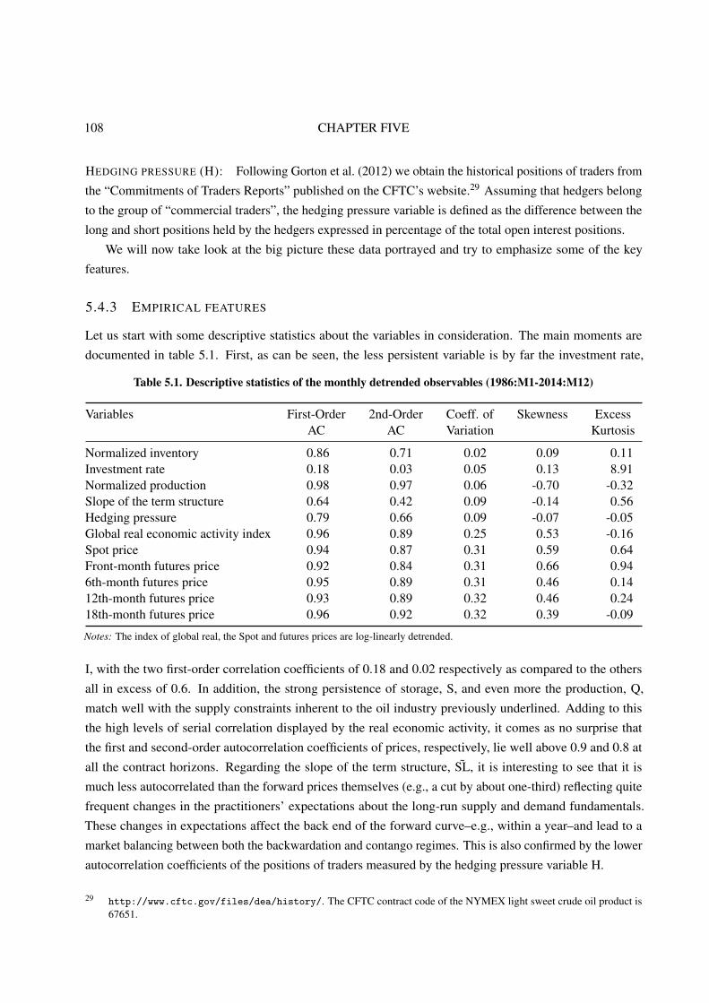
108 CHAPTER FIVE
HEDGING PRESSURE (H): Following Gorton et al. (2012) we obtain the historical positions of traders from
the “Commitments of Traders Reports” published on the CFTC’s website.29 Assuming that hedgers belong
to the group of “commercial traders”, the hedging pressure variable is defined as the difference between the
long and short positions held by the hedgers expressed in percentage of the total open interest positions.
We will now take look at the big picture these data portrayed and try to emphasize some of the key
features.
5.4.3 EMPIRICAL FEATURES
Let us start with some descriptive statistics about the variables in consideration. The main moments are
documented in table 5.1. First, as can be seen, the less persistent variable is by far the investment rate,
Table 5.1. Descriptive statistics of the monthly detrended observables (1986:M1-2014:M12)
Variables First-Order 2nd-Order Coeff. of Skewness ExcessAC AC Variation Kurtosis
Normalized inventory 0.86 0.71 0.02 0.09 0.11Investment rate 0.18 0.03 0.05 0.13 8.91Normalized production 0.98 0.97 0.06 -0.70 -0.32Slope of the term structure 0.64 0.42 0.09 -0.14 0.56Hedging pressure 0.79 0.66 0.09 -0.07 -0.05Global real economic activity index 0.96 0.89 0.25 0.53 -0.16Spot price 0.94 0.87 0.31 0.59 0.64Front-month futures price 0.92 0.84 0.31 0.66 0.946th-month futures price 0.95 0.89 0.31 0.46 0.1412th-month futures price 0.93 0.89 0.32 0.46 0.2418th-month futures price 0.96 0.92 0.32 0.39 -0.09
Notes: The index of global real, the Spot and futures prices are log-linearly detrended.
I, with the two first-order correlation coefficients of 0.18 and 0.02 respectively as compared to the others
all in excess of 0.6. In addition, the strong persistence of storage, S, and even more the production, Q,
match well with the supply constraints inherent to the oil industry previously underlined. Adding to this
the high levels of serial correlation displayed by the real economic activity, it comes as no surprise that
the first and second-order autocorrelation coefficients of prices, respectively, lie well above 0.9 and 0.8 at
all the contract horizons. Regarding the slope of the term structure, S̃L, it is interesting to see that it is
much less autocorrelated than the forward prices themselves (e.g., a cut by about one-third) reflecting quite
frequent changes in the practitioners’ expectations about the long-run supply and demand fundamentals.
These changes in expectations affect the back end of the forward curve–e.g., within a year–and lead to a
market balancing between both the backwardation and contango regimes. This is also confirmed by the lower
autocorrelation coefficients of the positions of traders measured by the hedging pressure variable H.
29 http://www.cftc.gov/files/dea/history/. The CFTC contract code of the NYMEX light sweet crude oil product is67651.
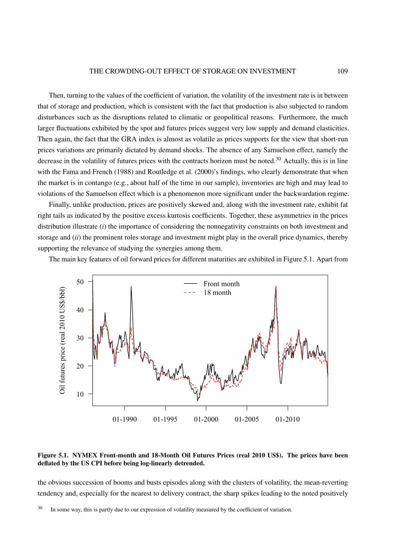
THE CROWDING-OUT EFFECT OF STORAGE ON INVESTMENT 109
Then, turning to the values of the coefficient of variation, the volatility of the investment rate is in between
that of storage and production, which is consistent with the fact that production is also subjected to random
disturbances such as the disruptions related to climatic or geopolitical reasons. Furthermore, the much
larger fluctuations exhibited by the spot and futures prices suggest very low supply and demand elasticities.
Then again, the fact that the GRA index is almost as volatile as prices supports for the view that short-run
prices variations are primarily dictated by demand shocks. The absence of any Samuelson effect, namely the
decrease in the volatility of futures prices with the contracts horizon must be noted.30 Actually, this is in line
with the Fama and French (1988) and Routledge et al. (2000)’s findings, who clearly demonstrate that when
the market is in contango (e.g., about half of the time in our sample), inventories are high and may lead to
violations of the Samuelson effect which is a phenomenon more significant under the backwardation regime.
Finally, unlike production, prices are positively skewed and, along with the investment rate, exhibit fat
right tails as indicated by the positive excess kurtosis coefficients. Together, these asymmetries in the prices
distribution illustrate (i) the importance of considering the nonnegativity constraints on both investment and
storage and (ii) the prominent roles storage and investment might play in the overall price dynamics, thereby
supporting the relevance of studying the synergies among them.
The main key features of oil forward prices for different maturities are exhibited in Figure 5.1. Apart from
10
20
30
40
50
Oil
fut
ures
pri
ce (
real
201
0 U
S$/
bbl)
Front month18 month
01-1990 01-1995 01-2000 01-2005 01-2010
Figure 5.1. NYMEX Front-month and 18-Month Oil Futures Prices (real 2010 US$). The prices have beendeflated by the US CPI before being log-linearly detrended.
the obvious succession of booms and busts episodes along with the clusters of volatility, the mean-reverting
tendency and, especially for the nearest to delivery contract, the sharp spikes leading to the noted positively
30 In some way, this is partly due to our expression of volatility measured by the coefficient of variation.
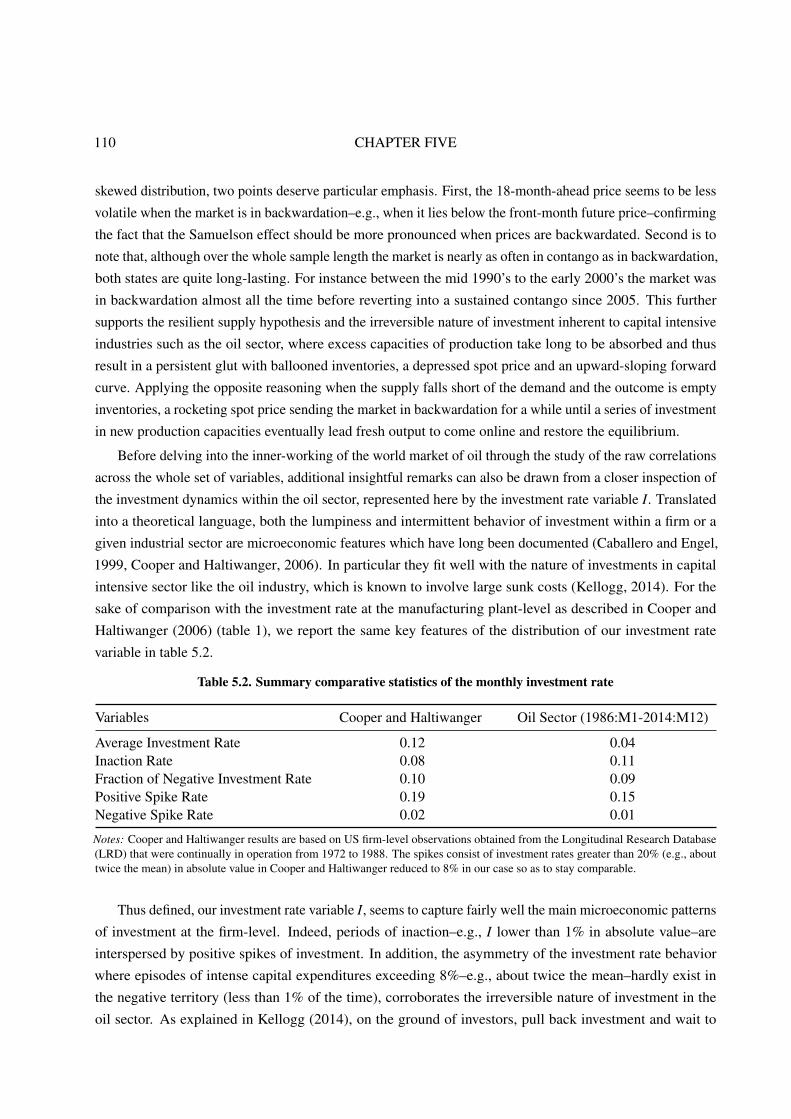
110 CHAPTER FIVE
skewed distribution, two points deserve particular emphasis. First, the 18-month-ahead price seems to be less
volatile when the market is in backwardation–e.g., when it lies below the front-month future price–confirming
the fact that the Samuelson effect should be more pronounced when prices are backwardated. Second is to
note that, although over the whole sample length the market is nearly as often in contango as in backwardation,
both states are quite long-lasting. For instance between the mid 1990’s to the early 2000’s the market was
in backwardation almost all the time before reverting into a sustained contango since 2005. This further
supports the resilient supply hypothesis and the irreversible nature of investment inherent to capital intensive
industries such as the oil sector, where excess capacities of production take long to be absorbed and thus
result in a persistent glut with ballooned inventories, a depressed spot price and an upward-sloping forward
curve. Applying the opposite reasoning when the supply falls short of the demand and the outcome is empty
inventories, a rocketing spot price sending the market in backwardation for a while until a series of investment
in new production capacities eventually lead fresh output to come online and restore the equilibrium.
Before delving into the inner-working of the world market of oil through the study of the raw correlations
across the whole set of variables, additional insightful remarks can also be drawn from a closer inspection of
the investment dynamics within the oil sector, represented here by the investment rate variable I. Translated
into a theoretical language, both the lumpiness and intermittent behavior of investment within a firm or a
given industrial sector are microeconomic features which have long been documented (Caballero and Engel,
1999, Cooper and Haltiwanger, 2006). In particular they fit well with the nature of investments in capital
intensive sector like the oil industry, which is known to involve large sunk costs (Kellogg, 2014). For the
sake of comparison with the investment rate at the manufacturing plant-level as described in Cooper and
Haltiwanger (2006) (table 1), we report the same key features of the distribution of our investment rate
variable in table 5.2.
Table 5.2. Summary comparative statistics of the monthly investment rate
Variables Cooper and Haltiwanger Oil Sector (1986:M1-2014:M12)
Average Investment Rate 0.12 0.04Inaction Rate 0.08 0.11Fraction of Negative Investment Rate 0.10 0.09Positive Spike Rate 0.19 0.15Negative Spike Rate 0.02 0.01
Notes: Cooper and Haltiwanger results are based on US firm-level observations obtained from the Longitudinal Research Database(LRD) that were continually in operation from 1972 to 1988. The spikes consist of investment rates greater than 20% (e.g., abouttwice the mean) in absolute value in Cooper and Haltiwanger reduced to 8% in our case so as to stay comparable.
Thus defined, our investment rate variable I, seems to capture fairly well the main microeconomic patterns
of investment at the firm-level. Indeed, periods of inaction–e.g., I lower than 1% in absolute value–are
interspersed by positive spikes of investment. In addition, the asymmetry of the investment rate behavior
where episodes of intense capital expenditures exceeding 8%–e.g., about twice the mean–hardly exist in
the negative territory (less than 1% of the time), corroborates the irreversible nature of investment in the
oil sector. As explained in Kellogg (2014), on the ground of investors, pull back investment and wait to
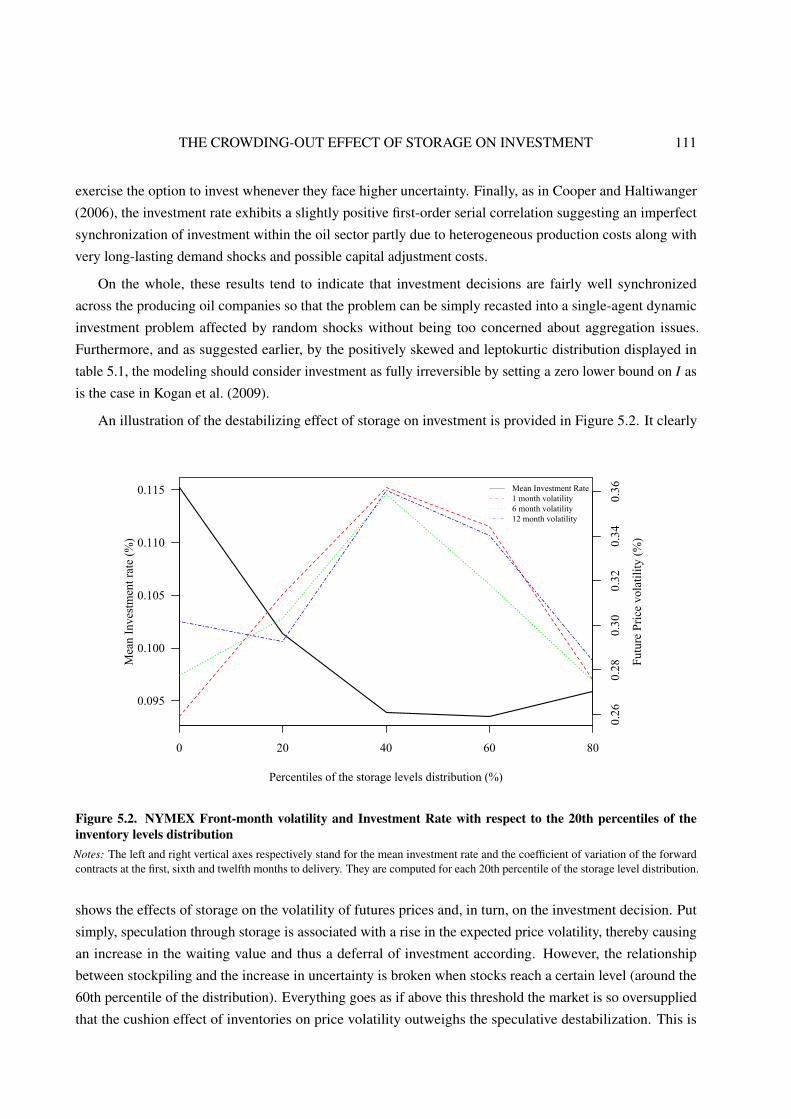
THE CROWDING-OUT EFFECT OF STORAGE ON INVESTMENT 111
exercise the option to invest whenever they face higher uncertainty. Finally, as in Cooper and Haltiwanger
(2006), the investment rate exhibits a slightly positive first-order serial correlation suggesting an imperfect
synchronization of investment within the oil sector partly due to heterogeneous production costs along with
very long-lasting demand shocks and possible capital adjustment costs.
On the whole, these results tend to indicate that investment decisions are fairly well synchronized
across the producing oil companies so that the problem can be simply recasted into a single-agent dynamic
investment problem affected by random shocks without being too concerned about aggregation issues.
Furthermore, and as suggested earlier, by the positively skewed and leptokurtic distribution displayed in
table 5.1, the modeling should consider investment as fully irreversible by setting a zero lower bound on I as
is the case in Kogan et al. (2009).
An illustration of the destabilizing effect of storage on investment is provided in Figure 5.2. It clearly
0 20 40 60 80
0.095
0.100
0.105
0.110
0.115
Percentiles of the storage levels distribution (%)
Mea
n In
vest
men
t rat
e (%
)
0.26
0.28
0.30
0.32
0.34
0.36
Fut
ure
Pri
ce v
olat
ilit
y (%
)
Mean Investment Rate1 month volatility6 month volatility12 month volatility
Figure 5.2. NYMEX Front-month volatility and Investment Rate with respect to the 20th percentiles of theinventory levels distributionNotes: The left and right vertical axes respectively stand for the mean investment rate and the coefficient of variation of the forwardcontracts at the first, sixth and twelfth months to delivery. They are computed for each 20th percentile of the storage level distribution.
shows the effects of storage on the volatility of futures prices and, in turn, on the investment decision. Put
simply, speculation through storage is associated with a rise in the expected price volatility, thereby causing
an increase in the waiting value and thus a deferral of investment according. However, the relationship
between stockpiling and the increase in uncertainty is broken when stocks reach a certain level (around the
60th percentile of the distribution). Everything goes as if above this threshold the market is so oversupplied
that the cushion effect of inventories on price volatility outweighs the speculative destabilization. This is
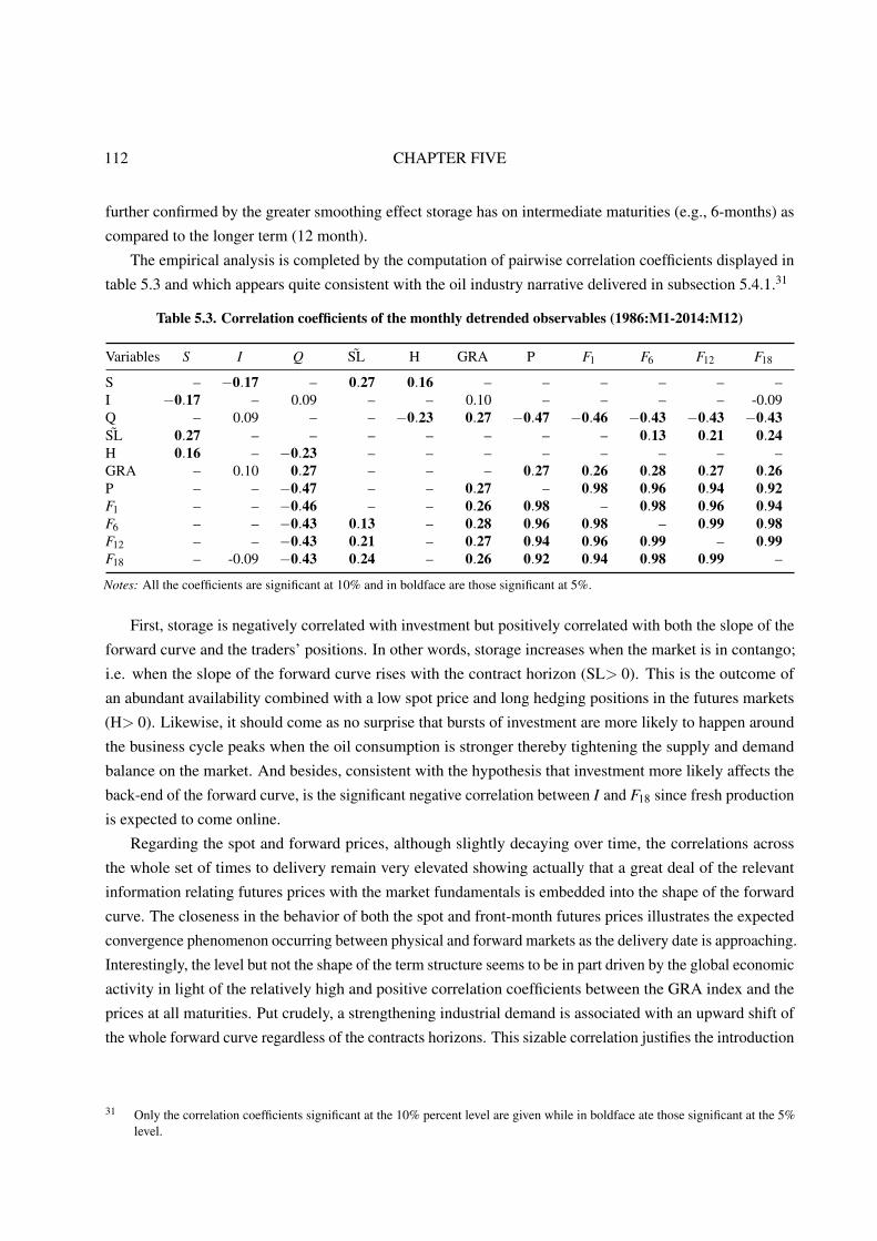
112 CHAPTER FIVE
further confirmed by the greater smoothing effect storage has on intermediate maturities (e.g., 6-months) as
compared to the longer term (12 month).
The empirical analysis is completed by the computation of pairwise correlation coefficients displayed in
table 5.3 and which appears quite consistent with the oil industry narrative delivered in subsection 5.4.1.31
Table 5.3. Correlation coefficients of the monthly detrended observables (1986:M1-2014:M12)
Variables S I Q S̃L H GRA P F1 F6 F12 F18
S – −0.17 – 0.27 0.16 – – – – – –I −0.17 – 0.09 – – 0.10 – – – – -0.09Q – 0.09 – – −0.23 0.27 −0.47 −0.46 −0.43 −0.43 −0.43S̃L 0.27 – – – – – – – 0.13 0.21 0.24H 0.16 – −0.23 – – – – – – – –GRA – 0.10 0.27 – – – 0.27 0.26 0.28 0.27 0.26P – – −0.47 – – 0.27 – 0.98 0.96 0.94 0.92F1 – – −0.46 – – 0.26 0.98 – 0.98 0.96 0.94F6 – – −0.43 0.13 – 0.28 0.96 0.98 – 0.99 0.98F12 – – −0.43 0.21 – 0.27 0.94 0.96 0.99 – 0.99F18 – -0.09 −0.43 0.24 – 0.26 0.92 0.94 0.98 0.99 –
Notes: All the coefficients are significant at 10% and in boldface are those significant at 5%.
First, storage is negatively correlated with investment but positively correlated with both the slope of the
forward curve and the traders’ positions. In other words, storage increases when the market is in contango;
i.e. when the slope of the forward curve rises with the contract horizon (SL> 0). This is the outcome of
an abundant availability combined with a low spot price and long hedging positions in the futures markets
(H> 0). Likewise, it should come as no surprise that bursts of investment are more likely to happen around
the business cycle peaks when the oil consumption is stronger thereby tightening the supply and demand
balance on the market. And besides, consistent with the hypothesis that investment more likely affects the
back-end of the forward curve, is the significant negative correlation between I and F18 since fresh production
is expected to come online.
Regarding the spot and forward prices, although slightly decaying over time, the correlations across
the whole set of times to delivery remain very elevated showing actually that a great deal of the relevant
information relating futures prices with the market fundamentals is embedded into the shape of the forward
curve. The closeness in the behavior of both the spot and front-month futures prices illustrates the expected
convergence phenomenon occurring between physical and forward markets as the delivery date is approaching.
Interestingly, the level but not the shape of the term structure seems to be in part driven by the global economic
activity in light of the relatively high and positive correlation coefficients between the GRA index and the
prices at all maturities. Put crudely, a strengthening industrial demand is associated with an upward shift of
the whole forward curve regardless of the contracts horizons. This sizable correlation justifies the introduction
31 Only the correlation coefficients significant at the 10% percent level are given while in boldface ate those significant at the 5%level.

THE CROWDING-OUT EFFECT OF STORAGE ON INVESTMENT 113
of a persistent demand factor as in Routledge et al. (2000) to account for such an underlying consumption
growth engine which puts pressure on the supply side.
Nevertheless, further points deserve some comments, as one might be puzzled in view of the absence
of significant relationships found in the true data such as those between storage and prices at all times to
maturity. A possible explanation is that WTI futures contracts exchanged on the NYMEX better reflect the
contemporaneous supply and demand conditions in the US than elsewhere in the world.32 Another reason
has to do with the typical lack of reliability of data on quantities in general and on inventories in particular.
Hidden strategic state-owned stocks added to substantial floating storage are among the factors prone to
make difficult the precise assessment of inventory levels at the global scale. Having said this, the significant
contemporaneous correlations between the production and futures prices qualify somewhat the disappointing
weak correlations results as production is known to be much more precisely estimated than storage. Some
authors like Gorton et al. (2012) decide to lag the data to account for some possible reporting time. Because
of the lack of true theoretical justification for introducing such lags in the variables, and given the strong and
consistent contemporaneous correlations observed between production and prices as well as between the
slope of the term structure with storage,33 we instead prefer not to try adding some hypothetical lags in the
variables and to be content with the overall coherent, albeit imperfect, picture delivered by the correlations
table.
In light of these results, the subsequent modeling must be able to generate endogenously and alternatively
backwardation and contango states. Conjointly, these states must be accompanied by lumpy and intermittent
episodes of investment and complement the storage activity, which is no longer profitable whenever production
capacities falls short of the industrial demand, especially during economic booms. Indeed the relative
abundance in the market goes hand-in-hand with (i) a bearish market poorly encouraging investment but
rather much more inclined to support the accumulation of inventories by speculators willing to make the
most of the resulting low spot price, (ii) a forward market in contango in response to the net-long positions of
refiners hedging their future crude supply by buying forwards contracts, (iii) steeper fluctuations of the futures
prices, since linked to the spot price through the arbitrage equation, thus leading to a very uncertain economic
environment favorable to speculative storage while increasing the option value to delay investment. To what
extent these stylized facts can be reproduced by embedding the speculative storage within the standard capital
accumulation model with an irreversible constraint on investment is the topic further studied in the remainder
of the chapter.
32 Unsurprisingly if, as in most empirical studies using the crude stocks data, when the more reliable US instead of world levelsof inventories are used the correlation between spot prices and stocks is -0.10 and significant at 10%.
33 These variables are reliable indicators of the state of the market fundamentals.
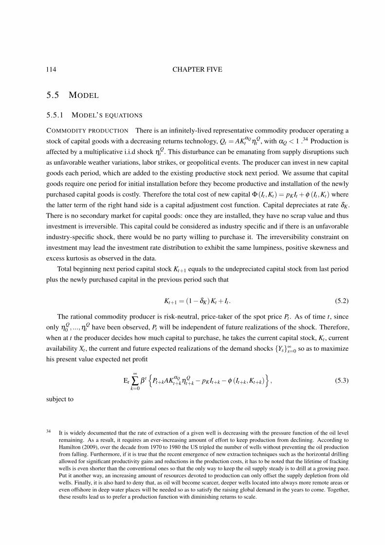
114 CHAPTER FIVE
5.5 MODEL
5.5.1 MODEL’S EQUATIONS
COMMODITY PRODUCTION There is an infinitely-lived representative commodity producer operating a
stock of capital goods with a decreasing returns technology, Qt = AKαQt η
Qt , with αQ < 1 .34 Production is
affected by a multiplicative i.i.d shock ηQt . This disturbance can be emanating from supply disruptions such
as unfavorable weather variations, labor strikes, or geopolitical events. The producer can invest in new capital
goods each period, which are added to the existing productive stock next period. We assume that capital
goods require one period for initial installation before they become productive and installation of the newly
purchased capital goods is costly. Therefore the total cost of new capital Φ(It ,Kt) = pKIt +φ (It ,Kt) where
the latter term of the right hand side is a capital adjustment cost function. Capital depreciates at rate δK .
There is no secondary market for capital goods: once they are installed, they have no scrap value and thus
investment is irreversible. This capital could be considered as industry specific and if there is an unfavorable
industry-specific shock, there would be no party willing to purchase it. The irreversibility constraint on
investment may lead the investment rate distribution to exhibit the same lumpiness, positive skewness and
excess kurtosis as observed in the data.
Total beginning next period capital stock Kt+1 equals to the undepreciated capital stock from last period
plus the newly purchased capital in the previous period such that
Kt+1 = (1−δK)Kt + It . (5.2)
The rational commodity producer is risk-neutral, price-taker of the spot price Pt . As of time t, since
only ηQ0 , ...,η
Qt have been observed, Pt will be independent of future realizations of the shock. Therefore,
when at t the producer decides how much capital to purchase, he takes the current capital stock, Kt , current
availability Xt , the current and future expected realizations of the demand shocks {Ys}∞s=0 so as to maximize
his present value expected net profit
Et
∞
∑k=0
βt{
Pt+kAKαQt+kη
Qt+k− pKIt+k−φ (It+k,Kt+k)
}, (5.3)
subject to
34 It is widely documented that the rate of extraction of a given well is decreasing with the pressure function of the oil levelremaining. As a result, it requires an ever-increasing amount of effort to keep production from declining. According toHamilton (2009), over the decade from 1970 to 1980 the US tripled the number of wells without preventing the oil productionfrom falling. Furthermore, if it is true that the recent emergence of new extraction techniques such as the horizontal drillingallowed for significant productivity gains and reductions in the production costs, it has to be noted that the lifetime of frackingwells is even shorter than the conventional ones so that the only way to keep the oil supply steady is to drill at a growing pace.Put it another way, an increasing amount of resources devoted to production can only offset the supply depletion from oldwells. Finally, it is also hard to deny that, as oil will become scarcer, deeper wells located into always more remote areas oreven offshore in deep water places will be needed so as to satisfy the raising global demand in the years to come. Together,these results lead us to prefer a production function with diminishing returns to scale.
THE CROWDING-OUT EFFECT OF STORAGE ON INVESTMENT 115
Kt+1 = (1−δK)Kt + It .
It ≥ 0.(5.4)
THE STORAGE DEMAND In addition to producers and consumers, the commodity market comprises storers
also assumed rational, risk-neutral and price-takers. Through the storage technology, the commodity is
transferred from one period to another at a constant marginal cost k. Storers maximize the expected net profit
from purchasing St of the commodity and selling it next period,
maxSt≥0
[(1−δS)β Et Pt+1−Pt − k]St , (5.5)
with δS the decay rate of inventories. The total availability of the commodity Xt is determined by the sum of
the current supply of the commodity, Qt , and the inventories inherited from the previous period net of the
share lost due to decay, that is
Xt = Qt +(1−δS)St−1. (5.6)
MARKET CLEARING The market demand for the commodity constitutes the consumption demand D(Pt)
and the speculative demand for storage St . In each period, the market clears for a spot price Pt when the
availability equals total demand according to the equilibrium condition
Xt = D(Pt)+St , (5.7)
with the linear demand function D(Pt), assumed downward-sloping in Pt and subject to a multiplicative
stochastic disturbance Yt described by an autoregressive process.35 Hence, the linear demand function takes
the following form:
D(Pt) = D̄(
1+αD
P̄(Pt − P̄)
)Yt , (5.8)
where D̄ and P̄ represent the steady-state values of final demand and the spot price respectively and αD is the
elasticity of demand.
5.5.2 THE COMPETITIVE EQUILIBRIUM
Definition 1. A rational competitive equilibrium is given by the path of capital investment {It}∞s=0, storage
{St}∞s=0 and prices {Pt}∞
s=0 such that: (i) the representative producer maximizes the present value of his
expected net profits subject to the sequence of capital accumulation constraints in (5.4); (ii) storers maximize
the present value of their net profits subject to the nonnegativity constraint on storage; and (iii) the market
clears in every period.
35 The demand shock is an AR(1) process: Yt = ρYt−1 +ηQt . The demand uncertainty is modeled as a persistent stochastic
process akin to the cyclical fluctuations of the international business cycle.
116 CHAPTER FIVE
Before deriving the model’s first order conditions another assumption will be made regarding the
convex adjustment costs Φ. Even though the observed investment rate exhibits a slightly positive serial
correlation which might call for some kind of convex adjustment costs, we believe they matter less than the
irreversibility constraint on I and so can be overlooked without changing neither the internal relationships
among the variables nor the qualitative nature of the dynamics implied by the model.36 Hence, for the sake of
simplification, φ (It ,Kt) in equation (5.3) is set to zero in the rest of the chapter. Taking the price of capital pK
as a constant and fixed at 1, it turns out that the producer’s maximization problem given by the equations (5.3)
and (5.4) delivers the following Euler equation:
β Et
{Pt+1αQ
(AKαQ−1
t+1 ηQt+1
)+(1−δK)
}≤ 1, = 1 if It > 0. (5.9)
The investment decision rests on the present value of the expected marginal return on capital, the left hand
side of equation (5.9) being equal to its marginal cost. Should the right hand exceed the left, there is a large
enough opportunity cost of investing today which makes the investment in the current period non-viable.
Likewise, regarding the speculative demand for storage, differentiating (5.5) with respect to St ≥ 0 yields
the following storer’s optimality condition:
β (1−δS)Et Pt+1−Pt − k ≤ 0, = 0 if St > 0. (5.10)
The storage decision hinges on whether the commodity price (net of the carrying costs) grows at the rate
of interest. It is profitable to store only if the price growth rate equals the interest rate. Therefore, a market
in contango is one in which the expected price would rise at the decay adjusted interest rate. Finally, as a
result of the rational expectations assumption, both the investment and storage are forward-looking decisions
resting on the expectations agents forms regarding the sole next-period price F1 without any consideration for
F2 and the subsequent forward prices.
5.5.3 NUMERICAL SOLUTION
The nonlinear nature of the decisions rules warrants the use of global numerical solution methods. We
choose to employ a projection method to approximate the solution of our model. There are two endogenous
state variables Kt ,Xt , and one stochastic state variable Yt . The decision variables are St and It , while Pt falls
from the market clearing condition. P is regarded as an additional control variable and so are the futures
prices. To solve the model, the state space is discretized and the bounds are defined around the steady state
values of the state variables. It thus consists in [X ,X ]× [K,K]× [Y ,Y ]. The solution to the time iteration
problem delivers three time-invariant policy functions P = P (X ,K,Y ), I = I (X ,K,Y ), S = S (X ,K,Y ).
These policy functions solve the constrained system of equations (5.7) and (5.9)-(5.10), using the transition
36 The presence of convex adjustment costs will result in a zero-lower bound less often binding thereby leading to a smoother,more persistent and symmetric distribution rate of investment.
THE CROWDING-OUT EFFECT OF STORAGE ON INVESTMENT 117
equations in (5.4) and (5.6) to bring the model forward.37 The model solution yields nonlinear decision rules
that are governed by endogenous thresholds, which in turn depend on the state variables. In order to assess
the extent to which storage interacts with the irreversibility constraint on investment, we proceed by studying
two models, identically calibrated and which differ only by whether there is the possibility for storage.
5.6 SIMULATION RESULTS
In this section, we will discuss simulation results of two models: a baseline irreversible investment model
and the same basic set-up but augmented with storage capacity. The former is no different from the model set
out in the previous section except that we remove the possibility of stockpiling.
5.6.1 CALIBRATION
In calibrating the models, if the choices have been largely guided by the above empirical analysis, a particular
attention has been also paid to their internal consistency as it is a connection between two strands of literature
mostly developed independently of one another. The calibrated parameter values are reported in table 5.4
and are selected so as to follow the standard calibration and, when available, estimation results found in the
investment and storage literature. The share of capital αK is set to 0.33 which is equivalent to a long-run
supply elasticity of αK/(1−αK
)≈ 0.5. Since no distinction is drawn between short and long-run demand
elasticities, αD is set to −0.1, a value in the range of estimates provided in Dahl (1993) and Cooper (2003)
and also reflecting the lack of substitutes for such a basic product. It has to be said that these low values of
supply and demand responsiveness have been further suggested by the substantial gap in volatility between
the prices and quantities noted in Table 5.1. The depreciation rate of capital δK is set to 10% which is
intermediate in the typical range of 8 and 12% used in the related literature (Kogan et al., 2009, Kung and
Schmid, 2015). Likewise, the decay rate on storage δS is fixed at 5% to be consistent with the 3% used in
Routledge et al. (2000). We decided to also account for a physical storage cost, k = 5%, unlike most of the
empirical studies of the storage model, which specify either a proportional cost as in Deaton and Laroque
(1996) or a constant marginal storage cost following Cafiero et al. (2011b). The relatively low selected
value–e.g., 1% of the long-run average price–reflects this modeling choice, as we want to avoid precluding
storage with too high a total cost of carry. Regarding the demand shock Y , its role in the model’s internal
mechanics is very close in nature to the one played by the income shock variable embedded in the storage
framework developed in Dvir and Rogoff (2009, 2014). Hence, for the persistence value of the demand shock
ρ , we borrow the value they used which is equal to 0.5. Lastly, the volatilites of supply and demand shocks
are chosen so as to match the observed coefficient of variation of production (table 5.1).38 Before running
37 The model is solved by implementing policy function iteration using cubic spline function approximation through "RationalExpectations Complementarity Solver" (RECS) developed by Gouel (2013b) and available from the following websitehttp://www.recs-solver.org//.
38 As the consumption simply equals the difference between the production and the stock variation, its descriptive statistics havenot been documented in table 5.1. Still, the coefficient of variation of the normalized demand, equals to 0.0632, is really similarto the production’s one and thus to the selected value of 0.05.
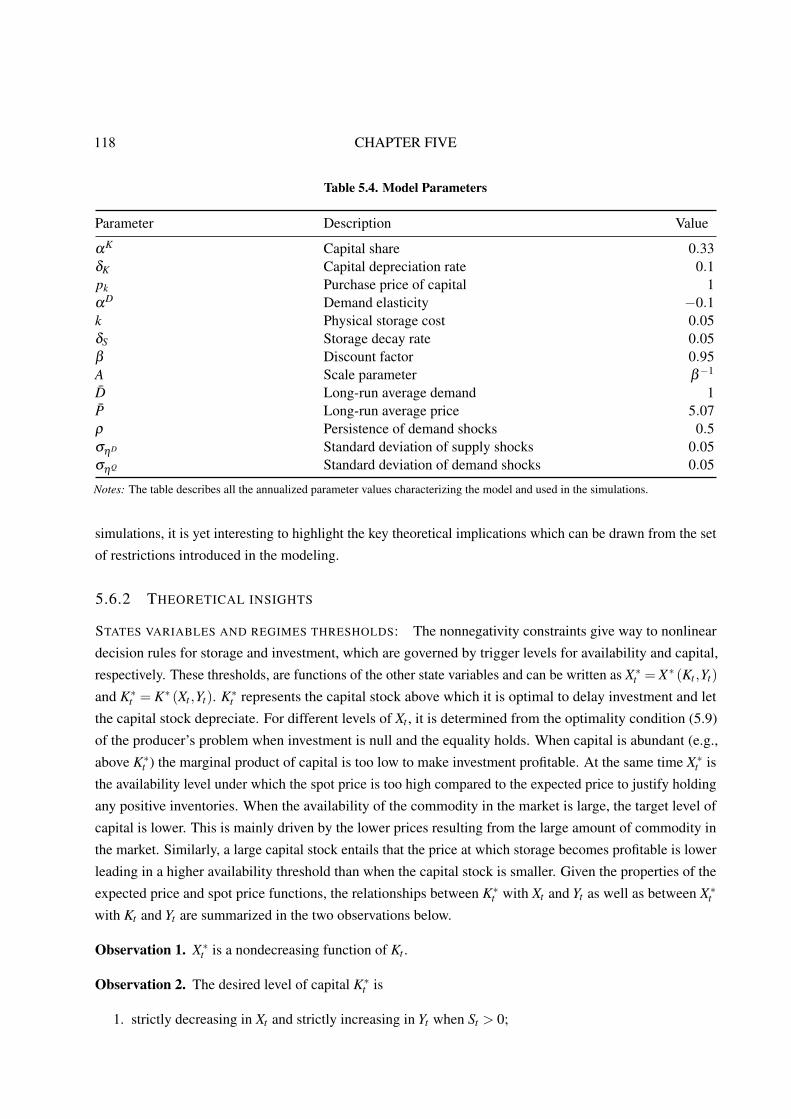
118 CHAPTER FIVE
Table 5.4. Model Parameters
Parameter Description Value
αK Capital share 0.33δK Capital depreciation rate 0.1pk Purchase price of capital 1αD Demand elasticity −0.1k Physical storage cost 0.05δS Storage decay rate 0.05β Discount factor 0.95A Scale parameter β−1
D̄ Long-run average demand 1P̄ Long-run average price 5.07ρ Persistence of demand shocks 0.5σηD Standard deviation of supply shocks 0.05σηQ Standard deviation of demand shocks 0.05
Notes: The table describes all the annualized parameter values characterizing the model and used in the simulations.
simulations, it is yet interesting to highlight the key theoretical implications which can be drawn from the set
of restrictions introduced in the modeling.
5.6.2 THEORETICAL INSIGHTS
STATES VARIABLES AND REGIMES THRESHOLDS: The nonnegativity constraints give way to nonlinear
decision rules for storage and investment, which are governed by trigger levels for availability and capital,
respectively. These thresholds, are functions of the other state variables and can be written as X∗t = X∗ (Kt ,Yt)
and K∗t = K∗ (Xt ,Yt). K∗t represents the capital stock above which it is optimal to delay investment and let
the capital stock depreciate. For different levels of Xt , it is determined from the optimality condition (5.9)
of the producer’s problem when investment is null and the equality holds. When capital is abundant (e.g.,
above K∗t ) the marginal product of capital is too low to make investment profitable. At the same time X∗t is
the availability level under which the spot price is too high compared to the expected price to justify holding
any positive inventories. When the availability of the commodity in the market is large, the target level of
capital is lower. This is mainly driven by the lower prices resulting from the large amount of commodity in
the market. Similarly, a large capital stock entails that the price at which storage becomes profitable is lower
leading in a higher availability threshold than when the capital stock is smaller. Given the properties of the
expected price and spot price functions, the relationships between K∗t with Xt and Yt as well as between X∗twith Kt and Yt are summarized in the two observations below.
Observation 1. X∗t is a nondecreasing function of Kt .
Observation 2. The desired level of capital K∗t is
1. strictly decreasing in Xt and strictly increasing in Yt when St > 0;
THE CROWDING-OUT EFFECT OF STORAGE ON INVESTMENT 119
2. increasing with Yt and invariant to Xt when St = 0.
First, looking at the impact of capital on the availability threshold X∗ under which stocks are empty,
observation 1 simply shows that a greater capital level is associated with a higher expected supply weighing
on any increase of the expected price.
Then, switching to the effects of availability on the target capital level K∗, two distinct regimes must
be explored. With this in mind, the first statement in observation 2 corresponds to the case when inventory
building is profitable, that is St > 0. The interpretation is straightforward recalling from the arbitrage
equation (5.10) that Et Pt+1 = β (1−δS)−1 (P (Xt ,Kt ,Yt)+ k), which implies that variations in spot and
expected prices are coupled. Hence, since the expected price is a decreasing function of the availability in
the market, when the commodity is abundant and storage is positive the expected price is low. This in turn
reduces the net marginal benefit from investment and in the end lowers the desired level of capital. The
result points to the first source of divergence between the two models with and without storage. Put simply,
storage increases the value of postponing investment by lowering the cut off value above which it is optimal
to delay capital expenditures. In addition, and perhaps even more importantly, by inducing conditional
heteroskedasticity in prices the storage mechanism implies a higher uncertainty around the expected price
which both supports speculation and heightens the option value of deferring investment. Through these
two channels, the presence of storage has a crowding out effect on investment. The outcome is a gradual
shrinkage of the productive capacity accompanied by withdrawals of inventories eventually making the
occurrence of a stockout more and more likely.
Finally, once the supply falls short of the demand, stocks are sold out–e.g.,St = 0–and from (5.10)
Et Pt+1 = Et[D−1 (Qt+1,Yt+1)
]. In other words, the expected price is no longer a function of the spot price.
The stockout regime reverts to the model of irreversible investment without inventory building capacity, in
which the desired capital level is a function of the realized supply-side shock, the steady state values of the
price and consumption demand of the commodity. The realized shock Yt raises the trigger value of capital.
To borrow the terminology from the option pricing literature, the value of waiting to invest is lower when the
realized value of the disturbance is high. Indeed, given the assumed persistence of shocks to the consumption
demand for the commodity, the whole conditional distribution F (Yt+1|Yt) shifts to the right giving greater
probability to larger Yt+1 values, thereby rendering the opportunity to invest and to terminate the option more
attractive than waiting. Then again, this investment incentive is further strengthened by what can be called
the “uncertainty effect”. The reason is that, if the high spot price deters inventory speculation, it also provides
a much kinder environment for investing since the expected price, now decoupled from the very volatile spot
price, is more stable and even smoothed out according to the Samuelson effect. The volatility of the expected
price is now constant since the expected price itself is a function the capital stock and the expected demand
shock.39
All in all, the combination of persistent demand shocks and time-variations in both the desired level of
capital and uncertainty of future price are the key reasons behind the certain substituability, albeit imperfect,
between storage and investment.
39 The constant volatility of the expected price in a stockout regime is discussed in Deaton and Laroque (1992, 1996).
120 CHAPTER FIVE
Together, both zero-lower bounds on storage and investment split the state space into four regions
demarcated by the capital and availability thresholds determined by the current supply and demand conditions.
They are described in the following observation:
Observation 3. The competitive equilibrium can be characterized by four regimes:
1. It = 0, St = 0, if Kt ≥ K∗t and Xt ≤ X∗t ;
2. It = 0, St > 0, if Kt ≥ K∗t and Xt > X∗t ;
3. It > 0, St = 0, if Kt < K∗t and Xt ≤ X∗t ;
4. It > 0, St > 0, if Kt < K∗t and Xt > X∗t .
If both I = 0 and S = 0, the expected price is only a function of expected production, which is constant
AKαt . This is a regime where the economy has overcapacities of production and it is optimal to defer
investment. Furthermore, in spite of a relatively low spot price, it is not profitable to store neither because of
the large productive capacity. Indeed, as stated in observation 1 the very high capital level weighs on the
expected price, preventing the latter from rising sufficiently so as to cover the purchasing and carrying cost of
inventories.
If only I = 0, there is still an excess of capital but not enough to preclude expected price from increasing
so that it becomes profitable to stockpile (e.g., S > 0). So long as the expected commodity price grows at a
higher rate than the rate of interest (net of decay), it is profitable to store.
If now S = 0 but I > 0, the market is tight resulting in a high spot price. Futures market is backwardated
and selling inventories today is optimal. Although the availability is too scarce to allow storage, the associated
environment of high prices encourages investment to reach the optimal level of capital K∗.
Finally, as mentioned previously the investment-storage substituability is only partial and it might be
the case that it is optimal to invest and store jointly so that I > 0, S > 0. It has to be noted that, in this
regime, both the S and I values are much lower than those reached when one of the constraint is binding. The
market equilibrium can enter this regime for instance if, despite a capital level lying below the desired K∗, a
high positive value of the supply shock ηQ yields an availability in excess of the threshold X∗. The latter
scenario is even more likely if supplemented by a persistent low demand state Y which will lower X∗ while
raising K∗. The outcome is a relatively slack market in which inventories are used to absorb excess supply.
Yet, and contrary to the first regime when I = 0 and S = 0, here the stock of capital is not large and so (i)
is not pressing down the expected price increase needed to cover the carrying cost of inventories, (ii) it is
still optimal to invest and bring the capital stock to the target K∗. Moreover, the quantities S at stake being
lower than they are when investment is stuck at its zero-lower bound, they have too limited an impact on the
expected price volatility to make very attractive the option value of waiting.
Let us move now to the characterization of the policy functions prevailing in the various market regimes.

THE CROWDING-OUT EFFECT OF STORAGE ON INVESTMENT 121
0.8 0.9 1 1.1 1.2 1.3 1.4 1.5X
0
1
2
3
4
5
6
7
8
9
10
P
D!1(X) !
# P (Kmin; 7Y )
" P (Kmax; 7Y )
Figure 5.3. Price FunctionNotes: Two price functions, obtained for the highest and the lowest capital levels, are plotted against different levels of availability X .Additionally, the inverse demand function that prevails when inventories are null is plotted in the dashed line.
POLICY FUNCTIONS’ BEHAVIORS X∗ threshold point implies that the price function is nonlinear and
follows a two regime equilibrium which, from equation (5.10), can be written as:
Pt = P (Xt ,Kt ,Yt) =
β (1−δS)Et{Pt+1}− k if Xt > X∗t
D−1(Xt) otherwise.(5.11)
The rule can be summarized in the following functional form:
P (Xt ,Kt ,Yt) = max[β (1−δS)Et Pt+1− k,D−1 (Xt)
]. (5.12)
Figure 5.3 depicts the two regimes of the price policy function with respect to the availability and for two
extreme values of K. The abscissa of the kink is X∗ below which inventories are zero. As a result, the spot
price is only function of the consumption demand assumed linear. In line with observation 1, a high level
of capital is associated with a right shift of X∗. Where there is a large productive capacity, the spot price is
lower for all levels of availability and storage becomes optimal at a higher availability level. Characterizing
P (Xt ,Kt ,Yt) in terms of the quadrants shaped by X∗t and K∗t gives:

122 CHAPTER FIVE
Observation 4. The equilibrium price function P (Xt ,Kt ,Yt) relates to different levels of capital and avail-
ability in the following manner :
1. P (Xt ,Kt ,Yt) is strictly decreasing in Xt ;
2. P (Xt ,Kt ,Yt) is nonincreasing in Kt .
The first part of the observation is obvious and does not deserve additional comments. Regarding the
second point, the associated explanation is actually rather intuitive. Knowing that when inventories are carried
over, the price function is linked to the behavior of the expected price along the capital stock dimension.
Since the equilibrium of the model is described in terms of a desired level of capital K∗, the expected price is
also a function of this threshold. Specifically, when the capital stock lies below K∗, investment is positive and
brings back the next period capital stock to its optimal level. In this regime, the expected price is disconnected
from the level of capital and so is the current spot price.
On the other hand, when the capital stock is above K∗, there is no investment and the next period capital
stock equals the current capital stock less depreciation. Since a high level of capital entails a high expected
supply, it turns out that the expected price and the spot price are decreasing in the capital stock whenever its
current value exceeds K∗. Consequently, whether K is below or above K∗, the spot price is either independent
or a decreasing function of the capital stock.
The same characterization can be derived for the other two investment and storage policy functions.
Observation 5. The equilibrium investment and storage functions, It = I (Xt ,Kt ,Yt) and St = S (Xt ,Kt ,Yt),
relate to availability, capital and demand shock in the following manner :
1. I (Xt ,Kt ,Yt) is nonincreasing in Xt and Kt and increasing in Yt ;
2. S (Xt ,Kt ,Yt) is nondecreasing in Xt , nonincreasing in Kt , and decreasing in Yt .
The observation is further illustrated in Figure 5.4 exhibiting the investment and storage functions as they
relate to the state variables, X , K, and Y . The substituability between investment and storage as well as the
nonlinearities embedded in this model are well represented by these functions and the different kinks at the
thresholds, X∗ and K∗, can be identified.
As can be seen on the left panel, when X < X∗, I is constant with respect to availability and decreasing
with K. The reason is that the investment decision is driven by the expected price. Below X∗, the relationship
between the expected and spot price is severed. In a stockout market, the expected price only depends on the
next period stock of capital along with the expected state of the demand governed by the autocorrelated shock
Y . Investment follows suit: for a given fixed capital stock lying below K∗, optimal investment is constant and
equals the gap between K and its target K∗ so as to restore the optimality. Therefore, the higher K the lower I.
In sum, whether K exceeds its target, I is either null or decreasing in K.
On the other hand, when the commodity is abundant in the market so that X lies above X∗, I is decreasing
in X . In this regime, as the storage arbitrage condition holds, the expected price is indeed a function of the
spot price which is decreasing with the availability. Moreover, given that each period the market availability

THE CROWDING-OUT EFFECT OF STORAGE ON INVESTMENT 123
0.6 0.8 1 1.2 1.4Availability
0
0.05
0.1
0.15
0.2
0.25
0.3
0.35
0.4
0.45
0.5
Inve
stm
ent,
Sto
rage
a) Decision rules and the capital stock
S (KL; 7Y )
S (KH ; 7Y )
I (KH ; 7Y )
I (KL; 7Y )
0.6 0.8 1 1.2 1.4Availability
0
0.05
0.1
0.15
0.2
0.25
0.3
0.35
0.4
0.45
0.5b) Decision rules and demand shocks
S ( 7K;YL)
S ( 7K;YH)
I ( 7K;YH)
I ( 7K;YL)
Figure 5.4. Investment and Storage FunctionsNotes: The investment and storage functions for the highest and lowest value of capital and demand shock are plotted againstdifferent levels of volatility. Panel a) represents the two nonlinear functions in terms of the two extreme values of capital. Panel b)represents the functions for the two extreme realizations of the demand shock.
equals the sum of past inventories with the realized production, an increase in the productive capacity is
sluggish whenever stockpiling is optimal. It must be added that the rise in the option value of waiting stems
from the higher uncertainty inherent in the transmission of spot price volatility to the expected price. It turns
out that the bigger the quantity in store, the greater the crowing-out effect on investment which, consequently,
is a nonincreasing function of availability for any given level of capital.
For its part, storage is nondecreasing in X and Y . Storage is profitable only when the commodity is
sufficiently abundant in the market so as to depress the spot price. Investment and storage are negatively
correlated, with inventories standing high when the market is flooded. Since excess supply is persistent, as
the constant gradual shrinkage of the capital stock is slow, storage becomes more important as an adjustment
channel while the productive capacity adjusts. Therefore, storage does not vary much with the capital stock.
As already mentioned and illustrated in the panel b) of figure 5.4, investment and, interestingly storage
too, are really reactive to demand shocks. Investment response is of the same order of magnitude. All that
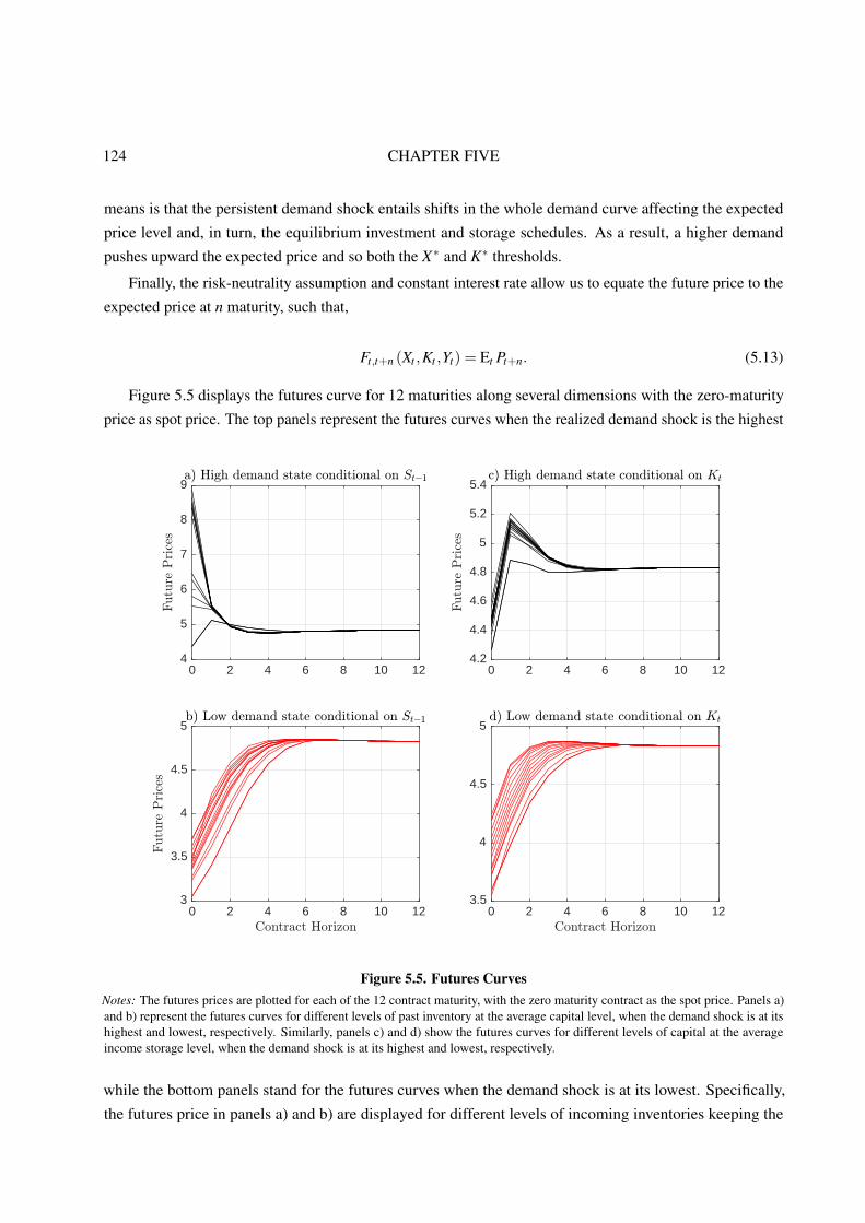
124 CHAPTER FIVE
means is that the persistent demand shock entails shifts in the whole demand curve affecting the expected
price level and, in turn, the equilibrium investment and storage schedules. As a result, a higher demand
pushes upward the expected price and so both the X∗ and K∗ thresholds.
Finally, the risk-neutrality assumption and constant interest rate allow us to equate the future price to the
expected price at n maturity, such that,
Ft,t+n (Xt ,Kt ,Yt) = Et Pt+n. (5.13)
Figure 5.5 displays the futures curve for 12 maturities along several dimensions with the zero-maturity
price as spot price. The top panels represent the futures curves when the realized demand shock is the highest
0 2 4 6 8 10 124
5
6
7
8
9
Futu
rePrice
s
a) High demand state conditional on St!1
0 2 4 6 8 10 12Contract Horizon
3
3.5
4
4.5
5
Futu
rePrice
s
b) Low demand state conditional on St!1
0 2 4 6 8 10 124.2
4.4
4.6
4.8
5
5.2
5.4
Futu
rePrice
s
c) High demand state conditional on Kt
0 2 4 6 8 10 12Contract Horizon
3.5
4
4.5
5d) Low demand state conditional on Kt
Figure 5.5. Futures CurvesNotes: The futures prices are plotted for each of the 12 contract maturity, with the zero maturity contract as the spot price. Panels a)and b) represent the futures curves for different levels of past inventory at the average capital level, when the demand shock is at itshighest and lowest, respectively. Similarly, panels c) and d) show the futures curves for different levels of capital at the averageincome storage level, when the demand shock is at its highest and lowest, respectively.
while the bottom panels stand for the futures curves when the demand shock is at its lowest. Specifically,
the futures price in panels a) and b) are displayed for different levels of incoming inventories keeping the
THE CROWDING-OUT EFFECT OF STORAGE ON INVESTMENT 125
capital stock at its average level. Panels c) and d) plot futures curves for different capital levels for the mean
previous inventory level.
In all states of the world, futures prices converge to a state-invariant long-term equilibrium price, namely
the unconditional mean of the spot price. The reversion to the unconditional mean is established in Routledge
et al. (2000) and rests on the fact that storage has no impact on the long term price recalling that, in steady
state, inventories are zero. Incoming inventories dampen the effect of the positive demand shock on prices,
the lowest spot price curve is thus associated with a high level of inherited inventories. Nevertheless futures
curves are in backwardation when the demand shock is favorable. The degree of backwardation is highest
when the quantities in store are the lowest if not zero.
Most futures curves are monotonous except when inventories are very high. In this case, the front-month
price is above the spot price and the subsequent future prices decline. This goes to show that when there
is an abundance of the commodity in the market, a favorable demand shock is not enough to alleviate the
supply glut. Inventories affect the front-end of the forward curve in line with observations in Kogan et al.
(2009). A favorable demand shock, often accompanied by either low or zero outgoing inventories, raises both
the spot price and the subsequent forward prices. Given that Y is persistent, the distribution of the shocks
shifts rightward and therefore the expected value of Y would be higher. There is a clear ordering of prices
along the demand realizations regardless of the other state variables Xt and Kt . On the other hand, a negative
demand shock results in an upward sloping futures curve for all possible values of incoming inventories, the
lowest futures curve is associated with the highest level of past inventories or equivalently the highest level
of availability. The term structure along the capital stock dimension is hump-shaped for the high values of Y .
Since the inherited inventories are the same, the difference in the spot price comes from difference in the
production capacity at the time the shock hits. In the presence of positive storage, a very favorable demand
shock is more often than not associated with stockouts. Therefore next period price rises above the spot price
today which is still kept low since there are positive incoming inventories.
All the above observations on the resulting decision rules for I and S and the price function have provided
a general picture into the inner workings of an irreversible investment model with storage capacity. To go
further in the empirical analysis, we simulate 1,000 sequences of length 500 and discarding the first hundred
and fifty of futures prices up to twelve maturities as going beyond does not prove really insightful in light of
the very strong similarities between the futures prices series whether simulated or even observed.40 As in
Kogan et al. (2009) the simulated investment variable has been divided by the stock of capital so as to be
directly comparable to the observed investment rate variable I. The slope of the forward curve is defined as
SLt = log(
Ft,12
Ft,1
). (5.14)
As of time t, the forward curve is classified as being in contango (backwardation) when the demeaned slope
S̃L = SLt − S̄L is positive (negative).
40 It has already been shown in the previous section that futures prices tend to converge to a long-run future price. We can thusconsider the 12-month contract to be F∞ as in Routledge et al. (2000).
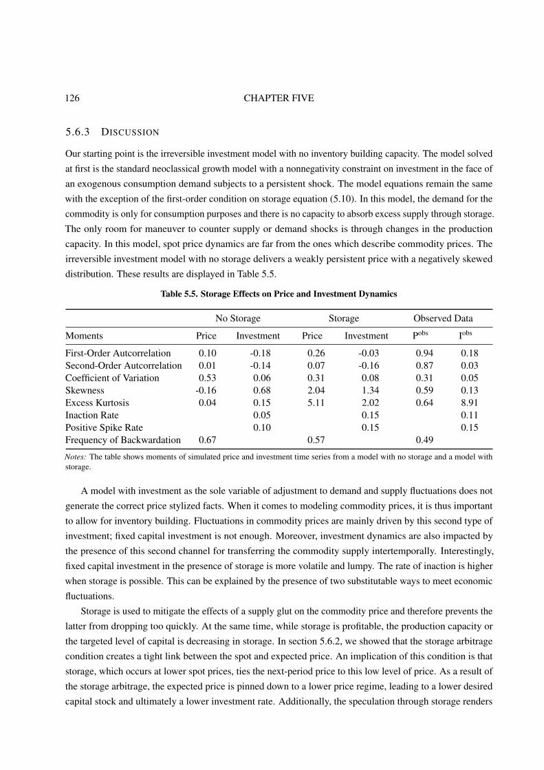
126 CHAPTER FIVE
5.6.3 DISCUSSION
Our starting point is the irreversible investment model with no inventory building capacity. The model solved
at first is the standard neoclassical growth model with a nonnegativity constraint on investment in the face of
an exogenous consumption demand subjects to a persistent shock. The model equations remain the same
with the exception of the first-order condition on storage equation (5.10). In this model, the demand for the
commodity is only for consumption purposes and there is no capacity to absorb excess supply through storage.
The only room for maneuver to counter supply or demand shocks is through changes in the production
capacity. In this model, spot price dynamics are far from the ones which describe commodity prices. The
irreversible investment model with no storage delivers a weakly persistent price with a negatively skewed
distribution. These results are displayed in Table 5.5.
Table 5.5. Storage Effects on Price and Investment Dynamics
No Storage Storage Observed Data
Moments Price Investment Price Investment Pobs Iobs
First-Order Autcorrelation 0.10 -0.18 0.26 -0.03 0.94 0.18Second-Order Autcorrelation 0.01 -0.14 0.07 -0.16 0.87 0.03Coefficient of Variation 0.53 0.06 0.31 0.08 0.31 0.05Skewness -0.16 0.68 2.04 1.34 0.59 0.13Excess Kurtosis 0.04 0.15 5.11 2.02 0.64 8.91Inaction Rate 0.05 0.15 0.11Positive Spike Rate 0.10 0.15 0.15Frequency of Backwardation 0.67 0.57 0.49
Notes: The table shows moments of simulated price and investment time series from a model with no storage and a model withstorage.
A model with investment as the sole variable of adjustment to demand and supply fluctuations does not
generate the correct price stylized facts. When it comes to modeling commodity prices, it is thus important
to allow for inventory building. Fluctuations in commodity prices are mainly driven by this second type of
investment; fixed capital investment is not enough. Moreover, investment dynamics are also impacted by
the presence of this second channel for transferring the commodity supply intertemporally. Interestingly,
fixed capital investment in the presence of storage is more volatile and lumpy. The rate of inaction is higher
when storage is possible. This can be explained by the presence of two substitutable ways to meet economic
fluctuations.
Storage is used to mitigate the effects of a supply glut on the commodity price and therefore prevents the
latter from dropping too quickly. At the same time, while storage is profitable, the production capacity or
the targeted level of capital is decreasing in storage. In section 5.6.2, we showed that the storage arbitrage
condition creates a tight link between the spot and expected price. An implication of this condition is that
storage, which occurs at lower spot prices, ties the next-period price to this low level of price. As a result of
the storage arbitrage, the expected price is pinned down to a lower price regime, leading to a lower desired
capital stock and ultimately a lower investment rate. Additionally, the speculation through storage renders
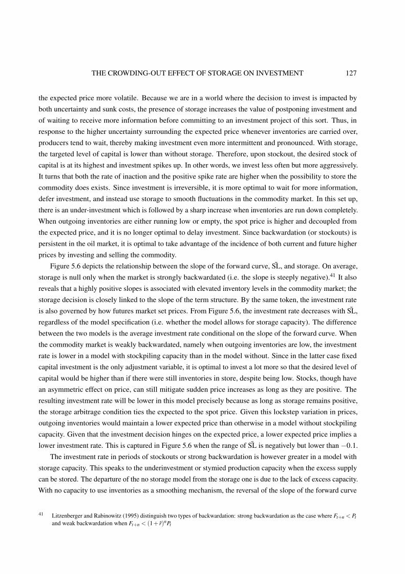
THE CROWDING-OUT EFFECT OF STORAGE ON INVESTMENT 127
the expected price more volatile. Because we are in a world where the decision to invest is impacted by
both uncertainty and sunk costs, the presence of storage increases the value of postponing investment and
of waiting to receive more information before committing to an investment project of this sort. Thus, in
response to the higher uncertainty surrounding the expected price whenever inventories are carried over,
producers tend to wait, thereby making investment even more intermittent and pronounced. With storage,
the targeted level of capital is lower than without storage. Therefore, upon stockout, the desired stock of
capital is at its highest and investment spikes up. In other words, we invest less often but more aggressively.
It turns that both the rate of inaction and the positive spike rate are higher when the possibility to store the
commodity does exists. Since investment is irreversible, it is more optimal to wait for more information,
defer investment, and instead use storage to smooth fluctuations in the commodity market. In this set up,
there is an under-investment which is followed by a sharp increase when inventories are run down completely.
When outgoing inventories are either running low or empty, the spot price is higher and decoupled from
the expected price, and it is no longer optimal to delay investment. Since backwardation (or stockouts) is
persistent in the oil market, it is optimal to take advantage of the incidence of both current and future higher
prices by investing and selling the commodity.
Figure 5.6 depicts the relationship between the slope of the forward curve, S̃L, and storage. On average,
storage is null only when the market is strongly backwardated (i.e. the slope is steeply negative).41 It also
reveals that a highly positive slopes is associated with elevated inventory levels in the commodity market; the
storage decision is closely linked to the slope of the term structure. By the same token, the investment rate
is also governed by how futures market set prices. From Figure 5.6, the investment rate decreases with S̃L,
regardless of the model specification (i.e. whether the model allows for storage capacity). The difference
between the two models is the average investment rate conditional on the slope of the forward curve. When
the commodity market is weakly backwardated, namely when outgoing inventories are low, the investment
rate is lower in a model with stockpiling capacity than in the model without. Since in the latter case fixed
capital investment is the only adjustment variable, it is optimal to invest a lot more so that the desired level of
capital would be higher than if there were still inventories in store, despite being low. Stocks, though have
an asymmetric effect on price, can still mitigate sudden price increases as long as they are positive. The
resulting investment rate will be lower in this model precisely because as long as storage remains positive,
the storage arbitrage condition ties the expected to the spot price. Given this lockstep variation in prices,
outgoing inventories would maintain a lower expected price than otherwise in a model without stockpiling
capacity. Given that the investment decision hinges on the expected price, a lower expected price implies a
lower investment rate. This is captured in Figure 5.6 when the range of S̃L is negatively but lower than −0.1.
The investment rate in periods of stockouts or strong backwardation is however greater in a model with
storage capacity. This speaks to the underinvestment or stymied production capacity when the excess supply
can be stored. The departure of the no storage model from the storage one is due to the lack of excess capacity.
With no capacity to use inventories as a smoothing mechanism, the reversal of the slope of the forward curve
41 Litzenberger and Rabinowitz (1995) distinguish two types of backwardation: strong backwardation as the case where Ft+n < Ptand weak backwardation when Ft+n < (1+ r̃)nPt

128 CHAPTER FIVE
-0.2 -0.1 0 0.1 0.2 0.3 0.4~SL
0
0.05
0.1
0.15
0.2
0.25
Sto
rage
0
0.05
0.1
0.15
0.2
0.25
Inves
tmen
tR
ate
Storage
Investment Rate (with storage)
Investment Rate (without storage)
Figure 5.6. Storage, investment rate and the term structure of futures pricesNotes: The average inventory holdings are calculated for each value of the slope to derive a storage as a function of the shape of theterm structure.
implies an ensuing supply shortage. In a strongly backwardated market (i.e. stockout), the storage arbitrage
no longer holds, which means that the spot price and the expected price are no longer connected to each other.
The difference between the investment rate emanating from the two models, in this case, is related (i) to the
difference in the existing capital stock at the time of stockout and (ii) to the level of uncertainty in a strongly
backwardated market. The first case has already been addressed. It is due to the lower desired capital stocks
when storage can act as a substitute to investments and ends up crowding out investment. The latter point will
be tackled at length in the upcoming discussion. What we can already concluded at this juncture is that, in a
strongly backwardated market, uncertainty in a model with storage capacity is lower than in a model without
it. Finally, when the market is in contango, the difference between the two investment rates is not as stark.
Going one step further in comparing the model with storage capacity and the model without, we look
to the distribution of the slope that each model delivers. We can already see in Figure 5.6, that the range
of S̃L is different between the two models. While the model with storage capacity delivers a more steeply
negatively sloped forward curve than a the model without storage, the latter give a more positively sloped
forward curve. Looking at the distribution of S̃L emerging from the two models, we note that indeed whether
we allow for storage capacity produces two very distinct distributions juxtaposed in Figure 5.7.
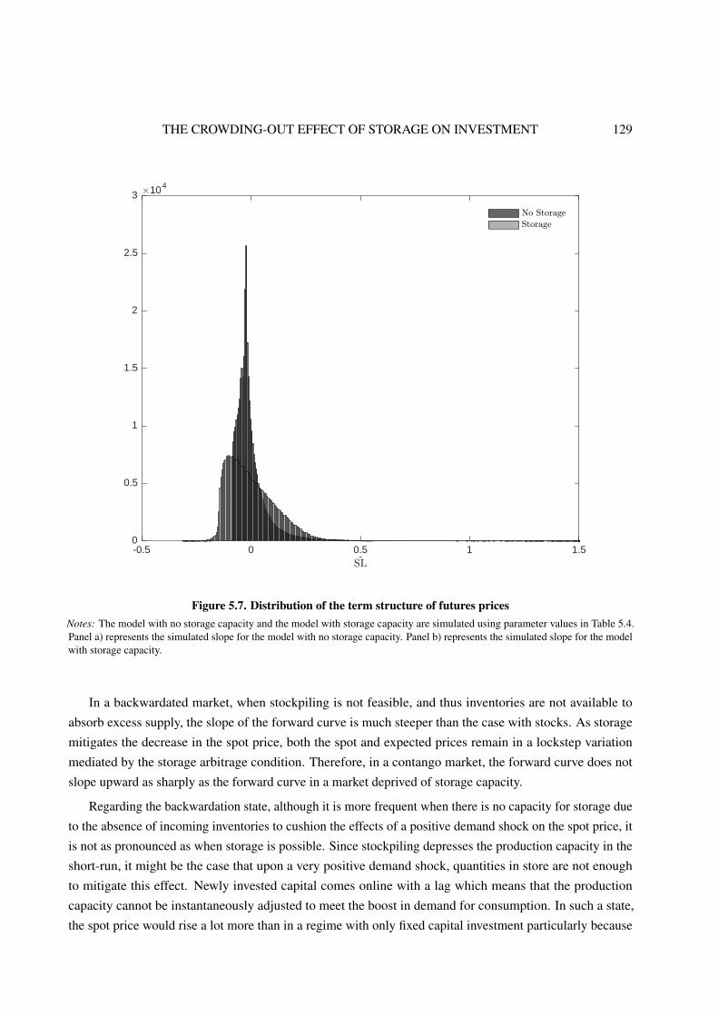
THE CROWDING-OUT EFFECT OF STORAGE ON INVESTMENT 129
-0.5 0 0.5 1 1.5~SL
0
0.5
1
1.5
2
2.5
3 #104
No Storage
Storage
Figure 5.7. Distribution of the term structure of futures pricesNotes: The model with no storage capacity and the model with storage capacity are simulated using parameter values in Table 5.4.Panel a) represents the simulated slope for the model with no storage capacity. Panel b) represents the simulated slope for the modelwith storage capacity.
In a backwardated market, when stockpiling is not feasible, and thus inventories are not available to
absorb excess supply, the slope of the forward curve is much steeper than the case with stocks. As storage
mitigates the decrease in the spot price, both the spot and expected prices remain in a lockstep variation
mediated by the storage arbitrage condition. Therefore, in a contango market, the forward curve does not
slope upward as sharply as the forward curve in a market deprived of storage capacity.
Regarding the backwardation state, although it is more frequent when there is no capacity for storage due
to the absence of incoming inventories to cushion the effects of a positive demand shock on the spot price, it
is not as pronounced as when storage is possible. Since stockpiling depresses the production capacity in the
short-run, it might be the case that upon a very positive demand shock, quantities in store are not enough
to mitigate this effect. Newly invested capital comes online with a lag which means that the production
capacity cannot be instantaneously adjusted to meet the boost in demand for consumption. In such a state,
the spot price would rise a lot more than in a regime with only fixed capital investment particularly because

130 CHAPTER FIVE
storage delays investment. The effect of storage can thus be captured in a higher degree of backwardation
due precisely to the crowding-out effect of storage on investment and the resulting lower production capacity.
As mentioned earlier, the degree of uncertainty is intimately linked to this crowding-out effect. The
storage arbitrage condition, locks both the expected to the spot price thereby transferring the volatility of the
spot price into the future. This very condition results in an increased uncertainty around the expected price.
When uncertainty about the expected price rises, the probability of hitting the lower bound on investment, or
in other words having too much capital, increases as well. As a result, the producer prefers to invest less or
nothing as to avoid being constrained in the future.
While the presence of storage has a strong smoothing effect on the spot price of the commodity, it is
destabilizing for both investment and the expected price. Figure 5.8 illustrates the conditional volatilities
of investment, the spot price and the expected price for both models on the slope of the forward curve.
Introducing storage to an irreversible investment model almost halves the standard deviation of the spot price
(see Table 5.5). The standard deviation of the price is decreasing in the slope of the forward curve when we
-0.2 0 0.2 0.4~SL
0
0.02
0.04
0.06
0.08
0.1
0.12
Sta
ndar
dD
evia
tion
ofI
a) Investment Volatility
-0.2 0 0.2 0.4~SL
0
0.5
1
1.5
2
2.5
Sta
ndar
dD
evia
tion
ofP
b) Spot Price Volatility
-0.2 0 0.2 0.4~SL
0
0.1
0.2
0.3
0.4
0.5
Sta
ndard
Dev
iation
ofF
1
c) 1-month Volatility
With Storage
Without Storage
Figure 5.8. Conditional standard deviation for I, P, and F1
Notes: The standard deviations for I, P, and F1 from the model without storage and the model with storage, are plotted against theslope of the forward curve, S̃L. These moments are computed for each of the 10th percentiles of the distribution of the simulatedtime series {It}T
t=0 and {Pt}Tt=0.
THE CROWDING-OUT EFFECT OF STORAGE ON INVESTMENT 131
allow for storage. Since the latter is positively correlated with storage, the higher is the slope–e.g., the more
inventories there are–the smoother is the spot price. This is not the case for a model without storage. The
conditional volatility of the spot price is V-shaped: it is highest when the market is strongly backwardated,
indicating a supply shortage, dips when the market is moderately satiated so that the forward and spot prices
are closer and spikes again during a supply glut. On the other hand, the volatility of the forward price displays
a V-shape for both models, but the extent to which the volatility changes is different between the two models
depending on the commodity market tightness.
The volatility of the forward price in Figure 5.8 panel c) is directly mirrored in the average investment
rate displayed in Figure 5.6. The investment rate is not only dependent on the expected price but also, given
the nonnegativity constraint, hinges on the degree of future uncertainty. If uncertainty is higher, increasing
the probability of bad spells, the producers will want to avoid being constrained and thus will invest less
today. The presence of storage thus generates higher uncertainty for instances of a weakly backwardated
market. Since in this regime the mass of the slope distribution for the model with storage is the biggest, then
it is often that we are in this region of high uncertainty, which would be accompanied by lower investment
rates. The increased endogenous risk gives way to a more volatile investment rate compared to the stark
irreversible investment model. With storage, investment is always more volatile, except in the case of an
extreme supply glut. A corollary to this result is that the standard deviation of the front-month price rises
more sharply with the slope of the forward curve in a model with no storage capacity. A market in contango,
with no inventory building, generates much more uncertainty for the expected price. This result falls from the
increased smoothness of the spot price that is transferred to the future price through the storage arbitrage
condition. On the other hand, in weak backwardation, the expected price is more volatile when storage is
feasible. In this region of weak backwardation and low outgoing inventories, the forward and spot prices
are still moving together but the spot price volatility is higher. The low excess capacity starts to translate
into higher uncertainty because up until now, the producers have delayed investment more than they would
have if they were not able to store. When outgoing inventories are running low, the spot price becomes more
affected by both disturbances in supply and the persistent demand shock. Since the production capacity
adjusts sluggishly, coupled with low outgoing inventory levels, the expected price will be more volatile than
under the stark model. This excess volatility is the primary reason for which investment is lumpier in a model
with the crowding-out effect of storage. Uncertainty justifies delaying investment since the value of waiting
is higher and dominates the increase in the marginal benefit from investment.
Correspondingly, we can deliver a similar depiction to Figure 5.2 of the relationship between future
uncertainty, investment, and storage for our simulated variables in Figure 5.9. The similarities are really
striking. Indeed, the investment rate is decreasing in inventories, corroborating the relationship between the
investment rate and the slope of the forward curve in Figure 5.6. Furthermore, storage has a destabilizing
effect on the forward price.42 The elevated levels of uncertainty when the amount in store are high explains
also why in this regime the optimal investment rate is lower. As in Figure 5.2, the volatility of the forward
42 The volatility of the subsequent forward prices collapses very rapidly an artifact of this class of models. This is noted inRoutledge et al. (2000) with no clear solution to remedy such a result. For this reason, the subsequent conditional volatility ofthe forward price is not plotted in Figure 5.9.

132 CHAPTER FIVE
20 30 40 50 60 70 80 90 100Storage (%)
0
0.02
0.04
0.06
0.08
0.1
0.12
0.14
0.16
Mea
nIn
vest
men
tR
ate
0.035
0.04
0.045
0.05
0.055
0.06
0.065
0.07
0.075
Futu
rePrice
Vola
tility
(%)
Mean Investment Rate1-month Volatility
Figure 5.9. Conditional volatility of F1 and mean investment rateNotes: The left scale stands for the mean of the simulated investment rate while the right one represents the coefficient of variationof the simulated time series for the front-month price, F1. They both are computed for each 10th percentile of the storage levelsdistribution.
price starts to decrease when the supply glut is at its highest meaning that the storage smoothing effect on the
spot price dominates its destabilizing effect.
All in all, uncertainty about the future, when the producer is constrained and cannot resell his capital
in bad states of the world, makes him more prudent when deciding to invest. This prudence effect of the
nonnegativity constraint on investment is most present when the market is weakly backwardated. The effect
of the irreversibility constraint on investment is strengthened when storage is allowed for. This is a novel
insight and certainly extends our understanding of a firm’s investment decision when it can decide between
two type of investment: fixed capital investment and inventory investment. Additionally, the endogenous risk
that is brought about by the lockstep variation between the spot and the forward price is key in generating the
destabilizing effect of storage on the forward price and the investment rate.
5.7 CONCLUSION
Storage and investment are the two main economic mechanisms serving as the theoretical bedrock of most
of the dynamic commodity models. In addition, the recent development of liquid futures market offers a
THE CROWDING-OUT EFFECT OF STORAGE ON INVESTMENT 133
valuable way to test empirically these forward-looking theories by looking at the market’s reaction to various
shocks and see if they match the model’s predictions. Even from the strict perspective of the operators in
the global market of crude oil, the two most scrutinized metrics are the inventory levels and drilling counts
publicly published on a weekly basis. They are believed to mirror the prevailing supply and demand balance,
where a glut is associated with ballooned inventories and diminishing capital expenditures. This is why we
believe that it is worth to study investment and storage decisions jointly to account for fluctuations in prices,
a point acknowledged but thus far neither explored in the dynamics of capital accumulation nor competitive
storage model literature.
This study aims at filling this gap by building upon three strands of the economics and finance literature
(e.g., capital accumulation, storage and futures pricing) to lay out a partial equilibrium-framework placing
investment and storage at the forefront of the economic decisions dictating the dynamics of a commodity
market. The simulations results obtained on two versions of the model depending whether storage is
acknowledged clearly support the importance of considering both economic mechanisms. They demonstrate
that, at the margin, investment is less profitable whenever storage is possible. Indeed, not only carrying
inventories will weigh on the expected price and in turn the marginal benefit of investing today but also will
raise future uncertainty and thus the options value of waiting and postponing investment. Put another way,
operators invest less often but more aggressively. The deferred investment translate into lower capital stock
and hence a mitigated production capacity. As a result, the commodity becomes scarcer, storing is more
costly, thereby leading to an upward turn in the spot price and a tighter market. The supply and demand
tension is eventually alleviated with a renewed increase in the production capacity through capital investment.
Such a narrative of the cyclical emergence of booms and busts in the oil industry broadly proves to match
the data fairly well. The key insight which emerges out of the confluence of inventory and fixed capital
investment is the implications of lockstep variations in the spot and forward prices on the investment decision.
This tight link between the two prices translates into higher future uncertainty, rendering the nonnegativity
constraint even more penalizing. Ultimately, storage reinforces the irreversibility of investment.
In terms of extensions, it might be worthwhile to study the effects of capital adjustment costs of various
nature–fix, convex and non-convex–in the tradition of Cooper and Haltiwanger (2006) since they are possibly
significant in capital intensive sectors like the oil industry. Among the expected effects of interest are a higher
persistence in production translated into the volatility levels of forward prices which are dying-off too quickly
in our current modeling as compared to the levels observed, although it is a shared drawback among many
dynamic economic models of this kind. Attractive also should be considering the new frictions subsequent to
the introduction of a second but not predetermined factor of production (for e.g., labor known to be the very
first expendable in times of turmoil in the oil market) and the resulting effects on the dynamics implied by the
model. Finally, and perhaps more challenging given the computational issues at stake, it would be to push the
empirical analysis even further in estimating the model key parameters in place of the current calibration.
CHAPTER 6
CONCLUSION
“Essentially, all models are wrong, but some are useful.”
Box and Draper (1987, p.424)
6.1 GENERAL CONCLUSION
In economy as in sciences, a model is an abstraction of the reality, a mathematical representation which
simplifies a phenomenon to be studied and its associated environment so as to reveal the key mechanisms at
stakes, the roles they play and the way they interact with one another. In this regard, the modeling exercise
necessarily requires a set of assumptions to simplify things. This is why, as stated by Box and Draper, to ask
to a model embodying the whole truth, if any, is somewhat utopian and even not really desirable. All that
matters in the end is its usefulness. In economics, a model is useful if it helps to interpret the data, clarify and
organize the thinking, replicate key observed phenomena or else implement conditional forecasts to test and
compare the impacts of alternative policies. The two main metrics to assess the merit of an economic model
are internal and external consistency, the challenge being then to strike the right balance between these two
pillars.
In the context of commodity price volatility studies, looking at the fundamentals of supply, demand
and inventories is a natural place to start thinking about the price behavior in the dynamic and uncertain
world commodity markets. Also natural is to assume that actors in these markets are in competition to
smooth their consumption over time, and thus try their best to predict the future price so as to make their
decisions accordingly. Put in equations, this roughly yields the skeleton of the canonical competitive storage
model along with its associated set of hypotheses. Taking for granted all these theoretical developments
and applying the latest statistical tools available in macroeconometrics, the ultimate objective of the thesis
is to attempt extending the storage model in order to get a more comprehensive understanding of the key
mechanisms governing the booms and busts episodes observed in the global prices of staples goods.
With this in mind, the introducing survey reviews the variety of empirical strategies developed so far
to match the storage theory with the observed data. As is often the case in empirical macroeconomics, the
variety of techniques employed vary in the amount of theoretical constraints imposed on the data. Regardless
CONCLUSION 135
of the ad-hoc or structural approach followed, together the results justify the initial hopes placed in the
storage theory in confirming the empirical relevance of the storage model, thereby strengthening its status as
a promising device to analyze the price variations of basic products on the quantitative front. That said, the
findings also emphasize the numerous pitfalls currently plaguing the storage framework and which, if settled,
could help to answer some of the present puzzling phenomena observed in commodity price series, including
the excessive co-movements and the high levels of serial correlation. Remembering the aforementioned
double criteria of internal and external consistency to deem the performance of a model, the chapter ends
by suggesting a research agenda, gradual in the level of time and effort involved, to improve the model’s
explanatory power and from which originate the three subsequent chapters.
The first contribution is purely empirical. It starts by acknowledging the recent agreement, in the
dedicated literature, about the fact that commodity prices are best described by short to medium-run cyclical
fluctuations around a long-run trend affected by structural breaks. In view of the absence of satisfying
theoretical explanations for these long-term movements a pragmatic empirical strategy has been adopted.
More precisely, the idea, borrowed from the DSGE literature (Canova, 2014), consists in coming up with a
reduced-form representation for the trend which is then jointly estimated with the structural parameters of the
model. With such a statistical repair of the modeling which preserves the internal consistency of the structure,
the model’s deep parameters are found to be more plausible and eventually lowers the level of persistence
in prices to be explained. Put it another way, part of the observed persistence has nothing to do with the
storage theory and, instead, should be explained by the trend. If not it is not only the empirical relevance of
the storage theory but also the reliability of the estimations which might be reduced.
The second contribution is innovative in many respects and I think quite central for the further econometric
work on the storage model, including in the near future. The initial statement is clear: any estimations of
richer specification of the storage model is hampered as long as inference relies on prices information alone,
as has been the case so far. Put differently, reasoning from a price change is too limited an approach for
getting a deeper understanding of the key determinants of the observed dynamics in the commodity markets.
Hence, still inspired from the recent developments in the DSGE literature, we provide an econometric
procedure to take the storage model to the data on both prices and quantities. The latter bring a complement
of information allowing to freely recover additional key parameters among which are the supply elasticity, the
volatility of the production as well as demand structural shocks. Furthermore, as there are more parameters to
estimate, the classical maximum likelihood approach has been replaced with its Bayesian counterparts, more
convenient and widely used to estimate the DSGE model parameters though, as of now, never to infer those
of the storage model. Overall, we believe both these novelties will help paving the way for future research.
Indeed, any serious expansion of the storage model, on both the theoretical and empirical fronts, require
the adoption of a state-space representation of the storage framework as well as the incorporation of data
on quantities in the set of observables, while the Bayesian tools seem more appropriate for recovering the
greater number of parameters.
The last contribution is more theoretical but no less important regarding the future empirical abilities of
the model, at least in the longer-run. Establishing that booms and busts cycles observed in the oil sector are

136 CHAPTER SIX
for the most part a supply and demand story, we think interesting to extend the storage model on the supply
side in accounting for the dynamics of capital accumulation. Intuitively, storage is nothing but another kind
of investment, and thus both should play central roles in driving the spot and future price dynamics in world
commodity markets. This is confirmed by the simulation results obtained with the investment-augmented
storage model which are fairly well supported by the crude oil data. The prime finding is certainly the
crowding-out effect of storage on investment. The main limit of this work is that the model has now three
state variables and thus may be difficult to estimate structurally.
6.2 PERSPECTIVES
Although I hope this dissertation contributed to reinforce the empirical relevance of the competitive storage
model, the latter remains undeniably improvable if, in echo to the introductory citation of Box and Draper
(1987), it is to become an analytical tool “useful” for organizing our thinking about the commodity price
volatility from a quantitative standpoint. In this respect, using a typology similar to the one chosen in
the opening survey, I suggest below some avenues of extensions to be considered at different time scales,
depending on the amount of research energy to be allocated along with the level of computational techniques
required.
NOISY PRICES This is the most natural and straight continuation of the work undertaken in chapter 4.
Indeed, to build upon the latest econometric development of Cafiero et al. (2015) and keep an analytic
form for the Maximum Likelihood estimator, prices have been assumed observed without noises. The latter
assumption is very restrictive in terms of the structural shocks which can be freely identified. Relaxing this
hypothesis will constitute a genuine step toward the evaluation of the fitting performance of more general
specifications of the storage model. Testing alternatives set-ups against one each other will allow for a
comprehensive exploration of the dimensions in which the storage theory does not seem to work well, and
thus indicating in which directions model’s extensions are needed. However, this comes at a computational
cost since, with measurement errors on prices, the likelihood function is no longer tractable and so has to
be simulated using Monte-Carlo approximation techniques. Specifically, the whole estimation procedure
rests on the so-called particle filter, recently introduced in the DSGE literature (Fernández-Villaverde and
Rubio-Ramírez, 2007) but, as far as I know, never applied to the storage model.
MACROECONOMIC FEEDBACKS Alongside the autocorrelation, another puzzle in the commodity price
behavior for which the storage model is unable to account for is the excess of co-movements (Pindyck and
Rotemberg, 1990). As discussed in chapter 2, the integration of macroeconomic spillovers through the interest
rate channel is worth considering for the storage model to be able to capture this kind of richer movements in
and across prices. As is common in empirical macroeconomics, the incorporation of such macroeconomic
forces (e.g., exchanges rates) can be first in the form of an ad-hoc repair deprived of microfoundations,
before ideally being derived from microeconomic principles with the benefit of theoretical advances. On the
CONCLUSION 137
empirical front of this endeavor, the particle filter can well be the powerful tool able to recover, for instance,
the deep parameters of the Frankel (1986)’s overshooting model expressed in a state-space form.
Another benefit of thinking about the interest rate variable as a bridge to connect the storage model with
the complex macroeconomic environment, is its suitability for including the potential effects of the financial
markets. Indeed, the current state of the storage theory and, let alone, the storage model, is almost silent about
the interactions between the physical commodity markets and the financial sector. If the links between the
real economy and finance have long been studied, the Great Recession triggered a race to the financialization
of the macroeconomic models in which the financial industry now plays a key role in driving the business
cycles, and the literature of the storage model can well follow suits. Admittedly, to date the storage model
is a representative-agents based framework with forward-looking and rational expectations. Still, these are
natural and meaningful starting assumptions, not universal rules set in stone.
TWEAKING THE CORE ASSUMPTIONS? It is fair to say that the sharp movements of prices on the world
commodity markets witnessed over the past decade are hardly reconcilable with the fundamentals alone.
With this in mind, dealing with the growing inflow of financial investors likely to trade with sentiments–the
pure “animal spirits”–and thus no real bearing to the fundamentals, and the ultimate consequences on the
commodity prices is at least a natural and fertile field of investigation. This is why, I think there is a place,
in the literature of commodity price volatility, for the effects of financial linkages to explain specific events
such as destabilizing speculative bubbles, episodes of self-fulfilling prophecies, panic and flight to safety,
herding behaviors and other irrational moves alike. From this perspective, one can think in particular about
heterogeneous agents and learning expectations models. Along these lines, of interest is the concept of
rational destabilization developed in De Long et al. (1990) or, close in spirit but more recent, the approach
of Singleton (2014) which consists in introducing informational frictions in the modeling by assuming that
market practitioners have a different interpretation–e.g. “difference of opinions”–about the same publicly
available information related to the economic fundamentals. Conceptually, the traders’ behaviors follow a
learning mechanism in which price expectations are a mix between market fundamentals along with past
and current prices. Together the heterogeneity and learning mechanisms are likely to magnify the up and/or
downward swings in prices similar to the booms and bust cycles. Having said this, it should not be forgotten
that, sooner or later, prices are deemed to revert back to the level dictated by the prevailing physical supply
and demand conditions (Knittel and Pindyck, 2016). As a result, the financial economics literature is torn
apart about the real influence speculation actually has on the prices of primary products, driving them away
from the market fundamentals. The thing is that the publicly available data is sparse, of poor reliability and
so not very insightful for attempting to fix the controversy in quantitative terms. Add to this data problem,
both the numerous methodological and computational challenges involved, and there are all the ingredients
for making the introduction of finance into the storage theory a very long-winded undertaking.
NO BLACK BOXES As a last remark, to keep working with parsimonious models with crystal clear inner-
workings, I do not think reasonable to try adding all these potential extensions in a single framework with
the vain hope of matching the whole diversity of patterns observed in the data. More realistic would be to

138 CHAPTER SIX
build and structurally estimate different versions of the storage model, incorporating one or a few of the
aforementioned developments, and for eventually being able to deliver reliable answers to questions posed
conditional on a given set of circumstances (e.g., normal times vs markets turmoil).
In sum, in spite of all what has already been achieved to rekindle the interest and usefulness of the
competitive storage model, there are still many precious insights which are yet to be learned from this tool.
For all these reasons future work in this area are part of a very exciting and dynamic research program.
Bibliography
Abel, A. B. and Eberly, J. C. (1994). A unified model of investment under uncertainty. The AmericanEconomic Review, 84(5), 1369–1384.
Adjemian, M. K. and Smith, A. (2012). Using USDA forecasts to estimate the price flexibility of demand foragricultural commodities. American Journal of Agricultural Economics, 94(4), 978–995.
Adrangi, B. and Chatrath, A. (2003). Non-linear dynamics in futures prices: evidence from the coffee, sugarand cocoa exchange. Applied Financial Economics, 13(4), 245–256.
Alhajji, A. and Huettner, D. (2000). OPEC and other commodity cartels: a comparison. Energy Policy,28(15), 1151 – 1164.
Arezki, R., Hadri, K., Loungani, P. and Rao, Y. (2014). Testing the Prebisch-Singer hypothesis since 1650:Evidence from panel techniques that allow for multiple breaks. Journal of International Money andFinance, 42, 208–223.
Bachmann, R., Caballero, R. J. and Engel, E. M. R. A. (2013). Aggregate implications of lumpy investment:New evidence and a DSGE model. American Economic Journal: Macroeconomics, 5(4), 29–67.
Bachmann, R. and Ma, L. (2016). Lumpy investment, lumpy inventories. Journal of Money, Credit andBanking, 48(5), 821–855.
Balagtas, J. V. and Holt, M. T. (2009). The commodity terms of trade, unit roots, and nonlinear alternatives:A smooth transition approach. American Journal of Agricultural Economics, 91(1), 87–105.
Barnett, W. A., Gallant, A. R., Hinich, M. J., Jungeilges, J. A., Kaplan, D. T. and Jensen, M. J. (1995).Robustness of nonlinearity and chaos tests to measurement error, inference method, and sample size.Journal of Economic Behavior & Organization, 27(2), 301–320.
Barnett, W. A., He, Y. et al. (2001). Unsolved econometric problems in nonlinearity, chaos, and bifurcation.Central European Journal of Operations Research, 9, 147–182.
Barro, R. J. and Sala-i Martin, X. (1990). World real interest rates. In O. J. Blanchard and S. Fischer (eds.)NBER Macroeconomics Annual 1990, volume 5, chapter 1, (pp. 15–74). Cambridge, MA: MIT Press.
Basak, S. and Pavlova, A. (2016). A model of financialization of commodities. The Journal of Finance, 71(4),1511–1556.
Baumeister, C. and Hamilton, J. D. (2015). Structural Interpretation of Vector Autoregressions with Incom-plete Identification: Revisiting the Role of Oil Supply and Demand Shocks. Technical report.
Baumeister, C. and Kilian, L. (2016). Forty years of oil price fluctuations: Why the price of oil may stillsurprise us. Journal of Economic Perspectives, 30(1), 139–60.
Beck, S. (2001). Autoregressive conditional heteroscedasticity in commodity spot prices. Journal of AppliedEconometrics, 16(2), 115–132.
Bertola, G. and Caballero, R. J. (1994). Irreversibility and aggregate investment. The Review of EconomicStudies, 61(2), 223–246.
140 BIBLIOGRAPHY
Bobenrieth, E. S. A., Bobenrieth, J. R. A., Wright, B. D. and Zeng, D. (2014). How Biofuels PoliciesBoosted Grain Staple Prices: A Counterfactual Analysis. Paper 5125, Agricultural and Applied EconomicsAssociation, 2014 Annual Meeting, July 27–29, 2014, Minneapolis, Minnesota.
Bobenrieth, E. S. A., Wright, B. D. and Zeng, D. (2013). Stocks-to-use ratios as indicators of vulnerability tospikes in global cereal markets. Agricultural Economics, 44(S1), 43–52.
Bordo, M. D. (1980). The effects of monetary change on relative commodity prices and the role of long-termcontracts. Journal of Political Economy, 88(6), 1088–1109.
Box, G. E. and Draper, N. R. (1987). Empirical model-building and response surfaces. Wiley New York.Brennan, M. J. (1958). The supply of storage. The American Economic Review, 48(1), 50–72.Brennan, M. J. and Schwartz, E. S. (1985). Evaluating natural resource investments. The Journal of Business,
58(2), 135–157.Brock, W. A. and Hommes, C. H. (1997). A rational route to randomness. Econometrica, 65(5), 1059–1095.Browne, F. and Cronin, D. (2010). Commodity prices, money and inflation. Journal of Economics and
Business, 62(4), 331–345.Buchanan, N. S. (1939). A reconsideration of the cobweb theorem. Journal of Political Economy, 47(1),
67–81.Caballero, R. J. (1999). Aggregate investment. volume 1, Part B of Handbook of Macroeconomics, chapter 12,
(pp. 813 – 862). Elsevier.Caballero, R. J. and Engel, E. M. R. A. (1999). Explaining investment dynamics in U.S. manufacturing: A
generalized (S, s) approach. Econometrica, 67(4), 783–826.Cafiero, C., Bobenrieth, E. S. A. and Bobenrieth, J. R. A. (2011a). Storage arbitrage and commodity price
volatility. In A. Prakash (ed.) Safeguarding food security in volatile global markets, chapter 15, (pp.288–313). Rome: FAO.
Cafiero, C., Bobenrieth, E. S. A., Bobenrieth, J. R. A. and Wright, B. D. (2011b). The empirical relevance ofthe competitive storage model. Journal of Econometrics, 162(1), 44–54.
Cafiero, C., Bobenrieth, E. S. A., Bobenrieth, J. R. A. and Wright, B. D. (2015). Maximum Likelihoodestimation of the standard commodity storage model: Evidence from sugar prices. American Journal ofAgricultural Economics, 97(1), 122–136.
Cafiero, C. and Wright, B. D. (2006). Is the storage model a ’closed’ empirical issue? The empirical abilityof the storage model to explain price dynamics. In A. Sarris and D. Hallam (eds.) Agricultural CommodityMarkets and Trade. New Approaches to Analyzing Market Structure and Instability, chapter 4, (pp. 89–114).Northampton: FAO/Edward Elgar.
Canova, F. (1998). Detrending and business cycle facts: A user’s guide. Journal of Monetary Economics,41(3), 533–540.
Canova, F. (2014). Bridging DSGE models and the raw data. Journal of Monetary Economics, 67, 1–15.Carlson, M., Khokher, Z. and Titman, S. (2007). Equilibrium exhaustible resource price dynamics. The
Journal of Finance, 62(4), 1663–1703.Carroll, C. D. (2006). The method of endogenous gridpoints for solving dynamic stochastic optimization
problems. Economics Letters, 91(3), 312–320.Cashin, P. and McDermott, C. J. (2002). The long-run behavior of commodity prices: Small trends and big
variability. IMF Staff Papers, 49(2), 175–199.Chambers, M. J. and Bailey, R. E. (1996). A theory of commodity price fluctuations. Journal of Political
BIBLIOGRAPHY 141
Economy, 104(5), 924–957.Chambers, R. G. and Just, R. E. (1979). A critique of exchange rate treatment in agricultural trade models.
American Journal of Agricultural Economics, 61(2), 249–257.Chambers, R. G. and Just, R. E. (1982). An investigation of the effect of monetary factors on agriculture.
Journal of Monetary Economics, 9(2), 235–247.Chatrath, A., Adrangi, B. and Dhanda, K. K. (2002). Are commodity prices chaotic? Agricultural Economics,
27(2), 123–137.Chen, Y.-C., Rogoff, K. S. and Rossi, B. (2010). Can exchange rates forecast commodity prices? The
Quarterly Journal of Economics, 125(3), 1145–1194.Ching-chong, L., Shih-wen, H. and Chih-ping, F. (2005). The overshooting hypothesis of agricultural prices:
The role of asset substitutability. Journal of Agricultural and Resource Economics, 30(1), 128–150.Cooper, J. C. (2003). Price elasticity of demand for crude oil: estimates for 23 countries. OPEC Review,
27(1), 1–8.Cooper, R. W. and Haltiwanger, J. C. (2006). On the nature of capital adjustment costs. The Review of
Economic Studies, 73(3), 611–633.Cootner, P. H. (1960). Returns to speculators: Telser versus Keynes. Journal of Political Economy, 68(4),
396–404.Cuddington, J. T. and Nülle, G. (2014). Variable long-term trends in mineral prices: The ongoing tug-of-war
between exploration, depletion, and technological change. Journal of International Money and Finance,42, 224–252.
Dahl, C. (1993). A survey of oil demand elasticities for developing countries. OPEC Review, 17(4), 399–420.Darrell Duffie, K. J. S. (1993). Simulated moments estimation of markov models of asset prices. Econometrica,
61(4), 929–952.De Long, J. B., Shleifer, A., Summers, L. H. and Waldmann, R. J. (1990). Positive feedback investment
strategies and destabilizing rational speculation. The Journal of Finance, 45(2), 379–395.Deaton, A. (1999). Commodity prices and growth in Africa. The Journal of Economic Perspectives, 13(3),
23–40.Deaton, A. and Laroque, G. (1992). On the behaviour of commodity prices. Review of Economic Studies,
59(1), 1–23.Deaton, A. and Laroque, G. (1995). Estimating a nonlinear rational expectations commodity price model
with unobservable state variables. Journal of Applied Econometrics, 10, S9–S40.Deaton, A. and Laroque, G. (1996). Competitive storage and commodity price dynamics. Journal of Political
Economy, 104(5), 896–923.Dewally, M., Ederington, L. H. and Fernando, C. S. (2013). Determinants of trader profits in commodity
futures markets. Review of Financial Studies, 26(10), 2648–2683.Dixit, A. (1992). Investment and hysteresis. Journal of Economic Perspectives, 6(1), 107–132.Dixit, A. K. and Pindyck, R. S. (1994). Investment under uncertainty. Princeton University Press.Doms, M. and Dunne, T. (1998). Capital adjustment patterns in manufacturing plants. Review of Economic
Dynamics, 1(2), 409–429.Dornbusch, R. (1976). Expectations and exchange rate dynamics. Journal of Political Economy, 84(6),
1161–76.Dvir, E. and Rogoff, K. (2009). The Three Epochs of Oil. Boston College Working Papers in Economics 706,
142 BIBLIOGRAPHY
Boston College Department of Economics.Dvir, E. and Rogoff, K. S. (2014). Demand effects and speculation in oil markets: Theory and evidence.
Journal of International Money and Finance, 42, 113–128.Engel, C. and West, K. (2005). Exchange rates and fundamentals. Journal of Political Economy, 113(3),
485–517.Ezekiel, M. (1938). The cobweb theorem. The Quarterly Journal of Economics, 52(2), 255–280.Fama, E. F. and French, K. R. (1988). Business cycles and the behavior of metals prices. The Journal of
Finance, 43(5), 1075–1093.Fernández-Villaverde, J. (2010). The econometrics of DSGE models. SERIEs, 1(1–2), 3–49.Fernández-Villaverde, J., Rubio-Ramírez, J. F. and Schorfheide, F. (forthcoming). Solution and estimation
methods for DSGE models. In J. Taylor and H. Uhlig (eds.) Handbook of Macroeconomics, volume 2.Amsterdam: Elsevier.
Fernández-Villaverde, J. and Rubio-Ramírez, J. F. (2007). Estimating macroeconomic models: A likelihoodapproach. The Review of Economic Studies, 74(4), 1059–1087.
Ferroni, F. (2011). Trend agnostic one-step estimation of DSGE models. The B.E. Journal of Macroeconomics,11(1), 1–36.
Frankel, J. A. (1986). Expectations and commodity price dynamics: The overshooting model. AmericanJournal of Agricultural Economics, 68(2), 344–348.
Frankel, J. A. (2014). Effects of speculation and interest rates in a "carry trade" model of commodity prices.Journal of International Money and Finance, 42, 88–112.
Frankel, J. A. and Hardouvelis, G. A. (1985). Commodity prices, money surprises and fed credibilit. Journalof Money, Credit and Banking, 17(4), 425–438.
Gallant, A. and Tauchen, G. (1996). Which moments to match? Econometric Theory, 12(04), 657–681.Geweke, J. (1992). Evaluating the accuracy of sampling-based approaches to the calculation of posterior
moments. In J. M. Bernardo, J. O. Berger, A. P. Dawid and A. F. M. Smith (eds.) Bayesian Statistics4: Proceedings of the Fourth Valencia International Meeting, New York: Oxford University Press, (pp.169–193).
Ghoshray, A. (2011). A reexamination of trends in primary commodity prices. Journal of DevelopmentEconomics, 95(2), 242–251.
Gilbert, C. L. (1987). International commodity agreements: Design and performance. World Development,15(5), 591–616.
Gilbert, C. L. (1989). The impact of exchange rates and developing country debt on commodity prices.Economic Journal, 99(397), 773–784.
Gilbert, C. L. (1995). Modelling market fundamentals: A model of the aluminium market. Journal of AppliedEconometrics, 10(4), 385–410.
Gilbert, C. L. (1996). International commodity agreements: An obituary notice. World Development, 24(1),1–19.
de Gorter, H., Drabik, D. and Just, D. R. (2015). The Economics of Biofuel Policies: Impacts on PriceVolatility in Grain and Oilseed Markets. New York: Palgrave macmillan.
Gorton, G. B., Hayashi, F. and Rouwenhorst, K. G. (2012). The fundamentals of commodity futures returns.Review of Finance, 17(1), 35–105.
Gouel, C. (2012). Agricultural price instability: A survey of competing explanations and remedies. Journal

BIBLIOGRAPHY 143
of Economic Surveys, 26(1), 129–156.Gouel, C. (2013a). Comparing numerical methods for solving the competitive storage model. Computational
Economics, 41(2), 267–295.Gouel, C. (2013b). RECS: MATLAB Solver for Rational Expectations Models with Complementarity
Equations - Version 0.6, available at www.recs-solver.org.Gouel, C. and Legrand, N. (2016a). Bayesian Estimation of the Storage Model using Information on
Quantities. Technical report, Agricultural and Applied Economics Association, 2016 Annual Meeting, July31-August 2, 2016, Boston, Massachusetts.
Gouel, C. and Legrand, N. (2016b). Estimating the competitive storage model with trending commodityprices. Journal of Applied Econometrics, forthcoming.
Gourieroux, C., Monfort, A. and Renault, E. (1993). Indirect inference. Journal of Applied Econometrics,8(S1), S85–S118.
Gourieroux, C., Monfort, A. and Trognon, A. (1984). Pseudo maximum likelihood methods: Theory.Econometrica, 52(3), 681–700.
Grilli, E. R. and Yang, M. C. (1988). Primary commodity prices, manufactured goods prices, and the termsof trade of developing countries: What the long run shows. World Bank Economic Review, 2(1), 1–47.
Guerra, E. A., Bobenrieth H., E. S. A., Bobenrieth H., J. R. A. and Cafiero, C. (2015). Empirical commoditystorage model: the challenge of matching data and theory. European Review of Agricultural Economics,42(4), 607–623.
Gustafson, R. L. (1958). Carryover Levels for Grains: A Method for Determining Amounts that are OptimalUnder Specified Conditions. Technical Bulletin 1178, US Dept. of Agriculture.
Hamilton, J. D. (1994). Time Series Analysis. Princeton: Princeton University Press.Hamilton, J. D. (2009). Understanding crude oil prices. The Energy Journal, 30(2), 179–206.Hansen, L. P. and Singleton, K. J. (1982). Generalized instrumental variables estimation of nonlinear rational
expectations models. Econometrica, 50(5), 1269–1286.Harrell, F. E. (2001). Regression Modeling Strategies: With Applications to Linear Models, Logistic
Regression, and Survival Analysis. New York: Springer.Harvey, A. C. and Jaeger, A. (1993). Detrending, stylized facts and the business cycle. Journal of Applied
Econometrics, 8(3), 231–247.Harvey, D. I., Kellard, N. M., Madsen, J. B. and Wohar, M. E. (2010). The Prebisch-Singer hypothesis: Four
centuries of evidence. The Review of Economics and Statistics, 92(2), 367–377.Inoue, A. and Kilian, L. (2013). Inference on impulse response functions in structural VAR models. Journal
of Econometrics, 177(1), 1 – 13.International Monetary Fund (2014). World Economic Outlook: Recovery strengthens, Remains uneven.
Washington, DC: International Monetary Fund.Jabara, C. L. and Schwartz, N. E. (1987). Flexible exchange rates and commodity price changes: The case of
Japan. American Journal of Agricultural Economics, 69(3), 580–590.Jacks, D. S., O’Rourke, K. H. and Williamson, J. G. (2011). Commodity price volatility and world market
integration since 1700. Review of Economics and Statistics, 93(3), 800–813.Johansen, S. (1988). Statistical analysis of cointegration vectors. Journal of Economic Dynamics and Control,
12(2), 231–254.Kaldor, N. (1939). Speculation and economic stability. The Review of Economic Studies, 7(1), 1–27.
144 BIBLIOGRAPHY
Kaminsky, G. L., Reinhart, C. M. and Végh, C. A. (2003). The unholy trinity of financial contagion. Journalof Economic Perspectives, 17(4), 51–74.
Kellard, N. M. and Wohar, M. E. (2006). On the prevalence of trends in primary commodity prices. Journalof Development Economics, 79(1), 146–167.
Kellogg, R. (2014). The effect of uncertainty on investment: Evidence from texas oil drilling. AmericanEconomic Review, 104(6), 1698–1734.
Kilian, L. (2008). Exogenous oil supply shocks: How big are they and how much do they matter for the u.s.economy? The Review of Economics and Statistics, 90(2), 216–240.
Kilian, L. (2009). Not all oil price shocks are alike: Disentangling demand and supply shocks in the crude oilmarket. The American Economic Review, 99(3), 1053–1069.
Kilian, L. and Murphy, D. P. (2014). The role of inventories and speculative trading in the global market forcrude oil. Journal of Applied Econometrics, 29(3), 454–478.
Knittel, C. R. and Pindyck, R. S. (2016). The simple economics of commodity price speculation. AmericanEconomic Journal: Macroeconomics, 8(2), 85–110.
Kogan, L., Livdan, D. and Yaron, A. (2009). Oil futures prices in a production economy with investmentconstraints. The Journal of Finance, 64(3), 1345–1375.
Krautkraemer, J. A. (1998). Nonrenewable resource scarcity. Journal of Economic Literature, 36(4), 2065–2107.
Kung, H. and Schmid, L. (2015). Innovation, growth, and asset prices. The Journal of Finance, 70(3),1001–1037.
Labys, W. C. (1973). Dynamic Commodity Models: Specification, Estimation and Simulation. Lexington,MA:Lexington Books.
Labys, W. C. (2006). Modeling and forecasting primary commodity prices. Ashgate Publishing, Ltd.Lee, J. and Strazicich, M. C. (2003). Minimum Lagrange multiplier unit root test with two structural breaks.
The Review of Economics and Statistics, 85(4), 1082–1089.Litzenberger, R. H. and Rabinowitz, N. (1995). Backwardation in oil futures markets: Theory and empirical
evidence. The Journal of Finance, 50(5), 1517–1545.Lowry, M., Glauber, J., Miranda, M. and Helmberger, P. (1987). Pricing and storage of field crops: A
quarterly model applied to soybeans. American Journal of Agricultural Economics, 69(4), 740–749.Lucas, J., Robert. E. (1976). The Phillips curve and labor markets. volume 1 of Carnegie-Rochester
conference series on public policy, (pp. 19–46). Elsevier.Michaelides, A. and Ng, S. (2000). Estimating the rational expectations model of speculative storage: A
Monte Carlo comparison of three simulation estimators. Journal of Econometrics, 96(2), 231–266.Miranda, M. J. and Rui, X. (1999). An empirical reassessment of the commodity storage model, mimeo, The
Ohio State University.Muth, J. F. (1961). Rational expectations and the theory of price movements. Econometrica, 29(3), 315–335.Nerlove, M. and Bessler, D. A. (2001). Chapter 3 expectations, information and dynamics. In B. L. Gardner
and G. C. Rausser (eds.) Agricultural Production, volume 1, Part A of Handbook of Agricultural Economics,(pp. 155 – 206). Elsevier.
Ng, S. (1996). Looking for evidence of speculative stockholding in commodity markets. Journal of EconomicDynamics and Control, 20(1-3), 123–143.
Ng, S. and Ruge-Murcia, F. J. (2000). Explaining the persistence of commodity prices. Computational
BIBLIOGRAPHY 145
Economics, 16, 149–171.Ng, V. K. and Pirrong, S. C. (1994). Fundamentals and volatility: Storage, spreads, and the dynamics of
metals prices. The Journal of Business, 67(2), 203–230.Nocedal, J. and Wright, S. J. (2006). Numerical Optimization. New York: Springer.Osborne, T. (2004). Market news in commodity price theory: Application to the Ethiopian grain market. The
Review of Economic Studies, 71(1), 133–164.Pavlova, A. and Rigobon, R. (2007). Asset prices and exchange rates. The Review of Financial Studies, 20(4),
1139–1181.Pfaffenzeller, S., Newbold, P. and Rayner, A. (2007). A short note on updating the Grilli and Yang commodity
price index. World Bank Economic Review, 21(1), 151–163.Pindyck, R. S. (1991). Irreversibility, uncertainty, and investment. Journal of Economic Litterature, 29(3),
1110–1148.Pindyck, R. S. and Rotemberg, J. J. (1990). The excess co-movement of commodity prices. The Economic
Journal, 100(403), 1173–1189.Pindyck, R. S. and Rotemberg, J. J. (1993). The comovement of stock prices. The Quarterly Journal of
Economics, 108(4), 1073–1104.Prebisch, R. (1950). The economic development of Latin America and its principal problems. New York:
United Nations.Prescott, E. C. (1977). Should control theory be used for economic stabilization? Carnegie-Rochester
Conference Series on Public Policy, 7, 13–38.Ridler, D. and Yandle, C. A. (1972). A simplified method for analyzing the effects of exchange rate changes
on exports of a primary commodity. Staff Papers - International Monetary Fund, 19(3), 559–578.Rios, L. M. and Sahinidis, N. V. (2013). Derivative-free optimization: a review of algorithms and comparison
of software implementations. Journal of Global Optimization, 56(4), 1247–1293.Robert, C. and Casella, G. (2004). Monte Carlo Statistical Methods. New York: Springer-Verlag.Roberts, M. J. and Schlenker, W. (2013). Identifying supply and demand elasticities of agricultural commodi-
ties: Implications for the US ethanol mandate. The American Economic Review, 103(6), 2265–2295.Rossi, B. (2005). Optimal tests for nested model selection with underlying parameter insatbility. Econometric
Theory, 21, 962–990.Routledge, B. R., Seppi, D. J. and Spatt, C. S. (2000). Equilibrium forward curves for commodities. The
Journal of Finance, 55(3), 1297–1338.Saghaian, S. H., Hasan, M. F. and Reed, M. R. (2002). Overshooting of agricultural prices in four asian
economies. Journal of Agricultural and Applied Economics, 34(01), 95–109.Sargent, T. J. (1976). A classical macroeconometric model for the united states. Journal of Political Economy,
84(2), 207–237.Schuh, G. E. (1974). The exchange rate and U. S. agriculture. American Journal of Agricultural Economics,
56(1), 1–13.Schwartz, E. S. (1997). The stochastic behavior of commodity prices: Implications for valuation and hedging.
The Journal of Finance, 52(3), 923–973.Schwartz, E. S. and Smith, J. E. (2000). Short-term variations and long-term dynamics in commodity prices.
Management Science, 46(7), 893–911.Seale, J. L., Jr. and Regmi, A. (2006). Modeling international consumption patterns. Review of Income and
146 BIBLIOGRAPHY
Wealth, 52(4), 603–624.Sims, C. A. (1980). Macroeconomics and reality. Econometrica, 48(1), 1–48.Singer, H. W. (1950). The distribution of gains between investing and borrowing countries. The American
Economic Review, 40(2), 473–485.Singleton, K. J. (2014). Investor flows and the 2008 boom/bust in oil prices. Management Science, 60(2),
300–318.Smets, F. and Wouters, R. (2007). Shocks and frictions in us business cycles: A bayesian dsge approach. The
American Economic Review, 97(3), 586–606.Smith, J. (2005). Inscrutable OPEC? Behavioral tests of the cartel hypothesis. The Energy Journal, Volume
26(1), 51–82.Telser, L. G. (1958). Futures trading and the storage of cotton and wheat. Journal of Political Economy,
66(3), 233–255.Thomas, J. K. (2002). Is lumpy investment relevant for the business cycle? Journal of Political Economy,
110, 508–534.Tong, H. and Lim, K. S. (1980). Threshold autoregression, limit cycles and cyclical data. Journal of the
Royal Statistical Society. Series B, 42, 245–292.Varian, H. R. (1989). What use is economic theory? Technical report.Vaz, A. I. F. and Vicente, L. N. (2007). A particle swarm pattern search method for bound constrained global
optimization. Journal of Global Optimization, 39(2), 197–219.Veldkamp, L. L. (2006). Information markets and the comovement of asset prices. The Review of Economic
Studies, 73(3), 823–845.Vihola, M. (2012). Robust adaptive Metropolis algorithm with coerced acceptance rate. Statistics and
Computing, 22(5), 997–1008.Westerhoff, F. and Reitz, S. (2005). Commodity price dynamics and the nonlinear market impact of technical
traders: empirical evidence for the {US} corn market. Physica A: Statistical Mechanics and its Applications,349(3-4), 641–648.
Williams, J. C. and Wright, B. D. (1991). Storage and commodity markets. Cambridge University Press.Williamson, L. and Williamson, P. (1942). What we eat. Journal of Farm Economics, 24(3), 698–703.Working, H. (1949). The theory of price of storage. The American Economic Review, 39(6), 1254–1262.World Bank and FAO (2012). The Grain Chain: Food Security and Managing Wheat Imports in Arab
Countries. Washington, DC: World Bank.Wright, B. D. (2014). Global biofuels: Key to the puzzle of grain market behavior. Journal of Economic
Perspectives, 28(1), 73–98.Wright, B. D. and Williams, J. C. (1982). The economic role of commodity storage. The Economic Journal,
92(367), 596–614.Wright, B. D. and Williams, J. C. (1984). The welfare effects of the introduction of storage. The Quarterly
Journal of Economics, 99(1), 169–192.Yamada, H. and Yoon, G. (2014). When Grilli and Yang meet Prebisch and Singer: Piecewise linear trends
in primary commodity prices. Journal of International Money and Finance, 42, 193–207.Zeng, D. (2012). Out of sight, out of mind? Estimating commodity price dynamics using detrended price,
mimeo, UC Berkeley.