Threshold Effects in Multivariate Error Correction Models∗

Jesus Gonzalo

Universidad Carlos III de Madrid

Jean-Yves Pitarakis

University of Southampton

Abstract

In this paper we propose a testing procedure for assessing the presence of threshold effects

in nonstationary Vector autoregressive models with or without cointegration. Our approach

involves first testing whether the long run impact matrix characterising the VECM type rep-

resentation of the VAR switches according to the magnitude of some threshold variable and

is valid regardless of whether the system is purely I(1), I(1) with cointegration or stationary.

Once the potential presence of threshold effects is established we subsequently evaluate the

cointegrating properties of the system in each regime through a model selection based approach

whose asymptotic and finite sample properties are also established. This subsequently allows us

to introduce a novel non-linear permanent and transitory decomposition of the vector process

of interest.

∗We wish to thank the Spanish Ministry of Education for supporting this research under grant SEJ2004-0401ECON

1 Introduction

A growing body of research in the recent time series literature has concentrated on incorporating

nonlinear behaviour in conventional linear reduced form specifications such as autoregressive and

moving average models. The motivation for moving away from the traditional linear model with

constant parameters has typically come from the observation that many economic and financial time

series are often characterised by regime specific behaviour and asymmetric responses to shocks. For

such series the linearity and parameter constancy restrictions are typically inappropriate and may

lead to misleading inferences about their dynamics.

Within this context, and a univariate setting, a general class of models that has been particularly

popular from both a theoretical and applied perspective is the family of threshold models which

are characterised by piecewise linear processes separated according to the magnitude of a threshold

variable which triggers the changes in regime. When each linear regime follows an autoregressive

process for instance we have the well known threshold autoregressive class of models, the statistical

properties of which have been investigated in the early work of Tong and Lim (1980), Tong (1983,

1990), Tsay (1989), Chan (1990, 1993) and more recently reconsidered and extended in Hansen

(1996, 1997, 1999a, 1999b, 2000), Caner and Hansen (2001), Gonzalez and Gonzalo (1997), Gonzalo

and Montesinos (2000), Gonzalo and Pitarakis (2002) among others. The two key aspects on which

this theoretical research has focused on were the development of a distributional theory for tests

designed to detect the presence of threshold effects and the statistical properties of the resulting

parameter estimators characterising such models.

Given their ability to capture a very rich set of dynamic behaviour including persistence and

asymmetries, the use of this class of models has been advocated in numerous applications aiming

to capture economically meaningful nonlinearities. Examples include the analysis of asymmetries

in persistence in the US output growth (Beaudry and Koop (1993), Potter (1995)), asymmetries in

the response of output prices to input price increases versus decreases (Borenstein, Cameron and

Gilbert (1997), Peltzman (2000)), nonlinearities in unemployment rates (Hansen (1997), Koop and

Potter (1999)), threshold effects in cross-country growth regressions (Durlauf and Johnson (1995))

and in international relative prices (Michael, Nobay and Peel (1997), Obstfeld and Taylor (1997),

O’Connell and Wei (1997), Lo and Zivot (2001)) among numerous others.

1

Although the vast majority of the theoretical developments in the area of testing and estima-

tion of univariate threshold models have been obtained under the assumption of stationarity and

ergodicity, another important motivation for their popularity came from the observation that a

better description of the dynamics of numerous economic variables can be achieved by interacting

the pervasive nature of unit roots with that of threshold effects within the same specification. This

was also motivated by the observation that there might be much weaker support for the unit root

hypothesis when the alternative hypothesis under consideration allows for the presence of thresh-

old type effects in the time series of interest. In Pippenger and Goering (1993) for instance the

authors documented a substantial fall in the power of the Dickey Fuller test when the stationary

alternative was allowed to include threshold effects. This also motivated the work of Enders and

Granger (1998), who proposed a simple test of the null hypothesis of a unit root against asymmetric

adjustment instead of a linear stationary alternative.

One important property of threshold models that contributed to this line of research is their

ability to capture persistent behaviour while remaining globally stationary. This can be achieved

for instance by allowing a time series to follow a unit root type process such as a random walk

within one regime while being stationary in another. Numerous economic and financial variables

such as unemployment rates or interest rates for instance must be stationary by the mere fact that

they are bounded. However at the same time conventional unit roots tests are typically unable to

reject the null hypothesis of a unit root in their autoregressive representation. This observation has

prompted numerous researchers to explore the possibility that the dynamics of these series may be

better described by threshold models that allow the nonstationary component to occur within a

corridor regime. A well known example highlighting this point is the behaviour of real exchange

rate series which are typically found to be unit root processes, implying lack of international arbi-

trage and violation of the PPP hypothesis. Once allowance is made for the presence of threshold

effects capturing aspects such as transaction costs however it has been typically found that this

nonstationarity only occurs locally (e.g. between transaction cost bounds) and that the process is in

fact globally stationary (see Bec, Ben-Salem and Carrasco (2001) and references therein). Within a

related context, Gonzalez and Gonzalo (1998) also introduced a globally stationary process referred

to as a threshold unit root model that combines the presence of a unit root with threshold effects,

and found strong support in favour of such a specification for modelling interest rate series.

Although all of the above mentioned research operated under a univariate setup the recent

2

time series literature has also witnessed a growing interest in the inclusion of threshold effects in

multivariate settings such as vector error correction models. A key factor that triggered this line

of research has been the observation that threshold effects may also have an intuitive appeal when

it comes to modelling the adjustment process towards a long run equilibrium characterising two or

more variables.

From the early work of Engle and Granger (1987), for instance, it is well known that two or

more variables that behave like unit root processes individually may in fact be linked via a long

run equilibrium relationship making particular linear combinations of these variables stationary

or, as commonly known, cointegrated. When this happens, the variables in question admit an

error correction model representation that allows for the joint modelling of both their long run

and short run dynamics. In its linear form, such an error correction specification restricts the

adjustment process to remain the same across time thereby ruling out the possibility of lumpy and

discontinuous adjustment. An important paper, which proposed to relax this linearity assumption

by introducing the possibility of threshold effects in the adjustment process towards the long run

equilibrium and thereby capturing phenomena such as changing speeds of adjustment was, Balke

and Fomby (1997) where the authors introduced the concept of threshold cointegration (see also

Tsay (1998)).

The inclusion of such nonlinearities in error correction models has been found to have a very

strong intuitive and economic appeal allowing for instance for the possibility that the adjustment

process towards the long run equilibrium behaves differently depending on how far off the system

is from the long run equilibrium itself (i.e depending on the magnitude of the equilibrium error).

This naturally also allows for the possibility that the adjustment process shuts down over certain

periods. Consider, for instance, the prices of the same asset in two different geographical regions.

Although both prices will be equal in the long run equilibrium it could be that due to the presence

of transaction costs arbitrage solely kicks in when the difference in price (i.e. the equilibrium error)

is sufficiently large.

The concept of threshold cointegration as introduced in Balke and Fomby (1997) has attracted

considerable attention from practitioners interested in uncovering nonlinear adjustment patterns in

relative prices and other variables (see Wohar and Balke (1998), Baum, Barkoulas and Caglayan

(2001), Enders and Falk (1998), Lo and Zivot (2001), O’Connell and Wei (1997)). From a method-

3

ological point of view, Balke and Fomby (1997) proposed to assess such occurences within a simple

setup which consisted in adapting the approach developed in Hansen (1996) to an Engle-Granger

type test performed on the cointegrating residuals. Their setup also implicitly assumed the ex-

istence of a known and single cointegrating vector linking the variables of interest. In a related

study, Enders and Siklos (2001) extended Balke and Fomby’s methodology by adapting the work

of Enders and Granger (1998) to a cointegrating framework.

Despite the substantial interest generated by the introduction of the concept of threshold coin-

tegration in Balke and Fomby (1997) a full statistical treatment within a formal multivariate error

correction type of specification has only been available following the recent work of Hansen and

Seo (2002). See also Tsay (1998) who introduced an arranged regression approach for testing for

the presence of threshold effects in VARs. Although also dealing with a multivariable cointegration

setup, the methodology proposed in Balke and Fomby (1998) or Enders and Siklos (2001) focused

on the direct treatment of the cointegrating residuals akin to the familiar Engle-Granger test for

cointegration. In Hansen and Seo (2002) however, the authors developed a maximum likelihood

based estimation and testing theory starting directly from a vector error correction model repre-

sentation of a cointegrated system with potential threshold effects in its adjustment process. More

specifically, Hansen and Seo (2002) considered a VECM assumed to contain a single cointegrating

vector and in which the threshold effects are driven by the error correction term. Their analysis

also implicitly assumes that the researcher knows in advance the cointegration properties of the

system (i.e the system is known to be cointegrated with a single cointegrating vector) and inter-

est solely lies in detecting the presence of threshold effects in the adjustment process towards the

equilibrium. This simplifying assumption avoids the need to test for cointegration in the presence

of a potentially nonlinear adjustment process. In more recent research, Seo (2004) concentrated on

this latter issue by developing a new distributional theory for directly testing the null of no coin-

tegration against the alternative of threshold cointegration. In Seo’s (2004) framework it is again

the case that cointegration if present is solely characterised by a single cointegrating vector and as

in Hansen and Seo (2002) the threshold variable of interest is taken to be the error correction term

itself.

In the present research our goal is to contribute further to the analysis of threshold effects in

possibly cointegrated multivariate systems of the vector error correction type. Our initial goal is

to evaluate the properties of a Wald type test for testing the null of linearity against threshold

4

nonlinearity in the long run impact matrix of a VECM. Our analysis does not presume any specific

cointegration properties of the system and is valid regardless of whether the system is cointegrated

or not. One additional difference from previous work is our view about the threshold variable

that induces the presence of threshold effects. Instead of taking the error correction term to be

the variable whose magnitude triggers threreshold effects, we consider a general external threshold

variable which could be any economic or financial variable that is stationary and ergodic such

as the growth rate in the economy. Having established the existence of threshold effects in the

VECM representation of our system, we subsequently evaluate the properties of least squares

based estimators of the threshold parameter focusing on both its large and small sample properties

followed by the analysis of the formal cointegration properties of the system when applicable. This

then allows us to formally obtain a nonlinear permanent and transitory decomposition of the vector

process of interest following the same methodology as in Gonzalo and Granger (1995).

The plan of the chapter is as follows. Section II develops the theory for testing for the presence

of threshold effects in a Vector Error Correction type of model. Section III focuses on the theoret-

ical properties of estimators of the threshold parameters. Section IV proposes a methodology for

assessing the cointegration properties of the system, Section V introduces a nonlinear permanent

and transitory decomposition based on a VECM with threshold effects and Section VI concludes.

All proofs are relegated to the appendix.

2 Testing for Threshold Effects in a Multivariate Framework

2.1 The Model and Test Statistic

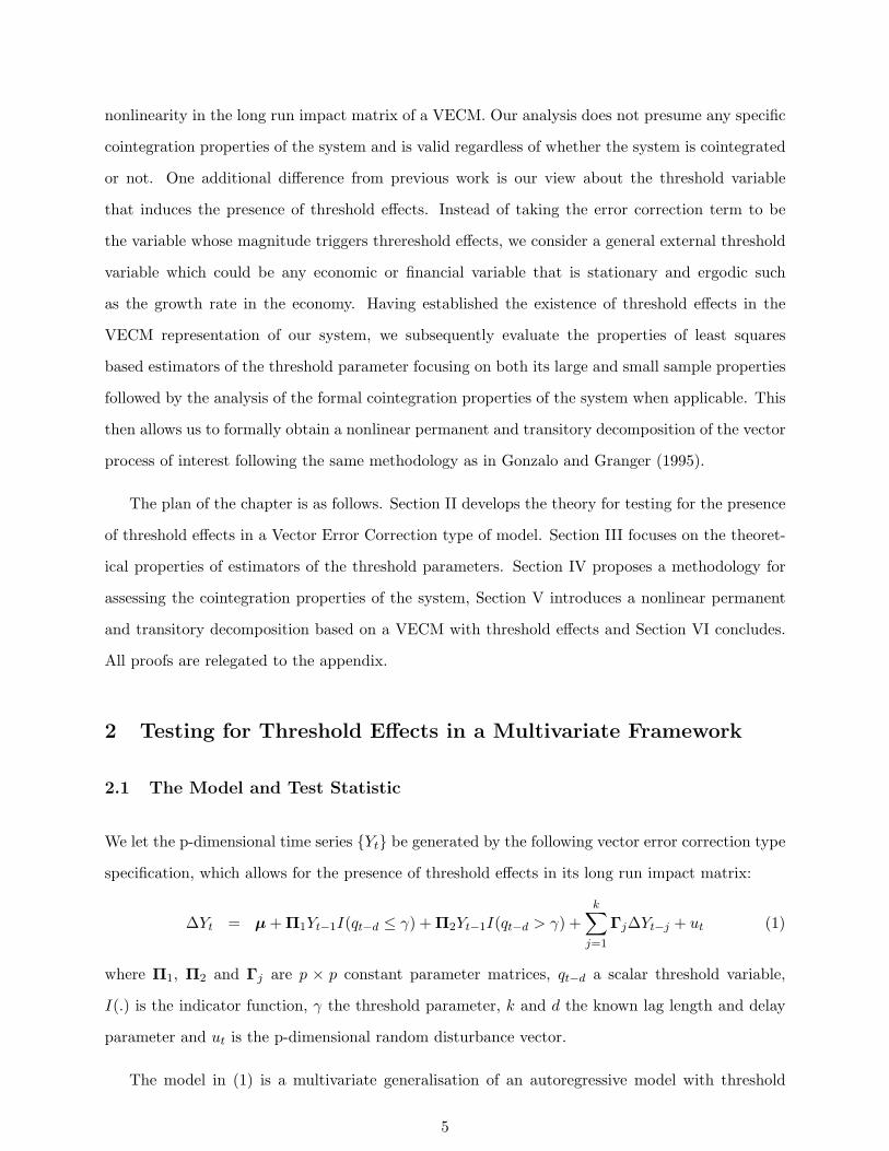
We let the p-dimensional time series Yt be generated by the following vector error correction type

specification, which allows for the presence of threshold effects in its long run impact matrix:

∆Yt = µ + Π1Yt−1I(qt−d ≤ γ) + Π2Yt−1I(qt−d > γ) +k∑

j=1

Γj∆Yt−j + ut (1)

where Π1, Π2 and Γj are p × p constant parameter matrices, qt−d a scalar threshold variable,

I(.) is the indicator function, γ the threshold parameter, k and d the known lag length and delay

parameter and ut is the p-dimensional random disturbance vector.

The model in (1) is a multivariate generalisation of an autoregressive model with threshold

5

effects whose dynamics are characterised by piecewise linear vector autoregressions. The regime

switches are governed by the magnitude of the threshold variable qt crossing an unknown threshold

value γ. The specification in (1) is similar to the one considered in Seo (2004) with the difference

that no assumptions are made about the rank structure of either Π1 or Π2, and the threshold

variable is not necessarily given by the error correction term such as qt = β′Yt with β denoting the

single cointegrating vector for instance.

The initial question of interest in the context of the specification in (1) is whether the long run

impact matrix is truly characterised by threshold effects driven by the threshold variable qt. Under

the absence of such effects we have a standard linear VECM with Π1 = Π2 and this restriction

can be tested via a conventional Wald type test statistic against the alternative H1 : Π1 6= Π2.

At this stage it is important to note that the sole purpose of testing the above null hypothesis

is to uncover the presence or absence of threshold effects in the long run impact matrix. More

importantly we wish to conduct this set of inferences regardless of the stationarity properties of

Yt, in the sense that our null hypothesis may hold under a purely stationary set up or a unit

root set up with or without cointegration. If the null hypothesis is not rejected we can then

carry on with the process of exploring the stochastic properties of the data following for instance

Johansen’s methodology (see Johansen (1998) and references therein). Before proceeding further

and to motivate our working model we consider two simple examples illustrating particular cases

of our specification in (1).

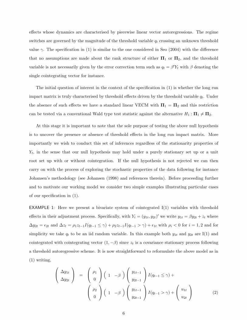
EXAMPLE 1: Here we present a bivariate system of cointegrated I(1) variables with threshold

effects in their adjustment process. Specifically, with Yt = (y1t, y2t)′ we write y1t = βy2t + zt where

∆y2t = ε2t and ∆zt = ρ1zt−1I(qt−1 ≤ γ) + ρ2zt−1I(qt−1 > γ) + ε1t with ρi < 0 for i = 1, 2 and for

simplicity we take qt to be an iid random variable. In this example both y1t and y2t are I(1) and

cointegrated with cointegrating vector (1,−β) since zt is a covariance stationary process following

a threshold autoregressive scheme. It is now straightforward to reformulate the above model as in

(1) writing, ∆y1t

∆y2t

=

ρ1

0

(1 −β

) y1t−1

y2t−1

I(qt−1 ≤ γ) +

ρ2

0

(1 −β

) y1t−1

y2t−1

I(qt−1 > γ) +

u1t

u2t

(2)

6

with u1t = ε1t + βε2t and u2t = ε2t.

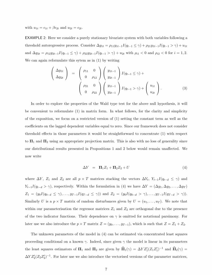
EXAMPLE 2: Here we consider a purely stationary bivariate system with both variables following a

threshold autoregressive process. Consider ∆y1t = ρ11y1t−1I(qt−1 ≤ γ) + ρ21y1t−1I(qt−1 > γ) + u1t

and ∆y2t = ρ12y2t−1I(qt−1 ≤ γ) + ρ22y2t−1I(qt−1 > γ) + u2t with ρi1 < 0 and ρi2 < 0 for i = 1, 2.

We can again reformulate this sytem as in (1) by writing ∆y1t

∆y2t

=

ρ11 0

0 ρ12

y1t−1

y2t−1

I(qt−1 ≤ γ) +

ρ21 0

0 ρ22

y1t−1

y2t−1

I(qt−1 > γ) +

u1t

u2t

. (3)

In order to explore the properties of the Wald type test for the above null hypothesis, it will

be convenient to reformulate (1) in matrix form. In what follows, for the clarity and simplicity

of the exposition, we focus on a restricted version of (1) setting the constant term as well as the

coefficients on the lagged dependent variables equal to zero. Since our framework does not consider

threshold effects in those parameters it would be straightforward to concentrate (1) with respect

to Π1 and Π2 using an appropriate projection matrix. This is also with no loss of generality since

our distributional results presented in Propositions 1 and 2 below would remain unaffected. We

now write

∆Y = Π1Z1 + Π2Z2 + U (4)

where ∆Y , Z1 and Z2 are all p × T matrices stacking the vectors ∆Yt, Yt−1I(qt−d ≤ γ) and

Yt−1I(qt−d > γ), respectively. Within the formulation in (4) we have ∆Y = (∆y1, ∆y2, . . . ,∆yT )

Z1 = (y0I(q0−d ≤ γ), . . . , yT−1I(qT−d ≤ γ)) and Z2 = (y0I(q0−d > γ), . . . , yT−1I(qT−d > γ)).

Similarly U is a p × T matrix of random disturbances given by U = (u1, . . . , uT ). We note that

within our parameterisation the regressor matrices Z1 and Z2 are orthogonal due to the presence

of the two indicator functions. Their dependence on γ is omitted for notational parsimony. For

later use we also introduce the p× T matrix Z = (y0, . . . , yT−1), which is such that Z = Z1 + Z2.

The unknown parameters of the model in (4) can be estimated via concentrated least squares

proceeding conditional on a known γ. Indeed, since given γ the model is linear in its parameters

the least squares estimators of Π1 and Π2 are given by Π1(γ) = ∆Y Z ′1(Z1Z′1)−1 and Π2(γ) =

∆Y Z ′2(Z2Z′2)−1. For later use we also introduce the vectorised versions of the parameter matrices,

7

writing π1 ≡ vec Π1 and π2 ≡ vec Π2, and the null hypothesis of interest can be equivalently

expressed as H0 : π1 = π2 or H0 : Rπ = 0 with R = [Ip2 ,−Ip2 ] and π = (π′1, π′2)′.

The Wald statistic for testing the above null hypothesis takes the following form

WT (γ) = (Rπ)′[R((DD′)−1 ⊗ Ωu)R′

]−1(Rπ) (5)

where ⊗ is the Kronecker product operator, π1 = [(Z1Z′1)−1Z1 ⊗ Ip]vec ∆Y , π2 = [(Z2Z

′2)−1Z2 ⊗

Ip]vec ∆Y and D = [Z1 Z2]. The p × p matrix Ωu refers to the least squares estimator of the

covariance matrix defined as Ωu = U U ′/T with U = ∆Y − Π1(γ)Z1 − Π2(γ)Z2. Since Z1 and

Z2 are orthogonal it also immediately follows that DD′ = diag(Z1Z′1, Z2Z

′2) and (DD′)−1 ⊗ Ωu =

diag[(Z1Z′1)−1 ⊗ Ωu, (Z2Z

′2)−1 ⊗ Ωu]. We can thus also reformulate the Wald statistic in (5) as

WT (γ) = (π1 − π2)′[(Z2Z

′2)(ZZ ′)−1(Z1Z

′1)⊗ Ω−1

u

](π1 − π2) (6)

where ZZ ′ = Z1Z′1 + Z2Z

′2.

At this stage it is also important to reiterate the fact that when implementing our test of the

null hypothesis of linearity with say Π1 = Π2 = Π, the corresponding characteristic polynomial

Φ(z) = (1− z)Ip −Πz will be assumed to have all its roots either outside or on the unit circle and

the number of unit roots present in the system will be given by p− r with 0 ≤ r ≤ p. Our analysis

rules out instances of explosive behaviour or processes that may be integrated of order two. This

also allows us to have a direct correspondence between the stochastic properties of Yt under the

null hypothesis and the rank structure of the long run impact matrix Π. In the particular case

where all the roots of the characteristic polynomial are outside the unit circle, the series will be

referred to as I(0).

2.2 Assumptions and Limiting Distributions

Throughout this section we will be operating under the following set of assumptions

(A1) ut = (u1t, . . . , upt)′ is a zero mean iid sequence of p dimensional random vectors with a

bounded density function, covariance matrix E[utu′t] = Ωu > 0 and with E|uit|2δ < ∞ for

some δ > 2 and i = 1, . . . , p;

(A2) qt is a strictly stationary and ergodic sequence that is independent of uis ∀t, s, i = 1, . . . , p

and has distribution function F that is continuous everywhere;

8

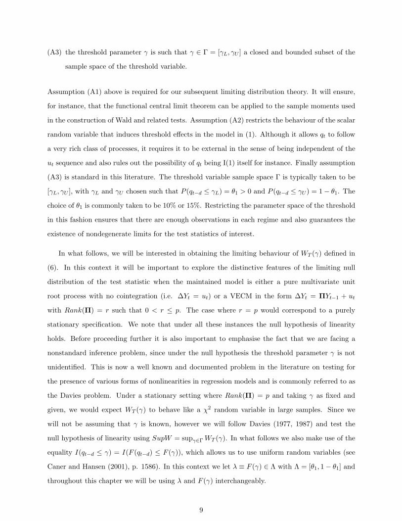
(A3) the threshold parameter γ is such that γ ∈ Γ = [γL, γU ] a closed and bounded subset of the

sample space of the threshold variable.

Assumption (A1) above is required for our subsequent limiting distribution theory. It will ensure,

for instance, that the functional central limit theorem can be applied to the sample moments used

in the construction of Wald and related tests. Assumption (A2) restricts the behaviour of the scalar

random variable that induces threshold effects in the model in (1). Although it allows qt to follow

a very rich class of processes, it requires it to be external in the sense of being independent of the

ut sequence and also rules out the possibility of qt being I(1) itself for instance. Finally assumption

(A3) is standard in this literature. The threshold variable sample space Γ is typically taken to be

[γL, γU ], with γL and γU chosen such that P (qt−d ≤ γL) = θ1 > 0 and P (qt−d ≤ γU ) = 1− θ1. The

choice of θ1 is commonly taken to be 10% or 15%. Restricting the parameter space of the threshold

in this fashion ensures that there are enough observations in each regime and also guarantees the

existence of nondegenerate limits for the test statistics of interest.

In what follows, we will be interested in obtaining the limiting behaviour of WT (γ) defined in

(6). In this context it will be important to explore the distinctive features of the limiting null

distribution of the test statistic when the maintained model is either a pure multivariate unit

root process with no cointegration (i.e. ∆Yt = ut) or a VECM in the form ∆Yt = ΠYt−1 + ut

with Rank(Π) = r such that 0 < r ≤ p. The case where r = p would correspond to a purely

stationary specification. We note that under all these instances the null hypothesis of linearity

holds. Before proceeding further it is also important to emphasise the fact that we are facing a

nonstandard inference problem, since under the null hypothesis the threshold parameter γ is not

unidentified. This is now a well known and documented problem in the literature on testing for

the presence of various forms of nonlinearities in regression models and is commonly referred to as

the Davies problem. Under a stationary setting where Rank(Π) = p and taking γ as fixed and

given, we would expect WT (γ) to behave like a χ2 random variable in large samples. Since we

will not be assuming that γ is known, however we will follow Davies (1977, 1987) and test the

null hypothesis of linearity using SupW = supγ∈Γ WT (γ). In what follows we also make use of the

equality I(qt−d ≤ γ) = I(F (qt−d) ≤ F (γ)), which allows us to use uniform random variables (see

Caner and Hansen (2001), p. 1586). In this context we let λ ≡ F (γ) ∈ Λ with Λ = [θ1, 1− θ1] and

throughout this chapter we will be using λ and F (γ) interchangeably.

9

In the following proposition we summarise the limiting behaviour of the Wald statistic for testing

the null hypothesis of linearity when it is assumed that the system is purely stationary.

Proposition 1 Under assumptions A1-A3, H0 : Π1 = Π2 and Yt a p-dimensional I(0) vector we

have

SupW ⇒ Supλ∈ΛG(λ)′V (λ)−1G(λ) (7)

where G(λ) is a zero mean p2-dimensional Gaussian random vector with covariance E[G(λ1)G(λ2)] =

V (λ1 ∧ λ2) and V (λ) = λ(1− λ)(Q⊗ Ωu) with Q = E[ZZ ′].

REMARK 1: It is interesting to note that the above limiting distribution is equivalent to a normalised

squared Brownian Bridge process identical to the one arising when testing for the presence of

structural breaks as in Andrews (1993, Theorem 3, p. 838). The same distribution also arises in

particular parameterisations of self-exciting threshold autoregressive models when only the constant

terms are allowed to be different in each regime (see Chan (1990)). We also note that for known and

given γ, the quantity G(λ)′V (λ)−1G(λ) reduces to a χ2 random variable with p2 degrees of freedom.

Since G(λ) is (Q⊗ Ωu)12 N(0, λ(1− λ)Ip2) ≡ (Q⊗ Ωu)

12 [W (λ)− λW (1)], with W (.) denoting a p2-

dimensional standard Brownian Motion, the result follows from the above definition of V (λ). We

also note that the limiting process is free of nuisance parameters, solely depending on the number

of parameters being tested under the null hypothesis and is tabulated in Andrews (1993, Table 1,

p. 840). For a more extensive set of p-values of the corresponding limiting distributions see also

Hansen (1997).

In the next proposition we summarise the limiting behaviour of the same Wald test statistic

when the system is assumed to be a p-dimensional pure I(1) process as ∆Yt = ut or alternatively

I(1) but cointegrated as in ∆Yt = αβ′Yt−1 + ut, with α and β having reduced ranks. In what

follows a standard Brownian Sheet W (s, t) is defined as a zero mean two-parameter Gaussian

process indexed by [0, 1]2 and having a covariance function given by Cov[W (s1, t1),W (s2, t2)] =

(s1 ∧ t1)(s2 ∧ t2) while a Kiefer process K on [0, 1]2 is given by K(s, t) = W (s, t) − tW (s, 1). The

Kiefer process is also a two-parameter Gaussian process with zero mean and covariance function

Cov[K(s1, t1),K(s2, t2)] = (s1 ∧ s2)(t1 ∧ t2 − t1t2).

10

Proposition 2 Under assumptions A1-A3, H0 : Π1 = Π2 and Yt a p-dimensional I(1) vector

cointegrated or not:

SupW ⇒ Supλ∈Λ1

λ(1− λ)tr

(∫ 1

0W (r)dK(r, λ)′

)′(∫ 1

0W (r)W (r)′

)−1

(∫ 1

0W (r)dK(r, λ)′

)(8)

where K(r, λ) is a Kiefer process given by K(r, λ) = W (r, λ) − λW (r, 1) with W (.) denoting a

p-dimensional standard Brownian Motion and W (r, λ) a p-dimensional standard Brownian Sheet.

Looking at the expression of the limiting distribution in Proposition 2, we again observe that

for given and known λ the limiting random variable is χ2(p2) exactly as occurred under the

purely stationary setup of proposition 1. This follows from the observation that W (r) and K(r, λ)

are independent. Note that we have E[W (r)K(r, λ)] = E[W (r)W (r, λ)] − λE[W (r)2] and since

E[W (r)W (r, λ)] = rλ and E[W (r)2] = r the result follows. It also follows that the limiting random

variables in (7) and (8) are equivalent in distribution.

2.3 Simulation Based Evidence

Having established the limiting behaviour of the Wald statistic for testing the null of no threshold

effects within the VECM type representation we next explore the adequacy of the asymptotic

approximations presented in Propositions 1-2 when dealing with finite samples. This will also

allow us to explore the documented robustness of the above limiting distributions to the absence or

presence of unit roots and cointegration, and to the stochastic properties of the threshold variable

qt when faced with limited sample sizes.

We initially consider a purely stationary bivariate DGP, as the model under the null hypothesis,

parameterised as Yt = ΦYt−1 + ut with Φ = diag(0.5, 0.8) and ut = NID(0, I2). As a candidate

threshold variable required in the construction of the Wald statistic we consider two options. One

in which qt is taken to be a normal iid random variable (independent of uit, i = 1, 2) and one where

qt follows a stationary AR(1) process given by qt = θqt−1 + εt with θ = 0.5 and εt = NID(0, 1)

with Cov(εt, uis) = 0 ∀t, s and i = 1, 2. Regarding the magnitude of the delay parameter we

set d = 1 throughout all our experiments, all conducted using samples of size T = 200, 400, 2000

across N = 5000 replications and with a 10% trimming of the sample space of the threshold

variable. Another important purpose of our experiments is to construct a range of critical values

11

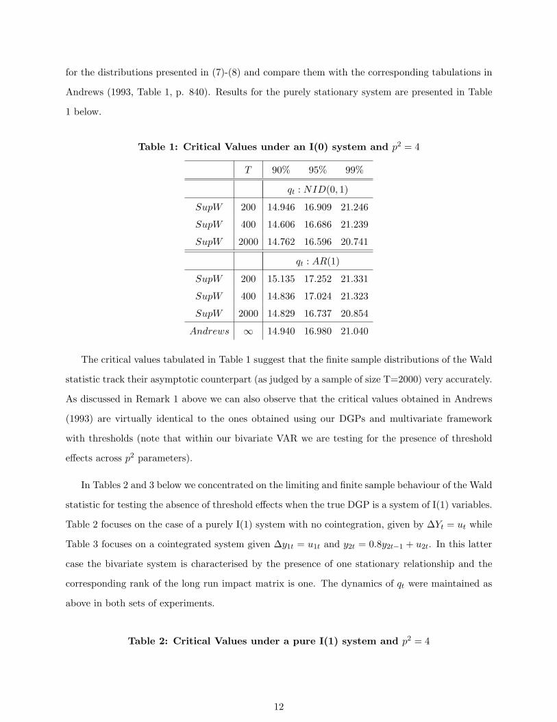
for the distributions presented in (7)-(8) and compare them with the corresponding tabulations in

Andrews (1993, Table 1, p. 840). Results for the purely stationary system are presented in Table

1 below.

Table 1: Critical Values under an I(0) system and p2 = 4

T 90% 95% 99%

qt : NID(0, 1)

SupW 200 14.946 16.909 21.246

SupW 400 14.606 16.686 21.239

SupW 2000 14.762 16.596 20.741

qt : AR(1)

SupW 200 15.135 17.252 21.331

SupW 400 14.836 17.024 21.323

SupW 2000 14.829 16.737 20.854

Andrews ∞ 14.940 16.980 21.040

The critical values tabulated in Table 1 suggest that the finite sample distributions of the Wald

statistic track their asymptotic counterpart (as judged by a sample of size T=2000) very accurately.

As discussed in Remark 1 above we can also observe that the critical values obtained in Andrews

(1993) are virtually identical to the ones obtained using our DGPs and multivariate framework

with thresholds (note that within our bivariate VAR we are testing for the presence of threshold

effects across p2 parameters).

In Tables 2 and 3 below we concentrated on the limiting and finite sample behaviour of the Wald

statistic for testing the absence of threshold effects when the true DGP is a system of I(1) variables.

Table 2 focuses on the case of a purely I(1) system with no cointegration, given by ∆Yt = ut while

Table 3 focuses on a cointegrated system given ∆y1t = u1t and y2t = 0.8y2t−1 + u2t. In this latter

case the bivariate system is characterised by the presence of one stationary relationship and the

corresponding rank of the long run impact matrix is one. The dynamics of qt were maintained as

above in both sets of experiments.

Table 2: Critical Values under a pure I(1) system and p2 = 4

12

T 90% 95% 99%

qt : NID(0, 1)

SupW 200 14.970 17.023 22.098

SupW 400 14.858 18.578 21.205

SupW 2000 15.012 16.947 20.967

qt : AR(1)

SupW 200 15.369 17.197 22.164

SupW 400 14.948 18.527 21.358

SupW 2000 14.904 16.840 21.212

Andrews ∞ 14.940 16.980 21.040

Table 3: Critical Values under a cointegrated system and p2 = 4

T 90% 95% 99%

qt : NID(0, 1)

SupW 200 15.030 17.236 21.431

SupW 400 14.685 16.879 20.926

SupW 2000 14.723 16.739 20.911

qt : AR(1)

SupW 200 15.068 16.903 21.074

SupW 400 15.150 17.040 21.153

SupW 2000 14.961 16.758 21.013

Andrews ∞ 14.940 16.980 21.040

The empirical results presented in Tables 2-3 above clearly illustrate the robustness of the

limiting distributions to various parameterisations of the threshold variable. Our tabulations also

corroborate our earlier observation that the limiting distributions are unaffected by the presence

or absence of I(1) components.

3 Estimation of the Threshold Parameter

Once inferences based on the Wald test reject the null hypothesis of a linear VECM our next

objective is to obtain a consistent estimator of the threshold parameter. The model under which

we operate is now given by ∆Y = Π1Z1 + Π2Z2 + U . We propose to obtain an estimator of γ

13

based on the least squares principle. Letting U(γ) = ∆Y − Π1(γ)Z1(γ)− Π2(γ)Z2(γ) we consider

γ = arg minγ∈Γ

|U(γ)U(γ)′|. (9)

Before establishing the large sample behaviour of γ introduced in (9) it is important to highlight the

fact that a VECM type of representation with threshold effects as in (4) is compatible with either

a purely stationary Yt or a system of I(1) variables that is cointegrated in a conventional sense and

with threshold effects present in its adjustment process. Examples of such processes are provided

in (2) and (3) above while a formal discussion of the stationarity properties of Yt generated from

(4) is provided below.

The following proposition summarises the limiting behaviour of the threshold parameter esti-

mator defined above with γ0 referring to its true magnitude.

Proposition 3 Under assumptions (A1)-(A3) with Yt I(0) or I(1) but cointegrated and generated

as in (4) we have γp→ γ0 as T →∞.

From the above proposition it is clear that the consistency property of the threshold parameter

estimator remains unaffected by the presence of I(1) components. In order to empirically illustrate

the above proposition, and explore the behaviour of γ in smaller samples, we conducted a Monte-

Carlo experiment covering a range of parameterisations including purely stationary and cointegrated

systems. Our objective was to assess the finite sample performance of the least squares based

estimator of γ0 in moderate to large samples in terms of bias and variability.

For the purely stationary case we consider the specification introduced in (3), setting (ρ11, ρ21) =

(−0.8,−0.4) and (ρ12, ρ22) = (−0.2,−0.6). Regarding the choice of threshold variable we consider

the case of a purely Gaussian iid process as well as an AR(1) specification given by qt = 0.5qt−1 +ut

with ut = NID(0, 1). The true threshold parameter is set to γ0 = 0.25 under the AR(1) dynamics

and to γ0 = 0 when qt is iid. The delay parameter is fixed at d = 1. For the cointegrated

case we consider a system given by y1t = 2y2t + zt with ∆y2t = ε2t and zt = 0.2zt−1I(qt−1 ≤γ0) + 0.8zt−1I(qt−1 > γ0) + νt, while retaining the same dynamics for qt and the same threshold

parameter configurations as above. Both ε2t and νt are chosen as NID(0,1) random variables.

Results for these two classes of DGPs are presented in Table 4 below, which displays the

empirical mean and standard deviation of γ estimated as in (9) using samples of size T = 200 and

T = 400 across N = 5000 replications.

14

Table 4: Empirical Mean and Standard Deviation of γ

qt AR(1), γ0 = 0.15 qt iid, γ0 = 0

E(γ) Std(γ) E(γ) Std(γ)

Stationary System

T = 200 0.142 0.278 −0.014 0.247

T = 400 0.145 0.108 −0.004 0.100

Cointegrated System

T = 200 0.140 0.266 −0.006 0.229

T = 400 0.144 0.101 −0.003 0.091

From both of the above experiments we note that γ as defined in (9) displays a reasonably small

and negative finite sample bias of approximately 0.5% under both configurations of the dynamics

of the threshold variable and system properties. At the same time, however, we note that γ is

characterised by a substantial variability across all model configurations. Its empirical standard

deviation is virtually twice the magnitude of γ0 under T=200 and, although clearly declining with

the sample size, remains substantial even under T=400. Similar features of threshold parameter

estimators have also been documented in Gonzalo and Pitarakis (2002).

Taking the presence of threshold effects as given together with the availability of a consistent

estimator of the unknown threshold parameter, our next concern is to explore further the stochastic

properties of the p-dimensional vector Yt.

4 Stochastic Properties of the System and Rank Configuration of

the VECM with Threshold Effects

So far the test developed in the previous sections allows us to decide whether the inclusion of

threshold effects into a VECM type specification is supported by the data. Given the simplicity

of its implementation, and the fact that the limiting distribution of the test statistic is unaffected

by the stationarity properties of the variables being modelled, the proposed Wald based inferences

can be viewed as a useful pre-test before implementing a formal analysis of the integration and

cointegration properties of the system. If the null hypothesis is not rejected for instance we can

proceed with the specification of a linear VECM using for instance the methodology developed in

Johansen (1995 and references therein).

15

Our next concern is to explore the implications of the rejection of the null hypothesis of linearity

for the stability and, when applicable, cointegration properties of Yt whose dynamics are now known

to be described by the specification in (4). Although rejecting the hypothesis that Π1 = Π2 rules

out the scenario of a purely I(1) system with no cointegration as traditionally defined, since having

Π1 6= Π2 is trivially incompatible with the specification ∆Y = U , as shown below, it remains

possible that the system is either purely covariance stationary or I(1) with cointegration in a sense

to be made clear (see for instance the formulation in (2) under example 1).

4.1 Stability Properties of the System

In the context of our specification in (4), and maintaining the notation Φ1 = Ip + Π1 and Φ2 =

Ip + Π2 so that the system can be formulated as Yt = ΦtYt−1 + ut with Φt = Φ1I(qt−d ≤ γ) +

Φ2I(qt−d > γ), the stability properties of the system are summarised in the following proposition

where for a square matrix M the notation ρ(M) refers its spectral radius.

Proposition 4 Under assumptions (A1)-(A3), Yt generated from (4) is covariance stationary iff

ρ(F (γ)(Φ1 ⊗Φ1) + (1− F (γ))(Φ2 ⊗Φ2)) < 1.

From the above proposition it is interesting to note that even if one of the two regimes has a root

on the unit circle the model could still be covariance stationary. In fact the system could even be

characterised by an explosive behaviour in one of its regimes while still being covariance stationary,

if for instance the magnitudes of the transition probabilities are such that switching occurs very

often. Note also that the condition ensuring the covariance stationarity of Yt is also equivalent to

requiring the eigenvalues of E[Φt ⊗Φt] to have moduli less than one.

EXAMPLE 3: We can here consider the example of a bivariate process given by Yt = I2Yt−1I(qt−d ≤γ) + Φ2Yt−1I(qt−d > γ) + ut and let Φ2 = φI2 with |φ| < 1 where I2 denotes a two dimensional

identity matrix. This system can be seen to be characterised by a random walk type of behaviour

in one regime and is covariance stationary in the second regime. In matrix form we have ∆y1t

∆y2t

=

0 0

0 0

y1t−1

y2t−1

I(qt−1 ≤ γ) +

φ− 1 0

0 φ− 1

y1t−1

y2t−1

I(qt−1 > γ) +

ε1t

ε2t

. (10)

16

Letting M = F (γ)(Φ1 ⊗ Φ1) + (1 − F (γ))(Φ2 ⊗ Φ2)), it is straightforward to establish that in

the case of (10) we have ρ(M) = F (γ) + φ2(1 − F (γ)) < 1, since φ2 < 1 and thus implying that

Yt = (y1t, y2t)′ is covariance stationary.

EXAMPLE 4: Another example of a covariance stationary system is given by ∆y1t

∆y2t

=

0 0

0 φ− 1

y1t−1

y2t−1

I(qt−1 ≤ γ) +

φ− 1 0

0 0

y1t−1

y2t−1

I(qt−1 > γ) +

ε1t

ε2t

(11)

for which we have ρ(M) = (1 − F (γ))(1 − φ)2 < 1 if F (γ) < 0.5, and ρ(M) = F (γ)(1 − φ)2 <

1 if F (γ) > 0.5. On the other hand, if we concentrate on the specification given in (2), it is

straighforward to establish that ρ(M) = 1 thus violating the requirement for Yt to be covariance

stationary.

For later use it is also important at this stage to observe the correspondence between the ranks

of the long run impact matrices presented in the above examples and the covariance stationarity of

each system. In example 3, for instance, we note that r1 ≡ Rank(Π1) = 0 and r2 ≡ Rank(Π2) = 2,

while in model (11) we have (r1, r2) = (1, 1). This highlights the fact that within a nonlinear

specification, as in (4), the correspondence between the rank structure of the long run impact

matrices and the stability/cointegration properties of the system will be less clearcut than within

a simple linear VECM. Before exploring further this issue it will be important to clarify the type

of threshold nonlinearities that are compatible with an I(1) system and its VECM representation

in (4).

4.2 I(1)’ness and Cointegration within a nonlinear VECM

The recent literature on the inclusion of nonlinear features in models with I(1) variables and coin-

tegration can typically be categorised into two strands. Single equation approaches, which aim to

detect the presence of nonlinearities in regressions with I(1) processes known to be cointegrated

(see Saikkonen and Choi (2004), Hong (2003), Arai (2004)). In Saikkonen and Choi (2004), for

instance, the authors included a smooth transition type of function g(.) within a postulated coin-

tegrating regression model of the form y1t = βy2t + θy2t g(y2t; γ) + ut and proposed a methodology

for testing the null hypothesis of no such effects given here by H0 : θ = 0. The presence of such

17

nonlinearities within a cointegrating relationship implies some form of switching equilibria in the

sense that the cointegrating vector is allowed to be different depending on the magnitude of y2t.

In both Hong (2003) and Arai (2004), the authors focused on a similar setup without an explicit

choice of functional form. This was achieved through the inclusion of additional polynomial terms

in the y2 variable in the right hand side of a cointegrating regression.

Another strand of the same literature focused on the treatment of nonlinearities within a mul-

tivariate error correction framework. The motivation underlying this research was again to detect

the presence of nonlinear cointegration, but here defined as a nonlinear adjustment towards the

long run equilibrium while maintaining the assumption that the cointegration relationship is itself

linear. Another important maintained assumption in this line of research is the existence of a single

cointegrating vector (see Balke and Fomby (1997), Seo and Hansen (2002), Seo (2004)). Regarding

the theoretical properties of multivariate models with nonlinearities, Bec and Rahbek (2004) have

explored the strict stationarity and ergodicity properties of multivariate error correction models

with general cointegrating rank and nonlinearities in their adjustment process.

One aspect that seems not to have been emphasised in the literature is the fact that, when

operating within a VECM type framework, an important aspect of restricting the presence of

nonlinearity to occur solely in the adjustment process stems from representation concerns. More

specifically it can be shown that two I(1) variables that are linearly cointegrated but with a nonlinear

adjustment process continue to admit a “nonlinear” VECM representation similar to (4) above.

If we also wish to explore the possibility of nonlinearities in the cointegrating relationship itself

however it becomes difficult to justify the existence of a VECM representation a la Granger.

To highlight this point let us consider the following simple nonlinear cointegrating relationship

which is characterised by the presence of a threshold type of nonlinearity

y1t = βy2t + θy2tI(qt−1 > γ) + zt

∆y2t = ε2t

∆zt = ρzt−1 + ut. (12)

with ρ < 0 and zt representing the stationary equilibrium error.

If we were in a linear setup with θ = 0 it would be straightforward to reformulate the above

specification as ∆y1t = ρzt−1 + νt, with νt = ut + βε2t, and we would have a traditional VECM

18

representation with ρ playing the role of the adjustment coefficient to equilibrium and zt−1 =

(y1t−1 − βy2t−1) denoting the previous period’s equilibrium error. At this stage it is important to

note that a key aspect of the linear setup that allows us to move towards an ECM type representation

is the fact that taking y2t to be an I(1) variable, as in (12), directly implies that y1t is also difference

stationary since taking the first difference of both sides of the first equation gives ∆y1t = β∆y2t+∆zt

and both the left and right hand side are characterised by the same integration properties.

When we introduce nonlinearities in the relationship linking y1t and y2t, however, the stochas-

tic properties of the system become less obvious. Specifically, taking y2t to be I(1) or equivalently

difference stationary no longer implies that y1t is also difference stationary. Indeed, it becomes

straightforward to show that although the I(1)’ness of y2t makes y1t nonstationary this nonstation-

arity of y1t can no longer be removed by first differencing. Differently put, although the variance

of y1t behaves in a manner similar to the variance of a random walk, first differencing y1t will no

longer make it stationary. More formally, if we take the first difference of the first equation in (12)

and using the notation It ≡ I(qt > γ) we have

∆y1t = β∆y2t + θ∆(y2tIt−1) + ∆zt

= ρzt−1 + θy2t−1∆It−1 + νt (13)

where νt = θε2tIt−1 + βε2t + ut. Clearly the presence of the term y2t−1∆It, in the right hand

side of (13) precludes the possibility of a traditional ECM type representation a la Granger. If

we take qt to be an iid process for instance it is straightforward to establish that V (y2t−1∆It) =

2F (γ)(1 − F (γ))(t − 1). Similarly, y1t cannot really be viewed as a difference stationary process

as would have been the case within a linear framework. As dicussed in Granger, Inoue and Morin

(1997), where the authors introduced a specification similar to (13), the correct but not directly

operational form of the error correction model could be formulated as

∆y1t − θy2t−1∆It−1 = ρzt−1 + νt

where now both the left and right hand side components are stationary. Practical tools and their

theoretical properties for handling models such as the above are developed in Gonzalo and Pitarakis

(2005a).

Our specification in (13) has highlighted the difficulties of handling switching phenomena within

the cointegrating relationship itself if we want to operate within the traditional VECM framework.

19

It is also worth emphasising that similar conceptual difficulties will arise in non-VECM based

approaches to the treatment of nonlinearities in cointegrating relationships. Writing y1t = βty2t+ut,

with y2t an I(1) variable and ut an I(0) error term, defines a stationary relationship between y1t

and y2t which is not invalid per se. However, it would be inaccurate to refer to it as a cointegrating

relationship linking two I(1) variables since y1t cannot be difference stationary due to the time

varying nature of βt.

In summary, a system such as (12) which has a switching cointegrating vector cannot admit a

VECM representation as in (4) in which both the left and right hand sides are balanced in the sense

of both being stationary. Equivalently, for an I(1) vector to admit a formal VECM representation

as in (4) it must be the case that the threshold effects are solely present in the adjustment process.

4.3 Rank Configuration under Alternative Stochastic Properties of Yt

Our objective here is to further explore the correspondence between the rank characteristics of Π1

and Π2 and the stability properties of Yt akin to the well known relationship between the rank

of the long run impact matrix of a linear VECM specification and its cointegration properties.

We are interested for instance in the rank configurations of Π1 and Π2 that are consistent with

covariance stationarity of Yt. Similarly, we also wish to explore the correspondence between the

presence of threshold effects in the adjustment process of a cointegrated I(1) system and the rank

configurations of the two long run impact matrices that are compatible with such a system.

Within a linear VECM specification, whose corresponding lag polynomial has roots either on

or outside the unit circle, it is well known that having matrix Π that has full rank also implies

that the underlying process is I(0). Although, from our result in proposition 4 it is straightforward

to see that if both or either of Π1 and Π2 have full rank then Yt generated from (4) is going

to be covariance stationary as well, it is also true that the full rank condition is not necessary for

covariance stationarity. Our examples in (2) and (11), for instance, have illustrated the fact that two

identical rank configurations, say (r1, r2) = (1, 1) may be compatible with either a purely I(1) system

as in (2) or a covariance stationary system as in (11). Similarly, example 3 with (r1, r2) = (0, 2)

illustrated the possibility of having a covariance stationary DGP in which either Π1 or Π2 have

zero rank. These observations highlight the difficulties that may arise when attempting to clearly

define the meaning of “nonlinear cointegration” when operating within an Error Correction type

20

of model.

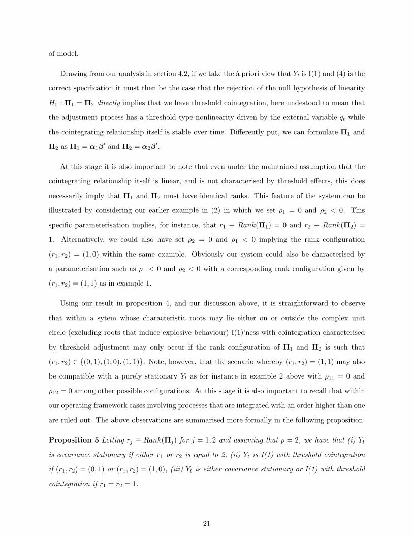
Drawing from our analysis in section 4.2, if we take the a priori view that Yt is I(1) and (4) is the

correct specification it must then be the case that the rejection of the null hypothesis of linearity

H0 : Π1 = Π2 directly implies that we have threshold cointegration, here undestood to mean that

the adjustment process has a threshold type nonlinearity driven by the external variable qt while

the cointegrating relationship itself is stable over time. Differently put, we can formulate Π1 and

Π2 as Π1 = α1β′ and Π2 = α2β

′.

At this stage it is also important to note that even under the maintained assumption that the

cointegrating relationship itself is linear, and is not characterised by threshold effects, this does

necessarily imply that Π1 and Π2 must have identical ranks. This feature of the system can be

illustrated by considering our earlier example in (2) in which we set ρ1 = 0 and ρ2 < 0. This

specific parameterisation implies, for instance, that r1 ≡ Rank(Π1) = 0 and r2 ≡ Rank(Π2) =

1. Alternatively, we could also have set ρ2 = 0 and ρ1 < 0 implying the rank configuration

(r1, r2) = (1, 0) within the same example. Obviously our system could also be characterised by

a parameterisation such as ρ1 < 0 and ρ2 < 0 with a corresponding rank configuration given by

(r1, r2) = (1, 1) as in example 1.

Using our result in proposition 4, and our discussion above, it is straightforward to observe

that within a sytem whose characteristic roots may lie either on or outside the complex unit

circle (excluding roots that induce explosive behaviour) I(1)’ness with cointegration characterised

by threshold adjustment may only occur if the rank configuration of Π1 and Π2 is such that

(r1, r2) ∈ (0, 1), (1, 0), (1, 1). Note, however, that the scenario whereby (r1, r2) = (1, 1) may also

be compatible with a purely stationary Yt as for instance in example 2 above with ρ11 = 0 and

ρ12 = 0 among other possible configurations. At this stage it is also important to recall that within

our operating framework cases involving processes that are integrated with an order higher than one

are ruled out. The above observations are summarised more formally in the following proposition.

Proposition 5 Letting rj ≡ Rank(Πj) for j = 1, 2 and assuming that p = 2, we have that (i) Yt

is covariance stationary if either r1 or r2 is equal to 2, (ii) Yt is I(1) with threshold cointegration

if (r1, r2) = (0, 1) or (r1, r2) = (1, 0), (iii) Yt is either covariance stationary or I(1) with threshold

cointegration if r1 = r2 = 1.

21

According to the above proposition, even if at most one of the two long run impact matrices

characterising the model in (4) is found to have full rank it must be that Yt itself is covariance

stationary. On the other hand if we have a rank configuration such as (r1, r2) = (0, 1) or (r1, r2) =

(1, 0) then this would imply that Yt described by (4) is I(1) and the model is characterised by

threshold effects in its adjustment process towards its long run equilibrium. Intuitively, such a

rank configuration captures the idea of an adjustment process that shuts off when the threshold

variable qt crosses above or below a certain magnitude given by γ. Finally, the case whereby

(r1, r2) = (1, 1) is compatible with either a purely covariance stationary system or an I(1) system

with an underlying adjustment process characterised by different speeds of adjustment depending

on the magnitude of qt.

4.4 Estimation of r1 and r2

Having established the correspondence between alternative rank configurations and the stochastic

properties of Yt, our next objective is to estimate each individual rank r1 and r2. In what follows we

will take the view that Yt is known to be I(1), so that the rejection of the null hypothesis of linearity

directly implies threshold effects in the adjustment process towards equilibrium. Furthermore,

for the simplicity of the exposition, we will be assuming that the system under consideration is

bivariate, setting p = 2 in (4). Thus we wish to decide whether (r1, r2) = (0, 1), (r1, r2) = (1, 0) or

(r1, r2) = (1, 1) in the true specification. Note that any other configuration of (r1, r2) would imply

that Yt is covariance stationary and is therefore ruled out by our operating framework.

Before introducing our proposed methodology for estimating r1 and r2 we define the following

sample quantities. We let ∆Y1 = ∆Y ∗ I(q ≤ γ), ∆Y2 = ∆Y ∗ I(q > γ) and Z1 and Z2 are

as in (4) with γ replaced with its estimated counterpart γ. The residual vector is obtained as

U = ∆Y − Π1Z1 − Π2Z2 and we also define U1 = ∆Y1 − Π1Z1 and U2 = ∆Y2 − Π2Z2, from which

we note the equality Ω = Ω1 + Ω2 where Ω1 = U1U′1/T , Ω2 = U2U

′2/T and Ω = U U ′/T . For later

22

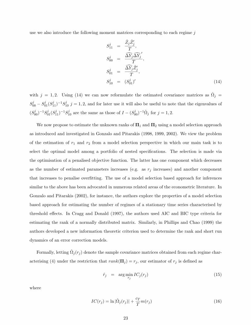
use we also introduce the following moment matrices corresponding to each regime j

Sj11 =

ZjZ′j

T,

Sj00 =

∆Yj∆Yj′

T,

Sj01 =

∆YjZ′j

T,

Sj10 = (Sj

01)′ (14)

with j = 1, 2. Using (14) we can now reformulate the estimated covariance matrices as Ωj =

Sj00 − Sj

01(Sj11)

−1Sj10 j = 1, 2, and for later use it will also be useful to note that the eigenvalues of

(Sj00)

−1Sj01(S

j11)

−1Sj10 are the same as those of I − (Sj

00)−1Ωj for j = 1, 2.

We now propose to estimate the unknown ranks of Π1 and Π2 using a model selection approach

as introduced and investigated in Gonzalo and Pitarakis (1998, 1999, 2002). We view the problem

of the estimation of r1 and r2 from a model selection perspective in which our main task is to

select the optimal model among a portfolio of nested specifications. The selection is made via

the optimisation of a penalised objective function. The latter has one component which decreases

as the number of estimated parameters increases (e.g. as rj increases) and another component

that increases to penalise overfitting. The use of a model selection based approach for inferences

similar to the above has been advocated in numerous related areas of the econometric literature. In

Gonzalo and Pitarakis (2002), for instance, the authors explore the properties of a model selection

based approach for estimating the number of regimes of a stationary time series characterised by

threshold effects. In Cragg and Donald (1997), the authors used AIC and BIC type criteria for

estimating the rank of a normally distributed matrix. Similarly, in Phillips and Chao (1999) the

authors developed a new information theoretic criterion used to determine the rank and short run

dynamics of an error correction models.

Formally, letting Ωj(rj) denote the sample covariance matrices obtained from each regime char-

acterising (4) under the restriction that rank(Πj) = rj , our estimator of rj is defined as

rj = arg minrj

ICj(rj) (15)

where

IC(rj) = ln |Ωj(rj)|+ cT

Tm(rj) (16)

23

with m(rj) denoting the number of estimated parameters (here m(rj) = 2prj − r2j ) and cT a

deterministic penalty term. Next, using the fact that

ln |Ωj(rj)| = ln |Sj00|+

rj∑

i=1

(1− λji ) (17)

and noting that Sj00 is independent of the magnitude of rj , we can instead focus on the optimisation

of the following modified criterion

IC(rj) =rj∑

i=1

ln(1− λji ) +

cT

T(2prj − r2

j ). (18)

A clear advantage of using (18) stems from the simplicity of its empirical implementation,

requiring solely the availability of the eigenvalues of I− (Sj00)

−1Ωj for j = 1, 2. It is also interesting

to observe the close similarity between conducting inferences using (18) and, for instance, a formal

likelihood ratio based testing procedure. Focusing on the estimation of r1 for instance our model

selection based approach involves selecting r1 = 0 as the optimal choice if IC(r1 = 0) < IC(r1 = 1)

and r1 = 1 if IC(r1 = 1) < IC(r1 = 0). Equivalently, the model selection based approach points

to r1 = 1 if −T ln(1 − λ11) > 3cT and to r1 = 0 otherwise under a bivariate setting. This is

equivalent to the formulation of a likelihood ratio statistic for testing the null H0 : r1 = 0 against

H1 : r1 = 1, except that here the decision rule is dictated by the magnitude of the penalty term and

the number of estimated parameters. A formal distribution theory for an LR test based approach

for the determination of r1 and r2 a la Johansen can be found in Gonzalo and Pitarakis (2005a).

We next summarise the asymptotic properties of the model selection approach in the following

proposition.

Proposition 6 Letting r0j denote the true rank of Πj for j = 1, 2 and rj defined as in (15), with

cT such that (i) cT →∞ and (ii) cT /T → 0 as T →∞, we have rjp→ r0

j .

The above proposition establishes the weak consistency of the rank estimators obtained through the

model selection based approach. A possible candidate for the choice of the penalty term satisfying

both (i) and (ii) is ct = lnT corresponding to the well known BIC type criterion. It is clear,

however, that other functionals of the sample size may be equally valid (e.g. cT = 2 ln lnT ) making

it difficult to argue in favour of a universally optimal criterion.

Having established the limiting properties of our rank estimators we next concentrate on their

finite and large sample performance across a wide range of possible model configurations. Following

24

Gonzalo and Pitarakis (2002) we implement our experiments using cT = lnT as the penalty term

in (18).

We initially consider the DGP given in (2) under example 1. We have a bivariate system that

is I(1) with a single cointegrating vector (1,−β). We set β = 2 and consider (ρ1, ρ2) = (0,−0.4) so

that the system is characterised by a true rank configuration given by (r1, r2) = (0, 1). In a second

set of experiments we set (ρ1, ρ2) = (−0.2,−0.6) so that this second system has (r1, r2) = (1, 1). Our

results are summarised in Table 5 below, which presents the decision frequencies for each possible

magnitude of rj . Throughout all our experiments qt is assumed to follow the AR(1) process given

by qt = 0.5qt−1 + εt with εt = iid(0, 1) and the true threshold parameter is set at γ0 = 0. As in our

earlier experiments the delay parameter is set at d = 1 throughout.

Table 5: Decision Frequencies in an I(1) System

r1 = 0 r1 = 1 r1 = 2 r2 = 0 r2 = 1 r2 = 2

(r01 = 0, r0

2 = 1), β = 2, (ρ1, ρ2) = (0.0,−0.4)

T = 200 85.26 14.74 0.00 0.00 100.00 0.00

T = 400 93.42 6.58 0.00 0.00 100.00 0.00

T = 1000 100.00 0.00 0.00 0.00 100.00 0.00

(r01 = 1, r0

2 = 1), β = 2, (ρ1, ρ2) = (−0.2,−0.6)

T = 200 34.76 65.24 0.00 0.02 99.98 0.00

T = 400 10.16 89.84 0.00 0.00 100.00 0.00

T = 1000 0.00 100.00 0.00 0.00 100.00 0.00

(r01 = 1, r0

2 = 0), β = 2, (ρ1, ρ2) = (−0.4, 0.0)

T = 200 0.02 99.98 0.00 84.76 15.24 0.00

T = 400 0.00 100.00 0.00 93.50 0.00 0.00

T = 1000 0.00 100.00 0.00 100.00 0.00 0.00

From the decision frequencies presented in Table 5 above it is clear that the proposed model se-

lection procedure performs remarkably well across the three alternative specifications. As expected

from our result in Proposition 6 it is pointing to the true magnitude of each rank 100% of the

times under T=1000, while maintaining very high correct decision frequencies even under T=200.

Under the specification in (2), for instance, with (r01, r

02) = (0, 1), the procedure picked r1 = 0 about

85% of the times and r2 = 1 100% of the times under T=200, with the correct decision frequency

increasing to about (93%, 100%) under T=400.

25

To provide further empirical support for our proposed approach we next consider a set of

threshold DGPs that restrict Yt to be covariance stationary. For this purpose we have focused on

the specification given in (3) under example 2 and considered two alternative rank configurations.

First, imposing (ρ11, ρ12) = (0, 0) and (ρ21, ρ22) = (−0.2,−0.4) we have a covariance stationary

system with (r1, r2) = (0, 2). Second, setting (ρ11, ρ12, ρ21, ρ22) = (−0.4, 0.0, 0.0,−0.2) we have

another covariance stationary system this time with (r1, r2) = (1, 1). All simulation results are

presented in Table 6 below.

Table 6: Decision Frequencies in a Stationary System

r1 = 0 r1 = 1 r1 = 2 r2 = 0 r2 = 1 r2 = 2

(r01 = 0, r0

2 = 2), (ρ11, ρ12, ρ21, ρ22) = (0.0, 0.0,−0.2,−0.4)

T = 200 88.36 10.24 1.40 0.00 0.00 100.00

T = 400 94.16 5.32 0.52 0.00 0.00 100.00

T = 1000 100.00 0.00 0.00 0.00 0.00 100.00

(r01 = 1, r0

2 = 1), (ρ11, ρ12, ρ21, ρ22) = (−0.4, 0.0, 0.0,−0.2)

T = 200 0.00 86.90 13.10 0.56 86.94 12.50

T = 400 0.00 90.38 0.00 0.00 91.00 9.00

T = 1000 0.00 92.64 7.36 0.00 92.96 7.04

From the empirical decision frequencies presented above it is again the case that the various es-

timators of r1 and r2 point to their true counterparts as T is allowed to increase. Although the

accuracy of the estimators is somehow determined by the DGP specific parameters it is also clear

that under both experiments the frequency of pointing to the true rank is high, reaching levels

ranging between 90 and 100% accuracy.

5 A Nonlinear Permanent and Transitory Decomposition

Having established the threshold cointegration properties of Yt, we next investigate how this vector

process of interest can be decomposed into a permanent and transitory component following the

methodology developed in Gonzalo and Granger (1995).

Recall that in the linear case with Yt following a VECM of the form ∆Yt = αβ′Yt + ut we are

26

interested in decomposing the p-dimensional vector Yt into two sets of components as

Yt = A1ft + Yt (19)

where A1 is the p× (p− r) loading matrix, ft the (p− r)× 1 common I(1) factors and Yt is the I(0)

component. The above decomposition of Yt is such that the factors ft are linear combinations of

Yt and A1ft and Yt form a Permanent-Transitory decomposition (see Gonzalo and Granger (1995)

for the detailed definitions of each component).

As shown in Gonzalo and Granger (1995), the above two conditions are sufficient to identify

the permanent and transitory components. Formally we can write

Yt = A1ft + A2zt (20)

with ft = α⊥Yt, zt = β′Yt and A1 = β⊥(α′⊥β⊥)−1, A2 = α(β′α)−1. Note that α′⊥α = β′⊥β = 0.

Now, let us consider the following VECM with threshold effects

∆Yt = α1β′Yt−1I(qt−d ≤ γ) + α2β

′Yt−1I(qt−d > γ) + ut.

Following the same reasoning as in Gonzalo and Granger (1995) it is now straightforward to establish

the following Threshold Permanent-Transitory decomposition for Yt

Yt = A1f1tI(qt−d ≤ γ) + A2f2tI(qt−d > γ) + (A3I(qt−d ≤ γ) + A4I(qt−d > γ)zt (21)

where f1t = α′1⊥Yt, f2t = α2⊥Yt and zt = β′Yt. The corresponding loading matrices are then

given by A1 = β⊥(α′1⊥β⊥)−1, A2 = β⊥(α′2⊥β⊥)−1 and similarly A3 = α1(β′α1)−1 and A4 =

α2(β′α2)−1. Given our estimator of the threshold parameter γ defined in (9) together with the

corresponding sample moment matrices introduced in (14), the practical implementation of the

above Threshold Permanent and Transitory decomposition becomes straightforward (see Gonzalo

and Pitarakis (2005b)) and is obtained following the same approach as in Gonzalo and Granger

(1995).

Despite the representational complications that would arise if we were to also allow the coin-

tegrating vector β to be characterised by the presence of threshold effects as say βt = β1I(qt−d ≤γ) + β2I(qt−d > γ) (see our discussion in section 4.2) the above threshold based decomposi-

tion would translate naturally to such a framework by reformulating it as Yt = A1f1tI(qt−d ≤

27

γ)+A2f2tI(qt−d > γ)+A3z1tI(qt−d ≤ γ)+A4z2tI(qt−d > γ), with z1t = β′1Yt, z2t = β′2Yt. The cor-

responding loading matrices would then be given by A1 = β1⊥(α′1⊥β1⊥)−1, A2 = β2⊥(α′2⊥β2⊥)−1,

A3 = α1(β′1α1)−1 and A4 = α2(β′2α2)−1.

6 Conclusions

This chapter has focused on the issue of introducing and testing for threshold type nonlinear

behaviour into the conventional multivariate error correction model. The threshold nonlinearities

we considered were driven by a stationary and external random variable triggering the regime

switches. Within this context we obtained the limiting properties of a Wald type test statistic for

testing for the presence of such threshold effects characterising the long run impact matrix of the

VECM. An interesting property of the proposed test is its robustness to the presence or absence

of unit roots in the system, displaying the same limiting null distribution under a wide range of

stochastic properties of the system.

We subsequently proceeded with the interpretation and further analysis of the system following

a rejection of the null hypothesis of linearity. We showed that cointegration as traditionally defined

was compatible with such an error correction type specification only if the nonlinearities are present

in the adjustment process rather than the long run equilibrium itself. We then introduced a model

selection based approach designed to gain further insight into the stochastic properties of the system

through the determination of the rank structure of the long run impact matrices characterising each

regime. This then allowed us to extend the permanent and transitory decomposition of Gonzalo

and Granger (1995) into a nonlinear permanent and transitory decomposition.

Much remains to be done in the area of nonlinear multivariate specifications such as the

VAR/VECMs considered here. In this paper for instance we restricted our analysis to models

with no deterministic trends. Similarly our results also ignored the possibility of having such com-

ponents together with the lagged dependent variables and cointegrating vectors display threshold

switching behaviour. Extensions along these lines together with a formal representation theory for

such models are topics currently being investigated by the authors.

28

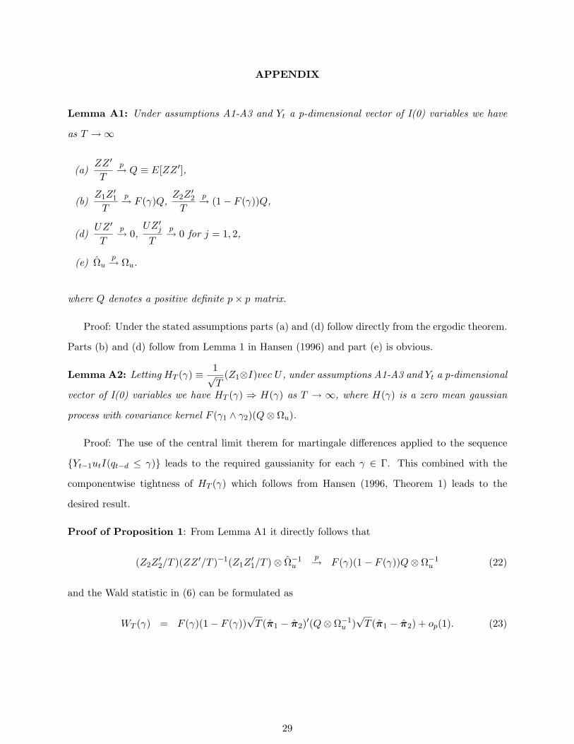
APPENDIX

Lemma A1: Under assumptions A1-A3 and Yt a p-dimensional vector of I(0) variables we have

as T →∞

(a)ZZ ′

T

p→ Q ≡ E[ZZ ′],

(b)Z1Z

′1

T

p→ F (γ)Q,Z2Z

′2

T

p→ (1− F (γ))Q,

(d)UZ ′

T

p→ 0,UZ ′jT

p→ 0 for j = 1, 2,

(e) Ωup→ Ωu.

where Q denotes a positive definite p× p matrix.

Proof: Under the stated assumptions parts (a) and (d) follow directly from the ergodic theorem.

Parts (b) and (d) follow from Lemma 1 in Hansen (1996) and part (e) is obvious.

Lemma A2: Letting HT (γ) ≡ 1√T

(Z1⊗I)vec U , under assumptions A1-A3 and Yt a p-dimensional

vector of I(0) variables we have HT (γ) ⇒ H(γ) as T → ∞, where H(γ) is a zero mean gaussian

process with covariance kernel F (γ1 ∧ γ2)(Q⊗ Ωu).

Proof: The use of the central limit therem for martingale differences applied to the sequence

Yt−1utI(qt−d ≤ γ) leads to the required gaussianity for each γ ∈ Γ. This combined with the

componentwise tightness of HT (γ) which follows from Hansen (1996, Theorem 1) leads to the

desired result.

Proof of Proposition 1: From Lemma A1 it directly follows that

(Z2Z′2/T )(ZZ ′/T )−1(Z1Z

′1/T )⊗ Ω−1

up→ F (γ)(1− F (γ))Q⊗ Ω−1

u (22)

and the Wald statistic in (6) can be formulated as

WT (γ) = F (γ)(1− F (γ))√

T (π1 − π2)′(Q⊗ Ω−1u )

√T (π1 − π2) + op(1). (23)

29

Standard least squares algebra together with Lemma A1 also imply

√T (π1 − π) =

√T [(Z1Z

′1)−1Z1 ⊗ Ip]vec U

=

[(Z1Z

′1

T

)−1

⊗ Ip

]1√T

(Z1 ⊗ Ip)vec U

=1

F (γ)(Q−1 ⊗ Ip)

1√T

(Z1 ⊗ Ip)vec U + op(1) (24)

and

√T (π2 − π) =

[(Z2Z

′2

T

)−1

⊗ Ip

]1√T

(Z2 ⊗ Ip)vec U

=1

(1− F (γ))(Q−1 ⊗ Ip)

1√T

(Z2 ⊗ Ip)vec U + op(1). (25)

Combining (24) and (25) above and using the fact that Z2 = Z − Z1 we have

√T (π1 − π2) =

(Q−1 ⊗ I)F (γ)(1− F (γ))

[1√T

(Z1 ⊗ I)vec U − F (γ)1√T

(Z ⊗ I)vec U

]+ op(1).(26)

We can now write the Wald statistic as

WT (γ) =[

1√T

(Z1 ⊗ I)vecU − F (γ)1√T

(Z ⊗ I)vecU

]′V (γ)−1

[1√T

(Z1 ⊗ I)vecU − F (γ)1√T

(Z ⊗ I)vecU

]+ op(1). (27)

where V (γ) = F (γ)(1−F (γ))(Q⊗Ωu). Next letting GT (γ) ≡ [(Z1⊗I)vecU−F (γ)(Z⊗I)vecU ]/√

T ,

Lemmas A1-A2 together with the fact that 1√T

(Z⊗ I)vec Ud→ N(0, Q⊗Ωu) which follows directly

from the CLT imply GT (γ) ⇒ G(γ), where G(γ) is a zero mean gaussian random vector with

covariance E[G(γ1)G(γ2)] = V (γ1 ∧ γ2) ≡ F (γ1 ∧ γ2)(1− F (γ1 ∧ γ2))(Q⊗Ωu). It now follows that

the limiting distribution of the Wald statistic WT (γ) is given by WT (γ) ⇒ G(γ)′V (γ)−1G(γ) and

the final result follows from the continuous mapping theorem.

Lemma A3: Under assumptions A1-A3 and Yt a p-dimensional vector of I(1) variables with

∆Y = U we have as T →∞

(a)ZZ ′

T 2⇒

∫ 1

0W (r)W (r)′dr,

(b)Z1Z

′1

T 2⇒ F (γ)

∫ 1

0W (r)W (r)′dr,

(c)Z2Z

′2

T 2⇒ (1− F (γ))

∫ 1

0W (r)W (r)′dr

30

where W (r)′ = (W1(r), . . . , Wp(r)) is a p-dimensional standard Brownian Motion.

Proof: Part (a) follows directly from Phillips and Durlauf (1986). For part (b) we first write

Z1Z′1

T 2= F (γ)

ZZ ′

T 2+

W1W′1

T 2(28)

where W1W′1 stacks the elements of the form Yt−1Y

′t−1(I(qt−d ≤ γ) − F (γ)). It now suffices to

show that W1W ′1

T 2 = op(1). We let St =∑t

i=1(I(qt−1 ≤ γ) − F (γ)) and with no loss of generality

set d = 1 and take zero initial conditions. Using summation by parts we can write∑T

t=1(I(qt−1 ≤γ)−F (γ))Yt−1Y

′t−1 = ST−1YT Y ′

T −∑T−1

t=1 St(Yt+1Y′t+1−YtY

′t ). Next using the fact that Yt+1Y

′t+1 =

YtY′t + Ytu

′t+1 + ut+1Y

′t + ut+1u

′t+1 we also have

1T 2

W1W′1 =

ST−1

T

YT Y ′T

T− 1

T 2

T−1∑

t=1

Ytu′t+1St − 1

T 2

T−1∑

t=1

ut+1Y′t St −

1T 2

T−1∑

t=1

(ut+1u′t+1 − Ωu)St − 1

T 2Ωu

T−1∑

t=1

St. (29)

Under the maintained assumptions the ergodic theorem ensures that ST−1/Tp→ 0. Since YT Y ′

T /T is

stochastically bounded it thus follows that the first term in the right hand side of (29) is op(1). Next,

we consider the components yitujt+1St. We have E[yitujt+1St] = 0 and it is also straightforward to

establish that

limT→∞

E

[1T 2

T−1∑

t=1

yit−1ujtSt

]2

= 0

and both the second and third terms in the right hand side of (29) are also op(1). Proceeding

similarly, the third and fourth components can also be seen to be op(1) and the final result follows

from (a). Part (c) can be shown to hold in exactly the same manner as part (b).

Lemma A4: Under assumptions A1-A3 and Yt a p-dimensional vector of I(1) variables with

∆Y = U we have as T →∞

(a)1T

(Z ⊗ Ip)vec U ⇒ vec

[∫ 1

0dW (r)W (r)′

],

(b)1T

(Z1 ⊗ Ip)vec U ⇒ vec

[∫ 1

0dW (r, F (γ))W (r)′

]

Proof: Part (a) follows directly from Phillips and Durlauf (1986). For part (b), the result

follows from LT (γ) ≡ 1√T

∑[Tr]t=1 utI(qt−1 ≤ γ) ⇒ W (r, F (γ)) where W (r, F (γ)) denotes a standard

31

Brownian Sheet (see Theorem 1 in Diebolt, Laib and Wandji (1997)) and Theorem 2 in Caner and

Hansen (2001).

Proof of Proposition 2 We assume that the underlying null model is a pure unit root process as

∆Y = U . Within the present I(1) framework we consider the following normalisation of the Wald

statistic

T (π1 − π2)′[(

Z2Z′2

T 2

)(ZZ ′

T 2

)−1 (Z1Z

′1

T 2

)⊗ Ω−1

u

]T (π1 − π2).

and with no loss of generality in what follows we will impose Ωu = Ip. Next, from Lemma A3 it

follows that[(

Z2Z′2

T 2

)(ZZ ′

T 2

)−1 (Z1Z

′1

T 2

)⊗ Ω−1

u

]⇒ F (γ)(1− F (γ))

∫ 1

0W (r)W (r)′dr ⊗ Ip. (30)

and we formulate the test statistic of interest as

WT (γ) = F (γ)(1− F (γ))T (π1 − π2)′[∫ 1

0W (r)W (r)′dr ⊗ Ip

]T (π1 − π2) + op(1).

We next focus on the large sample behaviour of T (π1−π2) when the true DGP is given by ∆Y = U .

We have

T π1 =

[(Z1Z

′1

T 2

)−1

⊗ Ip

]1T

(Z1 ⊗ Ip)vec U

=1

F (γ)

[(∫ 1

0W (r)W (r)′dr

)−1

⊗ Ip

]1T

(Z1 ⊗ Ip)vec U + op(1). (31)

Proceeding similarly for π2 and rearranging as above we have

T (π1 − π2) =1

F (γ)(1− F (γ))

[(∫ 1

0WW ′

)−1

⊗ Ip

][1T

(Z1 ⊗ Ip)vec U − F (γ)1T

(Z ⊗ Ip)vec U

]

Next, using Lemma A4 it follows that

1T

(Z1 ⊗ I)vecU − F (γ)1T

(Z ⊗ I)vecU ⇒ vec

[∫ 1

0dW (r, F (γ))W (r)′

]− F (γ)vec

[∫ 1

0dW (r, 1)W (r)′

]

= vec

[∫ 1

0[dW (r, F (γ))− F (γ)dW (r, 1)]W (r)′

]

= vec

[∫ 1

0dK(r, F (γ))W (r)′

](32)

32

where we let K(r, F (γ)) = W (r, F (γ)) − F (γ)W (r, 1). Using the above in the expression of the

Wald test statistic and rearranging we obtain the required result. The case for a cointegrated

system follows along the same lines.

Proof of Proposition 3 From U(γ) = ∆Y − Π1Z1 − Π2Z2 + U we can write

U(γ)U(γ)′ = (∆Y − Π1Z1 − Π2Z2)(∆Y ′ − Z ′1Π′1 − Z ′2Π

′2)

= ∆Y ∆Y ′ −∆Y Z ′1(Z1Z′1)−1Z1∆Y ′ −∆Y Z ′2(Z2Z

′2)−1Z2∆Y ′ (33)

where we made use of the fact that ZiZ′j = 0 ∀i 6= j and i, j = 1, 2. Next, letting γ0 denote the

true threshold parameter we write the model evaluated at γ0 as ∆Y = Π1Z01 + Π2Z

02 + U where

Z01 = (y0I(q0−d ≤ γ0), . . . , yT−1I(qT−d ≤ γ0)) and Z0

2 = Z − Z01 with Z0

1Z02′ = 0. Inserting into

(33) and rearranging gives

U(γ)U(γ)′ = Π1Z01Z0

1Π′1 + Π2Z

02Z0

2Π′2 + 2Π1Z

01U ′ + 2Π2Z

02U ′ + UU ′ −Π1Z

01M1Z

01′Π′

1 −Π2Z

02M1Z

02′Π′

1 − 2Π1Z01M1Z

02′Π′

2 − 2Π1Z01M1U

′ − 2Π2Z02M1U

′ − UM1U′ −Π1Z

01M2Z

01′Π′

1 −Π2Z

02M2Z

02′Π′

2 − 2Π1Z01M2Z

02′Π′

2 − 2Π1Z01M2U

′ − 2Π2Z02M2U

′ − UM2U′

where M1 = Z ′1(Z1Z′1)−1Z1 and M2 = Z ′2(Z2Z

′2)−1Z2. We next evaluate the limiting behaviour of

the above quantity for γ < γ0, γ = γ0 and γ > γ0. Applying appropriate normalisations we obtain

the following uniform convergence in probability result over γ ∈ Γ for the case γ < γ0

U(γ)U(γ)′

T

p→ (Π1 −Π2)[(G(γ0)−G(γ))(G−G(γ))−1(G−G(γ0))](Π1 −Π2)′ + Ωu

≡ (F (γ0)− F (γ))(1− F (γ0))1− F (γ)

(Π1 −Π2)Q(Π1 −Π2)′ + Ωu. (34)

Proceeding similarly for the case γ > γ0 we have

U(γ)U(γ)′

T

p→ (Π1 −Π2)[G(γ0)G(γ)−1(G(γ)−G(γ0))](Π1 −Π2)′ + Ωu

≡ F (γ0)(F (γ)− F (γ0))F (γ)

(Π1 −Π2)Q(Π1 −Π2)′ + Ωu.

Finally with

U(γ0)U(γ0)′

T

p→ Ωu

we have that the objective function converges uniformly in probability to a nonstochastic limit that

is uniquely minimised at γ = γ0 and the required result follows from Theorem 2.1 in Newey and

McFadden (1994).

33

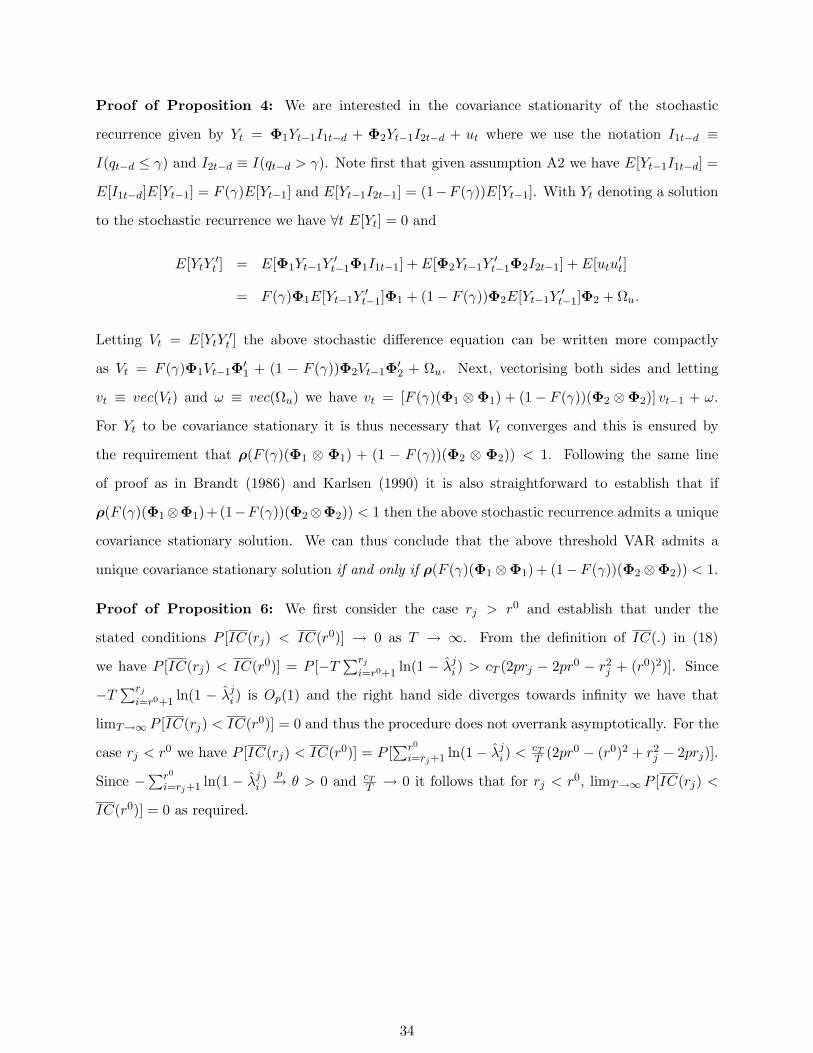
Proof of Proposition 4: We are interested in the covariance stationarity of the stochastic

recurrence given by Yt = Φ1Yt−1I1t−d + Φ2Yt−1I2t−d + ut where we use the notation I1t−d ≡I(qt−d ≤ γ) and I2t−d ≡ I(qt−d > γ). Note first that given assumption A2 we have E[Yt−1I1t−d] =

E[I1t−d]E[Yt−1] = F (γ)E[Yt−1] and E[Yt−1I2t−1] = (1−F (γ))E[Yt−1]. With Yt denoting a solution

to the stochastic recurrence we have ∀t E[Yt] = 0 and

E[YtY′t ] = E[Φ1Yt−1Y

′t−1Φ1I1t−1] + E[Φ2Yt−1Y

′t−1Φ2I2t−1] + E[utu

′t]

= F (γ)Φ1E[Yt−1Y′t−1]Φ1 + (1− F (γ))Φ2E[Yt−1Y

′t−1]Φ2 + Ωu.

Letting Vt = E[YtY′t ] the above stochastic difference equation can be written more compactly

as Vt = F (γ)Φ1Vt−1Φ′1 + (1 − F (γ))Φ2Vt−1Φ′

2 + Ωu. Next, vectorising both sides and letting

vt ≡ vec(Vt) and ω ≡ vec(Ωu) we have vt = [F (γ)(Φ1 ⊗Φ1) + (1− F (γ))(Φ2 ⊗Φ2)] vt−1 + ω.

For Yt to be covariance stationary it is thus necessary that Vt converges and this is ensured by

the requirement that ρ(F (γ)(Φ1 ⊗ Φ1) + (1 − F (γ))(Φ2 ⊗ Φ2)) < 1. Following the same line

of proof as in Brandt (1986) and Karlsen (1990) it is also straightforward to establish that if

ρ(F (γ)(Φ1⊗Φ1)+(1−F (γ))(Φ2⊗Φ2)) < 1 then the above stochastic recurrence admits a unique

covariance stationary solution. We can thus conclude that the above threshold VAR admits a

unique covariance stationary solution if and only if ρ(F (γ)(Φ1 ⊗Φ1) + (1− F (γ))(Φ2 ⊗Φ2)) < 1.

Proof of Proposition 6: We first consider the case rj > r0 and establish that under the

stated conditions P [IC(rj) < IC(r0)] → 0 as T → ∞. From the definition of IC(.) in (18)

we have P [IC(rj) < IC(r0)] = P [−T∑rj

i=r0+1ln(1 − λj

i ) > cT (2prj − 2pr0 − r2j + (r0)2)]. Since

−T∑rj

i=r0+1ln(1 − λj

i ) is Op(1) and the right hand side diverges towards infinity we have that

limT→∞ P [IC(rj) < IC(r0)] = 0 and thus the procedure does not overrank asymptotically. For the

case rj < r0 we have P [IC(rj) < IC(r0)] = P [∑r0

i=rj+1 ln(1− λji ) < cT

T (2pr0 − (r0)2 + r2j − 2prj)].

Since −∑r0

i=rj+1 ln(1 − λji )

p→ θ > 0 and cTT → 0 it follows that for rj < r0, limT→∞ P [IC(rj) <

IC(r0)] = 0 as required.

34

REFERENCES

Andrews, D. W. K., 1993. Tests for Parameter Stability and Structural Change with Unknown

Change Point, Econometrica, 61, 821-856.

Arai, Y., 2004. Testing for linearity in regressions with I(1) processes, CIRJE Discussion Paper

No. F-303, University of Tokyo.

Balke, N., Fomby, T., 1997. Threshold Cointegration, International Economic Review, 38,

627-645.

Baum, C. F., Barkoulas, J. T, Caglayan, M., 2001. Nonlinear adjustment to purchasing power

parity in the post Bretton Woods era, Journal of International Money and Finance, 20, 379-399.

Beaudry, P., Koop, G., 1993. Do recessions permanently change output? Journal of Monetary

Economics, 31, 149-164.

Bec, F., Ben-Salem, M., Carrasco, M., 2001. Tests for unit-root versus Threshold specification

with an application to the PPP, Journal of Business and Economic Statistics, forthcoming.

Bec, F., Rahbek, A., 2004. Vector equilibrium correction models with nonlinear discontinuous

adjustments, Econometrics Journal, 7, 1-24.

Borenstein, S. A., Cameron, A. C., Gilbert, R., 1997. Do gasoline prices respond asymmetrically

to crude oil prices? Quarterly Journal of Economics, 112, 305-339.

Brandt, A., 1986. The stochastic equation Yn+1 = AnYn + Bn with stationary coefficients,

Advances in Applied Probability, 18, 211-220.

Caner, M., Hansen, B. E., 2001. Threshold autoregression with a unit root. Econometrica, 69,

1555-1596.

Chan, K. S., 1990. Testing for threshold autoregression, Annals of Statistics, 18, 1886-1894.

Chan, K. S., 1993. Consistency and limiting distribution of the least squares estimator of a

threshold autoregressive model, Annals of Statistics, 21, 520-533.

Cragg, J. G., Donald, S. G., 1997. Inferring the rank of a matrix, Journal of Econometrics, 76,

223-250.

35

Diebolt, J., Laib, N., Ngatchou-Wandji, J., 1997. Limiting distributions of weighted pro-

cesses of residuals. Application to parametric nonlinear autoregressive models, Comptes Rendus

de l’Academie des Sciences de Paris, Series 1, 325, 535-540.

Durlauf, S. N., Johnson, P. A., 1995. Multiple regimes and cross-country growth behaviour,

Journal of Applied Econometrics, 10, 365-384.

Enders, W., Falk, B., 1998. Threshold-autoregressive, median-unbiased, and cointegration tests

of purchasing power parity, International Journal of Forecasting, 14, 171-186.

Enders, W., Granger, C. W. J., 1998. Unit-root tests and asymmetric adjustment with an

example using the term structure of interest rates, Journal of Business and Economic Statistics,

16, 304-311.

Enders, W., Siklos, P. L., 2001. Cointegration and Threshold Adjustment. Journal of Business

and Economic Statistics, 19, 166-176.

Engle, R. F., Granger, C. W. J., 1987. Co-Integration and Error Correction: representation,

estimation and testing, Econometrica, 55, 251-276.

Gonzalez, M., Gonzalo, J., 1997. Threshold Unit Root Processes. Unpublished manuscript,

Department of Statistics and Econometrics, Universidad Carlos III de Madrid.

Gonzalo, J., Granger, C. W. J., 1995. Estimation of Common Long-Memory Components in

Cointegrated Systems, Journal of Business and Economic Statistics, 13, 27-35.

Gonzalo, J., Montesinos, R., 2000. Threshold Stochastic Unit Root Models, Unpublished

manuscript, Department of Statistics and Econometrics, Universidad Carlos III de Madrid.

Gonzalo, J., Pitarakis, J-Y., 1998. Specification via model selection in vector error correction

models, Economics Letters, 60, 321-328.

Gonzalo, J., Pitarakis, J-Y., 1999. Dimensionality effect in cointegration analysis. In: Engle,

R. F., White, H. (Eds.). Cointegration, Causality and Forecasting: A Festschrift in Honour of C.

W. J. Granger. Oxford University Press, Oxford, pp. 212-229.

Gonzalo, J., Pitarakis, J-Y., 2002. Estimation and Model Selection Based Inference in Single

and Multiple Threshold Models, Journal of Econometrics, 110, 319-352.

36

Gonzalo, J., Pitarakis, J-Y., 2005a. Threshold Nonlinearities in Cointegrated Systems, Unpub-

lished Manuscript.

Gonzalo, J., Pitarakis, J-Y., 2005b. Estimation of Common Long-Memory Components in

Threshold Cointegrated Systems, Unpublished Manuscript.

Granger, C. W. J., Inoue, T., Morin, N., 1997. Nonlinear Stochastic Trends, Journal of Econo-

metrics, 81, 65-92.

Hansen, B. E., 1996. Inference when a nuisance parameter is not identified under the null

hypothesis, Econometrica, 64, 413-430.

Hansen, B. E., 1997. Approximate asymptotic p-values for structural change tests, Journal of

Business and Economic Statistics, 15, 60-67.

Hansen, B. E., 1999a. Testing for linearity. Journal of Economic Surveys, 13, 551-576.

Hansen, B. E., 1999b. Threshold effect in nondynamic panels: estimation, testing and inference,

Journal of Econometrcs, 93, 345-368.

Hansen, B. E., Seo, B., 2002. Testing for two-regime threshold cointegration in vector error

correction models, Journal of Econometrics, 110, 293-318.

Hong, S., 2003. Testing Linearity in Cointegrating Relations: Application to PPP, mimeo, Yale

University, Unpublished Manuscript.

Johansen, S., 1988. Statistical analysis of cointegrating vectors, Journal of Economic Dynamics

and Control, 12, 231-254.

Johansen S., 1991. Estimation and hypothesis testing of cointegrating vectors in Gaussian

vector autoregressive models, Econometrica, 59, 1551-1580.

Johansen, S., 1995. Likelihood based inference in cointegrated vector autoregressive models,

Oxford University Press.

Karlsen, H. A., 1990. Existence of moments in a stationary stochastic difference equation,

Advances in Applied Probability, 22, 129-146.

Koop, G., Potter, S. M., 1999. Dynamic asymmetries in US unemployment, Journal of Business

and Economic Statistics, 17, 298-312.

37

Lo, M. C., Zivot, E., 2001. Threshold cointegration and nonlinear adjustment to the law of one

price, Macroeconomic Dynamics 5, 533576.

Michael, P., Nobay, A. R., Peel, D. A., 1997. Transaction costs and nonlinear adjustment in

real exchange rates: an empirical investigation, Journal of Political Economy 105, 862879.

Newey, W. K., McFadden, D. L., 1994. Large sample estimation and hypothesis testing, In:

Engle, R. F., McFadden, D. L. (Eds.). Handbook of Econometrics, Vol. 4, Elsevier, New York, pp.

2113-2245.

Obstfeld, M., Taylor, A. M., 1997. Nonlinear aspects of goods-market arbitrage and adjustment:

Heckschers commodity points revisited, Journal of the Japanese and International Economies 11,

441-479.

O’Connell, P. G. J., Wei, S., 1997. The bigger they are the harder they fall: how price differences

across U.S. cities are arbitraged. Journal of International Economics, 56, 21-53.

Peltzman, S., 2000. Prices rise faster than they fall, Journal of Political Economy, 108, 466-502.

Phillips, P. C. B., Chao, J. C., 1999. Model selection in partially nonstationary vector autore-

gressive processes with reduced rank structure, Journal of Econometrics, 91,

Phillips, P. C. B., Durlauf, S., 1986. Multiple Time Series Regression with Integrated Processes,

Review of Economic Studies, 53, 473-495.

Pippenger, M. K., Goering, G. E., 1993. A Note on the Empirical Power of Unit Root Tests

under Threshold Processes, Oxford Bulletin of Economics and Statistics, 55, 473-481.

Potter, S. M., 1995. A nonlinear approach to US GNP. Journal of Applied Econometrics, 2,

109-125.

Saikkonen, P., Choi, I., 2004. Cointegrating Smooth Transition Regressions, Econometric The-

ory, 20, 301-340.

Seo, M., 2004. Bootstrap testing for the presence of threshold cointegration in a threshold

vector error correction model, Unpublished Manuscript, Department of Economics, University of

Wisconsin-Madison.

Tong, H., Lim, K. S., 1980. Threshold autoregression, limit cycles and cyclical data, Journal of

38

the Royal Statistical Society, Series B, 4, 245-292.

Tong, H., 1983. Threshold models in non-linear time series analysis. Lecture Notes in Statistics,

Vol. 21. Springer, Berlin.

Tong, H., 1990. Non-Linear Time Series: A Dynamical System Approach. Oxford University

Press, Oxford.

Tsay, R. S., 1989. Testing and modeling threshold autoregressive processes. Journal of the

American Statistical Association, 84, 231-240.

Tsay, R. S., 1998. Testing and modeling multivariate threshold models. Journal of the American

Statistical Association, 93, 1188-1202.

Wohar, M. E., Balke, N. S., 1998. Nonlinear dynamics and covered interest rate parity, Empir-

ical Economics, 23, 535-559.

39