Graduate Theses and Dissertations Iowa State University Capstones, Theses andDissertations

2017

Threshold-based synchrophasor monitoring ofmultiple outages on a detailed WECC system usingarea angleVikram Kumar Reddy ChilukaIowa State University

Follow this and additional works at: https://lib.dr.iastate.edu/etd

Part of the Electrical and Electronics Commons

This Thesis is brought to you for free and open access by the Iowa State University Capstones, Theses and Dissertations at Iowa State University DigitalRepository. It has been accepted for inclusion in Graduate Theses and Dissertations by an authorized administrator of Iowa State University DigitalRepository. For more information, please contact digirep@iastate.edu.

Recommended CitationChiluka, Vikram Kumar Reddy, "Threshold-based synchrophasor monitoring of multiple outages on a detailed WECC system usingarea angle" (2017). Graduate Theses and Dissertations. 16329.https://lib.dr.iastate.edu/etd/16329

brought to you by COREView metadata, citation and similar papers at core.ac.uk

provided by Digital Repository @ Iowa State University

Threshold-based synchrophasor monitoring of multiple outages on a detailed WECC system using area angle

by

Vikram Kumar Reddy Chiluka

A thesis submitted to the graduate faculty

in partial fulfillment of the requirements for the degree of

MASTER OF SCIENCE

Major: Electrical Engineering

Program of Study Committee: Ian Dobson, Major Professor

Venkataramana Ajjarapu Manimaran Govindarasu

The student author, whose presentation of the scholarship herein was approved by the program of study committee, is solely responsible for the content of this thesis. The Graduate

College will ensure this thesis is globally accessible and will not permit alterations after a degree is conferred.

Iowa State University

Ames, Iowa

2018

Copyright © Vikram Kumar Reddy Chiluka, 2018. All rights reserved.

ii

TABLE OF CONTENTS

Page

LIST OF TABLES . . . . . . . . . . . . . . . . . . . . . . . . . . . . . . . . . . . . . . . . . . iv

LIST OF FIGURES . . . . . . . . . . . . . . . . . . . . . . . . . . . . . . . . . . . . . . . . . v

ACKNOWLEDGEMENTS . . . . . . . . . . . . . . . . . . . . . . . . . . . . . . . . . . . . . vii

ABSTRACT . . . . . . . . . . . . . . . . . . . . . . . . . . . . . . . . . . . . . . . . . . . . . viii

CHAPTER 1. INTRODUCTION . . . . . . . . . . . . . . . . . . . . . . . . . . . . . . . . . 1

1.1 Objective . . . . . . . . . . . . . . . . . . . . . . . . . . . . . . . . . . . . . . . . . . 2

1.2 Organization of Thesis . . . . . . . . . . . . . . . . . . . . . . . . . . . . . . . . . . . 3

CHAPTER 2. REVIEW OF AREA ANGLE . . . . . . . . . . . . . . . . . . . . . . . . . . . 4

2.1 Calculation of area angle and power across the area . . . . . . . . . . . . . . . . . . . 4

2.2 Selection of Border Buses . . . . . . . . . . . . . . . . . . . . . . . . . . . . . . . . . 5

2.3 Evaluating the maximum power that can enter an area under single line contingencies 6

2.4 Monitoring multiple outages . . . . . . . . . . . . . . . . . . . . . . . . . . . . . . . . 8

2.4.1 Simple example . . . . . . . . . . . . . . . . . . . . . . . . . . . . . . . . . . . 8

2.4.2 Algorithm . . . . . . . . . . . . . . . . . . . . . . . . . . . . . . . . . . . . . . 10

2.5 Exceptional outages . . . . . . . . . . . . . . . . . . . . . . . . . . . . . . . . . . . . 12

CHAPTER 3. DESCRIPTION OF POWER SYSTEM NETWORK MODEL . . . . . . . . 14

CHAPTER 4. AREAS, AREA ANGLES AND THRESHOLDS . . . . . . . . . . . . . . . . 16

4.1 Idaho Area Simulation . . . . . . . . . . . . . . . . . . . . . . . . . . . . . . . . . . . 16

4.1.1 Outages and the calculation of thresholds for area angle . . . . . . . . . . . . 16

iii

4.2 Southern California Area . . . . . . . . . . . . . . . . . . . . . . . . . . . . . . . . . 19

4.2.1 Outages and area angle thresholds . . . . . . . . . . . . . . . . . . . . . . . . 20

4.3 Robustness to changing stress direction . . . . . . . . . . . . . . . . . . . . . . . . . 22

4.4 Effect of exceptional outages . . . . . . . . . . . . . . . . . . . . . . . . . . . . . . . 24

CHAPTER 5. CONCLUSION . . . . . . . . . . . . . . . . . . . . . . . . . . . . . . . . . . . 26

REFERENCES . . . . . . . . . . . . . . . . . . . . . . . . . . . . . . . . . . . . . . . . . . . . 28

APPENDIX. SYSTEM MODELLING AND COMPUTATION . . . . . . . . . . . . . . . . 30

iv

LIST OF TABLES

Page

Table 2.1 Simple example demonstrating that area angle tracks severity . . . . . . . . 10

Table 2.2 The possibilities of exceptional outages . . . . . . . . . . . . . . . . . . . . . 12

Table 2.3 Exceptional outages in simple network . . . . . . . . . . . . . . . . . . . . . 13

Table 3.1 Difference between the reduced model and detailed model . . . . . . . . . . 14

v

LIST OF FIGURES

Page

Figure 1.2 Border buses for a load area . . . . . . . . . . . . . . . . . . . . . . . . . . . 2

Figure 1.3 Border buses for a transfer path area . . . . . . . . . . . . . . . . . . . . . . 2

Figure 2.1 Area angle representation . . . . . . . . . . . . . . . . . . . . . . . . . . . . 5

Figure 2.2 Simple example on monitoring multiple outages . . . . . . . . . . . . . . . . 9

Figure 2.3 Simple network for illustrating exceptional outages . . . . . . . . . . . . . . 13

Figure 3.1 Angles at the buses plotted on WECC. The black color represents a higher

value and blue color represents a lower value . . . . . . . . . . . . . . . . . . 15

Figure 4.1 Idaho Area - Border Ma buses are colored in red and border Mb buses area

colored in blue. Numbers represent the weights . . . . . . . . . . . . . . . . 17

Figure 4.2 Single line non-exceptional outages for Southern Idaho area. Outages are

ordered so the maximum power increases. . . . . . . . . . . . . . . . . . . . 17

Figure 4.3 Random sample of 1700 double line non-exceptional outages for Southern

Idaho area . . . . . . . . . . . . . . . . . . . . . . . . . . . . . . . . . . . . . 18

Figure 4.4 Random sample of 1396 triple line non-exceptional outages for Southern

Idaho area. . . . . . . . . . . . . . . . . . . . . . . . . . . . . . . . . . . . . . 18

Figure 4.5 Southern California Area . . . . . . . . . . . . . . . . . . . . . . . . . . . . . 19

Figure 4.6 Single line non-exceptional outages for Southern California area. Outages

are ordered so that maximum power increases . . . . . . . . . . . . . . . . . 20

Figure 4.7 Random sample of 512 double line non-exceptional outages for Southern

California area. . . . . . . . . . . . . . . . . . . . . . . . . . . . . . . . . . . 21

vi

Figure 4.8 Random sample of 2020 triple line non-exceptional outages for Southern

California area. . . . . . . . . . . . . . . . . . . . . . . . . . . . . . . . . . . 21

Figure 4.9 Single line outages for reduced BPA network. Pattern of stress used here is

according to weights at the buses . . . . . . . . . . . . . . . . . . . . . . . . 23

Figure 4.10 Single line outages for reduced BPA network. Pattern of stress used here is

proportional to the tie line power flows into the buses. . . . . . . . . . . . . 24

Figure 4.11 All single line outages for Idaho area with exceptional outages colored in red 25

Figure 4.12 Random sample of triple line outages for Idaho area with exceptional outages

colored in red . . . . . . . . . . . . . . . . . . . . . . . . . . . . . . . . . . . 25

Figure .1 Modeling of three winding transformer . . . . . . . . . . . . . . . . . . . . . 32

vii

ACKNOWLEDGEMENTS

I would like to take this opportunity to express my thanks to those who helped me with various

aspects of conducting research and the writing of this thesis. First and foremost, Dr. Ian Dobson

for his guidance, patience and support throughout this research and the writing of this thesis. His

insights and words of encouragement have often inspired me and renewed my hopes for completing

my graduate education. I would also like to thank my committee members for their efforts and

contributions to this work: Dr. Manimaran Govindarasu and Dr. Venkataramana Ajjarapu.

I would like to acknowledge Dr. Ian Dobson and PSerc for their financial support in part from

Power Systems Engineering Research Center (PSerc) project ”Monitoring and maintaining limits

of area transfers with PMUs” DOE Award DE -0000849, and Southern California Edison project

”New network and control strategies: defending against extreme contingencies”.

viii

ABSTRACT

Synchrophasors are especially useful for wide area monitoring, state estimation and various

other applications. Hence, electric utilities are installing these synchrophasors in their areas. Power

transfer through these areas stresses the system whenever there are outages inside the area. When

state estimator fails to converge, fast indication of the amount of stress inside the area is necessary

whenever there are multiple outages in the area. We use the synchrophasor angle measurements at

the border buses of an area to calculate area angle which indicates the stress inside the area. The

operator can use this indication to take necessary actions. The area angle is a scalar measure of

power system area stress that responds to line outages within the area and is a weighted combination

of synchrophasor measurements of voltage angles around the border of the area. The area angle

has previously been tested in a transfer path areas on a reduced model. In this thesis, we further

explore and test this concept on a detailed western interconnection model. Working on a detailed

model has computational challenges. We explain techniques to achieve the computational efficiency.

We also design new power system areas to extend the fast synchrophasor monitoring of multiple

overloads with area angles. The new areas have loads in the middle of the area supplied by power

flows into the area along its outer border. We examine setting actionable thresholds for curtailing

area transfers when there are multiple outages and the robustness of the method to the pattern of

stress.

1

CHAPTER 1. INTRODUCTION

State estimation is used by power companies to observe the system and to take control actions

when needed. Weighted least square methods are the most common algorithm used by the state

estimator. The state estimator may not converge all the time because of errors in the topology of

the network or large variations in initial values. from synchrophasor data gives the stress across

the system when the power system state estimator does not converge.

The angle across an area of a power system is a weighted combination of synchrophasor mea-

surements of voltage phasor angles around the border of the area (3; 7). The weights are calculated

from a DC load flow model of the area in such a way that the area angle satisfies circuit laws. Area

angles were first developed for the special case of areas called cutset areas that extend all the way

across the power system (4; 5; 6). This was generalized to an area with power flow in one principal

direction through the area as illustrated in Fig.1.3 and demonstrated with the north-south flow from

Canada to California through an area that included Washington and Oregon states (10). There

are also AC versions of area angles (3; 15). The area angle describes the stress on the area due to

the power transfer, and an increase in the angle corresponds to increasing the loading of the area

lines carrying the power transfer. (Since the area angle satisfies circuit laws, the intuition for this

behavior is similar to the simple special case of two parallel circuits joining two buses: If one of the

circuits outages, the total power flow transfers to the remaining circuit, but the angle between the

two buses increases because the remaining circuit has higher impedance than the double circuit.)

The purpose of setting up a specific area stressed with a specific power transfer from one area

border to another area border is so that the corresponding area angle across the area and between

those borders can be a meaningful scalar measurement for which thresholds for emergency action

can be set.

2

Figure 1.2 Border buses for a load area Figure 1.3 Border buses for a transfer patharea

For the area angle defined in (10), actionable thresholds for the area angle were developed so

that the north-south power transfer could be quickly curtailed on an emergency basis if the area

angle exceeded its threshold. This fast indication of the need for emergency action is particularly

useful for multiple outages in which there is a possibility that the state estimator will not converge,

so that the methods based on state estimation of detecting and mitigating line overloads are not

available.

The new areas we introduce in this thesis consist of one boundary Ma enclosing the entire area

and another boundary Mb formed by major loads in the middle of the area as shown in Figure 1.2.

The power flow pattern of interest is the import of power into the area through boundary Ma and

its flow through the area to the loads Mb inside. This pattern of power flow stresses the area by

loading its lines, and the area angle between Ma and Mb measures this stress.

All the results are based on a 19402 bus, 2024 summer base case DC load flow model of the

WECC system unless otherwise stated. Throughout the thesis, we do not address the line outages

inside the area that island the area.

1.1 Objective

The angle difference between two buses indicate a stressed power system. But an area of a power

system has several thousand buses and looking at the angle difference between any two buses does

not give actionable information of the stress in the system. We reduce the area to a single line and

3

combine the synchrophasor measurements at the border buses of an area to form an area angle.

The area angle is the angle difference between the two buses of the reduced network and gives the

stress across the system. Thresholds can be set for the area angle to monitor multiple line outages

inside the area.

The specific objectives of this thesis are the following:

1. Test the area angle for new types of areas

2. Check the robustness for different patterns of stress while setting up actionable thresholds.

3. Study the effects the detailed model has on the computation process and develop efficient

algorithms for better computation.

4. Explore calculating the area angle and setting up the thresholds in a twenty thousand WECC

bus system.

1.2 Organization of Thesis

The first chapter gives a brief introduction on the intuition behind area angle and the objec-

tives of the thesis. Chapter 2 gives a detailed description of the calculation of area angles and

setting up actionable thresholds for them for monitoring. Chapter 3 describes the detailed WECC

model. Chapter 4 gives the simulation results for new areas, robustness to stress patterns, effects

of exceptional outages and the effect of model detail. Chapter 5 concludes the thesis.

4

CHAPTER 2. REVIEW OF AREA ANGLE

2.1 Calculation of area angle and power across the area

Area angle is a scalar quantity obtained from angle measurements from the Phasor Measurement

Units (PMUs or synchrophasors) at the border buses of an area. These angle measurements from

PMUs are combined in a linear combination with weights to give one area angle. (The detail

description and calculation of the area angle is found in (1; 7)). This can be thought of as reducing

the area to a single transmission line and finding the angle across the line which gives us the stress

across it.

After choosing the area of interest, the border buses of an area must be identifed. The selection

of border buses depends on the type of area and is described in section 2.2. The power entering

into the area is the power flowing across the tie lines (tie lines which are outside the area), Pmtie

and the power injections at the border buses Pm. All the buses inside the area are reduced by the

Kron reduction process. The power injections across the interior buses are also reduced by Kron

reduction and replaced as power injections at the border buses Pint. Hence the total power into

the reduced area is the sum of internal and external powers:

P = Pmtie + Pm + Pint (2.1)

Now the reduced area consists of border buses and the lines connecting them as shown in figure 2.1.

This network can be further reduced to a single transmission line. The power injections across its

nodes Pab is the sum of power injections across the border buses. The susceptance of the reduced

line depends on the susceptances of the lines inside the network. Thus the value of susceptances

changes whenever there is a change inside the network (For example outages of the lines inside

changes the configuration of the network and changes susceptance of the reduced line). The angles

at the border buses Ma have positive weights and angles at border buses Mb have negative weights.

5

Figure 2.1: Area angle representation

We assume angle measurements from synchrophasors are available at the chosen border buses of

an area. Area angle is computed as a weighted combination of angles across the border buses of an

area. If the border buses are ordered as 1,2,3,...,m and angles across these buses are θ1, θ2, ..., θm

then the area angle is computed as

θarea =m∑j=1

wjθj (2.2)

wj =σaBeq

barea(2.3)

barea = σaBeqσTa (2.4)

m∑j=1

wj = 0 (2.5)

Here σa is the row vector of length m with entries of 1 at positions where there are Ma buses

and the rest are zero. Beq is the equivalent susceptance matrix of the border buses and bab is the

bulk susceptance of the area. The power flow across an area is then

Pab = babθarea (2.6)

2.2 Selection of Border Buses

The area angle calculation and maximum power that can enter the area depends on the sus-

ceptance of the area, which in turn depends on the configuration of the area chosen. Different

6

configurations of the area can be obtained by choosing a different set of border buses and for each

of these configurations, area angle will be different since the susceptances change. For the area

angle to be calculated, the border buses of an area must be chosen in such a way that isolating

the border buses disconnects the area from the rest of the network. In other words, the tie lines

connecting the border buses must form a cutset.

The border buses of an area can be categorized into two sets. The first set of border buses

must be chosen such that power entering into those buses along the tie lines must be positive.

The second set must be chosen such that power entering those buses is negative. For example

consider the BPA area (Figure ??) which acts as a transmission corridor transferring power from

northwest Canada to northern California. In this case northern border buses are named as Ma

border buses and southern border buses are named as Mb border buses. For the load areas such as

the southern California area, the power is entering across all its outer border buses. In this case,

all the outer border buses are selected to be Ma border buses and some load buses inside the area

are selected to be Mb border buses. The choice of the Mb load buses depends on the availability of

PMU measurements. Generally, electric utilities install PMUs at the largest load buses to monitor

various parameters and hence we select these buses to be Mb border buses.

2.3 Evaluating the maximum power that can enter an area under single line

contingencies

Previous work uses area angle to define thresholds to monitor stress across the area under

various contingencies (10) and showed that area angle is a good indicator of stress. The strategy

is to define thresholds based on the line limits in terms of maximum power transfer through the

area and convert the maximum power transfer threshold to an equivalent area angle threshold to

monitor stress across the area. Then data from PMU are combined to measure the area angle

and this area angle is compared to the threshold. If the measured area angle is greater than the

threshold, then it is an indication that the system is under stress and action is required.

7

To evaluate the maximum power that can enter the area it is necessary to stress the area with

additional power injections (10). These additional power injections can be made at border buses

in proportion to the tie line flows entering or leaving at the border buses and in proportion to the

net injection at the buses inside the area. That is, to find out the maximum power injection at the

border buses we can inject the additional power at the border buses Ma and Mb.

To calculate the additional power injections, we first apply any contingencies by removing lines

inside the area and then the DC power flow is calculated and the power flows through all the lines

is determined. We need to calculate the amount of power that needs to be injected at the border

buses such that line k reaches its limit in case of contingency i. The power injection is calculated

from the generation shift factor as

∆P ab(i)kmax =∆P

limit(i)k

ρab(i)k

(2.7)

ρab(i)k = bk(eTu − eTv )((Bi)−1)(ea − eb) (2.8)

where ∆Plimit(i)k is the difference between the power flow and its rated power flow in line k after

contingency i. ρab(i)k is the generation shift factor of the line k with respect to the power at border

buses Ma. Bi is the susceptance matrix after line i is outaged, bk is the admittance of the line

i. u and v are the sending and receiving end buses of line k. For ea, we can choose its entries

corresponding to the Ma buses according to weights αj , j ∈Ma that are the fraction of power flows

along the tie lines connecting the border buses:

αj =Pintoj

Pintoa(2.9)

Similarly for eb, we can choose αj =Pintoj

Pintob, j ∈Mb. Alternatively, the weights can be chosen as the

weights wj used to define the area angle. These alternatives are discussed further in Chapter 4 of

this thesis.

The maximum possible extra power injection into the border buses when line i is out such that

the system satisfies the N-1 contingency criteria is the minimum of all additional power injection

that satisfies all the line limits.

∆P inj = Min{

∆P ab(1)kmax,∆P ab(2)kmax, ....∆P ab(n)kmax}

(2.10)

8

If the power is injected at border buses Ma then the share of power injection at each border bus is

∆Pj = αj∆Pinj (2.11)

Then the maximum power that can enter the area at border buses Ma is the sum of power across

the cutset of lines joining the Ma border buses to the network outside the area and additional power

calculated from equation 2.10 and the power injections at border Ma buses.

Pmax(i)ma = ∆P injout + σaP

minto(i) + Pma (2.12)

where Pminto(i) is the sum of power flows through the Ma border buses when line i is outaged.

While calculating the area angle for different line outages, we do not consider the line outages

which isolate the system when removed such as the radial distribution lines.

A threshold is set to be the area angle that occurs when the worst case single line outage

happened. When area angle computed after other line outages is less than this area angle, then

emergency measures should be taken to curtail the power transfer through the area.

2.4 Monitoring multiple outages

2.4.1 Simple example

Suppose the area is a transfer path area and power is transferred from north to south buses.

Whenever a contingency happens, the power flow and voltage angles get redistributed. Whenever

there is no path parallel to and outside the area, the tie flow into the area does not change.

Whenever there is a high impedance path parallel to the area, the tie flow into the area does not

change much. Hence, in these cases, the power entering the area is the same or approximately the

same in both base case and in case of contingencies.

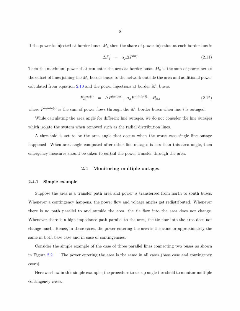
Consider the simple example of the case of three parallel lines connecting two buses as shown

in Figure 2.2. The power entering the area is the same in all cases (base case and contingency

cases).

Here we show in this simple example, the procedure to set up angle threshold to monitor multiple

contingency cases.

9

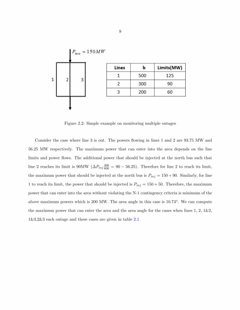
Figure 2.2: Simple example on monitoring multiple outages

Consider the case where line 3 is out. The powers flowing in lines 1 and 2 are 93.75 MW and

56.25 MW respectively. The maximum power that can enter into the area depends on the line

limits and power flows. The additional power that should be injected at the north bus such that

line 2 reaches its limit is 90MW (∆Pinj300800 = 90 − 56.25). Therefore for line 2 to reach its limit,

the maximum power that should be injected at the north bus is Pinj = 150 + 90. Similarly, for line

1 to reach its limit, the power that should be injected is Pinj = 150 + 50. Therefore, the maximum

power that can enter into the area without violating the N-1 contingency criteria is minimum of the

above maximum powers which is 200 MW. The area angle in this case is 10.74o. We can compute

the maximum power that can enter the area and the area angle for the cases when lines 1, 2, 1&2,

1&3,2&3 each outage and these cases are given in table 2.1

10

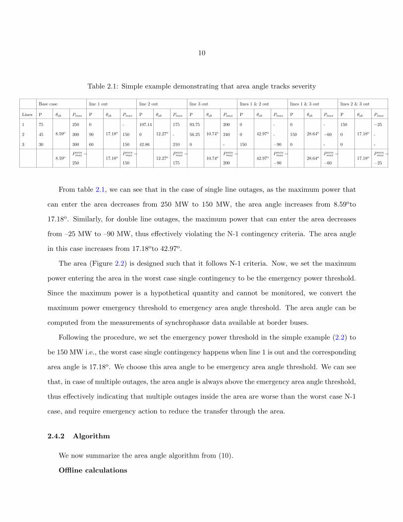
Table 2.1: Simple example demonstrating that area angle tracks severity

Base case line 1 out line 2 out line 3 out lines 1 & 2 out lines 1 & 3 out lines 2 & 3 out

Lines P θab Pmax P θab Pmax P θab Pmax P θab Pmax P θab Pmax P θab Pmax P θab Pmax

1 75

8.59o

250 0

17.18o

- 107.14

12.27o

175 93.75

10.74o

200 0

42.97o

- 0

28.64o

- 150

17.18o

−25

2 45 300 90 150 0 - 56.25 240 0 - 150 −60 0 -

3 30 300 60 150 42.86 210 0 - 150 −90 0 - 0 -

8.59oPminmax =

25017.18o

Pminmax =

15012.27o

Pminmax =

17510.74o

Pminmax =

20042.97o

Pminmax =

−9028.64o

Pminmax =

−6017.18o

Pminmax =

−25

From table 2.1, we can see that in the case of single line outages, as the maximum power that

can enter the area decreases from 250 MW to 150 MW, the area angle increases from 8.59oto

17.18o. Similarly, for double line outages, the maximum power that can enter the area decreases

from –25 MW to –90 MW, thus effectively violating the N-1 contingency criteria. The area angle

in this case increases from 17.18oto 42.97o.

The area (Figure 2.2) is designed such that it follows N-1 criteria. Now, we set the maximum

power entering the area in the worst case single contingency to be the emergency power threshold.

Since the maximum power is a hypothetical quantity and cannot be monitored, we convert the

maximum power emergency threshold to emergency area angle threshold. The area angle can be

computed from the measurements of synchrophasor data available at border buses.

Following the procedure, we set the emergency power threshold in the simple example (2.2) to

be 150 MW i.e., the worst case single contingency happens when line 1 is out and the corresponding

area angle is 17.18o. We choose this area angle to be emergency area angle threshold. We can see

that, in case of multiple outages, the area angle is always above the emergency area angle threshold,

thus effectively indicating that multiple outages inside the area are worse than the worst case N-1

case, and require emergency action to reduce the transfer through the area.

2.4.2 Algorithm

We now summarize the area angle algorithm from (10).

Offline calculations

11

1. Choose the border buses of an area such that the border buses form a cutset (section 2.2).

2. For each single outage inside the area, after the outage, calculate the maximum power that

can enter the area before the first line limit is encountered. The maximum power that can

enter the area for the worst case single outage is the emergency threshold for the maximum

power entering the area. Also define the alarm threshold on the maximum power entering

the area.

3. Set the base case power entering the area to the emergency threshold of the maximum power.

Then for all single outages inside the area, calculate the area angle after the outage.

4. After eliminating the exceptional outages, choose the minimum of all the maximum powers

from step 2 as the emergency power threshold (This is because this is the maximum amount of

power that can enter into the area under worst case single contingency without violating N-1

contingency criteria). The corresponding area angle will be emergency area angle threshold.

Online implementation

1. Continuously observe the system using synchrophasors at the border buses. Get the values

of voltage angles from the synchrophasors in real time.

2. Calculate the area angle using the weights computed offline.

3. If outages which are causing local power redistribution problems have not occurred, then

compare the area angle to its thresholds to take no action or to take proper action with the

appropriate urgency.

4. If the area angle is above the emergency area angle threshold (it implies that the multiple

outages are worse than worst case single line contingency and not following the N-1 criteria),

then take emergency actions to reduce the power in the tie lines of the area.

12

2.5 Exceptional outages

It is not always the case that the area angle is inversely related to the maximum power that

can enter the area. In our experience we encountered some cases in which there are exceptional

outages for which the area angle does not necessarily track the maximum power that can enter into

the area. In (10), Darvishi explained one illustrative example of an exceptional outage where the

area angle increases but the maximum power entering the area remains the same for the simple

network of Figure 2.3. Here we show additional cases by changing the susceptance and line limit

values for the same illustrative example.

The various possibilities of exceptional outages are given in table 2.2. In order to explain

Table 2.2: The possibilities of exceptional outages

Pmaxinto θab

Decreases Constant

Increases Constant

Constant Decreases

Constant Increases

Decreases Decreases

Increases Increases

Constant Constant

all the possibilities of exceptional outages in table 2.2, consider the following network in Figure

2.3. The line limits are chosen such that the network satisfies the N-1 criteria. In this network the

power entering into the area (bus 1) is 100 pu and is always the same in base case and in case of

contingencies. However, the maximum power that can enter into the area changes. The power out

is 80 pu and load is 20 pu in all the cases. By changing the limits and susceptances of the lines

inside the area, we can demonstrate all the possible exceptional cases as shown in table 2.3. The

single line outages which are not following the inverse relation are exceptional outages. This more

general analysis of exceptional outages should be useful in understanding cases in which the area

angle does not work as expected.

13

Figure 2.3: Simple network for illustrating exceptional outages

Table 2.3: Exceptional outages in simple network

Plimit12 b12 Plimit13 b13 Plimit23 b23

line 12 out line 13 outPmaxinto θ13

Pmaxinto θ13 Pmax

into θ13

100 40 100 30 80 20 100 3.3 100 6.5 constant increases

100 50 120 30 80 60 120 3.3 100 3.3 decreases constant

100 50 120 20 80 60 120 5 100 3.3 decreases decreases

100 50 100 20 80 60 100 5 100 3.3 constant decreases

120 50 100 30 100 60 100 3.3 120 3.3 increases constant

120 40 100 30 100 20 100 3.3 120 6.5 increases increases

100 50 100 30 80 60 100 3.3 100 3.3 constant constant

14

CHAPTER 3. DESCRIPTION OF POWER SYSTEM NETWORK MODEL

The data used for modeling and simulation is the North American Western interconnection

(WECC) system. The details and the difference between reduced and detailed model are given in

table 3.1. The network formed is given in Figure 3.1. The top part of the graph corresponds

Table 3.1: Difference between the reduced model and detailed model

Detailed model Reduced model

Number of buses 20194 1553

Number of loads 10951 898

Number of transmission lines 16912 2115

Number of generators 4254 493

Number of two winding transformers 7654 243

Number of three winding transformers 561 0

Number of HVDC lines 3 0

Number of areas 239 64

to those buses which are in Canada followed by those buses which are in Washington, Montana,

Oregon, Idaho, Nevada, Utah, Colorado and the bottom part of graph corresponds to buses which

are in southern California, Arizona. The DC load flow voltage angle is computed for all the buses

in the network and these are shown by the colors in Figure 3.1. It can be seen that angle is higher

at northern buses and tends to reduce as one progresses towards the south, indicating that power

is transferred from northern part of Washington state (where there is generation available) to load

parts such as south western part of California (where there are major load centers) with some power

consumed in between. In this thesis, we explain the area angle concepts on Southern California

region and Southern Idaho region that are essentially load areas, and the BPA area which covers

the states of Washington, Oregon and part of Idaho. The BPA area acts as transmission corridor

transferring power from Canada to California.

15

Figure 3.1: Angles at the buses plotted on WECC. The black color represents a higher value and

blue color represents a lower value

16

CHAPTER 4. AREAS, AREA ANGLES AND THRESHOLDS

We calculated the area angle and set the thresholds on area angles for three different areas. Two

areas in Idaho and in Southern California are load areas. The third area is a transmission corridor

through the states of Washington and Oregon supplying power from Canada down to California.

4.1 Idaho Area Simulation

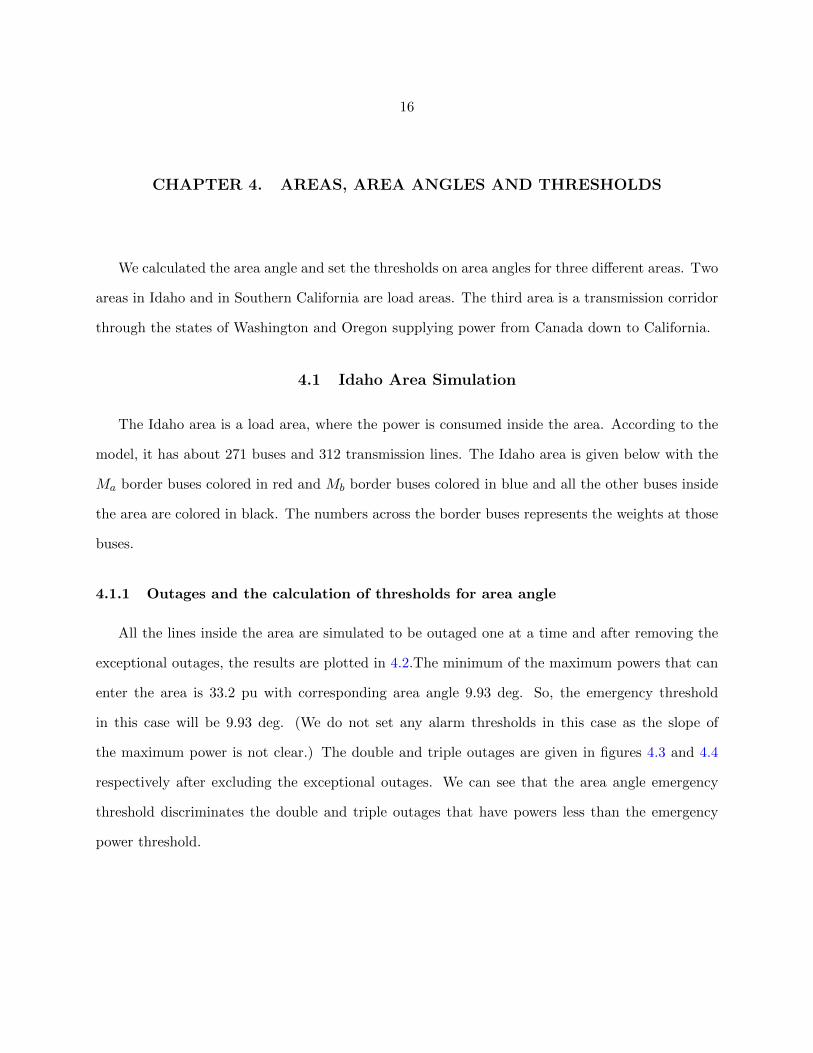
The Idaho area is a load area, where the power is consumed inside the area. According to the

model, it has about 271 buses and 312 transmission lines. The Idaho area is given below with the

Ma border buses colored in red and Mb border buses colored in blue and all the other buses inside

the area are colored in black. The numbers across the border buses represents the weights at those

buses.

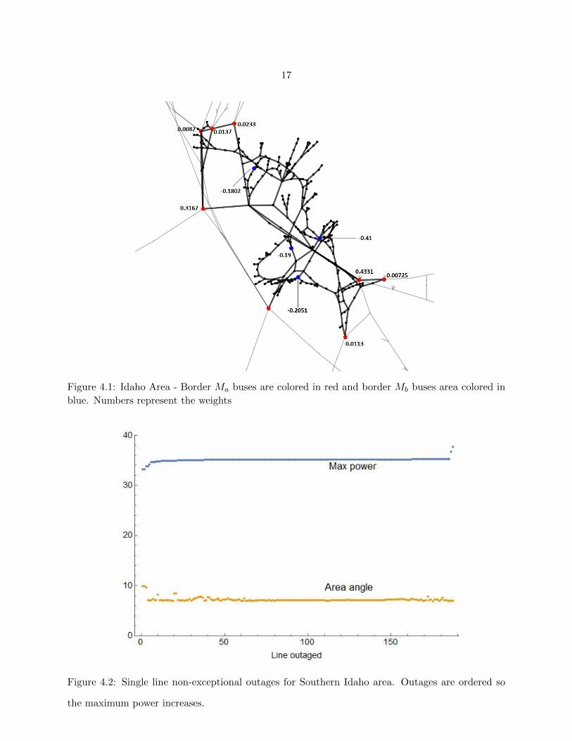
4.1.1 Outages and the calculation of thresholds for area angle

All the lines inside the area are simulated to be outaged one at a time and after removing the

exceptional outages, the results are plotted in 4.2.The minimum of the maximum powers that can

enter the area is 33.2 pu with corresponding area angle 9.93 deg. So, the emergency threshold

in this case will be 9.93 deg. (We do not set any alarm thresholds in this case as the slope of

the maximum power is not clear.) The double and triple outages are given in figures 4.3 and 4.4

respectively after excluding the exceptional outages. We can see that the area angle emergency

threshold discriminates the double and triple outages that have powers less than the emergency

power threshold.

17

Figure 4.1: Idaho Area - Border Ma buses are colored in red and border Mb buses area colored in

blue. Numbers represent the weights

Figure 4.2: Single line non-exceptional outages for Southern Idaho area. Outages are ordered so

the maximum power increases.

18

Figure 4.3: Random sample of 1700 double line non-exceptional outages for Southern Idaho area

Figure 4.4: Random sample of 1396 triple line non-exceptional outages for Southern Idaho area.

19

4.2 Southern California Area

The Southern California is a load area with power transferred through an outer border and

consumed inside the area. The Southern California area network buses and transmission lines are

shown in Figure 4.5.

Figure 4.5: Southern California Area

The Southern California area consists of Los Angeles and regions surrounding Los Angeles and

is shown by the darker buses and lines in Figure 4.5. The Southern California area network has

418 buses and 501 lines. Red buses in Figure 4.5 represent the outer border buses and blue buses

are major loads in Los Angeles. Here we are assuming synchrophasor measurements are available

at the specified buses. As of 2010, synchrophasors were installed or proposed at all the border

buses except for one of the load buses. The trend is for synchrophasor measurements to become

more widespread, particularly as modern relays can include synchrophasor measurements. We note

20

in computing the area angle that border buses with very small weights can be omitted from the

calculation so that synchrophasor measurement at those buses is not required.

4.2.1 Outages and area angle thresholds

The single line outages are given below.

Figure 4.6: Single line non-exceptional outages for Southern California area. Outages are ordered

so that maximum power increases

The power entering the area during the worst case single contingency is approximately 93 pu

and the corresponding area angle is 58 pu (approximately). The double and triple outages are

given below with the emergency thresholds for area angle and max power and it can be seen that

the thresholds clearly detect the double and triple outages which are worse than worst case single

contingency.

21

Figure 4.7: Random sample of 512 double line non-exceptional outages for Southern California

area.

Figure 4.8: Random sample of 2020 triple line non-exceptional outages for Southern California

area.

22

4.3 Robustness to changing stress direction

When determining the area angle thresholds, it is necessary to choose a pattern of stress by

which the power transfer is increased. When a line is out, the participation factors for all the

remaining lines are calculated with respect to power injections at the border buses. The maximum

power that can be injected across the border buses such that line k inside the area reaches its limit

is obtained by dividing the limit of that line by its participation factor according to equation (4) in

(10). Then the amount of power to be injected into the border buses is the minimum of injections

across all the lines. The amount of power to be injected at the border bus such that line k reaches

its maximum power limit depends on the generation shift factor of line k. According to equation

(8) in (10) the generation shift factor for line k with respect to injections at border buses is given

by

ρab(i)k = bk(eTu − eTv )((Bi)−1)(ea − eb)

Here ea and eb are n × 1 vectors (n is the number of buses) with values only at the positions of

border buses and the rest are zero. We choose the values in these column vectors to specify the

pattern of stress. The first method is to choose ea and eb according to the weights at the buses.

The second method chooses ea and eb according to α = Pintoj/Pintom. The pattern of stress is

defined by how the border buses participate in changes in the power transfer.

We compare these two different methods of stressing each area to assess the robustness of the

thresholds when the power stress pattern is changed.

1. The first method increases the power at border bus i proportional to the power injected at

border bus i from outside the area.

2. The second method increases the power at border bus number i proportional to the area angle

weight wi.

23

Figure 4.9: Single line outages for reduced BPA network. Pattern of stress used here is according

to weights at the buses

Here we compare the single line outages of BPA network in a reduced network. Single line

outages for the reduced BPA area from (10) is reproduced here for easy reference in Figure 4.9.

The outages are ordered according to increasing amount of maximum power transfer into the area.

The results in (10) for the north-south transfer of power through the BPA area are obtained with

the second method, so here we give the results for the first method1. The weights at the border

buses used for stressing the system in (10) are

w = {0.23, 0.0057, 0.0078, 0.1, 0.18, 0.017, 0.6,

−0.03,−0.4,−0.38,−0.18,−0.004} (4.1)

The weights at the border buses which are proportional to tie line flows are

α = {0.68, 0.0111, 0.002, 0.056, 0.019, 0.042, 0.18,

−0.002,−0.4,−0.35,−0.23,−0.029} (4.2)

We note the substantial difference in the weights in (4.1) and (4.2).

The single outages of the system stressed according to α are given in Figure 4.10. Comparing

Figure 4.10 with Figure 4.9 we can see that the results are similar and the thresholds do not depend

on the method of stress.1 The first method is described by equation (8) of (10). However the results presented in (10) tacitly use the

second method.

24

Figure 4.10: Single line outages for reduced BPA network. Pattern of stress used here is proportional

to the tie line power flows into the buses.

4.4 Effect of exceptional outages

The formulation of the areas is such that power enters into the area through one set of border

buses and transfers or get consumed at the other set of border buses. The radial lines inside the

area do not participate in the power transfer. The meshed lines in the area can participate in

the power transfer. There is a general tendency for an outage of one the meshed lines to decrease

the maximum power that can be transferred through the area, since the outage tends to transfer

more power to the parallel paths. Moreover, the outage tends to increase the impedance across the

area while the power transfer remains constant. Since the area angle obeys circuit laws, it follows

that the area angle generally increases. Thus there is generally an inverse relationship between

area angle and maximum power transfer that we exploit in the monitoring. However, there are

some exceptional cases in which the area angle does not respond inversely to the maximum power

transfer. These exceptional cases usually correspond to local power redistribution problems as

explained in (10) and further in Chapter 3 of this thesis. Depending on the nature of the lack

of response, some of the lines giving exceptional outages need to be independently monitored to

improve the accuracy of the interpretation of the area angle changes. Fig. 4.11 shows all the single

25

line outages for the Idaho area, including the exceptional outages shown as red dots. Fig. 4.12

shows all the triple line outages for the Idaho area that include at least one exceptional outage.

Figure 4.11: All single line outages for Idaho area with exceptional outages colored in red

Figure 4.12: Random sample of triple line outages for Idaho area with exceptional outages colored

in red

26

CHAPTER 5. CONCLUSION

Our overall philosophy to extract actionable information from synchrophasor data is to restrict

the problem to one pattern of stress for one phenomenon, and suitably combine data from multiple

synchrophasors into a meaningful scalar to be monitored. This restriction of the problem then

allows not only detection of emergency conditions when the scalar exceeds a threshold, but specific

mitigation actions to correct the problem. For example, we use an area angle to monitor a specific

power transfer through a specific area with respect to thermal limits in (10) and monitor with a

scalar index a specific transmission corridor with respect to voltage collapse in (15).

To advance and make workable this philosophy for area angles monitoring thermal limits inside

an area, it is necessary to develop the art of choosing areas and power transfers stressing these

areas, and show that meaningful thresholds can be developed. In this thesis, we extend the area

angle monitoring to a different sort of area in which the power flows from the border of the area

into large loads well inside the area. The emergency thresholds for area angle developed in relation

to the N-1 criterion seem effective in discriminating the triple outages that require no quick action

from those that require quick emergency action to curtail the power transfer. In the case of BPA

area which acts as transfer path area, the initial results suggest that thresholds cannot be set up.

We also briefly assess the performance of the area angle with respect to power stress direc-

tion. We have a choice of stressing the system either according to the weights or according the

proportional tie line power flows. The maximum power that can enter the area remained the same

irrespective of the type of the stress and the emergency thresholds that are setup discriminates the

multiple outages.

The time required to run the offline algorithm of calculating and setting up the thresholds will

be in the magnitude of days if computed by brute force methods. The techniques introduced ()

helped achieve computational efficiency. Even after employing these techniques, the time required

27

for offline algorithm varies from hours to days depending on the size of the area. Online algorithm

calculations are fast since these depend on the voltage angle measurements from the synchrophasors

at the border buses of the area.

This thesis explored setting up thresholds for transfer path areas and load areas. For future

work, this method should be tested on the generation area. In case of load areas, the loads are

assumed to be constant. The effect of dynamic loads on the area angle and thresholds can be

studied. The method is far from perfect in terms of computational time for offline calculations.

more efficient computation can be achieved by utilizing the inbuilt functions of software in which

the algorithms are written.

Our testing of area angle extends the capability to combine synchrophasor measurements into

a scalar index to monitor a specific problem and determine if emergency action needs to be taken

or not. This fast action based on synchrophasor measurements is particularly useful for multiple

contingencies when it is possible that the state estimator may not converge.

I gratefully acknowledge access to the WECC power flow data that enabled this research. The

analysis and conclusions are strictly those of the author and not of PSerc, WECC, DOE, or SCE.

28

REFERENCES

[1] I. Dobson, M. Parashar, A cutset area concept for phasor monitoring, IEEE PES General

Meeting, Minneapolis, MN USA, July 2010.

[2] A. Darvishi, I. Dobson, A. Oi, C. Nakazawa, Area angles monitor area stress by responding to

line outages, North American Power Symposium, Manhattan KS, Sept. 2013.

[3] I. Dobson, Voltages across an area of a network, IEEE Transactions on Power Systems, vol.

27, no. 2, May 2012, pp. 993-1002.

[4] I. Dobson, M. Parashar, C. Carter, Combining phasor measurements to monitor cutset angles,

Forty-third Hawaii International Conference on System Sciences, Kauai, Hawaii, January 2010.

[5] I. Dobson, M. Parashar, A cutset area concept for phasor monitoring, IEEE PES General

Meeting, Minneapolis, MN USA, July 2010.

[6] G.J. Lopez, J.W. Gonzalez, R.A. Leon, H.M. Sanchez, I.A. Isaac, H.A. Cardona, Proposals

based on cutset area and cutset angles and possibilities for PMU deployment, IEEE PES Gen.

Meeting, San Diego CA, July 2012.

[7] I. Dobson, New angles for monitoring areas, IREP Symposium, Bulk Power System Dynamics

and Control - VIII, Buzios, Brazil, Aug. 2010.

[8] A. Darvishi, I. Dobson, Synchrophasor monitoring of single line outages via area angle and

susceptance, North American Power Symposium, Pullman WA USA, September 2014.

[9] 2013 WECC Path Reports, WECC staff, September 2013

29

[10] A. Darvishi, I. Dobson, Threshold-based monitoring of multiple outages with PMU measure-

ments of area angle, IEEE Transactions on Power Systems, vol.31, no.3, May 2016, pp. 2116-

2124.

[11] Mathew P. Oommen, J.L. Kohler, Effect of three winding transformer models on the analysis

and protection of mine power systems. IEEE Transactions on Industry applications, vol. 35,

Issue 3, pp. 670-674.

[12] H. Sehwail, I. Dobson, Locating line outages in a specific area of a power system with syn-

chrophasors, North American Power Symposium (NAPS), Urbana-Champaign IL, Sept. 2012.

[13] H.Sehwail, I.Dobson, Applying synchrophasor computations to a specific area, IEEE Trans.

Power Systems, vol 28, no 3, Aug 2013, pp. 3503-3504.

[14] J.E. Tate, T.J. Overbye, Line outage detection using phasor angle measurements, IEEE Trans.

Power Syst.,vol.23,no.4, Nov.2008, pp.1644-1652.

[15] L. Ramirez, I. Dobson, Monitoring voltage collapse margin with synchrophasors across trans-

mission corridors with multiple lines and multiple contingencies, IEEE Power and Energy

Society General Meeting, Denver CO, July 2015.

30

APPENDIX. SYSTEM MODELLING AND COMPUTATION

As described in the previous chapters, all the simulations are run on a twenty thousand bus

Western Interconnection (WECC) system and all the calculations are done using Mathematica

software. This chapter describes the modeling and steps to improve the computational efficiency.

The data available for simulation is in the PSLF epc format. We have the choice of running DC

load flow either in PSLF or PSSE software and export the necessary details for further calculations

in any format supported by Mathematica. Since we have the framework set up to read PSSE .raw

file format in Mathematica, we exported the .epc file as a .raw file.

A detailed system is always challenging in terms of modeling, computational efficiency, data

analysis etc. Techniques are employed to reduce the computational time and memory required for

computations. In the offline calculations testing area angle and setting thresholds, line outages

have to be simulated. Whenever a line is out, the network topology changes and the susceptance

matrix changes. In the calculation of participation factor, inverse of susceptance matrix is used as

shown in equation 2.8. The network has approximately 20000 buses, so the susceptance of network

is a matrix with 20000 rows and 20000 columns. Inverse calculation of such a matrix involves huge

computational time and memory. We use the matrix inversion lemma to calculate the inverse of

such a huge matrix and this is further explained in section . We achieved better computational

time efficiency by utilizing many of the inbuilt functions in Mathematica. The computational time

and memory required to simulate the area depends on the size of the area.

Branches

The DC power flow is given by the equation

P = Bθ (.1)

31

where Pn×1 is the column vector of power injections at the n buses, θn×1 is a column vector of

voltage angle at the buses, and Bn×n is the admittance matrix where

Bii = −k∑

n=1

bin (.2)

Bik = −bik (.3)

and bik is the susceptance of the line joining bus i and bus k. In the DC load flow, all the branches

are considered lossless. Therefore all the two winding transformers and transmission lines are

represented with series impedance z = r + jx, b = −1x .

Three winding transformers

A three winding transformer modeling is different from a two winding transformer. While

modeling a three winding transformer, we have the choice of a three bus equivalent model or a four

bus equivalent model as shown in Figure .1. In the three bus model, the three winding transformer

is split into two transformers. It does not consider the impedance of primary winding. In the four

bus equivalent, it is split into three two-winding transformers. For the DC load flow calculation,

the primary impedance can be ignored. Therefore, for the DC load flow calculations, the three bus

equivalent is used to model the three winding transformer.

HVDC lines

In the western interconnection, there are three HVDC connections

1. Eastern Alberta Transmission line, which is 485 km long interconnecting Newell HVDC static

inverter plant near Brooks, Alberta with Heathfield static inverter plant near Gibbons, Al-

berta.

2. Pacific DC Intertie, also called Path 65, is 846 miles long interconnecting Celilo converter

station in Oregon to Sylmar converter station north of Los Angeles.

32

Figure .1: Modeling of three winding transformer

3. Intermountain HVDC power line, also called Path 27, is 488 miles long interconnecting Ade-

lanto converter station in Adelanto, California to Intermountain converter station in Delta,

Utah.

In order to model the HVDC lines, we remove power from those buses where HVDC power is

injected and add power to those buses where HVDC power is extracted. In other words, if Pdc is

the amount of power that is transferred through the HVDC line from bus a to bus b, then at bus

a, the injection will be −Pdc and at bus b, the injection will be Pdc.

33

Participation factor calculation

The area angle computation and the setting of area angle threshold helps us discriminate the

double and triple line outages which are comparable to worst case single line outage. The shift

factor of each line inside the area with respect to the border buses of the area is given by equation

(2.8), which is copied here as

ρab(i)k = bk(eTu − eTv )((Bi)−1)(ea − eb) (.4)

Here ea and eb have nonzero entries corresponding to buses Ma and Mb. eu and ev have entry 1 at

the starting bus position and ending bus position of line k respectively.

After choosing a particular area, the values and positions of elements in the column matrices

ea and eb do not change since they are ratios of base power injections at the border buses. The

values of row matrices eTu and eTv do not change but the positions change according to the starting

and ending buses of line k. However, these positions are within range of buses in the area since

the area angle is computed only for the chosen area and all the values at the positions outside the

range of area buses are zero. The structure of the matrices is given below

eTu − eTv = [ 0 0 ··· 0 v1 v2 ··· vk 0 ··· 0 0 ]

((Bi)−1)(ea − eb) =

x1

x2...

xn

(eTu − eTv )((Bi)−1)(ea − eb) = 0 ∗ x1 + 0 ∗ x2 + · · ·+ v1 ∗ xb1 + v2 ∗ xb2 + · · ·+ vk ∗ xbk + · · ·+ 0 ∗ xn

From the above equations, we can see that in the participation factor calculation, only the elements

of the Binverse matrix whose positions are within the range of area buses are required. Hence we

can form a sparse Binverse matrix which has elements only in the range of buses of the chosen area

34

and all other elements allowed to be zero. This not only reduces the memory to store the Binverse

matrix but also increases efficiency in calculation of participation factor.

B inverse matrix calculation

To calculate the participation factor during single, double, and triple outages, it is necessary

to calculate B−1out matrix for each outage i. We calculate the B−1

out matrix from the matrix inverse

lemma.

eij =

0

...

1

...

−1

...

0

Bout = B + bijeijeTij (.5)

Here Bout is the B matrix after line k is out. eij has 1 at the starting bus position of line k and

−1 at the ending bus position. bij is the susceptance of the line k with starting and ending bus

positions at i and j respectively.

From the matrix inversion lemma

(B + cdT )−1 = B−1 −B−1c(IM + dTB−1c)−1dTB−1 (.6)

where B is an n× n matrix, c and d are n×m matrices and I is an m×m Identity matrix.

Applying the Matrix inversion lemma to our problem results in the calculation of B−1out from base

case B−1 matrix:

B−1out = B−1 −

B−1bijeijeTijB

−1

1 + bijeTijB−1eij

(.7)

35

Here B−1 is the base case pseudoinverse of the B matrix with elements only in the positions which

are in the range of area buses.