Three Lectures on: Control of Coupled Fast and Slow Dynamics · Three Lectures on: Control of...

1

Three Lectures on:

Control of Coupled Fast and Slow Dynamics

Zvi Artstein

Ravello, September 2012

2

Control of Coupled Fast and Slow Dynamics

Zvi Artstein

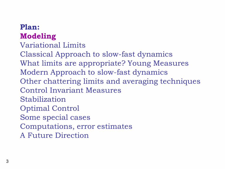
Plan:

Modeling

Variational Limits

Classical Approach to slow-fast dynamics

What limits are appropriate? Young Measures

Modern Approach to slow-fast dynamics

Other chattering limits and averaging techniques

Control Invariant Measures

Stabilization

Optimal Control

Some special cases

Computations, error estimates

A Future Direction

3

Plan:

Modeling

Variational Limits






Stabilization

Optimal Control

Some special cases


A Future Direction

Example from real life: Airplane

4

Example from real life: Helicopter

5

Example from real life: The hummingbird

6

7

The framework ODE:

An ordinary differential equation

8

The framework CONTROL:

A control equation

Possible goals:

Bolza Problem

Mayer Problem

9

A reduction of Bolza to Mayer:

The goal

by adding a coordinate and an equation

and seeking minimizing the additional coordinate

can be reduced to

Adolf Mayer

1839 - 1907

Oskar Bolza

1857 - 1942

10

The equivalent differential inclusion:

A control equation

can be written as:

11

How to model coupled slow and fast motions?

12

Tikhonov’s Singular Perturbations model

of coupled slow and fast motions

The perturbed system:

Where: in the slow and in the fast, variables

We are interested in the limit behavior of the

system as

The fast part can be written as:

13

A mathematical example capturing reality:

An elastic structure in a rapidly flowing nearly invicid

fluid (with Marshall Slemrod)

http://www.math.wisc.edu/~apache/gallery/foto/slemrod.jpg

14

To make the long story short:

Based on a model of Iwan/Belvins and Dowel/Ilgamov,

the limit (after normalization) equations:

van der Pol oscillatora generator of a With

15

An example – Relaxation oscillation

16

Singularly perturbed optimal control systems:


Of interest: The behavior of the system as

17

Applications

A variety of natural phenomena and engineering design.

The latter include: Regulation, LQ-Systems, Feedback Design, Stabilization, Robustness, Stochastics, Filters, Optimal Control, Hydropower Production, Nuclear Reactions, Aircraft Design, Flight Control, and many more !

The classical approach to handle the applications is the model-reduction - after Levinson-Tikhonov in the differential equations trait and after Kokotovic in the control Setting

18

Other coupled slow and fast dynamics

19

Plan:

Modeling

Variational Limits






Stabilization

Optimal Control

Some special cases


A Future Direction

20

The definition of a variational limit:

Given a system (an equation or a control

equation) with a parameter that tends to a limit.

A variational limit is a system whose solutions

capture the limit behavior of the solutions of the

parameterized system, as the parameter tends to

its limit,

Capture = limit of the trajectories, limit of the

optimal controls, limit of the values

21

Plan:

Modeling

Variational Limits






Stabilization

Optimal Control

Some special cases


A Future Direction

22

The classical Tikhonov order reduction approach

Write the perturbed system as:

The limit behavior as is captured by the system:

23

Norman Levinson Andrei Nikolayevich Tikhonov

1906 -1993 1912 - 1975

24

The geometry of the solution:

25

An example – Relaxation oscillation

26

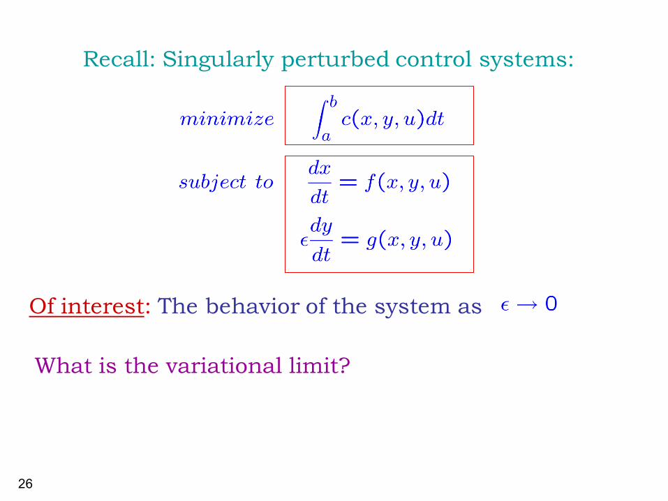
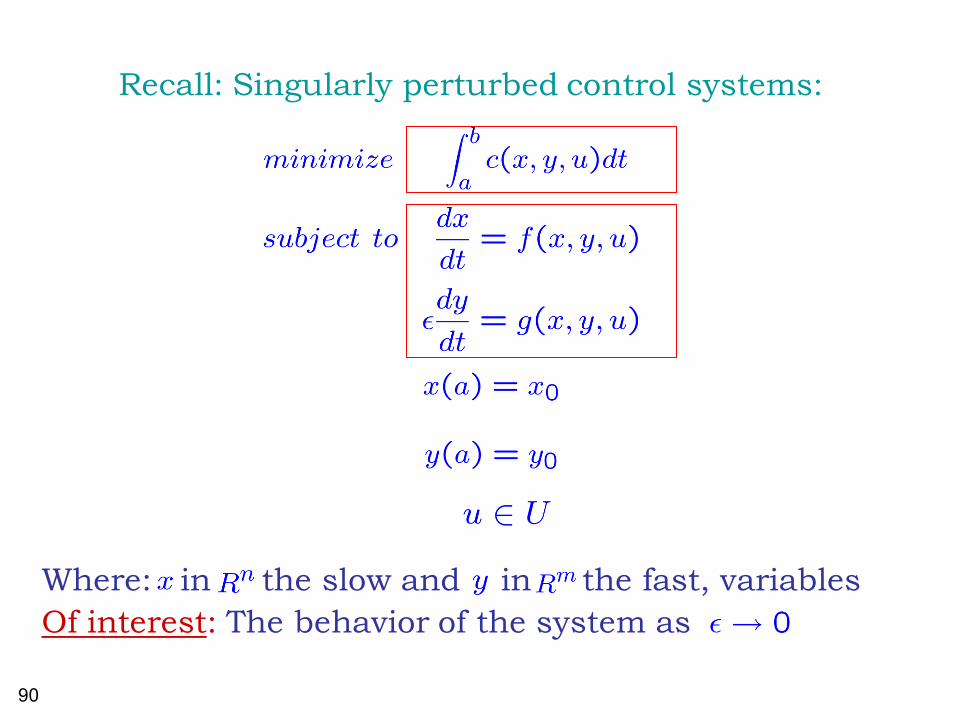
Recall: Singularly perturbed control systems:


What is the variational limit?

27

The limit of:

is

28

Petar Kokotovic

29

The geometry of the solution:

30

BUT

31

The general situation:

There is no reason why the optimal fast solution will converge and not, say, oscillate!

32

This was pointed out in the mid 1980’s, independently,

By

Assen Dontchev and Valadimir Veliov

And by

Vladimir Gaitsgory

33

A mathematical illustration:

Non-stationary relaxation oscillation

34

Recall: A mathematical example capturing reality:

An elastic structure in a rapidly flowing nearly

invicid fluid

35

Numerical results:

The slow dynamics The fast dynamics

Computations by:

Zvi Artstein Jasmine Linshiz Edriss Titi:

Also in Nature: The hummingbird

36

37

An illustration of a control problem:

The questions: when should the switch be made?

How should this be carried out when the speed is

very fast?

38

An example – after V. Veliov 1996

Applying an order reduction (i.e. plugging )

yields zero value. Clearly one can do better!

39

No equilibrium in the limit:

40

The limit solution:

The limit strategy as can be expressed as a bang-bang feedback resulting in:

Limit trajectories The bang-bang feedback

41

Plan:

Modeling

Variational Limits






Stabilization

Optimal Control

Some special cases


A Future Direction

42

Strong limit on a space of functions:

Recall the strong limit in, say L2 :

The strong limit may not work for the variational limit of singular perturbations – recall the examples.

43

Weak limit on a space of functions:

The L2 weak-limit:

The sequence converges weakly to if

The weak limit may not work for the variational limit of singular perturbations – recall the examples.

44

On a space of parameters:

Consider an ordinary differential equation with

parameters

Strong convergence of the parameters implies continuous dependence of solution but is not compact

Weak convergence of the parameters is compact but does not imply continuous dependence

45

Observation:

Continuous dependence and compactness are

opposing properties !

Can we construct a convergence that will have both

properties: continuous dependence of solution and

compactness ?

To the rescue

46

47

Laurence Chisholm Young

July 14, 1905 - December 24, 2000

Cambridge, England, Madison WI, USA

The price:

The limit function will be out of the original space

48

It is called: A Young measure

49

An implicit Definition of a Young Measure:

Let be a sequence of parameter functions

(say bounded from an interval to .

There exist a subsequence (say the sequence

itself) and a family of probability measures

on parameterized by such that for every

right hand side

converges weakly to

50

Proof

Based on (simple) functional analysis arguments

(incorporating weak* convergence and Alaoglu

compactness Theorem).

51

A consequence:

Solutions of the ordinary differential equation with

parameters

converge to solution of the ordinary differential

equation with the Young measure

52

A constructive Definition of a Young Measure:

Let be a metric space

Denote by the family of probability

measures on

Let be another metric space endowed with a

measure (say Lebesgue measure on an interval)

Definition: A mapping from to is a

Young Measure

53

A Pictorial Definition:

54

The structure of the space :

The elements: -additive set-functions from the

Borel subsets onto the unit interval.

Convergence of if

For every continuous and bounded.

Prohorov metric between measures

and is the smallest such that for every Borel set

55

Consequences concerning :

If is complete and separable so is

If is compact so is

56

The structure of Young measures :

Consequences: If is complete and separable so

is the space of Young measures

If is compact so is the space of Young measures

Can be viewed as a “probability” measure on

57

A major property of Young measures:

An ordinary function can be viewed as a Dirac-

valued Young measure.

58

The nature of the convergence

59

For instance:

The sequence

converges to a Young measure with a constant

value, namely the measure on given by

60

Functions are dense in the space of Young Measures !

When the underlying space is without atoms then

any Young measure can be approximated by a function

61

When the limit is a function:

The space of Young Measures completes the space of

functions. What convergence does it reflect if the limit

Young measure happens to be a function?

The limit is then strong ( , , but not )

62

Key properties:

Existence of the limit

Keeping information about the location of the values

Possibility to approximate by an ordinary function

63

Recall the case of a space of parameters:


parameters

Strong convergence implies continuous dependence of solution but is not compact

Weak convergence is compact but does not imply continuous dependence

What happens if converges to a Young

measure?

64

Definition:

Likewise, for an ordinary differential equation

we mean

If and is a probability

measure then

65

Main application:


parameters

Then the solutions of the odes with parameters converge to the solution of the ode with the Young measure

Thus, the convergence to the Young measure is both compact and implies continuous dependence

And converges to a Young measure

66

The key tool:

Consider the right hand side of the ordinary

differential equation with parameters

Then converges weakly to

and converges to a Young measure

67

Plan:

Modeling

Variational Limits






Stabilization

Optimal Control

Some special cases


Future Directions

68

Applications to Control and the

Calculus of Variations

69

An application (after L.C. Young):

70

A problem without a solution:

71

Approximate solutions:

72

Better approximations:

No ordinary limit which is useful !

73

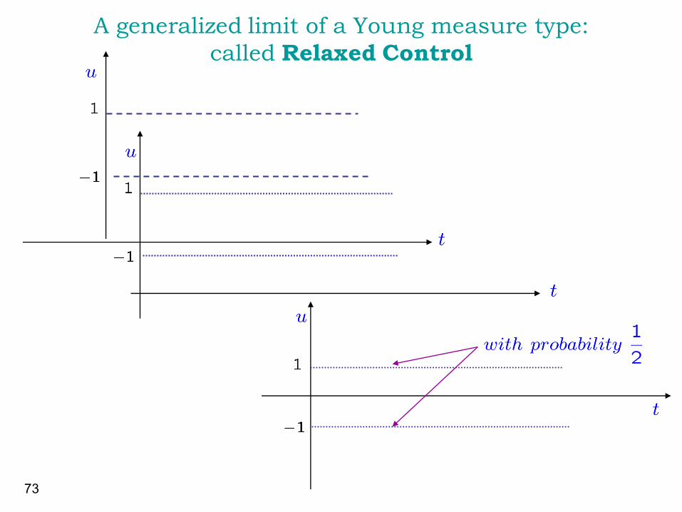
A generalized limit of a Young measure type:

called Relaxed Control

The effect of Relaxed Control:

Convexification of the vector field

Is there a control that makes a solution?

Yes, the control that averages +1 and -1.

74

75

Jack Warga

1922 - 2011

76

A prior appearance in the calculus of variations:

The general problem:

The particular problem without a solution:

77

Generalized curves in the calculus of variations:

For the problem:

A generalized curve is a pair:

satisfying:

The goal:

78

Recall the illustration of a control problem:

The questions: when should the switch be made?

How should this be carried out when the speed is

very fast?

79

In the limit: A distribution arises

80

The limit solution:

The limit strategy as can be expressed as a bang-bang feedback resulting in:

Limit measure The bang-bang feedback

81

Recall: A mathematical example capturing reality:

An elastic structure in a rapidly flowing nearly

invicid fluid

82

Numerical results:

The slow dynamics The fast dynamics

83

Recall: Singular perturbations as a model

of coupled slow and fast motions:

The perturbed system:

We are interested in the limit behavior of the

system as

Equivalently:

84

The classical Tikhonov approach

Write the perturbed system as:

The limit behavior as is captured by the system:

This type of variational limit does not capture the

general situation

85

A program to exploit Young Measures this started by

Zvi Artstein and Alexander Vigodner, 1996.

86


The solution oscillates. The limit (as ) may be described as a Young measure

87


The Young measure is defined on the x-space with values being probability measures on the y-space

88

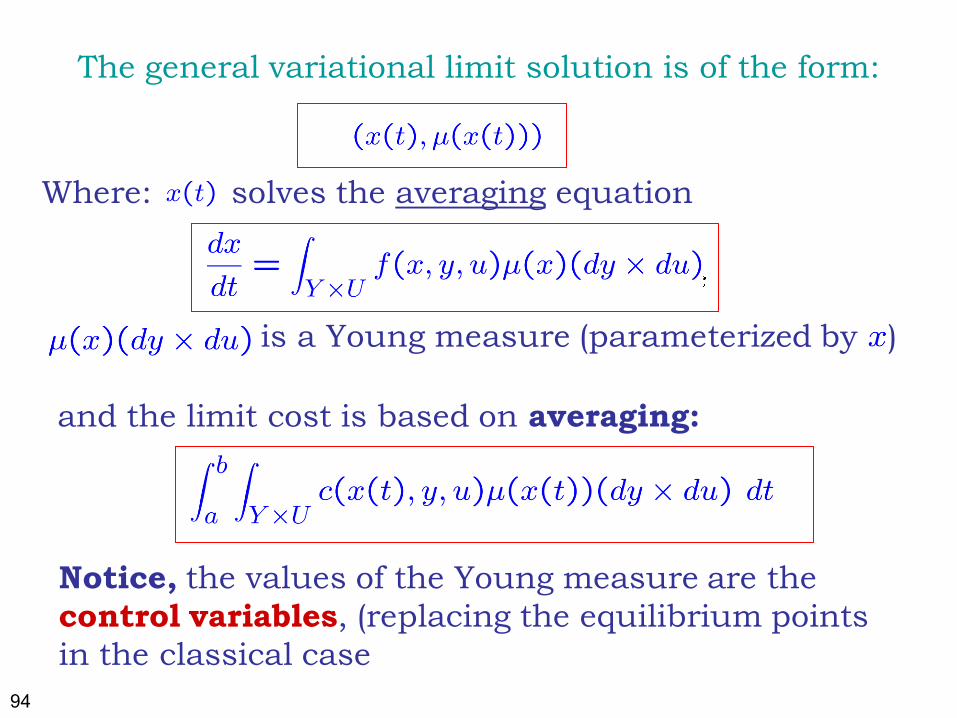
The variational limit solution in the new formulation :

and solves the averaging equation

where is a Young measure

Now to control systems

89

90

Recall: Singularly perturbed control systems:



91

The order reduction method (Petar Kokotovic et al.)

The limit as is depicted by namely, by:

92


There is no reason why the optimal fast solution will converge and not, say, oscillate!

93


The values of the Young measure are:

measures of the (fast state, control) dynamics !

94

The general variational limit solution is of the form:

Where: solves the averaging equation

is a Young measure (parameterized by )

Notice, the values of the Young measure are the

control variables, (replacing the equilibrium points

in the classical case

and the limit cost is based on averaging:

95

The “equivalent” differential inclusion:

solves the differential inclusion

is a Young measure (parameterized by )

Notice, the values of the Young measure are the

control variables, here they determine the velocity

of the slow variable

where

96

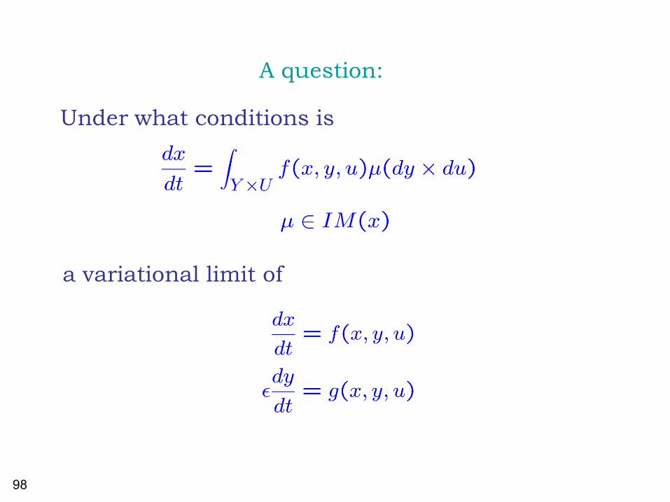
A question:

Could any probability measure be a value for the

Young Measure of the variational limit?

If not, how can the possible values be classified

and identified?

A promise:

We shall soon give a characterization of the

probability measures that may appear as values

in the variational limit.

We denote this family by

97

Recall: A variational limit

What do we want from a variational limit?

1. Convergence of the values

2. Convergence of trajectories

3. Convergence of optimal controls

and

4. Possibility to construct near optimal solution

for the perturbed system given an optimal

solution to the variational limit.

98

A question:

Under what conditions is

a variational limit of

Uniform boundedness and controllability of

solutions of

99

A Theorem:

The conditions are:

The set-valued map

Regularity (modest) of and

is Lipschitz

100

The Lipschitz condition cannot be dropped:

Example (Olivier Alvarez, Martino Bardi):

is a polar coordinate

101

An issue:

How to relate trajectories (say optimal solutions)

of the limit problem to the perturbed problem?

The answer:

If is designed such that

approximates the limit Young Measure (in

the space of Young Measures), the outcome of the

perturbed equation will be a good approximation

of the limit (hence of the optimal solution to the

perturbed equation. Under the conditions of the

theorem his can be done !

102

The End

of lecure 1

Thanks for the attention

See you tomorrow

Three Lectures on: Control of Coupled Fast and Slow Dynamics · Three Lectures on: Control of...

Documents

Transcript of Three Lectures on: Control of Coupled Fast and Slow Dynamics · Three Lectures on: Control of...