
Three Essays on Aligning Supply Chain Strategies with the ...
137
Three Essays on Aligning Supply Chain Strategies with the Business Environment Inauguraldissertation zur Erlangung des akademischen Grades eines Doktors der Wirtschaftswissenschaften der Universität Mannheim vorgelegt von Christian Joachim Freiherr von Falkenhausen Mannheim
Transcript of Three Essays on Aligning Supply Chain Strategies with the ...

Three Essays on
Aligning Supply Chain Strategies
with the Business Environment
Inauguraldissertation
zur Erlangung des akademischen Grades
eines Doktors der Wirtschaftswissenschaften
der Universität Mannheim
vorgelegt von
Christian Joachim
Freiherr von Falkenhausen
Mannheim

ii
Dekan: Prof. Dr. Dieter Truxius
Referent: Prof. Dr. Moritz Fleischmann
Korreferent: Prof. Dr. Christoph Bode
Tag der mündlichen Prüfung: 15. Dezember 2017

iii
Acknowledgements
Moritz Fleischmann, the supervisor of this thesis, and I engaged in our first conversation at the
end of one of his lectures. Since I had arrived late and fallen asleep subsequently, he proposed
that next time I would stay awake and arrive on time. I took his advice to heart, eventually
enrolled in most of his courses, and ultimately discovered a passion for operations management
that led me to take up my doctoral studies at his chair.
During this time, having Moritz as my supervisor was invaluable. His composed and well-
thought-throughout manner provided not only a pleasant working environment, but also much-
needed reassurance when I was unsure how to proceed with my studies. To this day, I am
impressed by how quickly and thoroughly he comprehends the work I present to him and by
the clear-cut guidance he gives concerning matters that require improvement. Most importantly
to me though, over the past three years, I could always rely on Moritz’ backing regarding issues
that extended beyond the immediate needs of our research. Be it visiting a conference, joining
a doctoral course at a different university, or aligning our projects with the timeline we had set
when I joined the chair – knowing that I could confide in my supervisor to have these issues in
mind provided a trustful and motivating basis for the pursuit of this thesis.
I also greatly appreciate the support I have received from Christoph Bode. Christoph has
taught me the basics of empirical research, ranging from the need for theorizing, “setting the
hook”, to practical topics such as the dos and don’ts of writing an empirical research article.
Further, he contributed greatly to my first research project. Christoph was not only a valuable
source of reference regarding methodological questions, he also provided key ideas with
regards to the structure of the article. Having a knowledgeable contact like Christoph only a
knock-on-the-door away was extraordinary – I am truly grateful for his tremendous help.
Moreover, I would like to thank Christian Eich and Thomas Furtwängler for being my
supervisors at BASF. Christian enabled me to set the foundation of my research. He facilitated
access to data and ensured I participate in ongoing initiatives connected to my research.
Thomas, who was my supervisor for the past two years, has played a major role in embedding
my research into the supply chain governance of BASF. Working together with him was
extremely rewarding, as it allowed me to experience first-hand how the approaches developed
in this thesis can contribute to making a difference a practice.

iv
In addition to the aforementioned contributors, there are many colleagues that have made
the past three years exceptional. I will miss the workplace banter and the distractions from day-
to-day work that I have enjoyed with my fellow doctoral students and the strategy development
team at BASF. A special mention goes to Michael Westerburg, who not only excelled at
providing such distractions, but also at giving valuable feedback that helped to improve this
manuscript.
Finally, and most importantly, I am greatly indebted to my family, my girlfriend and my
friends for their continuous encouragement and undoubting support over the past years.
Knowing that I could count on their backing has kept me on track and, hence, rendered the
completion of this undertaking possible. I dedicate this thesis to them.
v
Abstract
Aligning the competitive priorities of supply chains with the requirements of the business
environment is critical for competing successfully in the marketplace. Nonetheless, many
companies fail to develop supply chain strategies that provide a good “fit” to the characteristics
of their business. The goal of the thesis at hand is therefore to provide insights for three steps
that are key for attaining alignment: (1) capturing requirements of the business environment,
(2) subdividing products and customers to obtain segments with distinct supply chain design
requirements and (3) developing aligned supply chains strategies for each segment. The first
study investigates which variables companies should analyse to capture the requirements their
business. Specifically, it tests the effects hypothesized to be underlying the five most frequently
cited contingency variables in the literature on supply chain strategy. The results indicate that
demand variability and the customer lead time requirements are important for setting
competitive priorities because they influence whether companies require market mediation
capabilities to fulfil demand as requested by customers. Volume, variety and lifecycle duration
are less important for this purpose, but may instead be used for analysing the causes of variable
demand. The second study investigates how companies can subdivide a heterogeneous set of
products or customers into groups (“segments”) that require distinct supply chain strategies.
The study uses clustering and classification to form segments quantitatively and compares the
results to segments that were formed based on managers’ tacit knowledge. The findings indicate
that managers may choose segments that do not reflect the needs of their business environment,
consequently pursuing supply chain strategies that adversely affect financial performance.
Clustering and classification help managers detect such segment-environment mismatches and
thus serve as valuable tools for challenging managers’ judgment. Lastly, to facilitate the
derivation of aligned supply chain strategies, the third study investigates in which business
environments companies should prioritize responsiveness, i.e., the ability to fulfil orders within
a time frame that is acceptable to the customer. As the extant literature provides inconsistent
recommendations in this regard, the study analyses both the benefits and the costs of shorter
lead times. The results suggest that responsiveness can increase financial performance in two
distinct ways: either by matching supply and demand or by decreasing supply chain related
costs depending on the characteristics of the products that are being sold.

vi
Contents
Acknowledgements .................................................................................................................. iii
Abstract ..................................................................................................................................... v
List of Figures .......................................................................................................................... ix
List of Tables ............................................................................................................................. x
Chapter 1 Introduction ......................................................................................................... 1
Motivation ...................................................................................................................... 1
Research questions ......................................................................................................... 3
2.1 Research Question 1: Capturing requirements of the business environment........ 4
2.2 Research Question 2: Data-driven supply chain segmentation ............................. 5
2.3 Research Question 3: Performance outcomes of responsiveness ......................... 7
Empirical basis ............................................................................................................... 7
3.1 Data requirements ................................................................................................. 7
3.2 Case company ....................................................................................................... 8
3.3 Data characteristics ............................................................................................... 9
Chapter 2 Contingency variables for developing supply chain strategies:
An analysis of the DWV3 framework ............................................................. 13
Motivation .................................................................................................................... 14
Categorizing contingency variables ............................................................................. 15
2.1 Challenges in the operating environment............................................................ 16
2.2 Value of market mediation .................................................................................. 20
Focus of this study: DWV3 variables ........................................................................... 21
Hypothesis development .............................................................................................. 22
4.1 Conceptual framework ........................................................................................ 22
4.2 Hypothesis ........................................................................................................... 23
Dataset .......................................................................................................................... 25
5.1 Data collection and sampling .............................................................................. 25
5.2 Dependent and independent variables................................................................. 26
5.3 Control variables ................................................................................................. 28
Methodology................................................................................................................. 28
Results .......................................................................................................................... 31
7.1 Endogeneity ........................................................................................................ 31
7.2 Hypothesis testing ............................................................................................... 32
7.3 Direct and indirect effects on reliability ............................................................. 33
Discussion..................................................................................................................... 36
8.1 Demand variability and customer lead time requirements.................................. 36
8.2 Demand volume and product lifecycle duration ................................................. 36
vii
8.3 Product variety .................................................................................................... 37
Conclusion .................................................................................................................... 37
9.1 Implications ......................................................................................................... 37
9.2 Limitations and future research........................................................................... 39
Chapter 3 Supply chain segmentation: A data-driven approach ................................... 41
Motivation .................................................................................................................... 42
Related literature .......................................................................................................... 43
2.1 Qualitative approaches ........................................................................................ 43
2.2 Quantitative approach ......................................................................................... 45
2.3 Clustering ............................................................................................................ 45
2.4 Classification ....................................................................................................... 47
Case company ............................................................................................................... 48
3.1 Company profile ................................................................................................. 48
3.2 Qualitative segments ........................................................................................... 49
Clustering ..................................................................................................................... 50
4.1 Dataset ................................................................................................................. 50
4.2 Segmentation criteria .......................................................................................... 50
4.3 Clustering procedure ........................................................................................... 53
4.4 Assessing cluster solutions ................................................................................. 53
Comparing quantitative and qualitative segments ........................................................ 58
5.1 Mismatch-performance link ................................................................................ 58
5.2 Dataset and variables .......................................................................................... 59
5.3 Endogeneity ........................................................................................................ 60
5.4 Results ................................................................................................................. 61
Classification ................................................................................................................ 62
Discussion and conclusion ........................................................................................... 64
7.1 Implications ......................................................................................................... 64
7.2 Limitations and future research........................................................................... 65
Appendix A ......................................................................................................................... 66
Appendix B .......................................................................................................................... 68
Chapter 4 Performance outcomes of responsiveness:
When should supply chains be fast? ................................................................ 73
Introduction .................................................................................................................. 74
Conceptual model ......................................................................................................... 75
2.1 The responsiveness-performance link ................................................................. 75
2.2 Responsiveness and the market mediation function ........................................... 78
2.3 Responsiveness and the physical function .......................................................... 82
Dataset .......................................................................................................................... 84
3.1 Data collection and sampling .............................................................................. 84
viii
3.2 Dependent and independent variables................................................................. 86
3.3 Control variables ................................................................................................. 87
Methodology................................................................................................................. 88
4.1 Analysis at Level 2 .............................................................................................. 88
4.2 Analysis at Level 1 .............................................................................................. 92
Results .......................................................................................................................... 93
5.1 Responsiveness and the market mediation function ........................................... 96
5.2 Responsiveness and the physical function .......................................................... 98
Discussion and implications ....................................................................................... 102
Limitations and future research directions ................................................................. 107
Chapter 5 Summary, limitations and outlook ................................................................ 109
Summary of the research questions ............................................................................ 109
1.1 Research Question 1: Capturing requirements of the business environment.... 109
1.2 Research Question 2: Data-driven supply chain segmentation ......................... 111
1.3 Research Question 3: Performance outcomes of responsiveness ..................... 113
Limitations .................................................................................................................. 114
Outlook ....................................................................................................................... 115
References ............................................................................................................................. 119
Curriculum Vitae ................................................................................................................. 127
ix
List of Figures
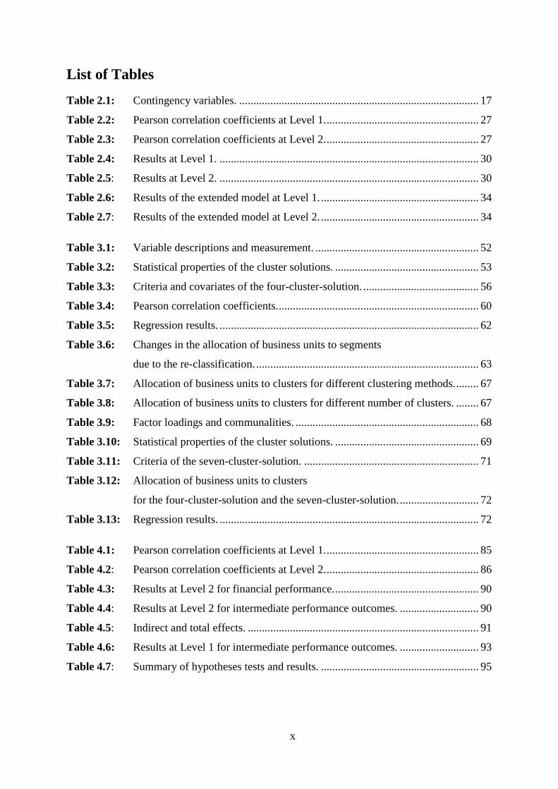
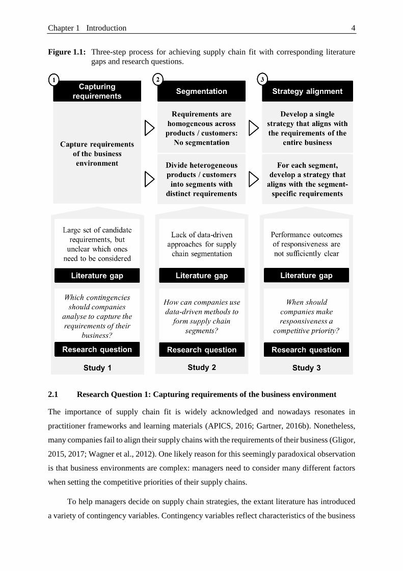
Figure 1.1: Three-step process for achieving supply chain fit. ............................................. 4
Figure 1.2: Data characteristics ............................................................................................. 9
Figure 1.3: Multilevel data structure. .................................................................................. 10
Figure 2.1: Conceptual framework. .................................................................................... 23
Figure 2.2: Multilevel data structure. .................................................................................. 26
Figure 2.3: Extended conceptual framework. ..................................................................... 33
Figure 3.1: Scatter plots of the two-cluster-solution. .......................................................... 54
Figure 3.2: Scatter plots of the three-cluster-solution. ........................................................ 55
Figure 3.3: Scatter plots of the four-cluster-solution. ......................................................... 55
Figure 3.4: Effect of mismatches on financial performance. .............................................. 59
Figure 3.5: Scatter plots of the five-cluster-solution. .......................................................... 69
Figure 3.6: Scatter plots of the seven-cluster-solution. ....................................................... 70
Figure 4.1: Conceptual framework. .................................................................................... 78
Figure 4.2: Moderating effect of demand variability
on the relationship between responsiveness and reliability. ............................. 80
Figure 4.3: Moderating effect of customer lead time requirements
on the relationship between responsiveness and reliability. ............................. 81
Figure 4.4: Multilevel data structure. .................................................................................. 85
Figure 4.5: Moderating effects of challenges in the operating environment
on the relationship between responsiveness and reliability. ............................. 97
Figure 4.6: Moderating effect of contribution margins
on the relationship between reliability and financial performance. .................. 98
Figure 4.7: Moderating effect of customer lead time requirements
on the relationship between responsiveness and inventory at Level 2. ............ 99
Figure 4.8: Moderating effect of challenges in the operating environment
on the relationship between responsiveness and both cost types at Level 1. . 101
Figure 4.9: Scatter plot of contribution margins
and challenges in the operating environment. ................................................ 104
Figure 4.10: Extended and modified version of Fisher's framework. ................................. 104
x
List of Tables
Table 2.1: Contingency variables. ..................................................................................... 17
Table 2.2: Pearson correlation coefficients at Level 1. ...................................................... 27
Table 2.3: Pearson correlation coefficients at Level 2. ...................................................... 27
Table 2.4: Results at Level 1. ............................................................................................ 30
Table 2.5: Results at Level 2. ............................................................................................ 30
Table 2.6: Results of the extended model at Level 1. ........................................................ 34
Table 2.7: Results of the extended model at Level 2. ........................................................ 34
Table 3.1: Variable descriptions and measurement. .......................................................... 52
Table 3.2: Statistical properties of the cluster solutions. ................................................... 53
Table 3.3: Criteria and covariates of the four-cluster-solution. ......................................... 56
Table 3.4: Pearson correlation coefficients. ....................................................................... 60
Table 3.5: Regression results. ............................................................................................ 62
Table 3.6: Changes in the allocation of business units to segments
due to the re-classification. ............................................................................... 63
Table 3.7: Allocation of business units to clusters for different clustering methods. ........ 67
Table 3.8: Allocation of business units to clusters for different number of clusters. ........ 67
Table 3.9: Factor loadings and communalities. ................................................................. 68
Table 3.10: Statistical properties of the cluster solutions. ................................................... 69
Table 3.11: Criteria of the seven-cluster-solution. .............................................................. 71
Table 3.12: Allocation of business units to clusters
for the four-cluster-solution and the seven-cluster-solution. ............................ 72
Table 3.13: Regression results. ............................................................................................ 72
Table 4.1: Pearson correlation coefficients at Level 1. ...................................................... 85
Table 4.2: Pearson correlation coefficients at Level 2. ...................................................... 86
Table 4.3: Results at Level 2 for financial performance. ................................................... 90
Table 4.4: Results at Level 2 for intermediate performance outcomes. ............................ 90
Table 4.5: Indirect and total effects. .................................................................................. 91
Table 4.6: Results at Level 1 for intermediate performance outcomes. ............................ 93
Table 4.7: Summary of hypotheses tests and results. ........................................................ 95
Chapter 1 Introduction 1
Chapter 1 Introduction
Motivation
Contingency theory states that in order to maximize performance, companies need to align the
structures of their organization with the context they operate in (Donaldson, 2001; van de Ven
et al., 2013). The strategic management literature refers to the alignment between strategy and
environment as “fit” (Venkatraman, 1989). The need to achieve “fit” between strategy and
context is also widely recognized in the supply chain community (Sousa and Voss, 2008).
Following the seminal article by Fisher (1997), a thrust of studies has highlighted the adverse
effects of failing to align supply chain strategies with the requirements of the business
environment (Childerhouse et al., 2002; Christopher et al., 2009; Lee, 2002; Qi et al., 2009;
Randall and Ulrich, 2001). There are indeed many real-word examples where misalignment has
eroded companies’ market positions.
Consider, for instance, the well-known case of Gap Inc. and Inditex S.A. Both companies
operate in the fashion industry, i.e., a business environment where demand is hard to forecast
because consumer preferences change quickly (Christopher et al., 2004). Despite operating in
the same industry, the two companies pursue radically different supply chain strategies. Gap,
on the one hand, orders products up to one year in advance (CNN, 2016). Inditex, on the other
hand, pursues a strategy that emphasizes short lead times. At Zara, Inditex’ most prominent
fashion brand, the time between the design of a new product and its arrival in stores can be as
short as 15 days (Ferdows et al., 2004).
Since Inditex achieves these short lead times by relying on local production, frequent
replenishments at stores, and the use of fast transportation modes, it incurs comparably high
production and transportation costs (Chopra and Sodhi, 2014). Nonetheless, pursuing short lead
times pays off for Inditex. Short lead times are important in the fashion industry, since they
allow companies to operate with lower inventories and generate additional revenues by offering
the latest trends (The Economist, 2015). Because Inditex’ supply chain strategy therefore
closely matches the requirements of its business environment, the company has continuously
gained market share over the past years (Reuters, 2017a). On the contrary, Gap has lost market
share and struggles to be profitable (Forbes, 2015). Recently, the company has launched an
initiative to reduce cycle times with the goal of reacting to changes in customer preferences
more quickly (CNN, 2016).
Chapter 1 Introduction 2
Yet while a supply chain strategy that emphasizes flexibility and short lead times may be
successful in the fashion industry, it does not guarantee success in other business environments
as well. Consider, for instance, two of the largest bankruptcies in Germany that took place in
the past decade: the semiconductors manufacturer Qimonda AG and the photovoltaics
manufacturer Solarworld Industries AG (Amtsgericht Bonn, 2017; Amtsgericht München,
2009). Both companies had opened production facilities close to their customers in high-cost
countries during a period of high market growth (Infineon Technologies AG, 2006; Solarworld
Industries AG, 2009). However, for these companies, the benefits of local production did not
outweigh the associated costs. When their respective markets saturated and the margins for their
products dropped, Qimonda and Solarworld were unable to match the prices of competitors
from Asia (Reuters, 2017b; The Economist, 2009). Both companies therefore had to close – at
least in part – because they lacked supply chain fit.
Apart from anecdotal evidence, there are also several empirical studies that demonstrate
the value of supply chain fit. Wagner et al. (2012), Gligor (2015) and Gligor (2017) highlight
that aligning supply chain strategies with the requirements of the business environment is
associated with a higher return on assets. Supply chain fit is also recognized by shareholders:
companies that succeed in matching their supply chain strategy to their business environment
on average have an 18.9% higher market capitalization (Grosse-Ruyken and Wagner, 2010).
However, while these studies substantiate the importance of aligning supply chain
strategies with the business environment, they also highlight that many companies fail in doing
so. Gligor (2015) and Gligor (2017), for instance, only find a weak correlation between
investments in market mediation capabilities and environmental uncertainty, even though
market mediation capabilities are considered critical for achieving fit when uncertainty is high.
Similarly, Wagner et al. (2012) find that almost 50% of companies significantly overinvest or
underinvest in market mediation given the level of uncertainty they are confronted with. Finally,
Selldin and Olhager (2007) concur that “there is not an overall clear match between product
type and supply chain design”.
We can therefore summarize the status quo in literature on supply chain fit as follows: (1)
even though supply chain fit is critical for competing successfully in the marketplace, (2) many
companies fail to align the setup of their supply chain with the requirements of their business.
This finding reflects that despite decades of research on the topic, key challenges companies
face when seeking alignment remain unresolved (Basnet and Seuring, 2016). Consequently,
this dissertation aims to contribute towards resolving challenges that prevent the attainment of

Chapter 1 Introduction 3
supply chain fit, hence enabling companies to align their supply chain strategies with the
requirements of their business.
Research questions
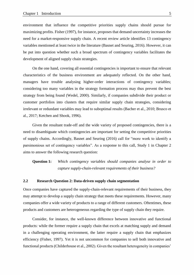
As indicated in Figure 1.1, aligning supply chain strategies with the requirements of the
business environment is a three-step process. First, companies need to gain an understanding
of the environment they operate in. For this purpose, they may gather information on supply-
chain-relevant characteristics of their business. Second, companies need to assess to what extent
the captured requirements diverge across their portfolio of products and customers. If their
products and customers are relatively similar, companies may proceed with the third step and
develop a single supply chain strategy that aligns with the characteristics of their business.
However, if products and customers differ regarding the type of supply chain they require,
companies need to create groups (“segments”) of products or customers with distinct
characteristics. For each segment, companies may then develop a supply chain strategy that fits
the segment-specific requirements. In the following, we highlight gaps in the extant literature
that prevent the execution of these steps and derive corresponding research questions.
Chapter 1 Introduction 4
Figure 1.1: Three-step process for achieving supply chain fit with corresponding literature
gaps and research questions.
2.1 Research Question 1: Capturing requirements of the business environment
The importance of supply chain fit is widely acknowledged and nowadays resonates in
practitioner frameworks and learning materials (APICS, 2016; Gartner, 2016b). Nonetheless,
many companies fail to align their supply chains with the requirements of their business (Gligor,
2015, 2017; Wagner et al., 2012). One likely reason for this seemingly paradoxical observation
is that business environments are complex: managers need to consider many different factors
when setting the competitive priorities of their supply chains.
To help managers decide on supply chain strategies, the extant literature has introduced
a variety of contingency variables. Contingency variables reflect characteristics of the business
Chapter 1 Introduction 5
environment that influence the competitive priorities supply chains should pursue for
maximizing profits. Fisher (1997), for instance, proposes that demand uncertainty increases the
need for a market-responsive supply chain. A recent review article identifies 13 contingency
variables mentioned at least twice in the literature (Basnet and Seuring, 2016). However, it can
be put into question whether such a broad spectrum of contingency variables facilitates the
development of aligned supply chain strategies.
On the one hand, covering all essential contingencies is important to ensure that relevant
characteristics of the business environment are adequately reflected. On the other hand,
managers have trouble analysing higher-order interactions of contingency variables;
considering too many variables in the strategy formation process may thus prevent the best
strategy from being found (Wedel, 2000). Similarly, if companies subdivide their product or
customer portfolios into clusters that require similar supply chain strategies, considering
irrelevant or redundant variables may lead to suboptimal results (Bacher et al., 2010; Brusco et
al., 2017; Ketchen and Shook, 1996).
Given the resultant trade-off and the wide variety of proposed contingencies, there is a
need to disambiguate which contingencies are important for setting the competitive priorities
of supply chains. Accordingly, Basnet and Seuring (2016) call for “more work to identify a
parsimonious set of contingency variables”. As a response to this call, Study 1 in Chapter 2
aims to answer the following research question:
Question 1: Which contingency variables should companies analyse in order to
capture supply-chain-relevant requirements of their business?
2.2 Research Question 2: Data-driven supply chain segmentation
Once companies have captured the supply-chain-relevant requirements of their business, they
may attempt to develop a supply chain strategy that meets these requirements. However, many
companies offer a wide variety of products to a range of different customers. Oftentimes, these
products and customers are heterogeneous regarding the type of supply chain they require.
Consider, for instance, the well-known difference between innovative and functional
products: while the former require a supply chain that excels at matching supply and demand
in a challenging operating environment, the latter require a supply chain that emphasizes
efficiency (Fisher, 1997). Yet it is not uncommon for companies to sell both innovative and
functional products (Childerhouse et al., 2002). Given the resultant heterogeneity in companies’

Chapter 1 Introduction 6
product and customer portfolios, supply chain segmentation has become an emergent practice.
It describes the process of dividing a heterogeneous set of products or customers into groups
(“segments”) that impose similar requirements on the supply chain. For each of these segments,
a tailored supply chain strategy is developed.
Supply chain segmentation, therefore, allows companies to more accurately align their
supply chain capabilities and structures to the requirements of their business. Compared to a
company with a single supply chain strategy, a company with a tailored strategy for each
segment may operate some parts of its business at lower cost and extract higher revenues from
other parts. As a result, supply chain segmentation is considered one of the most effective levers
for improving supply chain performance (Rexhausen et al., 2012) and has been linked to lower
inventories, higher service levels and lower logistics cost (Mayer et al., 2009). A recent survey
by Gartner, a consultancy, concludes that “an overwhelming 95% of [chief supply chain
officers] expect to invest in supply chain segmentation in 2016, with 35% calling it a top
priority” (Gartner, 2016a).
Despite practitioners’ interest in the topic, the number of corresponding studies is limited
so far. A key characteristic of the extant literature on supply chain segmentation is a qualitative
approach to segment formation: segments are formed using managers’ tacit knowledge, without
a systematic data analysis.
This approach has its drawbacks. Managers’ tacit knowledge is subjective; relevant
clusters of products or customers may remain undetected as a result (Foedermayr and
Diamantopoulos, 2008). Especially if product or customer portfolios are broad and
heterogeneous, it is unlikely that managers will have a comprehensive overview of all relevant
segmentation criteria and objects (Wedel, 2000). A supply chain segmentation initiative that
exclusively relies on managers’ tacit knowledge can thus only provide limited insights.
Consequently, authors of segmentation methodologies in marketing urge practitioners to
refrain from solely relying on the qualitative approach (Foedermayr and Diamantopoulos, 2008;
Wedel, 2000). There are many examples of segmentation initiatives in other areas of business
research that employ data analysis to derive segments (Ngai et al., 2009). The supply chain
community, however, appears to be lagging behind in this regard: with one exception
(Langenberg et al., 2012), articles in scholarly journals exclusively rely on managers’ tacit
knowledge for this purpose. Strikingly, the two most commonly employed methods for deriving
segments in other areas of business research – clustering and classification (Ngai et al., 2009)
Chapter 1 Introduction 7
– have not been used in studies on supply chain segmentation so far. Study 2 in Chapter 3
therefore examines how clustering and classification can be used to form supply chain segments
quantitatively. In doing so, the study aims to answer the following research questions:
Question 2a: How can companies use data-driven methods to form supply chain
segments quantitatively?
Question 2b: What insights do these data-driven methods generate relative to
qualitative approaches?
2.3 Research Question 3: Performance outcomes of responsiveness
Study 3 in Chapter 4 aims to provide insights that facilitate the derivation of supply chain
strategies that fit to segment-specific requirements of the business environment. For this
purpose, the study investigates the performance outcomes of responsiveness. In supply chain
management, responsiveness describes the ability of a supply chain to fulfil orders within a
time frame that is acceptable to the customer (Chen et al., 2004; Holweg, 2005). As this ability
is considered critical for competing successfully in the marketplace, setting lead-time-related
targets is imperative when developing supply chain strategies (APICS, 2016).
However, there are two conflicting perspectives regarding the performance outcomes of
responsiveness. On the one hand, studies on the value of shorter lead times argue that
responsiveness entails a cost premium and, hence, purport that responsiveness is primarily
important for innovative products (Blackburn, 2012; de Treville et al., 2014a; de Treville et al.,
2014b). On the other hand, studies on lean management and just-in-time practices assert that
shorter lead times reduce supply-chain-related costs, especially in stable operating
environments that are typical for functional products (Mackelprang and Nair, 2010; Narasimhan
et al., 2006; Shah and Ward, 2003). To determine in which contexts companies should make
responsiveness a competitive priority, we formulate the following research question:
Question 3: When should companies make supply chain responsiveness a competitive
priority?
Empirical basis
3.1 Data requirements
Answering the research questions formulated in the previous section requires two types of data:
archival data from company databases and data on qualitatively derived supply chain segments.
Chapter 1 Introduction 8
The need for archival data from company databases is inherent to all studies in this thesis.
Study 1 aims to provide companies a better understanding as to which characteristics of their
business they should gather information on when developing a supply chain strategy. To ensure
practical relevance, the study focuses its analysis on contingencies that companies can attain
information on without a large data gathering effort, i.e., where data is available in company
databases. Study 2 investigates how companies can use clustering and classification to
subdivide their business into segments that are distinct regarding supply-chain-relevant
characteristics. Consequently, the study requires data on the characteristics of potential
segmentation objects (e.g., products, customers, or business units) from a company that
operates in a broad set of business environments. Finally, Study 3 analyses how different
contextual factors affect the performance outcomes of responsiveness. Since data on
responsiveness (i.e., lead times and customer expectations), performance outcomes (e.g.,
financial performance or supply-chain-related costs) and supply-chain-relevant contingencies
is available in company databases, using archival company data is a natural choice for this study
as well.
In addition, Study 2 requires data on qualitatively derived supply chain segments. The
study investigates how supply chain segments formed with company data compare to segments
formed based on managers’ judgment. For this purpose, it requires not only archival company
data for deriving segments quantitatively, but also information on qualitatively formed
segments.
3.2 Case company
The case company of this thesis is BASF, the largest chemicals company worldwide with
revenues in excess of 50 billion Euros annually (American Chemical Society, 2017). The
company is highly diverse regarding the business environments it operates in, since it embraces
the “Verbund”-concept: BASF controls multiple value streams that span from basic chemicals
to high-value-added products such as coating and crop protection agents (BASF SE, 2016b).
Business units producing basic chemicals, for example, typically operate in stable low-margin
environments. On the contrary, business units producing high-value crop protection or coatings
for the automotive industry operate in volatile high-margin environments.
As a result of its size and diversity, the company fulfils both requirements outlined in the
previous section. First, its broad and diverse portfolio of products and business units provides
this thesis a large sample of archival data with considerable variance. Second, to comprehend
Chapter 1 Introduction 9
the diverse requirements of its business units, BASF has formed a set of supply chain segments
based on managers’ tacit knowledge, hence allowing for a comparison of qualitatively and
quantitatively formed segments.
3.3 Data characteristics
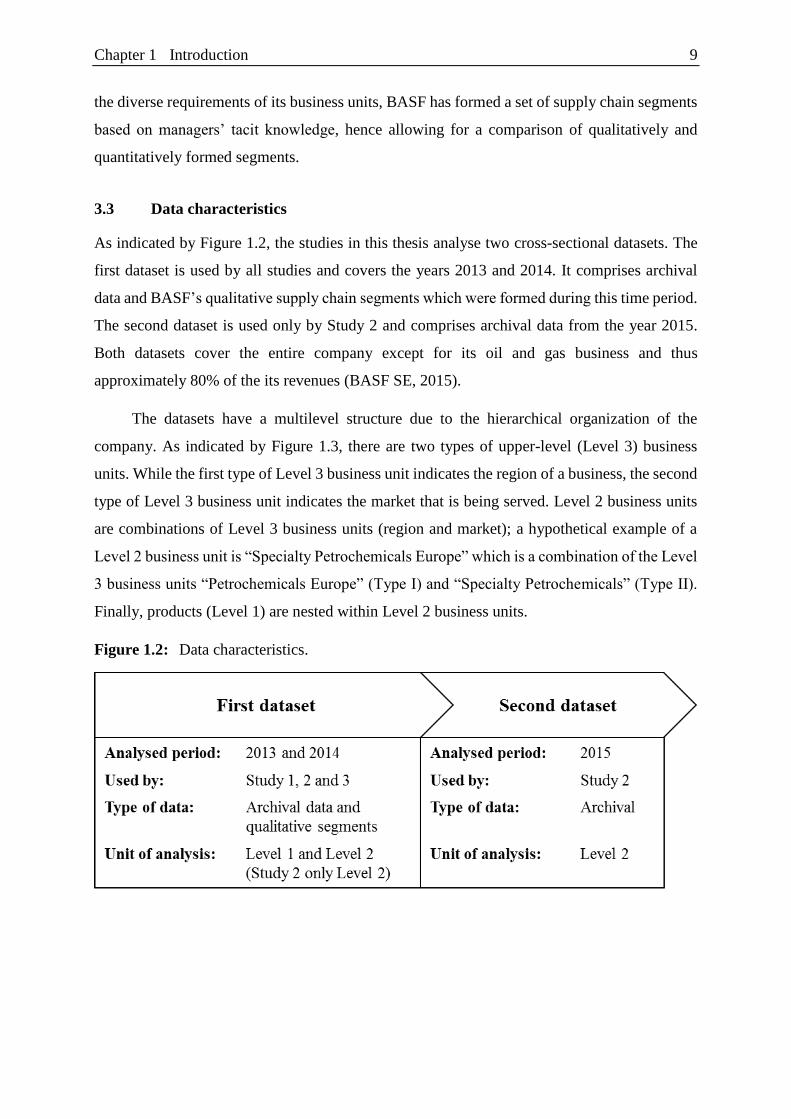
As indicated by Figure 1.2, the studies in this thesis analyse two cross-sectional datasets. The
first dataset is used by all studies and covers the years 2013 and 2014. It comprises archival
data and BASF’s qualitative supply chain segments which were formed during this time period.
The second dataset is used only by Study 2 and comprises archival data from the year 2015.
Both datasets cover the entire company except for its oil and gas business and thus
approximately 80% of the its revenues (BASF SE, 2015).
The datasets have a multilevel structure due to the hierarchical organization of the
company. As indicated by Figure 1.3, there are two types of upper-level (Level 3) business
units. While the first type of Level 3 business unit indicates the region of a business, the second
type of Level 3 business unit indicates the market that is being served. Level 2 business units
are combinations of Level 3 business units (region and market); a hypothetical example of a
Level 2 business unit is “Specialty Petrochemicals Europe” which is a combination of the Level
3 business units “Petrochemicals Europe” (Type I) and “Specialty Petrochemicals” (Type II).
Finally, products (Level 1) are nested within Level 2 business units.
Figure 1.2: Data characteristics.

Chapter 1 Introduction 10
Figure 1.3: Multilevel data structure.
Study 1 and 3 use the first dataset as their empirical basis. The studies focus their analyses
on Level 1 and Level 2, as these levels provide sufficient observations for testing hypothesis.
Study 2 uses data from both datasets. The study focuses its analyses on business units at Level
2 to ensure comparability with BASF’s qualitative supply chain segments which the company
has formed at same level of aggregation. The study employs the first dataset to form segments
with a cluster analysis and to compare the results to BASF’s qualitatively formed segments; the
second dataset is employed to demonstrate how classification algorithms can be used for
updating quantitatively formed segments.
The first dataset comprises 228 observations at Level 2. Some of the business units at that
level have few supply-chain-related activities (e.g., research and design business units). These
business units exhibit extreme values for financial performance (due to low sales) or supply
chain variables (due to few orders). Consequently, the studies in this thesis exclude business
units with annual sales below 1 million Euros or fewer than 1,000 orders annually. In addition,
the studies exclude one business unit that is not reliably integrated into BASF databases and
one business unit with missing financial data. Study 3 further excludes one business unit with
missing data for logistics costs and three business units with extreme values for financial
performance. The final sample of business units from the first dataset located at Level 2
therefore comprises 181 observations for Study 1 and 2, and 177 observations for Study 3.
At Level 1, the dataset comprises 133,687 products that can be uniquely assigned to the
remaining 181 Level 2 business units (132,476 products can be uniquely to the 177 Level 2
business units of Study 3). Following the removal of products with missing data or negative

Chapter 1 Introduction 11
values, the final sample of products comprises 101,071 observations for Study 1 and 77,710
observations for Study 3.
Finally, the second dataset comprises 216 observations at Level 2. Again, we remove all
business units with annual sales below 1 million Euros, fewer than 1,000 orders annually or
missing values. As a result, the final sample of Level 2 business units in the second dataset used
for Study 2 comprises 151 observations.

Chapter 1 Introduction 12
Chapter 2 Contingency variables 13
Chapter 2 Contingency variables for developing supply chain
strategies: An analysis of the DWV3 framework
Co-author:
Moritz Fleischmann
Chair of Logistics and Supply Chain Management, Business School, University of
Mannheim, Germany
Abstract
Contingency variables are characteristics of the business environment that influence the
competitive priorities supply chains should pursue for maximizing profits. But which
contingency variables should managers focus on when developing a supply chain strategy? On
the one hand, if important variables are omitted, the selected strategy may fail to fulfil the needs
of the business environment. On the other hand, considering irrelevant variables unnecessarily
complicates the strategy formation process, hence preventing well-suited strategies from being
found. As a first step towards resolving this trade-off, our study empirically examines the effects
hypothesized to be underlying the five most frequently cited contingency variables in supply
chain strategy literature that are referred to as DWV3 (product lifecycle Duration, customer
lead time requirements / delivery time Window, demand Variability, demand Volume, product
Variety). We test the hypothesis on archival data from a leading chemical manufacturer using
multilevel regression and multilevel structural equation modelling. Our findings indicate that
demand variability and customer lead time requirements are important for strategy development
because they indicate whether companies require market mediation capabilities to fulfil demand
as requested by customers. Volume, variety and lifecycle duration are less important for this
purpose, but may instead be used for analysing the causes of variable demand. Yet, as our study
examines only a subset of the contingencies proposed in the extant literature, additional research
is needed to further disambiguate which contingencies companies should focus on when
developing supply chain strategies.
Chapter 2 Contingency variables 14
Motivation
In the last two decades, a thrust of studies has analysed trade-offs companies face when deciding
on a supply chain strategy (Aitken et al., 2005; Childerhouse et al., 2002; Fisher, 1997; Lee,
2002; Olhager, 2003; Qi et al., 2009; Randall and Ulrich, 2001). Put simply, these studies
conclude that there is no one-size-fits-all supply chain strategy. As a result, the importance of
trade-offs is widely acknowledged and nowadays resonates in practitioner frameworks and
learning materials (APICS, 2016; Gartner, 2016b). However, despite this widespread
awareness, many companies operate supply chains that underserve or overserve the needs of
their business (Gligor, 2015; Wagner et al., 2012). One likely explanation for this seemingly
paradoxical observation is that business environments are complex: managers need to consider
many different factors when setting the competitive priorities of their supply chains.
To help managers decide on supply chain strategies, the extant literature has introduced
a variety of contingency variables. Contingency variables are characteristics of the business
environment that influence the competitive priorities supply chains should pursue for
maximizing profits. Fisher (1997), for instance, proposes that demand uncertainty increases the
need for a market-responsive supply chain. A recent review article identifies 13 contingencies
mentioned at least twice in the literature (Basnet and Seuring, 2016). However, it can be put
into question whether such a broad spectrum of contingency variables is helpful to managers.
On the one hand, covering all essential contingencies is important to ensure that relevant
characteristics of the business environment are adequately reflected. On the other hand,
however, managers have trouble analysing higher-order interactions of contingency variables;
considering too many variables in the strategy formation process may thus prevent the best
strategy from being found (Wedel, 2000). Similarly, if companies subdivide their product or
customer portfolios into clusters that require similar supply chain strategies, considering
irrelevant or redundant variables may lead to suboptimal results (Bacher et al., 2010; Brusco et
al., 2017; Ketchen and Shook, 1996). Consequently, there is a “need for more work to identify
a parsimonious set of contingency variables” (Basnet and Seuring, 2016).
An established practice in marketing strategy for obtaining a parsimonious set of
contingencies is to empirically examine the effects that are assumed to be underlying the
variables of interest. Cooil et al. (2007) and Wangenheim and Bayon (2004), for instance,
examine the relevance of different customer characteristics for tailoring marketing actions by
testing whether they are significant moderators of the link between customer satisfaction and
loyalty. However, we are not aware of any studies that empirically examine the effects
Chapter 2 Contingency variables 15
hypothesized to be underlying contingencies that are potentially important for developing
supply chain strategies. As a first step towards filling this gap, our study examines the effects
of the five most frequently cited contingency variables in literature on supply chain strategy
that are referred to as DWV3 (product lifecycle Duration, customer lead time requirement /
delivery time Window, demand Variability, demand Volume, product Variety) (Christopher et
al., 2009). Specifically, we use archival data from the chemicals company BASF to test to what
extent the DWV3 variables necessitate investments in market mediation for demand to be
fulfilled as requested by customers. In doing so, our study contributes by taking a first step
towards disambiguating which contingencies are important for setting the competitive priorities
of supply chains.1
The remainder of this article proceeds as follows. Section 2 provides an overview of the
contingency variables proposed in the extant literature by grouping together contingencies with
similar effects. Section 3 introduces the variables examined as part of our study. Section 4
provides further theoretical background for deriving hypothesis. Section 5 outlines the dataset
and specifies the measures used. Section 6 introduces the methodology. The results of our
analysis are outlined in Section 7 and discussed in Section 8. Section 9 derives implications and
concludes with the limitations of our work and suggestions for future research.
Categorizing contingency variables
Supply chains have two distinct functions: the physical function and the market mediation
function (Fisher, 1997). The former minimizes the costs of supply-chain-related activities such
as production, distribution and warehousing. The latter ensures the reliable fulfilment of
demand according to customer specification in order to avoid lost sales. Two types of
contingency variables influence the relative importance of these functions.
Challenges in the operating environment are contingencies that make it harder to fulfil
demand as requested by customers, ceteris paribus. In a stable environment with few
uncertainties, supply chains may adopt practices that allow reliable operations at low costs
(Azadegan et al., 2013; Browning and Heath, 2009). However, in environments characterized
by uncertainty and time pressure, supply chains require market mediation capabilities such as
responsiveness, flexibility or agility in order to fulfil demand according to customer
specifications (de Treville et al., 2014a; Gligor et al., 2015; Wagner et al., 2012). Since many
1 Further research is needed in this regard, since the DWV3 variables comprise only five of thirteen contingencies
identified as potentially relevant for developing supply chain strategies by Basnet and Seuring (2016).

Chapter 2 Contingency variables 16
measures that facilitate market mediation are costly, challenges in the operating environment
therefore indicate whether there is a trade-off between efficiency and market mediation
(Randall and Ulrich, 2001).
The second type of contingency variables influences the value of market mediation. Even
though investments in market mediation capabilities are a prerequisite for reliably fulfilling
demand in a challenging operating environment, this does not imply that such investments
should necessarily be taken: companies need to ensure that the financial reward of better
fulfilling demand clearly outweigh the associated costs. Hence, when deciding whether or not
to invest in market mediation in a challenging operating environment, companies may need to
consider contingencies influencing the effect of lost sales on the bottom line.
In the following, we outline challenges in the operating environment and contingencies
affecting the value of market mediation that have been proposed in the extant literature.
2.1 Challenges in the operating environment
By making it harder to reliably fulfil demand, ceteris paribus, contingencies of this type
influence to what extent companies require market mediation capabilities to avoid lost sales.
As indicated by Table 2.1, challenges in the operating environment can be categorized as
demand-related, time-related and supply-related.
Chapter 2 Contingency variables 17
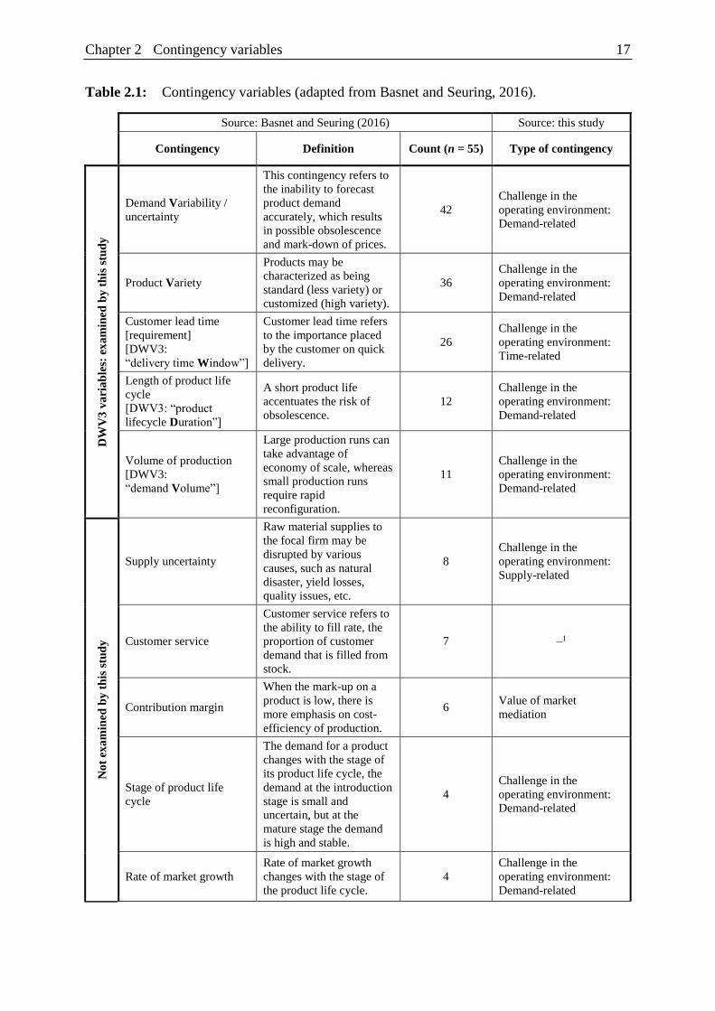
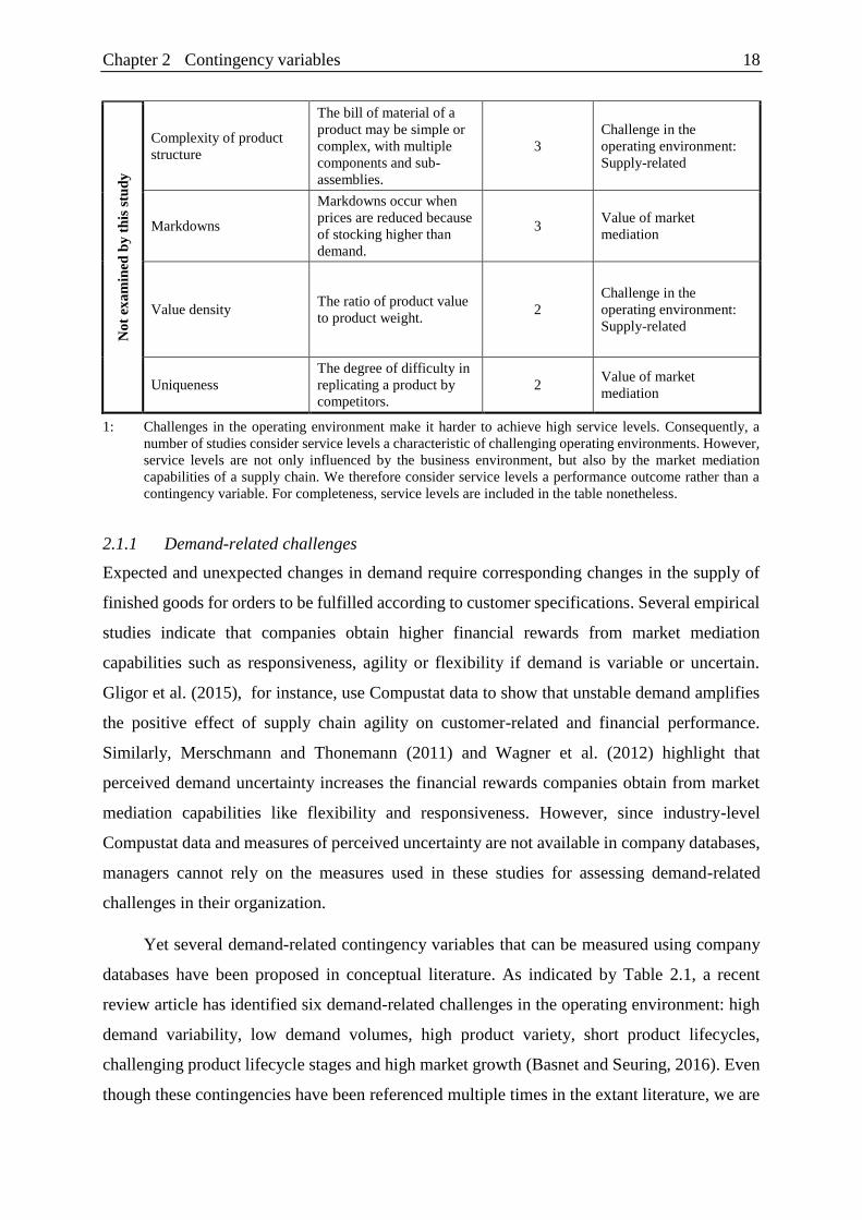
Table 2.1: Contingency variables (adapted from Basnet and Seuring, 2016).
Source: Basnet and Seuring (2016) Source: this study
Contingency Definition Count (n = 55) Type of contingency
DW
V3
va
ria
ble
s: e
xa
min
ed b
y t
his
stu
dy
Demand Variability /
uncertainty
This contingency refers to
the inability to forecast
product demand
accurately, which results
in possible obsolescence
and mark-down of prices.
42
Challenge in the
operating environment:
Demand-related
Product Variety
Products may be
characterized as being
standard (less variety) or
customized (high variety).
36
Challenge in the
operating environment:
Demand-related
Customer lead time
[requirement]
[DWV3:
“delivery time Window”]
Customer lead time refers
to the importance placed
by the customer on quick
delivery.
26
Challenge in the
operating environment:
Time-related
Length of product life
cycle
[DWV3: “product
lifecycle Duration”]
A short product life
accentuates the risk of
obsolescence.
12
Challenge in the
operating environment:
Demand-related
Volume of production
[DWV3:
“demand Volume”]
Large production runs can
take advantage of
economy of scale, whereas
small production runs
require rapid
reconfiguration.
11
Challenge in the
operating environment:
Demand-related
No
t ex
am
ined
by
th
is s
tud
y
Supply uncertainty
Raw material supplies to
the focal firm may be
disrupted by various
causes, such as natural
disaster, yield losses,
quality issues, etc.
8
Challenge in the
operating environment:
Supply-related
Customer service
Customer service refers to
the ability to fill rate, the
proportion of customer
demand that is filled from
stock.
7 –1
Contribution margin
When the mark-up on a
product is low, there is
more emphasis on cost-
efficiency of production.
6 Value of market
mediation
Stage of product life
cycle
The demand for a product
changes with the stage of
its product life cycle, the
demand at the introduction
stage is small and
uncertain, but at the
mature stage the demand
is high and stable.
4
Challenge in the
operating environment:
Demand-related
Rate of market growth
Rate of market growth
changes with the stage of
the product life cycle.
4
Challenge in the
operating environment:
Demand-related
Chapter 2 Contingency variables 18
No
t ex
am
ined
by
th
is s
tud
y
Complexity of product
structure
The bill of material of a
product may be simple or
complex, with multiple
components and sub-
assemblies.
3
Challenge in the
operating environment:
Supply-related
Markdowns
Markdowns occur when
prices are reduced because
of stocking higher than
demand.
3 Value of market
mediation
Value density The ratio of product value
to product weight. 2
Challenge in the
operating environment:
Supply-related
Uniqueness
The degree of difficulty in
replicating a product by
competitors.
2 Value of market
mediation
1: Challenges in the operating environment make it harder to achieve high service levels. Consequently, a
number of studies consider service levels a characteristic of challenging operating environments. However,
service levels are not only influenced by the business environment, but also by the market mediation
capabilities of a supply chain. We therefore consider service levels a performance outcome rather than a
contingency variable. For completeness, service levels are included in the table nonetheless.
2.1.1 Demand-related challenges
Expected and unexpected changes in demand require corresponding changes in the supply of
finished goods for orders to be fulfilled according to customer specifications. Several empirical
studies indicate that companies obtain higher financial rewards from market mediation
capabilities such as responsiveness, agility or flexibility if demand is variable or uncertain.
Gligor et al. (2015), for instance, use Compustat data to show that unstable demand amplifies
the positive effect of supply chain agility on customer-related and financial performance.
Similarly, Merschmann and Thonemann (2011) and Wagner et al. (2012) highlight that
perceived demand uncertainty increases the financial rewards companies obtain from market
mediation capabilities like flexibility and responsiveness. However, since industry-level
Compustat data and measures of perceived uncertainty are not available in company databases,
managers cannot rely on the measures used in these studies for assessing demand-related
challenges in their organization.
Yet several demand-related contingency variables that can be measured using company
databases have been proposed in conceptual literature. As indicated by Table 2.1, a recent
review article has identified six demand-related challenges in the operating environment: high
demand variability, low demand volumes, high product variety, short product lifecycles,
challenging product lifecycle stages and high market growth (Basnet and Seuring, 2016). Even
though these contingencies have been referenced multiple times in the extant literature, we are

Chapter 2 Contingency variables 19
not aware of any studies that empirically test whether they significantly affect the ability to
fulfil demand as requested by customers. Consequently, it remains unclear which of these
variables should be considered in the strategy development process.
2.1.2 Time-related challenges
Reliably fulfilling demand is also more difficult if customers require off-the-shelf availability
or quick delivery. The shorter the period between order placement and requested delivery date,
the less time is available for reacting to unexpected changes in demand. The emphasis
customers place on short-notice delivery is therefore considered a critical contingency for
strategic decisions such as selecting sourcing locations (de Treville et al., 2014a), setting the
decoupling point (Olhager, 2003) and deciding on a transportation mode (Verma and Verter,
2010).
The measurement of time-related challenges depends on the supply chain design decision
in question. The ratio between lead times accepted by the customer and the production lead
time indicates whether make-to-order production is feasible (Olhager, 2003). The customer lead
time requirement – i.e., the time between order placement and requested delivery – is
considered a key determinant for valuing lead times in sourcing decisions (de Treville et al.,
2014a) and when choosing transportation modes (Verma and Verter, 2010). The authors of the
DWV3 framework, whilst referring to the customer lead time requirement as the “delivery time
window”, concur that lead time requirements are important for deciding on supply chain
strategies (Christopher et al., 2009).2 However, similar to the introduced demand-related
challenges, we are not aware of any studies that empirically test whether the proposed time-
related challenges significantly affect the ability to fulfil demand as requested by customers.
2.1.3 Supply-related challenges
The fulfilment of demand may also be disrupted by unexpected changes in the ability to provide
finished goods to customers. Supply-related challenges in the operating environment increase
the likelihood of disruptions in source, make or deliver processes.
Disruptions in the supply of critical materials starve the production and thus prevent the
fulfilment of customer demand. Contingencies affecting the likelihood of disruptions in the
supply of materials relate to supplier performance (e.g., variance of material supply lead time),
2 Contrary to the DWV3 framework, we will henceforth refer to the time between order placement and requested
delivery date as the “customer lead time requirement”. We thereby aim to emphasize that customers’ preferences
regarding lead times impose requirements on supply chains that are potentially important for developing supply
chain strategies.
Chapter 2 Contingency variables 20
substitutability of suppliers (e.g., number of critical material suppliers) or material criticality
(e.g., time-specificity of materials) (Ho et al., 2005).
Further, disruptions in manufacturing may prevent customer demand from being fulfilled
as well. Contingencies affecting the likelihood of disruptions in the production of finished
goods relate to product complexity (e.g., product modularity), the degree of process interaction
(e.g., degree of pre-process output on post-process performance) or product redesigns (e.g.,
frequency of redesigns) (Ho et al., 2005).
Finally, there are contingencies that make the delivery of finished goods more
challenging. Low product value density (i.e., low value products with high weight) renders the
usage of fast transportation modes prohibitively expensive (Lovell et al., 2005). Similarly,
difficult terrain and unreliable transportation infrastructure increase the likelihood of
disruptions in transportation (Simangunsong et al., 2012).
However, there is little research examining the effects of supply-related challenges in the
operating environment. Ho et al. (2005) highlight that companies facing supply-related
challenges are more likely to invest in supply chain flexibility. Yet to what extent variables of
this type affect the ability to fulfil demand as requested by customers has not been empirically
analysed so far.
2.2 Value of market mediation
In challenging operating environments, market mediation capabilities generate additional sales
by preventing shortages. However, preventing lost sales comes at the expense of lower physical
efficiency, since many capabilities that facilitate market mediation are costly (Randall and
Ulrich, 2001). To evaluate whether the financial reward of preventing shortages outweighs the
cost of market mediation, managers may therefore need to consider contingencies that affect
the value of fulfilling demand more reliably when developing supply chain strategies.
The most frequently-cited contingency of this category is the contribution margin.
Contribution margins are a key determinant of the value of market mediation because they
influence the effect of lost sales on the bottom line (Randall et al., 2003). If contribution margins
are high, managers should be willing to incur higher market mediation costs, since the cost of
lost sales is also higher (Hendricks and Singhal, 2003). However, other variables are potentially
important for determining value of market mediation as well. Contract penalties and goodwill
Chapter 2 Contingency variables 21
loss in case of late delivery, for instance, may also incentivize companies to invest in market
mediation by increasing the cost of shortages (Langenberg et al., 2012).
Focus of this study: DWV3 variables
The previous chapter highlights that (1) there is a broad spectrum of potentially relevant
contingency variables, (2) these variables are hypothesized to affect the relative importance of
competitive priorities in different ways, yet (3) these hypothesized effects have not been
empirically validated so far. As a result, companies are confronted with a wide variety of
potentially relevant contingency variables, but with little guidance as to which of these variables
they should take into consideration when developing supply chain strategies. Our study
therefore takes a first step towards disambiguating which contingencies companies need to
consider for this purpose by testing the effects hypothesized to be underlying a set of variables
that has been termed DWV3: product lifecycle Duration, customer lead time requirement
(delivery time Window), demand Variability, demand Volume, product Variety (Christopher
et al., 2009).
We restrict our analysis to the DWV3 variables, since supply chain strategy literature
perpetuates that these variables are the most important contingencies. Aitken et al. (2005), for
example, refer to the DWV3 variables as the “five key […] characteristics that should influence
decision making”. Christopher et al. (2009) devote an entire article to the DWV3 variables,
stating that they are the “five key characteristics that influence decision making on the design
of value stream delivery strategies”. In line with these statements, Table 2.1 indicates that the
DWV3 variables are by far the most frequently cited contingency variables. The DWV3
variables are thus a natural starting point for both practitioners and researchers enquiring which
contingencies need to be taken into consideration when setting the competitive priorities of
supply chains.
Nonetheless, this study constitutes only a first step towards disambiguating which
contingencies are important for setting competitive priorities, as the DWV3 variables comprise
solely demand-related and time-related challenges in the operating environment. Yet two other
types of variables are potentially relevant as well. First, supply-related challenges in the
operating environment may necessitate higher investments in the market mediation than
indicated by the DWV3 variables for demand to be fulfilled reliably. Second, variables
influencing the effect of lost sales on the bottom line might be important for determining
whether the financial rewards of better fulfilling demand outweigh the associated costs.
Chapter 2 Contingency variables 22
Consequently, in order to provide companies a parsimonious set of contingencies that conveys
a holistic picture of the business environment, further research needs to investigate the effects
of these two types of variables.
Hypothesis development
4.1 Conceptual framework
The DWV3 variables reflect challenges in the operating environment. Hence, we expect these
variables to (1) make it harder to fulfil demand as requested by customers, ceteris paribus, and
(2) increase the financial rewards companies can obtain from market mediation capabilities, as
there are more opportunities for reducing lost sales when it is hard to fulfil demand as requested.
Consequently, there are two possible approaches for evaluating whether the DWV3
variables necessitate investments in market mediation. First, we may test to what extent the
DWV3 variables reduce the ability of companies to fulfil demand as requested by customers,
ceteris paribus. Second, we may test to what extent the DWV3 variables increase the financial
rewards companies can obtain from market mediation capabilities.
Empirical articles in the extant literature have largely opted for the second modelling
approach. These articles examine how uncertainty-related contingencies affect the link between
individual market mediation capabilities and financial performance. Gligor et al. (2015), for
example, highlight that the positive effect of supply chain agility on financial performance
increases with different types of environmental uncertainty. Merschmann and Thonemann
(2011) present similar findings for supply chain flexibility. However, while this approach is
feasible for individual market mediation capabilities, it is less suitable for examining how
contingencies affect the performance outcomes of market mediation capabilities in general, as
it is not sufficiently clear which capabilities one would have to evaluate for this purpose (Basnet
and Seuring, 2016). Proposed market mediation capabilities range from different aspects of
responsiveness (e.g., Bernardes and Hanna, 2009), agility (e.g., Gligor et al., 2013), flexibility
(e.g., Swafford et al., 2006) to different sources of resilience (e.g., Pettit et al., 2010). Given the
resultant ambiguity as to which capabilities are important for market mediation and how these
capabilities should be operationalized, we have opted for the first modelling approach described
in the previous paragraph. Specifically, our study tests the direct and indirect effects of the
DWV3 variables on the ability of supply chains to fulfil demand according to customer
specifications.
Chapter 2 Contingency variables 23
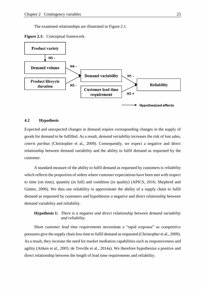
The examined relationships are illustrated in Figure 2.1.
Figure 2.1: Conceptual framework.
4.2 Hypothesis
Expected and unexpected changes in demand require corresponding changes in the supply of
goods for demand to be fulfilled. As a result, demand variability increases the risk of lost sales,
ceteris paribus (Christopher et al., 2009). Consequently, we expect a negative and direct
relationship between demand variability and the ability to fulfil demand as requested by the
customer.
A standard measure of the ability to fulfil demand as requested by customers is reliability
which reflects the proportion of orders where customer expectations have been met with respect
to time (on time), quantity (in full) and condition (in quality) (APICS, 2016; Shepherd and
Günter, 2006). We thus use reliability to approximate the ability of a supply chain to fulfil
demand as requested by customers and hypothesize a negative and direct relationship between
demand variability and reliability.
Hypothesis 1: There is a negative and direct relationship between demand variability
and reliability.
Short customer lead time requirements necessitate a “rapid response” as competitive
pressures give the supply chain less time to fulfil demand as requested (Christopher et al., 2009).
As a result, they increase the need for market mediation capabilities such as responsiveness and
agility (Aitken et al., 2005; de Treville et al., 2014a). We therefore hypothesize a positive and
direct relationship between the length of lead time requirements and reliability.
Chapter 2 Contingency variables 24
Hypothesis 2: There is a positive and direct relationship between the length of customer
lead time requirements and reliability.
As indicated by Table 2.1, the extant literature also considers the remaining DWV3
variables important for determining whether companies require market mediation capabilities
to reliably fulfil demand. One might thus be inclined to hypothesize a direct relationship
between the remaining DWV3 variables and reliability as well. However, upon closer
examination, it becomes clear that “small production volumes, short product life, large product
variety, all add to the variability of product demand” (Basnet and Seuring, 2016). Consequently,
we expect these variables to affect reliability indirectly by increasing the demand variability.
Products with short lifecycles require supply chains that are “able to ‘fast track’ […]
manufacturing and logistics” (Christopher et al., 2009). The underlying reason is that they spend
relatively large shares of their lives in the introduction and growth stages where demand is
variable and uncertain (Childerhouse et al., 2002). Consequently, we expect short lifecycles to
reduce reliability indirectly by increasing demand variability, ceteris paribus. Accordingly, we
hypothesize a direct relationship between product lifecycle duration and demand variability. In
addition, we analyse whether this relationship also leads to an indirect effect on reliability.
Hypothesis 3: There is a negative and direct relationship between product lifecycle
duration and demand variability.
Low volume products are more likely to have demand that is sporadic and uncertain. Vice
versa, high volume products more often allow make-to-forecast production, as demand tends to
be more stable (Christopher et al., 2009; Zotteri and Kalchschmidt, 2007). Consequently, we
expect higher demand volumes to increase reliability by reducing demand variability, ceteris
paribus. Accordingly, we hypothesize a direct relationship between demand volume and
demand variability. In addition, we analyse whether this relationship also leads to an indirect
effect on reliability.
Hypothesis 4: There is a negative and direct relationship between demand volume and
demand variability.
Regarding product variety, the authors of the DWV3 framework state that “greater variety
results in a larger number of stock keeping units because the volume is split between
alternatives” (Christopher et al., 2009). We therefore expect product variety to decrease
reliability by reducing the volume per product which we in turn expect to increase demand
variability, ceteris paribus. Accordingly, we hypothesize a direct relationship between variety
Chapter 2 Contingency variables 25
and volume. In addition, we analyse whether this relationship also leads to indirect effects on
demand variability and reliability.
Hypothesis 5: There is a negative and direct relationship between product variety and
demand volume.
Dataset
5.1 Data collection and sampling
This study is conducted in cooperation with BASF, one of the world’s leading chemicals
manufacturers. The company is a well-suited subject for our investigation because it embraces
the “Verbund”-concept: the company controls multiple value streams that span from basic
chemicals to high-value-added products such as coatings and crop protection agents (BASF SE,
2016b). As a result, supply-chain-relevant characteristics of the business environment differ
considerably across the company. Business units producing basic chemicals, for example,
typically operate in stable low-margin environments. On the contrary, business units producing
high-value crop protection or coatings for the automotive industry operate in volatile high-
margin environments. Given the resultant diversity of BASF’s portfolio of products and
business units, we consider it plausible that our dataset provides sufficient variance in the
examined contingency variables to warrant the generalization of our findings.
To align the competitive priorities of its supply chains with the diverse requirements of
its business unit portfolio, BASF launched a supply chain segmentation initiative in the years
2013 and 2014: business units were assigned to a set of four segments, each with a distinct
supply chain strategy (Cecere, 2017). As part of the initiative, BASF commissioned this
research project to examine which contingency variables should be considered when assigning
business units to segments. Accordingly, our study is based on a dataset from the 2013 and
2014 that covers the entire company except for its Oil&Gas business, hence capturing
approximately 80% of its revenues (BASF SE, 2015).
The data has a multilevel structure due to the hierarchical organization of the company.
Figure 2.2 indicates that there are two types of upper-level (Level 3) business units. While the
first type of Level 3 business unit indicates the region of a business, the second type of Level 3
business unit indicates the market that is being served. Level 2 business units are combinations
of Level 3 business units (region and market); a hypothetical example of a Level 2 business
unit is “Specialty Petrochemicals Europe” which is a combination of the Level 3 business units
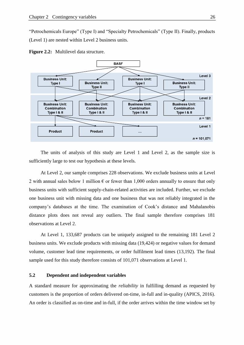
Chapter 2 Contingency variables 26
“Petrochemicals Europe” (Type I) and “Specialty Petrochemicals” (Type II). Finally, products
(Level 1) are nested within Level 2 business units.
Figure 2.2: Multilevel data structure.
The units of analysis of this study are Level 1 and Level 2, as the sample size is
sufficiently large to test our hypothesis at these levels.
At Level 2, our sample comprises 228 observations. We exclude business units at Level
2 with annual sales below 1 million € or fewer than 1,000 orders annually to ensure that only
business units with sufficient supply-chain-related activities are included. Further, we exclude
one business unit with missing data and one business that was not reliably integrated in the
company’s databases at the time. The examination of Cook’s distance and Mahalanobis
distance plots does not reveal any outliers. The final sample therefore comprises 181
observations at Level 2.
At Level 1, 133,687 products can be uniquely assigned to the remaining 181 Level 2
business units. We exclude products with missing data (19,424) or negative values for demand
volume, customer lead time requirements, or order fulfilment lead times (13,192). The final
sample used for this study therefore consists of 101,071 observations at Level 1.
5.2 Dependent and independent variables
A standard measure for approximating the reliability in fulfilling demand as requested by
customers is the proportion of orders delivered on-time, in-full and in-quality (APICS, 2016).
An order is classified as on-time and in-full, if the order arrives within the time window set by
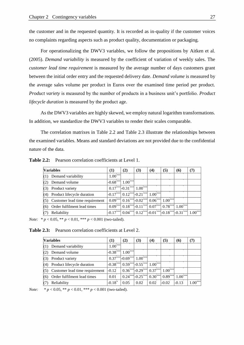
Chapter 2 Contingency variables 27
the customer and in the requested quantity. It is recorded as in-quality if the customer voices
no complaints regarding aspects such as product quality, documentation or packaging.
For operationalizing the DWV3 variables, we follow the propositions by Aitken et al.
(2005). Demand variability is measured by the coefficient of variation of weekly sales. The
customer lead time requirement is measured by the average number of days customers grant
between the initial order entry and the requested delivery date. Demand volume is measured by
the average sales volume per product in Euros over the examined time period per product.
Product variety is measured by the number of products in a business unit’s portfolio. Product
lifecycle duration is measured by the product age.
As the DWV3 variables are highly skewed, we employ natural logarithm transformations.
In addition, we standardize the DWV3 variables to render their scales comparable.
The correlation matrixes in Table 2.2 and Table 2.3 illustrate the relationships between
the examined variables. Means and standard deviations are not provided due to the confidential
nature of the data.
Table 2.2: Pearson correlation coefficients at Level 1.
Variables (1) (2) (3) (4) (5) (6) (7)
(1) Demand variability 1.00 ***
(2) Demand volume -0.68 *** 1.00 ***
(3) Product variety 0.17 *** -0.31 *** 1.00 ***
(4) Product lifecycle duration -0.17 *** 0.12 *** -0.21 *** 1.00 ***
(5) Customer lead time requirement 0.09 *** 0.16 *** -0.02 *** 0.06 *** 1.00 ***
(6) Order fulfilment lead times 0.09 *** 0.18 *** -0.11 *** 0.07 *** 0.78 *** 1.00 ***
(7) Reliability -0.17 *** 0.04 *** 0.12 *** -0.01 *** -0.18 *** -0.31 *** 1.00 ***
Note: * p < 0.05, ** p < 0.01, *** p < 0.001 (two-tailed).
Table 2.3: Pearson correlation coefficients at Level 2.
Variables (1) (2) (3) (4) (5) (6) (7)
(1) Demand variability 1.00 ***
(2) Demand volume -0.38 *** 1.00 ***
(3) Product variety 0.37 *** -0.69 *** 1.00 ***
(4) Product lifecycle duration -0.38 *** 0.59 *** -0.55 *** 1.00 ***
(5) Customer lead time requirement -0.12 0.36 *** -0.29 *** 0.37 *** 1.00 ***
(6) Order fulfilment lead times 0.01 0.24 *** -0.25 *** 0.30 *** 0.89 *** 1.00 ***
(7) Reliability -0.18 * 0.05 0.02 0.02 -0.02 -0.13 1.00 ***
Note: * p < 0.05, ** p < 0.01, *** p < 0.001 (two-tailed).
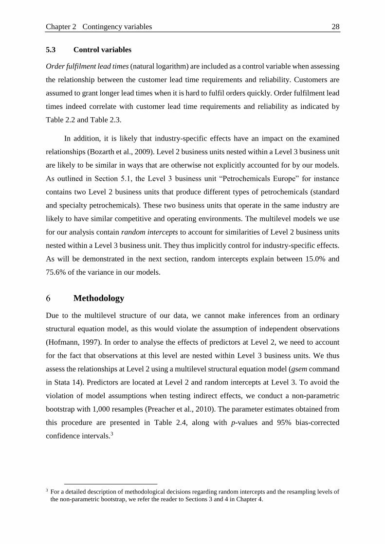
Chapter 2 Contingency variables 28
5.3 Control variables
Order fulfilment lead times (natural logarithm) are included as a control variable when assessing
the relationship between the customer lead time requirements and reliability. Customers are
assumed to grant longer lead times when it is hard to fulfil orders quickly. Order fulfilment lead
times indeed correlate with customer lead time requirements and reliability as indicated by
Table 2.2 and Table 2.3.
In addition, it is likely that industry-specific effects have an impact on the examined
relationships (Bozarth et al., 2009). Level 2 business units nested within a Level 3 business unit
are likely to be similar in ways that are otherwise not explicitly accounted for by our models.
As outlined in Section 5.1, the Level 3 business unit “Petrochemicals Europe” for instance
contains two Level 2 business units that produce different types of petrochemicals (standard
and specialty petrochemicals). These two business units that operate in the same industry are
likely to have similar competitive and operating environments. The multilevel models we use
for our analysis contain random intercepts to account for similarities of Level 2 business units
nested within a Level 3 business unit. They thus implicitly control for industry-specific effects.
As will be demonstrated in the next section, random intercepts explain between 15.0% and
75.6% of the variance in our models.
Methodology
Due to the multilevel structure of our data, we cannot make inferences from an ordinary
structural equation model, as this would violate the assumption of independent observations
(Hofmann, 1997). In order to analyse the effects of predictors at Level 2, we need to account
for the fact that observations at this level are nested within Level 3 business units. We thus
assess the relationships at Level 2 using a multilevel structural equation model (gsem command
in Stata 14). Predictors are located at Level 2 and random intercepts at Level 3. To avoid the
violation of model assumptions when testing indirect effects, we conduct a non-parametric
bootstrap with 1,000 resamples (Preacher et al., 2010). The parameter estimates obtained from
this procedure are presented in Table 2.4, along with p-values and 95% bias-corrected
confidence intervals.3
3 For a detailed description of methodological decisions regarding random intercepts and the resampling levels of
the non-parametric bootstrap, we refer the reader to Sections 3 and 4 in Chapter 4.
Chapter 2 Contingency variables 29
At Level 1, we test the hypothesized effects using a set of multilevel regressions (mixed
command in Stata 14), as the sample size is too large for solving a multilevel structural equation
model. Predictors are located at Level 1 and random intercepts at Level 2 and Level 3.
The results of the regression with reliability as the dependent variable are heteroskedastic.
The heteroscedasticity is caused by the high proportion of products with a reliability of 0% or
100%; most of these products were ordered only a few times during the time period under
consideration. Since they are more likely to exhibit extreme values for reliability (a product that
was only sold once by default has a value for reliability of either 0% or 100%), their values for
reliability are distributed differently from those of the rest of the sample (Cook et al., 2008).
Zero-or-one inflated beta regression models could serve as a remedy, since they assume that
the response variable has a mixed continuous–discrete distribution with probability mass at zero
or one (Ospina and Ferrari, 2012). However, beta regressions are not yet available for multilevel
models. To be able to draw inferences nonetheless, we conduct non-parametric bootstraps with
1,000 resamples for the regressions at Level 1, as standard errors obtained from non-parametric
bootstrapping are still consistent under heteroscedasticity (Godfrey, 2009; van der Leeden et
al., 2008). The indirect effects are tested with Monte Carlo simulations using the results of the
bootstrapping as input (Selig and Preacher, 2008). The results of these procedures are presented
in Table 2.5.
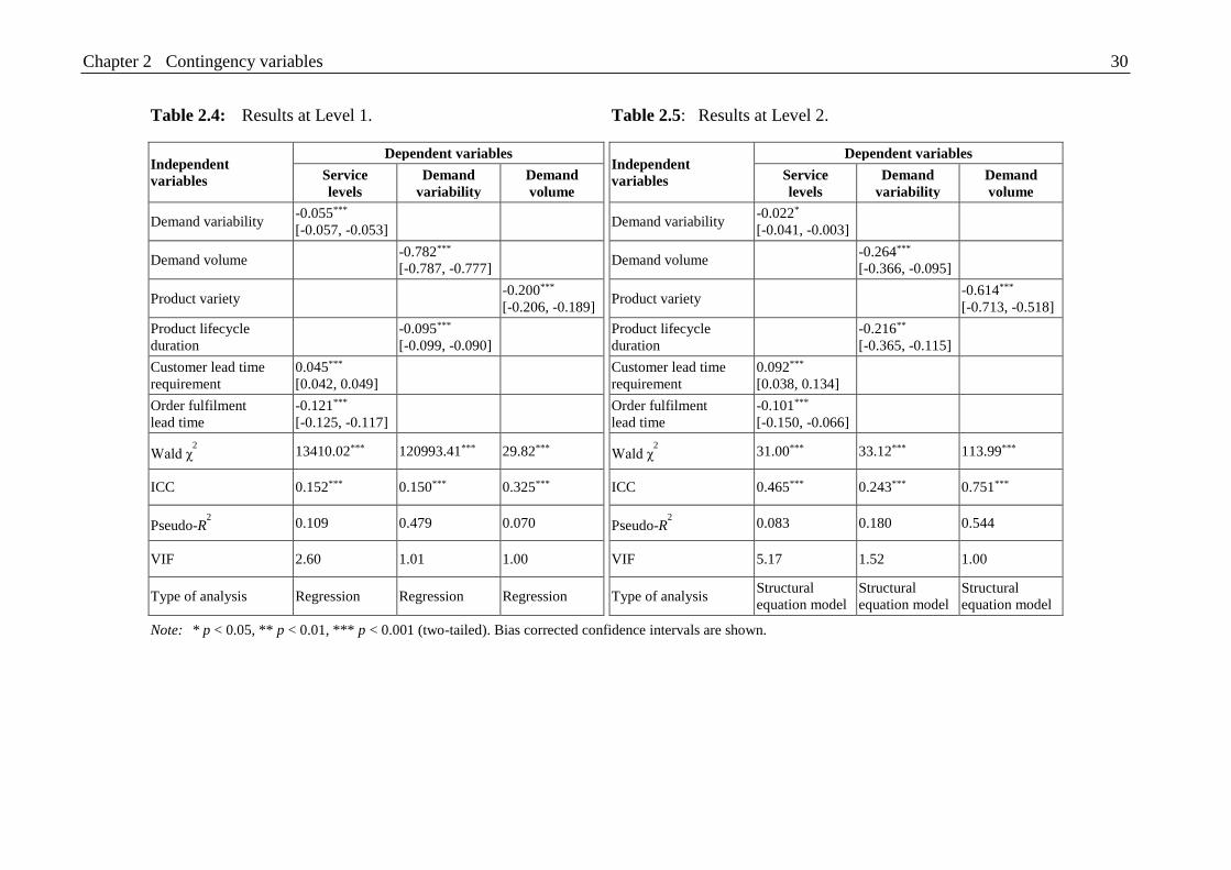
Chapter 2 Contingency variables 30
Table 2.4: Results at Level 1. Table 2.5: Results at Level 2.
Independent
variables
Dependent variables Independent
variables
Dependent variables
Service
levels
Demand
variability
Demand
volume
Service
levels
Demand
variability
Demand
volume
Demand variability -0.055***
[-0.057, -0.053]
Demand variability
-0.022*
[-0.041, -0.003]
Demand volume -0.782***
[-0.787, -0.777]
Demand volume
-0.264***
[-0.366, -0.095]
Product variety -0.200***
[-0.206, -0.189]
Product variety
-0.614***
[-0.713, -0.518]
Product lifecycle
duration -0.095***
[-0.099, -0.090]
Product lifecycle
duration
-0.216**
[-0.365, -0.115]
Customer lead time
requirement
0.045***
[0.042, 0.049]
Customer lead time
requirement
0.092***
[0.038, 0.134]
Order fulfilment
lead time
-0.121***
[-0.125, -0.117]
Order fulfilment
lead time
-0.101***
[-0.150, -0.066]
Wald χ2 13410.02*** 120993.41*** 29.82***
Wald χ
2 31.00*** 33.12*** 113.99***
ICC 0.152*** 0.150*** 0.325*** ICC 0.465*** 0.243*** 0.751***
Pseudo-R2 0.109 0.479 0.070
Pseudo-R
2 0.083 0.180 0.544
VIF 2.60 1.01 1.00 VIF 5.17 1.52 1.00
Type of analysis Regression Regression Regression Type of analysis
Structural
equation model
Structural
equation model
Structural
equation model
Note: * p < 0.05, ** p < 0.01, *** p < 0.001 (two-tailed). Bias corrected confidence intervals are shown.
Chapter 2 Contingency variables 31
Results
Multicollinearity is unlikely to be an issue, as the variance inflation factor (VIF) is within a
tolerable range (maximum VIF = 5.17). The residuals of the model at Level 2 are approximately
normally distributed and homoscedastic. The residuals of the regression at Level 1 are also
approximately normally distributed. For the regression with reliability as the dependent
variable, the residuals are, as expected, heteroskedastic. The intraclass correlation coefficients
(ICC) in Table 2.4 and Table 2.5 indicate that the random intercepts explain a significant
proportion of the variance in our models. At Level 2, the ICC is 0.465 for reliability, 0.243 for
demand variability and 0.751 for demand volume. At Level 1, the ICC is 0.150 for reliability,
0.148 for demand variability and 0.321 for demand volume.4
To assess the level of variance explained by the predictors, we compute a Pseudo-R2
measure for the change in the total variance explained at all levels with and without the
predictors (LaHuis et al., 2014). For the model at Level 2, Table 2.4 indicates that the predictors
explain a significant proportion of the variance in reliability (Pseudo-R2 = 0.083 and Wald χ2 =
31.00, p < 0.001), demand variability (Pseudo-R2 = 0.180 and Wald χ2 = 33.12, p < 0.001) and
demand volume (Pseudo-R2 = 0.544 and Wald χ2 = 113.99, p < 0.001). For the regressions at
Level 1, Table 2.5 also indicates that the predictors explain a significant proportion of the
variance in reliability (Pseudo-R2 = 0.109 and Wald χ2 = 13410.02, p < 0.001), demand
variability (Pseudo-R2 = 0.479 and Wald χ2 = 120993.41, p < 0.001) and demand volume
(Pseudo-R2 = 0.007 and Wald χ2 = 29.82, p < 0.001).
7.1 Endogeneity
As endogeneity can lead to biased and inconsistent estimates, this study addresses three main
causes of endogeneity: measurement error, omitted variables, and simultaneity (Roberts and
Whited, 2013). Concerns regarding measurement error are addressed by minimizing the risk of
common method bias, as it is one of the main sources of measurement error (Podsakoff et al.,
2003). Common method bias is unlikely to be an issue for our study, as it relies exclusively on
archival data that is free from respondents’ perceptions and originates from multiple data
sources (supply chain databases and Material Master Data).
4 The gsem command in Stata does not yet provide ICC or Pseudo-R2 measures. To obtain these measures for the
structural equation model at Level 2 nonetheless, we computed ICC and Pseudo-R2 measures at Level 2 by
running regressions with the mixed command. As the parameter estimates from the regressions are very similar
to those of the structural equation model, we are confident that the computed measures provide an appropriate
approximation for the goodness of fit in the structural equation model.
Chapter 2 Contingency variables 32
Concerns regarding omitted variables arise for the competitive priorities of the examined
supply chains. Our model does not evaluate whether business units prioritize market mediation
or physical efficiency. This is of concern, since business units facing demand uncertainty or
time pressure are more likely to invest in market mediation (de Treville et al., 2004; Ho et al.,
2005). At the same time, it is likely that these business units have a lower reliability because of
the challenging environment they operate in. Consequently, we would most likely observe
stronger relationships between the DWV3 variables and reliability if we were to control for the
competitive priorities of the examined supply chains. However, while omitting competitive
priorities from our model might systematically reduce (absolute) effect sizes, we expect the
relative strengths of effects to remain unchanged. In addition to evaluating significance levels
and absolute effect sizes, we therefore also take into consideration how effect sizes differ among
the examined relationships when discussing our findings in Section 8.
Concerns regarding simultaneity do not arise for the hypothesized relationships. We
consider demand variability and customer lead time requirements exogenous predictors of
reliability. Time pressure and volatile demand lead to low reliability ceteris paribus, but it is
unlikely that low reliability has a significant effect on customers’ preferences regarding lead
times or demand variability. Similarly, we consider product lifecycle duration an exogenous
predictor of demand variability: product age – which we use as a proxy for lifecycle duration –
is determined by the date of the product introduction and not by the variability of demand that
occurs once the product has been introduced. Further, demand volume is a plausibly exogenous
predictor of demand variability, as it is unlikely that changes in the standard deviation of
demand systematically affect the average demand volume. Finally, product variety is an
exogenous predictor of demand volume, as the number of products decreases the demand per
product rather than vice versa.
7.2 Hypothesis testing
First, the proposed conceptual framework posits that high demand variability (Hypothesis 1)
and short customer lead time requirements (Hypothesis 2) reduce reliability. A one-standard-
deviation increase in demand variability is associated with a 5.5-percentage-point (ppt) decrease
in reliability at Level 1 (β1 = -0.055, p < 0.001) and with a 2.2ppt decrease at Level 2 (β2 = -
0.022, p < 0.05). Similarly, a one-standard-deviation decrease of lead time requirements is
associated with a 4.5ppt decrease in reliability at Level 1 (β3 = 0.045, p < 0.001) and with a
9.2ppt decrease at Level 2 (β4 = 0.092, p < 0.001). Hypothesis 1 and Hypothesis 2 are thus
supported.
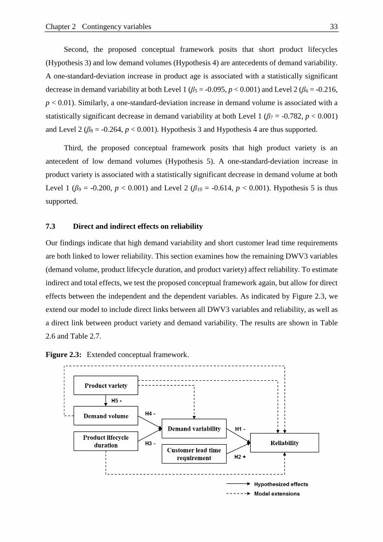
Chapter 2 Contingency variables 33
Second, the proposed conceptual framework posits that short product lifecycles
(Hypothesis 3) and low demand volumes (Hypothesis 4) are antecedents of demand variability.
A one-standard-deviation increase in product age is associated with a statistically significant
decrease in demand variability at both Level 1 (β5 = -0.095, p < 0.001) and Level 2 (β6 = -0.216,
p < 0.01). Similarly, a one-standard-deviation increase in demand volume is associated with a
statistically significant decrease in demand variability at both Level 1 (β7 = -0.782, p < 0.001)
and Level 2 (β8 = -0.264, p < 0.001). Hypothesis 3 and Hypothesis 4 are thus supported.
Third, the proposed conceptual framework posits that high product variety is an
antecedent of low demand volumes (Hypothesis 5). A one-standard-deviation increase in
product variety is associated with a statistically significant decrease in demand volume at both
Level 1 (β9 = -0.200, p < 0.001) and Level 2 (β10 = -0.614, p < 0.001). Hypothesis 5 is thus
supported.
7.3 Direct and indirect effects on reliability
Our findings indicate that high demand variability and short customer lead time requirements
are both linked to lower reliability. This section examines how the remaining DWV3 variables
(demand volume, product lifecycle duration, and product variety) affect reliability. To estimate
indirect and total effects, we test the proposed conceptual framework again, but allow for direct
effects between the independent and the dependent variables. As indicated by Figure 2.3, we
extend our model to include direct links between all DWV3 variables and reliability, as well as
a direct link between product variety and demand variability. The results are shown in Table
2.6 and Table 2.7.
Figure 2.3: Extended conceptual framework.
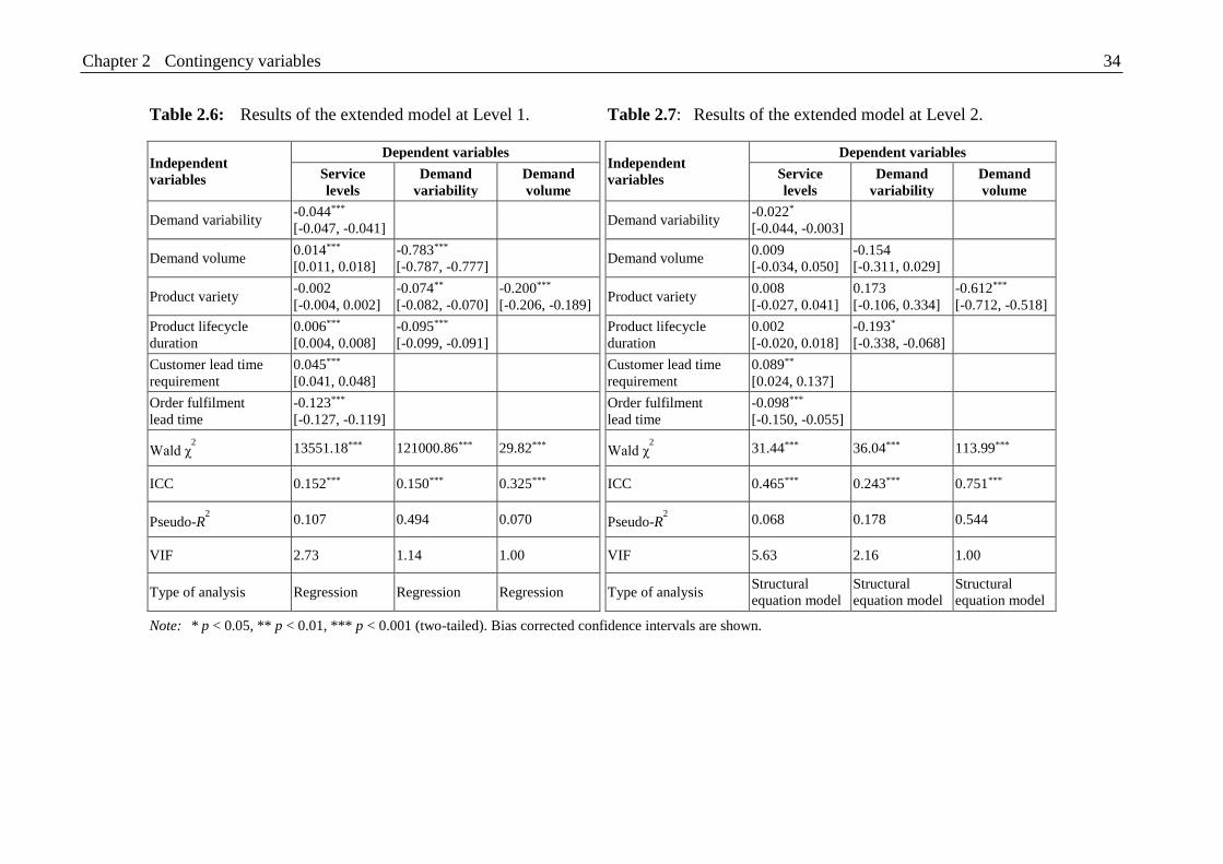
Chapter 2 Contingency variables 34
Table 2.6: Results of the extended model at Level 1. Table 2.7: Results of the extended model at Level 2.
Independent
variables
Dependent variables Independent
variables
Dependent variables
Service
levels
Demand
variability
Demand
volume
Service
levels
Demand
variability
Demand
volume
Demand variability -0.044***
[-0.047, -0.041]
Demand variability
-0.022*
[-0.044, -0.003]
Demand volume 0.014***
[0.011, 0.018]
-0.783***
[-0.787, -0.777]
Demand volume
0.009
[-0.034, 0.050]
-0.154
[-0.311, 0.029]
Product variety -0.002
[-0.004, 0.002]
-0.074**
[-0.082, -0.070]
-0.200***
[-0.206, -0.189]
Product variety
0.008
[-0.027, 0.041]
0.173
[-0.106, 0.334]
-0.612***
[-0.712, -0.518]
Product lifecycle
duration
0.006***
[0.004, 0.008]
-0.095***
[-0.099, -0.091]
Product lifecycle
duration
0.002
[-0.020, 0.018]
-0.193*
[-0.338, -0.068]
Customer lead time
requirement
0.045***
[0.041, 0.048]
Customer lead time
requirement
0.089**
[0.024, 0.137]
Order fulfilment
lead time
-0.123***
[-0.127, -0.119]
Order fulfilment
lead time
-0.098***
[-0.150, -0.055]
Wald χ2 13551.18*** 121000.86*** 29.82***
Wald χ
2 31.44*** 36.04*** 113.99***
ICC 0.152*** 0.150*** 0.325*** ICC 0.465*** 0.243*** 0.751***
Pseudo-R2 0.107 0.494 0.070
Pseudo-R
2 0.068 0.178 0.544
VIF 2.73 1.14 1.00 VIF 5.63 2.16 1.00
Type of analysis Regression Regression Regression Type of analysis
Structural
equation model
Structural
equation model
Structural
equation model
Note: * p < 0.05, ** p < 0.01, *** p < 0.001 (two-tailed). Bias corrected confidence intervals are shown.

Chapter 2 Contingency variables 35
Regarding demand volume, our findings confirm statistically significant direct, indirect
and total effects on reliability at Level 1. Demand volume has an indirect and positive link to
reliability that is mediated by demand variability (β11 = 0.035, p < 0.001). As the direct
relationship between demand volume and reliability also is positive and statistically significant
(β12 = 0.014, p < 0.001), the total effect of demand volume on reliability is positive and
statistically significant as well (β13 = 0.049, p < 0.001).
At Level 2, however, none of the examined relationships between demand volume and
reliability are statistically significant. When controlling for product variety, the link between
demand volume and demand variability is no longer statistically significant (β14 = -0.154, p =
0.082). One likely reason is that the strong correlations between product variety, demand
volume and product lifecycle duration at Level 2 (> 50%) lead to a loss of power. As a result,
the indirect link between demand volume and reliability is not statistically significant (β15 =
0.003, p = 0.253). Since the direct effect of demand volume on reliability is not statistically
significant either (β16 = 0.009, p = 0.673), there is no statistically significant total effect of
demand volume on reliability at Level 2 (β17 = 0.012, p = 0.553).
Regarding product lifecycle duration, our findings are very similar to the link between
demand volume and reliability. At Level 1, product lifecycle duration has statistically
significant direct, indirect and total effects on reliability. Product lifecycle duration has an
indirect and positive link to reliability that is mediated by demand variability (β18 = 0.004, p <
0.001). As the direct relationship between product lifecycle duration and reliability is also
positive and statistically significant (β19 = 0.006, p < 0.001), the total effect of product lifecycle
duration on reliability is positive and statistically significant as well (β20 = 0.010, p < 0.001).
However, at Level 2, neither the direct effect (β21 = 0.002, p = 0.882), the indirect effect (β22 =
0.004, p = 0.122) nor the total effect (β23 = 0.006, p = 0.558) of product lifecycle duration on
reliability are statistically significant.
Regarding product variety, our findings indicate that higher product variety is indirectly
linked to higher demand variability at both Level 1 and Level 2. At Level 1, both the indirect
effect via demand volume (β24 = 0.156, p < 0.001) and the total effect (β25 = 0.080, p < 0.01)
on demand variability are statistically significant. At Level 2, the effect of product variety on
demand variability is only partially mediated by demand volume. As a result, only the total
effect is positive and significant (β26 = 0.288, p < 0.01) whereas the indirect effect is positive
but not statistically significant (β27 = 0.095, p = 0.158). Our findings therefore indicate that
Chapter 2 Contingency variables 36
product variety – similar to demand volume and product lifecycle duration – is an antecedent
of demand variability.
However, we do not find support for a significant relationship between product variety
and reliability. At Level 1, there is a statistically significant indirect link between product
variety and reliability that is mediated by demand variability (β28 = -0.004, p < 0.01).
Nonetheless, the total effect of product variety on reliability fails to be significant (β29 = 0.000,
p = 0.978), since there is no significant direct link between the two variables (β30 = 0.002, p =
0.822). At Level 2, neither the direct effect (β31 = 0.008, p = 0.666), the indirect effect via
demand variability (β32 = -0.006, p = 0.132) nor the total effect (β33 = 0.001, p = 0.942) of
product variety on reliability are significant.
Discussion
8.1 Demand variability and customer lead time requirements
Our findings link high demand variability and short customer lead time requirements to
significantly lower reliability. At Level 1, high demand variability and short lead time
requirements are associated with approximately 4.4ppt lower reliability. At Level 2, the effect
of customer lead time requirements on reliability is even higher: a one standard deviation
decrease in lead time requirements is associated with a 9.2ppt decrease in reliability. The effect
of demand variability on reliability is lower at Level 2 than at Level 1 (2.2ppt), but it is still
significant at the 95% level. Our findings therefore consistently indicate that both high demand
and short customer lead time requirements make it harder to fulfil demand according to
customer specifications, ceteris paribus.
8.2 Demand volume and product lifecycle duration
On the contrary, our findings fail to consistently link low demand volumes and short product
lifecycles to lower reliability. At Level 2, there are no statistically significant direct effects of
demand volumes and product lifecycles on reliability. At Level 1, the effects are statistically
significant, but much lower than the effect of demand variability on reliability. Compared to
the effect demand variability, the direct effect of demand volume on reliability is more than
three times lower (1.4ppt instead of 4.4ppt). Similarly, the direct effect of product lifecycle
duration on reliability is more than seven times lower (0.6ppt instead of 4.4ppt). Low demand
volumes and short product lifecycle therefore only marginally decrease the ability of supply
chains to fulfil demand as requested, ceteris paribus.
Chapter 2 Contingency variables 37
However, our findings consistently link lower demand volumes and short product
lifecycles to higher demand variability. The tested effects are statistically significant and have
similar effect sizes with one exception: the link between demand volume and demand
variability is particularly strong at Level 1. A one-standard-deviation decrease in volume is
associated with a 0.8-standard-deviation increase in demand variability at that level of analysis.
Our findings therefore confirm that low demand volumes and short product lifecycles are
antecedent of demand variability.
8.3 Product variety
Our findings indicate a strong link between product variety and volume at both levels of
analysis. As a result, there is also an indirect link between product variety and demand
variability that is mediated by demand volume. Consequently, high product variety is associated
with significantly lower demand variability at both Level 1 and Level 2. Our findings therefore
indicate that product variety is an antecedent of demand variability as well.
Conclusion
9.1 Implications
This study intends to take a first step towards disambiguating which contingencies are important
for setting the competitive priorities of supply chains. For this purpose, we have examined the
effects hypothesized to be underlying the five most frequently cited contingency variables that
are referred to as DWV3.
Our findings consistently link high demand variability and short customer lead time
requirements to significantly lower reliability. Companies therefore need to consider these
variables when developing supply chain strategies to evaluate whether they require market
mediation capabilities to fulfil demand as requested by customers.
However, for the remaining DWV3 variables, we do not find a consistent direct link to
reliability. We therefore propose that managers seeking to determine whether they require
market mediation capabilities to reliably fulfil demand focus on examining the level of demand
variability and the length of lead time requirements in their organization. Analysing demand
volume, product variety and product lifecycle duration for this purpose as well will likely lead
to only few additional insights at the expense of a more complex strategy formation process.
Chapter 2 Contingency variables 38
Hence, we instead propose that companies use these variables for verifying and analysing the
causes of variable demand.
If companies cluster products or business units that are similar regarding the contingency
variables of interest, they require additional variables for establishing external validity (Bacher
et al., 2010; Brusco et al., 2017; Ketchen and Shook, 1996). In case a cluster of products is
characterized by, for instance, high values for demand variability, it is important to rule out that
these values are not caused by measurement error or statistical artefacts. Since our findings
indicate that volume, variety and lifecycle duration are antecedents of demand variability, they
are candidate variables for this purpose. In addition, companies may also use these variables to
analyse the causes of high demand variability and for designing corresponding mitigation
strategies, as different causes of variability may require different kinds of responses (Slack,
1987).
Yet besides the insights our study provides for the roles of the DWV3 variables in the
strategy formation process, the typology introduced in Section 2 highlights that two types of
variables not examined as part of this research might also be relevant for setting competitive
priorities.
First, in addition to demand variability and short customer lead time requirements,
supply-related challenges in the operating environment may also make it harder to fulfil demand
as requested by customers. They may therefore necessitate higher investments in the market
mediation than indicated by demand variability and customer lead time requirements for
demand to be fulfilled reliably.
Second, contingencies influencing value of market mediation are potentially important
for deciding whether or not to invest in market mediation in a challenging operating
environment. Supply chain strategy literature typically assumes that volatility and higher
margins go hand-in-hand (e.g., Childerhouse and Towill, 2000; Mason-Jones et al., 2000).
However, as we will demonstrate in Study 3, the correlations between contribution margins and
challenges in the operating environment at our case company are low. Before investing in
market mediation, companies may therefore evaluate variables of this type to ensure that the
financial reward of avoiding shortages outweighs the associated costs.
Chapter 2 Contingency variables 39
9.2 Limitations and future research
Our study has two key methodological limitations. First, we have analysed a single time period.
Even though we consider the DWV3 variables plausibly exogenous predictors, we cannot rule
out the threat of simultaneity completely (Ketokivi and McIntosh, 2017). Second, we have
analysed data from a single company. Even though our dataset provides considerable variance,
we cannot rule out that one might observe a change in effects when analysing data from a
different company or a different industry. As a result, there is a need for replication and
validation studies.
Further research is also needed to examine the effects underlying supply-related
challenges in the operating environment and variables influencing the value of market
mediation. Ho et al. (2005), for instance, propose that companies measure manufacturing-
related and supplier-related uncertainties using a set of seven reflective indicators. Future
studies may analyse whether a more parsimonious set of measures that is available in company
databases suffices for this purpose as well. Similarly, future studies may evaluate which
contingencies are important for approximating the value of market mediation and how these
contingencies could be measured.

Chapter 2 Contingency variables 40
Chapter 3 Supply chain segmentation 41
Chapter 3 Supply chain segmentation:
A data-driven approach
Co-author:
Moritz Fleischmann
Chair of Logistics and Supply Chain Management, Business School, University of
Mannheim, Germany
Abstract
For many companies, a single supply chain setup is not sufficient for fulfilling the divergent
needs of a heterogeneous product and customer portfolio. An emergent practice is thus to
“segment” supply chains: companies develop different supply chain strategies for different
parts of their business. While the extant literature largely forms supply chain segments
qualitatively, our study introduces two quantitative methods: clustering and classification. We
employ these methods at a leading chemicals manufacturer and compare our results to segments
the company had formed using managers’ tacit knowledge. Our findings indicate that managers
may choose segments that do not reflect the needs of their business environment, consequently
pursuing supply chain strategies that adversely affect financial performance. Clustering and
classification help managers detect such segment-environment mismatches and thus serve as
valuable tools for challenging managers’ judgment when conducting a supply chain
segmentation.

Chapter 3 Supply chain segmentation 42
Motivation
Companies frequently offer a wide variety of products to a range of different customers.
Oftentimes, these products and customers are heterogeneous regarding the type of supply chain
they require. Consider, for instance, the well-known difference between innovative and
functional products: while the former require a supply chain that excels at matching supply and
demand in a challenging operating environment, the latter require a supply chain that
emphasizes efficiency (Fisher, 1997). Yet it is not uncommon for companies to sell both
innovative and functional products (Childerhouse et al., 2002). As a result, supply chain
segmentation (SCS) has become an emergent practice. It describes the process of dividing a
heterogeneous set of products or customers into groups (“segments”) that impose similar
requirements on the supply chain. For each of these segments, a tailored supply chain strategy
is developed.
SCS, therefore, allows companies to more accurately tailor their supply chain capabilities
and structures to the requirements of their business. Compared to a company with a single
supply chain strategy, a company with a tailored strategy for each segment may operate some
parts of its business at lower cost (e.g., functional products or cost-conscious customers) and
extract higher revenues from other parts of its business (e.g., additional service for service-
oriented customers or innovative products). As a result, SCS is considered one of the most
effective levers for improving supply chain performance (Rexhausen et al., 2012) and has been
linked to lower inventories, higher service levels and lower logistics cost (Mayer et al., 2009).
A recent survey by Gartner, a consultancy, concludes that “an overwhelming 95% of [chief
supply chain officers] expect to invest in supply chain segmentation in 2016, with 35% calling
it a top priority” (Gartner, 2016a).
Despite practitioners’ interest in the topic, the number of corresponding studies is limited
so far. A key characteristic of the extant literature on SCS is a qualitative approach to segment
formation: segments are formed using managers’ tacit knowledge, without a systematic data
analysis.
This approach has drawbacks. Managers’ tacit knowledge is subjective; relevant clusters
of products or customers may remain undetected as a result (Foedermayr and Diamantopoulos,
2008). Especially if product or customer portfolios are broad and heterogeneous, it is unlikely
that managers will have a comprehensive overview of all relevant segmentation criteria and
objects (Wedel, 2000). A SCS initiative that exclusively relies on managers’ tacit knowledge
can thus only provide limited insights.

Chapter 3 Supply chain segmentation 43
Consequently, authors of segmentation methodologies in marketing urge practitioners to
refrain from solely relying on the qualitative approach (Foedermayr and Diamantopoulos, 2008;
Wedel, 2000). There are many examples of segmentation initiatives in other areas of business
research that employ data analysis to derive segments (Ngai et al., 2009). The supply chain
community, however, appears to be lagging behind in this regard: with one exception
(Langenberg et al., 2012), all reviewed articles in scholarly journals on SCS exclusively rely
on managers’ tacit knowledge for this purpose. Strikingly, the two most commonly employed
methods for deriving segments in other areas of business research – clustering and classification
(Ngai et al., 2009) – have not been used in studies on SCS so far.
Our study thus employs clustering and classification to form supply chain segments.
Specifically, we use data from the chemicals manufacturer BASF to form segments
quantitatively and compare our results to segments the company had previously formed without
data analysis. Based on our findings, we are able to deduce several managerial insights on this
issue. In particular, we address the following questions. How can companies use clustering and
classification for a SCS? What insights do these methods generate relative to qualitative
approaches?
The remainder of this article proceeds as follows. In Section 2, we review extant
qualitative and quantitative approaches in SCS literature and outline how clustering and
classification can remedy their shortcomings. Section 3 introduces the case company and
outlines its qualitative approach to forming segments. In Section 4, we form segments using
clustering, and we compare the results to the company’s qualitative segments in Section 5. In
Section 6, we highlight the need to update segments periodically and demonstrate how
classification can be employed for this purpose. Section 7 discusses the implications of our
findings and the limitations of our work.
Related literature
This section reviews the extant approaches to forming supply chain segments and outlines how
clustering and classification may help remedy their shortcomings.
2.1 Qualitative approaches
The vast majority of studies on SCS forms segments without data analysis. The first study on
the topic introduces a qualitative approach claiming that “clustering is more an art than a
science” (Fuller et al., 1993). It advises managers to examine for each product successively

Chapter 3 Supply chain segmentation 44
whether a distinct supply chain setup is needed, and to form a new segment only if the expected
benefits outweigh the additional complexity costs.
Aitken et al. (2005), Childerhouse et al. (2002) and Godsell et al. (2011) advocate a
different case-by-case approach. First, managers collectively decide on a set of segments.
Second, they assess for each product individually which segment fits best. Variables such as
demand variability and contribution margins (Godsell et al., 2011) or the stage of the product
lifecycle (Aitken et al., 2005; Childerhouse et al., 2002) are taken into account for this purpose.
Christopher et al. (2006) and Christopher and Towill (2002) neither outline how they
form segments nor how they allocate products or customers to segments. Instead, they introduce
a set of generic supply chain strategies and describe how companies have adopted these
strategies for different parts of their business (e.g., 80% of the business is “lean” and 20% is
“agile”). However, in a later study, the authors disclose that the introduced strategies were
determined by “hunch” rather than data analysis, and call for the use of “advanced analytics”
for SCS (Christopher et al., 2009).
Roscoe and Baker (2014) present a special case, where a company has formed supply
chain segments that correspond to its market segments. As each market segment is served with
a distinct product offering at the case company, products are allocated to supply chain segments
depending on the market segment that they serve.
Finally, a stream of publications proposes a narrower approach to SCS (Langenberg et
al., 2012; Lovell et al., 2005; Payne and Peters, 2004). Rather than differentiating supply chain
strategies between segments, these publications only differentiate individual design choices
such as the speed of the transportation mode or sourcing locations. With one exception
(Langenberg et al., 2012), the number and type of segments is determined based on managers’
judgment. Products are then allocated to segments based on threshold values. Lovell et al.
(2005) determine whether a product should be shipped by sea or air based on its value and
chargeable weight. Similarly, Payne and Peters (2004) establish thresholds (e.g., the minimum
number of order lines per year) that determine whether products should be held centrally or
locally.
The main advantage of the outlined qualitative approaches is that they require neither the
availability of data nor the knowledge of statistics software. However, segments formed based
on managers’ judgment alone can only provide limited new insights, as no new information
enters the segment formation process (Foedermayr and Diamantopoulos, 2008). Especially if a

Chapter 3 Supply chain segmentation 45
large number of criteria needs to be analysed when forming segments, managers tend to have
trouble identifying products or customers that are similar with respect to the criteria of interest
(Wedel, 2000). Consequently, segmentation procedures without data analysis are considered
“probably the simplest but least effective” (Wedel, 2000).
2.2 Quantitative approach
Langenberg et al. (2012) are the first to recognize the resulting need for “profound quantitative
analysis”. They introduce a model that matches the product portfolio of a company with a set
of supply chains. It assumes that companies hold a diverse portfolio of functional and
innovative products for which product characteristics related to cost (holding, stockout,
procurement and order setup), demand (mean and standard deviation) and production lead times
are known. Further, the model assumes that companies have a portfolio of supply chain options
at their disposal with known supply-chain-specific lead times and procurement cost. To form
segments, Langenberg et al. (2012) employ a branch-and-bound algorithm that selects a subset
of the supply chain portfolio and allocates products to these supply chains with the goal of
minimizing total cost.
An advantage of this approach is that it finds the “optimal” set of segments, i.e., segments
that minimize the sum of all considered costs. However, it presumes that managers have a
portfolio of supply chain design options with quantifiable performance implications at their
disposal. This assumption holds only if the SCS focuses on isolated design decisions: in their
study, Langenberg et al. (2012) assess a set of 20 different sourcing and shipment options with
quantified implications for lead times, procurement and transportation costs. Yet, if the goal of
the SCS is to assess different strategic directions, a broader set of performance measures is
affected and performance implications are harder to quantify (APICS, 2016).
Langenberg et al. (2012) acknowledge this limitation and highlight that their model
provides guidance “at the tactical [rather than the strategic] level of decision-making”.
Consequently, as most studies on SCS seek to form segments that serve as a basis for tailored
supply chain strategies, there is a need to introduce a different set of quantitative methods to
SCS.
2.3 Clustering
Clustering is the unsupervised learning task of subdividing a set of heterogeneous objects into
groups that are internally homogenous and heterogeneous amongst each other (Bacher et al.,
Chapter 3 Supply chain segmentation 46
2010; Clarke et al., 2009) . When conducting a cluster analysis, critical decisions include
selecting segmentation criteria, selecting a clustering procedure and assessing cluster
solutions.
Selecting segmentation criteria for a cluster analysis entails a trade-off. On the one hand,
if important criteria are omitted, the obtained solutions fail to adequately reflect the context of
interest. On the other hand, irrelevant or redundant criteria may distort the cluster analysis and
thus prevent meaningful solutions from being found (Ketchen and Shook, 1996; Milligan,
1996). The screening and pre-testing of candidate criteria is therefore a critical part of a cluster
analysis (Brusco et al., 2017).
Clustering procedures are either heuristics or model-based (Bacher et al., 2010). Heuristic
clustering procedures such as K-Means or Ward’s method are the most popular in the operations
management area. However, in recent years, model-based procedures are being increasingly
employed as well (Brusco et al., 2012). Whereas heuristic procedures aim to find a local
optimum within a reasonable amount of time, model-based procedures assume a probability
model underlying the data. As a result, most heuristic procedures require a distinct classification
of objects to clusters, whereas model-based procedures allow objects to belong to multiple
clusters (Bacher et al., 2010). The choice of the clustering method therefore depends on how
clearly clusters are separated in the data and on whether overlapping clusters are permissible
(Everitt et al., 2011).
Finally, the assessment of cluster solutions evaluates whether the obtained solutions
suffice for reaching the goal of the analysis (Bacher et al., 2010). The assessment comprises the
examination of technical features such as within-cluster heterogeneity and between-cluster
homogeneity. It also evaluates the interpretability of clusters and tests their stability.
Performing a cluster analysis therefore not only requires knowledge of the technical
features of the analysis, but also of the context in which the analysis takes place. Despite these
requirements, cluster analysis is the most popular method for data-driven segmentation
initiatives in business research (Ngai et al., 2009) and popular for market segmentation in
particular (Wedel, 2000). When conducting a market segmentation, companies may use cluster
analysis to group customers that are similar regarding their response to marketing activities
(Foedermayr and Diamantopoulos, 2008). When conducting a SCS, companies may use cluster
analysis to group products or customers that are similar regarding the type of supply chain they
require. In doing so, cluster analysis may discover groups of similar products or customers that
Chapter 3 Supply chain segmentation 47
managers would not have discovered using tacit knowledge alone. Unlike the quantitative
approach by Langenberg et al. (2012), managers do not need to specify supply chain designs or
strategies upfront.
2.4 Classification
Contrary to clustering, classification is a supervised learning task (Duda et al., 2012). Whereas
clustering aims to uncover hidden patterns in the data, classification assigns objects to a
predetermined set of classes (Breiman, 2001). First, the classification algorithm is trained using
a “training dataset” with a pre-established allocation of objects to classes. The trained algorithm
then allocates objects to classes for a “test dataset” where the allocation of objects to classes is
unknown.
Available classification procedures range from probabilistic methods, decision trees, rule-
based methods, instance-based methods, support vector machines to neural networks
(Aggarwal, 2015). They differ regarding a number of characteristics such as predictive
accuracy, training speed, the ability to handle missing data or the amount of parameter tuning
required. K-Nearest Neighbours (KNN) algorithms, for instance, are instance-based methods
that are simple to implement and make few assumptions about the underlying data structure,
but they are resource-intensive. Neural networks are fast to run once they are trained, but require
considerable tuning of input parameters and it is hard to understand how these algorithms arrive
at classifications (Kotsiantis, 2007). Similar to clustering, the choice of the classification
method therefore depends on the dataset and the application scenario.
In the operations management area, classification currently receives significant attention
due to the trend topic “Internet of Things”. Application areas include the prediction of machine
failures (Peng et al., 2010) and the large-scale analysis of sensor data (Perera et al., 2014). In
the context of a SCS, classification algorithms are of interest once companies have established
a preliminary set of segments via clustering or a qualitative approach.
Companies may use classification to review the allocation of objects to segments that they
have established qualitatively. When managers allocate objects to segments as part of a
qualitative approach, they implicitly consider a set of segmentation criteria (e.g., “does the
product that needs to be allocated have a low or a high contribution margin?”). If data is
available for these criteria, managers may compose a training dataset of archetype objects (e.g.,
products or customers) for each segment and then classify the remaining objects using a
classification algorithm.

Chapter 3 Supply chain segmentation 48
Similarly, companies may use classification algorithms to update segments obtained from
clustering. Companies’ product and customer portfolios are constantly changing – accordingly
the allocation of objects to segments needs to be reviewed periodically. As products mature, for
instance, demand variability and contribution margins are likely to decrease (Aitken et al.,
2005). Once the segmentation criteria of the objects in a company’s portfolio change, the
company may employ a classification algorithm to review the allocation of objects to segments
using the results of the initial cluster analysis as the training dataset. Finally, classification
algorithms are also useful to allocate new products or customers to existing supply chain
segments.
Companies may thus use classification procedures to update or challenge existing
segments. The extant literature acknowledges the importance of regularly reviewing supply
chain segments (Godsell et al., 2011; Seifert and Langenberg, 2011). Nonetheless, we are not
aware of any studies on SCS that employ classification.
Case company
3.1 Company profile
Arguably, one of the best-suited companies to examine how companies can use clustering and
classification for a SCS is the chemicals manufacturer BASF. Contrary to its competitors,
BASF embraces the “Verbund”-concept: the company controls value streams that span from
basic chemicals to high-value-added products such as coatings and crop protection agents
(BASF SE, 2016b). While this diversity achieves annual cost savings in excess of 1€ billion in
logistics and production, it aggravates supply chain complexity: a business unit producing basic
chemicals requires a different supply chain than a business unit producing high-value crop
protection. The former operates in a stable low-margin environment and thus prioritizes cost-
efficiency. The latter operates in a volatile high-margin environment and thus requires
capabilities for matching demand and supply (Fisher, 1997). Due to the scope of its operations,
BASF is considerably diverse regarding the type of supply chain different parts of its business
require.
To remedy this diversity, BASF initiated a SCS in the years 2013 and 2014. Goals
included finding a common terminology to communicate supply chain needs, obtaining a better
overview of how supply chain needs are distributed across the business unit portfolio, and
helping business units tailor their supply chains to the needs of their business environment. As
Chapter 3 Supply chain segmentation 49
quantitative approaches to deriving supply chain segments were missing at that time, the
company decided to form segments based on managers’ judgment.
3.2 Qualitative segments
BASF’s SCS project initially consisted of two phases. First, to come up with a set of supply
chain segments, the company put together a focus group consisting of their supply chain
strategy team, external consultants and supply chain leaders of business units. Second, after the
focus group had decided on a set of four segments, business unit supply chain leaders were
asked to assign their business unit to one of the supply chain segments. If they considered their
product or customer portfolio too diverse for a single segment, they had the option of
subdividing their business unit and choosing different segments for different parts.
Three of the segments identified by the qualitative approach have been widely discussed
in textbooks and supply chain strategy literature: Lean, Leagile and Agile (e.g., Agarwal et al.,
2006; Mason-Jones et al., 2000; Naylor et al., 1999).
The “Lean” segment comprises cost-sensitive business units with a stable operating
environment. Consequently, the goal of these business units is to ensure reliable supply at
competitive costs through practices such as level scheduling and just-in-time production.
The “Leagile” and the “Agile” segments comprise business units that operate in a volatile
environment with customers willing to pay a premium. In the Agile segment, customers tolerate
relatively long lead times. Business units in the Agile segment can therefore use flexible make-
to-order production to deal with uncertainties. In the Leagile segment, customers only tolerate
short lead times. Business units in the Leagile segment therefore rely on a postponement
strategy that emphasizes cost-efficiency upstream and flexibility downstream of the decoupling
point.
The fourth segment is company-specific. We refrain from discussing it in this paper to
protect the proprietary information of BASF. However, it is also only relevant for a small
minority of business units (fewer than 2% of the company’s business units). When comparing
the qualitative to the quantitative approach, we will focus on the former three supply chain
segments.
Chapter 3 Supply chain segmentation 50
Clustering
4.1 Dataset
4.1.1 Unit of analysis
Studies on SCS differ regarding the unit of analysis they choose for subdividing businesses into
groups that require distinct supply chain strategies. Some studies segment products (Aitken et
al., 2005; Childerhouse et al., 2002; Christopher et al., 2006; Christopher and Towill, 2002;
Christopher et al., 2009; Langenberg et al., 2012; Lovell et al., 2005; Payne and Peters, 2004),
whereas others segment customers (Christopher and Gattorna, 2005; Godsell et al., 2006).
We choose a more aggregated unit of analysis by clustering business units. We cluster
business units rather than products or customers for three reasons. First, clustering business
units ensures comparability to the company’s qualitative approach. Second, data on
contribution margins – a critical segmentation criterion – is only available at the business-unit-
level. Third, the business units in our dataset are organized according to the products they sell
(e.g., herbicides versus fungicides) and according to the markets they serve (e.g., Europe or
Asia) (BASF SE, 2017). Clustering business units therefore takes into consideration that supply
chain strategies account for both product and customer/market characteristics.
4.1.2 Sampling
Our dataset covers the entire company except for its oil and gas division for the years 2013 and
2014. As a result, it captures approximately 80% of the company’s revenues during the
examined period (BASF SE, 2015). In total, the dataset comprises 228 business units.
We exclude business units with annual sales below 1 million € or fewer than 1,000 orders
annually to ensure that only business units with sufficient supply-chain-related activities are
included. Further, we exclude one business unit with missing data and one business unit that
was not reliably integrated in the company’s databases at the time. The final sample therefore
comprises 181 observations and is identical to sample of business units employed in Chapter 2.
4.2 Segmentation criteria
Segmentation criteria are contingency variables considered important for deciding which
supply chain strategy to pursue. Arguably the most prominent framework of such variables is
the distinction between functional and innovative products (Fisher, 1997). The previous chapter
has subdivided the characteristics of functional and innovative products into two categories:
Chapter 3 Supply chain segmentation 51
challenges in the operating environment and variables influencing the value of matching supply
and demand. We use this categorization as guidance for selecting segmentation criteria.
4.2.1 Challenges in the operating environment
Challenges in the operating environment inhibit the ability to match supply and demand, ceteris
paribus. An operating environment characterized by unexpected changes in demand, for
example, requires a supply chain that emphasizes flexibility and agility (Gligor, 2015;
Merschmann and Thonemann, 2011). Similarly, if customers demand short lead times, supply
chains need to be sufficiently responsive to achieve on-time delivery nonetheless (de Treville
et al., 2014a).
An examination of frameworks for supply chain or manufacturing strategies reveals that
demand uncertainty and time pressure are indeed two of the most important challenges imposed
by operating environments. According to Fisher (1997), challenges in the operating
environment comprise different causes of demand uncertainty (short lifecycles, forecast error
and high product variety) as well as the time granted by customers to fulfil orders. The same is
true for the DWV3 framework by Christopher et al. (2009) which also considers different
sources of demand uncertainty (demand variability and volume, product variety and the product
lifecycle) as well as the customer lead time requirement. Olhager (2003) explicitly maps
challenges of the operating environment along a time-related and a demand-related dimension.
In line with these frameworks, we include variables that approximate demand uncertainty and
time pressure as segmentation criteria in the cluster analysis.
Contingency variables proposed in the extant literature for approximating time pressure
include the time window for delivery (Christopher et al., 2009), market standards for lead times
(Fisher, 1997) and the ratio between customers’ lead time requirements and the production lead
time (Olhager, 2003). As our dataset does not feature information on production lead times, we
use customers’ lead time requirements to approximate time-related challenges. We measure
lead time requirements by the number of days customers grant between order placement and
the requested delivery date.
The most frequently proposed variable in the extant literature on supply chain strategy
for approximating demand uncertainty using company data is demand variability (Basnet and
Seuring, 2016). Demand variability captures both expected and unexpected changes in demand.
Following Aitken et al. (2005) and Christopher et al. (2009), we measure demand variability as
the coefficient of variation of weekly sales.
Chapter 3 Supply chain segmentation 52
4.2.2 Value of matching supply and demand
Even if demand uncertainty and time pressure increase the need to invest in capabilities that
improve the match between supply and demand, this does not imply that such investments
should necessarily be taken. Managers need to ensure that the benefits of preventing supply and
demand mismatches clearly outweigh the associated costs.
Variables approximating the value of matching supply and demand include contribution
margins, contract penalties, goodwill loss and the salvage value of products (Langenberg et al.,
2012). Due to data availability, this study focuses on contribution margins. Segmentation
criteria used in the main body of this study are thus demand variability, customer lead time
requirements and contribution margins. Table 3.1 provides a summary of all measures.
Table 3.1: Variable descriptions and measurement.
Variable Measurement
Seg
men
tati
on
cri
teria
Demand variability Coefficient of variation of weekly sales
(logarithm, standardized)
Customer lead time
requirements
Average number of days customers grant between the initial
order entry and the requested delivery date
(logarithm, standardized)
Contribution margins Average selling price minus the average variable cost per unit
(standardized)
Demand uncertainty
(Appendix B) Factor analysis output
Time pressure
(Appendix B) Factor analysis output
Ex
tern
al
va
lid
ity
Product lifecycle duration Average product age
(logarithm, standardized)
Demand volume Average sales per product
(logarithm, standardized)
Product variety Number of products in the business unit’s portfolio
(logarithm, standardized)
Mis
ma
tch
-per
form
an
ce l
ink
Self-assigned segments Proportion of the business unit’s sales assigned to the Lean,
Leagile or Agile segment by managers
Segments proposed by the
cluster analysis
Lean, Leagile, Agile or Basic Service
(categorical)
Mismatches
Proportion of the business unit’s sales for which the self-
assigned segment does not correspond to the segment
proposed by the cluster analysis
Business unit size Business unit revenues during the examined period
(logarithm, standardized)
Financial performance Return on sales
Variables with diminishing marginal effects are logarithmized. Variables used as segmentation criteria
or for assessing external validity are standardized to render their scales comparable.
Chapter 3 Supply chain segmentation 53
4.3 Clustering procedure
Visual inspection of the data does not reveal a clear cluster structure. To deal with this issue –
which is common in segmentation initiatives – model-based procedures that allow overlapping
clusters have been developed (Brusco et al., 2012). We therefore perform the cluster analysis
using the model-based clustering algorithm Mclust. We select the Mclust algorithm because it
is available free of charge and offers a wide range of diagnostic tools (Fraley and Raftery, 2002).
4.4 Assessing cluster solutions
We follow a four-step approach to determine the number of clusters and evaluate cluster
solutions (Bacher et al., 2010).
4.4.1 Preselecting candidate solutions
We preselect a candidate set of cluster solutions by assessing measures of within-cluster
homogeneity, between-cluster heterogeneity and explained variance. The Bayesian Information
Criterion (BIC) weighs the incremental increase in the proportion of variance explained by an
additional cluster against the risk of overfitting the cluster solution to the data. As shown in
Table 3.2, the BIC proposes solutions with two, three or four clusters. In addition to the BIC,
we employ two standard metrics for assessing within-cluster homogeneity and between-cluster
heterogeneity (Brock et al., 2011). The Silhouette metric proposes a solution with two or four
clusters; the Dunn Index proposes a solution with two, three or four clusters.
Table 3.2: Statistical properties of the cluster solutions.
Statistical
properties
Number of clusters
1 2 3 4 5 6
BIC -1558.753 -1548.338 -1548.675 -1552.244 -1556.325 -1571.711
Silhouette 0.318 0.250 0.312 0.269 0.259
Dunn Index 0.053 0.055 0.055 0.040 0.032
Note: Bolded values indicate preferred solutions
4.4.2 Nominating the final solution
The goal of segmentation initiatives is to arrive at an actionable set of segments (Foedermayr
and Diamantopoulos, 2008): segments must be sufficiently homogeneous regarding the
examined criteria for determining the type of action required. In a quantitative SCS, clusters
therefore need to be sufficiently homogeneous for determining which supply chain strategy is
needed.
For this purpose, we evaluate the two-dimensional scatter plots in Figures 3.1-3.3. Each
figure shows one of the candidate solutions. The axis of the scatters depict the examined criteria.
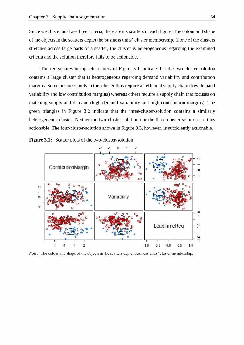
Chapter 3 Supply chain segmentation 54
Since we cluster analyse three criteria, there are six scatters in each figure. The colour and shape
of the objects in the scatters depict the business units’ cluster membership. If one of the clusters
stretches across large parts of a scatter, the cluster is heterogeneous regarding the examined
criteria and the solution therefore fails to be actionable.
The red squares in top-left scatters of Figure 3.1 indicate that the two-cluster-solution
contains a large cluster that is heterogeneous regarding demand variability and contribution
margins. Some business units in this cluster thus require an efficient supply chain (low demand
variability and low contribution margins) whereas others require a supply chain that focuses on
matching supply and demand (high demand variability and high contribution margins). The
green triangles in Figure 3.2 indicate that the three-cluster-solution contains a similarly
heterogeneous cluster. Neither the two-cluster-solution nor the three-cluster-solution are thus
actionable. The four-cluster-solution shown in Figure 3.3, however, is sufficiently actionable.
Figure 3.1: Scatter plots of the two-cluster-solution.
Note: The colour and shape of the objects in the scatters depict business units’ cluster membership.
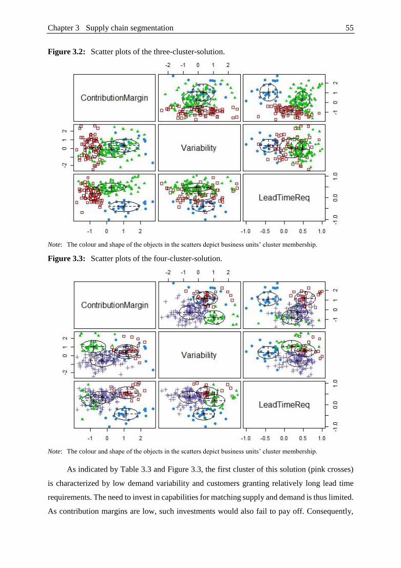
Chapter 3 Supply chain segmentation 55
Figure 3.2: Scatter plots of the three-cluster-solution.
Note: The colour and shape of the objects in the scatters depict business units’ cluster membership.
Figure 3.3: Scatter plots of the four-cluster-solution.
Note: The colour and shape of the objects in the scatters depict business units’ cluster membership.
As indicated by Table 3.3 and Figure 3.3, the first cluster of this solution (pink crosses)
is characterized by low demand variability and customers granting relatively long lead time
requirements. The need to invest in capabilities for matching supply and demand is thus limited.
As contribution margins are low, such investments would also fail to pay off. Consequently,

Chapter 3 Supply chain segmentation 56
the competitive priority of business units in this cluster should be cost efficiency while ensuring
that service levels are sufficiently high. As the first cluster is thus similar to the Lean segment
derived by the judgmental approach, we will refer to this cluster as “Lean”.
The second cluster (red squares) and the third cluster (blue dots) both have above average
demand variability and contribution margins. Consequently, they require capabilities for
matching supply and demand such as responsiveness or agility (de Treville et al., 2014a; Gligor
et al., 2015). Customer lead time requirements are relatively short in the second cluster and
relatively long in the third cluster. Business units in the second cluster thus require capabilities
for matching supply and demand at short notice, whereas business units in the third cluster may
for instance employ flexible make-to-order production to deal with the variable demand. Since
the two clusters are therefore similar to the Leagile and the Agile segments derived by the
qualitative approach, we will refer to the second cluster as “Leagile” and to the third as “Agile”.
High demand variability also characterizes business units in the fourth cluster (green
triangles). However, since contribution margins are low, the scope for investments in
capabilities for matching supply and demand is limited. The extant literature proposes two
strategies for such a context. First, business units may follow a portfolio alignment strategy by
eliminating low-margin and high-variability products from the portfolio (Barksdale and Harris,
1982; Godsell et al., 2011). Second, business units may distinguish between predictable “base”
demand and volatile “surge” demand: base demand is met with a cost-efficient supply chain
and surge demand is neglected at the expense of lower service levels (Christopher et al., 2006;
Christopher and Towill, 2002). In line with the latter strategy, we will refer to the fourth cluster
as “Basic Service”.
Table 3.3: Criteria and covariates of the four-cluster-solution (standardized).
Lean Leagile Agile Basic
Service
Cri
teri
a Contribution margins -0.31 1.10 1.16 -0.81
Demand variability -0.58 0.37 0.58 1.05
Customer lead time requirements 0.25 -1.75 0.76 -0.10
Co
var
iate
s Product lifecycle duration 0.35 -1.04 -0.46 0.04
Demand volume 0.35 -1.04 -0.23 -0.18
Product variety -0.36 1.19 0.53 -0.16
Number of business units 102 24 25 30
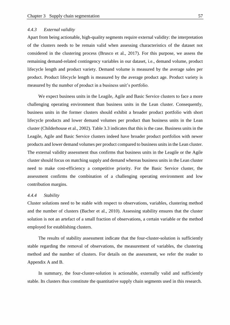
Chapter 3 Supply chain segmentation 57
4.4.3 External validity
Apart from being actionable, high-quality segments require external validity: the interpretation
of the clusters needs to be remain valid when assessing characteristics of the dataset not
considered in the clustering process (Brusco et al., 2017). For this purpose, we assess the
remaining demand-related contingency variables in our dataset, i.e., demand volume, product
lifecycle length and product variety. Demand volume is measured by the average sales per
product. Product lifecycle length is measured by the average product age. Product variety is
measured by the number of product in a business unit’s portfolio.
We expect business units in the Leagile, Agile and Basic Service clusters to face a more
challenging operating environment than business units in the Lean cluster. Consequently,
business units in the former clusters should exhibit a broader product portfolio with short
lifecycle products and lower demand volumes per product than business units in the Lean
cluster (Childerhouse et al., 2002). Table 3.3 indicates that this is the case. Business units in the
Leagile, Agile and Basic Service clusters indeed have broader product portfolios with newer
products and lower demand volumes per product compared to business units in the Lean cluster.
The external validity assessment thus confirms that business units in the Leagile or the Agile
cluster should focus on matching supply and demand whereas business units in the Lean cluster
need to make cost-efficiency a competitive priority. For the Basic Service cluster, the
assessment confirms the combination of a challenging operating environment and low
contribution margins.
4.4.4 Stability
Cluster solutions need to be stable with respect to observations, variables, clustering method
and the number of clusters (Bacher et al., 2010). Assessing stability ensures that the cluster
solution is not an artefact of a small fraction of observations, a certain variable or the method
employed for establishing clusters.
The results of stability assessment indicate that the four-cluster-solution is sufficiently
stable regarding the removal of observations, the measurement of variables, the clustering
method and the number of clusters. For details on the assessment, we refer the reader to
Appendix A and B.
In summary, the four-cluster-solution is actionable, externally valid and sufficiently
stable. Its clusters thus constitute the quantitative supply chain segments used in this research.
Chapter 3 Supply chain segmentation 58
Comparing quantitative and qualitative segments
The cluster analysis largely confirms the results of BASF’s qualitative approach: three clusters
correspond to the segments derived qualitatively (Lean, Leagile and Agile). However, it also
provides two novel insights. First, the qualitative approach does not identify the Basic Service
cluster. Second, the self-assignment of business units to segments often does not correspond to
the segment proposed by the cluster analysis. Such a mismatch occurs, for instance, if a business
unit assigns itself to the Leagile segment even though the cluster analysis suggests that the Lean
segment would be a better fit.
5.1 Mismatch-performance link
There are two potential causes for mismatches between self-assigned segments and segments
proposed by the cluster analysis.
On the one hand, falsely omitted segmentation criteria may have distorted the results of
the cluster analysis. For example, the segment propositions by the cluster analysis might be
inaccurate for business units in our sample supplying the automotive industry, since delivering
as requested is important in that industry regardless of contribution margins (Guiffrida and
Nagi, 2006). Thus, if falsely omitted criteria have caused mismatches between the self-assigned
and the proposed segments, these mismatches simply indicate that the segments derived
quantitatively are inadequate.
On the other hand, however, if mismatches result from business units selecting segments
that do not reflect the requirements of their business environment, adverse effects are likely. In
such cases, business units are pursuing supply chain strategies that overcharge or underserve
customers, which in turn leads to either unnecessarily high costs or lost sales (Fuller et al.,
1993). A mismatch between the self-assigned and the proposed segment caused by managers’
misjudgement should thus manifest itself in lower financial performance (Gligor, 2015; Wagner
et al., 2012).
Given the diligent criteria selection and given the stability of the derived segments, we
hypothesize that a significant proportion of mismatches indicates managers’ misjudgement as
illustrated by Figure 3.4.
Hypothesis 1: There is a negative relationship between mismatches and financial
performance.
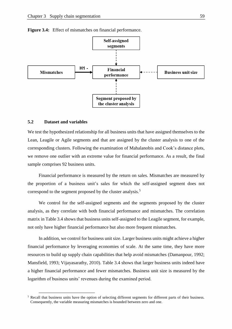
Chapter 3 Supply chain segmentation 59
Figure 3.4: Effect of mismatches on financial performance.
5.2 Dataset and variables
We test the hypothesized relationship for all business units that have assigned themselves to the
Lean, Leagile or Agile segments and that are assigned by the cluster analysis to one of the
corresponding clusters. Following the examination of Mahalanobis and Cook’s distance plots,
we remove one outlier with an extreme value for financial performance. As a result, the final
sample comprises 92 business units.
Financial performance is measured by the return on sales. Mismatches are measured by
the proportion of a business unit’s sales for which the self-assigned segment does not
correspond to the segment proposed by the cluster analysis.5
We control for the self-assigned segments and the segments proposed by the cluster
analysis, as they correlate with both financial performance and mismatches. The correlation
matrix in Table 3.4 shows that business units self-assigned to the Leagile segment, for example,
not only have higher financial performance but also more frequent mismatches.
In addition, we control for business unit size. Larger business units might achieve a higher
financial performance by leveraging economies of scale. At the same time, they have more
resources to build up supply chain capabilities that help avoid mismatches (Damanpour, 1992;
Mansfield, 1993; Vijayasarathy, 2010). Table 3.4 shows that larger business units indeed have
a higher financial performance and fewer mismatches. Business unit size is measured by the
logarithm of business units’ revenues during the examined period.
5 Recall that business units have the option of selecting different segments for different parts of their business.
Consequently, the variable measuring mismatches is bounded between zero and one.
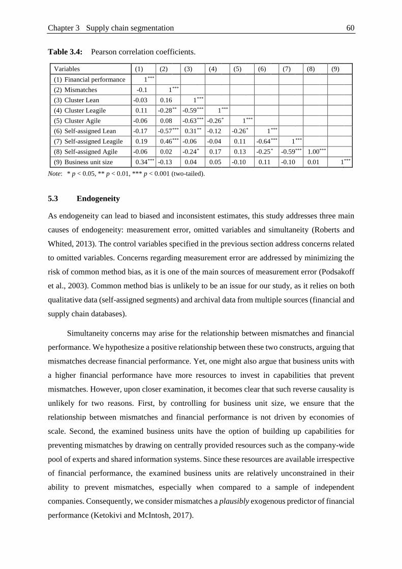
Chapter 3 Supply chain segmentation 60
Table 3.4: Pearson correlation coefficients.
Variables (1) (2) (3) (4) (5) (6) (7) (8) (9)
(1) Financial performance 1 ***
(2) Mismatches -0.1 1 ***
(3) Cluster Lean -0.03 0.16 1 ***
(4) Cluster Leagile 0.11 -0.28 ** -0.59 *** 1 ***
(5) Cluster Agile -0.06 0.08 -0.63 *** -0.26 * 1 ***
(6) Self-assigned Lean -0.17 -0.57 *** 0.31 ** -0.12 -0.26 * 1 ***
(7) Self-assigned Leagile 0.19 0.46 *** -0.06 -0.04 0.11 -0.64 *** 1 ***
(8) Self-assigned Agile -0.06 0.02 -0.24 * 0.17 0.13 -0.25 * -0.59 *** 1.00 ***
(9) Business unit size 0.34 *** -0.13 0.04 0.05 -0.10 0.11 -0.10 0.01 1 ***
Note: * p < 0.05, ** p < 0.01, *** p < 0.001 (two-tailed).
5.3 Endogeneity
As endogeneity can lead to biased and inconsistent estimates, this study addresses three main
causes of endogeneity: measurement error, omitted variables and simultaneity (Roberts and
Whited, 2013). The control variables specified in the previous section address concerns related
to omitted variables. Concerns regarding measurement error are addressed by minimizing the
risk of common method bias, as it is one of the main sources of measurement error (Podsakoff
et al., 2003). Common method bias is unlikely to be an issue for our study, as it relies on both
qualitative data (self-assigned segments) and archival data from multiple sources (financial and
supply chain databases).
Simultaneity concerns may arise for the relationship between mismatches and financial
performance. We hypothesize a positive relationship between these two constructs, arguing that
mismatches decrease financial performance. Yet, one might also argue that business units with
a higher financial performance have more resources to invest in capabilities that prevent
mismatches. However, upon closer examination, it becomes clear that such reverse causality is
unlikely for two reasons. First, by controlling for business unit size, we ensure that the
relationship between mismatches and financial performance is not driven by economies of
scale. Second, the examined business units have the option of building up capabilities for
preventing mismatches by drawing on centrally provided resources such as the company-wide
pool of experts and shared information systems. Since these resources are available irrespective
of financial performance, the examined business units are relatively unconstrained in their
ability to prevent mismatches, especially when compared to a sample of independent
companies. Consequently, we consider mismatches a plausibly exogenous predictor of financial
performance (Ketokivi and McIntosh, 2017).

Chapter 3 Supply chain segmentation 61
5.4 Results
We employ a multilevel regression that accounts for the multilevel structure of the data (mixed
command in Stata 14). Even though visual inspection of diagnostic plots does not indicate the
violation of model assumptions, we conduct a non-parametric bootstrap with 1,000 resamples
to ensure that our results are robust. Table 3.5 indicates the derived parameter estimates, p-
values and 95% bias-corrected confidence intervals.
Multicollinearity is within a tolerable range (maximum variance inflation factor = 2.96).
The intra-class correlation coefficient (ICC) indicates that a significant proportion of the
variance is explained by the multilevel structure of the data (ICC = 0.359) (Firebaugh, 1978).
We compute a Pseudo-R2 for the change in the total variance explained at all levels with and
without the predictors (LaHuis et al., 2014). A significant percentage of the variance is
explained (Pseudo-R2 = 0.224, and Wald χ2 = 28.89, p < 0.001). Mismatches between the self-
assigned and the proposed segment that affect entire business units are associated with a 5.5.-
percentage-point decrease in the return on sales (β1 = -0.055, p < 0.01). Hypothesis 1 is therefore
supported.
Our results thus indicate that a mismatch between the self-assigned and the proposed
segment suggests that managers are pursuing a supply chain strategy that does not reflect the
needs of their product and customer portfolio. This in turn highlights the value of conducting a
cluster analysis for a SCS. A cluster analysis not only challenges number and type of segments
required, but also the allocation of objects to segments.

Chapter 3 Supply chain segmentation 62
Table 3.5: Regression results with p-values and bias-corrected confidence intervals.
Independent variables
Dependent variable
Financial
Performance
Financial
Performance
Financial
Performance
Financial
Performance
Cluster Leagile 0.004
[-0.023, 0.034]
-0.018
[-0.040, 0.012]
0.010
[-0.016, 0.038]
-0.011
[-0.032, 0.017]
Cluster Agile -0.001
[-0.039, 0.042]
-0.013
[-0.047, 0.028]
0.005
[-0.034, 0.040]
-0.007
[-0.041, 0.027]
Self-assigned Leagile 0.038
[-0.001, 0.083]
0.081***
[0.033, 0.122]
0.043*
[0.006, 0.094]
0.083***
[0.041, 0.127]
Self-assigned Agile 0.010
[-0.035, 0.061]
0.058**
[0.014, 0.091]
0.007
[-0.039, 0.059]
0.051*
[0.008, 0.087]
Business unit size 0.026***
[0.013, 0.041]
0.025***
[0.013, 0.040]
Mismatches -0.059**
[-0.097, -0.020]
-0.055**
[-0.088, -0.017]
Wald χ2 5.59 14.48* 19.23** 28.89***
ICC 0.359*** 0.359*** 0.359*** 0.359***
Pseudo-R2 0.055 0.115 0.172 0.224
Note: * p < 0.05, ** p < 0.01, *** p < 0.001 (two-tailed).
Classification
All previous analysis in this study relies on data from the years 2013 and 2014, as the case
company launched its segmentation initiative during that time. In 2016, however, it became
apparent that the assignment of business units to segments required review for two reasons.
First, a change in the reporting structure resulted in a number of new business units that had not
been assigned to a segment yet. Second, a strong decline of the oil price had affected
contribution margins (BASF SE, 2016a) which in turn had changed the value of matching
supply and demand for many business units.
To review the assignment of business units to the segments, we use classification. Due to
limited resources and capabilities, companies prefer easy-to-use algorithms with transparent
classification decisions for segmentation initiatives (Verhoef et al., 2003). Three classification
methods available free of charge in R that require little parameter tuning are random forests, K-
Nearest-Neighbours and multinomial logistic regression (Aggarwal, 2015; Kotsiantis, 2007).
As the former is the most popular classification algorithm for segmentation initiatives (Ngai et
al., 2009), we use a random forest (randomForest in R) to classify business units. K-Nearest-
Neighbours (class in R) and logistic regression (nnet in R) are used to evaluate the stability of
the classification.
The random forest algorithm is trained by growing 100,000 trees with the results of the
cluster analysis as the training dataset. The trained algorithm then classifies the test dataset

Chapter 3 Supply chain segmentation 63
which comprises all BASF business units from the year 2015 with more than 1,000 orders and
sales greater than 1 million € except for the oil and gas division. In total, 151 business units are
classified. The classification is stable regarding the method used: K-Nearest Neighbour assigns
89% of the observations to the same segment and logistic regression assigns 95% to the same
segment. Visual inspection of variable importance plots confirms that all three segmentation
criteria significantly contribute to the classification (Liaw and Wiener, 2002).
Table 3.6 indicates that the random forest algorithm assigns 21% of the business units
that are part of both datasets to a different segment when classifying the 2015 data. While the
Lean and Leagile clusters remain comparably stable (9% and 17% different classification
respectively), the segment assignment of business units originally assigned to the Agile and
Basic Service clusters changes more frequently (25% and 65% different classification
respectively).
Two changes in the assignment of business units to segments stand out. First, a migration
of business units from the Basic Service to the Lean cluster caused by margin improvements
and lower demand variability. This migration is expected, as it indicates that business units in
the Basic Service cluster embrace the portfolio alignment strategy proposed in Section 5.
Second, there is migration from the Lean and Leagile clusters to the Agile cluster. While the
migration from the Lean cluster is caused by margin improvements and higher demand
variability, the migration from the Leagile cluster is caused by longer customers granting longer
lead times.
Table 3.6: Changes in the allocation of business units to segments due to the re-classification.
Data 2015 Percentage
change Lean Leagile Agile Basic
Service
Dat
a 2
01
3/1
4 Lean 67 0 5 2 9%
Leagile 0 19 4 0 17%
Agile 3 0 12 1 25%
Basic
Service 13 0 0 7 65%
Note: Bolded values indicate changes in the allocation of business units to segments
Our findings demonstrate that the allocation of business units to segments requires
periodic review, as the contexts in which supply chains operate continuously change. While
some business units deliberately change their business environment by adjusting their product
portfolio, others face externally induced changes caused by the oil price or changes in demand.
The need to revise supply chain segments is particularly high in the chemicals industry due to

Chapter 3 Supply chain segmentation 64
cyclical demand, inflexible supply and oil price dependency (de Paepe et al., 2015; Hong et al.,
2015). Nonetheless, reviewing the allocation of objects (e.g., business units, products or
customers) will also be of interest in more stable industries. If, for example, companies segment
products instead of business units, the need for review increases further, as the product lifecycle
stage affects the type of supply chain that is needed (Childerhouse et al., 2002). Classification
algorithms therefore play an important role for SCS because they allow companies to track
dynamics in their business environment and – if necessary – to adjust the allocation of objects
to segments.
Discussion and conclusion
7.1 Implications
Until now, two barriers have prevented the adoption of quantitative approaches to SCS. First, a
perceived lack of capabilities or resources (Dibb and Simkin, 2009). Second, concerns that
quantitatively formed segments may not adequately reflect requirements of the business
environment (Childerhouse et al., 2002). Our study demonstrates that these barriers can be
overcome.
A lack of capabilities or resources should not prevent practitioners from forming supply
chain segments quantitatively. Our study has successfully formed supply chain segments
quantitatively using data that is commonly available in company databases and algorithms that
are available free of charge. Our study also provides practitioners guidelines on how to use
these algorithms for deriving supply chain segments. Consequently, the cost of conducting a
quantitative SCS is limited.
The benefits of a quantitative SCS, however, can be substantial. First, our results show
that clustering identifies segments not discovered by the management team. At the case
company, the cluster analysis confirms three qualitatively derived segments (Lean, Leagile and
Agile), but also detects one new segment (Basic Service). Second, in many cases managers
assign their business unit to a segment that does not reflect the needs of the business
environment, consequently pursuing a supply chain strategy that adversely affects financial
performance. Clustering and classification help detect such segment-environment mismatches
and thus serve as a valuable tool for challenging managers’ judgment when forming segments.
Third, the case company’s business unit portfolio highlights the need to periodically review the
allocation of business units to segments. Our study demonstrates that classification algorithms

Chapter 3 Supply chain segmentation 65
are a suitable tool for this purpose. Given these benefits and the limited cost, we recommend
companies use clustering and classification when conducting a SCS.
7.2 Limitations and future research
Despite the outlined benefits, there are limits to the use of clustering and classification for SCS.
Foremost, these methods do not substitute for managers’ tacit knowledge. Interviews with
supply chain leaders from the examined business units reveal that there may be valid reasons
for assigning a business unit to a segment different from the one proposed by the cluster
analysis. In our sample, some business units have schedule agreements with their customers in
place, allowing them much more time to plan ahead than indicated by the customer lead time
requirement (Tuli and Shankar, 2015). Others are supplying the automotive industry and have
to ensure high service levels regardless of the level of contribution margins (Guiffrida and Nagi,
2006). For these business units, the quantitatively derived segments fail to reflect the
requirements of the business environment. Consequently, we advise practitioners to
complement clustering and classification with managers’ tacit knowledge when conducting a
SCS.
Further, replication and validation studies are needed to scrutinize the benefits of
clustering and classification outlined by this research. In particular, they may address the
following questions. Will other companies discover a similar set of segments when conducting
a cluster analysis? If their analysis yields a different set of segments, is the solution still
actionable? How do cluster solutions change when segmenting products or customers instead
of business units? Replication studies are also needed to rule out the risk of a systematic
measurement error.
Finally, future studies may examine the antecedents of segment-environment
mismatches. Misjudgement by managers is a likely explanation of the adverse effects associated
with segment-environment mismatches. However, other explanations such as inflexible
structures that are outside managers’ span of control are plausible as well. Since knowing what
has caused mismatches is a prerequisite for crafting solutions that help resolve them, further
work is needed in this area.
Chapter 3 Supply chain segmentation 66
Appendix A
The four-cluster-solution is stable with respect to the removal observations. We draw 100
random subsets of the data that contain 80% of the original observations. Cluster membership
changes on average for less than 8% of the observations.
The solution is also stable regarding the measurement of variables. In Appendix B, we
use different measures for demand-related and time-related challenges in the operating
environment. Even though the change of measurement affects the number of clusters in the final
solution, both the interpretation of the clusters and the allocation of business units to clusters
remains largely unchanged.
The solution is unstable regarding the removal of variables though. Omitting one variable
causes on average 41.4% of observations to change cluster membership. This is not surprising,
since we only cluster analyse three variables. Removing one of these variables eliminates an
important factor for determining the right supply chain strategy which makes it impossible to
find an actionable set of clusters. Consequently, stability with respect to the removal of
variables is less important in our case.
The solution is stable regarding the clustering method used. The P-Median and K-Means
methods qualify as benchmarks because of their emergent (P-Median) or established (K-Means)
popularity in the operations management area (Brusco et al., 2012). The interpretation of the
clusters remains the same for these methods: the clusters are again Lean, Leagile, Agile and
Basic Service. Table 3.7a and Table 3.7b indicate that business units originally assigned by
Mclust to the Leagile, Agile or Low-Cost cluster all maintain their cluster membership except
for two observations. However, some of the business units originally assigned to the Lean
cluster are now assigned differently. These are business units located in an area where the Lean
cluster overlaps with the other clusters. Most likely, they are assigned differently because P-
Median and K-Means assign observations uniquely to clusters whereas Mclust allows
overlapping clusters. In total, both P-Median and K-Means assign 15% of the observations
differently.
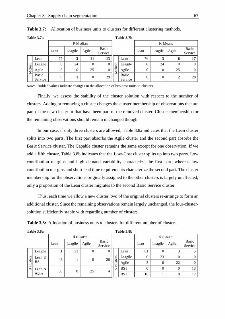
Chapter 3 Supply chain segmentation 67
Table 3.7: Allocation of business units to clusters for different clustering methods.
Table 3.7a Table 3.7b
P-Median
Lean Leagile Agile Basic
Service
Mcl
ust
Lean 75 3 11 13
Leagile 0 24 0 0
Agile 0 0 25 0
Basic
Service 0 1 0 29
K-Means
Lean Leagile Agile Basic
Service
Mcl
ust
Lean 76 3 6 17
Leagile 0 24 0 0
Agile 0 0 25 0
Basic
Service 0 0 2 28
Note: Bolded values indicate changes in the allocation of business units to clusters
Finally, we assess the stability of the cluster solution with respect to the number of
clusters. Adding or removing a cluster changes the cluster membership of observations that are
part of the new cluster or that have been part of the removed cluster. Cluster membership for
the remaining observations should remain unchanged though.
In our case, if only three clusters are allowed, Table 3.8a indicates that the Lean cluster
splits into two parts. The first part absorbs the Agile cluster and the second part absorbs the
Basic Service cluster. The Capable cluster remains the same except for one observation. If we
add a fifth cluster, Table 3.8b indicates that the Low-Cost cluster splits up into two parts. Low
contribution margins and high demand variability characterize the first part, whereas low
contribution margins and short lead time requirements characterize the second part. The cluster
membership for the observations originally assigned to the other clusters is largely unaffected;
only a proportion of the Lean cluster migrates to the second Basic Service cluster.
Thus, each time we allow a new cluster, two of the original clusters re-arrange to form an
additional cluster. Since the remaining observations remain largely unchanged, the four-cluster-
solution sufficiently stable with regarding number of clusters.
Table 3.8: Allocation of business units to clusters for different number of clusters.
Table 3.8a Table 3.8b
4 clusters
Lean Leagile Agile Basic
Service
3 c
lust
ers
Leagile 1 23 0 0
Lean &
BS 43 1 0 26
Lean &
Agile 58 0 25 4
4 clusters
Lean Leagile Agile Basic
Service
5 c
lust
ers
Lean 81 0 3 5
Leagile 0 23 0 0
Agile 3 0 22 0
BS I 0 0 0 13
BS II 18 1 0 12
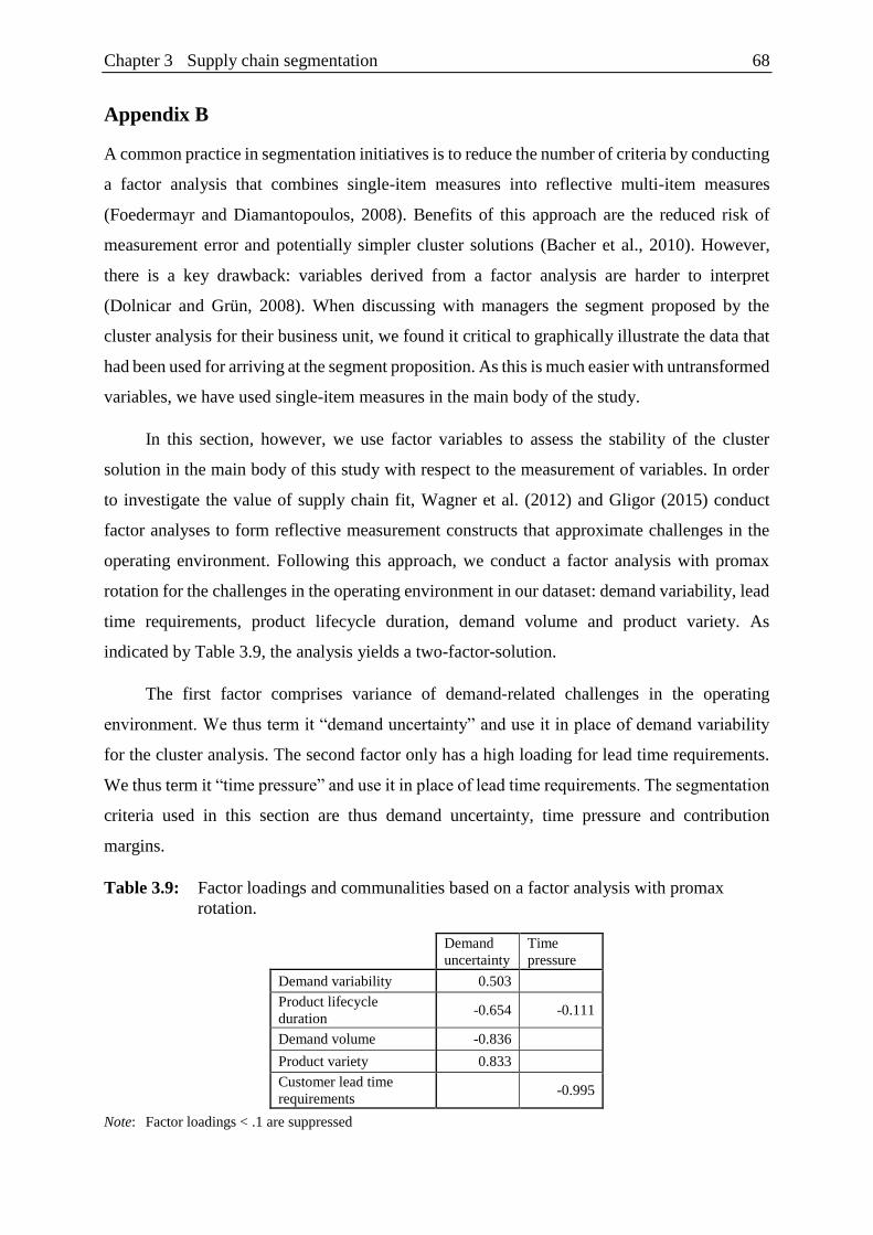
Chapter 3 Supply chain segmentation 68
Appendix B
A common practice in segmentation initiatives is to reduce the number of criteria by conducting
a factor analysis that combines single-item measures into reflective multi-item measures
(Foedermayr and Diamantopoulos, 2008). Benefits of this approach are the reduced risk of
measurement error and potentially simpler cluster solutions (Bacher et al., 2010). However,
there is a key drawback: variables derived from a factor analysis are harder to interpret
(Dolnicar and Grün, 2008). When discussing with managers the segment proposed by the
cluster analysis for their business unit, we found it critical to graphically illustrate the data that
had been used for arriving at the segment proposition. As this is much easier with untransformed
variables, we have used single-item measures in the main body of the study.
In this section, however, we use factor variables to assess the stability of the cluster
solution in the main body of this study with respect to the measurement of variables. In order
to investigate the value of supply chain fit, Wagner et al. (2012) and Gligor (2015) conduct
factor analyses to form reflective measurement constructs that approximate challenges in the
operating environment. Following this approach, we conduct a factor analysis with promax
rotation for the challenges in the operating environment in our dataset: demand variability, lead
time requirements, product lifecycle duration, demand volume and product variety. As
indicated by Table 3.9, the analysis yields a two-factor-solution.
The first factor comprises variance of demand-related challenges in the operating
environment. We thus term it “demand uncertainty” and use it in place of demand variability
for the cluster analysis. The second factor only has a high loading for lead time requirements.
We thus term it “time pressure” and use it in place of lead time requirements. The segmentation
criteria used in this section are thus demand uncertainty, time pressure and contribution
margins.
Table 3.9: Factor loadings and communalities based on a factor analysis with promax
rotation.
Demand
uncertainty
Time
pressure
Demand variability 0.503
Product lifecycle
duration -0.654 -0.111
Demand volume -0.836
Product variety 0.833
Customer lead time
requirements -0.995
Note: Factor loadings < .1 are suppressed
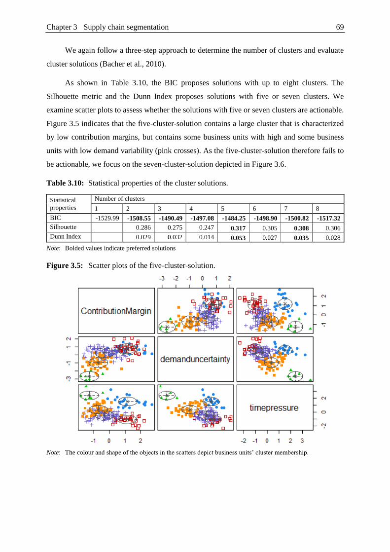
Chapter 3 Supply chain segmentation 69
We again follow a three-step approach to determine the number of clusters and evaluate
cluster solutions (Bacher et al., 2010).
As shown in Table 3.10, the BIC proposes solutions with up to eight clusters. The
Silhouette metric and the Dunn Index proposes solutions with five or seven clusters. We
examine scatter plots to assess whether the solutions with five or seven clusters are actionable.
Figure 3.5 indicates that the five-cluster-solution contains a large cluster that is characterized
by low contribution margins, but contains some business units with high and some business
units with low demand variability (pink crosses). As the five-cluster-solution therefore fails to
be actionable, we focus on the seven-cluster-solution depicted in Figure 3.6.
Table 3.10: Statistical properties of the cluster solutions.
Statistical
properties
Number of clusters
1 2 3 4 5 6 7 8
BIC -1529.99 -1508.55 -1490.49 -1497.08 -1484.25 -1498.90 -1500.82 -1517.32
Silhouette 0.286 0.275 0.247 0.317 0.305 0.308 0.306
Dunn Index 0.029 0.032 0.014 0.053 0.027 0.035 0.028
Note: Bolded values indicate preferred solutions
Figure 3.5: Scatter plots of the five-cluster-solution.
Note: The colour and shape of the objects in the scatters depict business units’ cluster membership.
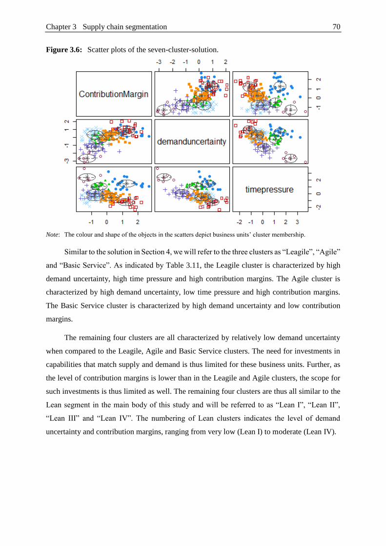
Chapter 3 Supply chain segmentation 70
Figure 3.6: Scatter plots of the seven-cluster-solution.
Note: The colour and shape of the objects in the scatters depict business units’ cluster membership.
Similar to the solution in Section 4, we will refer to the three clusters as “Leagile”, “Agile”
and “Basic Service”. As indicated by Table 3.11, the Leagile cluster is characterized by high
demand uncertainty, high time pressure and high contribution margins. The Agile cluster is
characterized by high demand uncertainty, low time pressure and high contribution margins.
The Basic Service cluster is characterized by high demand uncertainty and low contribution
margins.
The remaining four clusters are all characterized by relatively low demand uncertainty
when compared to the Leagile, Agile and Basic Service clusters. The need for investments in
capabilities that match supply and demand is thus limited for these business units. Further, as
the level of contribution margins is lower than in the Leagile and Agile clusters, the scope for
such investments is thus limited as well. The remaining four clusters are thus all similar to the
Lean segment in the main body of this study and will be referred to as “Lean I”, “Lean II”,
“Lean III” and “Lean IV”. The numbering of Lean clusters indicates the level of demand
uncertainty and contribution margins, ranging from very low (Lean I) to moderate (Lean IV).
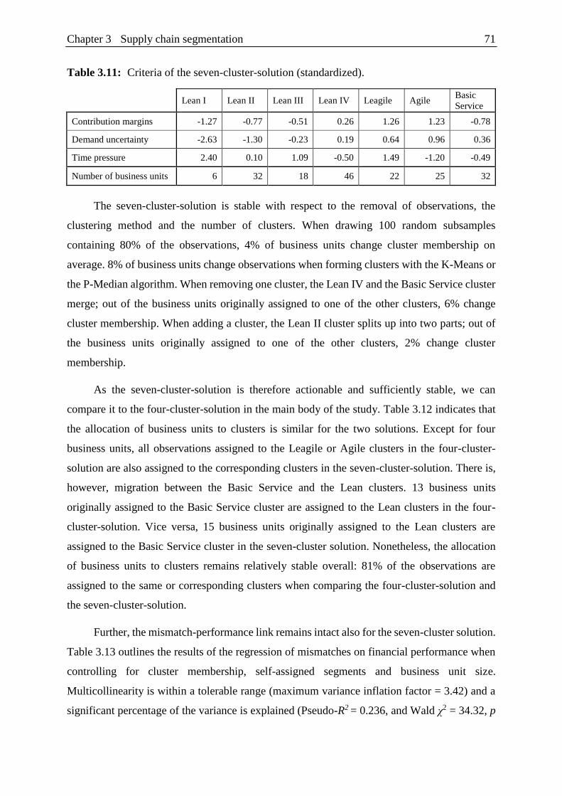
Chapter 3 Supply chain segmentation 71
Table 3.11: Criteria of the seven-cluster-solution (standardized).
Lean I Lean II Lean III Lean IV Leagile Agile Basic
Service
Contribution margins -1.27 -0.77 -0.51 0.26 1.26 1.23 -0.78
Demand uncertainty -2.63 -1.30 -0.23 0.19 0.64 0.96 0.36
Time pressure 2.40 0.10 1.09 -0.50 1.49 -1.20 -0.49
Number of business units 6 32 18 46 22 25 32
The seven-cluster-solution is stable with respect to the removal of observations, the
clustering method and the number of clusters. When drawing 100 random subsamples
containing 80% of the observations, 4% of business units change cluster membership on
average. 8% of business units change observations when forming clusters with the K-Means or
the P-Median algorithm. When removing one cluster, the Lean IV and the Basic Service cluster
merge; out of the business units originally assigned to one of the other clusters, 6% change
cluster membership. When adding a cluster, the Lean II cluster splits up into two parts; out of
the business units originally assigned to one of the other clusters, 2% change cluster
membership.
As the seven-cluster-solution is therefore actionable and sufficiently stable, we can
compare it to the four-cluster-solution in the main body of the study. Table 3.12 indicates that
the allocation of business units to clusters is similar for the two solutions. Except for four
business units, all observations assigned to the Leagile or Agile clusters in the four-cluster-
solution are also assigned to the corresponding clusters in the seven-cluster-solution. There is,
however, migration between the Basic Service and the Lean clusters. 13 business units
originally assigned to the Basic Service cluster are assigned to the Lean clusters in the four-
cluster-solution. Vice versa, 15 business units originally assigned to the Lean clusters are
assigned to the Basic Service cluster in the seven-cluster solution. Nonetheless, the allocation
of business units to clusters remains relatively stable overall: 81% of the observations are
assigned to the same or corresponding clusters when comparing the four-cluster-solution and
the seven-cluster-solution.
Further, the mismatch-performance link remains intact also for the seven-cluster solution.
Table 3.13 outlines the results of the regression of mismatches on financial performance when
controlling for cluster membership, self-assigned segments and business unit size.
Multicollinearity is within a tolerable range (maximum variance inflation factor = 3.42) and a
significant percentage of the variance is explained (Pseudo-R2 = 0.236, and Wald χ2 = 34.32, p

Chapter 3 Supply chain segmentation 72
< 0.001). The link between mismatches and financial performance is significant and negative
(β1 = -0.067, p < 0.01), indicating that Hypothesis 1 also supported for the seven-cluster-
solution.
In summary, the interpretation of clusters, the allocation of business unit to clusters, and
the performance implications of segment-environment mismatches are similar for the four-
cluster-solution in Section 4 and the seven-cluster-solution in the appendix. The solutions are
therefore sufficiently stable regarding changes in the measurement of segmentation criteria.
Table 3.12: Allocation of business units to clusters for the four-cluster-solution and the seven-
cluster-solution.
Lean I Lean II Lean III Lean IV Leagile Agile Basic
Service
Lean 5 10 42 29 0 1 15
Leagile 0 2 0 0 22 0 0
Agile 0 0 2 0 0 23 0
Basic Service 1 6 2 3 0 1 17
Note: Bolded values indicate changes in the allocation of business units to clusters
Table 3.13: Regression results with p-values and bias-corrected confidence intervals.
Independent variables
Dependent variable
Financial
Performance
Financial
Performance
Financial
Performance
Financial
Performance
Cluster Lean I -0.044
[-0.104, 0.020]
-0.055
[-0.116, 0.003]
-0.067
[-0.159, 0.012]
-0.074
[-0.164, 0.004]
Cluster Lean II -0.034
[-0.061, 0.013]
-0.041*
[-0.067, -0.005]
-0.033
[-0.059, 0.010]
-0.038*
[-0.064, -0.002]
Cluster Lean III -0.031
[-0.114, 0.009]
-0.027
[-0.115, 0.016]
0.042*
[-0.125, -0.002]
-0.039
[-0.124, 0.005]
Cluster Leagile -0.016
[-0.056, 0.017]
-0.047**
[-0.078, -0.016]
-0.009
[-0.046, 0.020]
-0.038*
[-0.067, -0.007]
Cluster Agile -0.011
[-0.053, 0.022]
-0.026
[-0.066, 0.005]
-0.007
[-0.051, 0.022]
-0.021
[-0.063, 0.008]
Self-assigned Leagile 0.012
[-0.022, 0.067]
0.060*
[0.006, 0.113]
0.018
[-0.017, 0.067]
0.062*
[0.011, 0.112]
Self-assigned Agile -0.007
[-0.057, 0.047]
0.047*
[0.006, 0.097]
-0.005
[-0.050, 0.048]
0.043*
[0.001, 0.089]
Business unit size 0.026***
[0.010, 0.041]
0.023**
[0.010, 0.040]
Mismatches -0.074**
[-0.118, -0.023]
-0.067**
[-0.108, -0.022]
Wald χ2 10.93 21.13** 24.17** 34.32***
ICC 0.389*** 0.389*** 0.389*** 0.389***
Pseudo-R2 0.058 0.113 0.183 0.236
Note: * p < 0.05, ** p < 0.01, *** p < 0.001 (two-tailed).

Chapter 4 Performance outcomes of responsiveness 73
Chapter 4 Performance outcomes of responsiveness:
When should supply chains be fast?
Co-authors:
Moritz Fleischmann
Chair of Logistics and Supply Chain Management, Business School, University of
Mannheim, Germany
Christoph Bode
Endowed Chair of Procurement, Business School, University of Mannheim, Germany
Abstract
Responsiveness is considered a “basis of competition” attribute of supply chain performance
(APICS, 2016). Nonetheless, there remains ambiguity under which conditions a supply chain
that is fast enough to fulfil customers’ lead time requirements constitutes competitive
advantage. We examine the benefits and costs associated with supply chain responsiveness
using secondary data from a leading chemicals manufacturer. Our results indicate that
responsiveness can improve financial performance in two distinct ways: either by matching
supply and demand or by decreasing supply-chain-related costs depending on the characteristics
of the products that are being sold. Based on these findings, this study aims to contribute to
supply chain strategy literature by providing managers guidance on when their supply chains
should be fast.
Chapter 4 Performance outcomes of responsiveness 74
Introduction
The Cambridge Dictionary defines responsiveness as “how quickly and well a person or
organization reacts to something” (Cambridge Dictionary, 2016). In supply chain management,
responsiveness describes the ability of a supply chain to fulfil orders within a time frame that
is acceptable to the customer (Chen et al., 2004; Holweg, 2005). It is considered a “basis of
competition” attribute of supply chain performance that has been linked to higher revenues
(APICS, 2016; Elgazzar et al., 2012). So why have empirical studies failed to find a link
between shorter lead times – a popular measure of responsiveness – and financial performance
(Croom et al., 2007; Droge et al., 2004)? The answer is simple: there are clear limits to time-
based competition, as the value of reducing lead times to better meet customer requirements is
often too low to warrant higher costs (Blackburn, 2012). Cost premiums associated with shorter
lead times explain why some companies deliberately extend lead times through practices such
as “slow steaming” or offshoring production (Cariou, 2011; Kinkel and Maloca, 2009). As a
more responsive supply chain is thus not only a potential source of value, but may also be a
source of higher costs, managers need to carefully consider both the benefits and costs of shorter
lead times. Our goal is therefore to support managers confronted with lead-time-related
decisions by analysing the performance outcomes of responsiveness. In doing so, we aim to
answer the following research question: when should supply chains be fast?
Assessing the performance outcomes of responsiveness is challenging because of the
many factors that influence the benefits and costs associated with shorter lead times. A simple
yet powerful framework for assessing responsiveness has been proposed by Fisher (1997):
companies selling innovative products will perform best with a responsive supply chain,
whereas companies selling functional products should instead adopt a supply chain that focuses
on efficiency. Fisher’s framework thus suggests that companies selling innovative products
should make lead time reductions a competitive priority, whereas companies selling functional
products should not.
Several studies have found support for Fisher’s framework regarding the benefits of
shorter lead times. Based on a simulation study, Blackburn (2012) finds that the marginal value
of lead time reductions is low for functional products. Using real options theory, de Treville et
al. (2014a) and de Treville et al. (2014b) highlight that the marginal value of lead time
reductions is much higher for innovative products with characteristics such as high demand
variability, demand clustering, tender loss risk or low salvage values. However, while these
studies provide valuable insights by highlighting the context-dependency of the benefits of
Chapter 4 Performance outcomes of responsiveness 75
shorter lead times, they rely on overly simplistic assumptions regarding the costs that lead time
reductions entail.
Existing models analysing the benefits of shorter lead times assume that lead time
compression entails a cost premium (Blackburn, 2012; de Treville et al., 2014a; de Treville et
al., 2014b). Jian et al. (2015) model the benefits and costs of shorter lead times, assuming that
costs related to lead time compression are a linear function of lead times.6 Many levers for
reducing lead times like airfreight or shipping less-than-full truckloads are indeed costly.
However, there are also levers that reduce supply-chain-related costs by cutting lead times.
Lean practice bundles, for instance, are associated with both lead time and cost reductions
(Mackelprang and Nair, 2010; Narasimhan et al., 2006; Shah and Ward, 2003). The classic
assumption that responsiveness entails a cost premium is thus overly simplistic and needs to be
challenged. Apart from examining the context-dependency of the benefits of responsiveness,
we therefore also analyse the conditions under which shorter lead times are associated with
higher or lower costs. Based on the findings of our empirical analysis, this article contributes
to the supply chain strategy literature by offering managers guidance as to when they should
make responsiveness a competitive priority.
The remainder of the paper is organized as follows. Section 2 provides the theoretical
background for deriving hypotheses. Section 3 describes the dataset and specifies the measures
used in this study. Section 4 introduces the methodology. In Section 5 the results of the analysis
are outlined; the implications for managers and researchers are presented in Section 6. Finally,
Section 7 concludes with the limitations of our work and suggestions for future research.
Conceptual model
2.1 The responsiveness-performance link
Several empirical studies have analysed the link between responsiveness and financial
performance, but they found no empirical support for a strong, direct relationship (Croom et
al., 2007; Droge et al., 2004). Two reasons are likely: (1) measuring responsiveness purely
based on the length of lead times may not be appropriate and (2) there are opposing intermediate
performance outcomes (mediation) that need to be accounted for.
6 According to Jian et al. (2015), lead time compression incurs crashing costs which comprise of expenditures on
equipment improvement, information technology, order expedite, special shipping and handling.
Chapter 4 Performance outcomes of responsiveness 76
2.1.1 Measuring responsiveness
Shorter lead times are assumed to positively affect companies’ top-line performance (Elgazzar
et al., 2012). The underlying reasoning is that if a company’s lead times exceed its customers’
willingness to wait for a product, customers will buy elsewhere and the company will in turn
loose sales. Both theoretical and empirical models have thus used different measures of lead
times to assess the value of responsiveness (Blackburn, 2012; de Treville et al., 2014a; Droge
et al., 2004). The SCOR framework – a “standard” performance management model for
operational performance (de Leeuw and van den Berg, 2011) – also uses end-to-end cycle times
to measure supply chain responsiveness. Order fulfilment lead times (i.e., the time between
order placement and the actual delivery date) indeed measure how long the customer needs to
wait for the order to arrive. However, whether a supply chain is perceived as “fast” or “slow”
also depends on the lead time requirement of the customer.
To illustrate this point, consider two examples. First, let us assume the case of a custom-
made product. Customers grant 30 days until delivery, as this product cannot easily be obtained
from a different supplier. In this example, a delivery after 29 days would be perceived as fast
enough and delivery after 33 days would be perceived as too slow. Second, consider an off-the-
shelf product that the customer expects to receive within 5 days, as it can be sourced from
different suppliers. In this second example, a delivery after 4 days would be perceived as fast
enough and delivery after 7 days would be perceived as too slow. The ability of shorter lead
times to improve financial performance by avoiding lost sales thus depends on the lead time
requirement of customers (i.e., the time between order placement and requested delivery date).
When examining the ability of shorter lead times to improve financial performance by
avoiding lost sales, we thus need to assess order fulfilment lead times relative to the lead time
requirements of customers. Accordingly, we measure supply chain responsiveness as the
difference between the customer lead time requirement and the order fulfilment lead time. In
the first example above, the supply chain that is perceived as fast enough would have a
responsiveness of 1, whereas the too slow supply chain would have a responsiveness of -3 (in
the second example, the respective values are 1 and -2). By incorporating both customer lead
time requirements and order fulfilment lead times in our measure of responsiveness, we aim to
generate more accurate insights on the performance outcomes of shorter lead times and time-
based competition.
Chapter 4 Performance outcomes of responsiveness 77
2.1.2 Intermediate performance outcomes of responsiveness
There are two points of view on the performance outcomes of responsiveness in the literature.
According to the first, responsiveness has a direct and positive effect on financial performance.
This view is reflected by the SCOR model which classifies responsiveness as one of the key
performance attributes for “measur[ing] how successful [a supply chain] is in achieving its
desired positioning within the competitive market space” (APICS, 2016). Responsiveness has
also been linked to higher revenues in the conceptual literature (Elgazzar et al., 2012). However,
empirical studies examining the direct link between shorter lead times and financial
performance failed to find a significant relationship (Croom et al., 2007; Droge et al., 2004).
According to the second, a set of intermediate performance outcomes mediates the effect
of responsiveness on financial performance. On the one hand, responsiveness helps to match
supply and demand and thereby prevents lost sales. On the other hand, responsiveness is often
associated with higher supply-chain-related costs. The notion of opposing intermediate
performance outcomes may explain why previous studies failed to establish a direct link
between responsiveness and financial performance: in many cases the benefits of better meeting
customers’ lead time requirements do not outweigh the associated costs.
Proponents of the latter perspective include Fisher (1997), who recognizes that supply
chains have two functions: (1) to match supply and demand (“market mediation function”) and
(2) to efficiently provide products to customers (“physical function”). According to Fisher,
responsiveness is a lever for improving the market mediation function, although this often
comes at the expense of lower physical efficiency. Similarly, theoretical models on the value
of shorter lead times measure the benefits of a faster supply chain based on avoided demand
and supply mismatches (Blackburn, 2012; de Treville et al., 2014a; de Treville et al., 2014b).
Following this line of thought, this study asks how responsiveness is linked to financial
performance via the match between supply and demand (market mediation function), as well
as supply-chain-related costs (physical function). The examined relationships are illustrated in
Figure 4.1.

Chapter 4 Performance outcomes of responsiveness 78
Figure 4.1: Conceptual framework (Level 1 and Level 2 are explained in Section 3).
2.2 Responsiveness and the market mediation function
2.2.1 Direct effects
Responsiveness helps to avoid lost sales by matching supply and demand. An indicator of the
match between supply and demand is reliability which reflects the proportion of orders where
customer expectations have been met with respect to time (on time), quantity (in full) and
condition (in quality) (APICS, 2016; Shepherd and Günter, 2006). An order is considered on
time, if it arrives within the delivery window specified by the customer. As responsiveness is
thus a key determinant of the on time performance, we hypothesize a positive relationship
between responsiveness and reliability:
Hypothesis 1: There is a positive relationship between responsiveness and reliability.
Supply chain reliability has major implications for the financial performance of a
company. A failure to deliver as promised may at best result in a negative customer experience
with no adverse financial effects. It is more likely, however, that a failure to deliver as promised
will result in penalty payments, lost sales, and foregone contribution margins (Langenberg et
al., 2012). A large scale supply chain disruption or recurring unreliability will damage customer
relationships and eventually result in disappointed customers leaving for good (Craighead et
al., 2007; Habermann et al., 2015; Hendricks and Singhal, 2005). Hence, we posit:
Hypothesis 2: There is a positive relationship between reliability and financial
performance.

Chapter 4 Performance outcomes of responsiveness 79
2.2.2 Moderating effects
According to Fisher (1997), being responsive is more important for “innovative” products than
for “functional” products. With respect to their influence on the importance of responsiveness,
characteristics of innovative products can be grouped into two categories: challenges in the
operating environment and factors influencing the value of matching supply and demand. The
former make it more difficult to match supply and demand and thereby increase the need for
responsiveness. The latter affect the cost of overage and underage and therefore the value of
matching supply and demand.
Challenges in the operating environment inhibit the ability to match supply and demand,
ceteris paribus. Frameworks for supply chain or manufacturing strategies typically comprise
demand-related and time-related challenges. According to Fisher (1997), challenges in the
operating environment comprise different causes of demand uncertainty (short lifecycles,
forecast error and high product variety) as well as the time granted by customers to fulfil orders.
The same is true for the DWV3 framework by Christopher et al. (2009) which also considers
different sources of demand uncertainty (demand variability and volume, product variety and
the product lifecycle) as well as the customer lead time requirement. Olhager (2003) explicitly
maps challenges of the operating environment along a time-related and a demand-related
dimension. Following these frameworks, our study evaluates how demand variability – which
we use as a proxy for demand-related challenges – and customer lead time requirements
moderate the relationship between responsiveness and reliability.
In environments characterized by recurring demand peaks, the ability to react to customer
needs in a timely manner can be a valuable buffer that allows on time delivery nonetheless.
When demand is stable, this buffer will not be used and thus does not contribute to reliability.
Similarly, if customers demand short lead times, there is less time to react to unexpected
changes in demand. Consequently, capabilities that allow supply chains to react quickly will
have a larger effect than in an environment where most orders are delivered on time anyways.
We thus expect the need for responsiveness to be higher in operating environments
characterized by high demand variability and short customer lead time requirements.
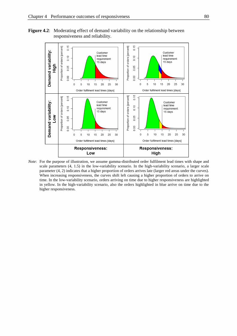
Chapter 4 Performance outcomes of responsiveness 80
Figure 4.2: Moderating effect of demand variability on the relationship between
responsiveness and reliability.
Note: For the purpose of illustration, we assume gamma-distributed order fulfilment lead times with shape and
scale parameters (4, 1.5) in the low-variability scenario. In the high-variability scenario, a larger scale
parameter (4, 2) indicates that a higher proportion of orders arrives late (larger red areas under the curves).
When increasing responsiveness, the curves shift left causing a higher proportion of orders to arrive on
time. In the low-variability scenario, orders arriving on time due to higher responsiveness are highlighted
in yellow. In the high-variability scenario, also the orders highlighted in blue arrive on time due to the
higher responsiveness.
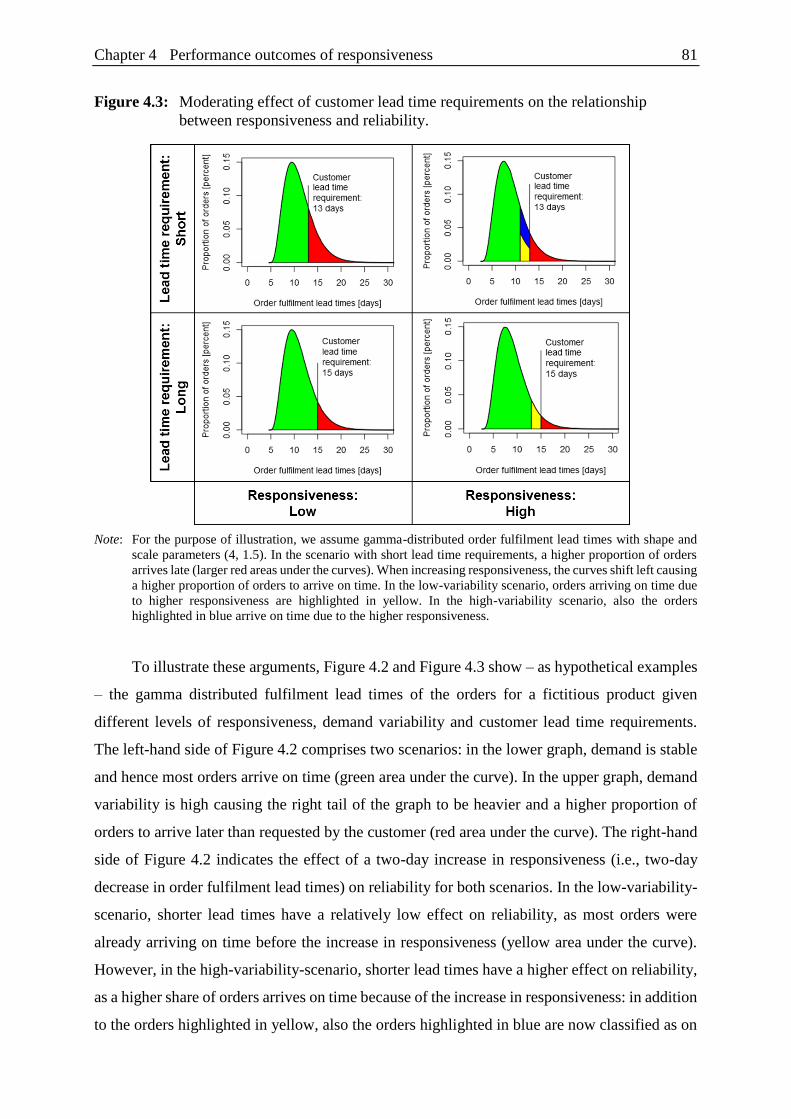
Chapter 4 Performance outcomes of responsiveness 81
Figure 4.3: Moderating effect of customer lead time requirements on the relationship
between responsiveness and reliability.
Note: For the purpose of illustration, we assume gamma-distributed order fulfilment lead times with shape and
scale parameters (4, 1.5). In the scenario with short lead time requirements, a higher proportion of orders
arrives late (larger red areas under the curves). When increasing responsiveness, the curves shift left causing
a higher proportion of orders to arrive on time. In the low-variability scenario, orders arriving on time due
to higher responsiveness are highlighted in yellow. In the high-variability scenario, also the orders
highlighted in blue arrive on time due to the higher responsiveness.
To illustrate these arguments, Figure 4.2 and Figure 4.3 show – as hypothetical examples
– the gamma distributed fulfilment lead times of the orders for a fictitious product given
different levels of responsiveness, demand variability and customer lead time requirements.
The left-hand side of Figure 4.2 comprises two scenarios: in the lower graph, demand is stable
and hence most orders arrive on time (green area under the curve). In the upper graph, demand
variability is high causing the right tail of the graph to be heavier and a higher proportion of
orders to arrive later than requested by the customer (red area under the curve). The right-hand
side of Figure 4.2 indicates the effect of a two-day increase in responsiveness (i.e., two-day
decrease in order fulfilment lead times) on reliability for both scenarios. In the low-variability-
scenario, shorter lead times have a relatively low effect on reliability, as most orders were
already arriving on time before the increase in responsiveness (yellow area under the curve).
However, in the high-variability-scenario, shorter lead times have a higher effect on reliability,
as a higher share of orders arrives on time because of the increase in responsiveness: in addition
to the orders highlighted in yellow, also the orders highlighted in blue are now classified as on
Chapter 4 Performance outcomes of responsiveness 82
time instead of delayed. Figure 4.2 therefore provides further support for our assumption that
the effect of responsiveness on reliability increases with demand variability. Figure 4.3
indicates that short customer lead times requirements have a similar moderating effect. A
comparison of the graphs on the right-hand side reveals that responsiveness has a stronger effect
on reliability if lead time requirements are short; the increase of the effect is again marked in
blue.
In summary, we expect high demand variability and short customer lead time
requirements to positively moderate the relationship between responsiveness and reliability:
Hypothesis 3: The positive relationship between responsiveness and reliability is
stronger when the level of challenges in the operating environment is
high (high demand variability and short customer lead time
requirements) than when it is low (low demand variability and long
customer lead time requirements).
Challenges in the operating environment make it harder to match supply and demand,
ceteris paribus. In environments characterized by uncertainty and time pressure, supply chain
responsiveness is particularly important for preventing supply-and-demand mismatches. Yet,
before investing in responsiveness to cope with a challenging operating environment, managers
need to ensure that the benefits of responsiveness clearly outweigh the associated costs. For this
purpose, contribution margins have to be considered, because they influence the effect of lost
sales on the bottom line (Randall et al., 2003). If contribution margins are high, managers
should be willing to incur higher market mediation costs, since the cost of lost sales is also
higher (Hendricks and Singhal, 2003). In contrast, if contributions margins are low, the
incentive to match supply and demand will also be lower. Hence, contribution margins are
decisive for the willingness to invest in capabilities that help to match supply and demand such
as responsiveness:
Hypothesis 4: The positive relationship between reliability and financial performance
is stronger when contribution margins are high than when they are low.
2.3 Responsiveness and the physical function
The relationship between responsiveness and supply-chain-related costs is also subject to
moderating factors. Challenges in the operating environment are critical for determining
whether responsiveness leads to higher or lower supply-chain-related costs.
Chapter 4 Performance outcomes of responsiveness 83
Several studies have linked process improvements and waste reduction (lean) initiatives
to both shorter lead times and lower supply-chain-related costs (Mackelprang and Nair, 2010;
Narasimhan et al., 2006; Shah and Ward, 2003). The concept of just-in-time production, for
instance, includes practices such as the elimination of bottlenecks and the reduction of batch
sizes which aim to minimize work-in-progress inventory by reducing throughput times
(Sugimori et al., 1977). Yet a prerequisite for just-in-time production is a level production
schedule which is hard to achieve when demand is variable. Practices that cut lead times in
order to achieve a higher cost efficiency therefore fail to reap the expected benefits in
environments characterized by dynamism or technological turbulence (Azadegan et al., 2013;
Chavez et al., 2015). It is also more challenging to improve the efficiency and responsiveness
of processes in environments characterized by instability and uncertainty, as such environments
inhibit learning (Browning and Heath, 2009). Consequently, we only expect responsiveness to
be associated with lower supply-chain-related costs in an operating environment characterized
by stable demand and customers granting sufficient time to react to uncertainties.
In an environment characterized by volatile demand or time pressure, we expect
responsiveness to be associated with higher supply-chain-related costs. Companies may build
inventory buffers to remain responsive to customer orders even when demand is volatile. They
may also resort to costly options for decreasing delivery lead times such as less-than-full
truckload shipments or airfreight when under time pressure. Responsiveness therefore entails a
cost premium if it is used as a market mediation capability that mitigates the adverse effects of
challenges in the operating environment on reliability.
This study focusses on two types of supply-chain-related costs: inventory and logistics
costs.7 These cost types are not only assumed to be affected by process improvements and
waste reduction initiatives (Goldsby and Martichenko, 2005; Mackelprang and Nair, 2010), but
also by costly enablers of responsiveness such as inventory buffers and airfreight. Accordingly,
we posit:
Hypothesis 5: The relationship between responsiveness and supply-chain-related costs
(inventory and logistics costs) is
(a) positive when the level of challenges in the operating environment is
high (high demand variability and short customer lead time
requirements).
7 Inventory is measured by days in inventory. Logistics costs comprise of all costs related to freight, distribution,
warehousing order management and materials management as a percentage of sales.
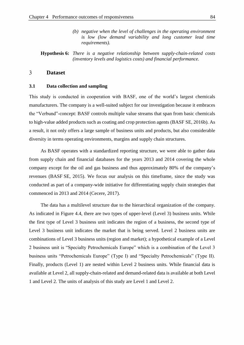
Chapter 4 Performance outcomes of responsiveness 84
(b) negative when the level of challenges in the operating environment
is low (low demand variability and long customer lead time
requirements).
Hypothesis 6: There is a negative relationship between supply-chain-related costs
(inventory levels and logistics costs) and financial performance.
Dataset
3.1 Data collection and sampling
This study is conducted in cooperation with BASF, one of the world’s largest chemicals
manufacturers. The company is a well-suited subject for our investigation because it embraces
the “Verbund”-concept: BASF controls multiple value streams that span from basic chemicals
to high-value added products such as coating and crop protection agents (BASF SE, 2016b). As
a result, it not only offers a large sample of business units and products, but also considerable
diversity in terms operating environments, margins and supply chain structures.
As BASF operates with a standardized reporting structure, we were able to gather data
from supply chain and financial databases for the years 2013 and 2014 covering the whole
company except for the oil and gas business and thus approximately 80% of the company’s
revenues (BASF SE, 2015). We focus our analysis on this timeframe, since the study was
conducted as part of a company-wide initiative for differentiating supply chain strategies that
commenced in 2013 and 2014 (Cecere, 2017).
The data has a multilevel structure due to the hierarchical organization of the company.
As indicated in Figure 4.4, there are two types of upper-level (Level 3) business units. While
the first type of Level 3 business unit indicates the region of a business, the second type of
Level 3 business unit indicates the market that is being served. Level 2 business units are
combinations of Level 3 business units (region and market); a hypothetical example of a Level
2 business unit is “Specialty Petrochemicals Europe” which is a combination of the Level 3
business units “Petrochemicals Europe” (Type I) and “Specialty Petrochemicals” (Type II).
Finally, products (Level 1) are nested within Level 2 business units. While financial data is
available at Level 2, all supply-chain-related and demand-related data is available at both Level
1 and Level 2. The units of analysis of this study are Level 1 and Level 2.
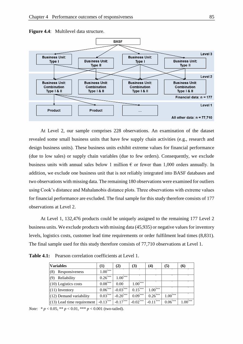
Chapter 4 Performance outcomes of responsiveness 85
Figure 4.4: Multilevel data structure.
At Level 2, our sample comprises 228 observations. An examination of the dataset
revealed some small business units that have few supply chain activities (e.g., research and
design business units). These business units exhibit extreme values for financial performance
(due to low sales) or supply chain variables (due to few orders). Consequently, we exclude
business units with annual sales below 1 million € or fewer than 1,000 orders annually. In
addition, we exclude one business unit that is not reliably integrated into BASF databases and
two observations with missing data. The remaining 180 observations were examined for outliers
using Cook’s distance and Mahalanobis distance plots. Three observations with extreme values
for financial performance are excluded. The final sample for this study therefore consists of 177
observations at Level 2.
At Level 1, 132,476 products could be uniquely assigned to the remaining 177 Level 2
business units. We exclude products with missing data (45,935) or negative values for inventory
levels, logistics costs, customer lead time requirements or order fulfilment lead times (8,831).
The final sample used for this study therefore consists of 77,710 observations at Level 1.
Table 4.1: Pearson correlation coefficients at Level 1.
Variables (1) (2) (3) (4) (5) (6)
(8) Responsiveness 1.00 ***
(9) Reliability 0.26 *** 1.00 ***
(10) Logistics costs 0.08 *** 0.00 1.00 ***
(11) Inventory 0.06 *** -0.03 *** 0.15 *** 1.00 ***
(12) Demand variability 0.03 *** -0.20 *** 0.09 *** 0.26 *** 1.00 ***
(13) Lead time requirement -0.13 *** -0.17 *** -0.02 *** -0.11 *** 0.06 *** 1.00 ***
Note: * p < 0.05, ** p < 0.01, *** p < 0.001 (two-tailed).
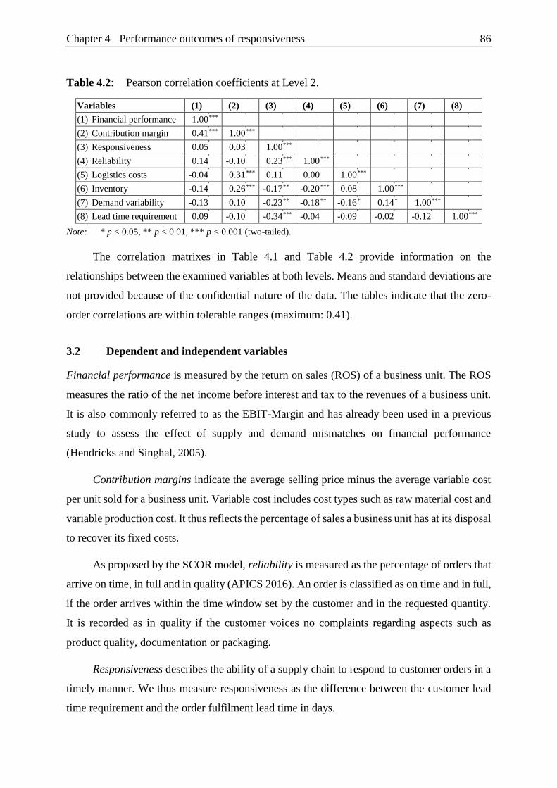
Chapter 4 Performance outcomes of responsiveness 86
Table 4.2: Pearson correlation coefficients at Level 2.
Variables (1) (2) (3) (4) (5) (6) (7) (8)
(1) Financial performance 1.00 ***
(2) Contribution margin 0.41 *** 1.00 ***
(3) Responsiveness 0.05 0.03 1.00 ***
(4) Reliability 0.14 -0.10 0.23 *** 1.00 ***
(5) Logistics costs -0.04 0.31 *** 0.11 0.00 1.00 ***
(6) Inventory -0.14 0.26 *** -0.17 ** -0.20 *** 0.08 1.00 ***
(7) Demand variability -0.13 0.10 -0.23 ** -0.18 ** -0.16 * 0.14 * 1.00 ***
(8) Lead time requirement 0.09 -0.10 -0.34 *** -0.04 -0.09 -0.02 -0.12 1.00 ***
Note: * p < 0.05, ** p < 0.01, *** p < 0.001 (two-tailed).
The correlation matrixes in Table 4.1 and Table 4.2 provide information on the
relationships between the examined variables at both levels. Means and standard deviations are
not provided because of the confidential nature of the data. The tables indicate that the zero-
order correlations are within tolerable ranges (maximum: 0.41).
3.2 Dependent and independent variables
Financial performance is measured by the return on sales (ROS) of a business unit. The ROS
measures the ratio of the net income before interest and tax to the revenues of a business unit.
It is also commonly referred to as the EBIT-Margin and has already been used in a previous
study to assess the effect of supply and demand mismatches on financial performance
(Hendricks and Singhal, 2005).
Contribution margins indicate the average selling price minus the average variable cost
per unit sold for a business unit. Variable cost includes cost types such as raw material cost and
variable production cost. It thus reflects the percentage of sales a business unit has at its disposal
to recover its fixed costs.
As proposed by the SCOR model, reliability is measured as the percentage of orders that
arrive on time, in full and in quality (APICS 2016). An order is classified as on time and in full,
if the order arrives within the time window set by the customer and in the requested quantity.
It is recorded as in quality if the customer voices no complaints regarding aspects such as
product quality, documentation or packaging.
Responsiveness describes the ability of a supply chain to respond to customer orders in a
timely manner. We thus measure responsiveness as the difference between the customer lead
time requirement and the order fulfilment lead time in days.
Chapter 4 Performance outcomes of responsiveness 87
As demand uncertainty is hard to measure with archival data, we use demand variability
as a proxy. Demand variability has been suggested as an appropriate measure of demand-related
challenges in the operating environment, since it captures both expected and unexpected
changes in demand (Aitken et al., 2005). We measure it as the coefficient of variation of weekly
sales (Christopher et al. 2009).
The customer lead time requirement is measured by the average number of days
customers grant between the initial order entry and the requested delivery date.
Inventory levels are measured by days in inventory (DIV) which indicates how long it
takes the business unit to turn its inventory into sales. Logistics costs capture all costs related
to freight, distribution, warehousing, order management and materials management as a
percentage of sales.
The variables for responsiveness, demand variability, customer lead time requirements,
inventory levels, and logistics costs are highly skewed. To reduce the influence of extreme
values on parameter estimates, we have transformed these variables. For responsiveness, we
employ the inverse hyperbolic sine transformation for responsiveness because it reduces the
skewness of variables that comprise both positive and non-positive values (Burbidge et al.,
1988). For demand variability, customer lead time requirements, inventory levels and logistics
costs, we use the natural logarithm, because these variables are strictly positive. To render the
scales of the transformed variables more comparable, they are also standardized. All other
variables (financial performance, contribution margins and reliability) are centered at the grand
mean to ease the interpretation of interaction effects.
3.3 Control variables
The customer lead time requirement is included as a control variable when assessing the
relationship between responsiveness and financial performance. On the one hand, long
customer lead time requirements indicate that products are more difficult to deliver or produce.
On the other hand, long customer lead time requirements also indicate that the business unit has
a unique selling proposition which increases customers’ willing to wait. As a consequence,
Table 4.2 shows that the length of customer lead time requirements is negatively correlated
with responsiveness and positively correlated with financial performance.
Finally, it is likely that industry-specific effects have an impact on the examined
performance attributes (Bozarth et al., 2009). Level 2 business units nested within a Level 3

Chapter 4 Performance outcomes of responsiveness 88
business unit are likely to be similar in ways that are otherwise not explicitly accounted for by
our models. As demonstrated in Section 3.1, the Level 3 business unit “Petrochemicals Europe”
for instance contains two Level 2 business units that produce different types of petrochemicals
(standard and specialty petrochemicals). These two business units that operate in the same
industry are likely to have similar competitive and operating environments. The multilevel
models we use for our analysis contain random intercepts to account for similarities of Level 2
business units nested within a Level 3 business unit regarding the examined performance
attributes. They thus implicitly control for industry-specific effects. As will be demonstrated in
the next section, random intercepts explain between 16.6% and 59.8% of the variance in our
models.
Methodology
As indicated by Figure 4.1, we test the hypothesized relationships at two levels. First, we
examine all hypothesized relationships at Level 2. Since financial data is available at that level,
we estimate the direct, indirect and total effects of responsiveness on financial performance.
Second, we analyse the relationships that do not require financial data at Level 1. The goal is
to generate additional insights, as the sample size at Level 1 (n = 77,710) is much higher than
at Level 2 (n = 177).
4.1 Analysis at Level 2
4.1.1 Model description
Due to the multilevel structure of our data, we cannot make inferences from an ordinary
structural equation model, as this would violate the assumption of independent observations
(Hofmann, 1997). In order to analyse the effects of predictors at Level 2, we need to account
for the fact that observations at this level are nested within Level 3 business units. We thus
assess the relationships at Level 2 using a multilevel structural equation model (gsem command
in Stata 14).
The model allows the intercept to vary according to Level 3 business units (Steele and
Goldstein, 2006). Level 2 observations can be attributed to two types of Level 3 observations
(Type I or Type II). Ideally, we would estimate a crossed model that controls for both types of
Level 3 observations (Snijders, 2011). However, there is only one Level 2 observation per
combination of Level 3 observations (e.g., for “Petrochemicals Europe” and “Specialty
Petrochemicals” there is only one Level 2 observation “Specialty Petrochemicals Europe”). As

Chapter 4 Performance outcomes of responsiveness 89
a consequence, a crossed model would be underidentified. We thus estimated the model twice,
once with random intercepts for Level 3 observations of Type I (regions such as
“Petrochemicals Europe”) and once with random intercepts for Level 3 observations of Type II
(markets such as “Specialty Petrochemicals”). The parameter estimates are similar, but a higher
percentage of the variance was explained by the random intercepts in the former model.8 We
thus report the results of the model with random intercepts for Level 3 observations of Type I
in Table 4.3 and Table 4.4.
8 The percentage of variance explained by random intercepts is measured by the intraclass correlation coefficient
(Firebaugh, 1978).

Chapter 4 Performance outcomes of responsiveness 90
Table 4.3: Results at Level 2
for financial performance.
Table 4.4: Results at Level 2
for intermediate performance outcomes.
Independent variables Dependent variable
Independent variables Dependent variables
Financial performance Reliability Inventory Logistics costs
Reliability 0.093**
[0.040, 0.145] Customer lead time
requirement
0.015
[-0.027, 0.039]
-0.064
[-0.195, 0.039]
-0.057
[-0.210, 0.101]
Responsiveness 0.003
[-0.008, 0.011] Demand variability
-0.026**
[-0.045, -0.010]
0.072
[-0.075, 0.228]
-0.057
[-0.183, 0.050]
Inventory -0.020**
[-0.033, -0.011] Responsiveness
0.048***
[0.029, 0.077]
-0.218***
[-0.342, -0.094]
0.107
[-0.028, 0.243]
Logistics Costs -0.016***
[-0.024, -0.006] Cust. lead time requirement ×
Responsiveness
-0.016*
[-0.035, -0.002]
-0.139**
[-0.235, -0.050]
-0.061
[-0.154, 0.039]
Customer lead time
requirement
0.019***
[0.010, 0.029] Demand variability ×
Responsiveness
0.012
[-0.007, 0.033]
-0.020
[-0.140, 0.088]
-0.105
[-0.221, 0.017]
Contribution margins 0.374***
[0.280, 0.444]
Contribution margins ×
Reliability
0.618***
[0.264, 0.910]
Wald χ2 87.01*** Wald χ
2 34.53*** 16.46** 10.38
ICC 0.326*** ICC 0.458*** 0.200*** 0.598***
Pseudo-R2 0.315 Pseudo-R
2 0.178 0.077 0.075
Type of analysis Structural equation model Type of analysis Structural equation
model
Structural equation
model
Structural equation
model
Note: * p < 0.05, ** p < 0.01, *** p < 0.001 (two-tailed). Bias-corrected confidence intervals are shown.

Chapter 4 Performance outcomes of responsiveness 91
Table 4.5: Indirect and total effects. C
ha
llen
ges
in
th
e o
per
ati
ng
en
vir
on
men
t Demand variability: M +1SD
Lead time requirement: M –1SD
Indirect eff. reliability:
0.000 [-0.005, 0.004]
Indirect eff. cost:
-0.002 [-0.006, 0.004]
Total effect:
0.001 [-0.007, 0.011]
Indirect eff. reliability:
0.007 [0.003, 0.014]
Indirect eff. cost:
-0.002 [-0.006, 0.004]
Total effect:
0.009 [-0.001, 0.017]
Indirect eff. reliability:
0.014 [0.006, 0.025]
Indirect eff. cost:
-0.002 [-0.006, 0.004]
Total effect:
0.016 [0.005, 0.028]
Demand variability: M
Lead time requirement: M
Indirect eff. reliability:
0.000 [-0.003, 0.003]
Indirect eff. cost:
0.003 [-0.002, 0.007]
Total effect:
0.006 [-0.004, 0.013]
Indirect eff. reliability:
0.004 [0.002, 0.010]
Indirect eff. cost:
0.003 [-0.002, 0.007]
Total effect:
0.010 [0.001, 0.017]
Indirect eff. reliability:
0.009 [0.004, 0.017]
Indirect eff. cost:
0.003 [-0.002, 0.007]
Total effect:
0.015 [0.005, 0.022]
Demand variability: M –1SD
Lead time requirement: M +1SD
Indirect eff. reliability:
0.000 [-0.002, 0.003]
Indirect eff. cost:
0.006 [0.001, 0.013]
Total effect:
0.010 [-0.001, 0.018]
Indirect eff. reliability:
0.002 [-0.001, 0.009]
Indirect eff. cost:
0.006 [0.001, 0.013]
Total effect:
0.012 [0.002, 0.019]
Indirect eff. reliability:
0.004 [-0.004, 0.016]
Indirect eff. cost:
0.006 [0.001, 0.013]
Total effect:
0.014 [0.001, 0.021]
M –1 SD M M + 1SD
Contribution margins
Note: Bolded rows indicate statistical significance at the 95% level. Bias-corrected confidence intervals are
shown.
4.1.2 Non-parametric bootstrap
We conduct a non-parametric (cases) bootstrap with 1,000 resamples to check the robustness
of our results and to assess indirect effects. Bootstrapped standard errors are consistent under
heteroscedasticity; in addition, the bias-corrected confidence intervals obtained from the
bootstrap do not require an asymptotic normal distribution of estimators (Godfrey, 2009; van
der Leeden et al., 2008). Because of these characteristics, non-parametric bootstrapping has
been recommended for assessing indirect effects in multilevel structural equation models
(Preacher et al., 2010).
When bootstrapping multilevel models, one has to decide at which level the data should
be resampled. In our case, the intraclass correlation coefficient (ICC) – a measure of the
percentage of total variance explained by the random intercepts (Firebaugh, 1978) – indicates
that the majority of variance is located at Level 2 (ICC < 50% for inventory, reliability and
financial performance). As a consequence, we resample Level 2 observations (van der Leeden
et al., 2008). More specifically, for each Level 3 observation a random sample of the Level 2
observations belonging to that Level 3 observation is drawn. Once a random sample of Level 2
observations has been drawn for each Level 3 observation, the parameters are estimated and the
procedure is repeated. The parameter estimates obtained from this procedure are presented in

Chapter 4 Performance outcomes of responsiveness 92
Table 4.3, Table 4.4 and Table 4.5, along with p-values and 95% bias-corrected confidence
intervals.
4.2 Analysis at Level 1
We examine the relationships at Level 1 via a set of multilevel regressions with maximum
likelihood estimators (mixed command in Stata 14). The predictors are located at Level 1 and
the random intercepts at Level 2 and Level 3 (Type I). Since reliability is measured as a fraction
(bounded between 0 and 1), the regression results are heteroskedastic (Ferrari and Cribari-Neto,
2004). A frequently proposed remedy is to employ generalized multilevel linear models with a
logit link function and the binomial distribution (Baum, 2008; Papke and Woolridge, 1996).
However, this did not resolve the problem in our case, as a high proportion of products has a
reliability of 0% or 100%; most of these are products which were only ordered only a few times
during the time period under consideration. Since they are more likely to exhibit extreme values
for reliability (a product that was only sold once by default has a value for reliability of either
0% or 100%), their values for reliability are distributed differently from those of the rest of the
sample (Cook et al., 2008). For this reason, the zero-or-one inflated beta regression has been
introduced (Ospina and Ferrari, 2012). However, beta regressions are not yet available for
multilevel models. To be able to draw inferences nonetheless, we use non-parametric
bootstrapping with 1,000 resamples for each regression, because bootstrapped standard errors
are still consistent under heteroscedasticity, as highlighted above. Observations are resampled
at Level 1, as the majority of variance is located at that level for all regressions. The results are
presented in Table 4.6.
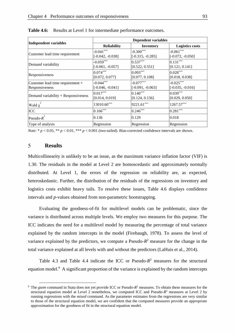
Chapter 4 Performance outcomes of responsiveness 93
Table 4.6: Results at Level 1 for intermediate performance outcomes.
Independent variables Dependent variables
Reliability Inventory Logistics costs
Customer lead time requirement -0.041***
[-0.042, -0.038]
-0.300***
[-0.315, -0.285]
-0.061***
[-0.072, -0.050]
Demand variability -0.059***
[-0.061, -0.057]
0.537***
[0.522, 0.551]
0.131***
[0.121, 0.141]
Responsiveness 0.074***
[0.072, 0.077]
0.093***
[0.077, 0.108]
0.028***
[0.018, 0.038]
Customer lead time requirement ×
Responsiveness
-0.044***
[-0.046, -0.041]
-0.077***
[-0.091, -0.063]
-0.025***
[-0.035, -0.016]
Demand variability × Responsiveness 0.017***
[0.014, 0.019]
0.140***
[0.124, 0.156]
0.039***
[0.029, 0.050]
Wald χ2 13010.60*** 9221.61*** 1267.57***
ICC 0.166*** 0.246*** 0.281***
Pseudo-R2 0.136 0.129 0.018
Type of analysis Regression Regression Regression
Note: * p < 0.05, ** p < 0.01, *** p < 0.001 (two-tailed). Bias-corrected confidence intervals are shown.
Results
Multicollinearity is unlikely to be an issue, as the maximum variance inflation factor (VIF) is
1.30. The residuals in the model at Level 2 are homoscedastic and approximately normally
distributed. At Level 1, the errors of the regression on reliability are, as expected,
heteroskedastic. Further, the distribution of the residuals of the regressions on inventory and
logistics costs exhibit heavy tails. To resolve these issues, Table 4.6 displays confidence
intervals and p-values obtained from non-parametric bootstrapping.
Evaluating the goodness-of-fit for multilevel models can be problematic, since the
variance is distributed across multiple levels. We employ two measures for this purpose. The
ICC indicates the need for a multilevel model by measuring the percentage of total variance
explained by the random intercepts in the model (Firebaugh, 1978). To assess the level of
variance explained by the predictors, we compute a Pseudo-R2 measure for the change in the
total variance explained at all levels with and without the predictors (LaHuis et al., 2014).
Table 4.3 and Table 4.4 indicate the ICC or Pseudo-R2 measures for the structural
equation model.9 A significant proportion of the variance is explained by the random intercepts
9 The gsem command in Stata does not yet provide ICC or Pseudo-R2 measures. To obtain these measures for the
structural equation model at Level 2 nonetheless, we computed ICC and Pseudo-R2 measures at Level 2 by
running regressions with the mixed command. As the parameter estimates from the regressions are very similar
to those of the structural equation model, we are confident that the computed measures provide an appropriate
approximation for the goodness of fit in the structural equation model.
Chapter 4 Performance outcomes of responsiveness 94
at Level 3 with an ICC of 0.337 for financial performance, 0.458 for reliability, 0.200 for
inventory and 0.598 for logistics costs. A statistically significant proportion of the variance is
explained for financial performance (Pseudo-R2 = 0.315 and Wald χ2 = 87.01, p < 0.001),
reliability (Pseudo-R2 = 0.178 and Wald χ2 = 34.53, p < 0.001) and inventory (Pseudo-R2 =
0.077 and Wald χ2 = 16.46, p < 0.01). However, the proportion of variance explained for
logistics costs is not statistically significant at the 5% level (Pseudo-R2 = 0.075 and Wald χ2 =
10.38, p = 0.07).
For the regressions at Level 1, Table 4.6 indicates that a significant proportion of the
variance is explained by the random intercepts at Level 2 and Level 3 for all three regression.
The ICC is 0.166 for reliability, 0.246 for inventory and 0.281 for logistics costs. The proportion
of variance explained is similar to the analysis at Level 2 for reliability (Pseudo-R2 = 0.136 and
Wald χ2 = 13010.60, p < 0.001), but higher for inventory (Pseudo-R2 = 0.129 and Wald χ2 =
9221.61, p < 0.001) and lower for logistics costs (Pseudo-R2 = 0.018 and Wald χ2 = 1267.57, p
< 0.001).
As endogeneity can lead to biased and inconsistent estimates, this study addresses three
main causes of endogeneity: measurement error, omitted variables and simultaneity (Roberts
and Whited, 2013). The control variables specified in Section 3.3 address concerns related to
omitted variables. Concerns regarding measurement error are addressed by minimizing the risk
of common method bias, as it is one of the main sources of measurement error (Podsakoff et
al., 2003). Common method bias is unlikely to be an issue for our study, as it relies exclusively
on archival data that is free from respondents’ perceptions and originates from multiple data
sources (financial and supply chain databases).
Concerns regarding simultaneity arise for the relationship between reliability and
financial performance. Hypothesis 2 suggests a positive relationship between these two
constructs, based on the argument that reliability increases financial performance by preventing
lost sales. However, one might also argue that the link between the two constructs is reverse:
business units with higher financial performance have more resources to invest in reliability.
For this reason, we conduct a Wu-Hausman specification test to assess whether reliability is an
exogenous estimator of financial performance (Hausman, 1978). Demand variability is used as
an instrumental variable for reliability for two reasons: (1) it is associated with lower reliability
as indicated by Table 4.5 and (2) it is not assumed to influence financial performance apart
from its negative effect on reliability. The residuals of the multilevel regression of demand
variability on reliability are not a statistically significant predictor of financial performance at
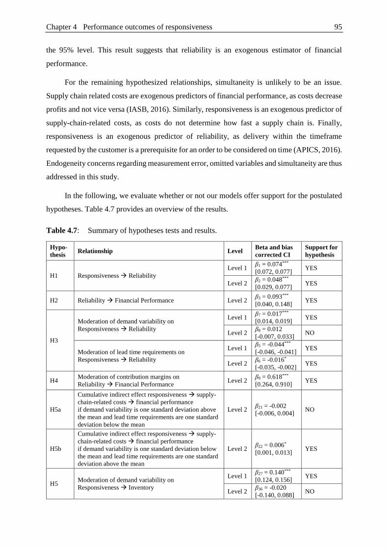
Chapter 4 Performance outcomes of responsiveness 95
the 95% level. This result suggests that reliability is an exogenous estimator of financial
performance.
For the remaining hypothesized relationships, simultaneity is unlikely to be an issue.
Supply chain related costs are exogenous predictors of financial performance, as costs decrease
profits and not vice versa (IASB, 2016). Similarly, responsiveness is an exogenous predictor of
supply-chain-related costs, as costs do not determine how fast a supply chain is. Finally,
responsiveness is an exogenous predictor of reliability, as delivery within the timeframe
requested by the customer is a prerequisite for an order to be considered on time (APICS, 2016).
Endogeneity concerns regarding measurement error, omitted variables and simultaneity are thus
addressed in this study.
In the following, we evaluate whether or not our models offer support for the postulated
hypotheses. Table 4.7 provides an overview of the results.
Table 4.7: Summary of hypotheses tests and results.
Hypo-
thesis Relationship Level
Beta and bias
corrected CI
Support for
hypothesis
H1 Responsiveness Reliability
Level 1 β1 = 0.074***
[0.072, 0.077] YES
Level 2 β2 = 0.048***
[0.029, 0.077] YES
H2 Reliability Financial Performance Level 2 β3 = 0.093***
[0.040, 0.148] YES
H3
Moderation of demand variability on
Responsiveness Reliability
Level 1 β7 = 0.017***
[0.014, 0.019] YES
Level 2 β8 = 0.012
[-0.007, 0.033] NO
Moderation of lead time requirements on
Responsiveness Reliability
Level 1 β5 = -0.044***
[-0.046, -0.041] YES
Level 2 β6 = -0.016*
[-0.035, -0.002] YES
H4 Moderation of contribution margins on
Reliability Financial Performance Level 2
β9 = 0.618***
[0.264, 0.910] YES
H5a
Cumulative indirect effect responsiveness supply-
chain-related costs financial performance
if demand variability is one standard deviation above
the mean and lead time requirements are one standard
deviation below the mean
Level 2 β21 = -0.002
[-0.006, 0.004] NO
H5b
Cumulative indirect effect responsiveness supply-
chain-related costs financial performance
if demand variability is one standard deviation below
the mean and lead time requirements are one standard
deviation above the mean
Level 2 β22 = 0.006*
[0.001, 0.013] YES
H5 Moderation of demand variability on
Responsiveness Inventory
Level 1 β27 = 0.140***
[0.124, 0.156] YES
Level 2 β36 = -0.020
[-0.140, 0.088] NO

Chapter 4 Performance outcomes of responsiveness 96
Moderation of lead time requirement on
Responsiveness Inventory
Level 1 β25 = -0.077***
[-0.091, -0.063] YES
Level 2 β20 = -0.139**
[-0.235, -0.050] YES
H5
Moderation of demand variability requirement on
Responsiveness Logistics Costs
Level 1 β28 = 0.039***
[0.029, 0.050] YES
Level 2 β37 = -0.105
[-0.221, 0.017] NO
Moderation of lead time requirement on
Responsiveness Logistics Costs
Level 1 β26 = -0.025***
[-0.035, -0.016] YES
Level 2 β38 = -0.061
[-0.154, 0.039] NO
H6
Inventory Financial Performance Level 2 β15 = -0.020**
[-0.030, -0.010] YES
Logistics Costs Financial Performance Level 2 β16 = -0.016***
[-0.024, -0.006] YES
Note: * p < 0.05, ** p < 0.01, *** p < 0.001 (two-tailed)
5.1 Responsiveness and the market mediation function
The proposed conceptual framework posits that responsiveness helps to match supply and
demand (Hypothesis 1) which prevents lost sales and therefore improves financial performance
(Hypothesis 2). Hypothesis 1 receives support at both Level 1 (β1 = 0.074, p < 0.001) and Level
2 (β2 = 0.048, p < 0.001). A one-standard-deviation change in responsiveness is associated with
a 7.4-percentage-point (ppt) increase in reliability at Level 1 and a 4.8ppt increase at Level 2.
Likewise, Hypothesis 2 is supported (β3 = 0.093, p < 0.01); a one-standard-deviation increase
in reliability (plus 14.4ppt) is associated with a 1.3ppt increase in the return on sales.
The theoretical model further states that these direct relationships are subject to several
moderating factors. Hypothesis 3 suggests that challenges in the operating environment (high
demand variability and short lead time requirements) increase the need for responsiveness and
thus positively moderate the relationship between responsiveness and reliability. As
hypothesized, the results indicate that the longer the customer lead time requirements (i.e.,
lower challenges), the weaker the relationship between responsiveness and reliability at Level
1 (β5 = -0.044, p < 0.001) and Level 2 (β6 = -0.016, p < 0.05). In the same vein, demand
variability positively moderates the relationship between responsiveness and reliability at Level
1 (β7 = 0.017, p < 0.001) and Level 2 (β8 = 0.012, p = 0.209). There is strong support for
Hypothesis 3, as three out of the four examined relationships are as hypothesized and
statistically significant. To better understand the statistically significant moderating effects of
lead time requirements and demand variability at both levels, Figure 4.5 shows the
corresponding interaction plots.
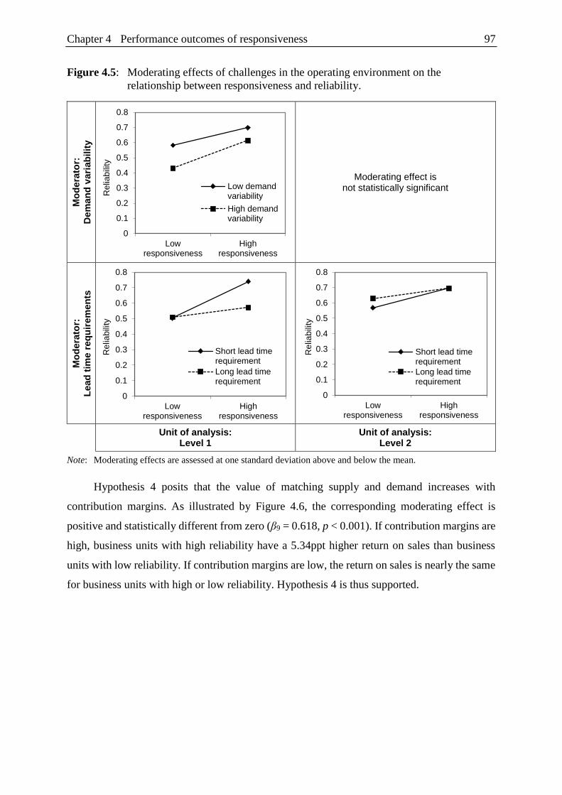
Chapter 4 Performance outcomes of responsiveness 97
Figure 4.5: Moderating effects of challenges in the operating environment on the
relationship between responsiveness and reliability. M
od
era
tor:
Dem
an
d v
ari
ab
ilit
y
Moderating effect is not statistically significant
Mo
dera
tor:
Lead
tim
e r
eq
uir
em
en
ts
Unit of analysis:
Level 1 Unit of analysis:
Level 2
Note: Moderating effects are assessed at one standard deviation above and below the mean.
Hypothesis 4 posits that the value of matching supply and demand increases with
contribution margins. As illustrated by Figure 4.6, the corresponding moderating effect is
positive and statistically different from zero (β9 = 0.618, p < 0.001). If contribution margins are
high, business units with high reliability have a 5.34ppt higher return on sales than business
units with low reliability. If contribution margins are low, the return on sales is nearly the same
for business units with high or low reliability. Hypothesis 4 is thus supported.
0
0.1
0.2
0.3
0.4
0.5
0.6
0.7
0.8
Lowresponsiveness
Highresponsiveness
Re
liab
ility
Low demandvariability
High demandvariability
0
0.1
0.2
0.3
0.4
0.5
0.6
0.7
0.8
Lowresponsiveness
Highresponsiveness
Relia
bili
ty
Short lead timerequirement
Long lead timerequirement
0
0.1
0.2
0.3
0.4
0.5
0.6
0.7
0.8
Lowresponsiveness
Highresponsiveness
Relia
bili
ty
Short lead timerequirement
Long lead timerequirement
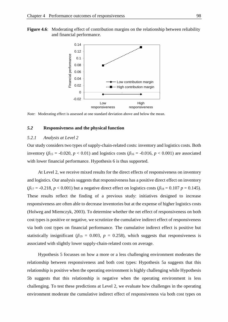
Chapter 4 Performance outcomes of responsiveness 98
Figure 4.6: Moderating effect of contribution margins on the relationship between reliability
and financial performance.
Note: Moderating effect is assessed at one standard deviation above and below the mean.
5.2 Responsiveness and the physical function
5.2.1 Analysis at Level 2
Our study considers two types of supply-chain-related costs: inventory and logistics costs. Both
inventory (β15 = -0.020, p < 0.01) and logistics costs (β16 = -0.016, p < 0.001) are associated
with lower financial performance. Hypothesis 6 is thus supported.
At Level 2, we receive mixed results for the direct effects of responsiveness on inventory
and logistics. Our analysis suggests that responsiveness has a positive direct effect on inventory
(β17 = -0.218, p < 0.001) but a negative direct effect on logistics costs (β18 = 0.107 p = 0.145).
These results reflect the finding of a previous study: initiatives designed to increase
responsiveness are often able to decrease inventories but at the expense of higher logistics costs
(Holweg and Miemczyk, 2003). To determine whether the net effect of responsiveness on both
cost types is positive or negative, we scrutinize the cumulative indirect effect of responsiveness
via both cost types on financial performance. The cumulative indirect effect is positive but
statistically insignificant (β19 = 0.003, p = 0.258), which suggests that responsiveness is
associated with slightly lower supply-chain-related costs on average.
Hypothesis 5 focusses on how a more or a less challenging environment moderates the
relationship between responsiveness and both cost types: Hypothesis 5a suggests that this
relationship is positive when the operating environment is highly challenging while Hypothesis
5b suggests that this relationship is negative when the operating environment is less
challenging. To test these predictions at Level 2, we evaluate how challenges in the operating
environment moderate the cumulative indirect effect of responsiveness via both cost types on
-0.02
0
0.02
0.04
0.06
0.08
0.1
0.12
0.14
Lowresponsiveness
Highresponsiveness
Fin
an
cia
l pe
rfo
rma
nce
Low contribution margin
High contribution margin

Chapter 4 Performance outcomes of responsiveness 99
financial performance. Out of the moderating effects examined here, only the effect of customer
lead time requirements on the relationship between responsiveness and inventory, shown in
Figure 4.7, is statistically significant (β20 = -0.140, p < 0.01). As a result, the cumulative indirect
effects of responsiveness via both cost types on financial performance is negative in a more
challenging operating environment (β21 = -0.002, p = 0.503) and positive in a less challenging
one (β22 = 0.006, p < 0.05). Responsiveness is thus associated with slightly higher costs in a
more challenging operating environment, but with lower costs in a less challenging operating
environment. Hypothesis 5 is therefore supported, but with two limitations.
Figure 4.7: Moderating effect of customer lead time requirements on the relationship between
responsiveness and inventory at Level 2.
Note: Moderating effect is assessed at one standard deviation above and below the mean.
First, there is only partial support for Hypothesis 5a, as the indirect effect between
responsiveness and financial performance is not statistically significant for a high level of
challenges in the operating environment. Business units with a more responsive supply chain
thus do not appear to incur significantly higher costs even if they operate in a challenging
environment. This is surprising, since levers for improving responsiveness that are used to deal
with challenges in the operating environment (e.g., airfreight or safety stock buffers) are
assumed to be costly.
Second, Hypothesis 5 claims that demand variability and customer lead time requirements
moderate the relationship between responsiveness and the two cost types. As we hypothesize
that there are two relevant moderators for each of the relationships between responsiveness and
the two cost types, there should be four statistically significant moderating effects. However,
only one out of the four hypothesized moderating effects is statistically significant.
-0.7
-0.5
-0.3
-0.1
0.1
0.3
Lowresponsiveness
Highresponsiveness
Inve
nto
ry
Short lead timerequirement
Long lead timerequirement
Chapter 4 Performance outcomes of responsiveness 100
To find out whether there are additional moderating effects at Level 1 that were not
discovered at Level 2, and to determine whether there are conditions given which higher
responsiveness is clearly associated with higher supply-chain-related costs, we examine
Hypothesis 5 at Level 1 as well.
5.2.2 Analysis at Level 1
There is a positive and statistically significant relationship between responsiveness and logistics
costs at Level 1 (β23 = 0.028, p < 0.001). Like the effect at Level 2, responsiveness is on average
associated with higher logistics costs at the product level.
For inventory, however, interpreting the direct effect is less straightforward. Although the
relationship between responsiveness and inventory is negative and statistically significant at
Level 2 (β17 = -0.218, p < 0.001), there is a positive and statistically significant relationship
between responsiveness and inventory at Level 1 (β24 = 0.093, p < 0.001). The difference
between the findings at Level 1 and Level 2 can be explained by the fact that practices designed
to reduce inventory by cutting lead times are typically adopted at the plant level (Shah and
Ward, 2003). The negative effect of responsiveness on inventory levels will therefore be hard
to observe at the product level, as products are often produced in several plants. Further, if
managers want to offer shorter lead times for a single product, it is more likely that they allocate
additional inventory to warehouses close to customers for that product than to initiate structural
changes in the supply chain. Consequently, it is not surprising that shorter lead times are on
average associated with higher inventories at a product level (e.g., due to build-up of safety
stock) and lower inventories at a business unit level (e.g., due to the effect of practices that aim
to reduce inventories at the business unit’s plants).
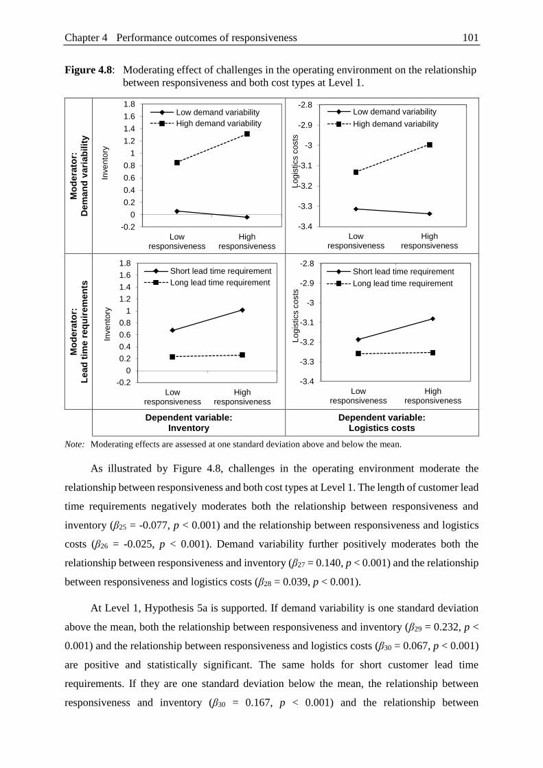
Chapter 4 Performance outcomes of responsiveness 101
Figure 4.8: Moderating effect of challenges in the operating environment on the relationship
between responsiveness and both cost types at Level 1. M
od
era
tor:
Dem
an
d v
ari
ab
ilit
y
Mo
dera
tor:
Lead
tim
e r
eq
uir
em
en
ts
Dependent variable:
Inventory Dependent variable:
Logistics costs
Note: Moderating effects are assessed at one standard deviation above and below the mean.
As illustrated by Figure 4.8, challenges in the operating environment moderate the
relationship between responsiveness and both cost types at Level 1. The length of customer lead
time requirements negatively moderates both the relationship between responsiveness and
inventory (β25 = -0.077, p < 0.001) and the relationship between responsiveness and logistics
costs (β26 = -0.025, p < 0.001). Demand variability further positively moderates both the
relationship between responsiveness and inventory (β27 = 0.140, p < 0.001) and the relationship
between responsiveness and logistics costs (β28 = 0.039, p < 0.001).
At Level 1, Hypothesis 5a is supported. If demand variability is one standard deviation
above the mean, both the relationship between responsiveness and inventory (β29 = 0.232, p <
0.001) and the relationship between responsiveness and logistics costs (β30 = 0.067, p < 0.001)
are positive and statistically significant. The same holds for short customer lead time
requirements. If they are one standard deviation below the mean, the relationship between
responsiveness and inventory (β30 = 0.167, p < 0.001) and the relationship between
-0.2
0
0.2
0.4
0.6
0.8
1
1.2
1.4
1.6
1.8
Lowresponsiveness
Highresponsiveness
Inve
nto
ryLow demand variability
High demand variability
-3.4
-3.3
-3.2
-3.1
-3
-2.9
-2.8
Lowresponsiveness
Highresponsiveness
Lo
gis
tics c
osts
Low demand variability
High demand variability
-0.2
0
0.2
0.4
0.6
0.8
1
1.2
1.4
1.6
1.8
Lowresponsiveness
Highresponsiveness
Inve
nto
ry
Short lead time requirement
Long lead time requirement
-3.4
-3.3
-3.2
-3.1
-3
-2.9
-2.8
Lowresponsiveness
Highresponsiveness
Lo
gis
tics c
osts
Short lead time requirement
Long lead time requirement
Chapter 4 Performance outcomes of responsiveness 102
responsiveness and logistics costs (β31 = 0.053, p < 0.001) are also positive and statistically
significant. Our results thus indicate that managers who aim to increase the responsiveness for
individual products are likely to incur higher supply-chain-related costs in a more challenging
operating environment.
Hypothesis 5b is only partially supported at Level 1. If demand variability is one standard
deviation below the mean, the relationship between responsiveness and inventory (β32 = -0.047,
p < 0.001) is negative and statistically significant. The relationship between responsiveness and
logistics costs is also negative but not statistically significant at the 95% level for low levels of
demand variability (β33 = -0.012, p = 0.07). If customer lead time requirements are below the
mean, both the relationship between responsiveness and inventory (β34 = 0.015, p = 0.06) and
the relationship between responsiveness and logistics costs (β35 = 0.003, p = 0.597) cease to be
statistically significant at the 95% level. While it thus might be difficult to achieve cost savings
by increasing the responsiveness of individual products in a less challenging operating
environment, there does not appear to be a trade-off between responsiveness and costs either.
In summary, our results support Hypothesis 5. Both demand variability and customer lead
time requirements are important moderators of the relationship between responsiveness and the
examined cost types. Hypothesis 5a is supported, as responsiveness is associated with
significantly higher supply-chain-related costs at Level 1 and slightly higher supply-chain-
related costs at Level 2 in a more challenging operating environment. Further, there is support
for Hypothesis 5b at Level 2, as business units’ responsiveness is associated with lower supply-
chain-related costs in a less challenging operating environment. At Level 1, there is partial
support for Hypothesis 5b, as there does not appear to be a trade-off between responsiveness
and costs for individual products in a less challenging operating environment. Our results thus
indicate that responsiveness entails a cost premium in a more challenging operating
environment and is associated with cost reductions in a less challenging operating environment.
Discussion and implications
A popular framework for assessing the value of responsiveness has been proposed by Fisher
(1997): the importance of matching supply and demand is higher for innovative products –
accordingly responsiveness is more important for innovative products as well.
Our results, however, indicate that responsiveness is important for both functional and
innovative products. On the one hand, challenges in the operating environment positively
moderate the relationship between responsiveness and reliability; contribution margins further
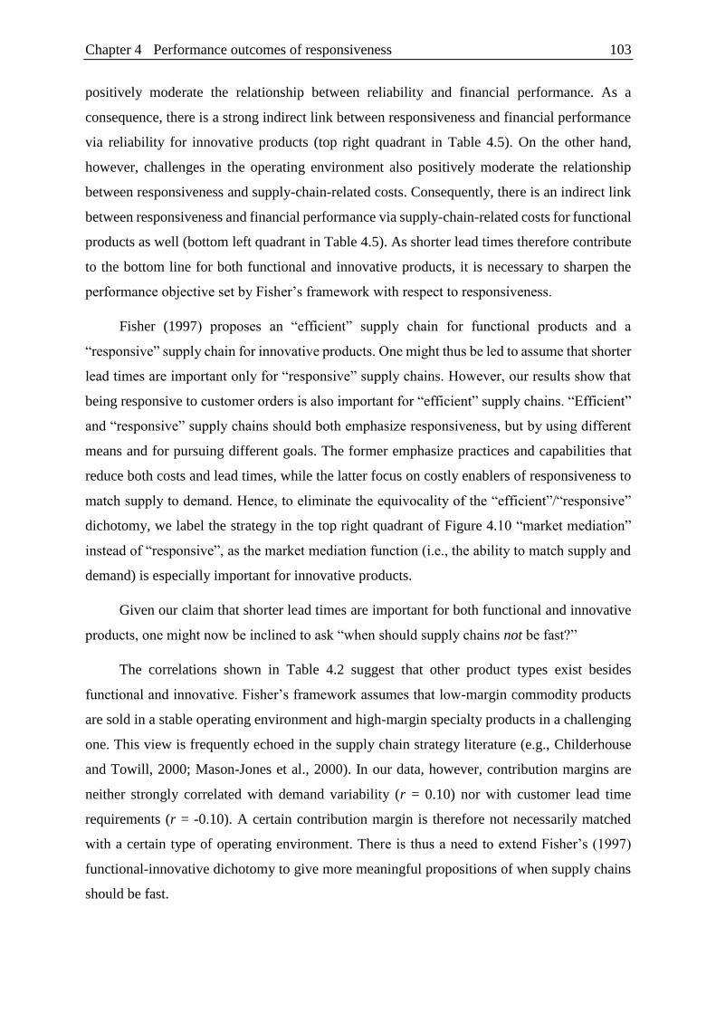
Chapter 4 Performance outcomes of responsiveness 103
positively moderate the relationship between reliability and financial performance. As a
consequence, there is a strong indirect link between responsiveness and financial performance
via reliability for innovative products (top right quadrant in Table 4.5). On the other hand,
however, challenges in the operating environment also positively moderate the relationship
between responsiveness and supply-chain-related costs. Consequently, there is an indirect link
between responsiveness and financial performance via supply-chain-related costs for functional
products as well (bottom left quadrant in Table 4.5). As shorter lead times therefore contribute
to the bottom line for both functional and innovative products, it is necessary to sharpen the
performance objective set by Fisher’s framework with respect to responsiveness.
Fisher (1997) proposes an “efficient” supply chain for functional products and a
“responsive” supply chain for innovative products. One might thus be led to assume that shorter
lead times are important only for “responsive” supply chains. However, our results show that
being responsive to customer orders is also important for “efficient” supply chains. “Efficient”
and “responsive” supply chains should both emphasize responsiveness, but by using different
means and for pursuing different goals. The former emphasize practices and capabilities that
reduce both costs and lead times, while the latter focus on costly enablers of responsiveness to
match supply to demand. Hence, to eliminate the equivocality of the “efficient”/“responsive”
dichotomy, we label the strategy in the top right quadrant of Figure 4.10 “market mediation”
instead of “responsive”, as the market mediation function (i.e., the ability to match supply and
demand) is especially important for innovative products.
Given our claim that shorter lead times are important for both functional and innovative
products, one might now be inclined to ask “when should supply chains not be fast?”
The correlations shown in Table 4.2 suggest that other product types exist besides
functional and innovative. Fisher’s framework assumes that low-margin commodity products
are sold in a stable operating environment and high-margin specialty products in a challenging
one. This view is frequently echoed in the supply chain strategy literature (e.g., Childerhouse
and Towill, 2000; Mason-Jones et al., 2000). In our data, however, contribution margins are
neither strongly correlated with demand variability (r = 0.10) nor with customer lead time
requirements (r = -0.10). A certain contribution margin is therefore not necessarily matched
with a certain type of operating environment. There is thus a need to extend Fisher’s (1997)
functional-innovative dichotomy to give more meaningful propositions of when supply chains
should be fast.
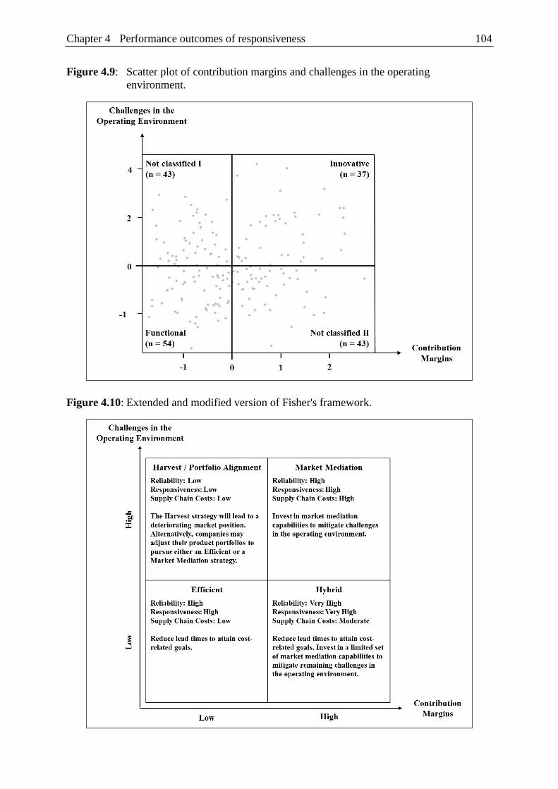
Chapter 4 Performance outcomes of responsiveness 104
Figure 4.9: Scatter plot of contribution margins and challenges in the operating
environment.
Figure 4.10: Extended and modified version of Fisher's framework.
Chapter 4 Performance outcomes of responsiveness 105
Figure 4.9 illustrates that the distribution of business units in our sample according to
contribution margins and challenges in the operating environment. As with the left-hand side
of Table 4.5, challenges in the operating environment are measured by the standardized
logarithm of demand variability minus the standardized logarithm of customer lead time
requirements.10 Although there is a positive correlation between contribution margins and
challenges in the operating environment (r = 0.14), there are many business units that cannot
be classified as manufacturers of functional or innovative products. Business units in the
bottom-left quadrant (n = 54) can be classified as manufacturers of functional products and
business units in the top-right quadrant (n = 37) as manufacturers of innovative products.
However, for manufacturers of low-margin products with high challenges in the operating
environment (n = 43), no classification is provided by Fisher’s framework. The same is true for
business units in the bottom-right quadrant (n = 43) that manufacture high margins products in
a less challenging operating environment.
To clarify the role of the responsiveness for these unclassified business units, we extend
Fisher’s framework by the two additional supply chain strategies shown in Figure 4.10. Based
on our findings, the strategies not only indicate whether supply chains should be fast, but also
specify targets for the match been supply and demand (reliability) and supply-chain-related
costs. The four strategies are detailed next.
The “market mediation” strategy in the top-right quadrant applies to companies selling
high-margin products in a challenging operating environment (e.g., fashion retailers). They
should aim for a high level of reliability, since high contribution margins increase the adverse
effect of lost sales on profitability. Given the high level of demand variability and/or short
customer lead time requirements, they need to invest in matching supply and demand. Our
findings indicate that improving responsiveness is effective for this task. Other capabilities for
matching supply and demand such as agility or flexibility could also fit well with this strategy
(Anand and Ward, 2004; Gligor et al., 2015; Gligor, 2015; Merschmann and Thonemann, 2011;
Qi et al., 2009; Qi et al., 2011; Wagner et al., 2012). However, we focus our recommendations
for this strategy on reliability, responsiveness and cost-related targets, since agility and
flexibility were not examined as part of our study. Accordingly, we advise managers pursuing
a market mediation strategy to set ambitious targets for reliability and responsiveness, but also
to accept higher supply chain costs.
10 We take the logarithm of both variables, as we assume diminishing effects. The two variables are standardized
to make their scales comparable.
Chapter 4 Performance outcomes of responsiveness 106
The “efficient” strategy in the bottom-left quadrant applies to manufacturers of low-
margin products operating in an environment with few challenges (e.g., producers of canned
soup). Since demand is stable and customer grant sufficient time to react to uncertainties,
reliability should be high even without investments in capabilities that match supply and
demand. Low contribution margins also leave little room for such investments. Thus, managers
should aim for a high level of reliability at relatively low cost. Our findings highlight that shorter
lead times are a key enabler of this strategy, because they help to both reduce supply-chain-
related costs and increase reliability in an operating environment with few challenges.
Consequently, we advise managers pursuing a physically efficient supply chain to aim for high
levels of reliability and responsiveness while keeping supply-chain-related costs relatively low.
The “hybrid” strategy in the bottom-right quadrant is applicable to companies that offer
high-margin products in an operating environment with few challenges (e.g., producers of
patent-protected pharmaceuticals). It is a hybrid of the “market mediation” and the “efficient”
strategy. High contribution margins incentivize managers to aim for high reliability. However,
since demand is relatively stable and/or customer grant sufficient time to react to uncertainties,
there is only a limited need to invest in capabilities that match supply and demand. Similar to
the “efficient” strategy, shorter lead times enable the attainment of cost-related goals, as the
level of challenges in the operating environment is low. In addition, managers may invest in a
limited set of capabilities for matching supply and demand if there are remaining challenges in
their operating environment that need to be mitigated. Managers pursuing this strategy are
advised to aim for very high levels of reliability and responsiveness (via practices that improve
both efficiency and responsiveness and – if necessary – costly enablers of lead time reductions)
at moderate supply chain costs.
The “harvest” and the “portfolio alignment” strategies in the top-left quadrant apply to
companies that offer low-margin products in an operating environment characterized by time
pressure and demand volatility. They are caught in an unfortunate situation, since challenges in
the operating environment create a need for investing in capabilities such as responsiveness to
match supply and demand. However, investments of this type would not pay off because of low
contribution margins. As reflected by the results in the top-left quadrant of Table 4.5, the value
of responsiveness is thus low for companies operating in such an environment. To deal with
this issue, managers can either implement a low-cost supply chain that fails to reliably meet
customer demand. This would be equivalent of adopting a “harvest” strategy for “dogs” of the
BCG Matrix, where costs are reduced at the expense of a deteriorating market position

Chapter 4 Performance outcomes of responsiveness 107
(Barksdale and Harris, 1982). Alternatively, managers may adjust their product portfolio. So
far we have matched supply chain strategies to the requirements of the operating environment
although decisions regarding the product portfolio and supply chain strategy are interdependent
(Seifert and Langenberg, 2011; Seifert et al., 2016). Managers can remove products with low
margins or sporadic demand from their portfolio (Godsell et al., 2011). Removing the former
from the product portfolio would render the pursuit of a market mediation strategy attractive,
while removing the latter would enable the setting up of a physically efficient supply chain.
Limitations and future research directions
When interpreting the findings of this research, one must be aware of its methodological
limitations. First, our data was gathered for a single period which limits the extent to which
cause-and-effect relationships can be inferred. Second, we examined data only from a single
company (BASF). Although the company is diverse in terms of the operational and competitive
environments its business units face, the relationships among the examined variables might be
different for other companies and other industries. The moderating effect of contribution
margins, for example, might be less pronounced for tier-one suppliers in the automotive
industry, as they require nearly perfect reliability regardless of their contribution margins due
to the high penalty costs charged by OEMs for late deliveries (Guiffrida and Nagi, 2006). Third,
this study has relied exclusively on secondary data from BASF databases. An advantage of
secondary data is its objectivity, as there is no risk of diluted respondent perception (Calantone
and Vickery, 2009). However, although we trust the data used for this study, the risk of a
systematic measurement error by the company’s databases cannot be ruled out completely;
replication and validation studies are therefore needed. Finally, our strict reliance on secondary
data has limited the scope of our study and therefore presents opportunities for future research.
In particular, future studies may evaluate additional intermediate performance outcomes
of supply chain responsiveness. This study assessed the implications of responsiveness for
inventory and logistics costs. However, shorter lead times are also associated with costs of, for
instance, procurement or manufacturing (de Treville et al., 2014b; Mackelprang and Nair,
2010). The remaining positive (but not statistically significant) direct effect of responsiveness
on financial performance indicates that other cost types might be affected by shorter lead times.
Benefits of responsiveness not considered in this study such as a shorter time-to-market are also
a potential cause of the remaining direct effect. Assessing additional benefits and costs

Chapter 4 Performance outcomes of responsiveness 108
associated with shorter lead times would thus provide a fuller picture of the performance
outcomes of responsiveness.

Chapter 5 Summary, limitations and outlook 109
Chapter 5 Summary, limitations and outlook
This chapter summarizes the main results of this thesis with regards to the research questions
formulated in Chapter 1. Further, it highlights the limitations of our studies and outlines
potentials for future research.
Summary of the research questions
Aligning the competitive priorities of supply chains with the requirements of the business
environment is critical for competing successfully in the marketplace. Nonetheless,
misalignment is frequent in practice, as key challenges companies face when seeking alignment
remain unresolved. The introductory chapter identified three of these challenges and formulated
corresponding research questions. The studies in Chapter 2, 3 and 4 intended to answer these
questions; the results are summarized in the following.
1.1 Research Question 1: Capturing requirements of the business environment
Companies are confronted with a wide variety of potentially relevant contingency variables,
but with little guidance as to which of these variables they should take into consideration when
developing supply chain strategies. Consequently, Research Question 1 was concerned with
disambiguating which contingencies are important for setting the competitive priorities of
supply chains. The research question was:
Question 1: Which contingency variables should companies analyse in order to
capture supply-chain-relevant requirements of their business?
Answering this question required a two-step approach. First, given the wide variety of
contingencies, there was a need to clarify why the contingencies proposed in the extant
literature are potentially relevant for achieving alignment. For this purpose, we categorized
proposed contingencies based on how they affect the relative importance of competitive
priorities. Second, to determine which of these contingencies should be considered for deriving
strategies, we tested whether their proposed effects on the relative importance of competitive
priorities are large enough to be taken into consideration when developing strategies.
Hence, at first, Chapter 2 developed a typology in order to clarify why different types of
contingencies are potentially relevant for developing supply chain strategies. It highlights that
contingencies may affect the relative importance of competitive priorities in two distinct ways.
Chapter 5 Summary, limitations and outlook 110
On the one hand, challenges in the operating environment make it harder to fulfil demand
as requested by customers, ceteris paribus. As a result, contingency variables of this type
indicate to what extent companies require market mediation capabilities to avoid lost sales.
Challenges in the operating environment can be further subclassified into demand-related (e.g.,
demand variability), time-related (e.g., customer lead time requirements) and supply-related
(e.g., time-specificity of input-materials). On the other hand, contingencies affecting the value
of market mediation indicate to what extent a failure to fulfil demand as requested by customers
adversely affects a company’s bottom line. Consequently, contingencies of this type determine
whether the benefits of investing in market mediation capabilities in a challenging operating
environment outweigh the associated costs.
For a subset of the categorized contingencies, Chapter 2 then tested whether the effects
put forward by the typology are large enough for these variables to be taken into consideration
when developing strategies. Specifically, the chapter analysed to what extent five challenges in
the operating environment that are referred to as DWV3 affect the ability to fulfil demand as
requested by customers. The chapter restricted its analysis to the DWV3 variables (product
lifecycle Duration, customer lead time requirements / delivery time Window, demand
Variability, demand Volume, product Variety), since they are the most frequently cited
variables in the literature on supply chain strategy (Christopher et al., 2009). We hypothesized
that these variables affect the ability to reliably fulfil demand as requested in different ways:
whereas demand variability and customer lead time requirements were expected to affect
reliability directly, we hypothesized that the remaining DWV3 variables would affect reliability
indirectly by increasing demand variability.
The analysis was conducted at two levels: the hypotheses were tested with a multilevel
structural equation models at the business-unit-level and with multilevel regressions at the
product-level. As expected, the findings linked high demand variability and short lead time
requirements directly and consistently to lower reliability. For the remaining variables, the link
to reliability was mostly indirect: apart from being associated with higher demand variability,
these variables only marginally affected the ability of supply chains to fulfil demand as
requested by customers. Consequently, we concluded that demand variability and customer lead
time requirements need to be taken into consideration when developing supply chain strategies,
as they indicate to what extent companies require market mediation capabilities to reliably fulfil
demand. Volume, variety and lifecycle duration are less important for this purpose, but may
instead be used for analysing the causes of variable demand.
Chapter 5 Summary, limitations and outlook 111
Finally, in addition to the challenges in the operating environment analysed in Chapter 2,
Chapter 4 examined whether contribution margins need to be taken into consideration when
developing supply chain strategies. As part of an analysis on the performance outcomes of
responsiveness, the chapter tested whether contribution margins increase the positive effect of
reliability on financial performance. The results indicated a significant and positive moderating
effect, hence demonstrating that contribution margins are a key determinant of the value of
market mediation.
1.2 Research Question 2: Data-driven supply chain segmentation
Supply chain segmentation describes the process of dividing a heterogeneous set of products,
customers or business units into groups (“segments”) that impose similar requirements on the
supply chain. Because such a segmentation allows companies to tailor their supply chains more
closely to the requirements of their business, the topic currently receives significant attention
from practitioners (Gartner, 2016a). Despite this attention, extant studies on supply chain
segmentation almost exclusively form segments qualitatively, even though this approach is
considered “probably the […] least effective” (Wedel, 2000). Given the resultant need for
alternative approaches to forming supply chain segments, Research Questions 2a and 2b were
formulated as follows:
Question 2a: How can companies use data-driven methods to form supply chain
segments quantitatively?
Question 2b: What insights do these data-driven methods generate relative to
qualitative approaches?
As a first step towards answering this question, Chapter 3 highlighted the shortcomings
of approaches to forming supply chain segments proposed by extant studies on the topic.
Qualitative approaches – which are prevalent in the literature – are subjective and, hence, may
cause relevant clusters of products or customers to remain undetected. The quantitative
approach introduced by Langenberg et al. (2012) requires companies to specify potential supply
chain design options with quantifiable performance implications before the segmentation. As a
result, it provides guidance at the tactical rather than the strategic level of decision making.
Given these shortcomings, the research in Chapter 3 then proceeded to demonstrate how
companies can conduct a supply chain segmentation using two data-driven methods that are
popular in other areas of business research: clustering and classification.
Chapter 5 Summary, limitations and outlook 112
First, we conducted a cluster analysis to form an initial set of segments. For this purpose,
the clustering algorithm Mclust was used for grouping together business units that were similar
with respect to demand variability, customer lead time requirements and contribution margins.
We employed the Mclust algorithm, since the examined business units did not exhibit a clear
cluster structure and the algorithm allows for overlapping clusters. The cluster analysis was
conducted with data on business units from the years 2013 and 2014 to enable a comparison
with a set of supply chain segments BASF had formed qualitatively during the same time period
and using the same level of aggregation. The analysed contingency variables were chosen based
on the results of this thesis for Research Question 1.
The cluster analysis identified a set of four actionable, stable and externally valid supply
chain segments. In accordance to strategies that match the characteristics of these segments,
they were labelled “Lean” (low variability and low margins), “Agile” (high variability, high
margins and long lead time requirements), “Leagile” (high variability, high margins and short
lead time requirements), and “Basic Service” (high variability and low margins). The
characteristics of the first three segments corresponded to BASF’s qualitative segments, hence
allowing for a comparison between quantitative and the qualitative segments. For this purpose,
we examined the link between mismatches (i.e., business units that had assigned themselves to
a segment different from the one proposed by the cluster analysis) and financial performance.
The results linked mismatches to significantly lower financial performance. The findings
therefore implied that clustering is a feasible approach for developing supply chain segments
and for detecting cases where managers have selected segments that do not adequately reflect
the requirements of their business.
Finally, Chapter 3 examined how classification can be used to update and review existing
segments. For this purpose, the segments established by the cluster analysis for data from the
years 2013 and 2014 was used to train a random forest algorithm. The algorithm then classified
data on BASF business units from the years 2015. 21% of business units were assigned to a
different segment by the algorithm, in most cases because of a change in the level of
contribution margins or demand variability. We therefore concluded that classification
algorithms are important for sustaining a portfolio of supply chain segments, since the contexts
in which supply chains operate change over time.
Chapter 5 Summary, limitations and outlook 113
1.3 Research Question 3: Performance outcomes of responsiveness
In supply chain management, responsiveness describes the ability of a supply chain to fulfil
orders within a time frame that is acceptable to the customer. Even though setting lead-time-
related targets is considered critical for achieving aligned alignment, there are conflicting
perspectives as to when short lead times should be prioritized. Consequently, Research
Question 3 was concerned with the performance outcomes of responsiveness. The research
question was:
Question 3: When should companies make supply chain responsiveness a competitive
priority?
The conflicting perspectives regarding the performance outcomes of responsiveness
emanate from two – largely disconnected – literature streams. On the one hand, studies on the
value of shorter lead times argue that responsiveness entails a cost premium and, hence, purport
that responsiveness is primarily important for innovative products (e.g., de Treville et al.,
2014a). On the other hand, studies on lean management and just-in-time practices assert that
shorter lead times reduce supply-chain-related costs (e.g., Shah and Ward, 2003). To clarify in
which contexts shorter lead times positively contribute to a company’s bottom line, the research
in Chapter 4 examined both the benefits and the costs of responsiveness.
Regarding the benefits of responsiveness, we hypothesized that shorter lead times enable
companies to fulfil demand as requested by customers and, hence, positively impacts the bottom
line by preventing lost sales. Further, we hypothesized that the benefits are higher in contexts
that are characteristic of innovative products – i.e., challenging operating environments with
high margins – for two reasons. First, we suspected more opportunities for reducing lost sales
by decreasing lead times in environments characterized by volatile demand and time pressure.
Second, we expected high contribution margins to increase the positive effect of avoiding lost
sales on the bottom line.
Regarding the costs of responsiveness, we hypothesized that companies can leverage lean
management and just-in-time practices to achieve both lead time and cost savings in contexts
that are characteristic of functional products, i.e., where demand is stable and lead time
requirements are long. For challenging operating environments, we hypothesized that
responsiveness entails a cost premium.
Similar to the research in Chapter 2, we conducted our analyses at two levels: the
hypotheses were tested with a multilevel structural equation models at the business-unit-level
Chapter 5 Summary, limitations and outlook 114
and with multilevel regressions at the product-level. As expected, the findings indicated that
responsiveness can increase financial performance for both innovative and functional products.
In challenging operating environments with high contribution margins, shorter lead times
increase financial performance by matching supply and demand, hence preventing the loss of
high-margin sales. In environments characterized by stable demand and long lead time
requirements, shorter lead times contribute to the bottom line by reducing supply-chain-related
costs.
Further, as our sample comprised business units that could be classified neither as
manufacturers of innovative products nor as manufacturers of functional products, we extended
our propositions to two additional contexts. For high-margin businesses facing little time
pressure and stable demand, we proposed leveraging responsiveness to reduce costs and for
mitigating remaining challenges in the operating environment. For low-margin businesses
facing a challenging operating environment, we proposed that managers refrain from
prioritizing responsiveness, as the resulting increase in low-margin sales might fail to offset the
associated increase in costs.
Limitations
When interpreting the findings of this thesis, one must be aware of its methodological
limitations.
First, our research analysed cross-sectional data which limits the extent to which cause-
and-effect relationships can be inferred. All relationships tested in the studies of this thesis were
scrutinized for simultaneity. For one relationship where simultaneity was considered plausible
– the relationship between reliability and financial performance in Chapter 4 – the results of a
Wu-Hausman specification test suggested that the analysed predictor is exogenous.
Nonetheless, the threats of simultaneity and reverse causality cannot be ruled out entirely.
Second, this thesis has analysed data from a single company (BASF). Although BASF is
diverse in terms of the operational and competitive environments its business units face, the
relationships among the examined variables might be different for other companies and other
industries. The link between mismatches and financial performance, for instance, might be
different for companies operating in a different industry, as the relationship between fit and
performance is subject to a number of industry-level moderators (Gligor, 2017). Similarly,
companies using clustering to form supply chain segments quantitatively may arrive at a
different set of segments, as characteristics of product and business unit portfolios differ
Chapter 5 Summary, limitations and outlook 115
between firms (Protopappa-Sieke and Thonemann, 2017). Hence, even though the BASF data
used in this thesis constitutes a sufficiently broad and heterogeneous empirical basis to warrant
the generalization of our findings, replication and validation studies are needed.
Third, given our reliance on archival company data, the studies in this thesis were at risk
of omitting variables that (1) affect the examined relationships, but (2) are not available in
company databases. The research in Chapter 2, for instance, did not account for the competitive
priorities of the business units in our sample, even though they might have systematically
affected the (absolute) effect sizes of the examined relationships. Similarly, when assessing the
mismatch-performance link in Chapter 3, we would have liked to control for the resources the
examined business units had available for preventing mismatches, since they might have
affected both mismatches and performance. While our studies were able to draw inferences
nonetheless – Chapter 2 examined relative effect sizes and Chapter 3 used business unit size as
a proxy for resource availability – additional qualitative information would have rendered our
findings more robust.
Fourth, the regressions in Chapter 2 and 4 employed maximum likelihood estimators even
though one of the dependent variables (reliability) was bounded between zero and one. Since
maximum likelihood estimators assume a continuous distribution of the dependent variable, the
regression results were heteroskedastic. Zero-or-one inflated beta regressions – a potential
remedy when response variables follow a mixed continuous–discrete distribution with
probability mass at zero or one – are not yet available for multilevel models. To be able to draw
inferences nonetheless, we obtained heteroscedasticity-robust standard errors from non-
parametric bootstrapping. However, once methods for conducting zero-or-one inflated beta
regressions with multilevel data are available, validation studies are needed to review the
robustness of our results.
Finally, in addition to the outlined methodological limitations, the thesis at hand is subject
to conceptual limitations that are addressed in the following section.
Outlook
The introductory chapter identified three key challenges that prevent companies from attaining
supply chain fit. While the studies in this thesis have contributed towards filling these gaps,
opportunities for future research remain.

Chapter 5 Summary, limitations and outlook 116
Contingency variables affect the relative importance of competitive priorities in different
ways. This thesis has investigated the effects hypothesized to be underlying variables of three
types: demand-related challenges in the operating environment, time-related challenges in the
operating environment and contingencies affecting the value of market mediation. However,
the effects underlying supply-related challenges in the operating environment have not been
empirically examined so far. Contingencies of this type are increasingly receiving attention in
the extant literature (Ho et al., 2015), yet it is not sufficiently clear which variables need to be
considered when developing supply chain strategies. Ho et al. (2005), for instance, propose that
companies should analyse a set of seven reflective measures of manufacturing-related and
supplier-related uncertainties for this purpose. However, most of the proposed measurement
items are not available in company databases and so far there has been no empirical examination
to what extent these measures affect the ability to fulfil demand as requested by customers.
Further research is also needed on data-driven approaches for supply chain segmentation.
On the one hand, replication and validation studies may scrutinize the benefits of clustering and
classification outlined by this research. As the characteristics of product and customer portfolios
vary between companies, it would be worthwhile to enquire whether other firms would also be
able to find an actionable set of segments with the proposed methods. On the other hand, there
are opportunities for advancing the research presented in Chapter 3. Possible extensions include
the use of a wider range of clustering and classification methods, cluster analysing products or
customers instead of business units, or the development of approaches that explicitly combine
qualitative and quantitative information from the beginning. Given the attention the topic
currently receives from practitioners and the benefits of conducting a data-driven segmentation
outlined by this thesis, we are confident that further research on this issue will emerge.
Finally, out of the examined research questions, arguably the largest potential for future
studies lies in enabling managers to derive strategies that align with the (segment-specific)
requirements of their business. This thesis has investigated the context-dependency of benefits
and costs associated with responsiveness. Future research may extend this analysis by
considering additional contingencies, benefits or costs. However, disambiguating the
performance outcomes of responsiveness constitutes only a first step towards enabling
companies to achieve alignment. In particular, further work is needed to (1) delineate which
capabilities are important for achieving alignment, (2) how these capabilities should be
operationalized and (3) what their antecedents and consequences are.
Chapter 5 Summary, limitations and outlook 117
Consider, for instance, the case of supply chain agility, a market mediation capability that
is considered critical for competing successfully in a turbulent business environment (Lee,
2004). A recent literature review identified 26 different definitions of supply chain agility that
exhibit considerable overlap to closely related constructs such as flexibility (Sharma et al.,
2017). The review also identified a lack of consensus as to what relevant antecedents of supply
chain agility are. Further, there are inconsistent propositions regarding the performance
outcomes of supply chain agility. Even though most studies find that supply chain agility is a
market mediation capability that entails a cost premium (Agarwal et al., 2006; Goldsby et al.,
2006; Narasimhan et al., 2006), an empirical study by Gligor et al. (2015) suggests that agility
can improve both efficiency and customer effectiveness. Hence, in spite of being considered
critical for achieving alignment, it is not sufficiently clear what supply chain agility is, how it
can be achieved and when it should be pursued.
The fact that recent literature reviews have made similar findings for other market
mediation capabilities such as flexibility and resilience (Tukamuhabwa et al., 2015; Yu et al.,
2015) highlights that there is significant ambiguity as to which capabilities are important for
achieving alignment. As stated in Chapter 2, proposed market mediation capabilities range from
different aspects of responsiveness (e.g., Bernardes and Hanna, 2009), agility (e.g., Gligor et
al., 2013), flexibility (e.g., Swafford et al., 2006) to different sources of resilience (e.g., Pettit
et al., 2010). Consequently, further research is needed to delineate which capabilities are
relevant for aligning supply chain strategies and how these capabilities should be
operationalized.
Once a set of well-defined market mediation capabilities has been specified, future studies
may investigate its antecedents and consequences. Comprehending the consequences of market
mediation capabilities is critical for determining when they should be prioritized; investigating
their antecedents is imperative for enabling companies to put their strategies into practice. It is
only if the antecedents and consequences of a well-defined set of market mediation capabilities
are unambiguous that this area of research will be able to adequately support companies in
developing aligned supply chain strategies.

Chapter 5 Summary, limitations and outlook 118
References 119
References
Agarwal, A., Shankar, R., Tiwari, M.K., 2006. Modeling the metrics of lean, agile and leagile
supply chain: An ANP-based approach. European Journal of Operational Research 173 (1),
211–225.
Aggarwal, C.C., 2015. Data Classification: Algorithms and Applications. CRC Press, Boca
Ranton, USA.
Aitken, J., Childerhouse, P., Christopher, M., Towill, D., 2005. Designing and managing
multiple pipelines. Journal of Business Logistics 26 (2), 73–96.
American Chemical Society, 2017. Global Top 50 Chemical Companies 2017. Chemical &
Engineering News. https://cen.acs.org/articles/95/i30/CENs-Global-Top-
50.html?type=paidArticleContent. Accessed 16 October 2017.
Amtsgericht Bonn, 2017. Insolvenzbekanntmachung SolarWorld AG.
https://www.insolvenzbekanntmachungen.de/cgi-
bin/bl_aufruf.pl?PHPSESSID=689b9651f8be4f20186102d010c5de53&datei=gerichte/nw/
agbonn/17/0099_IN00079_17/2017_08_01__11_21_30_Eroeffnung_Insolvenzverfahren.h
tm. Accessed 5 September 2017.
Amtsgericht München, 2009. Insolvenzbekanntmachung Qimonda AG.
https://www.insolvenzbekanntmachungen.de/cgi-
bin/bl_aufruf.pl?PHPSESSID=aa19c6b8c8cb84a773bacc6a91c1cbeb&datei=gerichte/by/a
gmuenchen/09/1542_IN_209_09/2009_08_06__15_20_02_Termine.htm. Accessed 5
September 2017.
Anand, G., Ward, P.T., 2004. Fit, flexibility and performance in manufacturing: coping with
dynamic environments. Production and Operations Management 13 (4), 369–385.
APICS, 2016. Supply Chain Operations Reference Model: SCOR Model - Version 11.
Accessed 18 October 2016.
Azadegan, A., Patel, P.C., Zangoueinezhad, A., Linderman, K., 2013. The effect of
environmental complexity and environmental dynamism on lean practices. Journal of
Operations Management 31 (4), 193–212.
Bacher, J., Pöge, A., Wenzig, K., 2010. Clusteranalyse: Anwendungsorientierte Einführung in
Klassifikationsverfahren. Oldenbourg Verlag, Munich, Germany.
Barksdale, H.C., Harris, C.E., 1982. Portfolio analysis and the product life cycle. Long Range
Planning 15 (6), 74–83.
BASF SE, 2015. BASF Annual Report 2014. http://bericht.basf.com/2014/en/. Accessed 10
March 2016.
BASF SE, 2016a. BASF Annual Report 2015. http://bericht.basf.com/2015/en/. Accessed 18
October 2016.
BASF SE, 2016b. Verbund. https://www.basf.com/en/company/about-us/strategy-and-
organization/verbund.html. Accessed 1 February 2017.
BASF SE, 2017. Segments. https://www.basf.com/en/company/investor-relations/basf-at-a-
glance/business-segments.html. Accessed 21 April 2017.
Basnet, C., Seuring, S., 2016. Demand-Oriented Supply Chain Strategies - A Review of
Literature. Operations and Supply Chain Management 9 (2), 73–89.
Baum, C.F., 2008. Stata tip 63: Modeling proportions. Stata Journal 8 (2), 299.
Bernardes, E., Hanna, M.D., 2009. A theoretical review of flexibility, agility and
responsiveness in the operations management literature: Toward a conceptual definition of
customer responsiveness. International Journal of Operations & Production Management 29
(1), 30–53.
Blackburn, J., 2012. Valuing time in supply chains: establishing limits of time-based
competition. Journal of Operations Management 30 (5), 396–405.

References 120
Bozarth, C.C., Warsing, D.P., Flynn, B.B., Flynn, E.J., 2009. The impact of supply chain
complexity on manufacturing plant performance. Journal of Operations Management 27 (1),
78–93.
Breiman, L., 2001. Random forests. Machine learning 45 (1), 5–32.
Brock, G., Pihur, V., Datta, S., Datta, S., 2011. clValid: An R package for cluster validation.
Journal of Statistical Software 25 (4), 1–22.
Browning, T.R., Heath, R.D., 2009. Reconceptualizing the effects of lean on production costs
with evidence from the F-22 program. Journal of Operations Management 27 (1), 23–44.
Brusco, M., Singh, R., Cradit, J.D., Steinley, D., 2017. Cluster analysis in empirical OM
research: survey and recommendations. International Journal of Operations & Production
Management 37 (3), 300–320.
Brusco, M., Steinley, D., Cradit, J.D., Singh, R., 2012. Emergent clustering methods for
empirical OM research. Journal of Operations Management 30 (6), 454–466.
Burbidge, J.B., Magee, L., Robb, A.L., 1988. Alternative transformations to handle extreme
values of the dependent variable. Journal of the American Statistical Association 83 (401),
123–127.
Calantone, R., Vickery, S.K., 2009. Special topic forum on using archival and secondary data
sources in supply chain management research. Journal of Supply Chain Management 45 (2),
94–95.
Cambridge Dictionary, 2016. Meaning of “responsiveness” in the English Dictionary.
http://dictionary.cambridge.org/dictionary/english/responsiveness. Accessed 28 August
2016.
Cariou, P., 2011. Is slow steaming a sustainable means of reducing CO2 emissions from
container shipping? Transportation Research Part D: Transport and Environment 16 (3),
260–264.
Cecere, L., 2017. BASF: A Story of a Supply Chain Leader.
http://www.supplychainshaman.com/supply-chain-2/supply-chain-excellence/basf-a-story-
of-a-supply-chain-leader/. Accessed 13 April 2017.
Chavez, R., Yu, W., Jacobs, M., Fynes, B., Wiengarten, F., Lecuna, A., 2015. Internal lean
practices and performance: The role of technological turbulence. International Journal of
Production Economics 160, 157–171.
Chen, I.J., Paulraj, A., Lado, A.A., 2004. Strategic purchasing, supply management, and firm
performance. Journal of Operations Management 22 (5), 505–523.
Childerhouse, P., Aitken, J., Towill, D., 2002. Analysis and design of focused demand chains.
Journal of Operations Management 20 (6), 675–689.
Childerhouse, P., Towill, D., 2000. Engineering supply chains to match customer requirements.
Logistics Information Management 13 (6), 337–346.
Chopra, S., Sodhi, M.S., 2014. Reducing the risk of supply chain disruptions. MIT Sloan
Management Review 55 (3), 73–80.
Christopher, M., Gattorna, J., 2005. Supply chain cost management and value-based pricing.
Industrial Marketing Management 34 (2), 115–121.
Christopher, M., Lowson, R., Peck, H., 2004. Creating agile supply chains in the fashion
industry. International Journal of Retail & Distribution Management 32 (8), 367–376.
Christopher, M., Peck, H., Towill, D., 2006. A taxonomy for selecting global supply chain
strategies. The International Journal of Logistics Management 17 (2), 277–287.
Christopher, M., Towill, D., 2002. Developing market specific supply chain strategies. The
International Journal of Logistics Management 13 (1), 1–14.
Christopher, M., Towill, D., Aitken, J., Childerhouse, P., 2009. Value stream classification.
Journal of Manufacturing Technology Management 20 (4), 460–474.
Clarke, B., Fokoue, E., Zhang, H.H., 2009. Principles and theory for data mining and machine
learning. Springer, New York, USA.

References 121
CNN, 2016. Gap still getting clobbered by 'fast fashion'.
http://money.cnn.com/2016/05/09/news/companies/gap-sales-decline/index.html.
Accessed 4 September 2017.
Cooil, B., Keiningham, T.L., Aksoy, L., Hsu, M., 2007. A longitudinal analysis of customer
satisfaction and share of wallet: Investigating the moderating effect of customer
characteristics. Journal of Marketing 71 (1), 67–83.
Cook, D.O., Kieschnick, R., McCullough, B.D., 2008. Regression analysis of proportions in
finance with self selection. Journal of Empirical Finance 15 (5), 860–867.
Craighead, C.W., Blackhurst, J., Rungtusanatham, M.J., Handfield, R.B., 2007. The severity of
supply chain disruptions: design characteristics and mitigation capabilities. Decision
Sciences 38 (1), 131–156.
Croom, S., Christensen, W.J., Germain, R., Birou, L., 2007. Variance vs average: supply chain
lead-time as a predictor of financial performance. Supply Chain Management: An
International Journal 12 (5), 349–357.
Damanpour, F., 1992. Organizational size and innovation. Organization studies 13 (3), 375–
402.
de Leeuw, S., van den Berg, J., 2011. Improving operational performance by influencing
shopfloor behavior via performance management practices. Journal of Operations
Management 29 (3), 224–235.
de Paepe, P., McLinn, J., Porter, M., 2015. Responding to oil price volatility in the chemical
industry. http://www.bain.com/publications/articles/responding-to-oil-price-volatility-in-
the-chemical-industry.aspx. Accessed 5 April 2017.
de Treville, S., Biçer, I., Chavez-Demoulin, V., Hagspiel, V., Schürhoff, N., Tasserit, C.,
Wager, S., 2014a. Valuing lead time. Journal of Operations Management 32 (6), 337–346.
de Treville, S., Schürhoff, N., Trigeorgis, L., Avanzi, B., 2014b. Optimal Sourcing and Lead‐
Time Reduction under Evolutionary Demand Risk. Production and Operations Management
23 (12), 2103–2117.
de Treville, S., Shapiro, R.D., Hameri, A.-P., 2004. From supply chain to demand chain: the
role of lead time reduction in improving demand chain performance. Journal of Operations
Management 21 (6), 613–627.
Dibb, S., Simkin, L., 2009. Implementation rules to bridge the theory/practice divide in market
segmentation. Journal of Marketing Management 25 (3-4), 375–396.
Dolnicar, S., Grün, B., 2008. Challenging “factor–cluster segmentation”. Journal of Travel
Research 47 (1), 63–71.
Donaldson, L., 2001. The contingency theory of organizations. Sage, Thousand Oaks, CA.
Droge, C., Jayaram, J., Vickery, S.K., 2004. The effects of internal versus external integration
practices on time-based performance and overall firm performance. Journal of Operations
Management 22 (6), 557–573.
Duda, R.O., Hart, P.E., Stork, D.G., 2012. Pattern classification. John Wiley & Sons, New
York, USA.
Elgazzar, S.H., Tipi, N.S., Hubbard, N.J., Leach, D.Z., 2012. Linking supply chain processes’
performance to a company’s financial strategic objectives. European Journal of Operational
Research 223 (1), 276–289.
Everitt, B., Landau, S., Leese, M., Stahl, D., 2011. Cluster Analysis. Wiley, Chichester, UK.
Ferdows, K., Lewis, M.A., Machuca, J.A.D., 2004. Rapid-fire fulfillment. Harvard Business
Review 82 (11), 104–110.
Ferrari, S., Cribari-Neto, F., 2004. Beta regression for modelling rates and proportions. Journal
of Applied Statistics 31 (7), 799–815.
Firebaugh, G., 1978. A rule for inferring individual-level relationships from aggregate data.
American sociological review 43 (4), 557–572.

References 122
Fisher, M.L., 1997. "What is the right supply chain for your product?". Harvard Business
Review 75 (2), 105–117.
Foedermayr, E.K., Diamantopoulos, A., 2008. Market segmentation in practice: Review of
empirical studies, methodological assessment, and agenda for future research. Journal of
Strategic Marketing 16 (3), 223–265.
Forbes, 2015. Gap Inc Is Gradually Losing Its Share In The U.S. Apparel Market To Fast-
Fashion Counterparts. https://www.forbes.com/sites/greatspeculations/2015/07/15/gap-inc-
is-gradually-losing-its-share-in-the-u-s-apparel-market-to-fast-fashion-
counterparts/#72735552b0e1. Accessed 5 September 2017.
Fraley, C., Raftery, A.E., 2002. Model-based Clustering, Discriminant Analysis and Density
Estimation. Journal of the American Statistical Association 97 (458), 611–663.
Fuller, J., O'Conor, J., Rawlinson, R., 1993. Tailored logistics: the next advantage. Harvard
Business Review 71 (3), 87–98.
Gartner, I., 2016a. For Supply Chain Executives: How Segmentation Supports New Growth
and Efficiencies. https://www.gartner.com/doc/3270717/supply-chain-executives-
segmentation-supports. Accessed 5 October 2016.
Gartner, I., 2016b. The Hierarchy of Supply Chain Metrics: Diagnosing Your Supply Chain
Health. https://www.gartner.com/doc/3083323/hierarchy-supply-chain-metrics-
diagnosing. Accessed 10 July 2016.
Gligor, D., Esmark, C.L., Holcomb, M.C., 2015. Performance outcomes of supply chain agility:
when should you be agile? Journal of Operations Management 33 (1), 71–82.
Gligor, D., Holcomb, M.C., Stank, T.P., 2013. A multidisciplinary approach to supply chain
agility: Conceptualization and scale development. Journal of Business Logistics 34 (2), 94–
108.
Gligor, D., 2015. The Role of Supply Chain Agility in Achieving Supply Chain Fit. Decision
Sciences 47 (3), 524–553.
Gligor, D., 2017. Re‐Examining Supply Chain Fit: An Assessment of Moderating Factors.
Journal of Business Logistics.
Godfrey, L., 2009. Bootstrap Methods for Regression Models with Non-IID Errors, in: Godfrey,
L. (Ed.), Bootstrap Tests for Regression Models. Springer, Cham, Switzerland, pp. 177–
217.
Godsell, J., Diefenbach, T., Clemmow, C., Towill, D., Christopher, M., 2011. Enabling supply
chain segmentation through demand profiling. International Journal of Physical Distribution
& Logistics Management 41 (3), 296–314.
Godsell, J., Harrison, A., Emberson, C., Storey, J., 2006. Customer responsive supply chain
strategy: An unnatural act? International Journal of Logistics 9 (1), 47–56.
Goldsby, T.J., Griffis, S.E., Roath, A.S., 2006. Modeling lean, agile, and leagile supply chain
strategies. Journal of Business Logistics 27 (1), 57–80.
Goldsby, T.J., Martichenko, R., 2005. Lean six sigma logistics: Strategic development to
operational success. J. Ross, Plantation, USA.
Grosse-Ruyken, P.T., Wagner, S.M., 2010. Does supply chain “Fit” matter to investors. Supply
Chain Quarterly 4 (4), 44–50.
Guiffrida, A.L., Nagi, R., 2006. Cost characterizations of supply chain delivery performance.
International Journal of Production Economics 102 (1), 22–36.
Habermann, M., Blackhurst, J., Metcalf, A.Y., 2015. Keep your friends close? Supply chain
design and disruption risk. Decision Sciences 46 (3), 491–526.
Hausman, J.A., 1978. Specification tests in econometrics. Econometrica 46 (6), 1251–1271.
Hendricks, K.B., Singhal, V.R., 2003. The effect of supply chain glitches on shareholder
wealth. Journal of Operations Management 21 (5), 501–522.
Hendricks, K.B., Singhal, V.R., 2005. Association between supply chain glitches and operating
performance. Management Science 51 (5), 695–711.

References 123
Ho, C.-F., Tai, Y.-M., Chi, Y.-P., 2005. A structural approach to measuring uncertainty in
supply chains. International Journal of Electronic Commerce 9 (3), 91–114.
Ho, W., Zheng, T., Yildiz, H., Talluri, S., 2015. Supply chain risk management: a literature
review. International Journal of Production Research 53 (16), 5031–5069.
Hofmann, D.A., 1997. An overview of the logic and rationale of hierarchical linear models.
Journal of Management 23 (6), 723–744.
Holweg, M., Miemczyk, J., 2003. Delivering the ‘3-day car’—the strategic implications for
automotive logistics operations. Journal of Purchasing and Supply Management 9 (2), 63–
71.
Holweg, M., 2005. The three dimensions of responsiveness. International Journal of Operations
& Production Management 25 (7), 603–622.
Hong, S., Musso, C., Simons, T.J., 2015. Oil-price shocks and the chemical industry: Preparing
for a volatile environment. http://www.mckinsey.com/industries/chemicals/our-
insights/oil-price-shocks-and-the-chemical-industry-preparing-for-a-volatile-environment.
Accessed 5 April 2017.
IASB, 2016. IAS Standard 1: Presentation of Financial Statements.
http://www.ifrs.org/IFRSs/Pages/IFRS.aspx. Accessed 22 November 2016.
Infineon Technologies AG, 2006. Annual Report.
https://www.infineon.com/dgdl/2006_IFX_20-
F.pdf?fileId=db3a3043324cae8c01326323efe339cc. Accessed 5 September 2017.
Jian, M., Fang, X., Jin, L.-q., Rajapov, A., 2015. The impact of lead time compression on
demand forecasting risk and production cost: A newsvendor model. Transportation
Research Part E: Logistics and Transportation Review 84, 61–72.
Ketchen, D.J., Shook, C.L., 1996. The application of cluster analysis in strategic management
research: an analysis and critique. Strategic Management Journal 17 (6), 441–458.
Ketokivi, M., McIntosh, C.N., 2017. Addressing the endogeneity dilemma in operations
management research: Theoretical, empirical, and pragmatic considerations. Journal of
Operations Management 52, 1–14.
Kinkel, S., Maloca, S., 2009. Drivers and antecedents of manufacturing offshoring and
backshoring - A German perspective. Journal of Purchasing and Supply Management 15
(3), 154–165.
Kotsiantis, S.B., 2007. Supervised Machine Learning: A Review of Classification Techniques,
in: Proceedings of the 2007 conference on Emerging Artificial Intelligence Applications in
Computer Engineering: Real Word AI Systems with Applications in eHealth, HCI,
Information Retrieval and Pervasive Technologies. IOS Press, Amsterdam, The
Netherlands, pp. 3–24.
LaHuis, D.M., Hartman, M.J., Hakoyama, S., Clark, P.C., 2014. Explained variance measures
for multilevel models. Organizational Research Methods 17 (4), 433–451.
Langenberg, K.U., Seifert, R.W., Tancrez, J.-S., 2012. Aligning supply chain portfolios with
product portfolios. International Journal of Production Economics 135 (1), 500–513.
Lee, H.L., 2002. Aligning Supply Chain Strategies with Product Uncertainties. California
Management Review 44 (3), 105–119.
Lee, H.L., 2004. The triple-A supply chain. Harvard Business Review 82 (10), 102–113.
Liaw, A., Wiener, M., 2002. Classification and regression by randomforest. R News 2 (3), 18–
22.
Lovell, A., Saw, R., Stimson, J., 2005. Product value-density: managing diversity through
supply chain segmentation. The International Journal of Logistics Management 16 (1), 142–
158.
Mackelprang, A.W., Nair, A., 2010. Relationship between just-in-time manufacturing practices
and performance: A meta-analytic investigation. Journal of Operations Management 28 (4),
283–302.

References 124
Mansfield, E., 1993. The diffusion of flexible manufacturing systems in Japan, Europe and the
United States. Management Science 39 (2), 149–159.
Mason-Jones, R., Naylor, B., Towill, D., 2000. Lean, agile or leagile? Matching your supply
chain to the marketplace. International Journal of Production Research 38 (17), 4061–4070.
Mayer, S., Thiry, E., Frank, C.B., 2009. 6th European AT Kearney/ELA Logistics Study
2008/2009: Supply Chain Excellence Amidst the Global Economic Crisis.
Merschmann, U., Thonemann, U.W., 2011. Supply chain flexibility, uncertainty and firm
performance: An empirical analysis of German manufacturing firms. International Journal
of Production Economics 130 (1), 43–53.
Milligan, G.W., 1996. Clustering validation: results and implications for applied analyses, in:
Arabie, P., Hubert, L.J., de Soete, G. (Eds.), Clustering and classification. World Scientific,
Singapore, pp. 341–375.
Narasimhan, R., Swink, M., Kim, S.W., 2006. Disentangling leanness and agility: an empirical
investigation. Journal of Operations Management 24 (5), 440–457.
Naylor, B., Naim, M.M., Berry, D., 1999. Leagility: integrating the lean and agile
manufacturing paradigms in the total supply chain. International Journal of Production
Economics 62 (1), 107–118.
Ngai, E.W.T., Xiu, L., Chau, D.C.K., 2009. Application of data mining techniques in customer
relationship management: A literature review and classification. Expert Systems with
Applications 36 (2), 2592–2602.
Olhager, J., 2003. Strategic positioning of the order penetration point. International Journal of
Production Economics 85 (3), 319–329.
Ospina, R., Ferrari, S., 2012. A general class of zero-or-one inflated beta regression models.
Computational Statistics & Data Analysis 56 (6), 1609–1623.
Papke, L., Woolridge, J., 1996. Econometric methods for fractional response variables with an
application to 401 (k) plan participation rates. Journal of Applied Econometrics 11, 619–
632.
Payne, T., Peters, M.J., 2004. What is the right supply chain for your products? The
International Journal of Logistics Management 15 (2), 77–92.
Peng, Y., Dong, M., Zuo, M.J., 2010. Current status of machine prognostics in condition-based
maintenance: a review. The International Journal of Advanced Manufacturing Technology
50 (1), 297–313.
Perera, C., Zaslavsky, A., Christen, P., Georgakopoulos, D., 2014. Context aware computing
for the internet of things: A survey. IEEE Communications Surveys & Tutorials 16 (1), 414–
454.
Pettit, T.J., Fiksel, J., Croxton, K.L., 2010. Ensuring supply chain resilience: development of a
conceptual framework. Journal of Business Logistics 31 (1), 1–21.
Podsakoff, P.M., MacKenzie, S.B., Lee, J.-Y., Podsakoff, N.P., 2003. Common method biases
in behavioral research: a critical review of the literature and recommended remedies. Journal
of Applied Psychology 88 (5), 879–903.
Preacher, K.J., Zyphur, M.J., Zhang, Z., 2010. A general multilevel SEM framework for
assessing multilevel mediation. Psychological Methods 15 (3), 209.
Protopappa-Sieke, M., Thonemann, U.W., 2017. Supply Chain Segmentation: Best-in-Class
Cases, Practical Insights and Foundations. Springer, Cham, Switzerland.
Qi, Y., Boyer, K.K., Zhao, X., 2009. Supply chain strategy, product characteristics, and
performance impact: Evidence from Chinese manufacturers. Decision Sciences 40 (4), 667–
695.
Qi, Y., Zhao, X., Sheu, C., 2011. The Impact of Competitive Strategy and Supply Chain
Strategy on Business Performance: The Role of Environmental Uncertainty. Decision
Sciences 42 (2), 371–389.
References 125
Randall, T., Morgan, R.M., Morton, A.R., 2003. Efficient versus Responsive Supply Chain
Choice: An Empirical Examination of Influential Factors. Journal of Product Innovation
Management 20 (6), 430–443.
Randall, T., Ulrich, K., 2001. Product Variety, Supply Chain Structure, and Firm Performance:
Analysis of the US Bicycle Industry. Management Science 47 (12), 1588–1604.
Reuters, 2017a. Emerging markets, online growth help Zara-owner Inditex outpace H&M.
http://www.reuters.com/article/us-inditex-results/emerging-markets-online-growth-help-
zara-owner-inditex-outpace-hm-idUSKBN16M0YP. Accessed 5 September 2017.
Reuters, 2017b. SolarWorld collapses as Europe's solar industry eclipsed by China.
http://www.reuters.com/article/us-sma-solar-results/solarworld-collapses-as-europes-solar-
industry-eclipsed-by-china-idUSKBN1870ZV. Accessed 5 September 2017.
Rexhausen, D., Pibernik, R., Kaiser, G., 2012. Customer-facing supply chain practices - The
impact of demand and distribution management on supply chain success. Journal of
Operations Management 30 (4), 269–281.
Roberts, M.R., Whited, T.M., 2013. Endogeneity in Empirical Corporate Finance, in:
Constantinides, G.M., Harris, M., Stulz, R.M. (Eds.), Handbook of the Economics of
Finance, Volume 2, Part A. Elsevier, Amsterdam, Netherlands, pp. 493–572.
Roscoe, S., Baker, P., 2014. Supply chain segmentation in the sporting goods industry.
International Journal of Logistics Research and Applications 17 (2), 136–155.
Seifert, R.W., Langenberg, K.U., 2011. Managing business dynamics with adaptive supply
chain portfolios. European Journal of Operational Research 215 (3), 551–562.
Seifert, R.W., Tancrez, J.-S., Biçer, I., 2016. Dynamic product portfolio management with life
cycle considerations. International Journal of Production Economics 171, 71–83.
Selig, J.P., Preacher, K.J., 2008. Monte Carlo method for assessing mediation: An interactive
tool for creating confidence intervals for indirect effects [Computer software].
http://quantpsy.org/. Accessed 26 May 2017.
Selldin, E., Olhager, J., 2007. Linking products with supply chains: testing Fisher's model.
Supply Chain Management: An International Journal 12 (1), 42–51.
Shah, R., Ward, P.T., 2003. Lean manufacturing: context, practice bundles, and performance.
Journal of Operations Management 21 (2), 129–149.
Sharma, N., Sahay, B.S., Shankar, R., Sarma, P.R., 2017. Supply chain agility: review,
classification and synthesis. International Journal of Logistics Research and Applications
20 (6), 532–559.
Shepherd, C., Günter, H., 2006. Measuring supply chain performance: current research and
future directions. International Journal of Productivity and Performance Management 55
(3/4), 242–258.
Simangunsong, E., Hendry, L.C., Stevenson, M., 2012. Supply-chain uncertainty: a review and
theoretical foundation for future research. International Journal of Production Research 50
(16), 4493–4523.
Snijders, T.A.B., 2011. Multilevel analysis. Springer, Heidelberg, Germany.
Solarworld Industries AG, 2009. U.S. headquarters and largest solar module production facility
in the Americas. https://www.solarworld-usa.com/about-solarworld/locations. Accessed 5
September 2017.
Sousa, R., Voss, C.A., 2008. Contingency research in operations management practices. Journal
of Operations Management 26 (6), 697–713.
Steele, F., Goldstein, H., 2006. Multilevel models in psychometrics, in: C.R. Rao, S. Sinharay
(Eds.), Psychometrics, vol. 26. Elsevier, Amsterdam, Netherlands, pp. 401–420.
Sugimori, Y., Kusunoki, K., Cho, F., Uchikawa, S., 1977. Toyota production system and
kanban system materialization of just-in-time and respect-for-human system. The
International Journal of Production Research 15 (6), 553–564.
References 126
Swafford, P., Ghosh, S., Murthy, N., 2006. The antecedents of supply chain agility of a firm:
Scale development and model testing. Journal of Operations Management 24 (2), 170–188.
The Economist, 2009. The semiconductor industry - Under new management.
http://www.economist.com/node/13405279. Accessed 5 September 2017.
The Economist, 2015. Faster, cheaper fashion.
https://www.economist.com/news/business/21663221-rapidly-rising-super-cheap-irish-
clothes-retailer-prepares-conquer-america-rivals-should. Accessed 4 September 2017.
Tukamuhabwa, B.R., Stevenson, M., Busby, J., Zorzini, M., 2015. Supply chain resilience:
definition, review and theoretical foundations for further study. International Journal of
Production Research 53 (18), 5592–5623.
Tuli, P., Shankar, R., 2015. Collaborative and lean new product development approach: a case
study in the automotive product design. International Journal of Production Research 53 (8),
2457–2471.
van de Ven, A., Ganco, M., Hinings, C., 2013. Returning to the frontier of contingency theory
of organizational and institutional designs. Academy of Management Annals 7 (1), 393–
440.
van der Leeden, R., Meijer, E., Busing, F., 2008. Resampling multilevel models, in: de Leeuw,
J., Meijer, E. (Eds.), Handbook of Multilevel Analysis. Springer, New York City, USA,
pp. 401–433.
Venkatraman, N., 1989. The concept of fit in strategy research: Toward verbal and statistical
correspondence. Academy of management Review 14 (3), 423–444.
Verhoef, P.C., Spring, P.N., Hoekstra, J.C., Leeflang, P.S.H., 2003. The commercial use of
segmentation and predictive modeling techniques for database marketing in the
Netherlands. Decision Support Systems 34 (4), 471–481.
Verma, M., Verter, V., 2010. A lead-time based approach for planning rail–truck intermodal
transportation of dangerous goods. European Journal of Operational Research 202 (3), 696–
706.
Vijayasarathy, L.R., 2010. Supply integration: An investigation of its multi-dimensionality and
relational antecedents. International Journal of Production Economics 124 (2), 489–505.
Wagner, S.M., Grosse-Ruyken, P.T., Erhun, F., 2012. The link between supply chain fit and
financial performance of the firm. Journal of Operations Management 30 (4), 340–353.
Wangenheim, F., Bayon, T., 2004. Satisfaction, loyalty and word of mouth within the customer
base of a utility provider: Differences between stayers, switchers and referral switchers.
Journal of Consumer Behaviour 3 (3), 211–220.
Wedel, M., 2000. Market segmentation: Conceptual and methodological foundations. Springer,
New York, USA.
Yu, K., Cadeaux, J., Luo, B.N., 2015. Operational flexibility: Review and meta-analysis.
International Journal of Production Economics 169, 190–202.
Zotteri, G., Kalchschmidt, M., 2007. A model for selecting the appropriate level of aggregation
in forecasting processes. International Journal of Production Economics 108 (1), 74–83.

Curriculum Vitae 127
Curriculum Vitae
Christian Joachim Freiherr von Falkenhausen accomplished his secondary education at the
Brentwood College School in Mill Bay, British Columbia, Canada in 2008. Subsequently, he
studied business and economics at the University of Exeter, UK. After receiving his Bachelor’s
degree in 2011, he enrolled at the University of Mannheim, Germany, to purse a Master’s
degree in business studies. Following his graduation in 2014, he commenced his doctoral
studies at the Chair of Logistics and Supply Chain Management of the University of Mannheim
where he was employed as a research assistant.