Three-dimensional virtual refocusing of fluorescence microscopy images using

deep learning

Authors:

Yichen Wu1,2,3,†, Yair Rivenson1,2,3,†, Hongda Wang1,2,3, Yilin Luo1,2,3, Eyal Ben-David4, Laurent

A. Bentolila3,5, Christian Pritz6, Aydogan Ozcan1,2,3,7,*

1 Electrical and Computer Engineering Department, University of California, Los Angeles,

California 90095, USA

2 Bioengineering Department, University of California, Los Angeles, California 90095, USA

3 California Nano Systems Institute (CNSI), University of California, Los Angeles, California

90095, USA

4 Department of Human Genetics, David Geffen School of Medicine, University of California,

Los Angeles, California 90095, USA

5 Department of Chemistry and Biochemistry, University of California, Los Angeles, CA, 90095,

USA

6 Department of Genetics, Hebrew University of Jerusalem, Edmond J. Safra Campus, Givat

Ram, Jerusalem, 91904, Israel

7 Department of Surgery, David Geffen School of Medicine, University of California, Los

Angeles, California 90095, USA

†Equal contribution authors

*Corresponding author, email: ozcan@ucla.edu

Abstract:

Three-dimensional (3D) fluorescence microscopy in general requires axial scanning to capture

images of a sample at different planes. Here we demonstrate that a deep convolutional neural

network can be trained to virtually refocus a 2D fluorescence image onto user-defined 3D

surfaces within the sample volume. With this data-driven computational microscopy framework,

we imaged the neuron activity of a Caenorhabditis elegans worm in 3D using a time-sequence of

fluorescence images acquired at a single focal plane, digitally increasing the depth-of-field of the

microscope by 20-fold without any axial scanning, additional hardware, or a trade-off of imaging

resolution or speed. Furthermore, we demonstrate that this learning-based approach can correct

for sample drift, tilt, and other image aberrations, all digitally performed after the acquisition of a

single fluorescence image. This unique framework also cross-connects different imaging

modalities to each other, enabling 3D refocusing of a single wide-field fluorescence image to

match confocal microscopy images acquired at different sample planes. This deep learning-based

3D image refocusing method might be transformative for imaging and tracking of 3D biological

samples, especially over extended periods of time, mitigating photo-toxicity, sample drift,

aberration and defocusing related challenges associated with standard 3D fluorescence

microscopy techniques.

Text:

Three-dimensional (3D) fluorescence microscopic imaging is essential for biomedical and

physical sciences as well as engineering, covering various applications 1–7. Despite its broad

importance, high-throughput acquisition of fluorescence image data for a 3D sample remains a

challenge in microscopy research. 3D fluorescence information is usually acquired through

scanning across the sample volume, where several 2D fluorescence images/measurements are

obtained, one for each focal plane or point in 3D , which forms the basis of e.g., confocal 8, two-

photon 5, light-sheet 7,9,10 or various super-resolution 2,4,11–14 microscopy techniques. However,

because scanning is used, the image acquisition speed and the throughput of the system for

volumetric samples are limited to a fraction of the frame-rate of the camera/detector, even with

optimized scanning strategies 8 or point-spread function (PSF) engineering 7,15. Moreover,

because the images at different sample planes/points are not acquired simultaneously, the

temporal variations of the sample fluorescence can inevitably cause image artifacts. Another

concern is the photo-toxicity of illumination and photo-bleaching of fluorescence since parts of

the sample can be repeatedly excited during the scanning process.

To overcome some of these challenges, non-scanning 3D fluorescence microscopy methods have

also been developed, so that the entire 3D volume of the sample can be imaged at the same speed

as the detector framerate. One of these methods is fluorescence light-field microscopy 6,16–19.

This system typically uses an additional micro-lens array to encode the 2D angular information

as well as the 2D spatial information of the sample light rays into image sensor pixels; then a 3D

focal stack can be digitally reconstructed from this recorded 4D light-field. However, using a

micro-lens array reduces the spatial sampling rate which results in a sacrifice of both the lateral

and axial resolution of the microscope. Although the image resolution can be improved by 3D

deconvolution 6 or compressive sensing 17 techniques, the success of these methods depends on

various assumptions regarding the sample and the forward model of the image formation

process. Furthermore, these computational approaches are relatively time-consuming as they

involve an iterative hyperparameter tuning as part of the image reconstruction process. A related

method termed multi-focal microscopy has also been developed to map the depth information of

the sample onto different parallel locations within a single image 20,21. However, the improved

3D imaging speed of this method also comes at the cost of reduced imaging resolution or field-

of-view (FOV) and can only infer an experimentally pre-defined (fixed) set of focal planes

within the sample volume. As another alternative, the fluorescence signal can also be optically

correlated to form a Fresnel correlation hologram, encoding the 3D sample information in

interference patterns 22–24. To retrieve the missing phase information, this computational

approach requires multiple images to be captured for volumetric imaging of a sample. Quite

importantly, all these methods summarized above, and many others, require the addition of

customized optical components and hardware into a standard fluorescence microscope,

potentially needing extensive alignment and calibration procedures, which not only increase the

cost and complexity of the optical set-up, but also cause potential aberrations and reduced

photon-efficiency for the fluorescence signal.

Here we introduce a digital image refocusing framework in fluorescence microscopy by training

a deep neural network using microscopic image data, enabling 3D imaging of fluorescent

samples using a single 2D wide-field image, without the need for any mechanical scanning,

additional hardware or parameter estimation. This data-driven fluorescence image refocusing

framework does not need a physical model of the imaging system, and rapidly refocuses a 2D

fluorescence image onto user-defined 3D surfaces. In addition to rapid 3D imaging of a

fluorescent sample volume, it can also be used to digitally correct for various aberrations due to

the sample and/or the optical system. We term this deep learning-based approach Deep-Z, and

use it to computationally refocus a single 2D wide-field fluorescence image onto 3D surfaces

within the sample volume, without sacrificing the imaging speed, spatial resolution, field-of-

view, or throughput of a standard fluorescence microscope.

In Deep-Z framework, an input 2D fluorescence image (to be digitally refocused onto a 3D

surface within the sample volume) is first appended with a user-defined digital propagation

matrix (DPM) that represents, pixel-by-pixel, the axial distance of the target surface from the

plane of the input image (Fig. 1). Deep-Z is trained using a conditional generative adversarial

neural network (GAN) 25,26 using accurately matched pairs of (1) various fluorescence images

axially-focused at different depths and appended with different DPMs, and (2) the corresponding

fluorescence images (i.e., the ground truth labels) captured at the correct/target focus plane

defined by the corresponding DPM. Through this training process that only uses experimental

image data without any assumptions or physical models, the generator network of GAN learns to

interpret the values of each DPM pixel as an axial refocusing distance, and outputs an equivalent

fluorescence image that is digitally refocused within the sample volume to the 3D surface

defined by the user, where some parts of the sample are focused, while some other parts get out-

of-focus, according to their true axial positions with respect to the target surface.

To demonstrate the success of this unique fluorescence digital refocusing framework, we imaged

Caenorhabditis elegans (C. elegans) neurons using a standard wide-field fluorescence

microscope with a 20×/0.75 numerical aperture (NA) objective lens, and extended the native

depth-of-field (DOF) of this objective (~1 µm) by ~20-fold, where a single 2D fluorescence

image was axially refocused using Deep-Z to z = ±10 µm with respect to its focus plane,

providing a very good match to the fluorescence images acquired by mechanically scanning the

sample within the same axial range. Similar results were also obtained using a higher NA

objective lens (40×/1.3 NA). Using this deep learning-based fluorescence image refocusing

technique, we further demonstrated 3D tracking of the neuron activity of a C. elegans worm over

an extended DOF of ±10 µm using a time-sequence of fluorescence images acquired at a single

focal plane.

Furthermore, to highlight some of the additional degrees-of-freedom enabled by Deep-Z, we

used spatially non-uniform DPMs to refocus a 2D input fluorescence image onto user-defined 3D

surfaces to computationally correct for aberrations such as sample drift, tilt and spherical

aberrations, all performed after the fluorescence image acquisition and without any

modifications to the optical hardware of a standard wide-field fluorescence microscope.

Another important feature of this Deep-Z framework is that it permits cross-modality digital

refocusing of fluorescence images, where the GAN is trained with gold standard label images

obtained by a different fluorescence microscopy modality to teach the generator network to

refocus an input image onto another plane within the sample volume, but this time to match the

image of the same plane that is acquired by a different fluorescence imaging modality compared

to the input image. We term this related framework Deep-Z+. To demonstrate the proof-of-

concept of this unique capability, we trained Deep-Z+ with input and label images that were

acquired with a wide-field fluorescence microscope and a confocal microscope, respectively, to

blindly generate at the output of this cross-modality Deep-Z+, digitally refocused images of an

input wide-field fluorescence image that match confocal microscopy images of the same sample

sections.

After its training, Deep-Z remains fixed, while the appended DPM provides a “depth tuning

knob” for the user to refocus a single 2D fluorescence image onto 3D surfaces and output the

desired digitally-refocused fluorescence image in a rapid non-iterative fashion. In addition to

fluorescence microscopy, Deep-Z framework might potentially be applied to other incoherent

imaging modalities, and in fact it bridges the gap between coherent and incoherent microscopes

by enabling 3D digital refocusing of a sample volume using a single 2D incoherent image. Deep-

Z is further unique in that it enables a computational framework for rapid transformation of a 3D

surface onto another 3D surface within the fluorescent sample volume using a single forward-

pass operation of the generator network.

Digital refocusing of fluorescence images using Deep-Z

Deep-Z enables a single intensity-only wide-field fluorescence image to be digitally refocused to

a user-defined surface within the axial range of its training (see the Methods for training details).

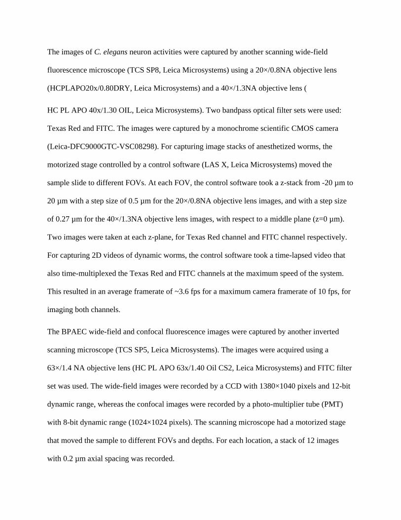
Fig. 1a demonstrates this concept by digitally propagating a single fluorescence image of a 300

nm fluorescent bead (excitation/emission: 538 nm/584 nm) to multiple user defined planes. The

native DOF of the input fluorescence image, defined by the NA of the objective lens (20×/0.75

NA), is ~ 1 µm; using Deep-Z, we were able to digitally refocus the image of this fluorescent

bead over an axial range of ~ ±10 µm, matching the mechanically-scanned corresponding images

of the same region of interest (ROI), which form the ground truth. Note that the PSF in Fig. 1a is

asymmetric in the axial direction, which provides directional cues to the neural network

regarding the digital propagation of an input image by Deep-Z. Unlike a symmetric Gaussian

beam27, such PSF asymmetry along the axial direction is ubiquitous in fluorescence microscopy

systems28. In addition to digitally refocusing an input fluorescence image, Deep-Z also provides

improved signal-to-noise ratio (SNR) at its output in comparison to a fluorescence image of the

same object measured at the corresponding depth (see Supplementary Fig. S1); at the heart of

this SNR increase compared to a mechanically-scanned ground truth is the ability of the neural

network to reject various sources of image noise that were not generalized during its training

phase. To further quantify Deep-Z output performance we used PSF analysis; Figs. 1b,c illustrate

the histograms of both the lateral and the axial full-width-half-maximum (FWHM) values of 461

individual/isolated nano-beads distributed over ~ 500 × 500 µm2. The statistics of these

histograms very well agree with each other (Fig. 1b,c), confirming the match between Deep-Z

output images calculated from a single fluorescence image (N=1 measured image) and the

corresponding axially-scanned ground truth images (N=41 measured images). This quantitative

match highlights the fact that Deep-Z indirectly learned, through image data, the 3D refocusing

of fluorescence light. However, this learned capability is limited to be within the axial range

determined by the training dataset (e.g., ±10 µm in this work), and fails outside of this training

range (see Supplementary Fig. S2 for quantification of this phenomenon).

Next, we tested the Deep-Z framework by imaging the neurons of a C. elegans nematode

expressing pan-neuronal tagRFP 29. Fig. 2 demonstrates our blind testing results for Deep-Z

based refocusing of different parts of a C. elegans worm from a single wide-field fluorescence

input image. Using Deep-Z, non-distinguishable fluorescent neurons in the input image were

brought into focus at different depths, while some other in-focus neurons at the input image got

out-of-focus and smeared into the background, according to their true axial positions in 3D; see

the cross-sectional comparisons to the ground truth mechanical scans provided in Fig. 2 (also see

Supplementary Fig. S3 for image difference analysis). For optimal performance, this Deep-Z was

specifically trained using C. elegans samples, to accurately learn the 3D PSF information

together with the refractive properties of the nematode body and the surrounding medium. Using

Deep-Z, we also generated (from a single 2D fluorescence image of a C. elegans worm) a virtual

3D stack (Video S1) and 3D visualization (Video S2) of the sample, over an axial range of ~ ±10

µm. Similar results were also obtained for a C. elegans imaged under a 40×/1.3NA objective

lens, where Deep-Z successfully refocused the input image over an axial range of ~ ±4 µm; see

Supplementary Fig. S4 for details.

Since Deep-Z can digitally reconstruct the image of an arbitrary plane within a 3D sample using

a single 2D fluorescence image, without sacrificing the inherent resolution, frame-rate or photon-

efficiency of the imaging system, it is especially useful for imaging dynamic biological samples.

To demonstrate this capability, we captured a video of four moving C. elegans worms, where

each frame of this fluorescence video was digitally refocused to various depths using Deep-Z.

This enabled us to create simultaneously running videos of the same sample volume, each one

being focused at a different depth (see Video S3). This unique capability enabled by Deep-Z not

only eliminates the need for mechanical axial scanning and related optical hardware, but also

significantly reduces phototoxicity or photobleaching within the sample to enable longitudinal

experiments. Furthermore, each one of these virtually created videos are by definition temporally

synchronized to each other (i.e., the frames at different depths have identical time stamps), which

is not possible with a scanning-based 3D imaging system due to the unavoidable time delay

between successive measurements of different parts of the sample volume. In addition to 3D

imaging of the neurons of a nematode, Deep-Z also works well to digitally refocus the images of

fluorescent samples that are spatially denser such as the mitochondria and F-actin structures

within bovine pulmonary artery endothelial cells (BPAEC); see Supplementary Fig. S5 for

examples of these results.

In our results reported so far, the blindly tested samples were inferred with a Deep-Z network

that was trained using the same type of sample and the same microscopy system. In the

Supplementary Information, under the sub-sections ‘Robustness of Deep-Z to changes in samples

and imaging systems’ as well as ‘Deep-Z virtual refocusing capability at lower image exposure’,

we evaluated the performance of Deep-Z under different scenarios, where a change in the test

data distribution is introduced in comparison to the training image set, such as e.g., (1) a different

type of sample is imaged, (2) a different microscopy system is used for imaging, and (3) a

different illumination power or SNR is used; also refer to Supplementary Figs. S10-12. Our

results and related analysis reveal the robustness of Deep-Z to some of these changes; however,

as a general recommendation to achieve the best performance with Deep-Z, the neural network

should be trained (from scratch or through transfer learning, which significantly expedites the

training process, as illustrated in Supplementary Figs. S11-12) using training images obtained

with the same microscope system and the same types of samples, as expected to be used at the

testing phase.

Sample drift-induced defocus compensation using Deep-Z

Deep-Z also enables the correction for sample drift induced defocus after the image is captured.

To demonstrate this, Video S4 shows a moving C. elegans worm recorded by a wide-field

fluorescence microscope with a 20×/0.8NA objective lens (DOF ~ 1 µm). The worm was

defocused ~ 2 – 10 µm from the recording plane. Using Deep-Z, we can digitally refocus each

frame of the input video to different planes up to 10 µm, correcting this sample drift induced

defocus (Video S4). Such a sample drift is conventionally compensated by actively monitoring

the image focus and correcting for it during the measurement, e.g., by using an additional

microscope8. Deep-Z, on the other hand, provides the possibility to compensate sample drift in

already-captured 2D fluorescence images.

3D functional imaging of C. elegans using Deep-Z

An important application of 3D fluorescence imaging is neuron activity tracking; for example

genetically modified animals that express different fluorescence proteins are routinely imaged

using a fluorescence microscope to reveal their neuron activity. To highlight the utility of Deep-

Z for tracking the activity of neurons in 3D, we recorded the fluorescence video of a C. elegans

worm at a single focal plane (z = 0 µm) at ~3.6 Hz for ~35 sec, using a 20×/0.8NA objective lens

with two fluorescence channels: FITC for neuron activity and Texas Red for neuron locations.

The input video frames were registered with respect to each other to correct for the slight body

motion of the worm between the consecutive frames (see the Methods for details). Then, each

frame at each channel of the acquired video were digitally refocused using Deep-Z to a series of

axial planes from -10 µm to 10 µm with 0.5 µm step size, generating a virtual 3D fluorescence

stack for each acquired frame. Video S5 shows a comparison of the recorded input video and a

video of the maximum intensity projection (MIP) along z for these virtual stacks. As can be seen

in this comparison, the neurons that are defocused in the input video can be clearly refocused on

demand at the Deep-Z output for both of the fluorescence channels. This enables accurate spatio-

temporal tracking of individual neuron activity in 3D from a temporal sequence of 2D

fluorescence images, captured at single focal plane.

To quantify the neuron activity using Deep-Z output images, we segmented voxels of each

individual neuron using the Texas Red channel (neuron locations), and tracked the change of the

fluorescence intensity, i.e., Δ𝐹(𝑡) = 𝐹(𝑡) − 𝐹0, in the FITC channel (neuron activity) inside each

neuron segment over time, where 𝐹(𝑡) is the neuron fluorescence emission intensity and 𝐹0 is its

time average; see Methods for details. A total of 155 individual neurons in 3D were isolated

using Deep-Z output images, as shown in Fig. 3b, where the color represents the depth (z

location) of each neuron; also see Video S6. For comparison, we also report in Supplementary

Fig. S14(b) the results of the same segmentation algorithm applied on just the input 2D image,

where 99 neurons were identified, without any depth information; see the Supplementary

Information for further analysis reported in the sub-section “C. elegans neuron segmentation

comparison”.

Fig. 3c plots the activities of the 70 most active neurons, which were grouped into clusters C1-

C3 based on their calcium activity pattern similarities (see Methods for details). The activities of

all of the 155 neurons inferred using Deep-Z are provided in Supplementary Fig. S6. Fig. 3c

reports that cluster C3 calcium activities increased at t = 14 s, whereas the activities of cluster C2

decreased at a similar time point. These neurons very likely correspond to the motor neurons

type A and B that promote backward and forward motion, respectively, which typically anti-

correlate with each other30. Cluster C1 features two cells that were comparatively larger in size,

located in the middle of the worm. These cells had three synchronized short spikes at t = 4, 17

and 32 sec. Their 3D positions and calcium activity pattern regularity suggest that they are either

neuronal or muscle cells of the defecation system that initiates defecation in regular intervals in

coordination with the locomotion system31.

We emphasize that all this 3D tracked neuron activity was in fact embedded in the input 2D

fluorescence image sequence acquired at a single focal plane within the sample, but could not be

readily inferred from it. Through the Deep-Z framework and its 3D refocusing capability to user

defined surfaces within the sample volume, the neuron locations and activities were accurately

tracked using a 2D microscopic time sequence, without the need for mechanical scanning,

additional hardware, or a trade-off of resolution or imaging speed.

Since Deep-Z generates temporally synchronized virtual image stacks through purely digital

refocusing, it can be used to match the imaging speed to the limit of the camera framerate, by

using e.g., the stream mode, which typically enables a short video of up to 100 frames per

second. To highlight this opportunity, we used the stream mode of the camera of a Leica SP8

microscope (see the Methods section for details) and captured two videos at 100 fps for

monitoring the neuron nuclei (under the Texas Red channel) and the neuron calcium activity

(under the FITC channel) of a moving C. elegans over a period of 10 sec, and used Deep-Z to

generate virtually refocused videos from these frames over an axial depth range of +/- 10 µm, as

shown in Video S7 and Video S8, respectively.

Deep-Z based aberration correction using spatially non-uniform DPMs

The results that we reported up to now used uniform DPMs in both the training phase and the

blind testing in order to refocus an input fluorescence image to different planes within the sample

volume. Here we emphasize that, even though Deep-Z was trained with uniform DPMs, in the

testing phase one can also use spatially non-uniform entries as part of a DPM to refocus an input

fluorescence image onto user-defined 3D surfaces. This capability enables digital refocusing of

the fluorescence image of a 3D surface onto another 3D surface, defined by the pixel mapping of

the corresponding DPM.

Such a unique capability can be useful, among many applications, for simultaneous auto-

focusing of different parts of a fluorescence image after the image capture, measurement or

assessment of the aberrations introduced by the optical system (and/or the sample) as well as for

correction of such aberrations by applying a desired non-uniform DPM. To exemplify this

additional degree-of-freedom enabled by Deep-Z, Fig. 4 demonstrates the correction of the

planar tilting and cylindrical curvature of two different samples, after the acquisition of a single

2D fluorescence image per object. Fig. 4a illustrates the first measurement, where the plane of a

fluorescent nano-bead sample was tilted by 1.5° with respect to the focal plane of the objective

lens (see Methods for details). As a result, the left and right sides of the acquired raw

fluorescence image (Fig. 4c) were blurred and the corresponding lateral FWHM values for these

nano-beads became significantly wider, as reported in Fig. 4e. By using a non-uniform DPM (see

Fig. 4b), which represents this sample tilt, Deep-Z can act on the blurred input image (Fig. 4c)

and accurately bring all the nano-beads into focus (Fig. 4d), even though it was only trained

using uniform DPMs. The lateral FWHM values calculated at the network output image became

monodispersed, with a median of ~ 0.96 µm (Fig. 4f), in comparison to a median of ~ 2.14 µm at

the input image. Similarly, Fig. 4g illustrates the second measurement, where the nano-beads

were distributed on a cylindrical surface with a diameter of ~7.2 mm. As a result, the measured

raw fluorescence image exhibited defocused regions as illustrated in Fig. 4i, and the FWHM

values of these nano-bead images were accordingly broadened (Fig. 4k), corresponding to a

median value of ~ 2.41 µm. On the other hand, using a non-uniform DPM that defines this

cylindrical surface (Fig. 4h), the aberration in Fig. 4i was corrected using Deep-Z (Fig. 4j), and

similar to the tilted sample case, the lateral FWHM values calculated at the network output

image once again became monodispersed, as desired, with a median of ~ 0.91 µm (Fig. 4l).

To evaluate the limitations of this technique, we quantified the 3D surface curvature that a DPM

can have without generating artifacts. For this, we used a series of DPMs that consisted of 3D

sinusoidal patterns with lateral periods of D = 1, 2, …, 256 pixels along the x-direction (with a

pixel size of 0.325 µm) and an axial oscillation range of 8 µm, i.e., a sinusoidal depth span of -1

µm to -9 µm with respect to the input plane. Each one of these 3D sinusoidal DPMs was

appended on an input fluorescence image that was fed into the Deep-Z network. The network

output at each sinusoidal 3D surface defined by the corresponding DPM was then compared

against the images that were interpolated in 3D using an axially-scanned z-stack with a scanning

step size of 0.5 µm, which formed the ground truth images that we used for comparison. As

summarized in Supplementary Fig. S7, the Deep-Z network can reliably refocus the input

fluorescence image onto 3D surfaces defined by sinusoidal DPMs when the period of the

modulation is > 100 pixels (i.e., > 32 µm in object space). For faster oscillating DPMs, with

periods smaller than 32 µm, the network output images at the corresponding 3D surfaces exhibit

background modulation at these high-frequencies and their harmonics as illustrated in the

spectrum analysis reported in Supplementary Fig. S7. These higher harmonic artifacts and the

background modulation disappear for lower frequency DPMs, which define sinusoidal 3D

surfaces at the output with a lateral period of > 32 µm and an axial range of 8 µm.

Cross-modality digital refocusing of fluorescence images: Deep-Z+

Deep-Z framework enables digital refocusing of out-of-focus 3D features in a wide-field

fluorescence microscope image to user-defined surfaces. The same concept can also be used to

perform cross-modality digital refocusing of an input fluorescence image, where the generator

network can be trained using pairs of input and label images captured by two different

fluorescence imaging modalities, which we term as Deep-Z+. After its training, the Deep-Z+

network learns to digitally refocus a single input fluorescence image acquired by a fluorescence

microscope to a user-defined target surface in 3D, but this time the output will match an image of

the same sample captured by a different fluorescence imaging modality at the corresponding

height/plane. To demonstrate this unique capability, we trained a Deep-Z+ network using pairs

of wide-field microscopy images (used as inputs) and confocal microscopy images at the

corresponding planes (used as ground truth labels) to perform cross-modality digital refocusing

(see the Methods for training details). Fig. 5 demonstrates our blind testing results for imaging

microtubule structures of BPAEC using this Deep-Z+ framework. As seen in Fig. 5, the trained

Deep-Z+ network digitally refocused the input wide field fluorescence image onto different axial

distances, while at the same time rejecting some of the defocused spatial features at the refocused

planes, matching the confocal images of the corresponding planes, which serve as our ground

truth. For instance, the microtubule structure at the lower left corner of a ROI in Fig. 5, which

was prominent at a refocusing distance of z = 0.34 µm, was digitally rejected by Deep-Z+ at a

refocusing distance of z = -0.46 µm since it became out-of-focus at this axial distance, matching

the corresponding image of the confocal microscope at the same depth. As demonstrated in Fig.

5, Deep-Z+ merges the sectioning capability of confocal microscopy with its image refocusing

framework. Fig. 5 also reports x-z and y-z cross-sections of the Deep-Z+ output images, where

the axial distributions of the microtubule structures are significantly sharper in comparison to the

axial scanning images of a wide-field fluorescence microscope, providing a very good match to

the cross-sections obtained with a confocal microscope, matching the aim of its training.

Discussion

We developed a unique framework (Deep-Z), powered by deep neural networks, that enables 3D

refocusing within a sample using a single 2D fluorescence image. This framework is non-

iterative and does not require hyperparameter tuning following its training stage. In Deep-Z, the

user can specify refocusing distances for each pixel in a DPM (following the axial range used in

the training), and the fluorescence image can be digitally refocused to the corresponding surface

through Deep-Z, within the transformation limits reported earlier in our Results section (see e.g.,

Supplementary Figs. S2 and S7). As illustrated in the Supplementary Information, the Deep-Z

framework is also robust to changes in the density of the fluorescent objects within the sample

volume (up to a limit, which is a function of the axial refocusing distance), the exposure time of

the input images, as well as the illumination intensity modulation (see Supplementary Figs.

S10,13,15-17 for detailed analyses). Because the distances are encoded in DPM and modeled as

a convolutional channel, we can train the network with uniform DPMs, which still permits us to

apply various non-uniform DPMs during the inference stage as reported in the Results section for

e.g., correcting the sample drift, tilt, curvature or other optical aberrations, which brings

additional degrees-of-freedom to the imaging system.

Deep learning has also been recently demonstrated to be very effective in performing

deconvolution to boost the lateral 32–37 and the axial 38,39 resolution in microscopy images. Deep-

Z network reported here is unique as it selectively deconvolves the spatial features that come into

focus through the digital refocusing process (see e.g. Supplementary Fig. S5), while convolving

other features that go out-of-focus, bringing the contrast to in-focus features, based on a user-

defined DPM. Through this Deep-Z framework, we bring the snapshot 3D refocusing capability

of coherent imaging and holography to incoherent fluorescence microscopy, without any

mechanical scanning, additional hardware components, or a trade-off of imaging resolution or

speed. This not only significantly boosts the imaging speed, but also reduces the negative effects

of photobleaching and phototoxicity on the sample. For a widefield fluorescence microscopy

experiment, where an axial image stack is acquired, the illumination excites the fluorophores

through the entire thickness of the specimen, and the total light exposure of a given point within

the sample volume is proportional to the number of imaging planes (Nz) that are acquired during

a single-pass z-stack. In contrast, Deep-Z only requires a single image acquisition step, if its axial

training range covers the sample depth. Therefore, this reduction, enabled by Deep-Z, in the

number of axial planes that need to be imaged within a sample volume directly helps to reduce

the photodamage to the sample (refer to Supplementary Fig. S18 and the Supplementary

Information, the sub-section titled “Reduced photodamage using Deep-Z” for details).

Finally, we should note that the retrievable axial range in this method depends on the SNR of the

recorded image, i.e., if the depth information carried by the PSF falls below the noise floor,

accurate inference will become a challenging task. To validate the performance of a pre-trained

Deep-Z network model under variable SNR, we tested the inference of Deep-Z under different

exposure conditions (Supplementary Fig. S10), revealing the robustness of its inference over a

broad range of image exposure times that were not included in the training data (refer to the

Supplementary Information, sub-section “Deep-Z virtual refocusing capability at lower image

exposure” for details). In our Results section, we demonstrated an enhancement of ~20× in the

DOF of a wide-field fluorescence image using Deep-Z. This axial refocusing range is in fact not

an absolute limit but rather a practical choice for our training data, and it may be further

improved through hardware modifications to the optical set-up by e.g., engineering the PSF in

the axial direction 7,15,40–42 (see Supplementary Video S10 for an experimental demonstration of

Deep-Z blind inference for a double-helix PSF). In addition to requiring extra hardware and

sensitive alignment/calibration, such approaches would also require brighter fluorophores, to

compensate for photon losses due to the insertion of additional optical components in the

detection path.

Methods

Sample preparation

The 300 nm red fluorescence nano-beads were purchased from MagSphere Inc. (Item # PSF-

300NM 0.3 UM RED), diluted by 5,000 times with methanol, and ultrasonicated for 15 minutes

before and after dilution to break down the clusters. For the fluorescent bead samples on a flat

surface and a tilted surface, a #1 coverslip (22×22 mm2, ~150 µm thickness) was thoroughly

cleaned and plasma treated. Then, a 2.5 µL droplet of the diluted bead sample was pipetted onto

the coverslip and dried. For the fluorescent bead sample on a curved (cylindrical) surface, a glass

tube (~ 7.2 mm diameter) was thoroughly cleaned and plasma treated. Then a 2.5 µL droplet of

the diluted bead sample was pipetted onto the outer surface of the glass tube and dried.

Structural imaging of C. elegans neurons was carried out in strain AML18. AML18 carries the

genotype wtfIs3 [rab-3p::NLS::GFP + rab-3p::NLS::tagRFP] and expresses GFP and tagRFP in

the nuclei of all the neurons 29. For functional imaging, we used the strain AML32, carrying

wtfIs5 [rab-3p::NLS::GCaMP6s + rab-3p::NLS::tagRFP]. The strains were acquired from the

Caenorhabditis Genetics Center (CGC). Worms were cultured on Nematode Growth Media

(NGM) seeded with OP50 bacteria using standard conditions 43. For imaging, worms were

washed off the plates with M9, and anaesthetized with 3 mM levamisole 44. Anaesthetized

worms were then mounted on slides seeded with 3% Agarose. To image moving worms, the

levamisole was omitted.

Two slides of multi-labeled bovine pulmonary artery endothelial cells (BPAEC) were acquired

from Thermo Fisher: FluoCells Prepared Slide #1 and FluoCells Prepared Slide #2. These cells

were labeled to express different cell structures and organelles. The first slide uses Texas Red for

mitochondria and FITC for F-actin structures. The second slide uses FITC for microtubules.

Fluorescence image acquisition

The fluorescence images of nano-beads, C. elegans structure and BPAEC samples were captured

by an inverted scanning microscope (IX83, Olympus Life Science) using a 20×/0.75NA

objective lens (UPLSAPO20X, Olympus Life Science). A 130W fluorescence light source (U-

HGLGPS, Olympus Life Science) was used at 100% output power. Two bandpass optical filter

sets were used: Texas Red and FITC. The bead samples were captured by placing the coverslip

with beads directly on the microscope sample mount. The tilted surface sample was captured by

placing the coverslip with beads on a 3D-printed holder, which creates a 1.5° tilt with respect to

the focal plane. The cylindrical tube surface with fluorescent beads was placed directly on the

microscope sample mount. These fluorescent bead samples were imaged using Texas Red filter

set. The C. elegans sample slide was placed on the microscope sample mount and imaged using

Texas Red filter set. The BPAEC slide was placed on the microscope sample mount and imaged

using Texas Red and FITC filter sets. For all the samples, the scanning microscope had a

motorized stage (PROSCAN XY STAGE KIT FOR IX73/83) that moved the samples to

different FOVs and performed image-contrast-based auto-focus at each location. The motorized

stage was controlled using MetaMorph® microscope automation software (Molecular Devices,

LLC). At each location, the control software autofocused the sample based on the standard

deviation of the image, and a z-stack was taken from -20 µm to 20 µm with a step size of 0.5 µm.

The image stack was captured by a monochrome scientific CMOS camera (ORCA-flash4.0 v2,

Hamamatsu Photonics K.K), and saved in non-compressed tiff format, with 81 planes and 2048

× 2048 pixels in each plane.

The images of C. elegans neuron activities were captured by another scanning wide-field

fluorescence microscope (TCS SP8, Leica Microsystems) using a 20×/0.8NA objective lens

(HCPLAPO20x/0.80DRY, Leica Microsystems) and a 40×/1.3NA objective lens (

HC PL APO 40x/1.30 OIL, Leica Microsystems). Two bandpass optical filter sets were used:

Texas Red and FITC. The images were captured by a monochrome scientific CMOS camera

(Leica-DFC9000GTC-VSC08298). For capturing image stacks of anesthetized worms, the

motorized stage controlled by a control software (LAS X, Leica Microsystems) moved the

sample slide to different FOVs. At each FOV, the control software took a z-stack from -20 µm to

20 µm with a step size of 0.5 µm for the 20×/0.8NA objective lens images, and with a step size

of 0.27 µm for the 40×/1.3NA objective lens images, with respect to a middle plane (z=0 µm).

Two images were taken at each z-plane, for Texas Red channel and FITC channel respectively.

For capturing 2D videos of dynamic worms, the control software took a time-lapsed video that

also time-multiplexed the Texas Red and FITC channels at the maximum speed of the system.

This resulted in an average framerate of ~3.6 fps for a maximum camera framerate of 10 fps, for

imaging both channels.

The BPAEC wide-field and confocal fluorescence images were captured by another inverted

scanning microscope (TCS SP5, Leica Microsystems). The images were acquired using a

63×/1.4 NA objective lens (HC PL APO 63x/1.40 Oil CS2, Leica Microsystems) and FITC filter

set was used. The wide-field images were recorded by a CCD with 1380×1040 pixels and 12-bit

dynamic range, whereas the confocal images were recorded by a photo-multiplier tube (PMT)

with 8-bit dynamic range (1024×1024 pixels). The scanning microscope had a motorized stage

that moved the sample to different FOVs and depths. For each location, a stack of 12 images

with 0.2 µm axial spacing was recorded.

Image pre-processing and training data preparation

Each captured image stack was first axially aligned using an ImageJ plugin named “StackReg”

45, which corrects the rigid shift and rotation caused by the microscope stage inaccuracy. Then an

extended depth of field (EDF) image was generated using another ImageJ plugin named

“Extended Depth of Field” 46. This EDF image was used as a reference image to normalize the

whole image stack, following three steps: (1) Triangular threshold47 was used on the image to

separate the background and foreground pixels; (2) the mean intensity of the background pixels

of the EDF image was determined to be the background noise and subtracted; (3) the EDF image

intensity was scaled to 0-1, where the scale factor was determined such that 1% of the

foreground pixels above the background were greater than one (i.e., saturated); and (4) each

image in the stack was subtracted by this background level and normalized by this intensity

scaling factor. For testing data without an image stack, steps (1) – (3) were applied on the input

image instead of the EDF image.

To prepare the training and validation datasets, on each FOV, a geodesic dilation 48 with fixed

thresholds was applied on fluorescence EDF images to generate a mask that represents the

regions containing the sample fluorescence signal above the background. Then, a customized

greedy algorithm was used to determine a minimal set of regions with 256 × 256 pixels that

covered this mask, with ~5% area overlaps between these training regions. The lateral locations

of these regions were used to crop images on each height of the image stack, where the middle

plane for each region was set to be the one with the highest standard deviation. Then 20 planes

above and 20 planes below this middle plane were set to be the range of the stack, and an input

image plane was generated from each one of these 41 planes. Depending on the size of the data

set, around 5-10 out of these 41 planes were randomly selected as the corresponding target plane,

forming around 150 to 300 image pairs. For each one of these image pairs, the refocusing

distance was determined based on the location of the plane (i.e. 0.5 µm times the difference from

the input plane to the target plane). By repeating this number, a uniform DPM was generated and

appended to the input fluorescence image. The final dataset typically contained ~ 100,000 image

pairs. This was randomly divided into a training dataset and a validation dataset, which took 85%

and 15% of the data respectively. During the training process, each data point was further

augmented five times by flipping or rotating the images by a random multiple of 90. The

validation dataset was not augmented. The testing dataset was cropped from separate

measurements with sample FOVs that do not overlap with the FOVs of the training and

validation data sets.

Deep-Z network architecture

The Deep-Z network is formed by a least square GAN (LS-GAN) framework 49, and it is

composed of two parts: a generator and a discriminator, as shown in Supplementary Fig. S8. The

generator is a convolutional neural network (CNN) inspired by the U-Net 50, and follows a

similar structure as in Ref. 51. The generator network consists of a down-sampling path and a

symmetric up-sampling path. In the down sampling path, there are five down-sampling blocks.

Each block contains two convolutional layers that map the input tensor xk to the output tensor

xk+1:

xk+1 = xk + ReLU[CONVk2{ReLU[CONVk1{xk}]}] (1)

where ReLU[.] stands for the rectified linear unit operation, and CONV{. } stands for the

convolution operator (including the bias terms). The subscript of CONV denotes the number of

channels in the convolutional layer; along the down-sampling path we have: k1 =

25, 72, 144, 288, 576 and k2 = 48, 96, 192, 384, 768 for levels k = 1, 2, 3, 4, 5, respectively.

The “+” sign in Eq. (S1) represents a residual connection. Zero padding was used on the input

tensor xk to compensate for the channel number mismatch between the input and output tensors.

The connection between two consecutive down-sampling blocks is a 2×2 max-pooling layer with

a stride of 2×2 pixels to perform a 2× down-sampling. The fifth down-sampling block connects

to the up-sampling path, which will be detailed next.

In the up-sampling path, there are four corresponding up-sampling blocks, each of which

contains two convolutional layers that map the input tensor yk+1 to the output tensor yk using:

yk = ReLU[CONVk4{ReLU[CONVk3{CAT(xk+1, yk+1)}]}] (2)

where the CAT(⋅) operator represents the concatenation of the tensors along the channel

direction, i.e. CAT(xk+1, yk+1) appends tensor xk+1 from the down-sampling path to the tensor

yk+1 in the up-sampling path at the corresponding level k+1. The number of channels in the

convolutional layers, denoted by k3 and k4, are k3 = 72, 144, 288, 576 and k4 =

48, 96, 192, 384 along the up-sampling path for k = 1, 2, 3, 4, respectively. The connection

between consecutive up-sampling blocks is an up-convolution (convolution transpose) block that

up-samples the image pixels by 2×. The last block is a convolutional layer that maps the 48

channels to one output channel (see Supplementary Fig. S8).

The discriminator is a convolutional neural network that consists of six consecutive

convolutional blocks, each of which maps the input tensor zi to the output tensor zi+1, for a

given level i:

zi+1 = LReLU[CONVi2{LReLU[CONVi1{zi}]}] (3)

where the LReLU stands for leaky ReLU operator with a slope of 0.01. The subscript of the

convolutional operator represents its number of channels, which are i1 =

48,96,192, 384, 768, 1536 and i2 = 96,192, 384, 768, 1536, 3072, for the convolution block

i = 1, 2, 3, 4, 5, 6, respectively.

After the last convolutional block, an average pooling layer flattens the output and reduces the

number of parameters to 3072. Subsequently there are fully-connected (FC) layers of size 3072 ×

3072 with LReLU activation functions, and another FC layer of size 3072 × 1 with a Sigmoid

activation function. The final output represents the discriminator score, which falls within (0, 1),

where 0 represents a false and 1 represents a true label.

All the convolutional blocks use a convolutional kernel size of 3 × 3 pixels, and replicate

padding of one pixel unless mentioned otherwise. All the convolutions have a stride of 1 × 1

pixel, except the second convolutions in Eq. (S3), which has a stride of 2 × 2 pixels to perform a

2× down-sampling in the discriminator path. The weights are initialized using the Xavier

initializer 52, and the biases are initialized to 0.1.

Training and testing of the Deep-Z network

The Deep-Z network learns to use the information given by the appended DPM to digitally

refocus the input image to a user-defined plane. In the training phase, the input data of the

generator G(. ) have the dimensions of 256 × 256 × 2, where the first channel is the fluorescence

image, and the second channel is the user-defined DPM. The target data of G(. ) have the

dimensions of 256 × 256, which represent the corresponding fluorescence image at a surface

specified by the DPM. The input data of the discriminator D(. ) have the dimensions of 256 ×

256, which can be either the generator output or the corresponding target z(i). During the training

phase, the network iteratively minimizes the generator loss LG and discriminator loss LD, defined

as:

LG =1

2N⋅∑[D(G(x(i))) − 1]

2N

i=1

+ α ⋅1

2N⋅∑MAE(x(i), z(i))

N

i=1

(4)

LD =1

2N⋅∑[D(G(x(i)))]

2N

i=1

+1

2N⋅∑[D(z(i)) − 1]

2N

i=1

(5)

where N is the number of images used in each batch (e.g., N = 20), G(x(i)) is the generator

output for the input x(i), z(i) is the corresponding target label, D(. ) is the discriminator, and

MAE(. ) stands for mean absolute error. α is a regularization parameter for the GAN loss and the

MAE loss in LG. In the training phase, it was chosen as α =0.02. For training stability and

optimal performance, adaptive momentum optimizer (Adam) was used to minimize both LG and

LD, with a learning rate of 10−4 and 3 × 10−5 for LG and LD respectively. In each iteration, six

updates of the generator loss and three updates of the discriminator loss were performed. The

validation set was tested every 50 iterations, and the best network (to be blindly tested) was

chosen to be the one with the smallest MAE loss on the validation set.

In the testing phase, once the training is complete, only the generator network is active. Limited

by the graphical memory of our GPU, the largest image FOV that we tested was 1536 × 1536

pixels. Because image was normalized to be in the range 0–1, whereas the refocusing distance

was on the scale of around -10 to 10 (in units of µm), the DPM entries were divided by 10 to be

in the range of -1 to 1 before the training and testing of the Deep-Z network, to keep the dynamic

range of the image and DPM matrices similar to each other.

The network was implemented using TensorFlow 53, performed on a PC with Intel Core i7-

8700K six-core 3.7GHz CPU and 32GB RAM, using an Nvidia GeForce 1080Ti GPU. On

average, the training takes ~ 70 hours for ~ 400,000 iterations (equivalent to ~ 50 epochs). After

the training, the network inference time was ~ 0.2 s for an image with 512 × 512 pixels and ~ 1s

for an image with 1536 × 1536 pixels on the same PC.

Measurement of the lateral and axial FWHM values of the fluorescent beads samples.

For characterizing the lateral FWHM of the fluorescent beads samples, a threshold was

performed on the image to extract the connected components. Then, individual regions of 30 ×

30 pixels were cropped around the centroid of these connected components. A 2D Gaussian fit

was performed on each of these individual regions, which was done using lsqcurvefit 54 in

Matlab (MathWorks, Inc) to match the function:

I(x, y) = A ⋅ exp [(x − xc)

2

2 ⋅ σx2+(y − yc)

2

2 ⋅ σy2] (6)

The lateral FWHM was then calculated as the mean FWHM of x and y directions, i.e.,

FWHMlateral = 2√2 ln 2 ⋅σx ⋅ Δx + σy ⋅ Δy

2 (7)

where Δx = Δ𝑦 = 0.325 𝜇𝑚 was the effective pixel size of the fluorescence image on the object

plane. A histogram was subsequently generated for the lateral FWHM values for all the

thresholded beads (e.g., n = 461 for Fig. 1 and n > 750 for Fig. 4).

To characterize the axial FWHM values for the bead samples, slices along the x-z direction with

81 steps were cropped at y = yc for each bead, from either the digitally refocused or the

mechanically-scanned axial image stack. Another 2D Gaussian fit was performed on each

cropped slice, to match the function:

I(x, z) = A ⋅ exp [(x − xc)

2

2 ⋅ σx2+(z − zc)

2

2 ⋅ σz2] (8)

The axial FWHM was then calculated as:

FWHMaxial = 2√2 ln 2 ⋅ σz ⋅ Δz (9)

where Δz = 0.5 𝜇𝑚 was the axial step size. A histogram was subsequently generated for the

axial FWHM values.

Image quality evaluation

The network output images Iout were evaluated with reference to the corresponding ground truth

images IGT using five different criteria: (1) mean square error (MSE), (2) root mean square error

(RMSE), (3) MAE, (4) correlation coefficient, and (5) SSIM 55. The MSE is one of the most

widely used error metrics, defined as:

MSE(Iout, IGT) =1

Nx ⋅ Ny‖Iout − IGT‖

2

2 (10)

where Nx and Ny represent the number of pixels in the x and y directions, respectively. The

square root of MSE results in RMSE. Compared to MSE, MAE uses 1-norm difference (absolute

difference) instead of 2-norm difference, which is less sensitive to significant outlier pixels:

MAE(Iout, IGT) =1

Nx ⋅ Ny‖Iout − IGT‖

1 (11)

The correlation coefficient is defined as:

corr(Iout, IGT) =∑ ∑ (Ixy

out − μout)(IxyGT − μGT)yx

√(∑ ∑ (Ixyout − μout)

2yx ) (∑ ∑ (Ixy

GT − μGT)2

yx )

(12)

where 𝜇𝑜𝑢𝑡 𝑎𝑛𝑑 𝜇𝐺𝑇 are the mean values of the images 𝐼𝑜𝑢𝑡 𝑎𝑛𝑑 𝐼𝐺𝑇 respectively.

While these criteria listed above can be used to quantify errors in the network output compared

to the GT, they are not strong indicators of the perceived similarity between two images. SSIM

aims to address this shortcoming by evaluating the structural similarity in the images, defined as:

SSIM(Iout, IGT) =(2μoutμGT + C1)(2σout,GT + C2)

(μout2 + μGT

2 + C1)(σout2 + σGT

2 + C2) (13)

where 𝜎𝑜𝑢𝑡 and 𝜎𝐺𝑇 are the standard deviations of 𝐼𝑜𝑢𝑡 𝑎𝑛𝑑 𝐼𝐺𝑇 respectively, and 𝜎𝑜𝑢𝑡,𝐺𝑇 is the

cross-variance between the two images.

Tracking and quantification of C. elegans neuron activity

The C. elegans neuron activity tracking video was captured by time-multiplexing the two

fluorescence channels (FITC, followed by TexasRed, and then FITC and so on). The adjacent

frames were combined so that the green color channel was FITC (neuron activity) and the red

color channel was Texas Red (neuron nuclei). Subsequent frames were aligned using a feature-

based registration toolbox with projective transformation in Matlab (MathWorks, Inc.) to correct

for slight body motion of the worms. Each input video frame was appended with DPMs

representing propagation distances from -10 µm to 10 µm with 0.5 µm step size, and then tested

through a Deep-Z network (specifically trained for this imaging system), which generated a

virtual axial image stack for each frame in the video.

To localize individual neurons, the red channel stacks (Texas Red, neuron nuclei) were projected

by median-intensity through the time sequence. Local maxima in this projected median intensity

stack marked the centroid of each neuron and the voxels of each neuron was segmented from

these centroids by watershed segmentation48, which generated a 3D spatial voxel mask for each

neuron. A total of 155 neurons were isolated. Then, the average of the 100 brightest voxels in the

green channel (FITC, neuron activity) inside each neuron spatial mask was calculated as the

calcium activity intensity 𝐹𝑖(𝑡), for each time frame t and each neuron 𝑖 = 1,2, … ,155. The

differential activity was then calculated, Δ𝐹(𝑡) = 𝐹(𝑡) − 𝐹0, for each neuron, where 𝐹0 is the

time average of 𝐹(𝑡).

By thresholding on the standard deviation of each Δ𝐹(𝑡), we selected the 70 most active cells

and performed further clustering on them based on their calcium activity pattern similarity

(Supplementary Fig. S6b) using a spectral clustering algorithm 56,57. The calcium activity pattern

similarity was defined as

Sij = exp

(

−

‖ΔFi(t)Fi0

−ΔFj(t)

Fj0‖

2

σ2

)

(14)

for neurons i and j, which results in a similarity matrix S (Supplementary Fig. S6c). σ = 1.5 is

the standard deviation of this Gaussian similarity function, which controls the width of the

neighbors in the similarity graph. The spectral clustering solves an eigen-value problem on the

graph Laplacian L generated from the similarity matrix S, defined as the difference of weight

matrix W and degree matrix D, i.e.,

L = D −W (15)

where

Wij = {Sij if i ≠ j

0 if i = j (16)

Dij = {∑Wijj

if i = j

0 if i ≠ j

(17)

The number of clusters was chosen using eigen-gap heuristics57, which was the index of the

largest general eigenvalue (by solving general eigen value problem 𝐿𝑣 = 𝜆𝐷𝑣) before the eigen-

gap, where the eigenvalues jump up significantly, which was determined to be k=3 (see

Supplementary Fig. S6d). Then the corresponding first k=3 eigen-vectors were combined as a

matrix, whose rows were clustered using standard k-means clustering57, which resulted in the

three clusters of the calcium activity patterns shown in Supplementary Fig. S6e and the

rearranged similarity matrix shown in Supplementary Fig. S6f.

Cross-modality alignment of wide-field and confocal fluorescence images

Each stack of the wide-field/confocal pair was first self-aligned and normalized using the method

described in the previous sub-section. Then the individual FOVs were stitched together using

“Image Stitching” plugin of ImageJ 58. The stitched wide-field and confocal EDF images were

then co-registered using a feature-based registration with projective transformation performed in

Matlab (MathWorks, Inc) 59. Then the stitched confocal EDF images as well as the stitched

stacks were warped using this estimated transformation to match their wide-field counterparts

(Supplementary Fig. S9a). The non-overlapping regions of the wide-field and warped confocal

images were subsequently deleted. Then the above-described greedy algorithm was used to crop

non-empty regions of 256 × 256 pixels from the remaining stitched wide-field images and their

corresponding warped confocal images. The same feature-based registration was applied on each

pair of cropped regions for fine alignment. This step provides good correspondence between the

wide field image and the corresponding confocal image in the lateral directions (Supplementary

Fig. S9b).

Although the axial scanning step size was fixed to be 0.2 µm, the reference zero-point in the

axial direction for the wide-field and the confocal stacks needed to be matched. To determine

this reference zero-point in the axial direction, the images at each depth were compared with the

EDF image of the same region using structural similarity index (SSIM) 55, providing a focus

curve (Supplementary Fig. S9c). A second order polynomial fit was performed on four points in

this focus curve with highest SSIM values, and the reference zero-point was determined to be the

peak of the fit (Supplementary Fig. S9c). The heights of wide-field and confocal stacks were

then centered by their corresponding reference zero-points in the axial direction. For each wide-

field image used as input, four confocal images were randomly selected from the stack as the

target, and their DPMs were calculated based on the axial difference of the centered height

values of the confocal and the corresponding wide-field images.

Code availability

Deep learning models reported in this work used standard libraries and scripts that are publicly

available in TensorFlow. Through a custom-written Fiji based plugin, we provided our trained

network models (together with some sample test images) for the following objective lenses:

Leica HC PL APO 20x/0.80 DRY (two different network models trained on TxRd and FITC

channels), Leica HC PL APO 40x/1.30 OIL (trained on TxRd channel), Olympus UPLSAPO20X

- 0.75 NA (trained on TxRd channel). We made this custom-written plugin and our models

publicly available through the following links:

http://bit.ly/deep-z-git

http://bit.ly/deep-z

Acknowledgments: The authors acknowledge Y. Luo, X. Tong, T. Liu, H. C. Koydemir and

Z.S. Ballard of UCLA, as well as Leica Microsystems for their help with some of the

experiments. The Ozcan Group at UCLA acknowledges the support of Koc Group, National

Science Foundation, and the Howard Hughes Medical Institute. Y.W. also acknowledges the

support of SPIE John Kiel scholarship. Some of the reported optical microscopy experiments

were performed at the Advanced Light Microscopy/Spectroscopy Laboratory and the Leica

Microsystems Center of Excellence at the California NanoSystems Institute at UCLA with

funding support from NIH Shared Instrumentation Grant S10OD025017 and NSF Major

Research Instrumentation grant CHE-0722519.

References:

1. Moerner, W. E. & Kador, L. Optical detection and spectroscopy of single molecules in a

solid. Phys. Rev. Lett. 62, 2535–2538 (1989).

2. Hell, S. W. & Wichmann, J. Breaking the diffraction resolution limit by stimulated emission:

stimulated-emission-depletion fluorescence microscopy. Opt. Lett. 19, 780–782 (1994).

3. Betzig, E. et al. Imaging Intracellular Fluorescent Proteins at Nanometer Resolution. Science

313, 1642–1645 (2006).

4. Hell, S. W. Far-Field Optical Nanoscopy. Science 316, 1153–1158 (2007).

5. Schrödel, T., Prevedel, R., Aumayr, K., Zimmer, M. & Vaziri, A. Brain-wide 3D imaging of

neuronal activity in Caenorhabditis elegans with sculpted light. Nat. Methods 10, 1013–1020

(2013).

6. Prevedel, R. et al. Simultaneous whole-animal 3D imaging of neuronal activity using light-

field microscopy. Nat. Methods 11, 727–730 (2014).

7. Tomer, R. et al. SPED Light Sheet Microscopy: Fast Mapping of Biological System

Structure and Function. Cell 163, 1796–1806 (2015).

8. Nguyen, J. P. et al. Whole-brain calcium imaging with cellular resolution in freely behaving

Caenorhabditis elegans. Proc. Natl. Acad. Sci. 113, E1074–E1081 (2016).

9. Siedentopf, H. & Zsigmondy, R. Uber sichtbarmachung und grö\s senbestimmung

ultramikoskopischer teilchen, mit besonderer anwendung auf goldrubingläser. Ann. Phys.

315, 1–39 (1902).

10. Lerner, T. N. et al. Intact-Brain Analyses Reveal Distinct Information Carried by SNc

Dopamine Subcircuits. Cell 162, 635–647 (2015).

11. Henriques, R. et al. QuickPALM: 3D real-time photoactivation nanoscopy image processing

in ImageJ. Nat. Methods 7, 339–340 (2010).

12. Abraham, A. V., Ram, S., Chao, J., Ward, E. S. & Ober, R. J. Quantitative study of single

molecule location estimation techniques. Opt. Express 17, 23352–23373 (2009).

13. Dempsey, G. T., Vaughan, J. C., Chen, K. H., Bates, M. & Zhuang, X. Evaluation of

fluorophores for optimal performance in localization-based super-resolution imaging. Nat.

Methods 8, 1027–1036 (2011).

14. Juette, M. F. et al. Three-dimensional sub–100 nm resolution fluorescence microscopy of

thick samples. Nat. Methods 5, 527–529 (2008).

15. Pavani, S. R. P. et al. Three-dimensional, single-molecule fluorescence imaging beyond the

diffraction limit by using a double-helix point spread function. Proc. Natl. Acad. Sci. 106,

2995–2999 (2009).

16. Levoy, M., Ng, R., Adams, A., Footer, M. & Horowitz, M. Light Field Microscopy. in ACM

SIGGRAPH 2006 Papers 924–934 (ACM, 2006). doi:10.1145/1179352.1141976

17. Pégard, N. C. et al. Compressive light-field microscopy for 3D neural activity recording.

Optica 3, 517–524 (2016).

18. Broxton, M. et al. Wave optics theory and 3-D deconvolution for the light field microscope.

Opt. Express 21, 25418–25439 (2013).

19. Cohen, N. et al. Enhancing the performance of the light field microscope using wavefront

coding. Opt. Express 22, 24817–24839 (2014).

20. Abrahamsson, S. et al. Fast multicolor 3D imaging using aberration-corrected multifocus

microscopy. Nat. Methods 10, 60–63 (2013).

21. Abrahamsson, S. et al. MultiFocus Polarization Microscope (MF-PolScope) for 3D

polarization imaging of up to 25 focal planes simultaneously. Opt. Express 23, 7734–7754

(2015).

22. Rosen, J. & Brooker, G. Non-scanning motionless fluorescence three-dimensional

holographic microscopy. Nat. Photonics 2, 190–195 (2008).

23. Brooker, G. et al. In-line FINCH super resolution digital holographic fluorescence

microscopy using a high efficiency transmission liquid crystal GRIN lens. Opt. Lett. 38,

5264–5267 (2013).

24. Siegel, N., Lupashin, V., Storrie, B. & Brooker, G. High-magnification super-resolution

FINCH microscopy using birefringent crystal lens interferometers. Nat. Photonics 10, 802–

808 (2016).

25. Goodfellow, I. et al. Generative Adversarial Nets. in Advances in Neural Information

Processing Systems 27 2672–2680 (2014).

26. Mirza, M. & Osindero, S. Conditional Generative Adversarial Nets. ArXiv14111784 Cs Stat

(2014).

27. Shaw, P. J. & Rawlins, D. J. The point-spread function of a confocal microscope: its

measurement and use in deconvolution of 3-D data. J. Microsc. 163, 151–165 (1991).

28. Kirshner, H., Aguet, F., Sage, D. & Unser, M. 3-D PSF fitting for fluorescence microscopy:

implementation and localization application. J. Microsc. 249, 13–25 (2013).

29. Nguyen, J. P., Linder, A. N., Plummer, G. S., Shaevitz, J. W. & Leifer, A. M. Automatically

tracking neurons in a moving and deforming brain. PLOS Comput. Biol. 13, e1005517

(2017).

30. Kato, S. et al. Global Brain Dynamics Embed the Motor Command Sequence of

Caenorhabditis elegans. Cell 163, 656–669 (2015).

31. Nagy, S., Huang, Y.-C., Alkema, M. J. & Biron, D. Caenorhabditis elegans exhibit a

coupling between the defecation motor program and directed locomotion. Sci. Rep. 5, 17174

(2015).

32. Rivenson, Y. et al. Deep learning microscopy. Optica 4, 1437–1443 (2017).

33. Ouyang, W., Aristov, A., Lelek, M., Hao, X. & Zimmer, C. Deep learning massively

accelerates super-resolution localization microscopy. Nat. Biotechnol. 36, 460–468 (2018).

34. Nehme, E., Weiss, L. E., Michaeli, T. & Shechtman, Y. Deep-STORM: super-resolution

single-molecule microscopy by deep learning. Optica 5, 458–464 (2018).

35. Rivenson, Y. et al. Deep Learning Enhanced Mobile-Phone Microscopy. ACS Photonics 5,

2354–2364 (2018).

36. Liu, T. et al. Deep learning-based super-resolution in coherent imaging systems. Sci. Rep. 9,

3926 (2019).

37. Wang, H. et al. Deep learning enables cross-modality super-resolution in fluorescence

microscopy. Nat. Methods 16, 103 (2019).

38. Weigert, M., Royer, L., Jug, F. & Myers, G. Isotropic reconstruction of 3D fluorescence

microscopy images using convolutional neural networks. ArXiv170401510 Cs (2017).

39. Zhang, X. et al. Deep learning optical-sectioning method. Opt. Express 26, 30762–30772

(2018).

40. Huang, B., Wang, W., Bates, M. & Zhuang, X. Three-Dimensional Super-Resolution

Imaging by Stochastic Optical Reconstruction Microscopy. Science 319, 810–813 (2008).

41. Antipa, N. et al. DiffuserCam: lensless single-exposure 3D imaging. Optica 5, 1–9 (2018).

42. Shechtman, Y., Sahl, S. J., Backer, A. S. & Moerner, W. E. Optimal Point Spread Function

Design for 3D Imaging. Phys. Rev. Lett. 113, 133902 (2014).

43. Brenner, S. The genetics of Caenorhabditis elegans. Genetics 77, 71–94 (1974).

44. C. elegans: Methods and Applications. (Humana Press, 2006).

45. Thevenaz, P., Ruttimann, U. E. & Unser, M. A pyramid approach to subpixel registration

based on intensity. IEEE Trans. Image Process. 7, 27–41 (1998).

46. Forster, B., Van De Ville, D., Berent, J., Sage, D. & Unser, M. Complex wavelets for

extended depth-of-field: a new method for the fusion of multichannel microscopy images.

Microsc. Res. Tech. 65, 33–42 (2004).

47. Zack, G. W., Rogers, W. E. & Latt, S. A. Automatic measurement of sister chromatid

exchange frequency. J. Histochem. Cytochem. 25, 741–753 (1977).

48. Gonzalez, R. C., Woods, R. E. & Eddins, S. L. Digital image processing using MATLAB.

(2004).

49. Mao, X. et al. Least squares generative adversarial networks. in Computer Vision (ICCV),

2017 IEEE International Conference on 2813–2821 (IEEE, 2017).

50. Ronneberger, O., Fischer, P. & Brox, T. U-Net: Convolutional Networks for Biomedical

Image Segmentation. in Medical Image Computing and Computer-Assisted Intervention –

MICCAI 2015 234–241 (2015). doi:10.1007/978-3-319-24574-4_28

51. Wu, Y. et al. Extended depth-of-field in holographic imaging using deep-learning-based

autofocusing and phase recovery. Optica 5, 704–710 (2018).

52. Glorot, X. & Bengio, Y. Understanding the difficulty of training deep feedforward neural

networks. in Proceedings of the Thirteenth International Conference on Artificial

Intelligence and Statistics 249–256 (2010).

53. Abadi, M. et al. TensorFlow: A System for Large-Scale Machine Learning. in OSDI 16,

265–283 (2016).

54. Solve nonlinear curve-fitting (data-fitting) problems in least-squares sense - MATLAB

lsqcurvefit. Available at: https://www.mathworks.com/help/optim/ug/lsqcurvefit.html.

(Accessed: 21st November 2018)

55. Wang, Z., Bovik, A. C., Sheikh, H. R. & Simoncelli, E. P. Image quality assessment: from

error visibility to structural similarity. IEEE Trans. Image Process. 13, 600–612 (2004).

56. Shi, J. & Malik, J. Normalized Cuts and Image Segmentation. IEEE Trans Pattern Anal

Mach Intell 22, 888–905 (2000).

57. von Luxburg, U. A tutorial on spectral clustering. Stat. Comput. 17, 395–416 (2007).

58. Image Stitching. ImageJ Available at: https://imagej.net/Image_Stitching. (Accessed: 26th

November 2018)

59. Detect SURF features and return SURFPoints object - MATLAB detectSURFFeatures.

Available at: https://www.mathworks.com/help/vision/ref/detectsurffeatures.html.

(Accessed: 26th November 2018)

Fig. 1. Refocusing of fluorescence images using Deep-Z. (a) By concatenating a digital

propagation matrix (DPM) to a single fluorescence image, and running the resulting image

through a trained Deep-Z network, digitally refocused images at different planes can be rapidly

obtained, as if an axial scan is performed at the corresponding planes within the sample volume.

The DPM has the same size as the input image and its entries represent the axial propagation

distance for each pixel and can also be spatially non-uniform. The results of Deep-Z inference

are compared against the images of an axial-scanning fluorescence microscope for the same

fluorescent bead (300 nm), providing a very good match. (b) Lateral FWHM histograms for 461

individual/isolated fluorescence nano-beads (300 nm) measured using Deep-Z inference (N=1

captured image) and the images obtained using mechanical axial scanning (N=41 captured

images) provide a very good match to each other. (c) Same as in (b), except for the axial FWHM

measurements for the same data set, also revealing a very good match between Deep-Z inference

results and the axial mechanical scanning results.

Fig. 2. 3D imaging of C. Elegans neuron nuclei using Deep-Z. Different ROIs are digitally

refocused using Deep-Z to different planes within the sample volume; the resulting images

provide a very good match to the corresponding ground truth images, acquired using a scanning

fluorescence microscope. The absolute difference images of the input and output with respect to

the corresponding ground truth image are also provided on the right, with structural similarity

index (SSIM) and root mean square error (RMSE) values reported, further demonstrating the

success of Deep-Z. Scale bar: 25 µm.

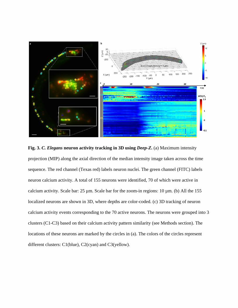
Fig. 3. C. Elegans neuron activity tracking in 3D using Deep-Z. (a) Maximum intensity

projection (MIP) along the axial direction of the median intensity image taken across the time

sequence. The red channel (Texas red) labels neuron nuclei. The green channel (FITC) labels

neuron calcium activity. A total of 155 neurons were identified, 70 of which were active in

calcium activity. Scale bar: 25 µm. Scale bar for the zoom-in regions: 10 µm. (b) All the 155

localized neurons are shown in 3D, where depths are color-coded. (c) 3D tracking of neuron

calcium activity events corresponding to the 70 active neurons. The neurons were grouped into 3

clusters (C1-C3) based on their calcium activity pattern similarity (see Methods section). The

locations of these neurons are marked by the circles in (a). The colors of the circles represent

different clusters: C1(blue), C2(cyan) and C3(yellow).

Fig. 4. Non-uniform DPMs enable digital refocusing of a single fluorescence image onto

user-defined 3D surfaces using Deep-Z. (a) Measurement of a tilted fluorescent sample (300

nm beads). (b) The corresponding DPM for this tilted plane. (c) Measured raw fluorescence

image; the left and right parts are out-of-focus in different directions, due to the sample tilt. (d)

The Deep-Z output rapidly brings all the regions into correct focus. (e,f) report the lateral

FWHM values of the nano-beads shown in (c,d), respectively, clearly demonstrating that Deep-Z

with the non-uniform DPM brought the out-of-focus particles into focus. (g) Measurement of a

cylindrical surface with fluorescent beads (300 nm beads). (h) The corresponding DPM for this

curved surface. (i) Measured raw fluorescence image; the middle region and the edges are out-

of-focus due to the curvature of the sample. (j) The Deep-Z output rapidly brings all the regions

into correct focus. (k,l) report the lateral FWHM values of the nano-beads shown in (i,j),

respectively, clearly demonstrating that Deep-Z with the non-uniform DPM brought the out-of-

focus particles into focus.

Fig. 5. Deep-Z+: Cross-modality digital refocusing of fluorescence images. A single wide-

field fluorescence image (63×/1.4NA objective lens) of BPAEC microtubule structures (a) was

digitally refocused using Deep-Z+ to different planes in 3D (b), matching the images captured by

a confocal microscope at the corresponding planes (c), retrieving volumetric information from a

single input image and performing axial sectioning at the same time. Wide-field (WF) images are

also shown in (c) for comparison. These scanning WF images report the closest heights to the

corresponding confocal images, and have 60 nm axial offset since the two image stacks are

discretely scanned and digitally aligned to each other. x-z and y-z cross-sections of the refocused

images are also shown to demonstrate the match between Deep-Z+ inference and the ground

truth confocal microscope images of the same planes; the same cross-sections (x-z and y-z) are

also shown for a wide-field scanning fluorescence microscope, reporting a significant axial blur

in each case. Each cross-sectional zoomed-in image spans 1.6 µm in z-direction (with an axial

step size of 0.2 µm), and the dotted arrows mark the locations, where the x-z and y-z cross-

sections were taken. (d) The absolute difference images of the Deep-Z+ output with respect to

the corresponding confocal images are also provided, with SSIM and RMSE values, further

quantifying the performance of Deep-Z+. For comparison, we also show the absolute difference

images of the ‘standard’ Deep-Z output images as well as the scanning wide-field fluorescence

microscope images with respect to the corresponding confocal images, both of which report

increased error and weaker SSIM compared to |GT - Deep-Z+|. The quantitative match between

|GT - WF| and |GT - Deep-Z| (see d) also suggests that the impact of 60 nm axial offset between

the confocal and wide-field image stacks is negligible. Scale bar: 10 µm.