
Three Dimensional Vibration Analysis Thesis 2009 Tmm&Ansys
187
ÇUKUROVA UNIVERSITY INSTITUTE OF NATURAL AND APPLIED SCIENCES PhD THESIS Ahmet ÖZBAY THREE DIMENSIONAL VIBRATION ANALYSIS OF LIQUID-FILLED PIPING SYSTEMS DEPARTMENT OF MECHANICAL ENGINEERING ADANA, 2009
description
vibration
Transcript of Three Dimensional Vibration Analysis Thesis 2009 Tmm&Ansys
ÇUKUROVA UNIVERSITY
INSTITUTE OF NATURAL AND APPLIED SCIENCES
PhD THESIS
Ahmet ÖZBAY
THREE DIMENSIONAL VIBRATION ANALYSIS
OF LIQUID-FILLED PIPING SYSTEMS
DEPARTMENT OF MECHANICAL ENGINEERING
ADANA, 2009

ÇUKUROVA ÜNİVERSİTESİ
FEN BİLİMLERİ ENSTİTÜSÜ
THREE DIMENSIONAL VIBRATION ANALYSIS OF LIQUID-FILLED PIPING SYSTEMS
Ahmet ÖZBAY
DOKTORA TEZİ
MAKİNA MÜHENDİSLİĞİ ANABİLİM DALI
Bu Tez ..../..../2009 Tarihinde Aşağıdaki Jüri Üyeleri Tarafından
Oybirliği/Oyçokluğu İle Kabul Edilmiştir.
İmza: …………………… İmza: …………………………. İmza: …………………………
Prof. Dr. Vebil YILDIRIM Prof. Dr. Naki TÜTÜNCÜ Doç. Dr. H. Murat Arslan
DANIŞMAN ÜYE ÜYE
İmza: ………………………
İmza: …………………
Doç. Dr. Ahmet PINARBAŞI Yrd.Doç. Dr. İbrahim KELEŞ
ÜYE ÜYE
Bu Tez Enstitümüz Makina Mühendisliği Anabilim Dalında Hazırlanmıştır.
Kod No:
Prof. Dr. Aziz ERTUNÇ Enstitü Müdürü
Not: Bu tezde kullanılan özgün ve başka kaynaktan yapılan bildirişlerin, çizelge, şekil ve fotoğrafların kaynak gösterilmeden kullanımı, 5846 sayılı Fikir ve Sanat Eserleri Kanunundaki hükümlere tabidir.

I
ABSTRACT
PhD THESIS
THREE DIMENSIONAL VIBRATION ANALYSIS OF LIQUID-FILLED PIPING SYSTEMS
Ahmet ÖZBAY
DEPARTMENT OF MECHANICAL ENGINEERING INSTITUTE OF NATURAL AND APPLIED SCIENCES
UNIVERSITY OF ÇUKUROVA
Supervisor
Year
: Prof. Dr. Vebil YILDIRIM
: 2009, Pages: 164
Jury : Prof. Dr. Vebil YILDIRIM
Prof. Dr. Naki TÜTÜNCÜ
Doç. Dr. H. Murat Arslan
Doç. Dr. Ahmet PINARBAŞI
Yrd.Doç. Dr. İbrahim KELEŞ
In the theoretical part of this work, the transfer matrix method (TMM) is employed
to study the free vibration analysis of liquid-filled (air/water) piping systems. The existing
governing equations which consist of a set of fourteen linear differential equations of first
degree are considered. Fixed-fixed and fixed-free ends are studied with five different basic
geometries of piping systems made of either copper or steel, such as single-span, L-bend, Z-
bend, U-bend and 3-D bend. A few experiments are also completed to support the theoretical
solutions. The effect of the elastic foundation on the natural frequencies is also studied.
Finally, a parametric study is carried out to understand correctly the vibrational behavior of
such systems. Present results are verified with the frequencies available in the literature.
Keywords:
Flow-Induced Vibration, Transfer Matrix Method, Three Dimensional Vibration Analysis, Liquid-Filled.
ITD
Highlight
ITD
Highlight
ITD
Highlight

II
ÖZ
DOKTORA TEZİ
AKIŞKAN TAŞIYAN BORU HATLARININ ÜÇ BOYUTLU TİTREŞİM ANALİZİ
Ahmet ÖZBAY
ÇUKUROVA ÜNİVERSİTESİ FEN BİLİMLERİ ENSTİTÜSÜ
MAKİNA MÜHENDİSLİĞİ ANABİLİM DALI
Danışman Yıl
: Prof. Dr. Vebil YILDIRIM
: 2008, Pages: 164
Jüri : Prof. Dr. Vebil YILDIRIM
Prof. Dr. Naki TÜTÜNCÜ
Doç. Dr. H. Murat Arslan
Doç. Dr. Ahmet PINARBAŞI
Yrd.Doç. Dr. İbrahim KELEŞ
Bu çalışmanın teorik kısmında, akışkan (hava/su) dolu boru
sistemlerinin serbest titreşim analizi için taşıma matrisi yöntemi (TMM)
kullanılmıştır. Literatürde mevcut on dört adet lineer birinci dereceden diferansiyel
denklemden oluşan denklem takımı göz önüne alınmıştır. Ankastre-ankastre ve
ankastre-serbest uçlar için, tek açıklıklı, L, Z, U ve üç boyutlu konfigürasyonlardan
oluşan bakır/çelik malzemeden yapılmış boru sistemleri ele alınmıştır. Teorik
sonuçları desteklemek amacı ile bazı deneyler gerçekleştirilmiştir. Elastik zemin
etkisi ayrıca çalışılmıştır. Son olarak parametrik bir çalışma gerçekleştirilmiştir. Bu
çalışmadan elde edilen sonuçlar, literatürde bulunan frekanslarla doğrulanmıştır.
Anahtar Kelimeler: Akış Kaynaklı Titreşim, Transfer Matris Metodu, Üç
Boyutlu Titreşim Analizi, Akışkan Dolu.

III
ACKNOWLEDGEMENTS
I am truly grateful to my research supervisor, Prof. Dr. Vebil YILDIRIM,
for his invaluable guidance and support throughout the preparation of this thesis and
during my graduate education.
I would like to express my special thanks to Advisory Committee Members,
Prof. Dr. Naki TÜTÜNCÜ, Assoct. Prof. Dr. Ahmet PINARBAŞI and Assoct. Prof.
Dr. H. Murat ARSLAN, for their devotion of invaluable time throughout my research
activities.
I would like to offer my cordial thanks to Assist. Prof. Dr. İbrahim KELEŞ
who have improved my morale with their encouraging advises during my thesis
study.
I would like to thank to all my research assistant friends at our Mechanical
Engineering Department and Colleague in Mersin Soda Ash Plant for their
continuous support and motivation.
Another point that should be emphasized here is the continuous moral
support, motivation, encouragement and patience of my wife Fügen ÖZBAY, my
daughter Derin ÖZBAY, and my family throughout my scientific efforts.

IV
CONTENTS
PAGE
ABSTRACT.…………………………………………...…………………....... I
ÖZ …………………………………………………………………................. II
ACKNOWLEDGEMENTS………………………………………………...… III
CONTENTS…………………………………………………........................... IV
LIST OF TABLES .…………………………………………………………... VII
LIST OF FIGURES…………………………………………………………... XII
NOMENCLATURE……………………………………………….................. XVIII
1. INTRODUCTION……………………………………………………….. 1
2. LITERATURE REVIEW........................................................................... 2
2.1. Flow Induced Vibrations in Pipelines ………………………………. 2
2.2. Transfer Matrix Method........……......………..................................... 8
3. MATERIAL AND METHOD.................................................................... 10
3.1. Material.................................................................................... 10
3.1.1. Pipe Materials................................................................... 11
3.1.2. Liquid …………………………………………………... 12
3.1.3. External Shaker ………………………………………… 12
3.1.4. Transducers....................................................................... 13
3.2. Method............................................................................................ 14
3.2.1. Governing Differential Equations ………….................... 14
3.2.1.1. Axial Vibration – Liquid and Pipe Wall …….… 15
3.2.1.2. Transverse Vibration in x-z Plane ……………. 27
3.2.1.3. Transverse Vibration in y-z Plan ……………... 33
3.2.1.4. Torsional Vibration …………………………... 34
3.2.2. Transfer Matrix Method.................................................... 38
3.2.2.1. Transfer Matrix Procedure ……………...……... 38
3.2.2.2. Field Transfer Matrices........................................ 42
3.2.2.2.(1). Liquid and Pipe Wall Vibration …................ 43
3.2.2.2.(2). Transverse Vibration in x-z Plane.................. 45
3.2.2.2.(3). Transverse Vibration in y-z Plane.................. 45
ITD
Highlight
ITD
Highlight
V
3.2.2.2.(4). Torsional Vibration about z Axis ...………... 47
3.2.2.3. General Field Transfer Matrix............................. 47
3.2.2.4. Point Matrices...................................................... 49
3.2.2.4.(1). Bend Point Matrix.......................................... 49
3.2.2.4.(2). Spring Point Matrix........................................ 54
3.2.2.5. Boundary Conditions........................................... 56
3.2.2.6. Natural Frequencies............................................. 58
3.2.2.7. Vibration of a Pipe on Elastic Foundation .......... 59
4. RESULTS AND DISCUSSION................................................................. 60
4.1. Single Span Pipe with Various Conditions ……………………… 63
4.1.1. Fixed-Fixed Single Span Pipe ………………….…….… 64
4.1.2. Fixed-Free Single Span Pipe ………………….…….….. 69
4.1.3. Single Span Pipe with Rigid Support ………………….. 72
4.2. Two Pipe with 90 Degree Bend .………………………………… 74
4.2.1. L Bend with Fixed-Free End Conditions ………………. 75
4.2.2. L Bend with Fixed-Fixed End Conditions …………… 78
4.2.3. L Bend with Intermediate Conditions…………………... 89
4.3. Three Pipes in a Plane…………………………………………… 90
4.3.1. Z Bend with Fixed-Free End Conditions……………….. 90
4.3.2. Z Bend with Fixed-Fixed End Conditions……………… 92
4.3.3. U Bend with Fixed-Free End Conditions ……………… 102
4.3.4. U Bend with Fixed-Fixed End Conditions …………….. 103
4.4. Three Pipes in Two Planes ………………………………………. 115
4.4.1. 3D Bend with Fixed-Free End Conditions ……………. 115
4.4.2. 3D Bend with Fixed-Fixed End Conditions …………... 117
4.5. Elastic Foundation ………………………………………………. 125
4.5.1. Free Ended Single Span Pipe on an Elastic Foundation . 126
4.5.2. L Bend Free Ended Pipe on an Elastic Foundation …… 129
4.5.3. 3D Bend Free Ended Pipe on an Elastic Foundation … 132
4.6. Parametric Studies ……………………………………………… 135
4.6.1. Effect of Slenderness Ratio on the Natural Frequencies.. 135

VI
4.6.2. Effect of The Bend-Angle on The Natural Frequencies
of Planar Piping System……………………………….
148
5. CONCLUSIONS ……………………………………………………… 157
REFERENCES…………………………………………………….................. 159
CURRICULUM VITAE……………………………………………………… 162
APPENDIX ……………...……………………………………………………… 163

VII
LIST OF TABLES PAGE Table 3.1. Physical Properties of Copper Pipe ………………………… 11
Table 3.2. Physical Properties of Steel Pipe …………………………… 12
Table 3.3. Physical Properties of Liquid ………………………………. 12
Table 4.1. Comparison of the present theoretical natural frequencies
(rad/s) of 5m-length copper pipe filled by the air with the
literature(Fixed-Fixed and Open-Closed) ……………...……. 61
Table 4.2. Comparison of the present theoretical natural frequencies
(rad/s) of 5m-length copper pipe filled by the air with the
literature (Fixed-Fixed and Open-Closed) ..…...…………….. 61
Table 4.3. Natural frequencies (Hz) of 2m-length copper pipe with the
air (Fixed-Fixed and Open-Closed) ………………………… 65
Table 4.4. Natural frequencies (Hz) of 2m-length copper pipe with the
water (Fixed-Fixed and Open-Closed) ……………………… 68
Table 4.5. Natural frequencies (Hz) of 3.5m-length steel pipe with the
air (Fixed-Fixed and Open-Closed) …….…………………… 70
Table 4.6. Natural frequencies (Hz) of 3.5m-length steel pipe with the
water (Fixed-Fixed and Open-Closed) ……………………… 70
Table 4.7. Natural frequencies (Hz) of 3m-length copper pipe with the
air (Fixed-Free and Open-Closed) …………………………. 71
Table 4.8. Natural frequencies (Hz) of 3m-length copper pipe with the
water (Fixed-Free and Open-Closed) ….…………………… 71
Table 4.9. Natural frequencies (Hz) of 3m-length steel pipe with the air
(Fixed-Free and Open-Closed) …………………………….. 71
Table 4.10. Natural frequencies (Hz) of 3m-length steel pipe with the
water (Fixed-Free and Open-Closed) .………………………. 72
Table 4.11. Natural frequencies (Hz) of 7m-length copper pipe filled by
the air for intermediate rigid support (Fixed-Fixed and Open-
Closed) . …………………………………………………. 73
Table 4.12. Natural frequencies (Hz) of 7m-length copper pipe filled by 73

VIII
the water for intermediate rigid support (Fixed-Fixed and
Open-Closed) ………………………………………………..
Table 4.13. Natural frequencies (Hz) of 6m-length steel pipe filled by the
air for intermediate rigid support (Fixed-Fixed and Open-
Closed) ……………………….……………………………... 74
Table 4.14. Natural frequencies (Hz) of 6m-length steel pipe filled by the
water for intermediate rigid support (Fixed-Fixed and Open-
Closed) …………………………….………………………… 74
Table 4.15. Natural frequencies (Hz) of L-bended steel pipe with the air
(Fixed-Closed / Free-Closed) ……………………………….. 76
Table 4.16. Natural frequencies (Hz) of L-bended steel pipe with the
water (Fixed-Closed / Free-Closed) …………………………. 76
Table 4.17. Natural Frequencies (Hz) of L-bended copper pipe with the
air (Fixed-Closed / Free-Closed) …………………………….. 77
Table 4.18. Natural Frequencies (Hz) of L-bended copper pipe with the
water (Fixed-Closed / Free-Closed) ………………………… 77
Table 4.19. Natural frequencies (Hz) of L-bended steel pipe with the air
(Fixed-Open/ Fixed-Closed) (L1 = L2 = 2.4 m) …………….. 78
Table 4.20. Natural frequencies (Hz) of L-bended steel pipe with the
water (Fixed-Open/ Fixed-Closed) (L1 = L2 = 2.4 m) ………. 81
Table 4.21. Natural frequencies (Hz) of L-bended copper pipe with the
air (Fixed-Open/ Fixed-Closed) (L1 = L2 = 1 m) ……..…….. 84
Table 4.22. Natural frequencies (Hz) of L-bended copper pipe with the
water (Fixed-Open/ Fixed-Closed) (L1 = L2 = 1 m) ..……….. 86
Table 4.23. Natural frequencies (Hz) of L-bended copper pipe with the
air (Fixed-Open/ Fixed-Closed) (L1 = L2 = 3.5 m) ..………... 87
Table 4.24. Natural frequencies (Hz) of L-bended copper pipe with the
water (Fixed-Open/ Fixed-Closed) (L1 = L2 = 3.5 m) .…….. 88
Table 4.25. Natural frequencies of L-bended copper pipe filled by the
water with intermediate rigid supports (Fixed-Open/ Fixed-
Closed) …………………………………….………………… 89

IX
Table 4.26. Natural frequencies (Hz) of Z-bended steel pipe with the air
(Fixed-Closed / Free-Closed) (L1 = L2 = L3=1.25m) ……...... 93
Table 4.27. Natural frequencies (Hz) of Z-bended steel pipe with the
water (Fixed-Closed / Free-Closed) (L1 = L2 = L3=1.25m) ..... 93
Table 4.28. Natural frequencies (Hz) of Z-bended steel pipe with the air
(Fixed-Open/ Fixed-Closed) (L1 = L2 = L3=1.25m) ….......... 94
Table 4.29. Natural frequencies (Hz) of Z-bended steel pipe with the
water (Fixed-Open/ Fixed-Closed) (L1 = L2 = L3=1.25m) ...... 96
Table 4.30. Natural frequencies (Hz) of Z-bended copper pipe with the
air (Fixed-Open/ Fixed-Closed) (L1 = L2 = L3=1m) ….……... 98
Table 4.31. Natural Frequencies (Hz) of Z-bended copper pipe with the
water (Fixed-Open/ Fixed-Closed) (L1 = L2 = L3=1m)……… 101
Table 4.32. Natural Frequencies (Hz) of Z-bended copper pipe with the
air (Fixed-Open/ Fixed-Closed) (L1 = L2 = L3=7/3m=2.33m) 102
Table 4.33. Natural Frequencies (Hz) of Z-bended copper pipe with the
water (Fixed-Open/ Fixed-Closed) (L1 = L2 = L3=2.333m) 103
Table 4.34. Natural Frequencies (Hz) of U-bended steel pipe with the air
(Fixed-Open/ Free-Closed) (L1 = L2 = L3=1.25m) ..……….... 105
Table 4.35. Natural Frequencies (Hz) of U-bended steel pipe with the
water (Fixed-Open / Free-Closed) (L1 = L2 = L3=1.25m)….... 105
Table 4.36. Natural Frequencies (Hz) of U-bended steel pipe with the air
(Fixed-Open / Fixed-Closed) (L1 = L2 = L3=1.25m) …..….... 106
Table 4.37. Natural Frequencies (Hz) of U-bended steel pipe with the
water (Fixed-Open / Fixed-Closed) (L1 = L2 = L3=1.25m)….. 108
Table 4.38. Natural Frequencies (Hz) of U-bended cooper pipe with the
air (Fixed-Open / Fixed-Closed) (L1 = L2 = L3=1m)………… 109
Table 4.39. Natural Frequencies (Hz) of U-bended cooper pipe with the
water (Fixed-Open / Fixed-Closed) (L1 = L2 = L3=1m) ..…… 111
Table 4.40. Natural Frequencies (Hz) of U-bended cooper pipe with the
air (Fixed-Open / Fixed-Closed) (L1 = L2 = L3=2.333m) ….... 112
X
Table 4.41. Natural Frequencies (Hz) of U-bended cooper pipe with the
air (Fixed-Open / Fixed-Closed) (L1 = L2 = L3=2.333m) ….. 113
Table 4.42. Natural Frequencies (Hz) of 3D-bended steel pipe with the
air (Fixed-Open / Free-Closed) (L1 = L2 = L3=1.25m) ……… 116
Table 4.43. Natural Frequencies (Hz) of 3D-bended steel pipe with the
water (Fixed-Open / Free-Closed) (L1 = L2 = L3=1.25m) …... 116
Table 4.44. Natural Frequencies (Hz) of 3D-bended steel pipe with the
air (Fixed-Open / Fixed-Closed) (L1 = L2 = L3=1.25m) .……. 117
Table 4.45. Natural Frequencies (Hz) of 3D-bended steel pipe with the
water (Fixed-Open / Fixed-Closed) (L1 = L2 = L3=1.25m)…. 118
Table 4.46. Natural Frequencies (Hz) of 3D-bended copper pipe with the
air (Fixed-Open / Fixed-Closed) (L1 = L2 = L3=1m) ……….. 120
Table 4.47. Natural Frequencies (Hz) of 3D-bended copper pipe with the
water (Fixed-Open / Fixed-Closed) (L1 = L2 = L3=1m) ….… 121
Table 4.48. Natural Frequencies (Hz) of 3D-bended copper pipe with the
air (Fixed-Open / Fixed-Closed) (L1 = L2 = L3=2.333m) ….. 122
Table 4.49. Natural Frequencies (Hz) of 3D-bended copper pipe with the
water (Fixed-Open / Fixed-Closed) (L1 = L2 = L3=2.333m) .. 123
Table 4.50. Natural Frequencies (Hz) of 6m length free ended steel pipe
with the air on elastic foundation (kf = 100000 N/m3, Δ = 1m)
(Free-Open/ Free-Closed)……………………..……………. 124
Table 4.51. Natural Frequencies (Hz) of 6m length free ended steel pipe
with the water on elastic foundation (kf = 100000 N/m3, Δ =
1m) (Free-Open/ Free-Closed) …………………..…………. 127
Table 4.52. Natural Frequencies (Hz) of 6m length free ended copper
pipe with the air on elastic foundation (kf = 100000 N/m3, Δ =
1m) (Free-Open/ Free-Closed)……………………………... 1228
Table 4.53. Natural Frequencies (Hz) of 6m length free ended copper
pipe with the water on elastic foundation (kf = 100000 N/m3,
Δ = 1m) (Free-Open/ Free-Closed)..…………………………. 129

XI
Table 4.54. Natural Frequencies (Hz) of 3m length L-Bended free ended
steel pipe with the air on elastic foundation (kf = 100000
N/m3, Δ = 0.5m) (Free-Open/ Free-Closed) (L1 = L2 = 1.5m) 130
Table 4.55. Natural Frequencies (Hz) of 3m length L-Bended free ended
steel pipe with the water on elastic foundation (kf = 100000
N/m3, Δ = 0.5m) (Free-Open/ Free-Closed) (L1 = L2 = 1.5m) 131
Table 4.56. Natural Frequencies (Hz) of 3m length L-Bended free ended
copper pipe with the air on elastic foundation (kf = 100000
N/m3, Δ = 0.5m) (Free-Open/ Free-Closed) (L1 = L2 = 1.5m) 131
Table 4.57. Natural Frequencies (Hz) of 3m length L-Bended free ended
copper pipe with the water on elastic foundation (kf = 100000
N/m3, Δ = 0.5m) (Free-Open/ Free-Closed) (L1 = L2 = 1.5m) 132
Table 4.58. Natural Frequencies (Hz) of 3m length 3D-Bended free ended
steel pipe with the air on elastic foundation (kf = 100000
N/m3, Δ = 1.25m) (Free-Open/ Free-Closed) (L1 = L2 =
1.25m) ………………….. ..………………..………………. 133
Table 4.59. Natural Frequencies (Hz) of 3m length 3D-Bended free ended
steel pipe with the water on elastic foundation kf = 100000
N/m3, Δ = 1.25m) (Free-Open/ Free-Closed) (L1 = L2 =
1.25m) ………………………….……………………………. 134
Table 4.60. Natural Frequencies (Hz) of 3m length 3D-Bended free ended
copper pipe with the air on elastic foundation kf = 100000
N/m3, Δ = 1.25m) (Free-Open/ Free-Closed) (L1 = L2 =
1.25m) ……………………..…………………………………. 134
Table 4.61. Natural Frequencies (Hz) of 3m length 3D-Bended free ended
copper pipe with the water on elastic foundation kf = 100000
N/m3, Δ = 1.25m) (Free-Open/ Free-Closed) (L1 = L2 =
1.25m) ……………………..…………………………………. 135
Table 4.62. Variation of the natural frequencies in Hz of a single-spanned
steel pipe with the slenderness ratio (Fixed-Fixed and Open-
Closed) ………………………………………………………. 136

XII
Table 4.63. Variation of the natural frequencies in Hz of a single-spanned
copper pipe with the slenderness ratio (Fixed-Fixed and
Open-Closed) ..………………………………………………. 137
Table 4.64. Variation of the natural frequencies in Hz of a single-spanned
steel pipe with the slenderness ratio (Fixed-Free and Closed-
Closed) ………………………………………………………. 138
Table 4.65. Variation of the natural frequencies in Hz of a single-spanned
copper pipe with the slenderness ratio (Fixed-Free and
Closed-Closed).………………………………………………. 139
Table 4.66. Variation of the natural frequencies in Hz of steel pipe
system with the bend angle (Fixed-Fixed) ………………….. 149
Table 4.67. Variation of the natural frequencies in Hz of copper pipe
system with the bend angle (Fixed-Fixed) …………………. 150
Table 4.68. Variation of the natural frequencies in Hz of steel pipe
system with the bend angle (Fixed-Free) ……………………. 151
Table 4.69. Variation of the natural frequencies in Hz of copper pipe
system with the bend angle (Fixed-Free) …………………… 152

XIII
LIST OF FIGURES PAGE Figure 3.1. Pipeline Test-Rig.…………………………......................…… 10
Figure 3.2. Crank Mechanism……………………………………………. 13
Figure 3.3. Fuji Electric Gauge Pressure Transmitter Model FKG ……… 14
Figure 3.4. The DLI Watchman® DCA-20 portable data collector ……... 14
Figure 3.5. Sign Convention for Internal Forces (Lesmez,1989)……..…. 15
Figure 3.6. Axial Pipe Element ………………………….…………….... 17
Figure 3.7. Radial Pipe Element …………………………….….……….. 18
Figure 3.8. Sign Convention for Pipe Element …………………………. 27
Figure 3.9. my and fx Forces in x-z Plane ……………………..………. 28
Figure 3.10. Sign Convention For Pipe Element …………………………. 33
Figure 3.11. mx and fy Forces in y-z Plane ……………………………….. 34
Figure 3.12. Pipe Reach Subjected to Torsion ……………………………. 35
Figure 3.13. Spring - Mass System ……………………………………….. 38
Figure 3.14. Free-Body Diagram of Spring …………………...…………. 39
Figure 3.15. Free-Body Diagram of a Mass ………………………...……. 40
Figure 3.16. General Pipe Element ..…………………………..…..……... 42
Figure 3.17. Sign Convention For Bend ………………………………….. 49
Figure 3.18. Forces at Spring ……………………………………………... 54
Figure 4.1. Experimental pressure-time history of 25m-length steel pipe
with fixed-fixed ends at different external excitation
frequencies................................................................................ 63
Figure 4.2. Experimental pressure-time history when external excitation
frequency is equal to the liquid frequency (6.0375 Hz) …....... 63
Figure 4.3. Single span pipe supported at two ends ……………………... 64
Figure 4.4. PIPE16 - Elastic straight pipe ……………………………….. 65
Figure 4.5. FFT Spectrum in tangential direction of fixed-fixed single
span 2m-length copper pipe with the air ……......................... 66
Figure 4.6. FFT Spectrum in radial direction of fixed-fixed single span
2m-length copper pipe with the air .......................................... 67

XIV
Figure 4.7. FFT Spectrum in axial direction of fixed-fixed single span
2m-length copper pipe with the air ………… ......................... 67
Figure 4.8. FFT spectrum in axial directions at two locations of fixed-
fixed single span 2m-length copper pipe with the water .......... 69
Figure 4.9. FFT Spectrum in tangential direction of fixed-fixed single
span 2m-length copper pipe with the water ….......................... 69
Figure 4.10. Single span pipe with rigid support ......................................... 72
Figure 4.11. L-Bended pipe supported at two ends …………………….... 75
Figure 4.12. FFT Spectrum in axial direction at two locations of L-bended
steel pipe with the air (Fixed-Open/ Fixed-Closed) …………. 79
Figure 4.13. FFT Spectrum in radial direction of L-bended steel pipe
with the air (Fixed-Open/ Fixed-Closed) (L1 = L2 = 2.4 m)..... 80
Figure 4.14. FFT Spectrum in tangential direction of L-bended steel pipe
with the water (Fixed-Open/ Fixed-Closed) ………………... 81
Figure 4.15. FFT Spectrums in radial direction at two locations of L-
bended steel pipe with the water (Fixed-Open/ Fixed-
Closed) (L1 = L2 = 2.4 m) ………………………………….. 82
Figure 4.16. Experimental pressure-time history of L-bended steel pipe
with the water (Fixed-Open/ Fixed-Closed) (L1 = L2 = 2.4 m)
at different external excitation frequencies….…...................... 83
Figure 4.17. Experimental pressure-time history of L-bended steel pipe
with the water (Fixed-Open/ Fixed-Closed) (L1 = L2 = 2.4 m)
when external excitation frequency is equal to the liquid
frequency (76.53 Hz). ……………………………………….. 84
Figure 4.18. FFT Spectrums in axial and tangential directions of L-bended
copper pipe with the air (Fixed-Open/ Fixed-Closed) (L1 =
L2 = 1 m)….……………………………………...................... 85
Figure 4.19. FFT Spectrums in axial and radial directions of L-bended
copper pipe with the water (Fixed-Open/ Fixed-Closed) (L1
= L2 = 1 m) ……………………………………...................... 87
Figure 4.20. Experimental pressure-time history of L-bended copper pipe 89
XV
with the water (Fixed-Open/ Fixed-Closed) (L1 = L2 = 3.5 m)
at different external excitation frequencies…………………...
Figure 4.21. Experimental pressure-time history of L-bended copper pipe
with the water (Fixed-Open/ Fixed-Closed) (L1 = L2 = 3.5m)
when external excitation frequency is equal to the liquid
frequency (44.55Hz) ……………………………..………...... 89
Figure 4.22. L-Bended pipe with intermediate rigid supports ............…... 90
Figure 4.23. U-Bended pipe supported at two ends ……....................…... 91
Figure 4.24. Z-Bended Pipe supported at two ends .………...................... 92
Figure 4.25. FFT Spectrums in axial and tangential directions of Z-bended
steel pipe with the air (Fixed-Open/ Fixed-Closed) (L1 = L2 =
L3=1.25m) ….…………………………………...................... 95
Figure 4.26. Experimental pressure-time history of Z-bended steel pipe
with the water (Fixed-Open/ Fixed-Closed) (L1 = L2 =
L3=1.25m) at different external excitation frequencies……… 96
Figure 4.27. Experimental pressure-time history of Z-bended steel pipe
with the water (Fixed-Open/ Fixed-Closed) (L1 = L2 =
L3=1.25m) when external excitation frequency is equal to the
liquid frequency (94.1176Hz)………………………............... 97
Figure 4.28. FFT Spectrums in tangential direction at two locations of Z-
bended steel pipe with the water (Fixed-Open/ Fixed-Closed)
(L1 = L2 = L3=1.25m) ………………….......…………….….... 98
Figure 4.29. FFT spectrums in tangential and axial directions of Z-bended
copper pipe with the air (Fixed-Open/ Fixed-Closed) (L1 =
L2 = L3=1m) ………………….......…………….…................ 102
Figure 4.30. Experimental pressure-time history of Z-bended copper pipe
with the water (Fixed-Open/ Fixed-Closed) (L1 = L2 =
L3=7/3m=2.333m) at different external excitation
frequencies. ………………….......…………….….................. 103
Figure 4.31. Z Bend Piping Configuration for Fixed-Free Boundary
Conditions ……………………………………….................... 104

XVI
Figure 4.32. Experimental pressure-time history of Z-bended copper pipe
with the water (Fixed-Open/ Fixed-Closed) (L1 = L2 =
L3=7/3m=2.333m) when external excitation frequency is
equal to the liquid frequency (46.666 Hz) ………………….. 104
Figure 4.33. FFT Spectrums in tangential and axial directions of U-bended
steel pipe with the air (Fixed-Open/ Fixed-Closed) (L1 = L2 =
L3=1.25m) ……………………………………...................... 107
Figure 4.34. FFT Spectrums radial directions at two locations of U-bended
steel pipe with the water (Fixed-Open/ Fixed-Closed) (L1 =
L2 = L3=1.25m) .………………………………...................... 109
Figure 4.35. FFT Spectrums in radial and axial directions of U-bended
cooper pipe with the air (Fixed-Open / Fixed-Closed) (L1 =
L2 = L3=1m) .………………………………........................... 110
Figure 4.36. FFT Spectrums in axial direction at two locations of U-
bended cooper pipe with the water (Fixed-Open / Fixed-
Closed) (L1 = L2 = L3=1m) …………………......................... 112
Figure 4.37. Experimental pressure-time history of U-bended copper pipe
with the water (Fixed-Open/ Fixed-Closed) (L1 = L2 =
L3=2.333m) at different external excitation frequencies...…… 114
Figure 4.38. Experimental pressure-time history of U-bended copper
pipe with the water (Fixed-Open/ Fixed-Closed) (L1 = L2 =
L3=2.333m) when external excitation frequency is equal to
the liquid frequency (46,623Hz) ………………...................... 114
Figure 4.39. 3D-bend piping configuration for fixed-free boundary
conditions …..…………………………………...................... 115
Figure 4.40. FFT Spectrums in tangential direction of 3D-bended steel
pipe with the air (Fixed-Open / Fixed-Closed) (L1 = L2 =
L3=1.25m) ….....………………………………...................... 118
Figure 4.41. FFT Spectrums in tangential direction of 3D-bended steel
pipe with the water (Fixed-Open / Fixed-Closed) (L1 = L2 =
L3=1.25m)...... 119

XVII
Figure 4.42. FFT Spectrums in tangential direction of 3D-bended copper
pipe with the air (Fixed-Open / Fixed-Closed) (L1 = L2 =
L3=1m). ............ ……………………………......................... 121
Figure 4.43. FFT Spectrums in radial direction of 3D-bended copper pipe
with the water (Fixed-Open / Fixed-Closed) (L1 = L2 =
L3=1m). ............ ……………………………......................... 121
Figure 4.44. Experimental pressure-time history of 3D-Bended copper
pipe with the water (Fixed-Open/ Fixed-Closed) (L1 = L2 =
L3=2.333m) at different external excitation frequencies……... 124
Figure 4.45. Experimental pressure-time history of 3D-bended copper
pipe with the water (Fixed-Open/ Fixed-Closed) (L1 = L2 =
L3=2.333m) when external excitation frequency is equal to
the liquid frequency (47.8 Hz) …..........……………….......... 125
Figure 4.46. Free ended pipe on elastic foundation …………...................... 125
Figure 4.47. L-Bended pipe on elastic foundation …………...................... 130
Figure 4.48. 3D-bended pipe on elastic foundation ……...…...................... 133
Figure 4.49. Variation of the natural frequencies of a single-spanned steel
pipe filled by the air with the slenderness ratio (Fixed-Fixed
and Open-Closed) a) Structural Modes b) Fluid Modes ....... 140
Figure 4.50. Variation of the natural frequencies of a single-spanned steel
pipe filled by the water with the slenderness ratio (Fixed-
Fixed and Open-Closed) a) Structural Modes b) Fluid Modes 141
Figure 4.51. Variation of the natural frequencies of a single-spanned steel
pipe filled by the air with the slenderness ratio (Fixed-Free
and Closed-Closed) a) Structural Modes b) Fluid Modes ..... 142
Figure 4.52. Variation of the natural frequencies of a single-spanned steel
pipe filled by the water with the slenderness ratio (Fixed-Free
and Closed-Closed) a) Structural Modes b) Fluid Modes ........ 143
Figure 4.53. Variation of the natural frequencies of a single-spanned
copper pipe filled by the air with the slenderness ratio (Fixed-
Fixed and Open-Closed) a) Structural Modes b) Fluid Modes 144
XVIII
Figure 4.54. Variation of the natural frequencies of a single-spanned
copper pipe filled by the water with the slenderness ratio
(Fixed-Fixed and Open-Closed) a) Structural Modes b) Fluid
Modes ……….…………………………………...................... 145
Figure 4.55. Variation of the natural frequencies of a single-spanned
copper pipe filled by the air with the slenderness ratio (Fixed-
Free and Closed-Closed) a) Structural Modes b) Fluid Modes 146
Figure 4.56. Variation of the natural frequencies of a single-spanned
copper pipe filled by the water with the slenderness ratio
(Fixed-Free and Closed-Closed) a) Structural Modes b) Fluid
Modes ……….…………………………………...................... 147
Figure 4.57. Bended Angle α ......................................……………….......... 148
Figure 4.58. Variation of the natural frequencies (Hz) in structural modes
of steel pipe system with the bend angle (Fixed-Fixed) …….. 153
Figure 4.59. Variation of the natural frequencies (Hz) in structural modes
of steel pipe system with the bend angle (Fixed-Free) ……... 154
Figure 4.60. Variation of the natural frequencies (Hz) in structural modes
of copper pipe system with the bend angle (Fixed-Fixed) ....... 155
Figure 4.61. Variation of the natural frequencies (Hz) in structural modes
of copper pipe system with the bend angle (Fixed-Free) ........ 156
XIX
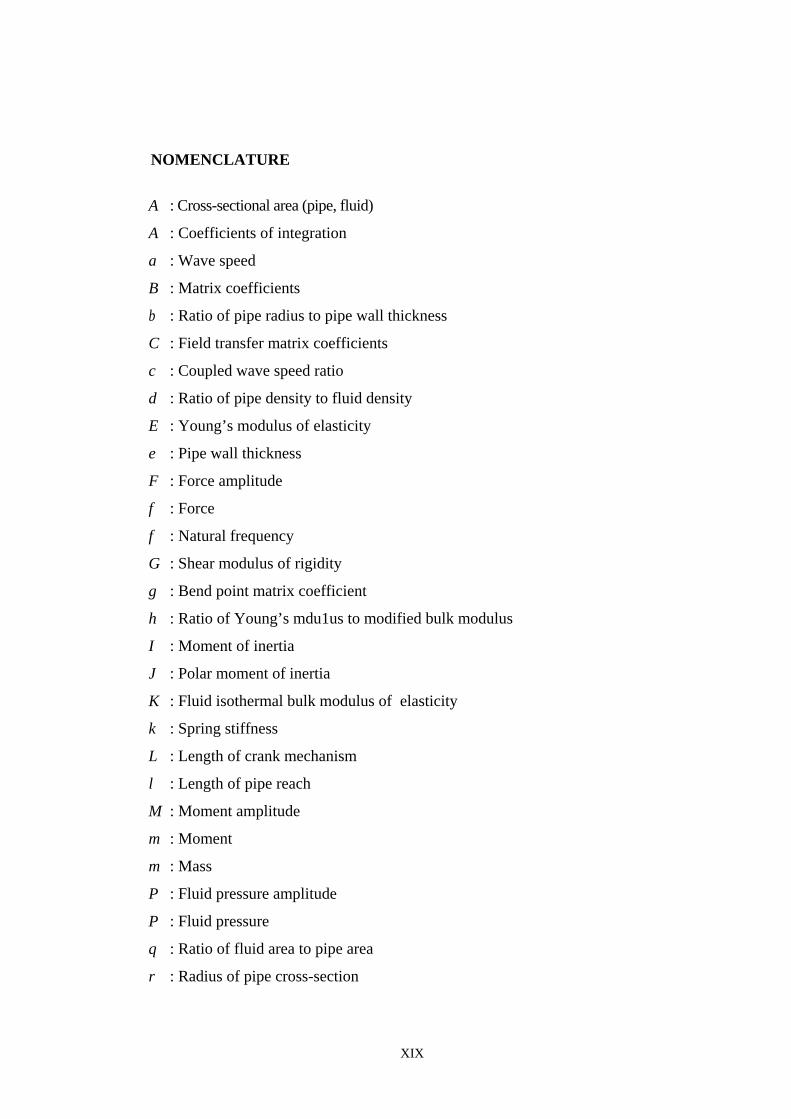
NOMENCLATURE
A : Cross-sectional area (pipe, fluid)
A : Coefficients of integration
a : Wave speed
B : Matrix coefficients
b : Ratio of pipe radius to pipe wall thickness
C : Field transfer matrix coefficients
c : Coupled wave speed ratio
d : Ratio of pipe density to fluid density
E : Young’s modulus of elasticity
e : Pipe wall thickness
F : Force amplitude
f : Force
f : Natural frequency
G : Shear modulus of rigidity
g : Bend point matrix coefficient
h : Ratio of Young’s mdu1us to modified bulk modulus
I : Moment of inertia
J : Polar moment of inertia
K : Fluid isothermal bulk modulus of elasticity
k : Spring stiffness
L : Length of crank mechanism
l : Length of pipe reach
M : Moment amplitude
m : Moment
m : Mass
P : Fluid pressure amplitude
P : Fluid pressure
q : Ratio of fluid area to pipe area
r : Radius of pipe cross-section

XX
s : Coordinate along pipe axis
T : Torque
t : Time
U : Pipe displacement amplitude
u : Pipe displacement
V : Fluid displacement amplitude
v : Fluid displacement
w : Radial displacement
z : Axial displacement
α : Angle between incident pipe reaches
β : Angle of rotation due to shear
Δ : Field transfer matrix coefficient
Δ : Matrix determinant
δ : Differential element
θ : Angular direction
κ : Shape factor for shear
λ : Eigenvalues
υ : Poisson’s ratio
ρ : Mass density
σ : Stress
φ : Angle between local and global axes
Ω : Forcing frequency
ω : Natural circular frequency Γ : Distributed foundation stiffness
τ ,σ ,γ : Field transfer matrix coefficient
Φ : Foundation Modulus

XXI
Subscripts
f : Fluid
G : Global coordinate system
i : Pipe end
L : Local coordinate system
p : Pipe
p : Local axis index
q : Global axis index
R : Rows
s : Spring
t : Time
z : Direction along pipe axis
fp : Fluid and axial pipe wall field transfer matrix
tz : Torsion vibration about z-axis field transfer matrix
xz : Transverse vibration in X-Z plane field transfer matrix
θ : Angular direction
X,Y,Z :Global rectangular coordinate directions
x,y,z :Local rectangular coordinate directions
Superscripts
B : Point matrix for a bend
L : Left of discontinuity
M : Point matrix for a lumped mass
R : Right of discontinuity
S : Point matrix for a spring
T : Matrix transposition
-1 : Matrix inverse

1. INTRODUCTION Ahmet ÖZBAY
1
1. INTRODUCTION
Liquid-filled piping systems are very important for many industrial
applications. They are used for conveying gases and fluids over a wide range of
temperatures and pressures. The failure of piping systems in power or chemical
plants can cause severe economic losses and even loss of human lives. Some of the
design or operation factors that may cause failures in piping systems are: incorrect
support, transient pressure changes, thermal stresses, and flow induced vibration.
In general, a complete dynamic analysis of liquid-filled piping must consider
both the forces of liquid on the piping and the opposing forces of the piping on the
fluid, whether the source of excitation acts on the fluid or the pipe (Budny-1988). For
example, when a hydraulic transient is produced by a sudden valve operation a
pressure pulse is generated in the fluid and this pulse causes structural pipe vibration.
The study of liquid-filled pipes becomes more complicated when several
factors are taken into account. The five families of waves, tees and bends, supports of
various stiffness, structural restraints and hydraulic devices such as pumps, orifices
and valves must be considered. The speed of the wave components depends on pipe
material and fluid properties (Lesmez-1989). The frequencies at which the liquid and
pipe are vibrating are influenced by the structural support configurations of the pipe
and the hydraulic elements of the system.
In this study, the free vibration behavior of air/water-filled piping systems is
first studied with the help of the transfer matrix method (TMM). The existing
governing equations in analytical form which consider the axial, transverse and
torsional vibration of such piping systems are handled in the analysis. Some basic
configurations of copper/steel piping systems such as single span, L-bend, Z-bend, U-
bend and 3-D bend are studied for both fixed-fixed and fixed-free boundary conditions.
ANSYS software program and some experiments completed in this work are used to verify
the present theoretical results together with the results available in the literature. The effect
of the elastic foundation on the natural frequencies is also investigated. A parametric study
is, finally, carried out to understand correctly the vibrational behavior of such piping
systems.
ITD
Highlight
ITD
Highlight
ITD
Highlight

2. LITERATURE REVIEW Ahmet ÖZBAY
2
2. LITERATURE REVIEW
2.1. Flow Induced Vibrations in Pipelines
Flow-induced vibration phenomena have been treated by a variety of
engineering disciplines, each having its particular terminology. In an attempt to
provide a unified overview, let’s propose the following definition of basic elements
of flow-induced vibration:
a) Body oscillators;
b) Fluid oscillators; and
c) Source of excitation.
Oscillators are defied herein as systems of structural or fluid mass that acted
upon by restoring forces if deflected from their equilibrium positions and undergo
vibrations in conjunction with appropriate types of excitation. An engineering system
will usually possess several potential oscillators and several sources of excitation.
The first and most important task in the assessment of possible flow-induced
vibrations is therefore to identify them.
A body oscillator consist of either a rigid structure or part that is elastically
supported so that it can perform linear or angular movements or a structure or
structural part that is elastic in itself so that it can perform flexural movements.
A fluid oscillator consists of a passive mass of fluid that can undergo
oscillations usually governed either by fluid compressibility or by gravity. In both
cases, the oscillating fluid mass can be discrete or it can be distributed. Fluid-flow
systems may contain a number of oscillators. They may give rise to undesirable fluid
pulsations when excited; and they may amplify the vibration of a body oscillator if
one their natural frequencies coincides with the natural body-oscillator frequency.
Sources of excitation for either body or fluid oscillators are numerous and may be
difficult to detect. It is therefore useful to treat them within a basic framework.
• Extraneously induced excitation
• Instability-induced excitation
• Movement-induced excitation
ITD
Highlight
ITD
Highlight
ITD
Highlight
ITD
Highlight
ITD
Highlight
ITD
Highlight
ITD
Highlight
ITD
Highlight
ITD
Highlight

2. LITERATURE REVIEW Ahmet ÖZBAY
3
Extraneously induced excitation is caused by fluctuations in flow velocities or
pressures that are independent of any flow instability originating from the structure
considered and independent of structural movements except for added-mass and
fluid-damping effects.
Movement-induced excitation is due to fluctuating forces that arise from
movements of the vibrating body or fluid oscillator. Vibrations of the latter are thus
self-excited.
The fluid-structure interaction (FSI) in liquid-filled pipe systems has been
investigated extensively, because of its relevance to mechanical, civil, nuclear and
aeronautical engineering.
By using Bernoulli-Euler beam theory, Wilkinson (1978) showed that under
certain conditions the vibrations of the liquid column and that of the supporting
structure can interact.
Chaudhry (1979) and Wylie and Streeter (1982) give transfer matrices
corresponding to almost every element in hydraulic piping systems such as
oscillating valve, fixed orifice, pump, pipe bend accumulators, and uncoupled
straight pipe elements.
Otwell (1984) developed and verified a numerical model with experimental
data. The one-dimensional equations of continuity and momentum for the liquid and
pipe wall were solved by the method of characteristics. At an elbow, coupling was
introduced by continuity relationships. The translation of attached piping at an elbow
was represented by an added stiffness term, and solved simultaneously with the
characteristic equations. The equations were normalized and dimensionless
parameters were identified that describe the liquid-pipe interaction.
Budny (1988) evaluated the four equation model concerned with only axial
wave propagation and Poisson coupling to account for the fluid-structure interaction.
The developed model includes viscous damping and a fluid shear stress term to
account for the structural and liquid energy dissipation. If a piping system is to be
exposed to a steady state pipe vibration, fixing the piping with a rigid support will
limit the pressure rise to its minimum. However, if motion must be permitted, as in
the case of expansion loops, then installing a stiff damper is suggested.
ITD
Highlight
ITD
Highlight
ITD
Highlight
ITD
Highlight

2. LITERATURE REVIEW Ahmet ÖZBAY
4
Wiggert et al. (1987) extended Wilkinson’s work by including the Poisson’s
effect and by using the Timoshenko beam theory. Experimental results with an L-
shaped pipe showed a good agreement with the numerical model.
Lesmez used the same model with a U-shaped bend for a variable length
piping system.
Baasri (1990) investigated the phenomenon of air release during hydraulic
transients in pipe flow with column separation. It was established that when line
pressure during a hydraulic transient drops to the vapor pressure of the liquid column
separation and cavitations bubbles occur throughout the system, and that air release
from saturated water is initiated towards these bubbles by the process of convective
diffusion. At the time of cavity collapse, the sudden increase in pressure causes the
system to agitate. This agitation significantly increases the rate of air release and
with disappearance of all vapor cavities small gas bubbles scattered throughout the
system are left behind. These gas bubbles cause a considerable decrease in both the
wave speed of the medium and the peak pressures.
Yakut (1996) investigated the flow acoustic coupling phenomenon
experimentally. Yakut (1996) observed from experiments that the flow-acoustic
coupling was realized if vortex-shedding frequency locked on the natural acoustic
frequency and its harmonics of pipeline.
Tusseling (1996) reviewed the literature on transient phenomena in liquid-
filled pipe systems up to 1996.
Li (1997) has studied; a specially designed multi-span tube array test rig was
used to investigate the effects of partial flow admission. Using this test rig the water
flow can pass across any location along the tube span. Various end supports were
used in the different experimental setups. Therefore, not only the first mode but also
the higher vibration modes can be excited, depending on the location of the flow and
tube-support configurations. It was been found that vibration modes higher than the
third mode do not have significant vibration displacement. The experiments show
that the fluid energy is additive along the span, regardless of the tube mode shape.
Response peaks were observed prior to the ultimate fluid-elastic instability. By
analyzing the corresponding Strouhal numbers, it was found that both vortex
2. LITERATURE REVIEW Ahmet ÖZBAY
5
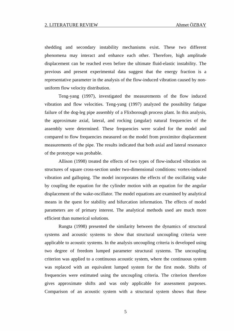
shedding and secondary instability mechanisms exist. These two different
phenomena may interact and enhance each other. Therefore, high amplitude
displacement can be reached even before the ultimate fluid-elastic instability. The
previous and present experimental data suggest that the energy fraction is a
representative parameter in the analysis of the flow-induced vibration caused by non-
uniform flow velocity distribution.
Teng-yang (1997), investigated the measurements of the flow induced
vibration and flow velocities. Teng-yang (1997) analyzed the possibility fatigue
failure of the dog-leg pipe assembly of a Flixborough process plant. In this analysis,
the approximate axial, lateral, and rocking (angular) natural frequencies of the
assembly were determined. These frequencies were scaled for the model and
compared to flow frequencies measured on the model from proximitor displacement
measurements of the pipe. The results indicated that both axial and lateral resonance
of the prototype was probable.
Allison (1998) treated the effects of two types of flow-induced vibration on
structures of square cross-section under two-dimensional conditions: vortex-induced
vibration and galloping. The model incorporates the effects of the oscillating wake
by coupling the equation for the cylinder motion with an equation for the angular
displacement of the wake-oscillator. The model equations are examined by analytical
means in the quest for stability and bifurcation information. The effects of model
parameters are of primary interest. The analytical methods used are much more
efficient than numerical solutions.
Rungta (1998) presented the similarity between the dynamics of structural
systems and acoustic systems to show that structural uncoupling criteria were
applicable to acoustic systems. In the analysis uncoupling criteria is developed using
two degree of freedom lumped parameter structural systems. The uncoupling
criterion was applied to a continuous acoustic system, where the continuous system
was replaced with an equivalent lumped system for the first mode. Shifts of
frequencies were estimated using the uncoupling criteria. The criterion therefore
gives approximate shifts and was only applicable for assessment purposes.
Comparison of an acoustic system with a structural system shows that these

2. LITERATURE REVIEW Ahmet ÖZBAY
6
equilibrium equations in these two systems were exactly the same. Therefore, the
uncoupling criteria developed for structural systems are applicable for acoustic
systems.
Gidi’s (1999) investigations have focused on flow regime and two-phase flow
damping ratio. However, tube bundles in steam generators have vapor generated on
the surface of the tubes, which might affect the flow regime, void fraction
distribution, turbulence levels and tube-flow interaction, al1 of which have the
potential to change the tube vibration response. In Gidi’s (1999) study, flows regime
for bundle void generation was at al1 times bubbly and homogeneous, while the
upstream void friction generation cases showed a clear tendency to chum flow. A
change in flow regime from bubbly to chum flow will produce the same effect as an
increase in turbulence buffeting levels, and hence it seems difficult with the present
knowledge to distinguish between the two causes. In as much as turbulence levels are
related to flow regime, it is essential to have a clear knowledge of the flow regime in
steam generators in order to predict the fluid-elastic instability threshold of the tubes.
Evgin (2000) evaluated the effects of interface strength on the behavior of
buried flexible pipe.
Kartha (2000) studied experimentally explores the potential of different
active, passive and active/passive control methodologies for control of vibrational
power flow in fluid filled pipes. Circumferential modal decomposition and
measurements of vibrational power carried by individual wave types were carried out
experimentally. The importance of dominant structural bending waves and the need
to eliminate them in order to obtain meaningful experimental results has been
demonstrated. The effectiveness of the rubber isolator in reducing structural waves
has been demonstrated. Improved performance of the quarter wavelength tube and
Helmholtz resonator was obtained on implementation of the rubber isolator on the
experimental rig. Active control experiments using the side-branch actuator and 1/3
piezoelectric composite yielded significant dB reductions revealing their potential for
practical applications. A combined active/passive approach was also implemented as
part of this work. This approach yielded promising results, which proved that

2. LITERATURE REVIEW Ahmet ÖZBAY
7
combining advantages of both active and passive approaches was a feasible
alternative.
Durrani (2001) treated the dynamics of pipelines with a finite element
method. In his thesis a Finite Element Method (FEM) has developed for the
application of Coriolis force on a fluid filled Pipeline. He has calculated the
deflections and mode shape frequencies with the selected project data first using
standard textbook methods, second using the industrial methods and third using one
of the commercial software ANSYS. Nine cases were studied using this FEM and
actual industrial project data. The resultant data shows noticeable effects of Coriolis
force at relatively higher flow velocities.
Taking into account all the three major coupling mechanism, namely the
friction coupling, Poisson coupling and junction coupling, Li et al. (2002) studied the
vibration analysis of a liquid-filled pipe system by the transfer matrix method.
Evans (2004) presents a theory and experimental research relating the mass
flow rate within a pipe to pipe vibration. This approach has the potential to develop
into a non-intrusive, low-cost, flow rate measurement. Experimental results indicate
a nearly quadratic relationship between the signal noise and mass flow rate in the
pipe. This relationship is believed to be caused by friction coupling between the fluid
and the pipe. It is also shown that the signal noise-mass flow rate relationship is also
dependent on the pipe material and pipe diameter.
Nieves (2004) investigated the flow-induced vibration. Three finite elements
models for the pipe system were developed: a structural finite element analysis
model with multi support system for frequency analysis, a fluid structure interaction
(FSI) finite element model and a transient flow model for water hammer induced
vibration analysis in a fluid filled pipe. The natural frequencies, static, dynamic and
thermal stresses, and the limitation of the pipeline system were investigated. The
investigation demonstrates that a gap in a support at the segment k has a negative
effect on the entire piping system. In the water-hammer analysis, the limit maximum
flow rates were determined based on the rate of a rapid closure of the isolation valve.
A study of the fluid transient in a simple pipeline was performed. Results obtained
from FE model for fluid-structure interaction was compared with a model without
ITD
Highlight

2. LITERATURE REVIEW Ahmet ÖZBAY
8
considering fluid-structure interaction effects. The results show notable differences
in the velocities profile and deformation due to the fluid-structure interaction effects.
2.2. Transfer Matrix Method
Lesmez (1989) formulated the vibration of liquid-filled piping system by
using one-dimensional wave theory in both the liquid reaches and the pipe wall.
Considering both the junction coupling and Poisson coupling, he used the transfer
matrix method to study the motion of these systems
Akdoğan (1992) studied the transfer matrix method implemented to carry
dynamic analysis of piping systems with the Euler-Bernoulli beam theory. The
analysis involves determination of dynamic characteristics and steady state harmonic
response for such systems, especially at low frequencies. In his work the junction
coupling and Poisson coupling are considered.
Servaites (1996) analyzed the static and dynamic behavior of steel smoke
stacks subject to excitation by aerodynamic forces. A computer program created
modifying an existing analysis code, to be used specifically for stack analysis. This
analysis code utilizes the transfer matrix method to perform detailed bending and
vibration analyses. A detailed analysis was performed to demonstrate the validity of
approximating a tapered Timoshenko beam with a series of continuous, constant
cross-section beams.
Dolasa (1998) developed a design tool to analyze and design un-damped
beam and rotor systems in two dimensions. Systems modeled in two dimensions,
such as beams with different moments of inertia, could produce varying responses in
the each direction of motion. A coupling between the vertical and horizontal motions
also exists in rotor systems mounted of fluid film bearings. The transfer matrix
method has been used in the development of the software and an explanation of the
method is included in his thesis.
Fang Yu (2001) developed a method for exact vibration analysis of 3-D frame
structures. The transfer matrix for each beam element was rearranged in dynamic
stiffness matrix that was called dynamic stiffness matrix that related beam end forces
ITD
Highlight
ITD
Highlight
ITD
Highlight

2. LITERATURE REVIEW Ahmet ÖZBAY
9
and displacements. For each frequency, an eigenvector for displacement at the ends
of beam elements could be computed and the associated eigen function could be
determined by the eigenvector and the dynamic shape function based on the Euler-
Bernoulli and Timoshenko beam theories. Several examples were presented to
demonstrate the principles and algorithms and the results were compared and show
good agreement with those computed ANSYS or given in the references.
Daneshfaraz and Kaya (2007) presented an approach for the application of the
method of transfer matrix to the analysis of one dimensional flow problems hydraulic
branch of civil engineering, and to the lateral dynamic analysis of multi-storey
buildings. At their study various examples taken from the literature solved using
transfer matrix method. It was seen that the transfer matrix approach was in
sufficient agreement with other methods.

3. MATERIAL AND METHOD Ahmet ÖZBAY
10
3. MATERIALS AND METHOD
3.1. Material
The aim of the experiments is to support the theoretical solutions obtained
with the help of the transfer matrix method.
In order to measure the liquid natural frequencies; 4 tanks, valves and 2
pressure transducers were used. Two tanks were used as upstream tanks, the other
two were used as downstream tanks. The tanks were pressurized with the air that had
a maximum pressure of 4 Bar. Figure.3.1. shows the general piping setup used in this
study.
Figure 3.1. Pipeline Test-Rig
If the length of the pipe is known, the fundamental frequency and harmonics
are determined. An open-closed system results closure of the valve and excites the
ITD
Highlight
ITD
Highlight
ITD
Highlight

3. MATERIAL AND METHOD Ahmet ÖZBAY
11
odd harmonics of the liquid. The fundamental frequency of an open-closed liquid
system is given by
lc
f ff 4= (3.1)
where ff is the fundamental frequency of the liquid, l is the length of the pipe, and cf
is the coupled wave speed which will described in Equations (3.22) and (3.23).
In order to measure the first structural natural frequency of the pipe
configurations, impact hammer test was applied. In this method, structure is excited
by hammer and causes it to vibrate while the structure is monitoring with
accelerometers and FFT analyzer. It gives significant peaks at its natural frequencies
in FFT spectrums. This method is tested by different samples before used in
experiments and proved its appropriateness. Also this method was used by Çınar
(1998) to define the natural frequencies of the piping system.
3.1.1. Pipe Materials
One inch nominal diameter cooper pipe and two inch nominal diameter steel
pipe types were used in the experiments. Table 3.1. and Table 3.2. list the physical
properties of the piping system.
Table 3.1. Physical properties of copper pipe
Young’s Modulus ( E ) 97 GPa
Density ( ρ ) 8350 kg/m3
Inside Radius ( r ) 14 mm
Thickness ( e ) 1 mm
Poisson’s Ratio (υ ) 0.35
ITD
Highlight
ITD
Highlight
ITD
Highlight
ITD
Highlight

3. MATERIAL AND METHOD Ahmet ÖZBAY
12
Table 3.2. Physical properties of steel pipe
Young’s Modulus ( E ) 157 GPa
Density ( ρ ) 7600 kg/m3
Inside Radius ( r ) 28.15 mm
Thickness ( e ) 3.6 mm
Poisson’s Ratio (υ ) 0.28
3.1.2. Liquid
The liquid that is used in the experiments is from the Soda Ash Plant water
supply system. Table 3.3. lists the physical properties of the water.
Table 3.3. Physical properties of liquid
Temperature 25.0 °C
Bulk Modulus ( K ) 2.2 GPa
Density ( ρ ) 997.0 kg/m3
3.1.3. External Shaker
The pipe was excited by an external shaker, which produces reciprocating
force. The shaker is a crank-slider mechanism that transfers rotary motion to
reciprocating motion. The shaker consists of a motor, pulley, crank and connecting
rod.
ITD
Highlight
ITD
Highlight
ITD
Highlight
ITD
Highlight

3. MATERIAL AND METHOD Ahmet ÖZBAY
13
Figure 3.2. Crank mechanism
Gamak Type AGM 3-phase cage induction motor with Altivar 58
Telemechanic variable speed controller was used in experiments. The speed was
increased by the pulley form 2840 rpm to 6090 rpm.
3.1.4. Transducers
Two pressure transducers and one portable vibration data collector were used
for pressure and vibration measurements.
Fuji electric gauge pressure transmitter model FKG was used for recording
the pressure.
The DLI Watchman® DCA-20 Portable Data Collector was used a single-
channel FFT analyzer and DLI Engineering’s ExpertALERT™ vibration analysis
software was used in experiments.

3. MATERIAL AND METHOD Ahmet ÖZBAY
14
Figure 3.3. Fuji electric gauge pressure transmitter model FKG
Figure 3.4. The DLI Watchman® DCA-20 portable data collector

3. MATERIAL AND METHOD Ahmet ÖZBAY
15
3.2. Method
3.2.1. Governing Equations
In this section differential equations available in the literature which govern
the free vibration behavior of liquid-filled piping systems are presented as in the
same in Lesmez ‘s study (1989).
Figure 3.5. shows a general pipe reach with the sign convention used in this
study. The z-axis is considered coincident with the centerline of the pipe reach.
zzf
f'f yyy δ
∂
∂+=
Figure 3.5. Sign convention for internal forces (Lesmez,1989)
3.2.1.1. Axial Vibration – Liquid and Pipe Wall
The fluid is assumed to be one-dimensional (the radial component of the fluid
velocity is zero and the flow is developed in only the radial direction), linear, and
X
Z
Y
v
f’x
fz
f’z
fy
fx
f’y
mz
mx my
m’z
m’x
m’y
δz
re
ITD
Highlight
ITD
Highlight
ITD
Highlight
ITD
Highlight
ITD
Highlight
ITD
Highlight
ITD
Highlight
ITD
Highlight

3. MATERIAL AND METHOD Ahmet ÖZBAY
16
homogeneous, with isotropic flow and uniform pressure and fluid velocity over the
cross-section. The pipe wall is assumed to be linearly elastic, isotropic, prismatic,
circular and thin-walled.
Two equations represent the axial continuity and momentum relations for the
liquid:
02 2
=⎥⎦
⎤⎢⎣
⎡∂∂
∂+
∂∂
+∂∂
ztv
tw
rK
tp (3.2)
02 02
2
=+∂∂
+∂∂
rtv
zp
fτρ (3.3.a)
in which p = p(z,t) is the fluid pressure, v = v(z,t) is the fluid displacement, and
w = w(z,t) is the pipe wall displacement. K and ρf are the fluid bulk modulus and
density, r is the inside radius of the pipe, and the shear stress along the pipe wall is
represented by τ0. In these equations it is assumed that the fluid density is constant
(the convective terms are ignored by assuming low Mach numbers, where the fluid
wave speed is much greater than the fluid velocity) and the radial component of the
fluid velocity is zero. The fluid friction term in the momentum equation can be
neglected for forced vibrations.
02
2
=∂∂
+∂∂
tv
zp
fρ (3.3.b)
Assuming an axisymmetric, linear elastic pipe walls with small deformations
and no buckling, the axial and circumferential stress-strain relationships for the pipe-
wall are
0* =⎥⎦⎤
⎢⎣⎡ +∂∂
−rw
zuE z
z υσ (3.4)
ITD
Highlight
ITD
Highlight
ITD
Highlight
ITD
Highlight
ITD
Rectangle
ITD
Highlight
ITD
Highlight
ITD
Highlight
ITD
Highlight
ITD
Highlight
ITD
Highlight
ITD
Highlight
ITD
Highlight

3. MATERIAL AND METHOD Ahmet ÖZBAY
17
0* =⎥⎦⎤
⎢⎣⎡
∂∂
+−zu
rwE zυσθ (3.5.a)
where the modified modulus of elasticity is defined as
( )2*
1 υ−=
EE (3.5.b)
in which σz = σz (z,t) and σθ = σθ (z,t) are the stresses in the axial and radial direction,
uz = uz (z,t) is the pipe wall displacement in the axial direction, and E and υ are the
Young's modulus and Poisson's ratio of the pipe wall, respectively. Figures 3.6 and
3.7 show a section of a pipe with stresses and displacements in the axial and radial
directions.
Figure 3.6. Axial pipe element
XY
Z
δz
v
σz
e
uz (axial) w (radial)
σz+ z
z
∂∂σ δz
ITD
Rectangle
3. MATERIAL AND METHOD Ahmet ÖZBAY
18
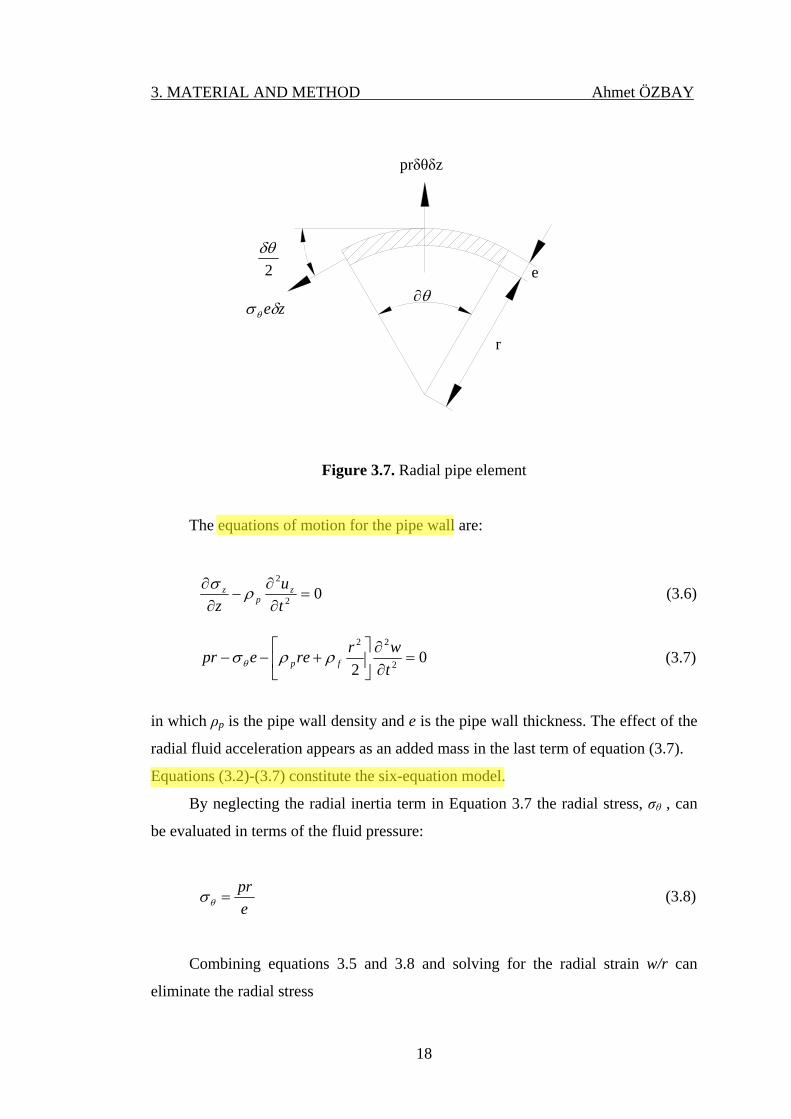
Figure 3.7. Radial pipe element
The equations of motion for the pipe wall are:
02
2
=∂∂
−∂∂
tu
zz
pz ρσ (3.6)
02 2
22
=∂∂
⎥⎦
⎤⎢⎣
⎡+−−
twrreepr fp ρρσθ (3.7)
in which ρp is the pipe wall density and e is the pipe wall thickness. The effect of the
radial fluid acceleration appears as an added mass in the last term of equation (3.7).
Equations (3.2)-(3.7) constitute the six-equation model.
By neglecting the radial inertia term in Equation 3.7 the radial stress, σθ , can
be evaluated in terms of the fluid pressure:
epr
=θσ (3.8)
Combining equations 3.5 and 3.8 and solving for the radial strain w/r can
eliminate the radial stress
zeδσθ
2δθ
θ∂ e
prδθδz
r
ITD
Highlight
ITD
Highlight
ITD
Rectangle
3. MATERIAL AND METHOD Ahmet ÖZBAY
19
zu
eEpr
rw z
∂∂
−= υ* (3.9)
Combining equations 3.4 and 3.9 give the expression for the axial stress
0=∂∂
−−zuEp
er z
z υσ (3.10.a)
multiply the above equation by the pipe cross-section area Ap, to obtain the axial
force, fz
0=∂∂
−−z
zppz
uEAperAf υ (3.10.b)
Differentiating Equation 3.9 with respect to time and combining it with
Equation 3.2 produces the expression for the fluid pressure
022
*2
* =∂∂
∂+
∂∂∂
−∂∂
ztvK
ztuK
zp zυ (3.11.a)
where
eErK
KK*
*
21+= (3.11.b)
Equations 3.3b, 3.6, 3.10.b and 3.11 constitute the four-equation model
presented by Otwell (1984), and Budny (1988). Differentiating Equations 3.3b and
3.6 with respect to the axial direction z, then differentiating Equations 3.10b and 3.11
with respect to time and combining them to solve for the axial force and fluid
pressure, can further reduce the followings.
ITD
Rectangle

3. MATERIAL AND METHOD Ahmet ÖZBAY
20
02
2
2
2
2
22 =
∂∂
+∂∂
−∂∂
tpbA
tf
zfa p
zzp υ (3.12)
02
2
22
2
2
2
22 =
∂∂
+∂∂
−∂∂
zf
dAa
tp
zpa z
p
ff
υ (3.13.a)
where
ff
Kaρ
*2 = (3.13.b)
pp
Eaρ
=2 (3.13.c)
erb = (3.13.d)
f
pdρρ
= (3.13.e)
In Equations 3.13.b and 3.13.c, af and ap are the non-coupled fluid and axial
pipe wall wave speeds, respectively, b is the pipe radius to wall thickness ratio and d
is the density ratio. Equations 3.12 and 3.13.a are second order partial differential
equations in the fluid pressure and axial pipe wall force. They may be expressed in
matrix form as:
010
12
0
2
2
2
2
22
2
=⎭⎬⎫
⎩⎨⎧
∂⎥⎦
⎤⎢⎣
⎡ −−
⎭⎬⎫
⎩⎨⎧
∂∂
⎥⎥⎥
⎦
⎤
⎢⎢⎢
⎣
⎡
pf
tdbA
pf
zaadA
azpz
ffp
p υυ (3.14a)
A similar equation can be obtained for the axial pipe wall and fluid
displacements by combining and solving Equations 3.3.b, 3.6, 3.10.b and 3.11.a.
ITD
Rectangle
ITD
Highlight
ITD
Highlight
ITD
Rectangle
ITD
Rectangle

3. MATERIAL AND METHOD Ahmet ÖZBAY
21
02
001
2
22
2
2
2
22
2222
=⎭⎬⎫
⎩⎨⎧
∂⎥⎥⎦
⎤
⎢⎢⎣
⎡−
⎭⎬⎫
⎩⎨⎧
∂∂
⎥⎥⎥
⎦
⎤
⎢⎢⎢
⎣
⎡
−
−+
vu
td
db
vu
zadba
db
adbaa
db
zz
ff
fpf
υ
υυ (3.14b)
Poisson terms couple equation 3.12 and 3.13.a as shown by the off-diagonal
elements of the matrices in Equations 3.14.a and 3.14.b.
The separation of variables technique is used to solve for the force fz and fluid
pressure p in Equation 3.14a. Three steps are necessary to solve for the dependent
variables in the above equation: i) convert the partial differential equation into
ordinary differential equation, ii) find solutions for the ordinary differential equation,
and iii) find the constants of integration of the differential equation. The solution for
the constants of integration will be postponed to the next chapter since they depend
on the boundary conditions imposed on the piping system.
i) Separation of Variables
Assuming a harmonic oscillation for the time dependence, which is
appropriate for oscillatory flow and oscillatory structural motion in the axial
direction, we can write:
jwt
zz ezFtzf )(),( = (3.15)
jwt
zz ezptzp )(),( = (3.16)
where F(z) and P(z) are functions of z only, ω is the oscillatory frequency and
1−=j
Substituting the above equations into Equation 3.14 yields the ordinary
differential equation in Fz and P.
ITD
Highlight
ITD
Highlight
ITD
Highlight
ITD
Highlight
ITD
Highlight
ITD
Highlight
ITD
Highlight
ITD
Highlight
ITD
Rectangle
ITD
Rectangle
3. MATERIAL AND METHOD Ahmet ÖZBAY
22
010
12
02
22
2
=⎭⎬⎫
⎩⎨⎧⎥⎦
⎤⎢⎣
⎡ −+
⎭⎬⎫
⎩⎨⎧
⎥⎥⎥
⎦
⎤
⎢⎢⎢
⎣
⎡
PFbA
PF
aadA
azp
ıı
ıı
ffp
p υωυ (3.17)
where Fzıı and Pıı are the derivatives with respect to the axial direction z. The
elimination method can be used to reduce Equation 3.17 to a single dependent
variable. This procedure yields
0)(24 =+
+++
lF
lF ıııv τσγστ (3.18.a)
where l is the length of a pipe reach and
2
22
falωτ = (3.18.b)
2
22
palωσ = (3.18.c)
2
2222
pdalbωυγ = (3.18.d)
Equation 3.18.a is a fourth-order, ordinary differential equation with constant
coefficients.
ii) Solution of the Ordinary Differential Equation
The solutions for Fz in Equation 3.18a is of the form
lz
z eAzFλ
=)( (3.19)
ITD
Highlight

3. MATERIAL AND METHOD Ahmet ÖZBAY
23
where A is a constant.
Substitution of Equation 3.18 into 3.17.a produces the characteristic equation
in λ:
0)( 24 =++++ στλγστλ (3.20)
where λ is the characteristic value. The roots of this equation are ±jλ1 and ±jλ2 ,
where
στγστγστλ 421 2
212 −++±++= )()(, (3.21)
This equation can also be expressed as:
⎪⎭
⎪⎬⎫
⎪⎩
⎪⎨⎧
−⎥⎦⎤
⎢⎣⎡ ++−⎥⎦
⎤⎢⎣⎡ ++== 22
222222222
21
222 422
21
pffpffpff aaadbaaa
dbaalc υυ
λω (3.22)
⎪⎭
⎪⎬⎫
⎪⎩
⎪⎨⎧
−⎥⎦⎤
⎢⎣⎡ +++⎥⎦
⎤⎢⎣⎡ ++== 22
222222222
22
222 422
21
pffpffpfp aaadbaaa
dbaalc υυ
λω (3.23)
The above equations give the expressions for the coupled wave speeds. These
coupled speeds are the same as those derived by Budny (1988) and Lesmez (1989) using
the method of characteristics. An inspection of Equations 3.22 and 3.22, assuming
no coupling between liquid and pipe wall by neglecting the second order Poisson terms,
yields
22
1fawl
=⎟⎟⎠
⎞⎜⎜⎝
⎛λ
(3.24.a)
ITD
Highlight
ITD
Rectangle
ITD
Highlight
ITD
Highlight
ITD
Rectangle
ITD
Rectangle

3. MATERIAL AND METHOD Ahmet ÖZBAY
24
22
2pawl
=⎟⎟⎠
⎞⎜⎜⎝
⎛λ
(3.24.b)
Placing Equation 3.21 into 3.19, the solution for Fz (z) is:
lzj
lzj
lzj
lzj
z eAeAeAeAzF 2211
4321)(λλλλ −−−
+++= (3.25)
and using the relation
)lzsin(j)
lzcos(e
)lz(j
λλλ
±=±
(3.26)
Equation 3.24 can be written in the following form
)lzsin(A)
lzcos(A)
lzsin(A)
lzcos(A)z(Fz 24231211 λλλλ +++= (3.27.a)
where
211 AAA += (3.27.b) )( 212 AAjA −= (3.27.c) 433 AAA += (3.27.d) )( 434 AAjA −= (3.27.e)
iii) Solution for the Constants of Integration
The solutions for the pipe wall and fluid displacements and the fluid pressure
are of the same form as Equation 3.27a. To solve for the four dependent variables,
the constants of integration A1, A2, A3 and A4 must have known values. Expressing the
ITD
Highlight
ITD
Rectangle
ITD
Rectangle

3. MATERIAL AND METHOD Ahmet ÖZBAY
25
axial and fluid displacements in similar forms as the force and fluid pressure in Equations
3.15 and 3.16 gives
jwt
zz ezUtzu )(),( = (3.28)
jwtzz ezVtzv )(),( = (3.29)
Placing Equation 3.28 into 3.6 and combining with Equation 3.27.a we obtain
the solution for the axial displacement:
⎭⎬⎫
⎩⎨⎧
⎥⎦⎤
⎢⎣⎡ −+⎥⎦
⎤⎢⎣⎡ −= )
lzcos(A)
lzsin(A)
lzcos(A)
lzsin(A
EAl)z(U
pz 2423212111 λλλλλλ
σ (3.30)
The fluid pressure is obtained by placing Equations 3.27.a and 3.30 into
3.11.b
( ) ( )⎭⎬⎫
⎩⎨⎧
⎥⎦⎤
⎢⎣⎡ +−+⎥⎦
⎤⎢⎣⎡ +−= )
lzsin(A)
lzcos(A)
lzsin(A)
lzcos(A
bA)z(P
pz 2423
221211
21
1 λλλσλλλσσυ
(3.31)
Finally, the fluid displacement is obtained by placing Equations 3.29 and
3.31 into 3.3b
( ) ( )⎭⎬⎫
⎩⎨⎧
⎥⎦⎤
⎢⎣⎡ −−+⎥⎦
⎤⎢⎣⎡ −−
−= )
lzcos(A)
lzsin(A)
lzcos(A)
lzsin(A
bKAl)z(V *
pz 24232
2212111
21 λλλλσλλλλσ
τσυ
(3.32)
Arranging Equations 3.27.a, 3.28, 3.31 and 3.32 into matrix form we obtain
ITD
Rectangle
ITD
Highlight
ITD
Highlight
3. MATERIAL AND METHOD Ahmet ÖZBAY
26
⎪⎪⎭
⎪⎪⎬
⎫
⎪⎪⎩
⎪⎪⎨
⎧
⎥⎥⎥⎥⎥⎥⎥⎥⎥
⎦
⎤
⎢⎢⎢⎢⎢⎢⎢⎢⎢
⎣
⎡
⎟⎠⎞
⎜⎝⎛
⎟⎠⎞
⎜⎝⎛
⎟⎠⎞
⎜⎝⎛
⎟⎠⎞
⎜⎝⎛
⎟⎠⎞
⎜⎝⎛
⎟⎠⎞
⎜⎝⎛−⎟
⎠⎞
⎜⎝⎛
⎟⎠⎞
⎜⎝⎛−
⎟⎠⎞
⎜⎝⎛
⎟⎠⎞
⎜⎝⎛
⎟⎠⎞
⎜⎝⎛
⎟⎠⎞
⎜⎝⎛
⎟⎠⎞
⎜⎝⎛−⎟
⎠⎞
⎜⎝⎛
⎟⎠⎞
⎜⎝⎛−⎟
⎠⎞
⎜⎝⎛
=
⎪⎪⎭
⎪⎪⎬
⎫
⎪⎪⎩
⎪⎪⎨
⎧
4
3
2
1
2211
26261515
24241313
22221111
AAAA
lzsin
lzcos
lzsin
lzcos
lzcosB
lzsinB
lzcosB
lzsinB
lzsinB
lzcosB
lzsinB
lzcosB
lzcosB
lzsinB
lzcosB
lzsinB
FVP
U
Z
Z
λλλλ
λλλλ
λλλλ
λλλλ
(3.33.a)
where
σλEA
lBp
11 = (3.33.b)
σλEA
lBp
22 = (3.33.c)
υσλσ
bAB
p
21
3−
= (3.33.d)
υσλσ
bAB
p
22
4−
= (3.33.e)
υστλλσ
*1
21
5)(
bKAl
Bp
−= (3.33.f)
υστλλσ
*2
22
6)(
bKAl
Bp
−= (3.33.g)
3.2.1.2. Transverse Vibration in x-z Plane
Consider the free body diagram of an element of a beam bending in the x-z
plane shown in Figures 3.8.and 3.9. Where my is the internal bending moment, φy is
the rotation due to bending deformation, and fx is the internal shear force.
ITD
Highlight
ITD
Rectangle

3. MATERIAL AND METHOD Ahmet ÖZBAY
27
Figure 3.8. Sign convention for pipe element
⎥⎦⎤
⎢⎣⎡ −∂∂
= yϕκz
uGAf x
spx yspGA βκ= (3.34.a)
)1(2 υ+=
EG (3.34.b)
υυκ
34)1(2
++
=s (3.34.c)
where G is the shear modulus, Apκs represents the effective shear area of the section
and κs is the shape factor for a thin-walled tube.
Y
Z
Original
Deformed
X
φy
βy
zux
∂∂

3. MATERIAL AND METHOD Ahmet ÖZBAY
28
Figure 3.9. my and fx forces in x-z plane.
From the elementary beam theory
0=∂∂
−z
EIm Ypy
ϕ (3.35)
where Ip is the moment of inertia about the y-axis for the pipe wall. From equilibrium
conditions Figure 3.9.
02
2
=∂∂
−∂∂
tu
zf xx μ (3.36)
02
2
=∂
∂−+
∂
∂
tf
m yx
z
y ϕφ (3.37)
Y
Z
X
φy
my
fx
zz
xx
ff δ
∂∂
+
zz
yy
mm δ
∂
∂+
zδ

3. MATERIAL AND METHOD Ahmet ÖZBAY
29
where
ffpp AA ρρμ += (3.38)
ffpp II ρρφ += (3.39)
and If is the moment of inertia about the y-axis for the fluid. Solving for φy and ux in
Equations (3.34.a) and (3.36), substituting the results in Equation (3.35) and
eliminating my from Equation (3.38), we obtain a fourth-order partial differential
equation in fx(z,t):
02
2
2
2
2
2
2
2
22
4
2
2
4
4
=⎥⎦
⎤⎢⎣
⎡∂∂
∂∂
+⎥⎦
⎤⎢⎣
⎡∂∂
∂∂
+∂∂
∂−
∂∂
+∂∂
tf
tGAtf
zGAEI
tzf
tf
zf
EI x
sp
x
sp
pxxxp μ
κμμ
κφμ
(3.40)
By neglecting rotatory inertia and shear deformation terms in equation 3.40,
we obtain the Euler- Bernoulli beam equation in the shear force fx,
02
2
4
4
=∂∂
+∂∂
tf
zf
EI xxp μ (3.41)
The separation of variables technique is used to solve for the dependent
variable fx, in time, t, and axial direction z.
tj
xx ezFtzf ω)(),( = (3.42)
Substitution of the above equation into Equation (3.39) we obtain
042 =⎥⎦⎤
⎢⎣⎡ −
−+
+ xıı
xiv
x Fl
Fl
F στγτσ (3.43)
ITD
Highlight
ITD
Highlight
ITD
Rectangle
ITD
Highlight
ITD
Rectangle
ITD
Rectangle
ITD
Highlight
ITD
Rectangle
ITD
Note
for the case of nonlinear transverse vibration equation single frequency input --> multiple frequency output we use Excitaion pulsating flow ( single frequency input) u(t)=u0+u1 e^(i w t) p(t)=p0 + p1 e^(i w t) and the solution (multiple frequency output) f(z,t) = Fx(z) A(n) e^(i n w t)

3. MATERIAL AND METHOD Ahmet ÖZBAY
30
where
22lGA sp
ωκ
μσ = (3.44.a)
22l
EI p
ωφτ = (3.44.b)
42l
EI p
ωμγ = (3.44.c)
and l is the length of the pipe reach. The solution of a fourth-order ordinary
differential equation with constant coefficient shown in Equation (3.43) is given by
lz
x eA)z(Fλ
= (3.45)
where A is a constant. Substitution of Equation (3.45) into (3.43) produces the
characteristic equation in λ:
0)()( 24 =−+++ στγλστλ (3.46)
The roots of this equation are ±jλ1 and ±jλ2 , where
)(21))(
41(
22
2,12 τστσγλ +
⎭⎬⎫
⎩⎨⎧ −+= m (3.47)
From Equation (3.45) we may write
lzj
lzj
lz
lz
x eAeAeAeA)z(F 2211
4321
λλλλ −−−+++= (3.48)
and using the relations
ITD
Rectangle
ITD
Rectangle
3. MATERIAL AND METHOD Ahmet ÖZBAY
31
)lzsinh()
lzcosh(e
)lz(
λλλ
±=±
and )lzsin(j)
lzcos(e
)lz(j
λλλ
±=±
(3.49)
Equation (3.48) can be written in the following form
)lzsin(A)
lzcos(A)
lzsinh(A)
lzcosh(A)z(Fx 24231211 λλλλ +++= (3.50.a)
where
211 AAA += (3.50.b) 212 AAA −= (3.50.c) 433 AAA += (3.50.d) )( 434 AAjA −= (3.50.e)
Placing Equation (3.50.a) and combining with Equation (3.36) we obtain the
Ux(z)
⎥⎦⎤
⎢⎣⎡ +−+
−= )
lzcos(
lA)
lzsin(
lA)
lzcosh(
lA)
lzsinh(
lA
EIl)z(U
px 2
242
231
121
11
4
λλλλλλλλγ
(3.51)
The slope is obtained by placing Equations 3.50.a and 3.51 into 3.34.a
( ) ( )⎭⎬⎫
⎩⎨⎧
⎥⎦⎤
⎢⎣⎡ +−+⎥⎦
⎤⎢⎣⎡ ++−= )
lzsin(A)
lzcos(A)
lzsinh(A)
lzcosh(A
EIl)z(
py 2423
221211
21
2
λλλσλλλσγ
ψ
(3.52)
The bending moment is obtained by placing Equation (3.52) into (3.35)
ITD
Rectangle

3. MATERIAL AND METHOD Ahmet ÖZBAY
32
( ) ( )⎭⎬⎫
⎩⎨⎧
⎥⎦⎤
⎢⎣⎡ −−+⎥⎦
⎤⎢⎣⎡ ++
−= )
lzcos(A)
lzsin(A)
lzcosh(A)
lzsinh(Al)z(M y 24232
2212111
21 λλλσλλλλλσ
γ
(3.53)
Arranging Equations (3.50.a), through (3.53) into matrix form we obtain
⎪⎪⎭
⎪⎪⎬
⎫
⎪⎪⎩
⎪⎪⎨
⎧
⎥⎥⎥⎥⎥⎥⎥⎥⎥
⎦
⎤
⎢⎢⎢⎢⎢⎢⎢⎢⎢
⎣
⎡
⎟⎠⎞
⎜⎝⎛
⎟⎠⎞
⎜⎝⎛
⎟⎠⎞
⎜⎝⎛
⎟⎠⎞
⎜⎝⎛
⎟⎠⎞
⎜⎝⎛
⎟⎠⎞
⎜⎝⎛−⎟
⎠⎞
⎜⎝⎛−⎟
⎠⎞
⎜⎝⎛−
⎟⎠⎞
⎜⎝⎛−⎟
⎠⎞
⎜⎝⎛−⎟
⎠⎞
⎜⎝⎛−⎟
⎠⎞
⎜⎝⎛−
⎟⎠⎞
⎜⎝⎛−⎟
⎠⎞
⎜⎝⎛−⎟
⎠⎞
⎜⎝⎛−⎟
⎠⎞
⎜⎝⎛−
=
⎪⎪⎭
⎪⎪⎬
⎫
⎪⎪⎩
⎪⎪⎨
⎧
4
3
2
1
2211
26261515
24241313
22221111
AAAA
lzsin
lzcos
lzsinh
lzcosh
lzcosB
lzsinB
lzcoshB
lzsinhB
lzsinB
lzcosB
lzsinhB
lzcoshB
lzcosB
lzsinB
lzcoshB
lzsinhB
FM
U
x
y
y
x
λλλλ
λλλλ
λλλλ
λλλλ
ψ
(3.54.a)
where
1
3
1 λγEI
lBp
= (3.54.b)
2
3
2 λγEI
lBp
= (3.54.c)
)( 21
2
3 λσγ
+=EI
lBp
(3.54.d)
)( 22
2
4 λσγ
−=EI
lBp
(3.54.e)
12
15 )( λλσγ
+=lB (3.54.f)
22
16 )( λσλγ
−=lB (3.54.g)
ITD
Rectangle

3. MATERIAL AND METHOD Ahmet ÖZBAY
33
3.2.1.3. Transverse Vibration in y-z Plane
The derivation of the governing equations for the pipe reach in Figures 3.10
and 3.11, vibrating in the y-z plane, is obtained by the same procedure as stated in
the previous section. The change in the sign of the shear angle βx determines sign
changes in the rotation and bending moment, whereas the shear force and lateral
displacement remain the same. Equation (3.54.a) becomes
Figure. 3.10. Sign convention for pipe element.
X Y
Z
Z
Y
Original Deformed
φx
βx
zu y
∂
∂
z∂
ITD
Highlight

3. MATERIAL AND METHOD Ahmet ÖZBAY
34
Figure 3.11. mx and fy Forces in y-z Plane.
⎪⎪⎭
⎪⎪⎬
⎫
⎪⎪⎩
⎪⎪⎨
⎧
⎥⎥⎥⎥⎥⎥⎥⎥⎥
⎦
⎤
⎢⎢⎢⎢⎢⎢⎢⎢⎢
⎣
⎡
⎟⎠⎞
⎜⎝⎛
⎟⎠⎞
⎜⎝⎛
⎟⎠⎞
⎜⎝⎛
⎟⎠⎞
⎜⎝⎛
⎟⎠⎞
⎜⎝⎛−⎟
⎠⎞
⎜⎝⎛
⎟⎠⎞
⎜⎝⎛
⎟⎠⎞
⎜⎝⎛
⎟⎠⎞
⎜⎝⎛
⎟⎠⎞
⎜⎝⎛
⎟⎠⎞
⎜⎝⎛
⎟⎠⎞
⎜⎝⎛
⎟⎠⎞
⎜⎝⎛−⎟
⎠⎞
⎜⎝⎛
⎟⎠⎞
⎜⎝⎛−⎟
⎠⎞
⎜⎝⎛−
=
⎪⎪⎭
⎪⎪⎬
⎫
⎪⎪⎩
⎪⎪⎨
⎧
4
3
2
1
2211
26261515
24241313
22221111
AAAA
lzsin
lzcos
lzsinh
lzcosh
lzcosB
lzsinB
lzcoshB
lzsinhB
lzsinB
lzcosB
lzsinhB
lzcoshB
lzcosB
lzsinB
lzcoshB
lzsinhB
FM
U
y
x
x
y
λλλλ
λλλλ
λλλλ
λλλλ
ψ
(3.55)
where the coefficients of the matrix are given in equation (3.5.b) through (3.54.g).
3.2.4. Torsional Vibration
Consider the free body diagram of an element of a beam shown in the Figure
3.12. where mz is the internal torsional moment, and φz is the angle of rotation.
Z
Y X
z∂
Y
Z
φx
fy
mx
zzf
f yy δ
∂
∂+
zz
mm x
x δ∂∂
+
ITD
Highlight
ITD
Rectangle

3. MATERIAL AND METHOD Ahmet ÖZBAY
35
Figure 3.12. Pipe reach subjected to torsion.
From the equilibrium condition we may write the following
02
2
=∂∂
−∂∂
tJ
zm z
ppz ϕ
ρ (3.56)
And from the elastic properties
zGJm z
pz ∂∂
=ϕ (3.57)
where G and Jp are the shear modulus and the polar moment of inertia for the pipe
wall, respectively. The wave equation for the moment mz (z,t) is:
02
2
2
2
=∂∂
−∂∂
tm
Gzm zpz ρ
(3.58)
φz
δz
zz
zz δ
ϕϕ
∂∂
+
Z z
zm
m zz δ
∂∂
+ Z
X
Y
mz

3. MATERIAL AND METHOD Ahmet ÖZBAY
36
The separation of variables can be used to solve for mz in the above equation.
tj
zz ezMtzm ω)(),( = (3.59)
Substitution of the above equation into (3.56) yields
0" 2 =+ zz Ml
M γ (3.60.a)
where
22lG
p ωρ
γ = (3.60.b)
The solution of Equation (3.60.a) is of the form
lz
z eAzMλ
=)( (3.61)
Placing the above equation into (3.58.a) yields the characteristic equation in
λ:
02 =+ γλ (3.62)
The roots of this equation are λj± where
[ ]2/1
2/1⎟⎟⎠
⎞⎜⎜⎝
⎛±=±=
Gl pρωγλ (3.63)
Placing the characteristic value λ in Equation (3.61), the solution for Mz is

3. MATERIAL AND METHOD Ahmet ÖZBAY
37
lzj
lzj
z eAeAzMλλ −
+= 21)( (3.64)
using the relation in Equation (3.26) the above equation becomes
)lzsin(A)
lzcos(A)z(M z λλ 21 += (3.65)
where A1 and A2 are given in Equation (3.27.b) and (3.27.c)
The solution of the rotation ψz about z–axis is found by placing Equation
(3.65) into (3.57) and using
tj
zz eztz ωψϕ )(),( = (3.66)
we obtain
⎥⎦⎤
⎢⎣⎡ −= )
lzcos(A)
lzsin(A
lJ)z(
ppz λλ
ρλψ 21 (3.67)
Equation (3.67) and (3.65) can be arranged in matrix form as
⎭⎬⎫
⎩⎨⎧
⎥⎥⎥⎥
⎦
⎤
⎢⎢⎢⎢
⎣
⎡ −
=⎭⎬⎫
⎩⎨⎧
2
1
AA
)lzsin()
lzcos(
)lzcos(
lJ)
lzsin(
lJ)z(M)z(
pppp
z
z
λλ
λρ
λλρλ
ψ (3.68)
ITD
Rectangle

3. MATERIAL AND METHOD Ahmet ÖZBAY
38
3.2.2. Transfer Matrix Method
The basic principle behind the transfer matrix method is that of breaking up a
complicated system into individual parts with simple elastic and dynamic properties
that can be expressed in matrix form. When these individual matrices are arranged in
a prescribed fashion and multiplied together, the static and dynamic behavior of the
entire system is readily calculated.
Many structures encountered in practice consist of a number of elements
linked together end to end in a chain-like configuration. Examples of this type of
system include continuous beams, turbine rotors, crankshafts, pressure vessels, etc.
The transfer matrix method provides a quick and efficient analysis of such
systems simply by multiplying successive elemental transfer matrices together.
Therefore, this method is ideal for analyzing pipes.
3.2.2.1. Transfer Matrix Procedure
In order to analyze complex structures with the transfer matrix method, the
structure first needs to be divided into simple sections. For each of these simple
sections, a matrix is used to describe how the displacements and forces interact with
each other. For example, consider the following spring-mass system that is vibrating
with circular frequency ω in Figure 3.13.
Figure 3.13. Spring - mass system
ki-1
xi-1
zLi-1
mi-1
zRi-1 zL
i
ki mi
xi
zRi
ki+1
xi+1
mi+1
zLi+1 zR
i+1
ITD
Highlight
ITD
Highlight
ITD
Highlight
ITD
Highlight
ITD
Highlight

3. MATERIAL AND METHOD Ahmet ÖZBAY
39
The mass mi-1 is attached to mass mi by a massless spring of stiffness ki. The
state vector immediately to the left of mass mi is labeled as ziL. The state vector
immediately to the right of mass mi-1 is labeled as zi-1R. The internal forces of spring
ki are shown in Figure 3.14.
Figure 3.14. Free-body diagram of spring
Because the spring is massless, the forces acting on either end of the spring
are equivalent.
Li
Ri NN =−1 (3.69)
From the stiffness definition for a linear spring, the internal force acting
through the spring is:
)( 11 −− −== iiiLi
Ri xxkNN (3.70)
Rewriting these equations yields
i
Ri
ii kNxx 1
1−
− += (3.71)
In matrix form,
R
i
iL
i Nxk
Nx
110/11
−⎭⎬⎫
⎩⎨⎧⎥⎦
⎤⎢⎣
⎡=
⎭⎬⎫
⎩⎨⎧
(3.72)

3. MATERIAL AND METHOD Ahmet ÖZBAY
40
or
[ ] Rii
Li zTz 1−= (3.73)
This equation provides a relation between the two state vectors on either side
of the spring. The matrix [T]i is known as the field transfer matrix.
In a similar manner, the transfer matrix between two state vectors on either
side of the mass can be derived. From the free-body diagram in Figure 3.15, it can be
seen that the displacements on either side of the infinitely rigid, point mass will be
equal.
Figure 3.15. Free-body diagram of a mass
Li
Ri xx = (3.74)
Summing the forces and rearranging from the free body diagram,
iiLi
Ri xmNN 2ω−= (3.75)
In matrix form, these two equations can be represented as follows
L
ii
R
i Nx
mNx
⎭⎬⎫
⎩⎨⎧⎥⎦
⎤⎢⎣
⎡−
=⎭⎬⎫
⎩⎨⎧
101
2ω (3.76)
or
ITD
Highlight
ITD
Highlight

3. MATERIAL AND METHOD Ahmet ÖZBAY
41
[ ] Lii
Ri zPz = (3.77)
From these two transfer matrices, a variety of spring-mass problems can
easily be analyzed. As mentioned before, [Pi] is the point transfer matrix for mass
mi, and [Ti] is the field transfer matrix for spring ki. To find the relation between the
state vectors on either side of the series of the structure shown in Figure 3.13. The
internal transfer matrices are multiplied together in the following fashion.
[ ] Lii
Ri zPz 111 −−− = (3.78)
[ ] [ ] [ ] L
iiiRii
Li zPTzTz 111 −−− == (3.79)
[ ] [ ] [ ] [ ] L
iiiiLii
Ri zPTPzPz 11 −−== (3.80)
[ ] [ ] [ ] [ ] [ ] L
iiiiiRii
Li zPTPTzTz 11111 −−+++ == (3.81)
[ ] [ ] [ ] [ ] [ ] [ ] L
iiiiiiLii
Ri zPTPTPzPz 1111111 −−+++++ == (3.82)
The above transfer matrix multiplication can be written as:
Li
Ri zUz 11 ][ −+ = (3.83)
where U is the global transfer matrix.
3.2.2.2 Field transfer Matrices
The field transfer matrix expresses the forces and displacements at one
section of a chain-type structure in terms of the corresponding forces and
ITD
Highlight
ITD
Highlight
ITD
Highlight
ITD
Highlight
ITD
Highlight
ITD
Highlight

3. MATERIAL AND METHOD Ahmet ÖZBAY
42
displacements at an adjacent section. A general procedure that can be applied to
Equations (3.33.a), (3.54.a), (3.55), (3.67).
[ ] AzBzZ )()( = (3.84)
Where )(zZ is the state vector representing the dependent variables of any
one of the above equations, [ ])(zB is a matrix that depends on the geometry of the
pipe wall and material properties, and A is a vector containing the constants of
integration.
At point z=0 in Figure 3.16. , 1Z)( −= izZ the matrix equation (3.84)
becomes
Figure 3.16.General pipe element
ABZ i )]0([1 =− (3.85)
Solving for the column vector A in the above equation
11)]0([ −−= iZBA (3.86)
Substituting Equation (3.84) into Equation (3.82) yields
i-1 i
l
Y X
Z
ITD
Highlight
ITD
Rectangle

3. MATERIAL AND METHOD Ahmet ÖZBAY
43
11)]0()][([ Z(z) −−= iZBzB (3.87)
At point z=l, izZ Z)( = , so Equation (3.87) becomes
111 ][)]0()][([ −−− == iii ZTZBlBZ (3.88)
where [T] is field transfer matrix.
3.2.2.2.(1). Liquid and Pipe Wall Vibration
Field transfer matrix for liquid and axial pipe wall vibration [Tfp] is
(Lesmez,1989):
( )[ ][ ]
( ) [ ][ ] ( )[ ]
⎥⎥⎥⎥⎥⎥⎥
⎦
⎤
⎢⎢⎢⎢⎢⎢⎢
⎣
⎡
−−−−
−++−+++−+
−−+−+
++−−++−
−
=
023231
130232
12
213023
3121302
212
22
CCChbC
hb)CC(
CCCC)(C)(CC
CCC)(CC)(C
C)(CChbCC
hbCC
]T[ fp
σστυσυσσ
γτσυγτσγγτγττ
υσ
υτγττγτυστ
γστυγτσυσ
(3.89)
where
2
22
falωτ = (3.90.a)
2
22
palωσ = (3.90.b)
dbσυγ 22= (3.90.c)
erb = (3.90.d)
ITD
Highlight
ITD
Highlight
ITD
Highlight
ITD
Rectangle
ITD
Highlight
ITD
Highlight
ITD
Highlight
ITD
Highlight
ITD
Highlight

3. MATERIAL AND METHOD Ahmet ÖZBAY
44
f
pdρρ
= (3.90.e)
*KEh = (3.90.f)
[ ])cos()cos(C 2
211
220 λλλλΔ −= (3.90.g)
⎥⎦
⎤⎢⎣
⎡−= )sin()sin(C 2
2
21
11
22
1 λλλ
λλλ
Δ (3.90.h)
[ ])cos()cos(C 212 λλΔ −= (3.90.i)
⎥⎦
⎤⎢⎣
⎡−= )sin()sin(C 2
21
13
11 λλ
λλ
Δ (3.90.j)
[ ] 12
221
−−=Δ λλ (3.90.k)
( ) ( ) στγστγστλ 421 22
1 −++−++= (3.90.l)
( ) ( ) στγστγστλ 421 22
2 −+++++= (3.90.m)
and the non-dimensional state vector at location i is:
T
ip
zzi EA
FlV
KP
lU
Z⎪⎭
⎪⎬⎫
⎪⎩
⎪⎨⎧
= * (3.91)
3.2.2.2.(2). Transverse Vibration in x-z Plane
Same procedure applied for Equation (3.54.a) and field transfer matrix for x-z
plane [Txz] was found as (Pestel and Leckie, 1963):
ITD
Highlight

3. MATERIAL AND METHOD Ahmet ÖZBAY
45
[ ]
( )[ ]
[ ]⎥⎥⎥⎥⎥
⎦
⎤
⎢⎢⎢⎢⎢
⎣
⎡
−−−−−+−−−−+
−−−
++−−+−−
=
203231
3120132
2
231203
32
123120
)()()(
1)(
CCCCCCCCCCCCC
CCCCCC
CCCCCCC
Txz
σγγσγτστττγγ
ττγ
σγσγ
τσσ
(3.92)
22lGA
AA
sp
ffpp ωκρρ
σ+
= (3.93a)
22l
EIII
p
ffpp ωρρ
τ+
= (3.93.b)
42l
EIAA
p
ffpp ωρρ
γ+
= (3.93.c)
[ ])cos()cosh(C 2
211
220 λλλλΔ −= (3.93.d)
⎥⎦
⎤⎢⎣
⎡−= )sin()sinh(C 2
2
21
11
22
1 λλλ
λλλ
Δ (3.93.e)
[ ])cos()cosh(C 212 λλΔ −= (3.93.f)
⎥⎦
⎤⎢⎣
⎡−= )sin()sinh(C 2
21
13
11 λλ
λλ
Δ (3.93.g)
[ ] 12
221
−−=Δ λλ (3.93.h)
)(21)(
41 22
1 τστσγλ +−−+= (3.93.i)
)(21)(
41 22
2 τστσγλ ++−+= (3.93.j)
And state vector at location i in Figure 3.16 is:
ITD
Rectangle
ITD
Highlight
ITD
Note
see lesmez 1989 (lmda1^2+lmda2^2)^-1

3. MATERIAL AND METHOD Ahmet ÖZBAY
46
T
ip
x
p
yy
xi EI
lFEIM
lU
Z⎪⎭
⎪⎬⎫
⎪⎩
⎪⎨⎧
=2
ψ (3.94)
3.2.2.2.(3). Transverse Vibration in y-z Plane
Field transfer matrix for the transverse vibration of a pipe reach in the y-z
plane [T yz] is (Pestel and Leckie, 1963).
[ ]( )[ ]
[ ]⎥⎥⎥⎥⎥
⎦
⎤
⎢⎢⎢⎢⎢
⎣
⎡
−−−+−−−+−
−−−
++−−−++−−
=
203231
3120132
2
231203
32
123120
)()()(
1)(
CCCCCCCCCCCCC
CCCCCC
CCCCCCC
Tyz
σγγσγτστττγγ
ττγ
σγσγ
τσσ
(3.95)
where the coefficients are given in equation 3.93.a through 3.93.j. The state vector at
location i in Figure 3.15 is:
T
ip
y
p
xx
yi EI
lFEIM
lU
Z⎪⎭
⎪⎬⎫
⎪⎩
⎪⎨⎧
=2
ψ (3.96)
3.2.2.2.(4). Torsional Vibration about z Axis
Field transfer matrix for the torsion about z axis [T tz] is (Pestel and Leckie,
1963).
⎥⎥
⎦
⎤
⎢⎢
⎣
⎡
−
−−=)cos()sin(
)sin()cos(]T[ tzλλλ
λλ
λ 1 (3.97)
where
ITD
Highlight
ITD
Rectangle
ITD
Highlight
ITD
Highlight
ITD
Note
see lesmez 1989 My L / (E Ip)
ITD
Highlight
ITD
Highlight
ITD
Highlight
ITD
Note
see lesmez 1989 Mx L / (E Ip)
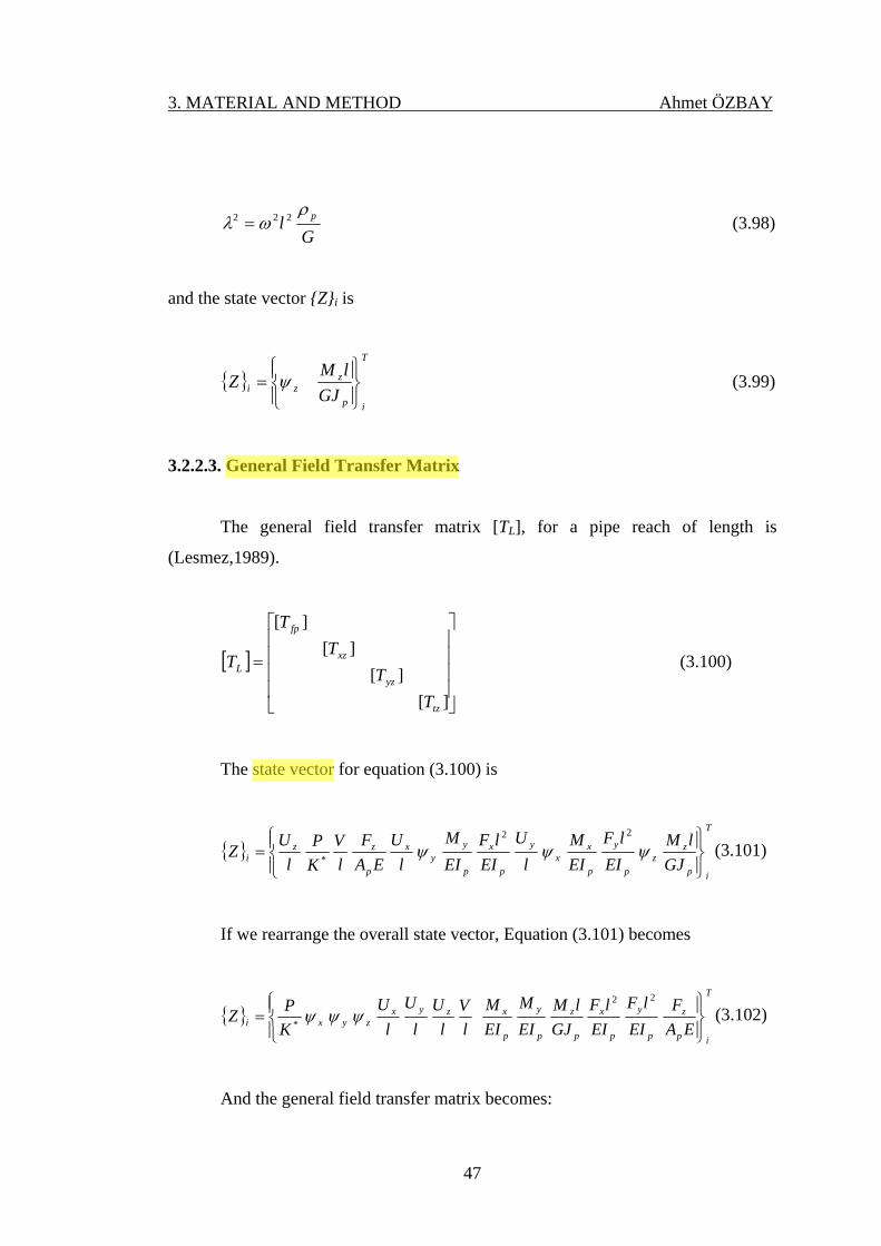
3. MATERIAL AND METHOD Ahmet ÖZBAY
47
Gl pρωλ 222 = (3.98)
and the state vector Zi is
T
ip
zzi GJ
lMZ⎪⎭
⎪⎬⎫
⎪⎩
⎪⎨⎧
= ψ (3.99)
3.2.2.3. General Field Transfer Matrix
The general field transfer matrix [TL], for a pipe reach of length is
(Lesmez,1989).
[ ]⎥⎥⎥⎥
⎦
⎤
⎢⎢⎢⎢
⎣
⎡
=
][][
][][
tz
yz
xz
fp
L
TT
TT
T (3.100)
The state vector for equation (3.100) is
T
ip
zz
p
y
p
xx
y
p
x
p
yy
x
p
zzi GJ
lMEI
lFEIM
lU
EIlF
EIM
lU
EAF
lV
KP
lU
Z⎪⎭
⎪⎬⎫
⎪⎩
⎪⎨⎧
= ψψψ22
*(3.101)
If we rearrange the overall state vector, Equation (3.101) becomes
T
ip
z
p
y
p
x
p
z
p
y
p
xzyxzyxi EA
FEI
lFEI
lFGJ
lMEIM
EIM
lV
lU
lU
lU
KPZ
⎪⎭
⎪⎬⎫
⎪⎩
⎪⎨⎧
=22
* ψψψ (3.102)
And the general field transfer matrix becomes:
ITD
Highlight
ITD
Highlight
ITD
Text Box
l
ITD
Text Box
l
ITD
Text Box
14 13 12 11 10 9 8 7 6 5 4 3 2 1
ITD
Text Box
4 12 8 14 7 11 3 1 9 5 13 6 10 2
ITD
Text Box
14 13 12 11 10 9 8 7 6 5 4 3 2 1

3. MATERIAL AND METHOD Ahmet ÖZBAY
48
[ ] 1−= iLi ZTZ (3.103)
or
[ ] [ ] [ ] [ ][ ] [ ] [ ] [ ]
[ ] [ ] [ ] [ ][ ] [ ]
[ ] [ ] [ ] [ ][ ] [ ] [ ] [ ]
[ ] [ ] [ ] [ ][ ] [ ] [ ] [ ]
[ ] [ ] [ ] [ ][ ] [ ] [ ] [ ]
[ ] [ ][ ] [ ] [ ] [ ]
[ ] [ ] [ ] [ ][ ] [ ] [ ] [ ]
1
2
2
*
44434142
44434142
44434142
2221
34333132
34333132
34333132
14131112
14131112
14131112
1211
24232122
24232122
24232122
2
2
*
00000000000000000000000000000000000000000000000000000000000000
00000000000000000000
0000000000000000000000000000000000000000000000000000
0000000000
−⎪⎪⎪⎪⎪⎪⎪⎪⎪⎪⎪⎪⎪⎪⎪⎪
⎭
⎪⎪⎪⎪⎪⎪⎪⎪⎪⎪⎪⎪⎪⎪⎪⎪
⎬
⎫
⎪⎪⎪⎪⎪⎪⎪⎪⎪⎪⎪⎪⎪⎪⎪⎪
⎩
⎪⎪⎪⎪⎪⎪⎪⎪⎪⎪⎪⎪⎪⎪⎪⎪
⎨
⎧
⎥⎥⎥⎥⎥⎥⎥⎥⎥⎥⎥⎥⎥⎥⎥⎥⎥⎥⎥⎥
⎦
⎤
⎢⎢⎢⎢⎢⎢⎢⎢⎢⎢⎢⎢⎢⎢⎢⎢⎢⎢⎢⎢
⎣
⎡
=
⎪⎪⎪⎪⎪⎪⎪⎪⎪⎪⎪⎪⎪⎪⎪⎪
⎭
⎪⎪⎪⎪⎪⎪⎪⎪⎪⎪⎪⎪⎪⎪⎪⎪
⎬
⎫
⎪⎪⎪⎪⎪⎪⎪⎪⎪⎪⎪⎪⎪⎪⎪⎪
⎩
⎪⎪⎪⎪⎪⎪⎪⎪⎪⎪⎪⎪⎪⎪⎪⎪
⎨
⎧
ip
z
p
y
p
x
p
z
p
y
p
x
z
y
x
z
y
x
fpfpfpfp
yzyzyzyz
xzxzxzxz
tztz
xzxzxzxz
yzyzyzyz
fpfpfpfp
fpfpfpfp
yzyzyzyz
xzxzxzxz
tztz
xzxzxzxz
yxyzyzyz
fpfpfpfp
ip
z
p
y
p
x
p
z
p
y
p
x
z
y
x
z
y
x
EAF
EIlF
EIlF
GJlM
EIMEIMlVl
Ul
Ul
U
KP
TTTTTTTT
TTTTTT
TTTTTTTT
TTTTTTTT
TTTTTTTT
TTTTTT
TTTTTTTT
EAF
EIlF
EIlF
GJlM
EIMEIMlVl
Ul
Ul
U
KP
ψψψ
ψψψ
(3.104)
3.2.2.4. Point Matrices
Field transfer matrices for each pipe section are connected by three types of
point transfer matrices which are bend, spring and mass point matrices. Valves,
accumulators and control instrumentation can be modeled as concentrated or point
masses. In this section bend and spring point matrices will be outlined.
ITD
Rectangle
ITD
Highlight
ITD
Highlight
ITD
Highlight
ITD
Highlight
ITD
Highlight
ITD
Highlight
ITD
Highlight
ITD
Highlight
ITD
Highlight
ITD
Highlight
ITD
Highlight
ITD
Text Box
14 13 12 11 10 9 8 7 6 5 4 3 2 1
ITD
Note
Tyz
ITD
Rectangle
ITD
Rectangle
ITD
Line
ITD
Line

3. MATERIAL AND METHOD Ahmet ÖZBAY
49
3.2.2.4.(1). Bend Point Matrix
A piping system in two or three dimensional space can be treated as a
collection of straight pipe reaches, differing in orientation and joined end-to-end. The
difference in orientation generates junction coupling of the fluid pressure and of the
pipe wail moments and forces between the reaches. The junction itself is treated as a
discontinuity with negligible mass and length. Equilibrium and continuity
relationships constitute the basis for point matrices at bends (Lesmez,1989).
Pipe bends or elbows can be considered as a velocity discontinuity where the
direction of fluid flow changes and pressure inside the piping exerts a force on the
pipe wall.
Figure 3.17. Sign convention for a bend.
The sate vectors to the right and left of point i, ZiR and Zi
L can be related by a
bend point matrix.
[ ] Lii
BL
Ri ZPZ = (3.105)
Bend point matrix [ ]iBLP may be derived for rotation about z- axis
L
i-1 i
R
α
i+1
ITD
Highlight
ITD
Highlight
ITD
Highlight
ITD
Highlight
ITD
Highlight
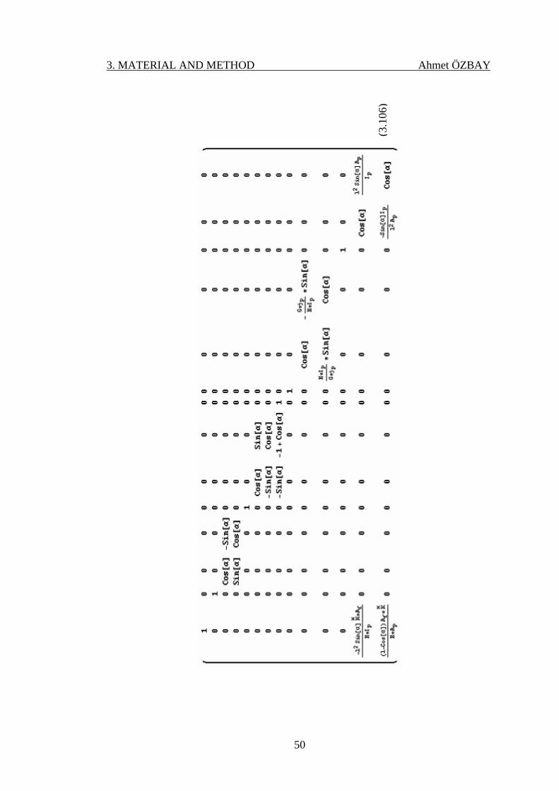
3. MATERIAL AND METHOD Ahmet ÖZBAY
50
(3.1
06)
ITD
Oval

3. MATERIAL AND METHOD Ahmet ÖZBAY
51
for rotation about y- axis
(3.1
07)
ITD
Highlight
ITD
Oval
ITD
Text Box
negative rotation about x

3. MATERIAL AND METHOD Ahmet ÖZBAY
52
for rotation about x- axis
(3.1
08)
ITD
Highlight
ITD
Oval
ITD
Text Box
negative rotation about y

3. MATERIAL AND METHOD Ahmet ÖZBAY
53
3.2.2.4.(2). Spring Point Matrix
Piping systems generally are supported at several locations, restricting motion
partially or totally, or they may be placed on an elastic foundation. The elastic
foundation can be represented by springs. Each spring can be modeled as a point
matrix (Lesmez, 1989).
Figure 3.18. shows the pipe reach has a spring support and is vibrating in the
y-z plane. The state vectors to the right and left of point i, RiZ and L
iZ can again
be related by a point matrix. Where ki is the stiffness of the spring.
Figure 3.18. Forces at spring
[ ] Lii
SL
Ri ZPZ = (3.109)
Spring point matrix is given as
x y
z
i-1 i
ki
RiZ
LiZ
RiFy
RiMx
RiFy
LiFy
LiMx
LiFy
i+1
kiUyi=Spring force
ITD
Highlight
ITD
Highlight
ITD
Highlight
ITD
Highlight

3. MATERIAL AND METHOD Ahmet ÖZBAY
54
(3.1
10)

3. MATERIAL AND METHOD Ahmet ÖZBAY
55
3.2.2.5. Boundary Conditions
Fixed-Fixed and Fixed-Free boundary conditions for structural, open-closed
and closed-open boundary conditions for liquid are examined in this part. The state
vector becomes for fixed-open end
ip
z
p
y
p
x
p
z
p
y
p
x
ip
z
p
y
p
x
p
z
p
y
p
x
z
y
x
z
y
x
EAF
EIlF
EIlF
GJlM
EIMEIMlV
EAF
EIlF
EIlF
GJlM
EIMEIMlVl
Ul
Ul
U
KP
⎪⎪⎪⎪⎪⎪⎪⎪⎪⎪⎪⎪⎪⎪⎪⎪
⎭
⎪⎪⎪⎪⎪⎪⎪⎪⎪⎪⎪⎪⎪⎪⎪⎪
⎬
⎫
⎪⎪⎪⎪⎪⎪⎪⎪⎪⎪⎪⎪⎪⎪⎪⎪
⎩
⎪⎪⎪⎪⎪⎪⎪⎪⎪⎪⎪⎪⎪⎪⎪⎪
⎨
⎧
=
⎪⎪⎪⎪⎪⎪⎪⎪⎪⎪⎪⎪⎪⎪⎪⎪
⎭
⎪⎪⎪⎪⎪⎪⎪⎪⎪⎪⎪⎪⎪⎪⎪⎪
⎬
⎫
⎪⎪⎪⎪⎪⎪⎪⎪⎪⎪⎪⎪⎪⎪⎪⎪
⎩
⎪⎪⎪⎪⎪⎪⎪⎪⎪⎪⎪⎪⎪⎪⎪⎪
⎨
⎧
2
2
2
2
*
0
0
0
0000
ψψψ
(3.111)
ITD
Highlight
ITD
Highlight
ITD
Highlight
ITD
Highlight
ITD
Highlight
ITD
Highlight
ITD
Highlight
ITD
Highlight
ITD
Highlight
ITD
Highlight

3. MATERIAL AND METHOD Ahmet ÖZBAY
56
for fixed-closed end
ip
z
p
y
p
x
p
z
p
y
p
x
ip
z
p
y
p
x
p
z
p
y
p
x
z
y
x
z
y
x
EAF
EIlF
EIlF
GJlM
EIMEIM
KP
EAF
EIlF
EIlF
GJlM
EIMEIMlVl
Ul
Ul
U
KP
⎪⎪⎪⎪⎪⎪⎪⎪⎪⎪⎪⎪⎪⎪⎪⎪
⎭
⎪⎪⎪⎪⎪⎪⎪⎪⎪⎪⎪⎪⎪⎪⎪⎪
⎬
⎫
⎪⎪⎪⎪⎪⎪⎪⎪⎪⎪⎪⎪⎪⎪⎪⎪
⎩
⎪⎪⎪⎪⎪⎪⎪⎪⎪⎪⎪⎪⎪⎪⎪⎪
⎨
⎧
=
⎪⎪⎪⎪⎪⎪⎪⎪⎪⎪⎪⎪⎪⎪⎪⎪
⎭
⎪⎪⎪⎪⎪⎪⎪⎪⎪⎪⎪⎪⎪⎪⎪⎪
⎬
⎫
⎪⎪⎪⎪⎪⎪⎪⎪⎪⎪⎪⎪⎪⎪⎪⎪
⎩
⎪⎪⎪⎪⎪⎪⎪⎪⎪⎪⎪⎪⎪⎪⎪⎪
⎨
⎧
2
2
*
2
2
*
0
0
0
0
000
ψψψ
(3.112)
for free-closed end
i
z
y
x
z
y
x
ip
z
p
y
p
x
p
z
p
y
p
x
z
y
x
z
y
x
lUl
Ul
U
KP
EAF
EIlF
EIlF
GJlM
EIMEIMlVl
Ul
Ul
U
KP
⎪⎪⎪⎪⎪⎪⎪⎪⎪⎪⎪⎪⎪⎪⎪⎪
⎭
⎪⎪⎪⎪⎪⎪⎪⎪⎪⎪⎪⎪⎪⎪⎪⎪
⎬
⎫
⎪⎪⎪⎪⎪⎪⎪⎪⎪⎪⎪⎪⎪⎪⎪⎪
⎩
⎪⎪⎪⎪⎪⎪⎪⎪⎪⎪⎪⎪⎪⎪⎪⎪
⎨
⎧
=
⎪⎪⎪⎪⎪⎪⎪⎪⎪⎪⎪⎪⎪⎪⎪⎪
⎭
⎪⎪⎪⎪⎪⎪⎪⎪⎪⎪⎪⎪⎪⎪⎪⎪
⎬
⎫
⎪⎪⎪⎪⎪⎪⎪⎪⎪⎪⎪⎪⎪⎪⎪⎪
⎩
⎪⎪⎪⎪⎪⎪⎪⎪⎪⎪⎪⎪⎪⎪⎪⎪
⎨
⎧
0
0
0
0
0
0
0
*
2
2
*
ψψψ
ψψψ
(3.113)
ITD
Highlight
ITD
Highlight
ITD
Highlight
ITD
Highlight
ITD
Highlight
ITD
Highlight
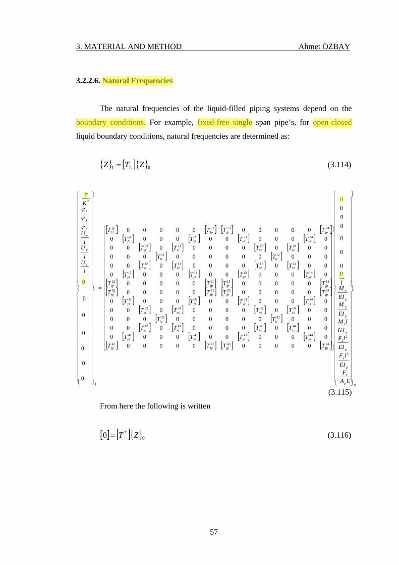
3. MATERIAL AND METHOD Ahmet ÖZBAY
57
3.2.2.6. Natural Frequencies
The natural frequencies of the liquid-filled piping systems depend on the
boundary conditions. For example, fixed-free single span pipe’s, for open-closed
liquid boundary conditions, natural frequencies are determined as:
[ ] 01 ZTZ L= (3.114)
[ ] [ ] [ ] [ ][ ] [ ] [ ] [ ]
[ ] [ ] [ ] [ ][ ] [ ]
[ ] [ ] [ ] [ ][ ] [ ] [ ] [ ]
[ ] [ ] [ ] [ ][ ] [ ] [ ] [ ]
[ ] [ ] [ ] [ ][ ] [ ] [ ] [ ]
[ ] [ ][ ] [ ] [ ] [ ]
[ ] [ ] [ ] [ ][ ] [ ] [ ] [ ]
0
2
2
44434142
44434142
44434142
2221
34333132
34333132
34333132
14131112
14131112
14131112
1211
24232122
24232122
24232122
1
*
0
0
0
0000
00000000000000000000000000000000000000000000000000000000000000
00000000000000000000
0000000000000000000000000000000000000000000000000000
0000000000
0
0
0
0
0
0
0
⎪⎪⎪⎪⎪⎪⎪⎪⎪⎪⎪⎪⎪⎪⎪⎪
⎭
⎪⎪⎪⎪⎪⎪⎪⎪⎪⎪⎪⎪⎪⎪⎪⎪
⎬
⎫
⎪⎪⎪⎪⎪⎪⎪⎪⎪⎪⎪⎪⎪⎪⎪⎪
⎩
⎪⎪⎪⎪⎪⎪⎪⎪⎪⎪⎪⎪⎪⎪⎪⎪
⎨
⎧
⎥⎥⎥⎥⎥⎥⎥⎥⎥⎥⎥⎥⎥⎥⎥⎥⎥⎥⎥⎥
⎦
⎤
⎢⎢⎢⎢⎢⎢⎢⎢⎢⎢⎢⎢⎢⎢⎢⎢⎢⎢⎢⎢
⎣
⎡
=
⎪⎪⎪⎪⎪⎪⎪⎪⎪⎪⎪⎪⎪⎪⎪⎪
⎭
⎪⎪⎪⎪⎪⎪⎪⎪⎪⎪⎪⎪⎪⎪⎪⎪
⎬
⎫
⎪⎪⎪⎪⎪⎪⎪⎪⎪⎪⎪⎪⎪⎪⎪⎪
⎩
⎪⎪⎪⎪⎪⎪⎪⎪⎪⎪⎪⎪⎪⎪⎪⎪
⎨
⎧
EAF
EIlF
EIlF
GJlM
EIMEIMl
V
TTTTTTTT
TTTTTT
TTTTTTTT
TTTTTTTT
TTTTTTTT
TTTTTT
TTTTTTTT
lUl
Ul
U
KP
p
z
p
y
p
x
p
z
p
y
p
x
fpfpfpfp
yzyzyzyz
xzxzxzxz
tztz
xzxzxzxz
yzyzyzyz
fpfpfpfp
fpfpfpfp
yzyzyzyz
xzxzxzxz
tztz
xzxzxzxz
yxyzyzyz
fpfpfpfp
z
y
x
z
y
x
ψψψ
(3.115)
From here the following is written
[ ] [ ] 0*0 ZT= (3.116)
ITD
Highlight
ITD
Highlight
ITD
Highlight
ITD
Highlight
ITD
Highlight
ITD
Highlight
ITD
Text Box
Fixed open
ITD
Text Box
free closed
ITD
Highlight
ITD
Highlight
ITD
Line
ITD
Line
ITD
Line
ITD
Line
ITD
Line

3. MATERIAL AND METHOD Ahmet ÖZBAY
58
[ ] [ ][ ] [ ]
[ ] [ ][ ]
[ ] [ ][ ] [ ]
[ ] [ ]
⎪⎪⎪⎪⎪⎪⎪⎪⎪
⎭
⎪⎪⎪⎪⎪⎪⎪⎪⎪
⎬
⎫
⎪⎪⎪⎪⎪⎪⎪⎪⎪
⎩
⎪⎪⎪⎪⎪⎪⎪⎪⎪
⎨
⎧
⎥⎥⎥⎥⎥⎥⎥⎥⎥
⎦
⎤
⎢⎢⎢⎢⎢⎢⎢⎢⎢
⎣
⎡
=
⎪⎪⎪⎪
⎭
⎪⎪⎪⎪
⎬
⎫
⎪⎪⎪⎪
⎩
⎪⎪⎪⎪
⎨
⎧
EAF
EIlF
EIlF
GJlM
EIMEIMlV
TTTT
TTT
TTTT
TT
p
z
p
y
p
x
p
z
p
y
p
x
fpfp
yzyz
xzxz
tz
xzxz
yzyz
fpfp
2
2
4443
4443
4443
22
3433
3433
3433
1 0000000000000000000000000000000
00000
0000000
(3.117)
[ ]*T is called eigen matrix and the frequencies satisfying the above condition
by making the determinant of the eigen matrix zero correspond to the natural
frequencies.
3.2.2.7. Vibration of a Pipe on Elastic Foundation
The field transfer matrices for pipe on elastic foundation are same with the
single straight pipe. Also the general field transfer matrix was composed of same
four sub matrices: longitudinal vibration of the liquid and pipe wall, transverse
vibration in the x-z as well as in the y-z planes and torsional vibration about the z-
axis. The general field transfer matrix expression is given in Equation (3.104).
Only the parameters σ, τ and γ are different in transverse vibration in the x-z and in
the y-z planes.
ITD
Highlight
ITD
Highlight
ITD
Highlight
ITD
Highlight
ITD
Highlight
ITD
Highlight

3. MATERIAL AND METHOD Ahmet ÖZBAY
59
22)(
lGA
AA
sp
ffpp
κωρρ
σΓ−+
= (3.118)
2*2)(
lEI
II
p
ffpp Γ−+=
ωρρτ (3.119)
42)(
lEI
AA
p
ffpp Γ−+=
ωρργ (3.120)
Where Γ is distributed foundation stiffness.
ITD
Highlight
ITD
Highlight

4. RESULTS AND DISCUSSION Ahmet ÖZBAY
60
4. RESULTS AND DISCUSSION
The objective of this chapter is to present both the theoretical based on the
transfer matrix method (TMM) and experimental results of this study. The results
obtained in this work are verified by both finite element solution using ANSYS and
some results available in the literature. It may be noted that since ANSYS neglects
the effect of bulk modulus of the fluid, natural frequencies evaluated by the ANSYS
in just the structural modes are used for comparisons.
The fundamental frequency of the system in liquid mode at Open-Closed
boundary conditions is given by
l
cf f
f 4= (3.1)
where ff is the fundamental frequency of the liquid, cf is the coupled wave speed and l
is the length of the pipe. By using both Equations (3.1.) and (3.22.) coupled wave
speed cf may be calculated as 1405 m/s for steel pipe and as 1279 m/s for copper
pipe.
Akdoğan (1992) also studied a single-spanned pipe filled a light fluid at
various end conditions with the help of the transfer matrix method offered in this
study. Comparison of the present results with Akdoğan’s (1992) results is given in
Tables 4.1. and 4.2. From those tables an excellent agreement is observed between
the fundamental frequencies in both structural and fluid modes.
ITD
Highlight
ITD
Highlight
ITD
Highlight
ITD
Highlight
ITD
Highlight
ITD
Highlight
ITD
Highlight
ITD
Highlight
ITD
Highlight
ITD
Highlight
ITD
Highlight
ITD
Highlight
ITD
Rectangle

4. RESULTS AND DISCUSSION Ahmet ÖZBAY
61
Table 4.1. Comparison of the present theoretical natural frequencies (rad/s) of 5m-length copper pipe filled by the air with the literature(Fixed-Fixed and Open-Closed)
(E=117 GPa, ρp=8940 kg/m3, K=0.14 GPa, ρf:=1.2 kg/m3)
Modes Present Study
(TMM)
Akdoğan
(1992)
Equation
(3.1)
Structural 31.1377 31.138 -
Structural 85.7764 85.7764 -
Fluid 107.0931 106.86 106.869
Structural 168.01 168.01 -
Structural 277.425 277.43 -
Fluid 320.68 320.58 320.606
Structural 413.876 413.88 -
Fluid 534.378 534.52 534.343
Structural 577.163 577.16 -
Fluid 748.102 751.13 748.08
Table 4.2. Comparison of the present theoretical natural frequencies (rad/s) of 5m-length copper pipe filled by the air with the literature (Fixed-Fixed and Open-Closed)
(E=117 GPa, ρp=8940 kg/m3, K=0.14 GPa, ρf:=1.2 kg/m3)
Modes Present Study
(TMM)
Akdoğan
(1992) Equation (3.1)
Structural 4.89561 4.896 -
Structural 30.6702 30.670 -
Structural 85.8322 85.832 -
Fluid 106.865 106.86 106.869
Structural 168.068 168.07 -
Structural 277.551 277.55 -
Fluid 320.609 320.59 320.606
Structural 414.105 414.10 -
Fluid 534.34 534.52 534.343
Structural 577.539 577.54 -
ITD
Highlight
ITD
Highlight
ITD
Highlight
ITD
Highlight

4. RESULTS AND DISCUSSION Ahmet ÖZBAY
62
Earlier than the case studies considered in this work, the soundness of the
present experiments is confirmed by a few tests at just structural fixed-fixed ends.
As mentioned in the previous chapter, impact hammer test is used together
with FFT analyzer to determine the natural frequencies of the system in the structural
mode. The measurements are taken in different directions and locations. The liquid
natural frequencies are measured by using both the pressure transmitter and the
external shaker. The liquid inside the pipe is excited at the natural frequency in the
liquid mode by the external shaker. The pressure was fluctuated with large amplitude
when the shaker excited at liquid natural frequency. Comparison of the experimental
frequency measured in liquid mode is made with Equation (3.1.)
To explain the experimental procedure let’s consider 25m-length steel pipe.
The fundamental frequency of the liquid may be calculated in an analytical manner
as ff =5.936Hz by using Equation (3.1.) At normal conditions (without any external
disturbance) the pressure inside the pipe is about 2bar. When the pipe is excited by
an external harmonic force, then the amplitude of the inside pressure gets start to
fluctuate about the pressure of 2bar. As the amplitude of the harmonic force
increases, the amplitude of the inside pressure increases. When the external disturbed
frequency near the natural frequency of the liquid inside the pipe, due to the
resonance phenomena amplitudes become very large. This is clearly shown in Figure
4.1 and 4.2. shows the pressure values for definite time period while the excitation
frequency is near 6.0375 Hz.
ITD
Highlight
ITD
Highlight
ITD
Highlight
ITD
Highlight
ITD
Highlight
ITD
Highlight
ITD
Highlight
ITD
Highlight
ITD
Highlight
ITD
Highlight

4. RESULTS AND DISCUSSION Ahmet ÖZBAY
63
-6
-4
-2
0
2
4
6
8
10
1 125 249 373 497 621 745 869 993 1117 1241 1365 1489 1613
Time (s)
Pressure (1/10 Bar)
Figure 4.1. Experimental pressure-time history of 25m-length steel pipe with fixed-
fixed ends at different external excitation frequencies.
-6
-4
-2
0
2
4
6
8
10
580
595
610
625
640
655
670
685
700
715
730
745
760
775
790
805
Time (s)
Pressure (1/10 Bar)
Figure 4.2. Experimental pressure-time history when external excitation frequency
is equal to the liquid frequency (6.0375 Hz).

4. RESULTS AND DISCUSSION Ahmet ÖZBAY
64
After verifying the present theoretical and experimental results a few case studies
are considered in this section. In the case studies considered five different
configurations of piping systems made of either one inch-nominal diameter copper or
two inch-nominal diameter steel such as
• Single-spanned
• L-Bended
• Z-Bended
• U-Bended
• 3-D Bended
are studied with two structural boundary conditions namely fixed-fixed and fixed-
free. Fluid boundary conditions are assumed to be closed at both ends. As a light
fluid both the air and the water are considered. Material and geometrical properties
of the pipes are presented in Tables 3.1 and 3.2. The physical properties of the water
considered in this study are given by Table 3.3.
4.1. Single-Spanned Pipe with Various End Conditions
Fixed-fixed, fixed-free, and intermediate rigid support applications are
examined for a single-spanned pipe.
Figure 4.3. Single-spanned pipe supported at two ends
L
ITD
Highlight
ITD
Highlight
ITD
Highlight
ITD
Highlight
ITD
Highlight
ITD
Highlight
ITD
Highlight

4. RESULTS AND DISCUSSION Ahmet ÖZBAY
65
4.1.1. Fixed-Fixed Single-Spanned Pipe
In this section, the natural frequencies of 2m-length copper and 3.5m-length
steel pipes filled by both the air and the water are taken into consideration.
Table 4.3. Natural frequencies (Hz) of 2m-length copper pipe with the air (Fixed-Fixed and Open-Closed) Present Study
Modes TMM Experimental
ANSYS Equation
(3.1)
Structural 28.8841 27.06 29.004 -
Fluid 42.5994 - - 42.5217
Structural 79.3206 - 80.972 -
Fluid 127.591 - - 127.565
Structural 154.727 - 188.71 -
In ANSY solution of this problem the pipe is divided into ten elements which
are defined by element type Pipe 16. The source program and its numerical results
are presented in Appendix A.1.
Figure 4.4. PIPE16 - Elastic straight pipe
ITD
Highlight
ITD
Highlight
ITD
Highlight
ITD
Highlight
ITD
Highlight
ITD
Highlight
ITD
Highlight
ITD
Highlight
ITD
Highlight
ITD
Highlight
ITD
Highlight

4. RESULTS AND DISCUSSION Ahmet ÖZBAY
66
Figures 4.5, 4.6, and 4.7 shows the FFT spectrum of fixed-fixed single-
spanned 2m-length copper pipe with the air in tangential, radial and axial directions,
respectively. The results taken from different directions are quite close to each other
and the distinct peak near 27 Hz verifies the tabulated TMM and ANSYS results.
Figure 4.5. FFT Spectrum in tangential direction of fixed-fixed single -spanned 2m-
length copper pipe with the air
ITD
Highlight
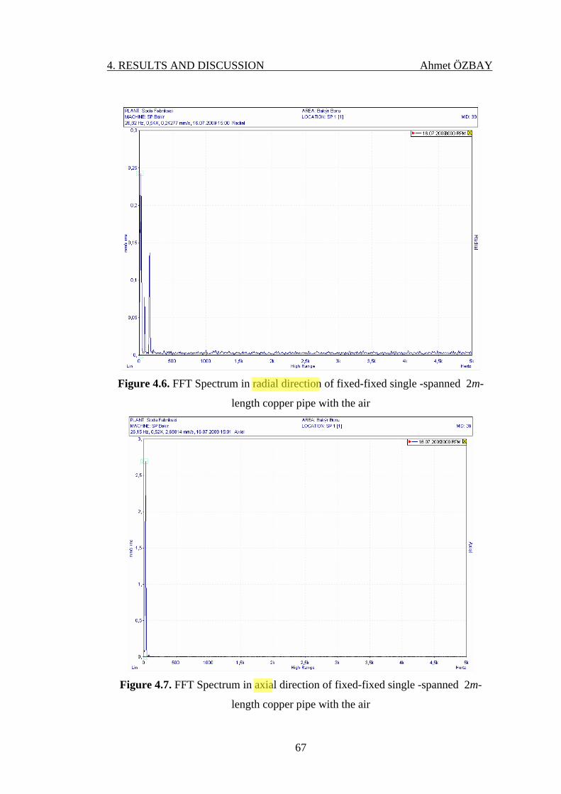
4. RESULTS AND DISCUSSION Ahmet ÖZBAY
67
Figure 4.6. FFT Spectrum in radial direction of fixed-fixed single -spanned 2m-
length copper pipe with the air
Figure 4.7. FFT Spectrum in axial direction of fixed-fixed single -spanned 2m-
length copper pipe with the air
ITD
Highlight
ITD
Highlight

4. RESULTS AND DISCUSSION Ahmet ÖZBAY
68
The natural frequencies of 2m-length copper pipe with the water for Fixed-
Fixed/Open-Closed conditions are listed in Table 4.4. The FFT spectrums of this
example in axial and tangential directions are presented by Figures 4.8 and 4.9,
respectively.
Table 4.4. Natural frequencies (Hz) of 2m-length copper pipe with the water (Fixed-Fixed and Open-Closed)
Present Study Modes
TMM ExperimentalANSYS
Equation
(3.1)
Structural 21.8473 21.95 21.973 -
Structural 60.0014 - 61.243 -
Structural 157,057 - 142.73 -
Fluid 164 - - 160
ITD
Highlight
ITD
Highlight
ITD
Highlight
ITD
Highlight
ITD
Highlight
ITD
Highlight

4. RESULTS AND DISCUSSION Ahmet ÖZBAY
69
Figure 4.8. FFT spectrum in axial directions at two locations of fixed-fixed single -
spanned 2m-length copper pipe with the water
Figure 4.9. FFT Spectrum in tangential direction of fixed-fixed single -spanned 2m-
length copper pipe with the water

4. RESULTS AND DISCUSSION Ahmet ÖZBAY
70
Tables 4.5 and 4.6 presents the natural frequencies of 3.5m-length steel pipe
with both the air and the water, respectively. The boundary conditions are assumed to
be fixed-fixed for the pipe and Open-Closed for the liquid.
Table 4.5. Natural frequencies (Hz) of 3.5m-length steel pipe with the air (Fixed-Fixed and Open-Closed)
Modes Present Study
(TMM) ANSYS Equation (3.1)
Structural 21.9154 22.007 -
Structural 60.102 61.369 -
Fluid 101.089 - 100.416
Table 4.6. Natural frequencies (Hz) of 3.5m-length steel pipe with the water (Fixed-Fixed and Open-Closed)
Modes Present Study
(TMM) ANSYS Equation (3.1)
Fluid 24.3082 - 24.2981
Structural 26.4215 26.532 -
Fluid 72.4528 - 72.8944
Structural 72.8978 73.990 -
Fluid 121.492 - 121.491
4.1.2. Fixed-Free Single -Spanned Pipe
Here 3m-length copper and steel pipes filled by both the air and the water are
studied theoretically. Results are given by Tables 4.7-4.10. Present results show a
good harmony with the ANSYS’s results.
ITD
Highlight

4. RESULTS AND DISCUSSION Ahmet ÖZBAY
71
Table 4.7. Natural frequencies (Hz) of 3m-length copper pipe with the air (Fixed-Free and Open-Closed)
Modes Present Study
(TMM) ANSYS Equation (3.1)
Structural 2.02316 2.0234 -
Structural 12.6681 12.710 -
Fluid 28.347 - 28.348
Structural 35.4226 35.874 -
Fluid 85.0441 - 85.0433
Fluid 141.738 - 141.739
Table 4.8. Natural frequencies (Hz) of 3m-length copper pipe with the water (Fixed-Free and Open-Closed)
Modes Present Study
(TMM) ANSYS Equation (3.1)
Structural 1.53023 1.5304 -
Structural 9.58195 9.6134 -
Structural 26.7944 27.134 -
Fluid 106.665 - 106.665
Table 4.9. Natural frequencies (Hz) of 3m-length steel pipe with the air (Fixed-Free and Open-Closed)
Modes Present Study
(TMM) ANSYS Equation (3.1)
Structural 40.918 40.921 -
Fluid 178.114 - 178.057
Structural 255.504 256.39 -
Fluid 534.344 - 534.171
Structural 711.298 721.12 -
Fluid 890.571 - 890.285
ITD
Highlight
ITD
Highlight
ITD
Highlight
ITD
Highlight
ITD
Highlight
ITD
Highlight
ITD
Highlight
ITD
Highlight
ITD
Highlight
ITD
Highlight
ITD
Highlight

4. RESULTS AND DISCUSSION Ahmet ÖZBAY
72
Table 4.10. Natural frequencies (Hz) of 3m-length steel pipe with the water (Fixed-Free and Open-Closed)
Modes Present Study
(TMM) ANSYS Equation (3.1)
Structural 33.939 33.941 -
Structural 211.948 212.66 -
Structural 590.144 598.09 -
Fluid 745.591 - 745.405
4.1.3. Single -Spanned Pipe with Intermediate Rigid Support
Both copper and steel pipes with the air or the water are again examined for
fixed-fixed and Open-Closed boundary conditions. The total length of the pipe is 7m
for the copper pipe and 6m for the steel pipe. The pipe wall displacement at the
middle of the pipe is restricted in x and y directions.
Figure 4.10. Single -spanned pipe with rigid support
L/2
L/2
ITD
Highlight
ITD
Highlight
ITD
Highlight
ITD
Highlight
ITD
Highlight
ITD
Highlight
ITD
Highlight
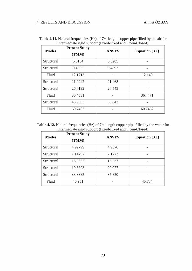
4. RESULTS AND DISCUSSION Ahmet ÖZBAY
73
Table 4.11. Natural frequencies (Hz) of 7m-length copper pipe filled by the air for intermediate rigid support (Fixed-Fixed and Open-Closed)
Modes Present Study
(TMM) ANSYS Equation (3.1)
Structural 6.5154 6.5285 -
Structural 9.4505 9.4893 -
Fluid 12.1713 - 12.149
Structural 21.0942 21.468 -
Structural 26.0192 26.545 -
Fluid 36.4531 - 36.4471
Structural 43.9503 50.043 -
Fluid 60.7483 - 60.7452
Table 4.12. Natural frequencies (Hz) of 7m-length copper pipe filled by the water for intermediate rigid support (Fixed-Fixed and Open-Closed)
Modes Present Study
(TMM) ANSYS Equation (3.1)
Structural 4.92799 4.9376 -
Structural 7.14797 7.1773 -
Structural 15.9552 16.237 -
Structural 19.6803 20.077 -
Structural 38.3385 37.850 -
Fluid 46.951 - 45.734

4. RESULTS AND DISCUSSION Ahmet ÖZBAY
74
Table 4.13. Natural frequencies (Hz) of 6m-length steel pipe filled by the air for intermediate rigid support (Fixed-Fixed and Open-Closed)
Modes Present Study
(TMM) ANSYS Equation (3.1)
Fluid 14.1784 - 14.1739
Structural 28.4835 28.541 -
Fluid 41.2327 - 42.5217
Structural 42.5231 41.408 -
Fluid 70.8704 - 70.8696
Structural 91.8079 93.547 -
Fluid 99.2181 - 99.2174
Table 4.14. Natural frequencies (Hz) of 6m-length steel pipe filled by the water for
intermediate rigid support (Fixed-Fixed and Open-Closed)
Modes Present Study
(TMM) ANSYS Equation (3.1)
Structural 23.626 23.673 -
Structural 34.2012 34.34 -
Fluid 59.6176 - 59.3174
Structural 76.1604 77.590 -
Fluid 177.994 - 177.952
4.2. Two Pipes with 90o-Bended (L-Bended Pipe)
Free vibration behavior of two pipes which are connected with 90-degrees
Bended Figure 4.11 is worked out both theoretically and experimentally for different
pipe materials, different fluids and different boundary conditions including the
intermediate rigid support.
ITD
Highlight
ITD
Highlight

4. RESULTS AND DISCUSSION Ahmet ÖZBAY
75
Figure 4.11. L-Bended pipe supported at two ends
In this case study, the steel and the cooper are chosen as the pipe materials,
and the air and the water are used as the fluids. Open-Closed ends are used as fluid
boundary conditions.
4.2.1. L-Bended Pipe with Fixed-Free Ends
In these examples L1 = L2 =2.5m for the steel pipe and L1 = L2 =1m for the
copper pipe.
Natural frequencies of L-Bended fixed-free pipe made of steel are presented
in Table 4.15 for the air and Table 4.16 for the water, respectively.
L1 L2
ITD
Highlight
ITD
Highlight
ITD
Highlight

4. RESULTS AND DISCUSSION Ahmet ÖZBAY
76
Table 4.15. Natural frequencies (Hz) of L-Bended steel pipe with the air (Fixed-Closed / Free-Closed)
Modes Present Study
(TMM) ANSYS Equation (3.1)
Structural 2.45193 2.5768 -
Structural 2.5768 2.7227 -
Structural 6.84158 7.1050 -
Structural 7.10453 7.4044 -
Fluid 19.5947 - 17.0087
Structural 36.2799 36.354 -
Structural 36.44 36.531 -
Fluid 51.1022 - 51.0261
Structural 52.8358 53.022 -
Structural 54.1443 53.411 -
Fluid 85.5964 - 85.0435
Table 4.16. Natural frequencies (Hz) of L-Bended steel pipe with the water (Fixed-Closed / Free-Closed)
Modes Present Study
(TMM) ANSYS Equation (3.1)
Structural 2.13731 2.1373 -
Structural 2.25819 2.2583 -
Structural 5.89353 5.8931 -
Structural 6.13976 6.1414 -
Structural 30.1096 30.153 -
Structural 30.2118 30.300 -
Structural 43.8803 43.978 -
Structural 43.9479 44.301 -
Fluid 79.2599 - 70.2914
ITD
Highlight
ITD
Highlight
ITD
Highlight
ITD
Highlight
ITD
Highlight
ITD
Highlight

4. RESULTS AND DISCUSSION Ahmet ÖZBAY
77
Natural frequencies of L-Bended fixed-free pipe made of copper are
presented in Table 4.17 for the air and Table 4.18 for the water, respectively.
Table 4.17. Natural Frequencies (Hz) of L-Bended copper pipe with the air (Fixed-Closed / Free-Closed)
Modes Present Study
(TMM) ANSYS Equation (3.1)
Structural 5.15935 5.6669 -
Structural 5.66703 6.0667 -
Structural 14.8292 15.692 -
Structural 15.6908 16.487 -
Fluid 51.8677 - 42.5217
Structural 80.5901 80.754 -
Structural 81.1612 81.254 -
Table 4.18. Natural Frequencies (Hz) of L-Bended copper pipe with the water (Fixed-Closed / Free-Closed)
Modes Present Study
(TMM) ANSYS Equation (3.1)
Structural 4.2864 4.2862 -
Structural 4.58839 4.5886 -
Structural 11.8711 11.868 -
Structural 12.4678 12.470 -
Structural 61.0249 61.079 -
Structural 61.2718 61.457 -
Structural 88.8322 88.928 -
Structural 89.0154 89.668 -
Fluid 184.568 - 159.997
Structural 193.246 195.81 -
ITD
Highlight
ITD
Highlight
ITD
Highlight
ITD
Highlight
ITD
Highlight
ITD
Highlight
ITD
Highlight

4. RESULTS AND DISCUSSION Ahmet ÖZBAY
78
From Tables 4.17 and 4.18, for both the water and the air, a very good
harmony is observed between the present theoretical results and the finite element’s
solutions.
4.2.2. L-Bended Pipe with Fixed-Fixed Ends
A few of pipes with different lengths are studied in both theoretical and
experimental manner.
• L1 = L2 =2.4m for the steel pipe
• L1 = L2 =1m for the copper pipe.
• L1 = L2 =3.5m for the copper pipe.
The natural frequencies of L-Bended Steel Pipe (L1 = L2 = 2.4 m) with the
air (fixed-open / fixed-closed) are presented in Table 4.19. FFT spectrums in axial
directions at two locations are presented in Figure 4.12. Figure 4.13 shows the FFT
spectrum in radial direction of the same pipe.
Table 4.19. Natural frequencies (Hz) of L-Bended steel pipe with the air (Fixed-Open/ Fixed-Closed) (L1 = L2 = 2.4 m)
Present Study Modes
TMM ExperimentalANSYS
Equation
(3.1)
Structural 10.3506 10.00 10.352 -
Fluid 17.7185 - - 17.7174
Structural 38.6508 - 38.730 -
Structural 40.5088 - 40.600 -
Fluid 53.0942 - - 53.1522
Structural 55.7672 - 56.004 -
Structural 58.5156 - 58.757 -
Fluid 88.414 - - 88.587
ITD
Highlight
ITD
Highlight
ITD
Highlight
ITD
Highlight

4. RESULTS AND DISCUSSION Ahmet ÖZBAY
79
Figure 4.12. FFT Spectrum in axial direction at two locations of L-Bended steel
pipe with the air (Fixed-Open/ Fixed-Closed) (L1 = L2 = 2.4 m)

4. RESULTS AND DISCUSSION Ahmet ÖZBAY
80
Figure 4.13. FFT Spectrum in radial direction of L-Bended steel pipe with the air
(Fixed-Open/ Fixed-Closed) (L1 = L2 = 2.4 m)
The natural frequencies of L-Bended Steel Pipe (L1 = L2 = 2.4 m) with the
water (Fixed-Open/ Fixed-Closed) are presented in Table 4.20. In this example, two
fundamental frequencies in both structural and fluid modes are also determined
experimentally. For the fundamental frequency in structural mode, Figure 4.14 shows
the FFT spectrum in tangential direction of the same pipe. FFT spectrums in radial
direction at two locations are presented in Figure 4.15. For this problem, the source
program and its numerical results are presented in Appendix A.2.
ITD
Highlight
ITD
Highlight
ITD
Highlight

4. RESULTS AND DISCUSSION Ahmet ÖZBAY
81
Table 4.20. Natural frequencies (Hz) of L-Bended steel pipe with the water (Fixed-Open/ Fixed-Closed) (L1 = L2 = 2.4 m)
Present Study Modes
TMM ExperimentalANSYS
Equation
(3.1)
Structural 8.58553 9.16 8.5859 -
Structural 32.0602 - 32.124 -
Structural 33.608 - 33.675 -
Structural 46.257 - 46.451 -
Structural 48.5676 - 48.734 -
Fluid 73.3263 76.5333 - 73.2203
Structural 102.786 - 104.78 -
Figure 4.14. FFT Spectrum in tangential direction of L-Bended steel pipe with the
water (Fixed-Open/ Fixed-Closed) (L1 = L2 = 2.4 m)
ITD
Highlight
ITD
Highlight

4. RESULTS AND DISCUSSION Ahmet ÖZBAY
82
Figure 4.15. FFT Spectrums in radial direction at two locations of L-Bended steel
pipe with the water (Fixed-Open/ Fixed-Closed) (L1 = L2 = 2.4 m)
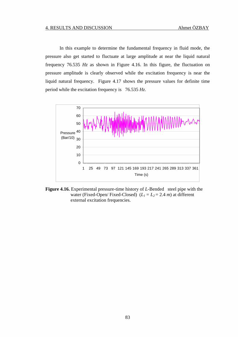
4. RESULTS AND DISCUSSION Ahmet ÖZBAY
83
In this example to determine the fundamental frequency in fluid mode, the
pressure also get started to fluctuate at large amplitude at near the liquid natural
frequency 76.535 Hz as shown in Figure 4.16. In this figure, the fluctuation on
pressure amplitude is clearly observed while the excitation frequency is near the
liquid natural frequency. Figure 4.17 shows the pressure values for definite time
period while the excitation frequency is 76.535 Hz.
0
10
20
30
40
50
60
70
1 25 49 73 97 121 145 169 193 217 241 265 289 313 337 361
Time (s)
Pressure (Bar/10)
Figure 4.16. Experimental pressure-time history of L-Bended steel pipe with the
water (Fixed-Open/ Fixed-Closed) (L1 = L2 = 2.4 m) at different external excitation frequencies.

4. RESULTS AND DISCUSSION Ahmet ÖZBAY
84
0
10
20
30
40
50
60
70
96 100 104 108 112 116 120 124 128 132 136 140 144
Time (s)
Pressure (Bar/10)
Figure 4.17. Experimental pressure-time history of L-Bended steel pipe with the
water (Fixed-Open/ Fixed-Closed) (L1 = L2 = 2.4 m) when external excitation frequency is equal to the liquid frequency (76.53 Hz).
As stated above, for fixed-fixed conditions, the L-Bended pipe made of the
copper is studied for two different lengths.
For L1 = L2 = 1 m and the air, both the theoretical and experimental results are
given in Table 4.21. The related FFT spectrums in both axial and tangential
directions are illustrated in Figure 4.18.
Table 4.21. Natural frequencies (Hz) of L-Bended copper pipe with the air (Fixed-Open/ Fixed-Closed) (L1 = L2 = 1 m)
Present Study Modes
TMM ExperimentalANSYS
Equation
(3.1)
Structural 21.1335 21.43 21.135 -
Fluid 42.5752 - - 42.5217
Structural 79.2158 - 79.376 -
Structural 82.8509 - 83.035 -
Structural 114.055 - 114.56 -
Structural 119.531 - 120.03 -
Fluid 127.231 - - 127.565
ITD
Highlight
ITD
Highlight

4. RESULTS AND DISCUSSION Ahmet ÖZBAY
85
Figure 4.18. FFT Spectrums in axial and tangential directions of L-Bended copper
pipe with the air (Fixed-Open/ Fixed-Closed) (L1 = L2 = 1 m)

4. RESULTS AND DISCUSSION Ahmet ÖZBAY
86
For L1 = L2 = 1m and the water, both the theoretical and experimental results
are given in Table 4.22. The related FFT spectrums in both axial and radial directions
are illustrated in Figure 4.19.
Table 4.22. Natural frequencies (Hz) of L-Bended copper pipe with the water (Fixed-Open/ Fixed-Closed) (L1 = L2 = 1 m)
Present Study Modes
TMM ExperimentalANSYS
Equation
(3.1)
Structural 15.986 15.75 15.986 -
Structural 59.9224 - 60.036 -
Structural 62.694 - 62.804 -
Structural 86.2861 - 86.645 -
Structural 90.5175 - 90.782 -
Fluid 163.045 - - 159.997
Structural 194.661 - 195.23 -
ITD
Highlight
ITD
Highlight

4. RESULTS AND DISCUSSION Ahmet ÖZBAY
87
Figure 4.19. FFT Spectrums in axial and radial directions of L-Bended copper
pipe with the water (Fixed-Open/ Fixed-Closed) (L1 = L2 = 1 m)
Natural frequencies of L-Bended copper pipe with the air (Fixed-Open/
Fixed-Closed) (L1 = L2 = 3.5 m) are studied by just theoretically and the results are
tabulated in Table 4.23.
Table 4.23. Natural frequencies (Hz) of L-Bended copper pipe with the air (Fixed-Open/ Fixed-Closed) (L1 = L2 = 3.5 m)
Modes Present Study
(TMM) ANSYS Equation (3.1)
Structural 1.72802 1.7283 -
Structural 6.51469 6.5275 -
Structural 6.81232 6.8270 -
Structural 9.44743 9.4862 -
Structural 9.85814 9.8955 -
Fluid 12.1644 - 12.149
Structural 21.086 21.460 -
Structural 21.3841 21.768 -

4. RESULTS AND DISCUSSION Ahmet ÖZBAY
88
Natural frequencies of L-Bended copper pipe with the water (Fixed-Open/
Fixed-Closed) (L1 = L2 = 3.5 m) are studied by both theoretically and experimentally.
In the experimental study, the fundamental frequency in fluid mode is measured.
Those frequencies are presented in Table 4.24. Figures 4.20 and 4.21 illustrate the
experimental pressure-time history of this pipe system at different external excitation
frequencies and when the external excitation frequency is equal to the fundamental
liquid frequency (44.55Hz).
Table 4.24. Natural frequencies (Hz) of L-Bended copper pipe with the water (Fixed-Open/ Fixed-Closed) (L1 = L2 = 3.5 m)
Present Study Modes
TMM Experimental ANSYS
Equation
(3.1)
Structural 1.30701 - 1.3072 -
Structural 4.92745 - 4.9371 -
Structural 5.15272 - 5.1636 -
Structural 7.14567 - 7.1749 -
Structural 7.45698 - 7.4845 -
Structural 15.9493 - 16.231 -
Structural 16.1761 - 16.464 -
Structural 19.6615 - 20.059 -
Structural 20.1198 - 20.374 -
Fluid 46.5979 44.55 - 45.7134
ITD
Highlight
ITD
Highlight
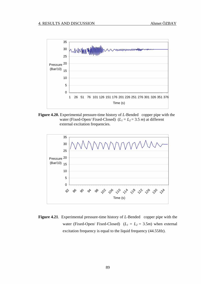
4. RESULTS AND DISCUSSION Ahmet ÖZBAY
89
0
5
10
15
20
25
30
35
1 26 51 76 101 126 151 176 201 226 251 276 301 326 351 376
Time (s)
Pressure (Bar/10)
Figure 4.20. Experimental pressure-time history of L-Bended copper pipe with the
water (Fixed-Open/ Fixed-Closed) (L1 = L2 = 3.5 m) at different external excitation frequencies.
0
5
10
15
20
25
30
35
82 86 90 94 98 102
106
110
114
118
122
126
130
134
Time (s)
Pressure (Bar/10)
Figure 4.21. Experimental pressure-time history of L-Bended copper pipe with the
water (Fixed-Open/ Fixed-Closed) (L1 = L2 = 3.5m) when external
excitation frequency is equal to the liquid frequency (44.55Hz).
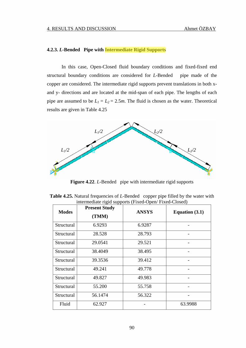
4. RESULTS AND DISCUSSION Ahmet ÖZBAY
90
4.2.3. L-Bended Pipe with Intermediate Rigid Supports
In this case, Open-Closed fluid boundary conditions and fixed-fixed end
structural boundary conditions are considered for L-Bended pipe made of the
copper are considered. The intermediate rigid supports prevent translations in both x-
and y- directions and are located at the mid-span of each pipe. The lengths of each
pipe are assumed to be L1 = L2 = 2.5m. The fluid is chosen as the water. Theoretical
results are given in Table 4.25
Figure 4.22. L-Bended pipe with intermediate rigid supports
Table 4.25. Natural frequencies of L-Bended copper pipe filled by the water with intermediate rigid supports (Fixed-Open/ Fixed-Closed)
Modes Present Study
(TMM) ANSYS Equation (3.1)
Structural 6.9293 6.9287 -
Structural 28.528 28.793 -
Structural 29.0541 29.521 -
Structural 38.4049 38.495 -
Structural 39.3536 39.412 -
Structural 49.241 49.778 -
Structural 49.827 49.983 -
Structural 55.200 55.758 -
Structural 56.1474 56.322 -
Fluid 62.927 - 63.9988
L1/2
L1/2 L2/2
L2/2
ITD
Highlight
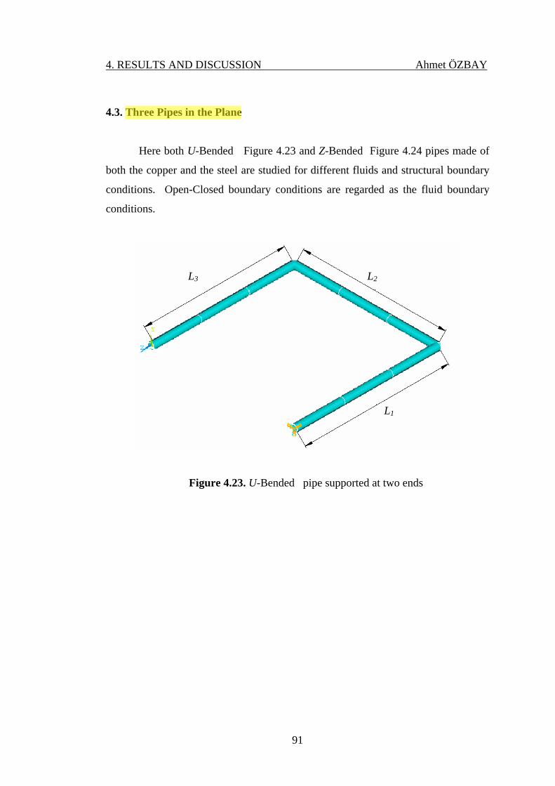
4. RESULTS AND DISCUSSION Ahmet ÖZBAY
91
4.3. Three Pipes in the Plane
Here both U-Bended Figure 4.23 and Z-Bended Figure 4.24 pipes made of
both the copper and the steel are studied for different fluids and structural boundary
conditions. Open-Closed boundary conditions are regarded as the fluid boundary
conditions.
Figure 4.23. U-Bended pipe supported at two ends
L3
L1
L2
ITD
Highlight

4. RESULTS AND DISCUSSION Ahmet ÖZBAY
92
Figure 4.24. Z-Bended Pipe supported at two ends
4.3.1. Z-Bended Pipe with Fixed-Free Ends
In this case study, the pipe material is determined as the steel. The length of
each pipe as assumed to be equal (L1 = L2 = L3=1.25m). Both the air and the water
are used as the fluids. Open-Closed fluid boundary conditions and fixed-free
structural end conditions are carried out. The theoretical results for the air are
presented in Table 4.26 and for the water are presented in Table 4.27.
L3
L2
L1
ITD
Highlight

4. RESULTS AND DISCUSSION Ahmet ÖZBAY
93
Table 4.26. Natural frequencies (Hz) of Z-Bended steel pipe with the air (Fixed-Closed / Free-Closed) (L1 = L2 = L3=1.25m)
Modes Present Study
(TMM) ANSYS Equation (3.1)
Structural 5.16198 5.4328 -
Structural 5.43299 5.7595 -
Fluid 17.8572 - 22.6783
Structural 22.1406 22.141 -
Structural 25.141 24.008 -
Structural 29.6929 30.807 -
Structural 30.8186 31.810 -
Fluid 73.5498 - 68.0348
Structural 143.529 143.83 -
Table 4.27. Natural frequencies (Hz) of Z-Bended steel pipe with the water (Fixed-Closed / Free-Closed) (L1 = L2 = L3=1.25m)
Modes Present Study
(TMM) ANSYS Equation (3.1)
Structural 4.50648 4.5061 -
Structural 4.77698 4.7770 -
Structural 18.3752 18.364 -
Structural 19.8433 19.913 -
Structural 26.3827 25.552 -
Fluid 102.021 - 94.9079
Structural 117.484 117.39 -
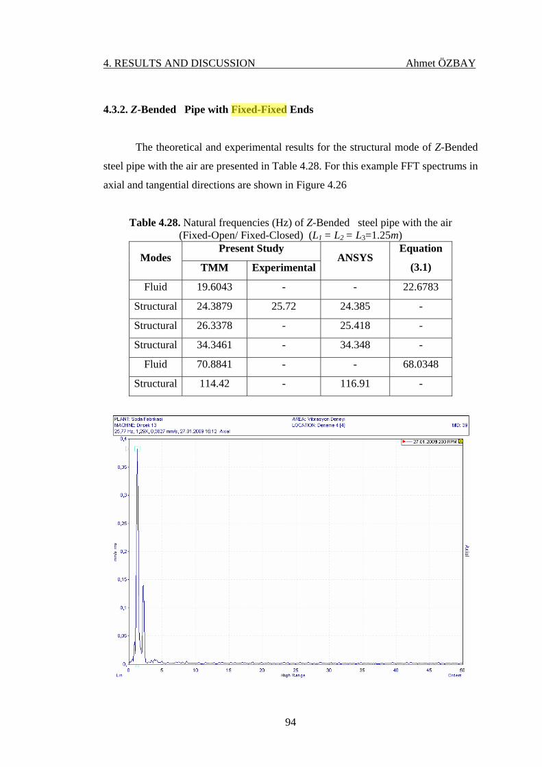
4. RESULTS AND DISCUSSION Ahmet ÖZBAY
94
4.3.2. Z-Bended Pipe with Fixed-Fixed Ends
The theoretical and experimental results for the structural mode of Z-Bended
steel pipe with the air are presented in Table 4.28. For this example FFT spectrums in
axial and tangential directions are shown in Figure 4.26
Table 4.28. Natural frequencies (Hz) of Z-Bended steel pipe with the air (Fixed-Open/ Fixed-Closed) (L1 = L2 = L3=1.25m)
Present Study Modes
TMM ExperimentalANSYS
Equation
(3.1)
Fluid 19.6043 - - 22.6783
Structural 24.3879 25.72 24.385 -
Structural 26.3378 - 25.418 -
Structural 34.3461 - 34.348 -
Fluid 70.8841 - - 68.0348
Structural 114.42 - 116.91 -
ITD
Highlight

4. RESULTS AND DISCUSSION Ahmet ÖZBAY
95
Figure 4.25. FFT Spectrums in axial and tangential directions of Z-Bended steel
pipe with the air (Fixed-Open/ Fixed-Closed) (L1 = L2 = L3=1.25m)
The theoretical and experimental results of Z-Bended steel pipe with the
water are presented in Table 4.29 . Figures 4.27 and 4.28 illustrate the experimental
pressure-time history of this pipe system at different external excitation frequencies
and when the external excitation frequency is equal to the fundamental liquid
frequency (94.12Hz). For the fundamental frequency in the structural mode, FFT
spectrums in tangential direction at two different locations are illustrated in Figure
4.29.

4. RESULTS AND DISCUSSION Ahmet ÖZBAY
96
Table 4.29. Natural frequencies (Hz) of Z-Bended steel pipe with the water (Fixed-Open/ Fixed-Closed) (L1 = L2 = L3=1.25m)
Present Study Modes
TMM ExperimentalANSYS
Equation
(3.1)
Structural 20.229 23.90 20.226 -
Structural 21.0474 - 21.082 -
Structural 28.5025 - 28.490 -
Fluid 95.1599 94.1176 - 93.7219
Structural 98.776 - 96.965 -
Structural 107.068 - 107.16 -
0
5
10
15
20
25
30
35
40
45
1 38 75 112 149 186 223 260 297 334 371 408 445 482 519 556
Time (s)
Pressure (Bar/10)
Figure 4.26. Experimental pressure-time history of Z-Bended steel pipe with the
water (Fixed-Open/ Fixed-Closed) (L1 = L2 = L3=1.25m) at different
external excitation frequencies.
ITD
Highlight
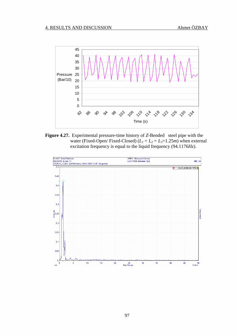
4. RESULTS AND DISCUSSION Ahmet ÖZBAY
97
05
1015202530354045
82 86 90 94 98 102
106
110
114
118
122
126
130
134
Time (s)
Pressure (Bar/10)
Figure 4.27. Experimental pressure-time history of Z-Bended steel pipe with the
water (Fixed-Open/ Fixed-Closed) (L1 = L2 = L3=1.25m) when external excitation frequency is equal to the liquid frequency (94.1176Hz).

4. RESULTS AND DISCUSSION Ahmet ÖZBAY
98
Figure 4.28. FFT Spectrums in tangential direction at two locations of Z-Bended
steel pipe with the water (Fixed-Open/ Fixed-Closed) (L1 = L2 = L3=1.25m)
The total length of the Z-Bended copper pipe system is considered as either
3m or 7m.
The theoretical and experimental results of Z-Bended copper pipe (L1 = L2 =
L3=1m) with the air are presented in Table 4.30 . For the fundamental frequency in
the structural mode (13.05Hz), FFT spectrums in both tangential and axial directions
are illustrated in Figure 4.30

4. RESULTS AND DISCUSSION Ahmet ÖZBAY
99
Table 4.30. Natural frequencies (Hz) of Z-Bended copper pipe with the air (Fixed-Open/ Fixed-Closed) (L1 = L2 = L3=1m)
Present Study Modes
TMM ExperimentalANSYS
Equation
(3.1)
Structural 11.2426 13.05 13.517 -
Structural 13.5169 - 14.200 -
Structural 18.9849 - 18.986 -
Fluid 30.4691 - - 28.3478
Structural 65.5427 - 65.934 -
Structural 72.2805 - 72.403 -
Fluid 89.3839 - - 85.0433
Structural 94.7097 - 93.895 -

4. RESULTS AND DISCUSSION Ahmet ÖZBAY
100
Figure 4.29. FFT spectrums in tangential and axial directions of Z-Bended copper
pipe with the air (Fixed-Open/ Fixed-Closed) (L1 = L2 = L3=1m)
The theoretical and experimental results of Z-Bended copper pipe (L1 = L2 =
L3=1m) with the water are presented in Table 4.31. For the fundamental frequency in
the structural mode (10.35Hz), FFT spectrums in both tangential and axial directions
are illustrated in Figure 4.31.

4. RESULTS AND DISCUSSION Ahmet ÖZBAY
101
Table 4.31. Natural Frequencies (Hz) of Z-Bended copper pipe with the water (Fixed-Open/ Fixed-Closed) (L1 = L2 = L3=1m)
Present Study Modes
TMM ExperimentalANSYS
Equation
(3.1)
Structural 10.2238 10.35 10.223 -
Structural 10.7357 - 10.740 -
Structural 14.3629 - 14.360 -
Structural 49.7901 - 49.869 -
Structural 54.7007 - 54.762 -
Structural 70.9215 - 71.018 -
Structural 71.6428 - 71.843 -
Structural 92.2388 - 94.131 -
Structural 94.9889 - 95.299 -
Fluid 117.056 - - 106.665
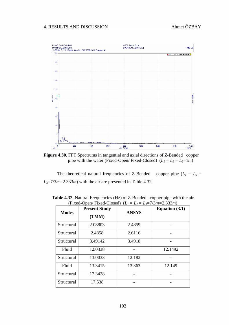
4. RESULTS AND DISCUSSION Ahmet ÖZBAY
102
Figure 4.30. FFT Spectrums in tangential and axial directions of Z-Bended copper
pipe with the water (Fixed-Open/ Fixed-Closed) (L1 = L2 = L3=1m)
The theoretical natural frequencies of Z-Bended copper pipe (L1 = L2 =
L3=7/3m=2.333m) with the air are presented in Table 4.32.
Table 4.32. Natural Frequencies (Hz) of Z-Bended copper pipe with the air (Fixed-Open/ Fixed-Closed) (L1 = L2 = L3=7/3m=2.333m)
Modes Present Study
(TMM) ANSYS
Equation (3.1)
Structural 2.08803 2.4859 -
Structural 2.4858 2.6116 -
Structural 3.49142 3.4918 -
Fluid 12.0338 - 12.1492
Structural 13.0033 12.182 -
Fluid 13.3415 13.363 12.149
Structural 17.3428 - -
Structural 17.538 - -

4. RESULTS AND DISCUSSION Ahmet ÖZBAY
103
The theoretical and experimental natural frequencies of Z-Bended copper
pipe (L1 = L2 = L3=7/3m=2.333m) with the water are presented in Table 4.33 .
Table 4.33. Natural Frequencies (Hz) of Z-Bended copper pipe with the water (Fixed-Open/ Fixed-Closed) (L1 = L2 = L3=7/3m=2.333m)
Present Study Modes
TMM ExperimentalANSYS
Equation
(3.1)
Structural 1.88015 - 1.8802 -
Structural 1.97513 - 1.9753 -
Structural 2.64087 - 2.6410 -
Structural 9.20088 - 9.2135 -
Structural 10.0919 - 10.107 -
Structural 13.1205 - 13.151 -
Structural 13.2652 - 13.302 -
Structural 17.3886 - 17.484 -
Structural 17.5729 - 17.640 -
Structural 32.2449 - 32.737 -
Fluid 44.8799 46.666 - 45.7141

4. RESULTS AND DISCUSSION Ahmet ÖZBAY
104
0
5
10
15
20
25
30
35
1 18 35 52 69 86 103 120 137 154 171 188 205 222 239 256
Time (s)
Pressure (Bar/10)
Figure 4.31. Experimental pressure-time history of Z-Bended copper pipe with the
water (Fixed-Open/ Fixed-Closed) (L1 = L2 = L3=7/3m=2.333m) at different external excitation frequencies.
0
5
10
15
20
25
30
35
33 35 37 39 41 43 45 47 49 51 53 55 57 59 61 63 65 67 69 71
Time (s)
Pressure (Bar/10)
Figure 4.32. Experimental pressure-time history of Z-Bended copper pipe with the
water (Fixed-Open/ Fixed-Closed) (L1 = L2 = L3=7/3m=2.333m) when external excitation frequency is equal to the liquid frequency (46.666 Hz).

4. RESULTS AND DISCUSSION Ahmet ÖZBAY
105
4.3.3. U-Bended Pipe with Fixed-Free Ends
In this case study, steel pipe is examined in a theoretical manner for both the
air and the water. Open-Closed fluid boundary conditions and fixed-free structural
end conditions are studied. The theoretical natural frequencies are listed in Table
4.34 for the air and in Table 4.35 for the water.
Table 4.34. Natural Frequencies (Hz) of U-Bended steel pipe with the air (Fixed-Open/ Free-Closed) (L1 = L2 = L3=1.25m)
Modes Present Study
(TMM) ANSYS
Equation (3.1)
Structural 6.61737 6.6171 -
Structural 6.69652 7.2448 -
Structural 11.1277 14.648 -
Structural 14.6476 15.057 -
Fluid 24.3281 - 22.6783
Structural 37.7906 37.7906 -
Table 4.35. Natural Frequencies (Hz) of U-Bended steel pipe with the water (Fixed-Open / Free-Closed) (L1 = L2 = L3=1.25m)
Modes Present Study
(TMM) ANSYS
Equation (3.1)
Structural 5.48901 5.4884 -
Structural 6.43686 6.0090 -
Structural 11.0398 12.149 -
Structural 12.1526 12.489 -
Structural 31.3657 31.345 -
Fluid 96.6866 - 94.9079
ITD
Highlight

4. RESULTS AND DISCUSSION Ahmet ÖZBAY
106
4.3.4. U-Bended Pipe with Fixed-Fixed Ends
Different lengths of pipes were connected as U Bended in this case. Open-
Closed fluid boundary conditions and fixed-fixed end conditions were applied to the
steel and copper pipes. Natural frequencies were found by transfer matrix method,
Ansys and experimentally and results listed in Tables.
Table 4.36. Natural Frequencies (Hz) of U-Bended steel pipe with the air (Fixed-Open / Fixed-Closed) (L1 = L2 = L3=1.25m)
Present Study Modes
TMM ExperimentalANSYS
Equation
(3.1)
Structural 18.5293 18.57 18.528 -
Fluid 15.0451 - - 22.6783
Structural 39.4704 - 29.548 -
Structural 40.6648 - 39.473 -
Fluid 71.8848 - - 68.0348
Structural 113.399 - 115.56 -
ITD
Highlight
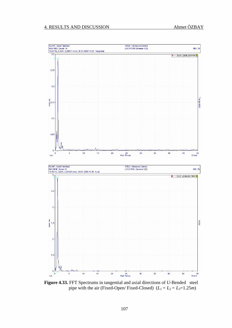
4. RESULTS AND DISCUSSION Ahmet ÖZBAY
107
Figure 4.33. FFT Spectrums in tangential and axial directions of U-Bended steel
pipe with the air (Fixed-Open/ Fixed-Closed) (L1 = L2 = L3=1.25m)

4. RESULTS AND DISCUSSION Ahmet ÖZBAY
108
Table 4.37. Natural Frequencies (Hz) of U-Bended steel pipe with the water (Fixed-Open / Fixed-Closed) (L1 = L2 = L3=1.25m)
Present Study Modes
TMM ExperimentalANSYS
Equation
(3.1)
Structural 15.3709 15.45 15.368 -
Structural 18.2968 - 24.508 -
Structural 32.7491 - 32.740 -
Structural 95.726 - 95.852 -
Structural 104.44 - 104.50 -
Fluid 119.597 - - 93.7219
Structural 152.141 - 152.62 -
Copper pipes were studied 3 m and 7m length again in this case.
Table 4.38. Natural Frequencies (Hz) of U-Bended cooper pipe with the air (Fixed-Open / Fixed-Closed) (L1 = L2 = L3=1m)
Present Study Modes
TMM ExperimentalANSYS
Equation
(3.1)
Structural 8.3232 10.95 10.340 -
Structural 10.3401 - 16.547 -
Structural 21.8065 - 21.809 -
Fluid 28.6991 - - 28.3478
Structural 65.0579 - 65.146 -
Structural 70.6204 - 70.735 -
Fluid 87.9053 - - 85.0433
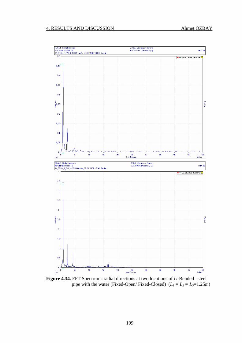
4. RESULTS AND DISCUSSION Ahmet ÖZBAY
109
Figure 4.34. FFT Spectrums radial directions at two locations of U-Bended steel
pipe with the water (Fixed-Open/ Fixed-Closed) (L1 = L2 = L3=1.25m)

4. RESULTS AND DISCUSSION Ahmet ÖZBAY
110
Figure 4.35. FFT Spectrums in radial and axial directions of U-Bended cooper pipe
with the air (Fixed-Open / Fixed-Closed) (L1 = L2 = L3=1m)

4. RESULTS AND DISCUSSION Ahmet ÖZBAY
111
Table 4.39. Natural Frequencies (Hz) of U-Bended cooper pipe with the water (Fixed-Open / Fixed-Closed) (L1 = L2 = L3=1m)
Present Study Modes
TMM ExperimentalANSYS
Equation
(3.1)
Structural 7.82132 8.05 7.8207 -
Structural 8.7379 - 12.516 -
Structural 16.4962 - 16.495 -
Structural 49.2127 - 49.274 -
Structural 53.4471 - 53.500 -
Structural 74.1259 - 78.320 -
Structural 78.0921 - 80.327 -
Structural 86.2918 - 86.648 -
Structural 89.6348 - 89.779 -
Fluid 109.275 - - 106.665
Table 4.40. Natural Frequencies (Hz) of U-Bended cooper pipe with the air (Fixed-Open / Fixed-Closed) (L1 = L2 = L3=2.333m)
Modes Present Study
(TMM) ANSYS Equation (3.1)
Structural 1.57107 1.9009 -
Structural 1.90083 3.0471 -
Structural 4.01121 4.0117 -
Fluid 12.0174 - 12.1492
Structural 13.0371 12.033 -
Structural 16.5752 13.057 -
Structural 16.581 19.150 -
Structural 19.0895 19.649 -

4. RESULTS AND DISCUSSION Ahmet ÖZBAY
112
Figure 4.36. FFT Spectrums in axial direction at two locations of U-Bended cooper
pipe with the water (Fixed-Open / Fixed-Closed) (L1 = L2 = L3=1m)

4. RESULTS AND DISCUSSION Ahmet ÖZBAY
113
Table 4.41. Natural Frequencies (Hz) of U-Bended cooper pipe with the air (Fixed-Open / Fixed-Closed) (L1 = L2 = L3=2.333m)
Present Study Modes
TMM ExperimentalANSYS
Equation
(3.1)
Structural 1.43772 - 1.4377 -
Structural 1.6113 - 2.3047 -
Structural 3.03398 - 3.0343 -
Structural 9.08962 - 9.1015 -
Structural 9.86178 - 9.8760 -
Structural 13.9154 - 14.484 -
Structural 14.4396 - 14.862 -
Structural 16.0525 - 16.118 -
Structural 16.5912 - 16.642 -
Structural 32.2892 - 32.882 -
Fluid 46.0184 46,6233 - 45.7141
In Figures 4.37 and 4.38, the gauge pressure and excitation frequencies are
plotted vs. time. It is also observed from these figures that the pressure react the
excitation frequency near the liquid natural frequency.

4. RESULTS AND DISCUSSION Ahmet ÖZBAY
114
0
5
10
15
20
25
30
35
1 40 79 118 157 196 235 274 313 352 391 430 469 508 547 586
Time (s)
Pressure (Bar/10)
Figure 4.37. Experimental pressure-time history of U-Bended copper pipe with the
water (Fixed-Open/ Fixed-Closed) (L1 = L2 = L3=2.333m) at different external excitation frequencies.
0
5
10
15
20
25
30
35
267
271
275
279
283
287
291
295
299
303
307
311
315
319
Time (s)
Pressure (Bar/10)
Figure 4.38. Experimental pressure-time history of U-Bended copper pipe with the water (Fixed-Open/ Fixed-Closed) (L1 = L2 = L3=2.333m) when external excitation frequency is equal to the liquid frequency (46,623Hz).

4. RESULTS AND DISCUSSION Ahmet ÖZBAY
115
4.4. Three Pipes in Two Planes
The pipe configuration considered in this section is shown in Figure 4.39.
For simplicity the length of each pipe is assumed to be equal in the following case
studies.
Figure 4.39. 3D-Bended pipe supported at two ends
4.4.1. 3D-Bended Pipe with Fixed-Free Ends
In this case study for 3-D pipe configuration, the pipe material is determined
as the steel. The length of each pipe is assumed to be equal (L1 = L2 = L3=1.25m).
Both the air and the water are used as the fluids. Closed-closed fluid boundary
conditions and fixed-free structural end conditions are handled. The theoretical
results for the air are presented in Table 4.42 and for the water are presented in Table
4.43.
1.25m
1.25m
1.25m
ITD
Highlight
ITD
Highlight

4. RESULTS AND DISCUSSION Ahmet ÖZBAY
116
Table 4.42. Natural Frequencies (Hz) of 3D-Bended steel pipe with the air (Fixed-Open / Free-Closed) (L1 = L2 = L3=1.25m)
Modes Present Study
(TMM) ANSYS Equation (3.1)
Structural 5.07353 5.8365 -
Structural 6.31677 6.4474 -
Structural 14.5468 16.121 -
Structural 17.5303 17.610 -
Fluid 26.0289 - 22.6783
Structural 32.1722 32.370 -
Structural 45.5397 47.326 -
Fluid 74.0333 - 68.0348
Fluid 116.818 - 113.391
Structural 132.501 132.69 -
Table 4.43. Natural Frequencies (Hz) of 3D-Bended steel pipe with the water (Fixed-Open / Free-Closed) (L1 = L2 = L3=1.25m)
Modes Present Study
(TMM) ANSYS
Equation (3.1)
Structural 4.84057 4.8409
Structural 5.34791 5.3476
Structural 13.3656 13.371
Structural 14.6104 14.606
Structural 26.8324 26.848
Structural 39.2388 39.253
Fluid 103.785 - 94.9079
Structural 110.3 110.05

4. RESULTS AND DISCUSSION Ahmet ÖZBAY
117
4.4.2. 3D-Bended Pipe with Fixed-Fixed Ends
The theoretical and experimental results in the fundamental structural mode
of 3D-Bended steel pipe with the air are presented in Table 4.44. For this example
FFT spectrums in tangential direction are shown in Figure 4.40.
Table 4.44. Natural Frequencies (Hz) of 3D-Bended steel pipe with the air (Fixed-Open / Fixed-Closed) (L1 = L2 = L3=1.25m)
Present Study Modes
TMM ExperimentalANSYS Equation (3.1)
Structural 17.9003 20.10 20.699 -
Fluid 24.1988 - - 22.6783
Structural 33.8281 - 34.563 -
Structural 34.5657 - 34.839 -
Fluid 70.9162 - - 68.0348
Fluid 115.91 - - 113.391
Structural 122.079 - 122.09 -
Structural 122.249 - 122.30 -
Structural 174.064 - 174.72 -
ITD
Highlight
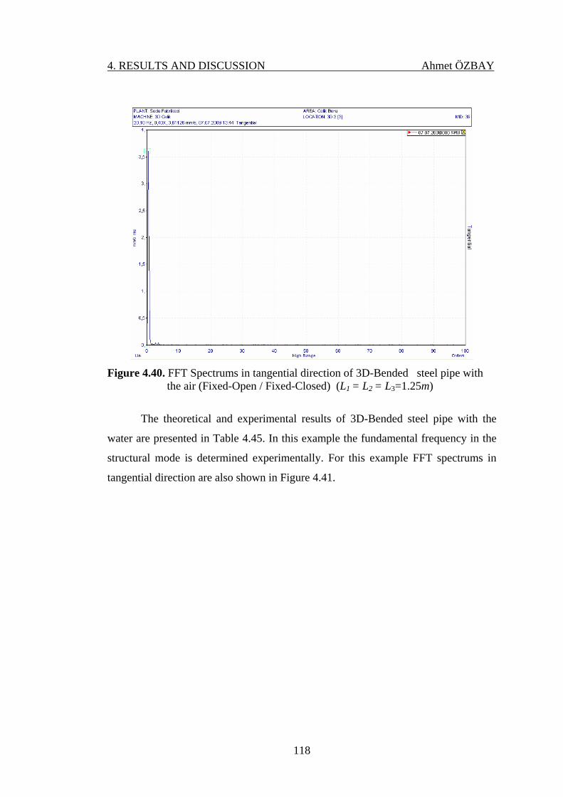
4. RESULTS AND DISCUSSION Ahmet ÖZBAY
118
Figure 4.40. FFT Spectrums in tangential direction of 3D-Bended steel pipe with
the air (Fixed-Open / Fixed-Closed) (L1 = L2 = L3=1.25m)
The theoretical and experimental results of 3D-Bended steel pipe with the
water are presented in Table 4.45. In this example the fundamental frequency in the
structural mode is determined experimentally. For this example FFT spectrums in
tangential direction are also shown in Figure 4.41.
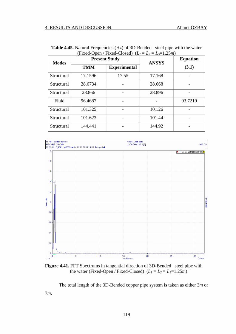
4. RESULTS AND DISCUSSION Ahmet ÖZBAY
119
Table 4.45. Natural Frequencies (Hz) of 3D-Bended steel pipe with the water (Fixed-Open / Fixed-Closed) (L1 = L2 = L3=1.25m)
Present Study Modes
TMM Experimental ANSYS
Equation
(3.1)
Structural 17.1596 17.55 17.168 -
Structural 28.6734 - 28.668 -
Structural 28.866 - 28.896 -
Fluid 96.4687 - - 93.7219
Structural 101.325 - 101.26 -
Structural 101.623 - 101.44 -
Structural 144.441 - 144.92 -
Figure 4.41. FFT Spectrums in tangential direction of 3D-Bended steel pipe with
the water (Fixed-Open / Fixed-Closed) (L1 = L2 = L3=1.25m)
The total length of the 3D-Bended copper pipe system is taken as either 3m or
7m.

4. RESULTS AND DISCUSSION Ahmet ÖZBAY
120
The theoretical and experimental results of 3D-Bended copper pipe (L1 = L2 =
L3=1m) with the air are presented in Table 4.46. For the fundamental frequency in
the structural mode (10.71Hz), FFT spectrums in the axial direction are illustrated in
Figure 4.42.
Table 4.46. Natural Frequencies (Hz) of 3D-Bended copper pipe with the air
(Fixed-Open / Fixed-Closed) (L1 = L2 = L3=1m) Present Study
Modes TMM Experimental
ANSYS Equation
(3.1)
Structural 9.86233 10.71 11.541 -
Structural 18.0117 - 19.207 -
Structural 19.2065 - 19.456 -
Fluid 30.5497 - - 28.3478
Structural 68.3461 - 68.644 -
Structural 68.6145 - 68.719 -
Fluid 88.2313 - - 85.0433
Structural 98.4998 - 98.815 -
Structural 99.065 - 99.026 -

4. RESULTS AND DISCUSSION Ahmet ÖZBAY
121
Figure 4.42. FFT Spectrums in tangential direction of 3D-Bended copper pipe with
the air (Fixed-Open / Fixed-Closed) (L1 = L2 = L3=1m)
The theoretical and experimental results of 3D-Bended copper pipe (L1 = L2 =
L3=1m) with the water are presented in Table 4.47. For the fundamental frequency in
the structural mode (7.65Hz), FFT spectrums in the radial direction are illustrated in
Figure 4.43.

4. RESULTS AND DISCUSSION Ahmet ÖZBAY
122
Table 4.47. Natural Frequencies (Hz) of 3D-Bended copper pipe with the water (Fixed-Open / Fixed-Closed) (L1 = L2 = L3=1m)
Present Study Modes
TMM ExperimentalANSYS
Equation
(3.1)
Structural 8.72818 7.65 8.7290 -
Structural 14.5278 - 14.527 -
Structural 14.7123 - 14.716 -
Structural 51.8515 - 51.919 -
Structural 51.9149 - 51.976 -
Structural 74.4193 - 74.739 -
Structural 74.6579 - 74.739 -
Fluid 116.289 - - 106.665
Figure 4.43. FFT Spectrums in radial direction of 3D-Bended copper pipe with the
water (Fixed-Open / Fixed-Closed) (L1 = L2 = L3=1m)
The theoretical natural frequencies of 3D-Bended copper pipe (L1 = L2 =
L3=7/3m=2.333m) with the air are presented in Table 4.48.

4. RESULTS AND DISCUSSION Ahmet ÖZBAY
123
Table 4.48. Natural Frequencies (Hz) of 3D-Bended copper pipe with the air (Fixed-Open / Fixed-Closed) (L1 = L2 = L3=2.333m)
Modes Present Study
(TMM) ANSYS Equation (3.1)
Structural 1.82348 2.1218 -
Structural 3.33919 3.5341 -
Structural 3.53379 3.5809 -
Fluid 12.5046 - 12.1492
Structural 12.6687 12.675 -
Structural 13.0027 12.687 -
Structural 18.2772 18.295 -
The theoretical and experimental natural frequencies of 3D-Bended copper
pipe (L1 = L2 = L3=7/3m=2.333m) with the water are presented in Table 4.49. In this
example, the fundamental frequency in the fluid mode is measured experimentally.
Figures 4.44 and 4.45 illustrate the experimental pressure-time history of this pipe
system at different external excitation frequencies and when the external excitation
frequency is equal to the fundamental liquid frequency (47.806Hz).

4. RESULTS AND DISCUSSION Ahmet ÖZBAY
124
Table 4.49. Natural Frequencies (Hz) of 3D-Bended copper pipe with the water (Fixed-Open / Fixed-Closed) (L1 = L2 = L3=2.333m)
Present Study Modes
TMM Experimental ANSYS
Equation
(3.1)
Structural 1.60477 - 1.6050 -
Structural 2.67282 - 2.6733 -
Structural 2.7081 - 2.7086 -
Structural 9.57339 - 9.5875 -
Structural 9.58258 - 9.5966 -
Structural 13.7737 - 13.839 -
Structural 13.8412 - 13.866 -
Structural 16.7317 - 16.917 -
Structural 17.0937 - 17.141 -
Structural 32.7067 - 33.223 -
Fluid 43.6206 47.806 - 45.7141
-10
-5
0
5
10
15
20
25
30
35
40
1 44 87 130 173 216 259 302 345 388 431 474 517 560 603 646 689 732 775 818 861 904 947
Time (s)
Pressure (Bar/100)
Figure 4.44. Experimental pressure-time history of 3D-Bended copper pipe with the
water (Fixed-Open/ Fixed-Closed) (L1 = L2 = L3=2.333m) at different external excitation frequencies.

4. RESULTS AND DISCUSSION Ahmet ÖZBAY
125
-10
-5
0
5
10
15
20
25
30
35
40
403
408
413
418
423
428
433
438
443
448
453
458
463
468
473
478
483
488
493
498
503
508
Time (s)
Pressure (Bar/10)
Figure 4.45. Experimental pressure-time history of 3D-Bended copper pipe with the
water (Fixed-Open/ Fixed-Closed) (L1 = L2 = L3=2.333m) when external excitation frequency is equal to the liquid frequency (47.8 Hz).
4.5. Pipes on Elastic Foundation
In this section the effect of the elastic foundation (Figure 4.46) on the natural
frequencies of the pipe system with free ends is worked out with the help of the
transfer matrix method. The pipe is rested on the elastic foundation along z-direction
as shown in Figure 4.46.
Figure 4.46. Free ended pipe on elastic foundation
l
Δ
kf
X
Y
Z
ITD
Highlight

4. RESULTS AND DISCUSSION Ahmet ÖZBAY
126
The natural frequencies in structural modes of such single-spanned isotropic
beams with hollow section are given in an analytical manner by the followings
formulas (Pestel and Leckie, 1963).
p
y
ny
nn A
EI
EIl
l ρλπλ
ω21
4
4
2
2
12 ⎟
⎟⎠
⎞⎜⎜⎝
⎛ Φ+= (4.1.)
Δ=Φ /fk (4.2.)
πλ ⎟⎠⎞
⎜⎝⎛ +=
21nn (4.3.)
where ρ represents mass density of pipe, kf is foundation stiffness, Ap Cross-sectional
area, Iy Moment of inertia and Φ is the foundation modulus.
In this part of this study single-spanned , L-Bended and 3D-Bended pipes
rested on an elastic foundation with free ends are examined.
4.5.1. Free Ended Single -Spanned Pipe on an Elastic Foundation
The 6m-length steel and copper single-spanned pipes with free ends are
handled here. Both the air and water are used as fluids. The frequencies in structural
modes obtained by the transfer matrix approach are compared with the exact
frequencies evaluated by Equation (4.1). The results are listed in Tables 4.50-4.53.
It is observed from those tables that the transfer matrix method gives quite
reasonable results.

4. RESULTS AND DISCUSSION Ahmet ÖZBAY
127
Table 4.50. Natural Frequencies (Hz) of 6m length free ended steel pipe with the air
on elastic foundation (kf = 100000 N/m3, Δ = 1m) (Free-Open/ Free-Closed)
Modes Present Study
(TMM) Theoretical Equation (3.1)
Structural 11.5036 11.5026 -
Fluid 14.1798 - 14.1739
Structural 25.8147 25.9200 -
Fluid 42.5237 - 42.5217
Structural 49.0373 49.3283 -
Fluid 70.8706 - 70.8695
Structural 80.2735 80.9887 -
Fluid 99.2181 - 99.2173
Structural 119.009 120.7183 -
Fluid 127.566 - 127.5652
Structural 155.913 155.9130 -
Table 4.51. Natural Frequencies (Hz) of 6m length free ended steel pipe with the
water on elastic foundation (kf = 100000 N/m3, Δ = 1m) (Free-Open/ Free-Closed)
Modes Present Study
(TMM) Theoretical
Equation (3.1)
Structural 9.54148 9.5379 -
Structural 21.4124 21.4929 -
Structural 40.6767 40.9030 -
Fluid 58.9688 - 58.5762
Structural 66.5919 67.1558 -
Structural 98.9105 100.0996 -
Structural 137.462 139.687 -

4. RESULTS AND DISCUSSION Ahmet ÖZBAY
128
Table 4.52. Natural Frequencies (Hz) of 6m length free ended copper pipe with the
air on elastic foundation (kf = 100000 N/m3, Δ = 1m) (Free-Open/ Free-Closed)
Modes Present Study
(TMM) Theoretical
Equation (3.1)
Fluid 14.1998 - 14.1738
Structural 18.9776 19.1708 -
Structural 20.698 20.8824 -
Structural 25.526 25.6883 -
Structural 34.2529 34.4112 -
Fluid 42.5302 - 42.5216
Structural 46.7354 - -
Structural 62.6181 62.9014 -
Fluid 70.8733 - 70.869
Structural 81.6408 82.0799 -
Fluid 99.2195 - 99.2172
Structural 103.643 104.3201 -
Fluid 128.523 - 127.5649
Fluid 155.881 - 155.9127
Structural 156.586 157.6894 -

4. RESULTS AND DISCUSSION Ahmet ÖZBAY
129
Table 4.53. Natural Frequencies (Hz) of 6m length free ended copper pipe with the
water on elastic foundation (kf = 100000 N/m3, Δ = 1m) (Free-Open/ Free-Closed)
Modes Present Study
(TMM) Theoretical
Equation (3.1)
Structural 14.3538 14.4999 -
Structural 15.6552 15.7944 -
Structural 19.3072 19.4294 -
Structural 25.9085 26.0270 -
Structural 35.3512 35.4953 -
Structural 47.3665 47.5757 -
Fluid 54.7762 - 53.3323
Structural 61.7582 62.0814 -
Structural 78.4048 78.9028 -
Structural 97.2265 97.9775 -
Structural 118.06 119.2688 -
Structural 143.247 142.7546 -
Fluid 159.888 - 159.996
Above, the results show that, transfer matrix method gives quite reasonable
results when compared with theoretical ones for free ended single-spanned pipe on
an elastic foundation.
4.5.2. L-Bended Free Ended Pipe on an Elastic Foundation
This example is studied here at the first time (Figure 4.47). The total length of
the pipe system made of either steel or copper is 3m. (L1 = L2 = 1.5m). The
theoretical results of TMM are listed in Tables 4.54- 4.57.

4. RESULTS AND DISCUSSION Ahmet ÖZBAY
130
Figure 4.47. L-Bended pipe on elastic foundation
Table 4.54. Natural Frequencies (Hz) of 3m length L-Bended free ended steel pipe with the air on elastic foundation (kf = 100000 N/m3, Δ = 0.5m)
(Free-Open/ Free-Closed) (L1 = L2 = 1.5m)
Modes Present Study
(TMM) Equation (3.1)
Fluid 14.1748 14.1739
Structural 23.5469 -
Structural 33.543 -
Structural 34.4259 -
Fluid 42.3477 42.5217
Structural 43.823 -
Af 70.7304 70.8695
Structural 82.9094 -
Structural 84.0941 -
Af 98.9495 99.2173
Structural 103.008 -

4. RESULTS AND DISCUSSION Ahmet ÖZBAY
131
Table 4.55. Natural Frequencies (Hz) of 3m length L-Bended free ended steel pipe with the water on elastic foundation (kf = 100000 N/m3, Δ = 0.5m)
(Free-Open/ Free-Closed) (L1 = L2 = 1.5m)
Modes Present Study
(TMM)
Equation (3.1)
Structural 8.08359 -
Structural 21.3995 -
Structural 22.3519 -
Structural 30.3128 -
Structural 31.7264 -
Fluid 58.6578 58.5762
Structural 66.4431 -
Structural 67.4916
Table 4.56. Natural Frequencies (Hz) of 3m length L-Bended free ended copper pipe with the air on elastic foundation (kf = 100000 N/m3, Δ = 0.5m)
(Free-Open/ Free-Closed) (L1 = L2 = 1.5m)
Modes Present Study
(TMM)
Equation (3.1)
Fluid 14.1918 14.1738
Structural 18.8498 -
Structural 20.6975 -
Structural 23.012 -
Structural 34.2405 -
Structural 34.5786
Structural 39.9821 -
Structural 40.7105 -
Fluid 42.4084 42.5216
Structural 62.5554 -
Structural 62.9645 -
Fluid 70.3662 70.8694

4. RESULTS AND DISCUSSION Ahmet ÖZBAY
132
Table 4.57. Natural Frequencies (Hz) of 3m length L-Bended free ended copper pipe with the water on elastic foundation (kf = 100000 N/m3, Δ = 0.5m)
(Free-Open/ Free-Closed) (L1 = L2 = 1.5m)
Modes Present Study
(TMM)
Equation (3.1)
Structural 14.2573 -
Structural 15.7879 -
Structural 17.4076 -
Structural 25.8992 -
Structural 26.1584 -
Structural 30.8035 -
Structural 47.3187 -
Fluid 53.9701 53.3323
Structural 54.8135 -
4.5.3. 3D-Bended Free Ended Pipe on an Elastic Foundation
This example is also studied here at the first time (Figure 4.48). The total
length of the pipe system made of either steel or copper is 3.75m. (L1 = L2 =L3=
1.25m). The theoretical results of TMM are listed in Tables 4.58- 4.61.

4. RESULTS AND DISCUSSION Ahmet ÖZBAY
133
Figure 4.48. 3D-bended pipe on elastic foundation
Table 4.58. Natural Frequencies (Hz) of 3m length 3D-Bended free ended steel pipe with the air on elastic foundation (kf = 100000 N/m3, Δ = 1.25m)
(Free-Open/ Free-Closed) (L1 = L2 = 1.25m)
Modes Present Study
(TMM) Equation (3.1)
Fluid 20.5961 22.6783
Structural 27.0431 -
Structural 39.4607 -
Structural 41.2942 -
Fluid 71.0473 68.0348
Fluid 116.107 113.391

4. RESULTS AND DISCUSSION Ahmet ÖZBAY
134
Table 4.59. Natural Frequencies (Hz) of 3m length 3D-Bended free ended steel pipe with the water on elastic foundation kf = 100000 N/m3, Δ = 1.25m)
(Free-Open/ Free-Closed) (L1 = L2 = 1.25m)
Modes Present Study
(TMM)
Equation (3.1)
Structural 17.7897 -
Structural 29.2794 -
Fluid 96.4906 93.7219
Structural 101.497 -
Table 4.60. Natural Frequencies (Hz) of 3m length 3D-Bended free ended copper pipe with the air on elastic foundation kf = 100000 N/m3, Δ = 1.25m)
(Free-Open/ Free-Closed) (L1 = L2 = 1.25m)
Modes Present Study
(TMM) Equation (3.1)
Structural 11.6188 -
Structural 21.5722 -
Fluid 22.385 22.6782
Structural 24.6739 -
Structural 47.6588 -
Fluid 65.9793 68.0347

4. RESULTS AND DISCUSSION Ahmet ÖZBAY
135
Table 4.61. Natural Frequencies (Hz) of 3m length 3D-Bended free ended copper pipe with the water on elastic foundation kf = 100000 N/m3, Δ = 1.25m)
(Free-Open/ Free-Closed) (L1 = L2 = 1.25m)
Modes Present Study
(TMM)
Equation (3.1)
Structural 11.1591 -
Structural 16.4594 -
Structural 36.1211 -
Structural 49.8572 -
Structural 60.2237 -
Fluid 86.7394 85.3317
4.6. Parametric Studies
In this part of the present work, a parametric study is carried out to
understand correctly the vibrational behavior of the piping systems filled by either
the water or the air. 2” nominal diameter-steel and 1” nominal diameter-copper
pipes are studied. Either fixed-fixed or fixed-free structural boundary conditions are
considered with closed-closed fluid boundary conditions. The first four structural and
fluid natural frequencies are used to draw the diagrams which show the variation of
the natural frequencies with either the slenderness ratio, L/d, or the bend angleα .
4.6.1. Effect of the Slenderness Ratio on the Natural Frequencies
Here single-spanned pipe system is considered. Variation of the natural
frequencies of a single-spanned steel/copper pipe filled by the air/water with the
slenderness ratio for different boundary conditions are illustrated in Figures 4.49-
4.56. The theoretical results are also presented in Tables 4.62-4.65.
As guessed, increasing the slenderness ratio, L/d, decreases the natural
frequencies in both the structural and fluid modes. The fundamental frequency in the
fluid mode increases with the density of the fluid.
ITD
Highlight

4. RESULTS AND DISCUSSION Ahmet ÖZBAY
136
Table 4.62. Variation of the natural frequencies in Hz of a single-spanned steel pipe with the slenderness ratio (Fixed-Fixed and Open-Closed)
Natural frequencies
Structural modes Fluid modes
Filled
by
L/d 1ω 2ω 3ω 4ω 1ω 2ω 3ω 4ω
1 121.300 169.938 235.516 271.901 1410 4231 7052 9872 2 57.609 84.969 111.979 169.938 705 2116 3526 4936 4 35.625 56.646 71.125 90.633 470 1410 2351 3291 6 24.447 42.485 50.596 67.975 353 1058 1763 2468 8 17.789 33.988 38.202 54.380 282 846 1410 1974 10 13.474 28.323 29.938 45.317 235 705 1175 1645 15 10.520 24.084 24.277 38.843 201 604 1007 1410
Air
20 8.417 19.766 21.242 33.443 176 529 881 1234 1 100625 169938 197159 271901 5902 17707 29511 41316
2 47807 84969 93576 135951 2951 8853 14756 20658
4 29574 56646 59303 90634 1967 5902 9837 13772
6 20298 42134 42484 67489 1476 4427 7378 10329
8 14771 31792 33988 51549 1180 3541 5902 8263
10 11188 24905 28323 40954 984 2951 4919 6886
15 8735 20029 24277 33429 843 2530 4216 5902
Water
20 6987 16434 21242 27834 738 2213 3689 5164

4. RESULTS AND DISCUSSION Ahmet ÖZBAY
137
Table 4.63. Variation of the natural frequencies in Hz of a single-spanned copper pipe with the slenderness ratio (Fixed-Fixed and Open-Closed)
Natural frequencies
Structural modes Fluid modes
Filled
by
L/d
1ω 2ω 3ω 4ω 1ω 2ω 3ω 4ω
1 167.254 232.730 325.856 382.415 3037 9112 15186 21261
2 79.766 116.365 155.108 191.207 1519 4556 7593 10630
4 49.592 77.577 98.695 127.472 1012 3037 5062 7087
6 34.215 58.182 70.404 95.603 759 2278 3797 5315
8 25.018 46.546 53.330 76.483 607 1822 3037 4252
10 19.026 38.788 41.931 63.736 506 1519 2531 3543
15 14.904 33.247 33.837 54.631 434 1302 2169 3037
Air
20 11.956 27.849 29.091 46.891 380 1139 1898 2658
1 126.526 232.730 248.908 361.059 30425 91274 152123 212972
2 60.367 116.365 185.361 216.683 15212 45637 76062 106486
4 37.547 75.148 77.576 118.974 10142 30425 50708 70991
6 25.912 53.526 58.183 85.571 7606 22818 38031 53243
8 18.949 40.510 46.546 65.513 6085 18255 30425 42594
10 14.410 31.835 38.788 52.171 5071 15212 25354 35495
15 11.288 25.681 33.247 42.685 4346 13039 21732 30425
Water
20 9.054 21.130 29.091 35.622 3803 11409 19015 26621
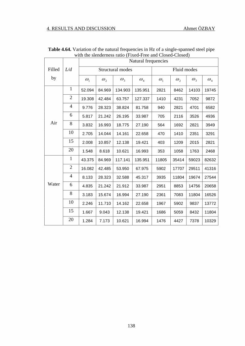
4. RESULTS AND DISCUSSION Ahmet ÖZBAY
138
Table 4.64. Variation of the natural frequencies in Hz of a single-spanned steel pipe with the slenderness ratio (Fixed-Free and Closed-Closed)
Natural frequencies
Structural modes Fluid modes
Filled
by
L/d
1ω 2ω 3ω 4ω 1ω 2ω 3ω 4ω
1 52.094 84.969 134.903 135.951 2821 8462 14103 19745
2 19.308 42.484 63.757 127.337 1410 4231 7052 9872
4 9.776 28.323 38.824 81.758 940 2821 4701 6582
6 5.817 21.242 26.195 33.987 705 2116 3526 4936
8 3.832 16.993 18.775 27.190 564 1692 2821 3949
10 2.705 14.044 14.161 22.658 470 1410 2351 3291
15 2.008 10.857 12.138 19.421 403 1209 2015 2821
Air
20 1.548 8.618 10.621 16.993 353 1058 1763 2468
1 43.375 84.969 117.141 135.951 11805 35414 59023 82632
2 16.082 42.485 53.950 67.975 5902 17707 29511 41316
4 8.133 28.323 32.588 45.317 3935 11804 19674 27544
6 4.835 21.242 21.912 33.987 2951 8853 14756 20658
8 3.183 15.674 16.994 27.190 2361 7083 11804 16526
10 2.246 11.710 14.162 22.658 1967 5902 9837 13772
15 1.667 9.043 12.138 19.421 1686 5059 8432 11804
Water
20 1.284 7.173 10.621 16.994 1476 4427 7378 10329

4. RESULTS AND DISCUSSION Ahmet ÖZBAY
139
Table 4.65. Variation of the natural frequencies in Hz of a single-spanned copper pipe with the slenderness ratio (Fixed-Free and Closed-Closed)
Natural frequencies
Structural modes Fluid modes
Filled
by
L/d 1ω 2ω 3ω 4ω 1ω 2ω 3ω 4ω
1 72.668 116.365 188.084 191.207 6075 18224 30373 42522
2 27.314 58.183 88.809 95.604 3037 9112 15186 21261
4 13.932 38.788 54.319 63.736 2025 6075 10124 14174
6 8.322 29.091 36.838 47.802 1519 4556 7593 10630
8 5.493 23.273 26.523 38.242 1215 3645 6075 8504
10 3.883 19.394 19.913 31.868 1012 3037 5062 7087
15 2.884 15.438 16.624 27.315 868 2603 4339 6075
Air
20 2.225 12.281 14.545 23.901 759 2278 3797 5315
1 55.217 150.979 191.207 236.240 60849 182547 304246 425944
2 20.770 58.183 68.972 95.604 30425 91274 152123 212972
4 10.579 38.788 41.738 63.736 20283 60849 101415 141981
6 6.312 28.177 29.091 47.802 15212 45637 76062 106486
8 4.163 20.235 23.273 38.242 12170 36509 60849 85189
10 2.941 15.166 19.394 31.868 10142 30425 50708 70991
15 2.184 11.743 16.624 27.315 8693 26078 43464 60849
Water
20 1.684 9.333 14.546 22.657 7606 22818 38031 53243

4. RESULTS AND DISCUSSION Ahmet ÖZBAY
140
0,0E+00
5,0E+04
1,0E+05
1,5E+05
2,0E+05
2,5E+05
3,0E+05
1 2 3 4 5 6 7 8 9 10 11 12 13 14 15 16 17 18 19 20 21 22
L/d
ω s (Hz)
ωs1
ωs2
ωs3
ωs4
(a)
0
2000
4000
6000
8000
10000
12000
1 3 5 7 9 11 13 15 17 19 21 23 25
L/d
wf
wf1wf2wf3wf4
(b)
Figure 4.49. Variation of the natural frequencies of a single-spanned steel pipe filled
by the air with the slenderness ratio (Fixed-Fixed and Open-Closed) a) Structural Modes b) Fluid Modes

4. RESULTS AND DISCUSSION Ahmet ÖZBAY
141
0,0E+00
5,0E+04
1,0E+05
1,5E+05
2,0E+05
2,5E+05
3,0E+05
1 2 3 4 5 6 7 8 9 10 11 12 13 14 15 16 17 18 19 20 21 22 23 24 25L/d
ω s (Hz)
ωs1
ωs2
ωs3
ωs4
(a)
05000
1000015000200002500030000350004000045000
1 3 5 7 9 11 13 15 17 19 21 23 25
L/d
wf (Hz)
(b)
Figure 4.50. Variation of the natural frequencies of a single-spanned steel pipe filled by the water with the slenderness ratio (Fixed-Fixed and Open-Closed) a) Structural Modes b) Fluid Modes

4. RESULTS AND DISCUSSION Ahmet ÖZBAY
142
0,0E+00
2,0E+04
4,0E+04
6,0E+04
8,0E+04
1,0E+05
1,2E+05
1,4E+05
1,6E+05
1 2 3 4 5 6 7 8 9 10 11 12 13 14 15 16 17 18 19 20 21 22 23 24 25L/d
ω s(Hz)
ωs1ωs2ωs4ωs4
(a)
0
5000
10000
15000
20000
25000
1 3 5 7 9 11 13 15 17 19 21 23 25L/d
ωf (Hz)
ωf1ωf2ωf3ωf4
(b)
Figure 4.51. Variation of the natural frequencies of a single-spanned steel pipe filled by the air with the slenderness ratio (Fixed-Free and Closed-Closed) a) Structural Modes b) Fluid Modes

4. RESULTS AND DISCUSSION Ahmet ÖZBAY
143
0,0E+00
2,0E+04
4,0E+04
6,0E+04
8,0E+04
1,0E+05
1,2E+05
1,4E+05
1,6E+05
1 2 3 4 5 6 7 8 9 10 11 12 13 14 15 16 17 18 19 20 21 22 23 24 25L/d
ω s(Hz)
ωs1
ωs2
ωs3
ωs4
(a)
0
10000
20000
30000
40000
50000
60000
70000
80000
90000
1 3 5 7 9 11 13 15 17 19 21 23 25
L/d
ωf (Hz)
ωf1ωf2ωf3ωf4
(b)
Figure 4.52. Variation of the natural frequencies of a single-spanned steel pipe filled by the water with the slenderness ratio (Fixed-Free and Closed-Closed) a) Structural Modes b) Fluid Modes

4. RESULTS AND DISCUSSION Ahmet ÖZBAY
144
0,0E+00
5,0E+04
1,0E+05
1,5E+05
2,0E+05
2,5E+05
3,0E+05
3,5E+05
4,0E+05
4,5E+05
1 3 5 7 9 11 13 15 17 19 21 23 25
L/d
ω s (Hz)
ωs1
ωs2
ωs3
ωs4
(a)
0
5000
10000
15000
20000
25000
1 3 5 7 9 11 13 15 17 19 21 23 25
L/d
ωf (Hz)
ωf1ωf2ωf3ωf4
(b)
Figure 4.53. Variation of the natural frequencies of a single-spanned copper pipe filled by the air with the slenderness ratio (Fixed-Fixed and Open-Closed) a) Structural Modes b) Fluid Modes

4. RESULTS AND DISCUSSION Ahmet ÖZBAY
145
0,0E+00
5,0E+04
1,0E+05
1,5E+05
2,0E+05
2,5E+05
3,0E+05
3,5E+05
4,0E+05
1 3 5 7 9 11 13 15 17 19 21 23 25L/d
s (Hz) ωs1ωs2ωs3ωs4
(a)
0
50000
100000
150000
200000
250000
1 3 5 7 9 11 13 15 17 19 21 23 25
L/d
ω f (Hz)
ωf1ωf2ωf3ωf4
(b)
Figure 4.54. Variation of the natural frequencies of a single-spanned copper pipe filled by the water with the slenderness ratio (Fixed-Fixed and Open-Closed) a) Structural Modes b) Fluid Modes

4. RESULTS AND DISCUSSION Ahmet ÖZBAY
146
0,0E+00
5,0E+04
1,0E+05
1,5E+05
2,0E+05
2,5E+05
1 2 3 4 5 6 7 8 9 10 11 12 13 14 15 16 17 18 19 20 21 22 23 24 25L/d
ω s(Hz )
ωs1
ωs2
ωs3
ωs4
(a)
0
5000
10000
15000
20000
25000
30000
35000
40000
45000
1 3 5 7 9 11 13 15 17 19 21 23 25
L/d
ωf (Hz)
ωf1ωf2ωf3ωf4
(b)
Figure 4.55. Variation of the natural frequencies of a single-spanned copper pipe
filled by the air with the slenderness ratio (Fixed-Free and Closed-Closed) a) Structural Modes b) Fluid Modes
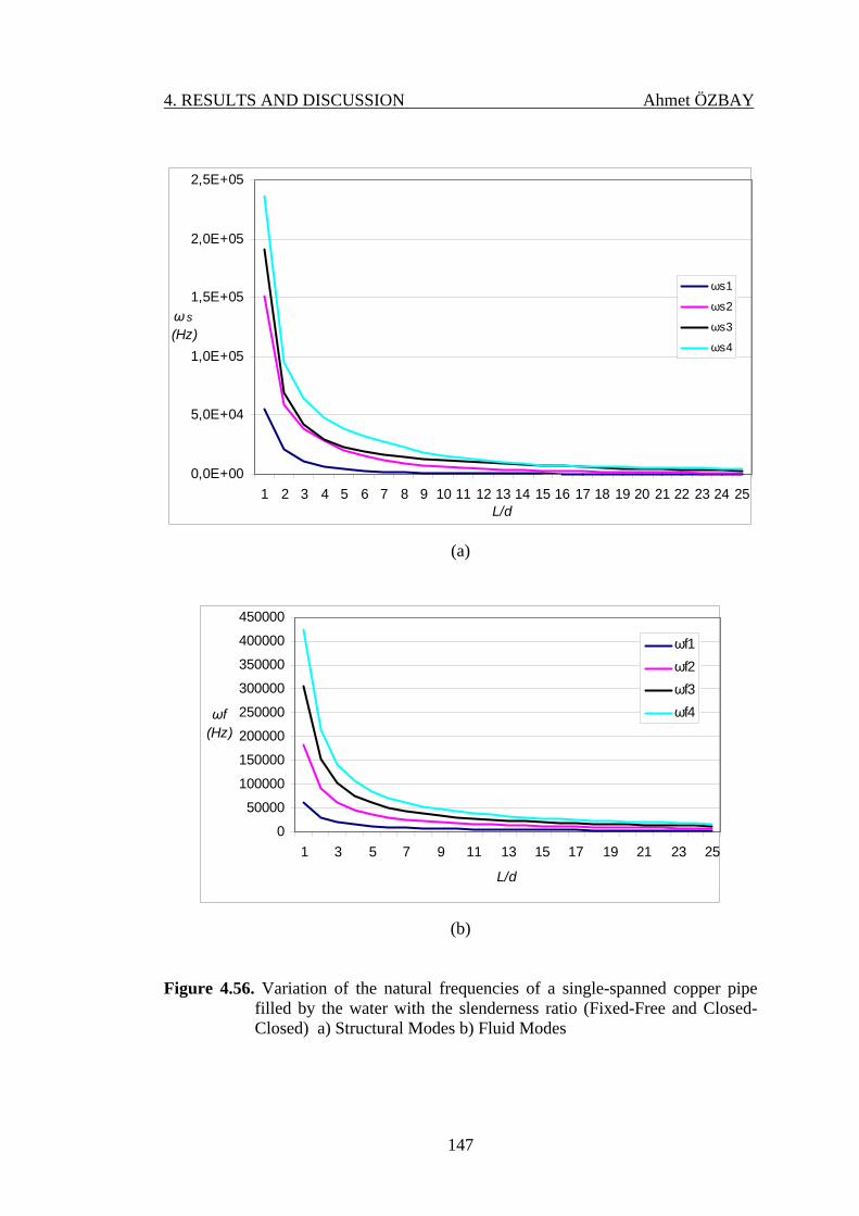
4. RESULTS AND DISCUSSION Ahmet ÖZBAY
147
0,0E+00
5,0E+04
1,0E+05
1,5E+05
2,0E+05
2,5E+05
1 2 3 4 5 6 7 8 9 10 11 12 13 14 15 16 17 18 19 20 21 22 23 24 25L/d
ω s(Hz)
ωs1
ωs2
ωs3
ωs4
(a)
0
50000
100000
150000
200000
250000
300000
350000
400000
450000
1 3 5 7 9 11 13 15 17 19 21 23 25
L/d
ωf (Hz)
ωf1ωf2ωf3ωf4
(b)
Figure 4.56. Variation of the natural frequencies of a single-spanned copper pipe filled by the water with the slenderness ratio (Fixed-Free and Closed-Closed) a) Structural Modes b) Fluid Modes

4. RESULTS AND DISCUSSION Ahmet ÖZBAY
148
4.6.2. Effect of the Bend-Angle on the Natural Frequencies
Here the bend angle between the axes of pipes is measured in counter-
clockwise direction as shown in Figure 4.57. Each section of pipe is assumed to be
equal (L1=L2=1m). The problem is studied for both fixed-fixed and fixed-free
structural boundary conditions. The pipe system is assumed to be made of either the
steel or the copper material. Only structured modes considered in this work
Figure 4.57. Bended Angle α
Variation of the natural frequencies in Hz of such pipe system with the bend
angle for different structural boundary conditions are demonstrated in Figures 4.58-
4.61. Some numerical results are tabulated in Tables 4.66-4.69.
α L1
L2
ITD
Highlight
ITD
Highlight
ITD
Highlight

4. RESULTS AND DISCUSSION Ahmet ÖZBAY
149
Table 4.66. Variation of the natural frequencies in Hz of steel pipe system with the bend angle (Fixed-Fixed)
Natural frequencies
Structural modes
Filled
by
)( °α 1ω 2ω 3ω 4ω
15 570 1.571 1.572 1.162 30 563 1.571 1.574 1.398 45 555 1.571 1.575 1.596 90 546 1.571 1.577 1.750 105 536 1.570 1.579 1.865 120 526 1.570 1.581 1.950 135 515 1.570 1.584 2.011 150 504 1.569 1.587 2.057 165 493 1.569 1.591 2.092
Air
175 482 1.568 1.595 2.119 15 473 965 1.304 1.305 30 467 1.163 1.303 1.306 45 461 1.327 1.303 1.307 90 453 1.456 1.303 1.308 105 445 1.551 1.303 1.310 120 436 1.621 1.303 1.312 135 427 1.672 1.302 1.315 150 418 1.709 1.302 1.317 165 409 1.738 1.302 1.321
Water
175 400 1.759 1.301 1.324

4. RESULTS AND DISCUSSION Ahmet ÖZBAY
150
Table 4.67. Variation of the natural frequencies in Hz of copper pipe system with the bend angle (Fixed-Fixed)
Natural frequencies
Structural modes
Filled
by
)( °α 1ω 2ω 3ω 4ω
15 178 566 498 499 30 176 628 498 499 45 174 661 498 500 90 171 680 498 500 105 167 691 498 501 120 164 698 498 502 135 160 703 498 503 150 157 706 498 504 165 153 709 498 505
Air
175 150 711 498 506 15 135 429 377 377 30 133 476 377 378 45 131 500 377 378 90 129 514 377 378 105 127 523 377 379 120 124 528 377 379 135 121 532 377 380 150 119 534 377 381 165 116 536 377 382
Water
175 113 538 377 383

4. RESULTS AND DISCUSSION Ahmet ÖZBAY
151
Table 4.68. Variation of the natural frequencies in Hz of steel pipe system with the bend angle (Fixed-Free)
Natural frequencies
Structural modes
Filled
by
)( °α 1ω 2ω 3ω 4ω
15 92 93 549 554 30 93 93 533 541 45 93 94 514 526 90 94 95 494 509 105 95 96 475 491 120 96 97 455 473 135 97 99 436 456 150 98 100 418 438 165 99 102 402 422
Air
175 101 104 386 406 15 77 77 455 464 30 77 78 442 457 45 77 78 427 448 90 78 79 411 437 105 79 81 395 425 120 79 82 378 413 135 80 83 363 400 150 81 85 348 387 165 82 87 334 375
Water
175 84 89 321 362

4. RESULTS AND DISCUSSION Ahmet ÖZBAY
152
Table 4.69. Variation of the natural frequencies in Hz of copper pipe system with the bend angle (Fixed-Free)
Natural frequencies
Structural modes
Filled
by
)( °α 1ω 2ω 3ω 4ω
15 29 29 171 173 30 29 29 166 169 45 29 29 160 165 90 29 29 154 159 105 29 30 148 154 120 30 30 141 148 135 30 31 135 143 150 30 31 130 137 165 31 32 124 132
Air
175 31 32 120 127 15 22 22 130 133 30 22 22 126 131 45 22 22 121 129 90 22 23 117 126 105 22 23 112 123 120 22 23 107 120 135 23 24 102 117 150 23 24 98 114 165 23 25 94 110
Water
175 24 26 90 107

4. RESULTS AND DISCUSSION Ahmet ÖZBAY
153
0,E+00
5,E+02
1,E+03
2,E+03
2,E+03
3,E+03
5 15 25 35 45 55 65 75 85 95 105
115
125
135
145
155
165
175
Bend Angle (α)
ω s(Hz)
ωs1
ωs2
ωs3
ωs4
a) Filled by the Air
0,E+00
2,E+02
4,E+02
6,E+02
8,E+02
1,E+03
1,E+03
1,E+03
2,E+03
2,E+03
2,E+03
5 15 25 35 45 55 65 75 85 95 105
115
125
135
145
155
165
175
Bend Angle (α)
ωs ωs1
ωs2
ωs3
ωs4
b) Filled by the Water
Figure 4.58. Variation of the natural frequencies (Hz) in structural modes of steel
pipe system with the bend angle (Fixed-Fixed)

4. RESULTS AND DISCUSSION Ahmet ÖZBAY
154
0,E+00
1,E+02
2,E+02
3,E+02
4,E+02
5,E+02
6,E+02
5 15 25 35 45 55 65 75 85 95 105
115
125
135
145
155
165
175
Bend Angle(α)
ωs (Hz)
ωs1ωs2ωs3ωs4
a) Filled by the Air
0
50
100
150
200
250
300
350
400
450
500
5 15 25 35 45 55 65 75 85 95 105
115
125
135
145
155
165
175
Bend Angle (α)
ω s(Hz)
ωs1ωs2ωs3ωs4
b) Filled by the Water
Figure 4.59. Variation of the natural frequencies (Hz) in structural modes of steel
pipe system with the bend angle (Fixed-Free)

4. RESULTS AND DISCUSSION Ahmet ÖZBAY
155
0
100
200
300
400
500
600
700
800
0 10 20 30 40 50 60 70 80 90 100
110
120
130
140
150
160
170
180
Bend Angle (α)
ω s(Hz) ωs1
ωs2ωs3ωs4
a) Filled by the Air
0
100
200
300
400
500
600
5 15 25 35 45 55 65 75 85 95 105
115
125
135
145
155
165
175
Bend Angle (α)
ωs (Hz) ωs1
ωs2
ωs3
ωs4
b) Filled by the Water
. Figure 4.60. Variation of the natural frequencies (Hz) in structural modes of copper
pipe system with the bend angle (Fixed-Fixed)
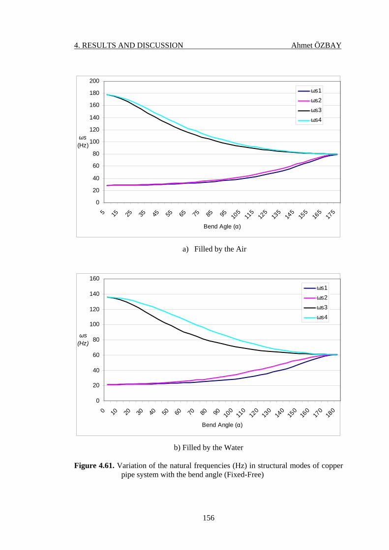
4. RESULTS AND DISCUSSION Ahmet ÖZBAY
156
0
20
40
60
80
100
120
140
160
180
200
5 15 25 35 45 55 65 75 85 95 105
115
125
135
145
155
165
175
Bend Agle (α)
ωs(Hz)
ωs1ωs2ωs3ωs4
a) Filled by the Air
0
20
40
60
80
100
120
140
160
0 10 20 30 40 50 60 70 80 90 100
110
120
130
140
150
160
170
180
Bend Angle (α)
ωs(Hz)
ωs1ωs2ωs3ωs4
b) Filled by the Water
Figure 4.61. Variation of the natural frequencies (Hz) in structural modes of copper
pipe system with the bend angle (Fixed-Free)

5. CONCLUSION Ahmet ÖZBAY
157
5. CONCLUSION
As is well known liquid-filled piping systems are very important for
many industrial applications. They are used for conveying gases and fluids over a
wide range of temperatures and pressures.
In this study, the free un-damped vibrational behavior of air/water-filled
piping systems is first studied with the help of the transfer matrix method (TMM).
The transfer matrix method provides a quick and efficient analysis of such systems.
The existence of bends, springs, orifices, valves, accumulators, pumps, and such
control instrumentations may be modeled easily in the transfer matrix method
without increasing the dimensions of the system matrices.
The closed-form governing equations available in the literature, which
consider the axial, transverse and torsional vibration of such piping systems, are
completely used in this work.
The fluid is assumed to be one-dimensional (the radial component of the fluid
velocity is zero and the flow is developed in only the axial direction), linear, and
homogeneous, with isotropic flow and uniform pressure and fluid velocity over the
cross-section. The fluid density is taken as constant (the convective terms are ignored
by assuming low Mach numbers, where the fluid wave speed is much greater than
the fluid velocity). The fluid friction term is neglected.
The pipe wall is assumed to be linearly elastic, isotropic, prismatic, circular
and thin-walled.
In the case studies considered in this thesis five different configurations of
piping systems made of either one inch-nominal diameter copper or two inch-
nominal diameter steel such as
• Single-spanned
• L-bended
• Z-bended
• U-bended
• 3-D bended
ITD
Highlight
ITD
Highlight

5. CONCLUSION Ahmet ÖZBAY
158
are studied with two main structural boundary conditions namely fixed-fixed and
fixed-free. Intermediate rigid support is also studied in this work. Fluid boundary
conditions are assumed to be closed at both ends. As a light fluid both the air and the
water are considered.
The theoretical frequencies based on the transfer matrix method are supported
by some experiments performed in this study.
The effect of the elastic foundation on the natural frequencies is also
investigated.
A parametric study is, finally, carried out to understand correctly the
vibrational behavior of such piping systems. Variation of the natural frequencies of
the pipe system with the slenderness ratio and the bend angle are illustrated by
graphs.
The results obtained in this work are verified by both finite element solution
using ANSYS and some results available in the literature. A very good harmony is
observed among the literature, experimental and theoretical results.

159
REFERENCES
AKDOĞAN, İ., 1992, Dynamic Analysis Of Piping Systems Using Transfer Matrix
Method, MSc. Thesis, METU.
ALLISON, A. E., 1998, Analytical Investigation of a Semi-Empirical Flow Induced
Vibration Model, PhD Thesis, The University of Western Ontario.
AUXWORTHY, D. H., 1998, Water Distribution Network Modeling From
Waterhammer, PhD Thesis, University of Toronto.
BAASIRI, M. S., 1981, A Quantitative Study of Free Air Release During Transient
Flow, PhD Thesis, Utah State University.
BRENNEN C. E., and ACOSTA, A. J., 1976, The Dynamic Transfer Function for a
Cavitating Inducer, journal of Fluids Engineering, Vol. 98,182, pp. 182-191.
BRENNEN C. E., ACOSTA, A. J. and GAUGHEY, T. K., 1986, Impeller Fluid
Forces, Nasa Conference Publication, 2436, Vol. 1, pp. 270-295.
BUDNY, D. D., 1988, Influence of Structural Damping on The Internal Fluid
Pressure During a Fluid Transient Pipe Flow, PhD Thesis, Michigan State
University.
COLLINA, A., ZANABONI, P., and BELLOLI, M., 2005, On the Optimization of
Support Positioning and Stiffness for Piping Systems on Power Plants, 18th
International Conference on Structural Mechanics in Reactor Technology,
ÇINAR, A., 1998, Boru Hatlarının Dinamiği ve Sönüm Modelleri, PhD Thesis, İTÜ.
DOLASA, A. R., 1998, Computer-Aided Design Software for the Undamped Two-
Dimensional Static and Dynamic Analysis of Beams and Rotors, MSc.
Thesis, Virginia Polytechnic Institute.
DURRANI, J. N., 2001, Dynamics Of Pipelines With A Finite Element Method,
MSc. Thesis, University of Calgary.
EVANS, R. P., 2004, Mass Flow Measurement Trough Flow-Induced Pipe
Vibration, PhD Thesis, Idaho State University.
GIDI, A., 1999, Two- Phase Flow-Induced Vibrations in a Heated Tube Bundle, PhD
Thesis, McMaster University.
ITD
Highlight
ITD
Highlight

160
HAKTANIR, V., 1990, Silindirik Helisel Çubukların Statik, Dinamik ve Burkulma
Davranışlarının Taşıma ve Rijitlik Matrisleri Metodu ile İncelenmesi”, PhD
Thesis, Ç.Ü.
HORNER, G. C., 1975, The Riccatti Transfer Matrix Method, PhD Thesis, The
Virginia University.
KARTHA, S. C., 2000, Active, Passive and Active Passive Control Techniques for
Reduction of Vibrational Power Flow in Fluid Filled Pipes, MSc. Thesis,
Virginia Polytechnic Institute.
KOO, G. H., and PARK, Y. S., 1998, Vibration Reduction By Using Periodic
Supports in a Piping System, Journal of Sound and Vibration, Vol. 210,
pp.53-68.
LESMEZ, M., W., 1989, Modal Analysis Of Vibrations In Liquid –Filled Piping
Systems, PhD Thesis, Michigan State University.
LI, M., 1997, An Experimental And Theoretical Study Of Fluidelastic Instability in
Cross Flow Multi-Span Heat Exchanger Tube Arrays, PhD Thesis, McMaster
University.
LIEW, A., FENG, N. S., and HAHN, E. J., 2004, On Using the Transfer Matrix
Formulation For Transient Analysis of Nonlinear Rotor Bearing Systems,
International Journal of Rotating Machinery, Vol. 10, pp. 425-431.
NIEVES, V. R., 2004, Static and Dynamic Analysis of a Piping System, MSc.
Thesis, University of Puerto Rico.
OTWELL, R. S., 1984, Efect Of Elbow Restraint on Pressure Transients, PhD
Thesis, Michigan State University.
PESTEL, E. C., and LECKIE, F. A., 1963, Matrix Methods in Elostomechanics,
McGraw-Hill, New York.
RUNGTA, R., 1998, Separation Criteria of Fluid Piping Systems Using a Lumped-
Parameter Method, MSc. Thesis, The University of Western Ontario.
SERVAITES, J. C., 1996, Computer Aided Analyses of Smoke Stack Designs, MSc.
Thesis, Virginia Polytechnic Institute.
ITD
Highlight
ITD
Highlight
ITD
Highlight
ITD
Highlight

161
TENG-YANG, R., 1998, Measurement of Flow Induced Vibration And Flow
velocities in a Scaled Model of The Flixborough “Dog-Leg” Pipe, MSc.
Thesis, The University of New Brunswick.
YU, J. F., 2001, Vibration And Sensitivity Analysis of Structures With Optimal
Design Using Transfer Dynamic Stiffness Matrix, PhD Thesis, The
University of Texas Arlington.
YAKUT, K., 1996, Dirsek ve Vanalı Boru Hatlarında Akış Kaynaklı Titreşimlerin
Spektral ve Gürültü Analizi, PhD Thesis, E.Ü.
ZHANG, Q., 2001, Lateral Vibration of Non-Rotating Drill Pipe Conveying Fluid in
Vertical Holes, PhD Thesis, The University of Tulsa.
ITD
Highlight

162
CURRICILUM VITAE
Ahmet ÖZBAY was born in Adana, 1976. After graduating from high school
in 1994, he enrolled in the University of Çukurova, Adana, where he received a
Bachelors of Science degree in Mechanical Engineering in 2000. In Fall of 2000 he
enrolled the University of Çukurova, Adana, where he completed his Masters of
Science degree in September, 2002. While obtaining this degree he was employed as
research assistant in the same department. He started his Doctor of Philosophy
education in the same institute in 2002. He has been working as a maintenance
engineer in soda ash plant, Mersin Soda Sanayii since 2005.

163
APPENDIX
A.1. ANSYS Source Codes for Fixed-Fixed Single Span Copper Pipe with Air. Source: /PREP7 ET,1,16 R,1,0.028,0.001,,,,1.2 MP,EX,1,97e9 MP,NUXY,1,0.35 MP,DENS,1,8350 N,1,0,0,0 N,11,0,0,2 FILL,1,11 E,1,2 EGEN,10,1,1,1,1 D,1,ALL D,11,ALL Results: ***** INDEX OF DATA SETS ON RESULTS FILE ***** SET TIME/FREQ LOAD STEP SUBSTEP CUMULATIVE 1 29.004 1 1 1 2 80.972 1 2 2 3 188.71 1 3 3
ITD
Highlight
ITD
Highlight
ITD
Highlight
ITD
Highlight
ITD
Highlight
ITD
Highlight
ITD
Highlight
ITD
Highlight

164
A.2. ANSYS Source Codes for L Bended Fixed-Fixed Steel Pipe with Water Source: /PREP7 ET,1,16 R,1,0.0635,0.0036,,,,997 MP,EX,1,157e9 MP,NUXY,1,0.28 MP,DENS,1,7600 N,1,0,0,0 N,11,0,0,2.4 FILL,1,11 N,21,2.4,0,2.4 FILL,11,21 E,1,2 EGEN,20,1,1,1,1 D,1,ALL D,21,ALL
Results:
SET TIME/FREQ LOAD STEP SUBSTEP CUMULATIVE 1 8.5859 1 1 1 2 32.124 1 2 2 3 33.675 1 3 3 4 46.451 1 4 4 5 48.734 1 5 5 6 104.78 1 6 6


![Free Vibration and Material Mechanical Properties ... · Free Vibration and Material Mechanical Properties ... The .iges file is imported in Ansys 14.5[1] ... the structure optimization](https://static.fdocuments.in/doc/165x107/5aed459f7f8b9a90318f6ed7/free-vibration-and-material-mechanical-properties-vibration-and-material-mechanical.jpg)