Three Dimensional Strain Field Morphing

Han-Bing YanTsinghua University

Beijing, Chinayanhb02@mails.tsinghua.edu.cn

Shi-Min Hu∗

Tsinghua UniversityBeijing, China

shimin@tsinghua.edu.cn

Ralph R. MartinCardiff University

Cardiff, UKralph@cs.cf.ac.uk

Abstract

In this paper, we present a new technique for 3D shapemorphing using strain fields. Strain is an important geomet-ric quantity used in mechanics to describe the deformationextent of objects. We use it to analyze and control deforma-tion in morphing. Using the position vector field, the strainfield between source and target shapes can be obtain. Thisstrain field is then interpolated between zero and its finalvalue to give the position field for intermediate shapes. Thismethod ensures that the 3D morphing process is smooth andno shape jittering or wobbling happens, and that locally,volumes suffer minimal distortion. We also show how tomodify the method so that changes of shape (in particular,lengths) vary linearly with time.

1 Introduction

Morphing, or metamorphosis, aims to generate a smoothshape sequence which transforms a source shape into a tar-get shape. This technique has become increasingly impor-tant in computer graphics for animation and entertainment,and is commonly employed by the special effects industry.Many morphing techniques have been developed for the 2Dcase [1]. With the introduction of 3D games and cartoons,3D morphing has gained in importance.

Methods for 3D morphing typically take one of two ap-proaches. The first blends volumes in which the initial andfinal shapes are embedded [2, 3, 4]. The other is based onmeshes, either 3D surface meshes or solid meshes. Thefirst approach has the advantage of being able to deal ob-jects with different topologies. However, in most cases, themesh method exhibits better results—often, shape bound-aries produced by the volume based method are not smoothenough. The method in this paper is based on meshes, andso henceforth we mainly consider mesh methods.

Usually, mesh morphing techniques involve two steps.The first is to find a mapping between the source and tar-get objects, which requires that both should be meshed in

an equivalent way—they should be meshedisomorphicallywith consistentmeshes. Having done this, the second stepis to choose a suitable path for each pair of correspondingpoints. Intermediate shapes have a mesh which is again iso-morphic to the initial and final meshes, with vertex locationsinterpolated for each particular time on the path.

Often, the source and target objects are already meshed,but not in a consistent way, so the first step involves takingthese meshes, and constructing a new mesh for both sourceand target which are consistent. Kent [5] introduced a topo-logical merging method to do this for star shaped objects,and other objects that can easily be projected onto a sphere,by merging the meshes in the spherical domain. Lazarus etal. [6] extended this idea to more general shapes. Alexa [7]proposed a method which uses spherical parameterizationto map source and target objects (of genus zero) onto asphere, then warps the spherical meshes to align features,and finally merges the two spherical meshes to give a con-sistent mesh.

Much work [8, 9, 10, 11, 12] is based on dissecting thesource and target shape into serveral pieces, and makinglocal parameterization on each piece, then using merging orremeshing methods to create a consistent mesh. Praun [13]gives a tracing method which can dissect the source andtarget shape automatically.

Both [7] and [11] present fast merging methods whichhave complexityO(n + k), wheren is the number of ver-tices andk is the number of interpolated points.

Lee [14] and Michikawa [15] proposed the use of mul-tiresolution methods to create consistent meshes.

All of these papers focus on the problem of creating con-sistent meshes, and most of them use simple linear interpo-lation methods for constructing corresponding point paths.For objects with similar shapes, linear interpolation to givepaths of points in the mesh is good enough for visual ef-fects. But for objects undergoing large deformation, espe-cially if bending occurs, linear interpolation always leadsto shrinkage of intermediate shapes, which is visually un-acceptable. In [16], instead of using other linear interpo-lation, Floater and Gotsman introduced barycentric coordi-

nate interpolation to find suitable paths. Blanding [17] et al.represent the interors of 3D shapes using compatible skele-tons and apply blending to the parametric description of theskeletons. Alexa [18] presented the use of interpolation ofLaplacian coordinates for the morphing path and discussedhow to control morphing locally. Hu [19] et al. presented amethod which minimizes deformation energy. This methodis novel in that it does not use interpolation, but a globaloptimization method.

A more effective method for coping with source andtarget shapes with large differences is presented in [20].This method first converts each surface polygon mesh intoa tetrahedral mesh. To perform morphing, it then finds atransformation which is locally as similar as possible to theoptimal transformation between each pair of correspondingtetrahedra. Optimization is used to minimize the differencebetween the desired transformation, and the actual transfor-mation which is applied, taking into account the connectiv-ity constraints on adjacent tetrahedra.

An alternative approach is proposed in [21, 22]. In thesemethods, consistent meshes are not required. They dynami-cally and adaptively change the connectivity of intermediatemeshes, and gradually transform the connectivity from thatof the source model into that of the target. It would seemdifficult for this method to get good results for shapes thatdiffer greatly.

For further discussion of previous work, the reader is re-ferred to the two excellent 3D morphing surveys by Lazarusand Alexa [23, 24].

The purpose of morphing is to create a smooth deforma-tion process. The path of each point in linear interpolationis also smooth, so why is its result not visually acceptable inmany cases? The reason is that it causes shapes to shrink inintermediate frames. Thus, a smooth deformation requiresnot only that each point path should be smooth, but alsothat shape should change in a monotonic manner. The mainproblem with previous 3D morphing methods is that theyhave not used an effective way to analyze object deforma-tion in detail.

In this paper, we propose a new morphing method for 3Dobjects, which is an extension of the 2D morphing methodof [25]. We give an approach which ensures that the de-formation process is uniform, and that squeezing or shrink-ing phenomena will not happen. Furthermore, we give ananalytical method to analyze and quantify the deformationextent of each intermediate shape.

2. Strain Fields

Our aim is to make shape deformation in the 3D mor-phing process natural and visually appealing. We want thedeformation in the morphing process to be uniform. Butwhat is deformation? In fact, local deformation at a point

is not equal to the displacement of this point. Points in anobject can have very small deformation though they havemoved a long distance, or conversely, they can have largedeformation but small displacement. In fact deformationconcerns how much a point is displacedrelative to neigh-boring points. Thus, deformation is an infinitesimal quan-tity. To analyze deformation, we need to use a tool frommechanics,strain. We start by giving definitions of the po-sition field and the strain field.

The positions of all points in a shape compose a field,which we call itsposition field. In 3D space, the positionfield has three components:[x, y, z]. When a shape movesor deforms, each point on the shape ends up in a new place[x′, y′, z′].

Using ideas from mechanics, the difference between asource shape and a target, or any intermediate shape, canbe decomposed into two parts: arigid body motion, and adeformation. The rigid body motion can be further decom-posed into a translation and rotation. In 3D, there are sixdegrees of freedom for rigid body motion, three for trans-lation and three for rotation. The deformation is separatelycaptured by astrain field, and is independent of rigid bodymotion. If only rigid body motion happens, without de-formation, although each point has displacement, the strainfield is zero.

Since for morphing we wish to handle large deforma-tions, in this paper we use large deformation formulae in-stead of the small deformation formulae most often used inmechanical engineering. In 3D, the strain field is a second-order tensor field, which has 6 independent components forhomogeneous materials:εx ,εy, εz are tension components,andγyz, γzx, γxy are shear components. In detail,εx ,εy,εz give the local infinitesimal scaling along each coordi-nate direction. They are positive in tension and negativein compression.γxy represents the relative change in anglebetween lines initially in thex andy directions at a givenpoint, and similarly forγyz andγzx. The relationship be-tween the strain field and the position field in 3D is givenby:

εx

εy

εz

γyz

γzx

γxy

=

12

[(∂x

′

∂x )2 + (∂y′

∂x )2 + (∂z′

∂x )2 − 1]

12

[(∂x

′

∂y )2 + (∂y′

∂y )2 + (∂z′

∂y )2 − 1]

12

[(∂x

′

∂z )2 + (∂y′

∂z )2 + (∂z′

∂z )2 − 1]

∂x′

∂y∂x′

∂z + ∂y′

∂y∂y′

∂z + ∂z′

∂y∂z′

∂z

∂x′

∂z∂x′

∂x + ∂y′

∂z∂y′

∂x + ∂z′

∂z∂z′

∂x∂x′

∂x∂x′

∂y + ∂y′

∂x∂y′

∂y + ∂z′

∂x∂z′

∂y

(1)

wherex, y andz are the position field components beforedeformation, andx′, y′ andz′ are components of the po-sition field after deformation. Thedisplacement fieldhascomponentsu, v,w, and is related to the position field byx′ = x + u, y′ = y + v, z′ = z + w.

2

Figure 1. Linear Interpolation

Figure 2. Strain Field Interpolation

In the following, the strain field is represented in vectorform, and we writeε for [εx, εy, εz, γyz, γzx, γxy]T . Weassume the shape varies from source to target over the timeinterval(0, 1) and we use a superscript to denote time. Forexample,ε1 means the strain field of the target shape, andεt means the strain field at timet.

Figures 1 and 2 are two results produced by linear inter-polation and strain field interpolation respectively. It is clearthat the result of strain field interpolation is more natural.The result in Figure 1 is poor because wobbling happens,and the elephant’s nose shrinks before extending again.

We now analyze strain change during these two morph-ing processes. In Figure 3 the strain curves for linear in-terpolation, and strain field interpolation, are ploted, for atetrahedron at the tip of the elephant’s trunk. Each figureshows six curves for the different components of strain. Forlinear interpolation, the curves forεz, γyz andγzx almostoverlap; In strain field interpolation,εy, εz, γyz andγzx arenearly identical. Note that in the case of linear interpola-tion, the curves ofεx andεy dip greatly during the morph-ing. This means that the tetrahedron is highly compressed atintermediate times. Finally, it is in tension and bigger. Thisanalysis is in agreement with the observed shape change inFigure 1. The analysis shows that using strain field inter-polation gives monotonic changes in strain, so the shape inFigure 2 changes in a monotonic way.

This example show that strain is an effective way to ana-lyze shape deformation.

Figure 3. Strain-Time Curve

3. Strain Field Morphing

3.1 Creating Consistent Tetrahedral Meshes

As noted in Section 1, there are two kinds of mesh usedin 3D morphing, surface (polygon) meshes [10, 14] andsolid (polyhedral) meshes [20]. Surface meshes have fewerelements and methods based on them take less computa-tional time. Solid meshes fill the interior of the shape in-stead of only its boundaries, and have the advantage thatmethods based on them find it easier to avoid volumeshrinkage, and generally result in less distortion. Here, toapply the concepts of strain, we use a solid tetrahedral meshto represent shape. Thus first, we need to create consistenttetrahedral meshes. For arbitrary shapes, we may need tocut complex shape into several genus-zero parts, and createconsistent meshes for each part.

Much work has been done on the creation of consistentmeshes in 3D [7, 13, 11], but most of it has only consid-ered surface meshes. However, Alexa et al. [20] give amethod for creating consistent tetrahedral meshes from sur-face meshes. We use this idea to create such meshes for

3

shapes of genus-zero. Assuming we are given source andtarget objects represented as surface meshes, first, we con-vert each surface mesh to a solid tetrahedron mesh, usingGeopack or some other commercial finite element softwarepackage. Then each genus-zero surface is parameterizedon a sphere in such a way that features are aligned as themethod in [7]. These features are the ones chosen by theuser to be in correspondence in the source and target shapes.Next, inner points of each tetrahedral mesh are mapped intothe sphere using barycentric coordinates, and the source andtarget mesh mapped into the sphere are merged togetherto create a consistent mesh. Finally, this mesh inside thesphere is mapped back to the original objects.

Unfortunately, we have found that, when using barycen-tric coordinates to map the inner points into the sphere, cer-tain tetrahedra have negative volume, i.e. flipped orienta-tions. The problem is that the barycentric coordinate param-eterization method which works well in 2D does not extendto 3D in the same way. We note that while this method isused in [20], its correctness is not proved. We use an inter-active method to adjust inner vertex positions to solve thisproblem. We also investigated using linear and nonlinearspring models to give a 3D parameterization. The linear ap-proach also suffers from the flip problem. The nonlinearapproach suffers from poorly conditioned equations, andagain it is not easy to get a satisfactory result. Clearly, suit-able parameterization methods for tetrahedral meshes stillneed further study.

3.2 Removing the Rigid Body Motion

Strain is independent of rigid body motion. The overallmetamorphosis comprises a deformation plus a rigid bodymotion, and we need to separate out the the latter so that wecan consider the strain by itself.

A rigid body has 6 degrees of freedom in 3D space.To factor out the rigid body motion, we select three cor-responding points on source and target shapes,A0, B0, C0,andA1, B1, C1, and then place the source and target shapesin a canonical position and orientation. The source shape ismoved untilA0 coincides with the origin, the translationvector necessary beingT 0. Then the source mesh is rotatedaround origin point untilB0 lies on thex axis. Let the rota-tion axis beR0, with angle isθ0

α. Finally, the source mesh isrotated around thex axis untilC0 is on thex−y plane withpositivey component; the angle of rotation isθ0

β . The tar-get shape treated similarly, with corresponding parametersT 1, R1, θ1

α andθ1β . Thex, y, z coordinates ofA, they, z

coordinates ofB, and thez coordinate ofC are then fixedduring the entire deformation process, and the rigid bodycomponent of metamorphosis is only added back as a fi-nal computation after the deformation has been determined(see Section 3.5). The points chosen to determine the rigid

body motion can be selected by the computer automatically,or interactively by the user.A0 andA1 should be selectednear the center of the source and target shapes, whileB0,B1, C0 andC1 should lie along the shape’s ‘natural’ axes.

3.3 Intermediate Strain Field Calculation

The strain field for shapes in between the source and tar-get shapes can be calculated using ideas from Eqn. 1. Weuse tetrahedral elements, as often used in thefinite elementmethod(FEM), to calculate the strain field. Because, unlikeengineering analysis, morphing does not require high preci-sion results, it is sufficient to use linear tetrahedral elementsrather than higher order elements. In FEM, each point in anelement can be expressed as a convex combination of thepositions of the element’s nodes:

x =l∑

k=1

Nkxk, y =l∑

k=1

Nkyk, z =l∑

k=1

Nkzk, (2)

whereNk is theshape functionof the element, andl is thenumber of vertices of the element. For linear tetrahedralelements,Nk are barycentric coordinates within the tetra-hedron. Substituting Eqn. 2 into Eqn. 1, we can convert thestrain field calculation into discrete form. Using nodes co-ordinates of source and target shapes in Eqn. 1 and Eqn. 2,the strain field relating source and target shapes can be cal-culated.

The simplest way to choose a strain field for intermediateshapes is to use linear interpolation:

εt = (1− t)ε1; (3)

note thatε0 is zero.Linear strain interpolation usually produces good mor-

phing results for most examples, but in some extreme cases,linear strain interpolation gives uneven rates of change ofshape over time, even though at each intermediate time theshape itself is good. In Section 3.6, we analyse this problemfurther, and provide an alternative method of interpolationfor such extreme cases.

3.4 From Strain Field to Position

We now have the strain field at any desired time. Thestrain field has six components, and the position field hasthree components. It can be seen that the six components instrain field are thus not independent, and they are connectedby a set of compatibility equations [26]. In general, thismeans that arbitrarily interpolated strain fields do not cor-respond to physically realisable position fields. Thus, weattempt to find a position field for the intermediate shapewhose strain field is as close as possible to the interpolated

4

strain field. We define an energy function in Eqn. 4 whichcomputes the norm of the difference between a given inter-polated strain field and the strain field generated by someposition field:

W =12

∫(ε′ − ε)T · (ε′ − ε)dΩ. (4)

Ω is taken over the whole source shape,ε is the interpolatedstrain field, andε′ is calculated from the position field us-ing Eqn 1. We try to find a position field which minimizesthis energy function to give the intermediate shape. Thisproblem can be solved by any multi-variable optimizationmethod, whose variables are coordinates of all nodes in theintermediate shape.

In practice, for efficiency, we convert this optimisationproblem into a set of non-linear equations by calculatingthe derivative of Eqn. 4. The approach follows closely thatfor the 2D case in [25], and here we only give the final resultin 3D. The non-linear equation system can be written as:

φ(V ) = 0 (5)

whereV is the coordinate vector of the intermediate shape.φ(V ) has the form

φ(V ) =m∑

i=1

∫(BT ε′ −BT ε)dΩi, (6)

wherem is the number of tetrahedra, andB is the strainmatrix. B can be written as

B = [B1xB1yB1zB2xB2yB2zB3xB3yB3zB4xB4yB4z],

whereBiu is defined as

Biu =

∂ut

∂x∂Ni

∂x∂ut

∂y∂Ni

∂y∂ut

∂z∂Ni

∂z∂ut

∂y∂Ni

∂z + ∂ut

∂z∂Ni

∂y∂ut

∂z∂Ni

∂x + ∂ut

∂x∂Ni

∂z∂ut

∂x∂Ni

∂y + ∂ut

∂y∂Ni

∂x

; (7)

Ni are the shape functions.This non-linear equation can be solved by Newton-

Raphson method. We generally wish to calculate the po-sition field for a series of intermeidate shapes. The coordi-nate vector for the source shape is used as the initial valuefor iterative calculation of the coordinate vector for the firstintermediate shape, and the calculation for each subsequentintermediate shape is initialized using the coordinate vectorof the previous intermediate shape. This method gives goodinitial values, and ensures convergence. Because we havegood initial values, our method is also fast. If the num-ber of intermediate shapes required is very small, Eqn. 5could also be solved by using a continuation method, but inpractice, simply adding more intermediate shapes is moreefficient.

3.5 Incorporating Rigid Body Motion

Deformations for intermediate shapes were determinedin the previous Section. Now, an appropriate rigid body mo-tion must also be incorporated to give the final intermediateshape in its correct position and orientation. We simply re-verse the process given in Section 3.2, adding in an linearlyinterpolated translation and roation. First we rotate the in-termediate shape at timet around thex axis by the angle:

θtβ = −[(1− t)θ0

β + tθ1β ]. (8)

Then we find the axis of rotation

Rt = (1− t)R0 + tR1 (9)

and rotate around this axis by the angle

θtα = −[(1− t)θ0

α + tθ1α]. (10)

Finally, the intermediate shape is translated by:

T t = −[(1− t)T 0 + tT 1] (11)

giving the desired result.

3.6 Modified Interpolation Method

Using linear interpolation of strain as described in Sec-tion 3.3 often produces good results. However, in a few ex-treme cases where the deformation is very large, althougheach intermediate shape has good shape, shape change mayoccur unevenly with respect to time. The reason of this phe-nomenon is that Eqn. 1 includes quadratic terms.

In fact, many morphing methods suffer from unevenchanges over time, but unlike other methods, in the caseof strain field morphing we can find a theoretically-basedmodification to the method to at least partially compensatefor this. The basis of this modification is to force the lengthsof edges parallel to the coordinate axes change linearly withtime, which also constrains the length change ratio in otherdirections. Appropriate background ideas from mechanicscan be found in [26, 27].

In essence, the strain field arises due to length changesin line segments. Consider an infinitesimal line segmentPQ in the source shape. Let the coordinates ofP be(ax, ay, az), or a for short. Let the coordinates ofQ be(ax + dax, ay + day, az + daz). Let the length ofPQ bedS0. The corresponding line segment in the target shape isP 1Q1, of lengthdS1. The relation betweendS0 anddS1

is:

(dS1)2 − (dS0)2 = 2da · E1 · da (12)

(dS0)2 = da · da (13)

5

Figure 4. Twisting a Rod

Figure 5. Helix

Figure 6. Animal Morphing

6

whereda is the vector(dax, day, daz), andE1 is the matrixform of the strain field tensor for the target mesh. A generalstrain field tensorE has the form:

E =

εx γxy γxz

γxy εy γyz

γxz γyz εz

. (14)

The length of segmentPQ at timet has a similar relation tothe length of in the source shape:

(dSt)2 − (dS0)2 = 2da · Et · da (15)

If we want the length ofPQ to change linearly with time,we should let:

dSt − dS0

dS1 − dS0= t (16)

Substituting Eqns. 12 and 15 into Eqn. 16, we obtain

(dS0)2 + 2daEtda = (17)[t√

(dS0)2 + 2daE1da + (1− t)dS0]2

For a line segment parallel to thex axis,da is:

da = [dax, 0, 0]. (18)

Substituting Eqn. 18 into Eqn. 18, and using Eqn. 13, wefind that:

εtx =

12

[[t√

1 + 2ε1x + (1− t)]2

− 1]

(19)

Similarly we may show that

εty =

12

[[t√

1 + 2ε1y + (1− t)]2

− 1]

(20)

εtz =

12

[[t√

1 + 2ε1z + (1− t)]2

− 1]

(21)

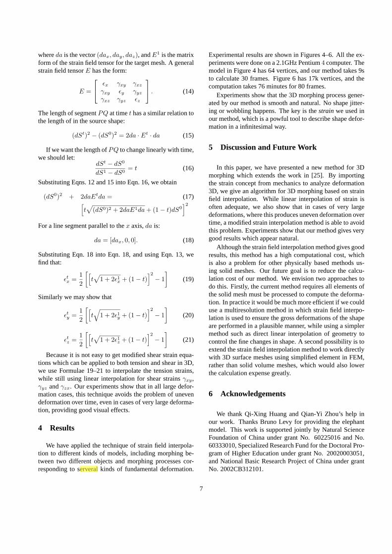
Because it is not easy to get modified shear strain equa-tions which can be applied to both tension and shear in 3D,we use Formulae 19–21 to interpolate the tension strains,while still using linear interpolation for shear strainsγxy,γyz andγzx. Our experiments show that in all large defor-mation cases, this technique avoids the problem of unevendeformation over time, even in cases of very large deforma-tion, providing good visual effects.

4 Results

We have applied the technique of strain field interpola-tion to different kinds of models, including morphing be-tween two different objects and morphing processes cor-responding to serveral kinds of fundamental deformation.

Experimental results are shown in Figures 4–6. All the ex-periments were done on a 2.1GHz Pentium4 computer. Themodel in Figure 4 has 64 vertices, and our method takes 9sto calculate 30 frames. Figure 6 has 17k vertices, and thecomputation takes 76 minutes for 80 frames.

Experiments show that the 3D morphing process gener-ated by our method is smooth and natural. No shape jitter-ing or wobbling happens. The key is thestrain we used inour method, which is a powful tool to describe shape defor-mation in a infinitesimal way.

5 Discussion and Future Work

In this paper, we have presented a new method for 3Dmorphing which extends the work in [25]. By importingthe strain concept from mechanics to analyze deformation3D, we give an algorithm for 3D morphing based on strainfield interpolation. While linear interpolation of strain isoften adequate, we also show that in cases of very largedeformations, where this produces uneven deformation overtime, a modified strain interpolation method is able to avoidthis problem. Experiments show that our method gives verygood results which appear natural.

Although the strain field interpolation method gives goodresults, this method has a high computational cost, whichis also a problem for other physically based methods us-ing solid meshes. Our future goal is to reduce the calcu-lation cost of our method. We envision two approaches todo this. Firstly, the current method requires all elements ofthe solid mesh must be processed to compute the deforma-tion. In practice it would be much more efficient if we coulduse a multiresolution method in which strain field interpo-lation is used to ensure the gross deformations of the shapeare performed in a plausible manner, while using a simplermethod such as direct linear interpolation of geometry tocontrol the fine changes in shape. A second possibility is toextend the strain field interpolation method to work directlywith 3D surface meshes using simplified element in FEM,rather than solid volume meshes, which would also lowerthe calculation expense greatly.

6 Acknowledgements

We thank Qi-Xing Huang and Qian-Yi Zhou’s help inour work. Thanks Bruno Levy for providing the elephantmodel. This work is supported jointly by Natural ScienceFoundation of China under grant No. 60225016 and No.60333010, Specialized Research Fund for the Doctoral Pro-gram of Higher Education under grant No. 20020003051,and National Basic Research Project of China under grantNo. 2002CB312101.

7

References

[1] Wolberg G (1998) Image Morphing: a survey. The VisualComputer 14(12):360-372

[2] Cohen-Or D, Levin D, Solomovoci A (1998)Three dimen-sional distance field metamorphosis. ACM Trans Graph17:116-141

[3] Lerios A, Garfinkle CD, Levoy M (1995) Featurebasedvolume metamorphosis. Comput Graph (SIGGRAPH’ 95)29:449-464

[4] X. Fang, H. Bao, P. A. Heng, T. T. Wong and Q. Peng (2001)Continuous field based free-form surface modeling and mor-phing. Computer and Graphics 25(2):235-243

[5] Kent JR, Carlson WE, Parent RE (1992) Shape transforma-tion for polyhedral objects. Comput Graph (SIGGRAPH’92) 26:47-54

[6] Lazarus F, Verroust A (1997) Metamorphosis of cylinder-like objects. Int J Visualization Comput Anim 8:131-146

[7] M. Alexa (2000) Merging polyhedral shapes with scatteredfeatures. The Visual Computer, 16(1):26-37

[8] H. Bao and Q. Peng (1998) interactive 3d morphing. Com-puter Graphics Forum, 17(3):23-30

[9] A. Gregory, A. State, M. Lin, D. Manocha, and M. Liv-ingston (1998) Feature-based surface decomposition for cor-respondence. Computer Animation 98, Philadelphia, Penn-sylvania, USA

[10] T. Kanai, H. Suzuki, F Kimura(1998)Three-dimensional ge-ometric metamorphosis based on harmonic maps.The VisualComputer,14:166-176

[11] TY Lee, PH Huang(2003)Fast and Intuitive Metamorpho-sis of 3D Polyhedral Models Using SMCC Mesh Merg-ing Scheme, IEEE Trans. Visualizaton Comput Graphics,9(1):85-98

[12] JB Yu, JH Chuang(2003)Consistent Mesh Parameterizationsand Its Application in Mesh Morphing ,Computer GraphicsWorkshop 2003

[13] E. Praun, W. Sweldens, and P. Schroder(2001)Consistentmesh parameterizations. Proceedings of SIGGRAPH 2001,179-184

[14] A. Lee, D. Dobkin, W. Sweldens, and P. Schroder(1999)Multiresolution mesh morphing. Proceedings of SIG-GRAPH 1999, 343-350

[15] T. Michikawa, T. Kanai, M. Fujita, and H. Chiyokura(2001)Multiresolution interpolation meshes. In 9th Pacific Confer-ence on Computer Graphics and Applications, 60-69

[16] M. S. Floater and C. Gotsman(1999) How to morph tilingsinjectively. Journal of Computational and Applied Mathe-matics, 101:117C129,

[17] Turkiyyah, Storti, and Ganter(2000) Skeletonbased three-dimensional geometric morphing. CGTA: ComputationalGeometry: Theory and Applications, 15, 2000,

[18] M. Alexa (2001) MLocal control for mesh morphing. Pro-ceedings of the International Conference on Shape Model-ing and Applications, 209-215

[19] SM Hu, CF Li and H Zhang(2004) Actual Morphing: Aphysical-based Approach for Blending, ACM Symposiumon Solid Modeling and Application 2004

[20] M. Alexa, D. Cohen-Or, and D. Levin(2000)As-rigidas-possible shape interpolation, Proceedings of SIGGRAPH2000, 157-164

[21] CH Lin and TY Lee(2004)Metamorphosis of 3D Polyhe-dral Models Using Progressive Connectivity Transforma-tions, IEEE Trans. Visualizaton Comput Graphics, 10(6):1-1

[22] TY Lee, CC Huang(2005)Dynamic and Adaptive Morph-ing of Three-Dimensional Mesh Using Control Maps, IEICETrans. Inf. and Syst, 88(3):646-651

[23] F. Lazarus and A. Verroust(1998) Three-Dimensional Meta-morphosis: A Survey, The Visual Computer, 14:373-389

[24] M. Alexa (2001) Recent Advances in Mesh Morphing. Com-puter Graphics Forum

[25] HB Yan, SM Hu and Ralph Martin(2004)Morphing Basedon Strain Field Interpolation, Int J Visualization ComputAnim 15:443-452

[26] Flugge, Wilhelm(1972) Tensor analysis and continuum me-chanics, Springer-Verlag,c1972

[27] O.C.Zienkiewicz(2000)The finite element method.McGraw-Hill 2000

8