THREE-DIMENSIONAL RECONSTRUCTION OF THE VIRTUAL PLANT ...

THREE-DIMENSIONAL RECONSTRUCTION OF THE VIRTUAL PLANT BRANCHING

STRUCTURE BASED ON TERRESTRIAL LIDAR TECHNOLOGIES AND L-SYSTEM

Yinxi Gong1,2, Yanqin Yang1,2, Xiaofen Yang1,2

1. National Administration of Surveying, Mapping and Geoinformation engineering research center of Geographic National

Conditions Monitoring, Xian 710000, China; 2.The First Institute of Photogrammetry and Remote Sensing, Xian 710000, China;

KEY WORDS: Terrestrial LiDAR, L-system, Branching structure, Point cloud data, Topology structure

ABSTRACT:

For the purpose of extracting productions of some specific branching plants effectively and realizing its 3D reconstruction,

Terrestrial LiDAR data was used as extraction source of production, and a 3D reconstruction method based on Terrestrial LiDAR

technologies combined with the L-system was proposed in this article. The topology structure of the plant architectures was extracted

using the point cloud data of the target plant with space level segmentation mechanism. Subsequently, L-system productions were

obtained and the structural parameters and production rules of branches, which fit the given plant, was generated. A three-

dimensional simulation model of target plant was established combined with computer visualization algorithm finally. The results

suggest that the method can effectively extract a given branching plant topology and describes its production, realizing the extraction

of topology structure by the computer algorithm for given branching plant and also simplifying the extraction of branching plant

productions which would be complex and time-consuming by L-system. It improves the degree of automation in the L-system

extraction of productions of specific branching plants, providing a new way for the extraction of branching plant production rules.

1. INTRODUCTION

As the structure of branching plants closely related to the

process of their growth and development, accurately and

quickly simulating three-dimensional (3D) structure of the

branching plants can effectively and precisely show the process

of plant growth and development, and reflect the growth law. In

recent years, as the increasing cross fusion of life science and

information science, it is possible to digitize the structures and

functions of plants and thus achieve a precise description, visual

expression, development evaluation, quantitative calculation,

simulation and prediction of the plant morphology. And it has

become an important and developing direction of the

contemporary agricultural science and forestry production

(Prusinkiewicz, 2004). Virtual plant has been taken as a useful

tool to understand complex relationship among plant gene

function, plant growth, plant physiology and plant form.

A series of Worldwide research has been conducted on the

structure model of virtual plants, and significant results have

been achieved (Zhao, De Reffye, Xiong Hu, Zhan, 2001).

Primarily, they are the Lindenmayer system (L-system) put

forward by American biologist Lindenmayer in 1968

(Lindenmayer, 1968), "particle system" put forward by Reeves

(Reeves, 1983) and iterative function system(IFS) proposed by

M.F.Barnsley and also the Modeling method through reference

axis technology proposed by De Reffye (De Reffye, Edelin,

Franqon, Jaeger, Puech, 1988), CIRAD. But plant models

generated by the IFS and other graphics methods that less

consider botany knowledge are difficult to couple the plant

physiological and ecology models, which causes small diversity

in the morpha of simulating Plants (Godin,Caraglio, 1998).

Particle system is a modeling method put forward to "fuzzy"

objects. It is suitable for simulating forest, grass and other

macro- objects, but lack of reality sense for the simulation of

branching structures of a single plant(Magdics, 2009). And L-

system can combine the botanical theory to capture plant

topology structures and easily convert them into the language

recognized by computers,which can dynamically simulate

growing process of trees. So it is very suitable for describing the

morphological structure of a single plant. In order to establish

the plant models more effectively, the functions of the L-system

were constantly improved. D0L- system, proposed by

Prusinkiewicz (Prusinkiewicz, Rolland-Lagan, 2006), using

turtle graphics and combining random L-system, can construct

random topology structure of the plant. Parametric L-system

formed one that could simulate the plant growth process better

(McCormack, 2005). Honda’s application of the certain

algorithm defined the branch structures of plants. By changing

parameters of the length of the branches, shrinkage and branch

angles, all sorts of tree models and more realistic simulation

results were obtained (Honda, Tomlinson, Fisher, 1982). Other

scholars also improved L-system and put forward the random L-

system, extended L-system (Kniemeyer, 2004), open L-systems

(Měch, Prusinkiewicz, 1996). Soler and others, basing on

improved L-system achieved modeling (Soler, Sillion, Blaise,

Dereffye, 2000). While Zhao Xing raised the dual-scale

automata (Zhao, De Reffye, Xiong Hu, Zhan, 2001) and so on.

Improvements of these studies on L-system are all in order to

improve simulation performance of the L-system, to improve

the simulation of plant continuous growth process, and adding

the impact of plant-environment interactions may aim to enrich

the species of the simulation plants.

However, because L-system uses productions to modeling, its

productions are generally described in accordance with the plant

growth process (Prusinkiewicz, 1998). Previous extraction of

productions was achieved by manual analyzing the morphology

structure of the target plants, using the method of aritificial

statistical and manual measurement, and productions of the L-

system were extracted by statistical data. In most cases it was

needed to manually set the operating parameters by experience

and estimation, but the description of the process was not

intuitional and also there were more uncertainties. For woody

branching plants which are more complex in the distribution of

spatial structure, the descriptions were of low efficiency or even

difficult to achieve (Bedrich Benes, Erik Uriel Millian, 2002).

As for 3D reconstruction of branching structure of given plants,

previous L-systems often used two-dimensional images as data

The International Archives of the Photogrammetry, Remote Sensing and Spatial Information Sciences, Volume XLII-3, 2018 ISPRS TC III Mid-term Symposium “Developments, Technologies and Applications in Remote Sensing”, 7–10 May, Beijing, China

This contribution has been peer-reviewed. https://doi.org/10.5194/isprs-archives-XLII-3-403-2018 | © Authors 2018. CC BY 4.0 License.

403

sources of branching plants, and often required artificial

recognition in extracting the branching structure. The

consistency of the results with the prototype plants is less than

ideal (Bian, Chen, Burrage, Hanan, Room, Belward, 2002). The

extracted productions were also difficult to understand for non-

professional program staff, so the applicability of L-system in

the 3D reconstruction of the branching structures of given

plants was affected.

Considering the defects above, in this paper we put forward a

new 3D reconstruction method for the branching structure of

the given plants, based on the Terrestrial LiDAR data combined

with L-system. The Terrestrial LiDAR is a kind of increasingly

mature technology and is widely used in the reverse engineering

field. As a kind of technique with which we can obtain space

structure of target objects accurately and fast, it can be used to

realize fast reconstruction of the spatial structures of target

objects with high accuracy (Garber, Monserud, Mguire, 2008),

and then extract the structural parameters of targets. In this

paper, combining the L-system and cloud point data of the

Terrestrial LiDAR from which 3D information of plant space

can be obtained, and with the characteristics of the projection of

branch point clouds approximating the arc structure, parameters

and the topology structures of the branches of target plants can

be extracted. And using structures of quasi binary trees to

simplify the production of branching plants, the 3D

reconstruction can be achieved. Experimental results show that

using this method plant topology structures can effectively be

extracted and also the plant production rules can be described,

overcoming the previous disadvantages of excessive reliance on

empirical models, improving the operability of extracting the

productions of branching plants and providing a new way for

the extraction of plant productions.

2. MATERIALS AND METHODS

2.1 Terrestrial LiDAR point cloud data acquisition

Terrestrial 3D LiDAR system was used in this study as data

source. Experimental instrument was FARO Focus 3D laser

scanner. Vertical scanning Angle was 305° and horizontal

scanning angle was 360°. The highest resolution can be up to

0.9 mm of point spacing at a distance of 10m. The instrument is

characterized by a wide range of the vertical angle, high

emission frequency, and it can fully scan the information of

plant branches and improve the efficiency of splicing of

different sites. By using a synchronization digital camera Nikon

D700 with high-resolution and a wide angle, and then the high

resolution photos superposed with the 3D point cloud

information made the extraction of target information greatly

facilitated. When scanning, matching balls were evenly placed

at the sample plot, and the matching balls were used to splice

the point cloud. Thus the accuracy and speed of the registration

were greatly improved (Omasa, Hosoi, Konishi, 2007). In order

to get the omnibearing information of point cloud of the

prototype plants, at least three stations of the scanning are

needed on the same target to get the complete spatial

information of plants (Parker, Harding, Berger, 2004). The

principles of scanning the sample plot should be: to get the

information of the spatial position of all the trees in the sample

plot with the least number of stations. For if the stations are too

many, extra work will be added to the splicing of the point

cloud data. This problem can be eliminated by optimizing the

arrangement of control points in the process of collecting data.

As shown in figure 1, the following was the basic principle in

the control point layout in the data acquisition. By screening, in

this study a Locust and an Oak whose scan data are the best in

splicing effects were chosen to be the prototype plants of the 3D

reconstruction.

Figure 1. The principle of control point arrangement

2.2 3D L-system

L-system is an important part of the fractal theory, and its core

concept is to rewrite. The method of rewrite is achieved through

the application of a collection of rewrite rules, and it is a

technology of defining the complex targets by continuously

replacing parts of the simple initial targets (Karwowski,

Prusinkiewicz, 2003).

3D L-system was achieved by popularizing geometric

explanation of the turtle graphics in the L-system. Its key point

is that the current position of the turtle graphics in space is

represented by the three vector H, L, U , where H represents

forward, L left and U up. And direction vectors are mutually

perpendicular unit vectors, that is, H L U . Rotation of the

turtles can be represented by ' ' '

H , L, U H, L, U R

(Prusinkiewicz, 2004) . Among them:

H

1 0 0

R (α) 0 cos α sin α

0 sin α cos α

H

1 0 0

R (α) 0 cos α sin α

0 sin α cos α

U

cos α sin α 0

R α sin α cos α 0

0 0 1

Its spatial rotation diagram shown in Figure 2



404

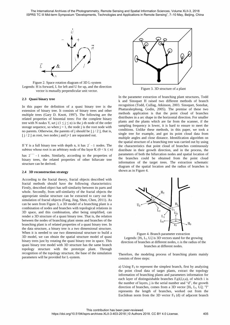
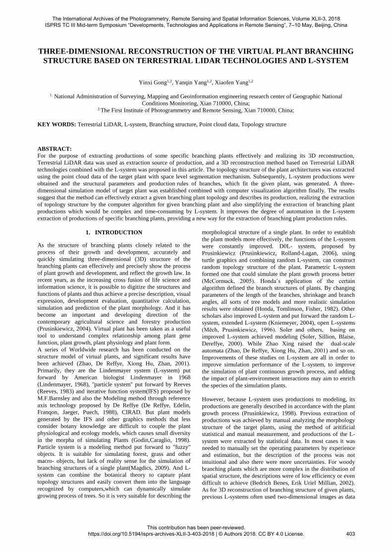
Figure 2. Space rotation diagram of 3D L-system

Legends: H is forward, L for left and U for up, and the direction

vector is mutually perpendicular unit vector.

2.3 Quasi binary tree

In this paper the definition of a quasi binary tree is the

extension of binary tree. It consists of binary trees and other

multiple trees (Gary D. Knott, 1997). The following are the

related properties of binomial trees: For the complete binary

tree with N nodes Y, set j (1 ≤ j ≤ n) is the j-th node of the order

storage sequence, so when j = 1, the node j is the root node with

no parents. Otherwise, the parents of j should be ⌊ j / 2 ⌋, that is,

⌊ j / 2 ⌋ as root, two nodes j and j+1 are separated out.

If Y is a full binary tree with depth n, it has 2 1n

nodes. The

subtree whose root is an arbitrary node of the layer K (0 < k ≤ n)

has k 1

2 1n

nodes. Similarly, according to the properties of

binary trees, the related properties of other bifurcate tree

structure can be derived.

2.4 3D reconstruction strategy

According to the fractal theory, fractal objects described with

fractal methods should have the following characteristics:

Firstly, described object has self-similarity between its parts and

whole. Secondly, from self-similarity of the fractal objects the

appropriate similar structure can be extracted to carry out the

simulation of fractal objects (Fang, Jing, Shen, Chen, 2011). As

can be seen from Figure 3, a 3D model of a branching plant is a

combination of nodes and branches with topological relations in

3D space, and this combination, after being simplified, can

render a 3D structure of a quasi binary tree. That is, the relation

between the nodes of branching plant stems and branches of the

branching plant is of related properties of a quasi binary tree. In

the data structure, a binary tree is a two dimensional structure.

When it is needed to use two dimensional structure to build a

3D model, we can obtain the spatial structure model of quasi

binary trees just by rotating the quasi binary tree in space. This

quasi binary tree model with 3D structure has the same branch

topology structure with the prototype plant. Through

recognition of the topology structure, the base of the simulation

parameters will be provided for L-system.

Figure 3. 3D structure of a plant

In the parameter extraction of branching plant structures, Todd

k and Sinoquet H raised two different methods of branch

recognition (Todd, Csillag, Atkinson, 2003. Sinoquet, Sonohat,

Phattaralerphong, Godin, 2005). The premise of these two

methods application is that the point cloud of branches

distributes in a arc shape in the horizontal direction. For smaller

plants and the plants which are far from the scanner, if the

sampling frequency is lower, it is hard to ensure to meet the

conditions. Unlike these methods, in this paper, we took a

single tree for example, and got its point cloud data from

multiple angles and close distance. Identification algorithm on

the spatial structure of a branching tree was carried out by using

the characteristics that point cloud of branches continuously

distribute in their growth direction, and in the process, the

parameters of both the bifurcation nodes and spatial location of

the branches could be obtained from the point cloud

information of the target trees. The extraction schematic

diagram of the spatial location and the radius of branches is

shown as in Figure 4.

Figure 4. Branch parameter extraction

Legends: [Hi, Li, Ui] is 3D vectors stand for the growing

direction of branches at different nodes, ri is the radius of the

branches at different nodes.

Therefore, the modeling process of branching plants mainly

consists of three steps:

a) Using Fij to represent the simplest branch, first by analyzing

the point cloud data of target plants, extract the topology

information of branching plants and parameters information for

each layer of distinguishable branches Fij(d,l,r,a), of which i is

the number of layers, j is the serial number and “d”, the growth

direction of branches, comes from a 3D vector [Hi, Li, Ui]; "l"

represents the length of branches, worked out from the

Euclidean norm from the 3D vector Fij (d) of adjacent branch



405

node and Fi+1j(d), its formula is as follows: , 1 ,

l F Fi j i j

; “r” is

the radius of the drawn branches, extracting from the formula

r / 2C , in which C is the perimeter of the contours of the

point cloud cross-section fitting; "a" represents the attenuation

coefficient of the branches, resulted from the formula

ij 1 , ,F (a) F (r) / F (r)

i j i j , in which Fij(r) is the branch radius at the

node of the adjacent branches.

b) Then through generalizing and abstracting the structures

combined with the characteristic parameters of branching plants,

form the axiom (the starting strings) and production rules, and

further iteratively generate a character sequence representing

tree structures.

c) Finally translate each character in the L-system into

corresponding graphic elements, and combining with the

already extracted production rules as well as using 3D L-system,

achieve the goal of 3D reconstruction of target plants.

2.5 Extraction algorithm of branching plant topology

structure based on point cloud data

From the view of biology, growing and developing of plants is a

natural process of continuous changes (Godin, Sinoquet, 2005).

So we can think the spatial location of the barycenter of the

same structure in the continuous cross-section is of continuous

change. That is to say, their trajectories in space are a set of line

segments of geometric continuity.

On the basis of the theory above, according to the spatial

structures of branching plant, in this article we propose a

topology extraction algorithm of branching plant based on

barycenter. In the algorithm, space is firstly divided into

hierarchical grids, and the point cloud on each grid is projected

onto a two-dimensional plane. Using fitting method, the discrete

point cloud data is fitted into two-dimensional graphics with

polygon boundary; Then, through computer graphic analysis,

the cross-section of branching plant is formed; Finally, by

detecting the continuous distribution of barycenter of faults in

vertical direction, the topology structures of the branching plant

are reconstructed. Thus, we can accurately determine the spatial

locations of plant stems, geometric shapes and the spatial

relationships between the stems, and thus we get the topology

structures of branching plant. The following are the topology

structure of branching plant of this case, as shown in Figure 5,

which corresponds to the adjacent lists of node to node, branch

to branch, shown in table 1, table 2.

Node Parent Child Coordinate (x, y,

z)

Radius

(r)

N11 - N21 N11(x, y, z) N11(r)

N21 N11 N31, N32,

N33 N21(x, y, z) N21(r)

N31 N21 N41 N31(x, y, z) N31(r)

N32 N21 - N32(x, y, z) N32(r)

N33 N21 N42, N43 N33(x, y, z) N33(r)

N41 N31 N51, N52,

N53 N41(x, y, z) N41(r)

N42 N33 - N42(x, y, z) N42(r)

N43 N33 N54 N43(x, y, z) N43(r)

N51 N41 - N51(x, y, z) N51(r)

N52 N41 - N52(x, y, z) N52(r)

N53 N41 - N53(x, y, z) N53(r)

N54 N43 - N54(x, y, z) N54(r)

Table 1. Adjacency lists of the node-node topology relationship

Note: Where Nij (x, y, z) is the node coordinates, Nij (r) is

branch radius at the nodes

Figure 5. Topology example of branch segments - node

Legends: Nij is nodes, Lij is branch segments.

Branch Parent Child

L11 - L21, L22, L23

L21 L11 L31

L22 L11 -

L23 L11 L32, L33

L31 L21 L41,L42, L43

L32 L23 -

L33 L23 L44

L41 L31 -

L42 L31 -

L43 L31 -

L44 L33 -

Table 2. Adjacency lists of the segment-segment topology

relationship of branches

Note: Where Lij is branch segments.

Extended with the node N11 as the starting point, the resulting

adjacent lists of topological relationship of the branch segment-

node are shown in Table 3.

Branch Start point End point Length

L11 N11 N21 L11( l )

L21 N21 N31 L21( l )

L22 N21 N32 L22( l )

L23 N11 N33 L23( l )

L31 N21 N41 L31( l )

L32 N23 N42 L32( l )

L33 N23 N43 L33( l )

L41 N31 N51 L41( l )

L42 N31 N52 L42( l )

L43 N31 N53 L43( l )

L44 N33 N54 L44( l )

Table 3. Adjacency lists of the segment-node topological

relation

From the topology relations above, the parameter information of

each segment of branches can be obtained. Take extracting the

parameters of the segment F11(d,l,r,a) as an example, the branch

segment belonging to F11 is L11, so F11 gets the topology

information of L11. Therefore the starting point coordinate of F11

(d ) is N11 (x, y, z), the end point coordinate is N21(x, y, z) and

the 3D vector [ H11 , L11, U11 ] can be obtained by the two



406

http://dict.cnki.net/dict_result.aspx?searchword=%e5%9d%90%e6%a0%87&tjType=sentence&style=&t=coordinate

coordinates; F11 (l) is equal to L11(l); F11(r) is equal to N11(r);

and F11(a) can be resulted from the ratio of 21 11

F (r) / F (r) . Thus

all the parameter information in the F11(d, l, r, a) can be

obtained.

The following is the specific extraction process of the algorithm:

Step1: Read the point cloud data of target plants, namely the

trees needing 3D reconstruction.

Step2: Extract the point clouds of fault trees at certain intervals

and thicknesses (the interval and thickness are based on the

complexity of the trees), and the numbers are adjacent between

the faults.

Step3: Project the point clouds of each fault to a plane vertically

and respectively, and then use the quadratic Laplacian to

exclude discrete noise points (Felsberg, Sommer, 2001),

excluding the interference of leaves and small branches, and

making the stems and main branches the remaining parts;

Step4: Form one or more two-dimensional graphics with closed

polygons by fitting the projection graphics in Step3, and extract

the contours of branchs. As shown in figure 6 a shows;

Step5: use P.Guldin theorem (Yang, 2004) to work out the

barycenters for all the closed two-dimensional graphics of each

fault, extract the barycenters of branches and stems. As shown

in figure 6b.

Figure 6. Branch contour fitting and extraction of barycenters

Legends: The red points represent the barycenter, and blue

segments are the growth direction of branches.

Step6: After connecting the barycenters of branches between

each adjacent layer through line segments, we actually get the

spatial locations of nodes on each branch layer, radius ri of each

branch segment and also the spatial location of each branch

represented by the three vectors [Hi, Li, Ui] in the 3D L-system,

and accordingly get a topology structure of the prototype tree

branches, as shown in Figure 7;

Figure 7. Extraction of the spatial location and radius of

branches

Legends: ri is each branch segment radius, [Hi, Li, Ui] is three

vectors of each branch direction, Ni is number of each adjacent

layer.

Step7: Following the topology of tree branches, extract the type

of branches, make adjustments to the structure models of

branches, integrate the branching structures of various types,

and build the corresponding structure models of quasi binary

trees. In this article we define Y is the binary branch, and K the

three forks branch;

Step8: Simplify the topology models of tree branches, until the

most simple branches, shown in Figure 8;

Figure 8. Simplification process and iterative rules of branches

structure

Step9: Extract the iteration number n and the type and the

parameters of each branch according to the topology model of

prototype trees in Step6, and establish character tables of the

simplest branches of various types, including the length l of

each simplest branches, radius r of branches, and other key

elements as growth direction d;

Step10: Determine the basic iteration rules of Y, K and axioms

ω of all kinds of branches;

Step11: According to the character table of the most simple

branches, perfect the basic iteration rules, establish a complete

production, and thereby establish a complete L-system model.

2.6 Branch reconstruction based on L-system

On the proposed method above, some related indexes can be

obtained: branch type Bt, physiological cycle (called the

iteration number) n of plant growth and the morphological

structure of plants, and production for extraction L-system

modeling. And according to the nature of quasi binary trees of

branching plants, branching number ( 1)

2 1 nnum

, node



407

dict://key.0895DFE8DB67F9409DB285590D870EDD/topological%20structure

number

i 1

Nod i

n

n imun

,in which 1 n bt , i

mun is

the number of different branches, namely the product of each

different branching type and the branch. Therefore, the L-

system based on the method in this paper can be defined as:

1) ω: the minimalist branches

2) Iteration number n: the layer number n of the topology

structure of plants

3) Production p: first, determine the basic production of each

branching type, according to the number Bt of branch types,

such as binary branches [Y] [Y], three forks branch [K] [K] [K],

and then according to the 3D coordinates of the nodes of each

layer in the topology structure of plants, said with 3D L-system

vectors [H, L, U], and combining with the most simple branches

of the layers which contain the information of branch length "l",

branch radius "r" as well as the attenuation coefficient "a" of the

branches, thus establish reasonable production which is

consistent with the prototype trees.

By the process of the production description, the structure and

number of production p is decided by the branching structure

and spatial location of nodes of each layer. Their numbers can

be expressed as:

1 *

iBt p 2 1 i R

n

( ) (1)

That is, the more branch types Bt and the branch number, the

more the production Pi the greater the total number of growth

units S, and the more complex the generated 3D structures of

plants.

Because the production description of L-system is closely

related with the growing process of plants (Pradal, Dufour-

Kowalski, Boudon, Fournier, Godin, 2008), and both the

production number and the structure description are of

uncertainty (Federl, Prusinkiewicz, 2004), the following

relation exists between the number of productions and branch

types Bt:

*

iBt p i R （） (2)

From the comparison of (1), (2) and the describing process of

production p in this paper, in production number and the

description for each rule, the method in this article has strong

operability with certainty.

3. RESULTS AND DISCUSSION

Using C++ in the Visual Studio 2008, in this article we have

studied and developed the simulation system for 3D structure

reconstruction of branching plants by Terrestrial LiDAR data.

The defined data structure in the research and the codes of the

related main program are as follows:

Typedef struct TreeNode

{

unsigned Index;

char Axiom; // Axiom

int Layers; // Iteration times

char Rule[num]; // Production ruls

char Bt[n]; // Branch types

float Direction[n]; // The direction vectors of branches in space

}

void CTreeView::Draw()

{

InitDatas(); // Initialized data

void (*p)(); // Define pointer variables to a function

p=E; //The entry address of a function of recording

information passing

ConstructTree(); // Construct plant production

DrawTree() ; // Reconstruct 3D shapes of plants according to

the productions

}

In the process of reconstruction, first analyze the detached point

cloud information of prototype tree, and extract the parameter

information of topology structures of the tree and identifiable

branches. And then by generalization and abstraction of the

topology and parameters and building production rules,

progressively and iteratively generates a character sequence of

the tree structure. Finally, each character in the L-system is

interpreted into corresponding graphic elements, and using the

3D L-system, 3D reconstruction of trees is realized. The

simulation results are shown in Figure 9 and Figure 10.

Figure 9. Simulation results of an Oak

Legends: a) Scene photographs of the Oak prototype. b) Point

cloud screenshot of the Oak prototype. c) Simulation result

Figure 10. Simulation results of a Locust

Legends: a) Scene photo of the Locust prototype. b) Point cloud

Screenshot of the Locust prototype. c) Simulation results

In Fig. 9 and 10, the results of the 3D reconstruction of trees

show that the models of trees constructed by the method

proposed in this article are highly consistent with the prototype

trees. Most branches have achieved reasonable reconstruction

effects, and expressions of the main branches are correct. The

3D reconstruction of the branching plants has been achieved.

But it can also be seen that the simulation results still need to be

improved. Taking c) in figure 10 for example, we can clearly see

that not all branches have been reconstructed, and that some

smaller branches have not been presented or the expressions are

incomplete. This is due to the reasons that the dense leaves

shade, that the branches are too small, and also that the branch

growth is more irregular, causing the branches to be filtered out

by denoising algorithm or fail to pass the algorithm

identification. For this kind of problems, we are considering to

resolve by means of improving the topology extraction

algorithm or manual intervention in future studies, but the

manual intervention will reduce automation degree the method



408

proposed in this paper.

And it can also be found from c) in fig. 9 and c) in fig. 10 that

branches of the trees did not show the natural shape of curve.

This is because the geometry models of branches in the parser

uses a round platform, and so it is difficult to simulate the

branches with curvature. In the further study generalized

cylinder will be used in the geometric expression of branches,

and thus the branches in the form of curve can be simulated.

Due to accidental errors of the field data, parts of the point

cloud data of the target plants require artificial corrective

treatment, with which the 3D reconstruction of trees can be of

better results. In this paper, in the future research we will

consider the introduction of the method of smooth fitting of the

point cloud, which will make the method in this article more

automating.

Sample data of the simulation plant as shown in table 4,

simulation results show that this method can effectively use 3D

Terrestrial LiDAR data to describe the production of given

plants which is consistent with the reality, and has good

practicality.

Target

trees

Branch

number

Layer

number

Total

number

of

nodes

Number

of

growth

units

Number of

productions

Oak 105

（127） 8 232 1376 12

Locust 35

（63） 7 91 2365 8

Table 4. Experimental data

4. CONCLUSION

On the base of the study on the characteristics of Terrestrial

LiDAR data as well as 3D L-system, we present a 3D

reconstruction method of branching structures of given plants

based on the Terrestrial LiDAR data combined with L-system.

Simulation results show that this method effectively obtained

branching structures which consistent with the real ones of

given plants and realized 3D reconstruction of their branches.

Using algorithms to extract the topology structures of plants and

then extract the characteristics of production, the previous L-

system has been improved, while it relied on the method of a

large number of experimental observation and analysis of

statistics in the extraction of plant production which was time-

consuming, complex and uncertain.

Terrestrial LiDAR technology has been repeatedly applied in

the extraction of geometrical and biological parameters of

individual plant, but due to the complexity of the spatial

structures of plants and the incompleteness of point cloud data,

most results were not accurate and ideal enough. This article

used Terrestrial LiDAR system with high spatial resolution,

using close and multi-station way to obtain the complete point

cloud information of the target plants, and thus remedying the

shortcomings above, achieved a good data base. On the basis of

complete point cloud data of the target plants, the space-level

segmentation mechanism presented in this paper can better

extract the spatial topology information and branch parameters

of the target plants, achieving an automatic extraction of

topology structures of plants by using computer algorithm.

Following the steps in this paper, through establishing

algorithm to analyze the plant topology and then extracting the

production, even the persons who is not very familiar with the

L-system can also use the method to extract the production of

plants and generate 3D models with high degree of simulation,

improving the efficiency of the extraction of plant production

and providing a basis for the study of the physiological and

ecological processes related to plant structures, and also

providing a new way for the description of plant production.

However, due to the complexity of the growing structures of

plants, while extracting small branches and winding branches

using the method, the results were less than ideal, and there

were slightly differences between the simulation results and the

original structures of plants, but that does not affect the

applicability of this method. Future research following this

article will focus on improving the method of parameters

information extraction of the branching structure of plants by

Terrestrial LiDAR data, to make it possible to identify more

complex branches, to extract the correct plant production and to

establish plant models which are consistent with reality.

In the future work it is needed to consider how to simulate the

dynamic growth of a given plant by using plant leaves

combined with the growing function in the scale of time, so as

to make predictions and retrieval on growing processes of it.

ACKNOWLEDGEMENTS

Financial support for this study was provided through National

Key Technology R&D Program (2014BAH34B01). We are

grateful to the undergraduate students and staff of the

Laboratory of Forest Management and “3S” technology, Beijing

Forestry University, and the great support from Beijing

Municipal Bureau of Forest. A special thank is due to LI, from

Tsinghua University for careful revision of English text.

REFERENCES

Bedrich Benes, Erik Uriel Millian. (2002). Virtual climbing

plants competing for space. Proceedings of the Computer

Animation 2002. Geneva, Switzerland. 19- 21(6), pp. 33-43.

Bian, R., Chen, P., Burrage, K., Hanan, J., Room, P., & Belward,

J., (2002). Derivation of L-system models from measurements

of biological branching structures using genetic algorithms.

Lecture Notes in Computer Science. 2358, pp. 514-524.

Christophe Godin, Hervé Sinoquet. (2005). Functional-

structural plant modeling. New Phytologist. 166(3), pp. 705-708.

De Reffye, P., Edelin, C., Franqon, J., Jaeger, M., & Puech, C.

(1988). Plant models faithful to botanical structure and

development. Computer Graphics. 22(4), pp. 151-158.

Doron Rotem & Varol, Y. L. (1978). Generation of Binary Trees

from Ballot Sequences. Journal of the ACM (JACM). pp. 396 –

404.

Fang, K., Jing, S., Shen, L. M., & Chen, y. (2011). Three-

dimensional reconstruction of virtual plants branch structure

based on quasi binary-tree. Transactions of the CSAE, 27(11),

pp. 151-154.

Federl, P., & Prusinkiewicz, P. (2004). Solving differential

equations in developmental models of multicellular structures

expressed using L-systems. Lecture Notes in Computer Science.



409

dict://key.0895DFE8DB67F9409DB285590D870EDD/round%20platform

pp. 3037, 65-72.

Felsberg, M., & Sommer, G. (2001). Scale Adaptive Filtering

Derived from the Laplace Equation. Pattern Recogniton.

Lecture Notes in Computer Science. pp. 124-131.

Fujita, M., McGeer, P.C., & Yang, J. C. Y. (2005). Multi-

Terminal Binary Decision Diagrams: An Efficient Data

Structure for Matrix Representation. FORMAL METHODS IN

SYSTEM DESIGN. pp. 149-169.

Gary D. Knott. (1997). A numbering system for binary trees.

Communications of the ACM. pp. 113-115.

Garber, S. M., Monserud, R. A., & Mguire, D. A. (2008).

Crown recession patterns in three conifer species of the

Northern Rocky Mountains. Forest Science. 54(6), pp. 633-646.

Godin,C., & Caraglio, Y. (1998). A multiscale model of Plant

topological structures. Journal of Theoretical Biology. 19(1), pp.

l-46.

Godin, C., & Sinoquet, H. (2005). Functional–structural plant

modelling. New Phytol. 166(3), pp. 705-708.

Gorte, B., & Pfeifer, N. (2004). Structuring laser-scanned trees

using 3d mathematical morphology. Proceedings of

Commission V, Istanbul, Turkey. pp. 929-933.

Honda, H., Tomlinson, P. B., & Fisher, J. B. (1982). Two

geometrical models of branching of botanical trees. Annals of

Botany. 49, pp. l-11.

Hu, B. G., De Reffye, P., Zhao, X., Yan, H. P., & Kang, M. Z.

(2003). GreenLab: towards a new methodology of plant

structural functional model structural aspect. Tsinghua

University Press. pp. 21-35.

Jean-Louis Loday., & María O. Ronco. (2002). Order Structure

on the Algebra of Permutations and of Planar Binary Trees.

JOURNAL OF ALGEBRAIC COMBINATORICS. pp. 253-270.

Karwowski, R., & Prusinkiewicz, P. (2003). Design and

implementation of the L+C modeling language. Electronic

Notes in Theoretical Computer Science. 86, 19.

Kniemeyer, O. (2004). Rule-based modelling with the

XL/GroIMP software.In: Schaub H, Detje F, Brüggemann U,

eds. The logic of Artificial Life. Proceedings of the 6th GWAL.

Berlin: AKA Akademische Verlagsgesellschaft, pp. 56-65.

Lacointe, A., Isebrands, J. G., & Host, G. E. (2002). A new way

to account for the effect of source–sink spatial relationships in

whole plant carbon allocation models. Canadian Journal of

Forest Research. 32, pp. 1838-1848.

Lindenmayer, A. (1968). Mathematical models for cellular

interaction in development, PartsⅠand Parts Ⅱ . Journal of

Theoretical Biology. 19, pp. 280-315.

Liu, Y. L., Wang, J., Chen, X., Guo, Y. W., & Peng, Q. S. (2008).

A Robust and Fast Non-Local Means Algorithm for Image

Denoising. COMPUTER SCIENCE. JOURNAL OF

COMPUTER SCIENCE AND TECHNOLOGY. pp. 270-279.

Magdics, M. (2009). Real-time generation of l-system scene

models for rendering and interaction. Spring conference on

computer graphics. Comenius University. pp. 77-84.

McCormack, J. (2005). Aesthetic evolution of L-systems

revisited. Applications of Evolutionary Computing. pp. 475-486.

Měch, R., & Prusinkiewicz, P. (1996). Visual models of plants

interacting with their environment. Proceedings of SIGGRAPH

96, New Orleans, LA, 4-9 August 1996. ACM SIGGRAPH, pp.

397-410.

Omasa, K., Hosoi, F., & Konishi, A. (2007). 3D LiDAR

imaging for detecting and understanding plant responses and

canopy structure. Journal of experimental botany. 58(4), pp.

881-898.

Parker, G. G., Harding, D. J., & Berger, M. L. (2004). A portable

LiDAR system for rapid determination of forest canopy

structure. Journal of Applied Ecology. 41, pp. 755-767.

Pradal, C., Dufour-Kowalski, S., Boudon, F., Fournier, C., &

Godin, C. (2008). OpenAlea: a visual programming and

component-based software platform for plant modelling.

Functional Plant Biology. 35, pp. 751-760.

Prusinkiewicz, P. (1998). Modeling of spatial structure and

development of plants. Scientia Horticulturae. 74, pp. 113-149.

Prusinkiewicz, P. (2004). Art and science for life: designing and

growing virtual plants with L-Systems. Acta Horticulturae. 630,

pp. 15-28.

Prusinkiewicz, Z. (2004). Modeling plant growth and

development. Current Opinion in Plant Biology. 7(1), pp. 79-83.

Prusinkiewicz, P., & Rolland-Lagan, A. G. (2006). Modeling

plant morphogenesis. Current Opinion in Plant Biology. 9, pp.

83-88.

Rakocevic, M., Sinoquet, H., & Christophe, A. (2000).

Assessing the geometric structure of a white clover canopy

using 3-D digitising. Annals of Botany. 86, pp. 519-526.

Reeves, W. T. (1983). Particle systems-A technique for

modeling a class of fuzzy objects. Computer Graphics. 17(3),

pp. 359-376.

Shlyakhter, I., Rozenoer, M.., Dorsey, J., & Teller, S. (2001).

Reconstructing 3D tree models from instrumented photographs.

Computer Graphics and Applications. 21 (3), pp. 53-61.

Sinoquet, H.., Sonohat, G., Phattaralerphong, J., & Godin, C.

(2005). Foliage randomness and light interception in 3-D

digitized trees: an analysis from multiscale discretization of the

canopy. Plant, Cell and Environment. 28(9), pp. 1158-1170.

Todd, K., Csillag, F., & Atkinson, P. M. (2003). Three-

dimensional mapping of light transmittance and foliage

distribution using LiDAR. Canadian Journal of Remote

Sensing. 29(5), pp. 544-555.



410

THREE-DIMENSIONAL RECONSTRUCTION OF THE VIRTUAL PLANT ...

Documents

Transcript of THREE-DIMENSIONAL RECONSTRUCTION OF THE VIRTUAL PLANT ...