Three Dimensional Radiation Hydrodynamics Simulations of Core...
14
Three Dimensional Radiation Hydrodynamics Simulations of Core Collapse Supernovae Luke F. Roberts TAPIR, Caltech
Transcript of Three Dimensional Radiation Hydrodynamics Simulations of Core...
ThreeDimensionalRadiationHydrodynamicsSimulationsofCoreCollapseSupernovae
LukeF.RobertsTAPIR,Caltech

CoreCollapseSupernovae:Multi-messengerevents
2
Energy
(MeV
)
Time(s)
SeeBiontaetal.’87andHirataetal.‘87
Neutrinos
GravitationalWaves
FromOttetal.‘12
Electromagnetic
FromFilppenko‘97
Nucleosynthesis
FromAmarsietal.‘15
L4 A. M. Amarsi, M. Asplund, R. Collet, and J. Leenaarts
−0.5
0.0
0.5
1.0
1.5
−0.5
0.0
0.5
1.0
1.5
[O/F
e]
[OI] 630nmOI 777nm
−3 −2 −1 0[Fe/H]
−1.0
−0.5
0.0
0.5
1.0
[O/F
e]63
0−[O
/Fe]
777
Figure 3. Final results based on equivalent widths from the lit-erature (Carretta et al. 2000; Fulbright & Johnson 2003; Bensbyet al. 2004; Akerman et al. 2004; Garcıa Perez et al. 2006; Fabbianet al. 2009; Nissen et al. 2002, 2014; Bertran de Lis et al. 2015)and stellar parameters from Nissen et al. (2014) and Casagrandeet al. (2010, 2011). Top: [O/Fe] vs [Fe/H] inferred from the[OI] 630 nm line (red circles) and from the OI 777 nm lines (blackdiamonds). Lines of best fit to the data in the domains �2.5 <[Fe/H] < �1.0 and �1.0 < [Fe/H] < 0.0 are overdrawn. The fitswere obtained by minimising �2 and assigning each star equalweight; where abundances from both diagnostics were available,the mean value was used. Bottom: di↵erences in [O/Fe] for indi-vidual stars inferred from the [OI] 630 nm and OI 777 nm lines,for the cases where both sets of equivalent widths were avail-able. The median value is 0.02 dex and the standard deviation is0.14 dex.
Lyman-↵ line provides an e�cient alternative destructionroute for UV photons at low [Fe/H] that completely stiflesthe photon pumping e↵ect in the OI 130 nm lines. Thus, inthe absence of an alternative non-LTE mechanism, we areleft with small departures from LTE in the OI 777 nm linesat low [Fe/H].
4 THE GALACTIC CHEMICAL EVOLUTIONOF OXYGEN
The equivalent widths of the [OI] 630 nm andOI 777 nm lines were taken from a number of studiesof dwarfs and subgiants based on high signal-to-noiseobservations (Carretta et al. 2000; Fulbright & Johnson2003; Bensby et al. 2004; Akerman et al. 2004; Garcıa Perezet al. 2006; Fabbian et al. 2009; Nissen et al. 2002, 2014;Bertran de Lis et al. 2015). Where more than one valuewas available for a given star and line, the unweightedmean was adopted. For consistency, equivalent widthsacross the theoretical 3D non-LTE grid were computed byfitting Gaussian functions to the line fluxes and integratinganalytically. Stellar parameters were taken from severalrecent studies (Casagrande et al. 2010, 2011; Nissen et al.2014). These Te↵ estimates were either derived using orcritically compared to the accurate IRFM calibrations of
Casagrande et al. (2010); where more than one set of stellarparameters was available for a given star, the newest setwas adopted.
Hitherto, studies have typically found discrepant resultsfrom the two abundance diagnostics at low [Fe/H] (§1).In Fig. 3 we compare the [O/Fe] ratios inferred from ouranalyses. We have found the [OI] 630 nm line and theOI 777 nm lines to give similar [O/Fe] vs [Fe/H] trendsdown to [Fe/H] ⇡ �2.2, the lowest metallicity in which the[OI] 630 nm line is detectable in halo subgiants and turn-o↵stars. Furthermore, the abundances inferred from these di-agnostics in the atmospheres of the same stars are consistentto within a standard deviation of 0.14 dex.
It bears repeating that there are two factors in our anal-ysis that are absent in most previous studies, that conspireto give concordant results between the two abundance di-agnostics. First, we have accounted for 3D non-LTE e↵ectsin the OI 777 nm lines: these are of decreasing importancetowards lower [Fe/H] , but even then remain significant. Sec-ond, we have used new and accurate stellar parameters: themore reliable IRFM calibrations give Te↵ estimates that aresignificantly larger than those typically used in the past.
The [O/Fe] vs [Fe/H] relationship in Fig. 3 reflects theevolution with time of oxygen and iron yields. Oxygen is syn-thesised almost entirely in massive stars (M & 8M�), itsmost abundant isotope 16O being the endpoint of Heliumburning (Woosley et al. 2002; Clayton 2003; Meyer et al.2008). Since iron is synthesised in type II supernovae ex-plosions (Woosley et al. 2002), the plateau at [O/Fe] ⇡ 0.5between �2.2 . [Fe/H] . �1.0 indicates that massive starsat this epoch eject an approximately constant ratio of oxy-gen and iron upon their deaths, in agreement with Galacticchemical evolution models (Francois et al. 2004; Kobayashiet al. 2006). The steep linear decay seen above [Fe/H] & �1.0is usually interpreted as a sign of the long-lived type Iasupernovae becoming significant, increasing the rate of en-richment of iron into the cosmos (Tinsley 1979; McWilliam1997).
At [Fe/H] . �2.5 there is a slight upturn in [O/Fe],but it is less pronounced than found from the 1D LTE anal-yses of OH UV lines by Israelian et al. (1998, 2001) andBoesgaard et al. (1999). The upturn could indicate a shiftin the mass distribution of stars at earlier epochs; stars thatare more massive and more metal-poor are expected to yieldlarger oxygen-to-iron ratios (Kobayashi et al. 2006). We cau-tion however that inferences in this region are less reliablebecause they are based on a very small sample of stars andon analyses of the OI 777 nm lines alone. A larger sampleof halo turn-o↵ stars with accurate stellar parameters andvery high signal-to-noise spectra will be needed to confirmthis result.
ACKNOWLEDGEMENTS
AMA and MA are supported by the Australian ResearchCouncil (ARC) grant FL110100012. RC acknowledges sup-port from the ARC through DECRA grant DE120102940.This research has made use of the SIMBAD database, op-erated at CDS, Strasbourg, France. This research was un-dertaken with the assistance of resources from the National
MNRAS 000, 1–5 (—)

CoreCollapse
€
GMNS2
RNS
~ 3×1053 erg
▪StarswithM>~9MsunburntheircoretoFe
▪CoreexceedsaChandrasekharmasssupersoniccollapseoutsideofhomologouscorebounceshockafter~2xsaturationdensity
▪Gravitationalbindingenergyofcompactremnant:
€
~ 1051erg
▪Bindingenergyofstellarenvelope:
▪NoExplosionsbytheneutrinomechanisminsphericalsymmetry(e.g.Liebendorfer’00)
0
10
20
30
40
L n(1
052er
gs�
1 )
�100 �50 0 50 100 150 200Time Post Bounce (ms)
68
10121416
e
n
(MeV
)

PostBounceEvolutionofCCSNe
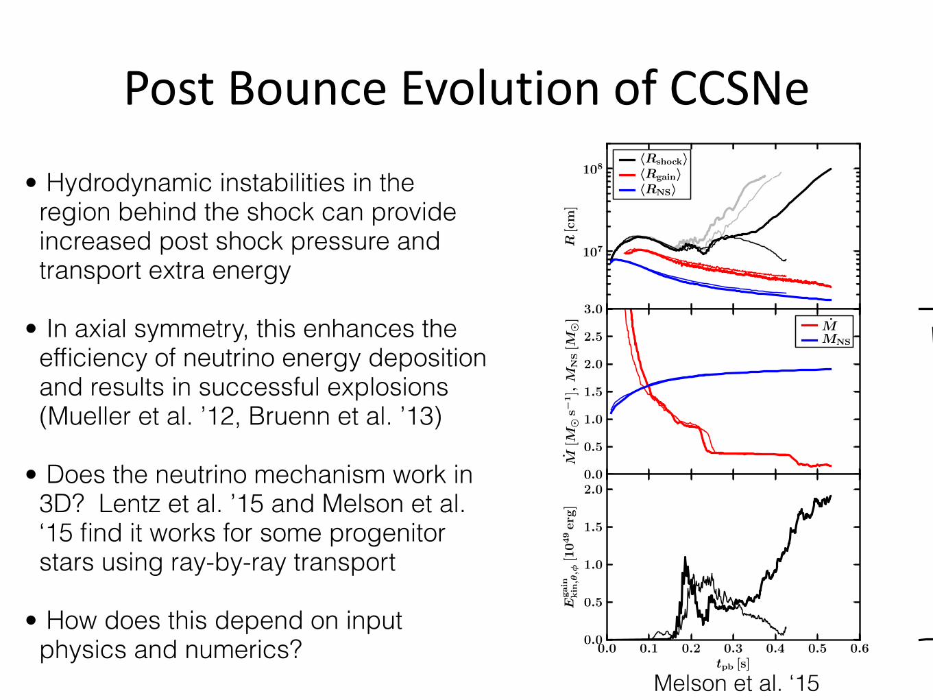
• Hydrodynamic instabilities in the region behind the shock can provide increased post shock pressure and transport extra energy
• In axial symmetry, this enhances the efficiency of neutrino energy deposition and results in successful explosions (Mueller et al. ’12, Bruenn et al. ’13)
• Does the neutrino mechanism work in 3D? Lentz et al. ’15 and Melson et al. ‘15 find it works for some progenitor stars using ray-by-ray transport
• How does this depend on input physics and numerics?

PostBounceEvolutionofCCSNe
Instability Regimes in Collapsing Stellar Cores 3
0 0.05 0.1 0.15 0.2time after bounce [s]
0
100
200
300
400
500
600
700
800
900
1000
min
., m
ax., a
vg. sh
ock
rad
ius
s27.0u8.1
Figure 2. Maximum, minimum (solid lines) and average (dashedlines) shock radius for model s27.0 (black lines) and u8.1 (red).
genitors, and is dramatically different from stars even afew tenths of a solar mass more massive. The density pro-file more closely resembles an asymptotic giant branch(AGB) star, or an electron-capture supernova progeni-tor, than a typical massive star structure in that it has alow-density “envelope” (ρ < 1 g cm−3) directly on top ofa dense core (ρ > 106 g cm−3) of 1.38M⊙, with a tran-sition region of only 0.03M⊙, mostly the carbon layer,in between. Outside the 1.26M⊙ iron core are layers ofsilicon (out to 1.30M⊙), oxygen (to 1.36M⊙), neon, andcarbon, with implosive energy generation due to silicon,oxygen, and neon burning as high as 1017 erg g−1 s−1.Note that the structure of model u8.1 is specific to suchlow-mass supernova progenitors, and not owing to theinitial metallicity of the model; a different initial metal-licity would only change the location and extent of themass range between the AGB channel and the “normal”channel of iron core evolution familiar from more massivestars.Model s27.0, by contrast, has a more massive and less
compact iron core of 1.5M⊙ embedded in a thick siliconshell that reaches out to 1.68M⊙, where the transition tothe oxygen-enriched silicon shell is located. Comparedto model u8.1, the density drops far less rapidly outsidethe iron core. In order to better illustrate the differentdensity structure of the two models, we show densityprofiles of the progenitors in Figure 1.We use a numerical grid of nr × nθ = 400× 128 zones
with non-equidistant radial spacing for both progeni-tors. Model s27.0 was simulated using the equation ofstate (EoS) of Lattimer & Swesty (1991) with a valuefor the bulk incompressibility modulus of nuclear matterof K = 220 MeV (LS220), while the softer variant withK = 180 MeV (LS180) was chosen for model u8.1. Fora discussion of the validity of the latter EoS for small-mass (baryonic mass ! 1.5M⊙) proto-neutron stars de-spite its marginal inconsistency with the 1.97M⊙ neutronstar found by Demorest et al. (2010), see Muller et al.(2012). Specifically, the mass-radius relation for hot andcold neutron stars is very similar for neutron stars wellbelow the mass limit. As a consquence, both equationsof state yield hardly any difference during the accretionphase (Swesty et al. 1994; Thompson et al. 2003).
3. RESULTS
Superficially, model s27.0 and u8.1 might appear toevolve in a very similar fashion: Roughly around 120 ms
0.05 0.1 0.15 0.2time after bounce [s]
0
0.2
0.4
0.6
0.8
1
1.2
1.4
1.6
1.8
2
2.2
2.4
τad
v/τ
hea
t
s27.0u8.1
Figure 3. The runaway criterion τadv/τheat for model s27.0(black) and model u8.1 (red). Both τadv and τheat are evaluated asin Muller et al. (2012). Note that the curves have been smoothedusing a running average over 5 ms.
after bounce the average shock radius starts to increase,and by 200 ms the shock is already expanding rapidly,although model s27.0 evidently lags behind u8.1 a little(Figure 2). Especially during the later phases, the shockbecomes strongly deformed with a ratio rmax/rmin of themaximum and minimum shock radius on the order of2 . . . 3. Both models seems to provide similar examplesfor an explosion at a relatively early stage.However, this appearance is deceptive: A hint at
more profound differences between s27.0 and u8.1 is al-ready furnished by the critical ratio τadv/τheat of the“advection” or “residence” time-scale and the heatingtime-scale for the material in the gain region, whichserves as an indicator for an explosive runaway dueto neutrino energy deposition (for τadv/τheat > 1; seeJanka 2001; Thompson et al. 2005; Buras et al. 2006a;Murphy & Burrows 2008; Fernandez 2012). Figure 3shows that model s27.0 approaches the critical thresh-old much later than model u8.1, i.e. at roughly ∼180 msinstead of ∼110 ms. Nevertheless, even though the run-away condition is not yet met, the shock already expandsconsiderably before that time in model s27.0. This sug-gests that at least for the first ∼180 ms there may be adriving agent other than neutrino heating that is respon-sible for pushing the shock outwards. One should bear inmind, however, that it is not completely clear for whichvalue of τadv/τheat one could already expect a noticeableexpansion of the shock: Neutrino heating might driveconsiderable shock expansion even for τadv/τheat < 1 de-pending on progenitor specifics. However, it seems in-evitable that large aspherical motions in the gain regionswith Mach numbers on the order of ∼ 1 will affect thestructure of the accretion flow, including the shock posi-tion (cp. Section 3.1).
3.1. Growth of Instabilities
The reason for the peculiar evolution of the 27M⊙ pro-genitor is to be sought in the strong and relatively unim-peded growth of the SASI as primary instability dur-ing the first ∼ 200 ms as opposed to neutrino-drivenconvection in the 8.1M⊙ star – a feature hitherto notreported from full multi-group neutrino hydrodynamicssimulations (Marek & Janka 2009; Muller et al. 2012).As shown by Figures 5 and 4, the morphology of
the post-shock flow in model u8.1 and model s27.0 be-
Mueller et al. ‘12
• Hydrodynamic instabilities in the region behind the shock can provide increased post shock pressure and transport extra energy
• In axial symmetry, this enhances the efficiency of neutrino energy deposition and results in successful explosions (Mueller et al. ’12, Bruenn et al. ’13)
• Does the neutrino mechanism work in 3D? Lentz et al. ’15 and Melson et al. ‘15 find it works for some progenitor stars using ray-by-ray transport
• How does this depend on input physics and numerics?
PostBounceEvolutionofCCSNe
• Hydrodynamic instabilities in the region behind the shock can provide increased post shock pressure and transport extra energy
• In axial symmetry, this enhances the efficiency of neutrino energy deposition and results in successful explosions (Mueller et al. ’12, Bruenn et al. ’13)
• Does the neutrino mechanism work in 3D? Lentz et al. ’15 and Melson et al. ‘15 find it works for some progenitor stars using ray-by-ray transport
• How does this depend on input physics and numerics?
Melson et al. ‘15
4 Melson et al.
107
108
R[c
m]
hRshockihRgainihRNSi
0.0
0.5
1.0
1.5
2.0
2.5
Eexp[1
050er
g]
2Dn2Ds3Dn3Ds
2Dn2Ds3Dn3Ds
0.0
0.5
1.0
1.5
2.0
2.5
3.0
M[M
�s�
1],
MN
S[M
�]
MMNS
0
1
2
3
4
5
Mgain
[10
�2M
�]
0.0 0.1 0.2 0.3 0.4 0.5 0.6tpb [s]
0.0
0.5
1.0
1.5
2.0
Egain
kin
,✓,�
[10
49er
g]
0.0 0.1 0.2 0.3 0.4 0.5 0.6tpb [s]
0.0
0.5
1.0
1.5
2.0
2.5
3.0
R Qgaindt[1
051er
g]
Fig. 3.— Explosion diagnostics for model 3Ds (thick lines) compared to the non-exploding model 3Dn (thin lines) as functions of post-bounce time tpb. Topleft: Angle-averaged shock radius (black), gain radius (red) and NS radius (blue; defined by a density of 1011 g cm�3); top right: diagnostic energy (positivetotal energy behind the shock). Gray lines display the corresponding 2D models without (2Dn, thin) and with strangeness contributions (2Ds, thick); middleleft: mass-accretion rate (M) ahead of the shock (red) and baryonic NS mass (blue); middle right, bottom left and right: mass, non-radial kinetic energy, andtime-integrated neutrino-energy deposition in the gain layer, respectively.
ca according to
ca =12�±ga � gs
a�, (3)
where the plus sign is for ⌫p and the minus sign for ⌫n scatter-ing (see, e.g., Horowitz 2002; Langanke & Martınez-Pinedo2003). Since gs
a 0, the cross section for ⌫p-scattering isincreased and for ⌫n-scattering decreased.
Employing Eq. (2) with gsa = �0.2, Horowitz (2002) es-
timates 15, 21, 23% reduction of the neutral-current opac-ity for a neutron-proton mixture with electron fractions Ye =0.2, 0.1, 0.05, which are typical values for the layer be-tween neutrinosphere (at density ⇢ ⇠ 1011 g cm�3) and ⇢ ⇠1013 g cm�3 for hundreds of milliseconds after bounce. Sincestrangeness does not a↵ect charged-current interactions andNS matter is neutron-rich, the reduced scattering opacity al-lows mainly heavy-lepton neutrinos (⌫x ⌘ ⌫µ, ⌫µ, ⌫⌧, ⌫⌧) to
leave the hot accretion mantle of the PNS more easily. Thiswas found to enhance the expansion of the stalled SN shockin 1D models, although not enough for successful shock re-vival (Liebendorfer et al. 2002; Langanke & Martınez-Pinedo2003). However, below we will show that the situation can befundamentally di↵erent in 3D simulations.
4. RESULTS
We compare 2D and 3D core-collapse simulations of the20 M� star with strangeness corrections in neutrino-nucleonscatterings, using gs
a = �0.2 (models 2Ds, 3Ds), to corre-sponding simulations without strange quark e↵ects (gs
a = 0;models 2Dn, 3Dn) as in all SN simulations of the Garchinggroup so far. To explore “extreme” e↵ects, our choice of gs
ais by its absolute value somewhat bigger than theoretical andexperimental determinations of gs
a ⇠ �0.1 (Ellis & Karliner1997; Alexakhin et al. 2007; Airapetian et al. 2007).
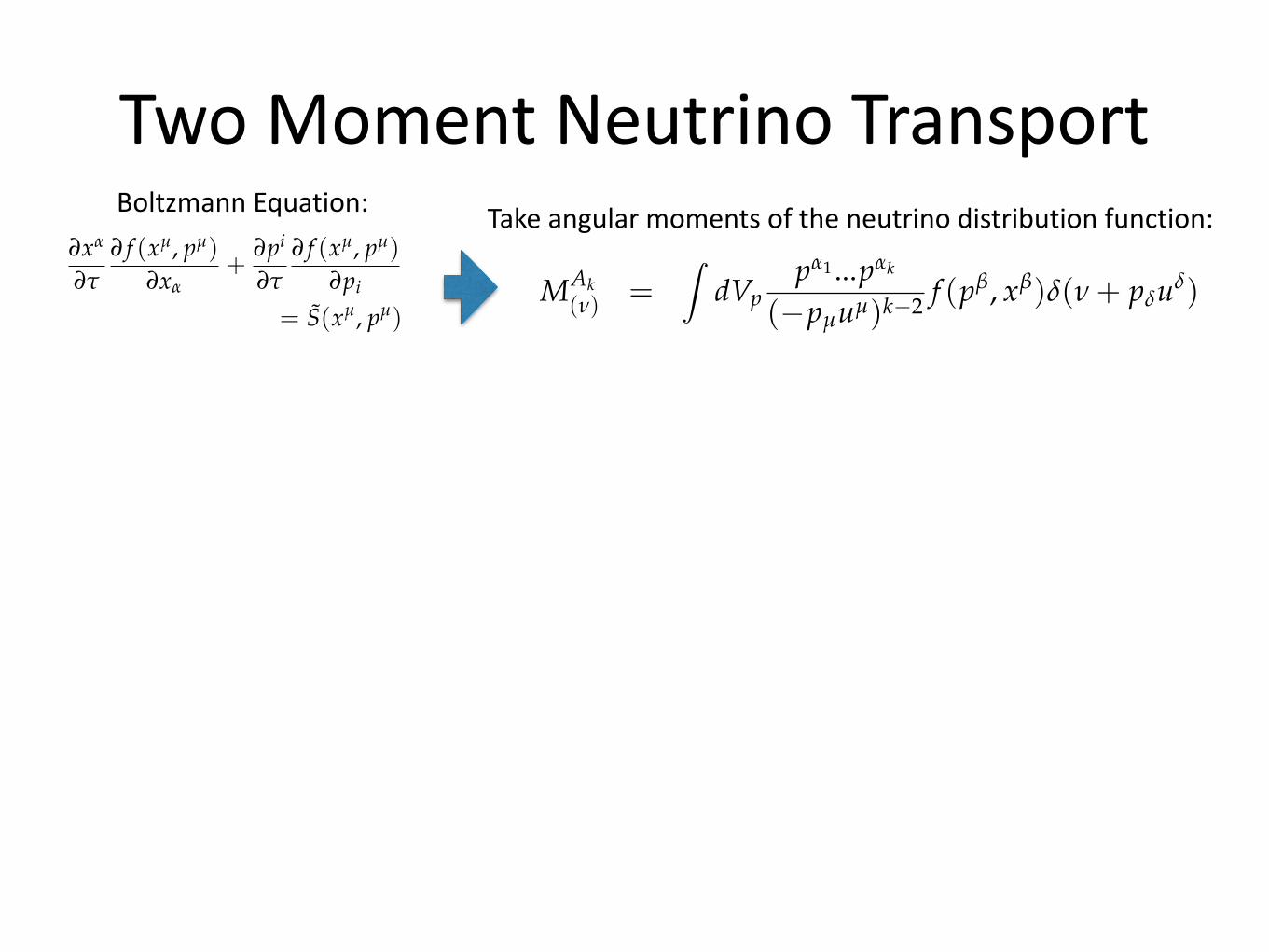
TwoMomentNeutrinoTransportEntropyTakeangularmomentsoftheneutrinodistributionfunction:
4 Things that are still missing
• Relativistic asymptotic flux
• higher-order implicit explicit flux integration (second order currently implemented)
• energy bin coupling
• integration with multipatch
5 Formulation of Transport Moment Equations
The number and energy moments of the radiation field are defined by [2, 4]
MAk(n) =
ZdVp
pa1 ...pak
(�pµ
uµ)k�2 f (pb, xb)d(n + pd
ud)
=Z
dWIn
(xb, W)(la1 + ua1)...(lak + uak).
=Z
dn
0dW0 In
0(xb, W0)(l0a1 + na1)...(l0ak + nak)
⇥d [n� Gn
0(1� l0a
va)]Gk�2(1� l0
a
va)k�2
NAk(n) =
ZdVp
pa1 ...pak
(�pµ
uµ)k�1 f (pb, xb)d(n + pd
ud) =MAk
(n)
n
Here, la
is a unit vector orthogonal to the fluid four velocity pointing in direction W. Theprimed frame is a coordinate observer frame and the last line shows the complicated mixingbetween the moments defined in the fluid rest frame and the laboratory frame. These mo-ments are defined relative to a particular congruence and it is generally hard to map thembetween congruences, none the less they are covariant quantities. Taking the divergence ofthese moments and employing the Lindquist equation gives evolution equations for thesemoments
MAk b
(n) ;b =Z
dVppa1 ...pak pb
(�pl
ul)k�1
(Nd
0(pµ
uµ + n)pgug;b
+k � 1�p
l
ul
pgug;bNd(p
µ
uµ + n) + d(pµ
uµ + n)N;b
)
=∂
∂n
⇣nMAk bg
(n) ub;g
⌘+ (k � 1)MAk bg
(n) ub;g + SAk
(n). (1)
All derivatives in this are taken with fixed p (specifically the derivative of N). The sourceterm is then defined as
SAk(n) =
ZdVpd(n + p
µ
uµ)pa1 ...pak
(�pµ
uµ)k�2
✓∂ f∂l
◆
coll. (2)
3
4 Things that are still missing
• Relativistic asymptotic flux
• higher-order implicit explicit flux integration (second order currently implemented)
• energy bin coupling
• integration with multipatch
5 Formulation of Transport Moment Equations
The number and energy moments of the radiation field are defined by [? ? ]
MAk(n) =
ZdVp
pa1 ...pak
(�pµ
uµ)k�2 f (pb, xb)d(n + pd
ud)
=Z
dWIn
(xb, W)(la1 + ua1)...(lak + uak).
=Z
dn
0dW0 In
0(xb, W0)(l0a1 + na1)...(l0ak + nak)
⇥d [n � Gn
0(1 � l0a
va)]Gk�2(1 � l0
a
va)k�2
NAk(n) =
ZdVp
pa1 ...pak
(�pµ
uµ)k�1 f (pb, xb)d(n + pd
ud) =MAk
(n)
n
Here, la
is a unit vector orthogonal to the fluid four velocity pointing in direction W. Theprimed frame is a coordinate observer frame and the last line shows the complicated mixingbetween the moments defined in the fluid rest frame and the laboratory frame. These mo-ments are defined relative to a particular congruence and it is generally hard to map thembetween congruences, none the less they are covariant quantities. Taking the divergence ofthese moments and employing the Lindquist equation gives evolution equations for thesemoments
Mab
(n) ;b (1)
∂xa
∂t
∂ f (xµ, pµ)∂x
a
+∂pi
∂t
∂ f (xµ, pµ)∂pi
= S(xµ, pµ) (2)
MAk b
(n) ;b =Z
dVppa1 ...pak pb
(�pl
ul)k�1
(Nd
0(pµ
uµ + n)pgug;b
+k � 1�p
l
ul
pgug;bNd(p
µ
uµ + n) + d(pµ
uµ + n)N;b
)
=∂
∂n
⇣nMAk bg
(n) ub;g
⌘+ (k � 1)MAk bg
(n) ub;g + SAk
(n). (3)
3
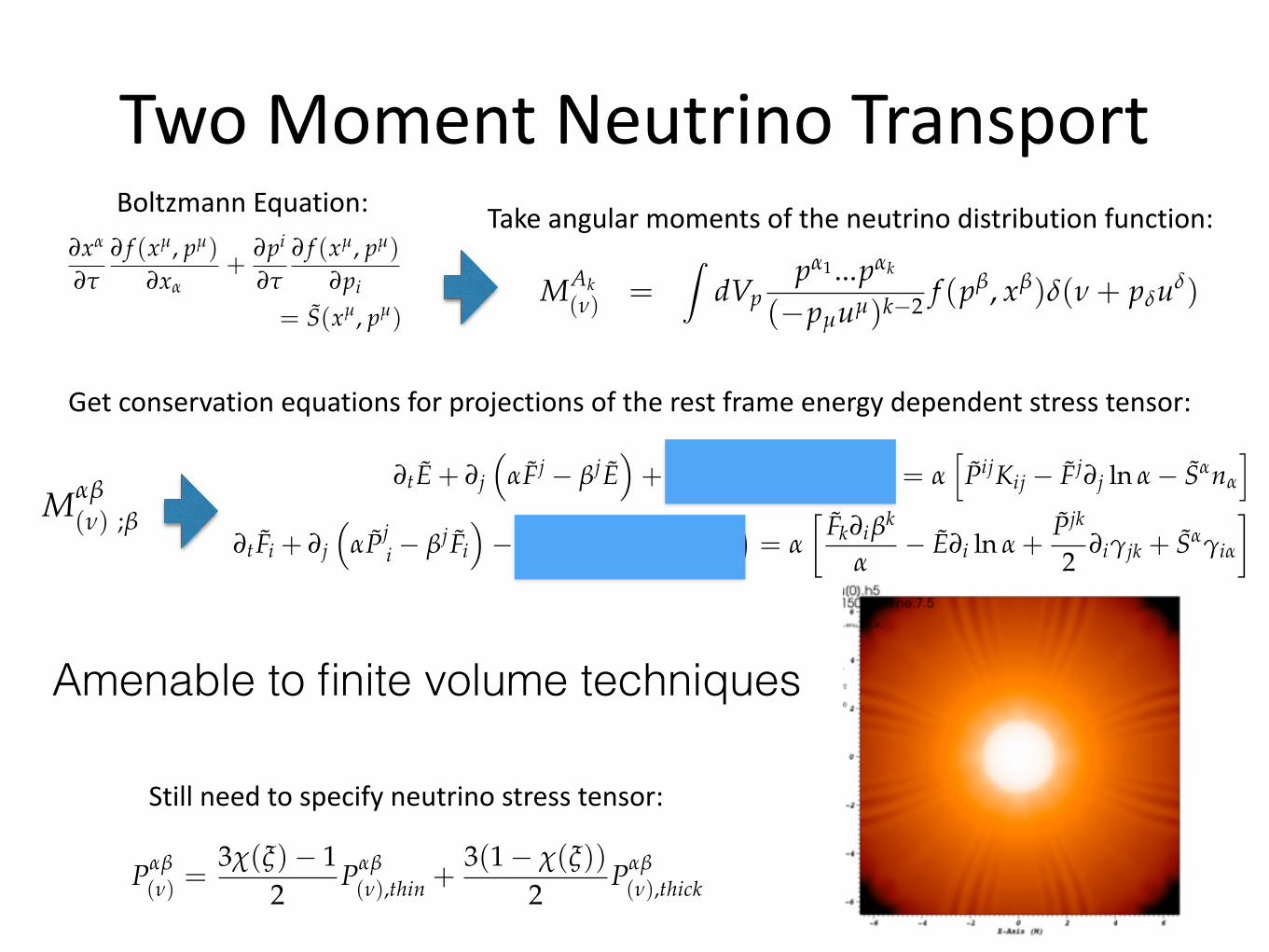
BoltzmannEquation:

TwoMomentNeutrinoTransportEntropyTakeangularmomentsoftheneutrinodistributionfunction:
(I did not carefully check the gravitational source terms in these, they are taken directly from[2]. They can be probably be found from Mabn
a;b and Mab
gia;b, respectively.)
The evolution of the number density can be found in a similar fashion. For coupling to Yeevolution, it is natural to consider the zeroth order moment equation for the number density.We define the 3+1 projection of this moment as
Na = naN +F a = ua
Jn
+Ha
n
. (9)
The number conservation equation is then
∂t (p
gN ) + ∂i
hpg
⇣aF i � b
iN⌘i� ∂
n
ha
pgnNabu
a;b
i= a
pgC(n). (10)
The number flux can be determined from the neutrino stress energy tensor,
F i = g
ia
Na =Gvi
n
J +g
ia
Ha
n
. (11)
We can write the evolution equations in densitized, conservative form by defining MAn =pgMAn . This gives
∂tE + ∂j
⇣aFj � b
j E⌘
+ ∂
n
⇣nan
a
Mabgug;b
⌘= a
hPijKij � Fj
∂j ln a� Sana
i(12)
∂t Fi + ∂j
⇣aPj
i � b
j Fi
⌘� ∂
n
⇣nagia Mabgu
g;b
⌘= a
Fk∂ib
k
a
� E∂i ln a +Pjk
2∂igjk + Sa
gia
�(13)
∂tN + ∂i
⇣aF i � b
iN⌘� ∂
n
hanNabu
a;b
i= aC(n). (14)
6 Redshifting Terms
The third moment, which is required for the energy derivative term, can also be decomposedin the fluid rest frame as
Mlµn
(n) = J(n)uluµun + Hl
(n)uµun + Hµ
(n)ulun + Hn
(n)uluµ + Klµ
(n)un + Kln
(n)uµ + Knµ
(n)ul + Llµn
(n) .(15)
(We drop the (n) subscripts from here on for simplicity). A similar decomposition in terms ofE, Fµ, and Pµn is significantly more complicated because the identities of Thorne ’80 (equa-tions 4.1) are only true for contractions with the velocity field of the fiducial congruence.Luckily, such a decomposition is unnecessary if J, Hµ, Kµn, and Nlµn can be expressed interms of E and Fµ. How Pµn Kµn and Nlµn are specified in terms of E and g
iµ
Fµ defines theclosure.
Expanding the divergence of the four-velocity field of the fluid in terms of its accelerationaa, expansion Q, shear s
ab, and its rotation w
ab, we find
Mabgua;b = ug
Q3
J + Haaa
+ Kab
s
ab
�+
Q3
Hg + aa
Kag + s
ab
Labg. (16)
5
4 Things that are still missing
• Relativistic asymptotic flux
• higher-order implicit explicit flux integration (second order currently implemented)
• energy bin coupling
• integration with multipatch
5 Formulation of Transport Moment Equations
The number and energy moments of the radiation field are defined by [2, 4]
MAk(n) =
ZdVp
pa1 ...pak
(�pµ
uµ)k�2 f (pb, xb)d(n + pd
ud)
=Z
dWIn
(xb, W)(la1 + ua1)...(lak + uak).
=Z
dn
0dW0 In
0(xb, W0)(l0a1 + na1)...(l0ak + nak)
⇥d [n� Gn
0(1� l0a
va)]Gk�2(1� l0
a
va)k�2
NAk(n) =
ZdVp
pa1 ...pak
(�pµ
uµ)k�1 f (pb, xb)d(n + pd
ud) =MAk
(n)
n
Here, la
is a unit vector orthogonal to the fluid four velocity pointing in direction W. Theprimed frame is a coordinate observer frame and the last line shows the complicated mixingbetween the moments defined in the fluid rest frame and the laboratory frame. These mo-ments are defined relative to a particular congruence and it is generally hard to map thembetween congruences, none the less they are covariant quantities. Taking the divergence ofthese moments and employing the Lindquist equation gives evolution equations for thesemoments
MAk b
(n) ;b =Z
dVppa1 ...pak pb
(�pl
ul)k�1
(Nd
0(pµ
uµ + n)pgug;b
+k � 1�p
l
ul
pgug;bNd(p
µ
uµ + n) + d(pµ
uµ + n)N;b
)
=∂
∂n
⇣nMAk bg
(n) ub;g
⌘+ (k � 1)MAk bg
(n) ub;g + SAk
(n). (1)
All derivatives in this are taken with fixed p (specifically the derivative of N). The sourceterm is then defined as
SAk(n) =
ZdVpd(n + p
µ
uµ)pa1 ...pak
(�pµ
uµ)k�2
✓∂ f∂l
◆
coll. (2)
3
Getconservationequationsforprojectionsoftherestframeenergydependentstresstensor:
4 Things that are still missing
• Relativistic asymptotic flux
• higher-order implicit explicit flux integration (second order currently implemented)
• energy bin coupling
• integration with multipatch
5 Formulation of Transport Moment Equations
The number and energy moments of the radiation field are defined by [2, 4]
MAk(n) =
ZdVp
pa1 ...pak
(�pµ
uµ)k�2 f (pb, xb)d(n + pd
ud)
=Z
dWIn
(xb, W)(la1 + ua1)...(lak + uak).
=Z
dn
0dW0 In
0(xb, W0)(l0a1 + na1)...(l0ak + nak)
⇥d [n � Gn
0(1 � l0a
va)]Gk�2(1 � l0
a
va)k�2
NAk(n) =
ZdVp
pa1 ...pak
(�pµ
uµ)k�1 f (pb, xb)d(n + pd
ud) =MAk
(n)
n
Here, la
is a unit vector orthogonal to the fluid four velocity pointing in direction W. Theprimed frame is a coordinate observer frame and the last line shows the complicated mixingbetween the moments defined in the fluid rest frame and the laboratory frame. These mo-ments are defined relative to a particular congruence and it is generally hard to map thembetween congruences, none the less they are covariant quantities. Taking the divergence ofthese moments and employing the Lindquist equation gives evolution equations for thesemoments
Mab
(n) ;b (1)
MAk b
(n) ;b =Z
dVppa1 ...pak pb
(�pl
ul)k�1
(Nd
0(pµ
uµ + n)pgug;b
+k � 1�p
l
ul
pgug;bNd(p
µ
uµ + n) + d(pµ
uµ + n)N;b
)
=∂
∂n
⇣nMAk bg
(n) ub;g
⌘+ (k � 1)MAk bg
(n) ub;g + SAk
(n). (2)
All derivatives in this are taken with fixed p (specifically the derivative of N). The sourceterm is then defined as
SAk(n) =
ZdVpd(n + p
µ
uµ)pa1 ...pak
(�pµ
uµ)k�2
✓∂ f∂l
◆
coll. (3)
3
4 Things that are still missing
• Relativistic asymptotic flux
• higher-order implicit explicit flux integration (second order currently implemented)
• energy bin coupling
• integration with multipatch
5 Formulation of Transport Moment Equations
The number and energy moments of the radiation field are defined by [? ? ]
MAk(n) =
ZdVp
pa1 ...pak
(�pµ
uµ)k�2 f (pb, xb)d(n + pd
ud)
=Z
dWIn
(xb, W)(la1 + ua1)...(lak + uak).
=Z
dn
0dW0 In
0(xb, W0)(l0a1 + na1)...(l0ak + nak)
⇥d [n � Gn
0(1 � l0a
va)]Gk�2(1 � l0
a
va)k�2
NAk(n) =
ZdVp
pa1 ...pak
(�pµ
uµ)k�1 f (pb, xb)d(n + pd
ud) =MAk
(n)
n
Here, la
is a unit vector orthogonal to the fluid four velocity pointing in direction W. Theprimed frame is a coordinate observer frame and the last line shows the complicated mixingbetween the moments defined in the fluid rest frame and the laboratory frame. These mo-ments are defined relative to a particular congruence and it is generally hard to map thembetween congruences, none the less they are covariant quantities. Taking the divergence ofthese moments and employing the Lindquist equation gives evolution equations for thesemoments
Mab
(n) ;b (1)
∂xa
∂t
∂ f (xµ, pµ)∂x
a
+∂pi
∂t
∂ f (xµ, pµ)∂pi
= S(xµ, pµ) (2)
MAk b
(n) ;b =Z
dVppa1 ...pak pb
(�pl
ul)k�1
(Nd
0(pµ
uµ + n)pgug;b
+k � 1�p
l
ul
pgug;bNd(p
µ
uµ + n) + d(pµ
uµ + n)N;b
)
=∂
∂n
⇣nMAk bg
(n) ub;g
⌘+ (k � 1)MAk bg
(n) ub;g + SAk
(n). (3)
3
BoltzmannEquation:
TwoMomentNeutrinoTransportEntropyTakeangularmomentsoftheneutrinodistributionfunction:
(I did not carefully check the gravitational source terms in these, they are taken directly from[2]. They can be probably be found from Mabn
a;b and Mab
gia;b, respectively.)
The evolution of the number density can be found in a similar fashion. For coupling to Yeevolution, it is natural to consider the zeroth order moment equation for the number density.We define the 3+1 projection of this moment as
Na = naN +F a = ua
Jn
+Ha
n
. (9)
The number conservation equation is then
∂t (p
gN ) + ∂i
hpg
⇣aF i � b
iN⌘i� ∂
n
ha
pgnNabu
a;b
i= a
pgC(n). (10)
The number flux can be determined from the neutrino stress energy tensor,
F i = g
ia
Na =Gvi
n
J +g
ia
Ha
n
. (11)
We can write the evolution equations in densitized, conservative form by defining MAn =pgMAn . This gives
∂tE + ∂j
⇣aFj � b
j E⌘
+ ∂
n
⇣nan
a
Mabgug;b
⌘= a
hPijKij � Fj
∂j ln a� Sana
i(12)
∂t Fi + ∂j
⇣aPj
i � b
j Fi
⌘� ∂
n
⇣nagia Mabgu
g;b
⌘= a
Fk∂ib
k
a
� E∂i ln a +Pjk
2∂igjk + Sa
gia
�(13)
∂tN + ∂i
⇣aF i � b
iN⌘� ∂
n
hanNabu
a;b
i= aC(n). (14)
6 Redshifting Terms
The third moment, which is required for the energy derivative term, can also be decomposedin the fluid rest frame as
Mlµn
(n) = J(n)uluµun + Hl
(n)uµun + Hµ
(n)ulun + Hn
(n)uluµ + Klµ
(n)un + Kln
(n)uµ + Knµ
(n)ul + Llµn
(n) .(15)
(We drop the (n) subscripts from here on for simplicity). A similar decomposition in terms ofE, Fµ, and Pµn is significantly more complicated because the identities of Thorne ’80 (equa-tions 4.1) are only true for contractions with the velocity field of the fiducial congruence.Luckily, such a decomposition is unnecessary if J, Hµ, Kµn, and Nlµn can be expressed interms of E and Fµ. How Pµn Kµn and Nlµn are specified in terms of E and g
iµ
Fµ defines theclosure.
Expanding the divergence of the four-velocity field of the fluid in terms of its accelerationaa, expansion Q, shear s
ab, and its rotation w
ab, we find
Mabgua;b = ug
Q3
J + Haaa
+ Kab
s
ab
�+
Q3
Hg + aa
Kag + s
ab
Labg. (16)
5
4 Things that are still missing
• Relativistic asymptotic flux
• higher-order implicit explicit flux integration (second order currently implemented)
• energy bin coupling
• integration with multipatch
5 Formulation of Transport Moment Equations
The number and energy moments of the radiation field are defined by [2, 4]
MAk(n) =
ZdVp
pa1 ...pak
(�pµ
uµ)k�2 f (pb, xb)d(n + pd
ud)
=Z
dWIn
(xb, W)(la1 + ua1)...(lak + uak).
=Z
dn
0dW0 In
0(xb, W0)(l0a1 + na1)...(l0ak + nak)
⇥d [n� Gn
0(1� l0a
va)]Gk�2(1� l0
a
va)k�2
NAk(n) =
ZdVp
pa1 ...pak
(�pµ
uµ)k�1 f (pb, xb)d(n + pd
ud) =MAk
(n)
n
Here, la
is a unit vector orthogonal to the fluid four velocity pointing in direction W. Theprimed frame is a coordinate observer frame and the last line shows the complicated mixingbetween the moments defined in the fluid rest frame and the laboratory frame. These mo-ments are defined relative to a particular congruence and it is generally hard to map thembetween congruences, none the less they are covariant quantities. Taking the divergence ofthese moments and employing the Lindquist equation gives evolution equations for thesemoments
MAk b
(n) ;b =Z
dVppa1 ...pak pb
(�pl
ul)k�1
(Nd
0(pµ
uµ + n)pgug;b
+k � 1�p
l
ul
pgug;bNd(p
µ
uµ + n) + d(pµ
uµ + n)N;b
)
=∂
∂n
⇣nMAk bg
(n) ub;g
⌘+ (k � 1)MAk bg
(n) ub;g + SAk
(n). (1)
All derivatives in this are taken with fixed p (specifically the derivative of N). The sourceterm is then defined as
SAk(n) =
ZdVpd(n + p
µ
uµ)pa1 ...pak
(�pµ
uµ)k�2
✓∂ f∂l
◆
coll. (2)
3
and
Aa
thick = ha
µ
un
Pµn
(n),thick = Gvb
Pab
(n),thick + G(na + va)Bthick
= an,thickna + av,thickva + aF,thickFa (62)
with coefficients
an,thick = GBthick
av,thick = GBthick +G
2G2 + 1⇥(3� 2G2)E +
�2G2 � 1
�(v · F)
⇤
aF,thick = G(v · v). (63)
For implementation, the quantities Jthick, Hithick, and Pij
thick need to be calculated at all inter-faces between zones (spatial and energy interfaces). The quantities Kµn
thick, and Nabd
thick are alsorequired for calculating the fluxes in energy space and must be constructed at the cell edges.Symmetries of these tensors need to be exploited to minimize the number of floating pointoperations required to construct them.
7.1 Lab Frame Formulation
This is what is currently implemented, it follows [2] directly.
The radiation stress tensor is specified by
Pab
(n) =3c(x)� 1
2Pab
(n),thin +3(1� c(x))
2Pab
(n),thick. (64)
wherex
2 =H
a
Ha
J2 . (65)
This represents an implicit equation for x which must be solved iteratively. The rest frameneutrino energy is
J = uluw Mlw
= B0 + dthinBthin + dthickBthick (66)
whereB0 = G2E� 2G2(v · F). (67)
The rest frame flux is
Ha
= �hl
a
uw Mlw
= �(an,0 + dthinan,thin + dthickan,thick)na
�(av,0 + dthinav,thin + dthickav,thick)va
�(aF,0 + dthickaF,thick)Fa
�dthina f ,thin fa
(68)
where
an,0 = G(G2 � 1)E� G3(v · F) + G(1� G2)(v · F)= GB0 + G (v · F� E) (69)
av,0 = G3E� 2G3(v · F) = GB0 (70)aF,0 = �G. (71)
10
Getconservationequationsforprojectionsoftherestframeenergydependentstresstensor:
Stillneedtospecifyneutrinostresstensor:
Amenable to finite volume techniques
4 Things that are still missing
• Relativistic asymptotic flux
• higher-order implicit explicit flux integration (second order currently implemented)
• energy bin coupling
• integration with multipatch
5 Formulation of Transport Moment Equations
The number and energy moments of the radiation field are defined by [2, 4]
MAk(n) =
ZdVp
pa1 ...pak
(�pµ
uµ)k�2 f (pb, xb)d(n + pd
ud)
=Z
dWIn
(xb, W)(la1 + ua1)...(lak + uak).
=Z
dn
0dW0 In
0(xb, W0)(l0a1 + na1)...(l0ak + nak)
⇥d [n � Gn
0(1 � l0a
va)]Gk�2(1 � l0
a
va)k�2
NAk(n) =
ZdVp
pa1 ...pak
(�pµ
uµ)k�1 f (pb, xb)d(n + pd
ud) =MAk
(n)
n
Here, la
is a unit vector orthogonal to the fluid four velocity pointing in direction W. Theprimed frame is a coordinate observer frame and the last line shows the complicated mixingbetween the moments defined in the fluid rest frame and the laboratory frame. These mo-ments are defined relative to a particular congruence and it is generally hard to map thembetween congruences, none the less they are covariant quantities. Taking the divergence ofthese moments and employing the Lindquist equation gives evolution equations for thesemoments
Mab
(n) ;b (1)
MAk b
(n) ;b =Z
dVppa1 ...pak pb
(�pl
ul)k�1
(Nd
0(pµ
uµ + n)pgug;b
+k � 1�p
l
ul
pgug;bNd(p
µ
uµ + n) + d(pµ
uµ + n)N;b
)
=∂
∂n
⇣nMAk bg
(n) ub;g
⌘+ (k � 1)MAk bg
(n) ub;g + SAk
(n). (2)
All derivatives in this are taken with fixed p (specifically the derivative of N). The sourceterm is then defined as
SAk(n) =
ZdVpd(n + p
µ
uµ)pa1 ...pak
(�pµ
uµ)k�2
✓∂ f∂l
◆
coll. (3)
3
4 Things that are still missing
• Relativistic asymptotic flux
• higher-order implicit explicit flux integration (second order currently implemented)
• energy bin coupling
• integration with multipatch
5 Formulation of Transport Moment Equations
The number and energy moments of the radiation field are defined by [? ? ]
MAk(n) =
ZdVp
pa1 ...pak
(�pµ
uµ)k�2 f (pb, xb)d(n + pd
ud)
=Z
dWIn
(xb, W)(la1 + ua1)...(lak + uak).
=Z
dn
0dW0 In
0(xb, W0)(l0a1 + na1)...(l0ak + nak)
⇥d [n � Gn
0(1 � l0a
va)]Gk�2(1 � l0
a
va)k�2
NAk(n) =
ZdVp
pa1 ...pak
(�pµ
uµ)k�1 f (pb, xb)d(n + pd
ud) =MAk
(n)
n
Here, la
is a unit vector orthogonal to the fluid four velocity pointing in direction W. Theprimed frame is a coordinate observer frame and the last line shows the complicated mixingbetween the moments defined in the fluid rest frame and the laboratory frame. These mo-ments are defined relative to a particular congruence and it is generally hard to map thembetween congruences, none the less they are covariant quantities. Taking the divergence ofthese moments and employing the Lindquist equation gives evolution equations for thesemoments
Mab
(n) ;b (1)
∂xa
∂t
∂ f (xµ, pµ)∂x
a
+∂pi
∂t
∂ f (xµ, pµ)∂pi
= S(xµ, pµ) (2)
MAk b
(n) ;b =Z
dVppa1 ...pak pb
(�pl
ul)k�1
(Nd
0(pµ
uµ + n)pgug;b
+k � 1�p
l
ul
pgug;bNd(p
µ
uµ + n) + d(pµ
uµ + n)N;b
)
=∂
∂n
⇣nMAk bg
(n) ub;g
⌘+ (k � 1)MAk bg
(n) ub;g + SAk
(n). (3)
3
BoltzmannEquation:
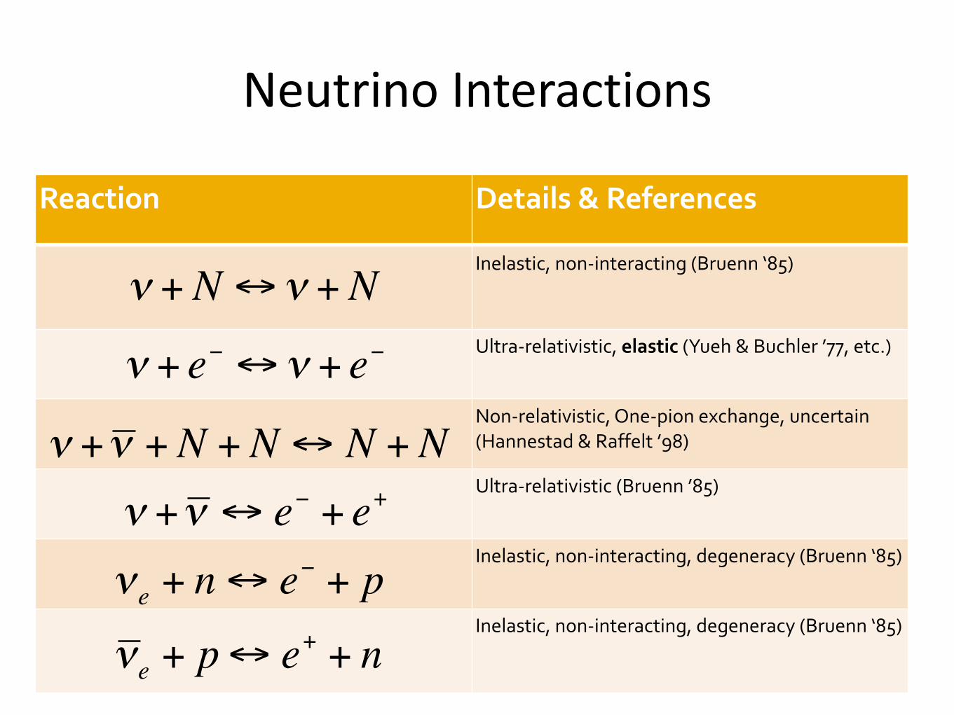
Reaction Details&References
Inelastic,non-interacting(Bruenn‘85)
Ultra-relativistic,elastic(Yueh&Buchler’77,etc.)
Non-relativistic,One-pionexchange,uncertain(Hannestad&Raffelt’98)
Ultra-relativistic(Bruenn’85)
Inelastic,non-interacting,degeneracy(Bruenn‘85)
Inelastic,non-interacting,degeneracy(Bruenn‘85)
€
ν + N↔ν + N
€
ν + e− ↔ν + e−
€
ν +ν + N + N↔ N + N
€
ν +ν ↔ e− + e+
€
νe + n↔ e− + p
€
ν e + p↔ e+ + n
NeutrinoInteractions
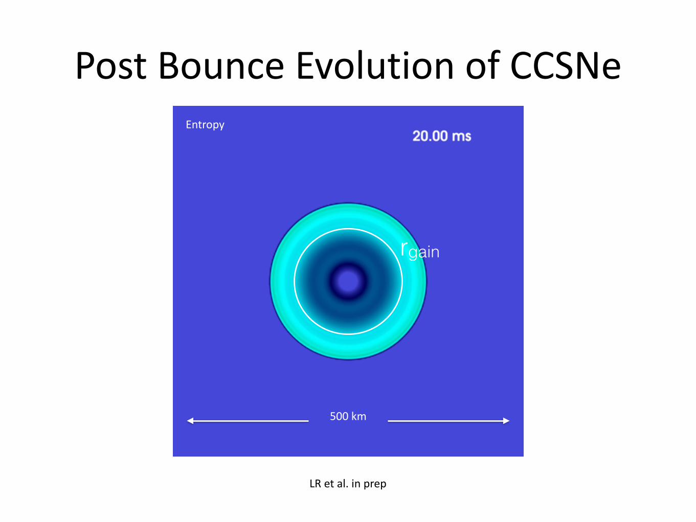
PostBounceEvolutionofCCSNe
LRetal.inprep
500km
Entropy
rgain

NeutrinoHeatingRate
500km
10351033 Erg/cm3/s

Conclusions• M1providesareasonablygoodmethodforradiativetransferinquasi-sphericalsituations
• Longtermevolutionofpost-bounceCCSNeevolutionwithoutanyimposedsymmetries
• Shockrunawayoccursinmanymodels,buthavenotquantifiedpredictedexplosionenergies
• Significantdependenceonresolutionandassumedsymmetries
• Moredetailedanalysisofpost-shockflowrequired